All posts by Vikas Omer

Get started with data integration from Amazon S3 to Amazon Redshift using AWS Glue interactive sessions

Post Syndicated from Vikas Omer original https://aws.amazon.com/blogs/big-data/get-started-with-data-integration-from-amazon-s3-to-amazon-redshift-using-aws-glue-interactive-sessions/

Organizations are placing a high priority on data integration, especially to support analytics, machine learning (ML), business intelligence (BI), and application development initiatives. Data is growing exponentially and is generated by increasingly diverse data sources. Data integration becomes challenging when processing data at scale and the inherent heavy lifting associated with infrastructure required to manage it. This is one of the key reasons why organizations are constantly looking for easy-to-use and low maintenance data integration solutions to move data from one location to another or to consolidate their business data from several sources into a centralized location to make strategic business decisions.

Most organizations use Spark for their big data processing needs. If you’re looking to simplify data integration, and don’t want the hassle of spinning up servers, managing resources, or setting up Spark clusters, we have the solution for you.

AWS Glue is a serverless data integration service that makes it easy to discover, prepare, and combine data for analytics, ML, and application development. AWS Glue provides both visual and code-based interfaces to make data integration simple and accessible for everyone.

If you prefer a code-based experience and want to interactively author data integration jobs, we recommend interactive sessions. Interactive sessions is a recently launched AWS Glue feature that allows you to interactively develop AWS Glue processes, run and test each step, and view the results.

There are different options to use interactive sessions. You can create and work with interactive sessions through the AWS Command Line Interface (AWS CLI) and API. You can also use Jupyter-compatible notebooks to visually author and test your notebook scripts. Interactive sessions provide a Jupyter kernel that integrates almost anywhere that Jupyter does, including integrating with IDEs such as PyCharm, IntelliJ, and Visual Studio Code. This enables you to author code in your local environment and run it seamlessly on the interactive session backend. You can also start a notebook through AWS Glue Studio; all the configuration steps are done for you so that you can explore your data and start developing your job script after only a few seconds. When the code is ready, you can configure, schedule, and monitor job notebooks as AWS Glue jobs.

If you haven’t tried AWS Glue interactive sessions before, this post is highly recommended. We work through a simple scenario where you might need to incrementally load data from Amazon Simple Storage Service (Amazon S3) into Amazon Redshift or transform and enrich your data before loading into Amazon Redshift. In this post, we use interactive sessions within an AWS Glue Studio notebook to load the NYC Taxi dataset into an Amazon Redshift Serverless cluster, query the loaded dataset, save our Jupyter notebook as a job, and schedule it to run using a cron expression. Let’s get started.

Solution overview

We walk you through the following steps:

  1. Set up an AWS Glue Jupyter notebook with interactive sessions.
  2. Use notebook’s magics, including AWS Glue connection and bookmarks.
  3. Read data from Amazon S3, and transform and load it into Redshift Serverless.
  4. Save the notebook as an AWS Glue job and schedule it to run.

Prerequisites

For this walkthrough, we must complete the following prerequisites:

  1. Upload Yellow Taxi Trip Records data and the taxi zone lookup table datasets into Amazon S3. Steps to do that are listed in the next section.
  2. Prepare the necessary AWS Identity and Access Management (IAM) policies and roles to work with AWS Glue Studio Jupyter notebooks, interactive sessions, and AWS Glue.
  3. Create the AWS Glue connection for Redshift Serverless.

Upload datasets into Amazon S3

Download Yellow Taxi Trip Records data and taxi zone lookup table data to your local environment. For this post, we download the January 2022 data for yellow taxi trip records data in Parquet format. The taxi zone lookup data is in CSV format. You can also download the data dictionary for the trip record dataset.

  1. On the Amazon S3 console, create a bucket called my-first-aws-glue-is-project-<random number> in the us-east-1 Region to store the data.S3 bucket names must be unique across all AWS accounts in all the Regions.
  2. Create folders nyc_yellow_taxi and taxi_zone_lookup in the bucket you just created and upload the files you downloaded.
    Your folder structures should look like the following screenshots.s3 yellow taxi datas3 lookup data

Prepare IAM policies and role

Let’s prepare the necessary IAM policies and role to work with AWS Glue Studio Jupyter notebooks and interactive sessions. To get started with notebooks in AWS Glue Studio, refer to Getting started with notebooks in AWS Glue Studio.

Create IAM policies for the AWS Glue notebook role

Create the policy AWSGlueInteractiveSessionPassRolePolicy with the following permissions:

{
    "Version": "2012-10-17",
    "Statement": [
        {
        "Effect": "Allow",
        "Action": "iam:PassRole",
        "Resource":"arn:aws:iam::<AWS account ID>:role/AWSGlueServiceRole-GlueIS"
        }
    ]
}

This policy allows the AWS Glue notebook role to pass to interactive sessions so that the same role can be used in both places. Note that AWSGlueServiceRole-GlueIS is the role that we create for the AWS Glue Studio Jupyter notebook in a later step. Next, create the policy AmazonS3Access-MyFirstGlueISProject with the following permissions:

{
    "Version": "2012-10-17",
    "Statement": [
        {
            "Effect": "Allow",
            "Action": [
                "s3:GetObject",
                "s3:ListBucket"
            ],
            "Resource": [
                "arn:aws:s3:::<your s3 bucket name>",
                "arn:aws:s3:::<your s3 bucket name>/*"
            ]
        }
    ]
}

This policy allows the AWS Glue notebook role to access data in the S3 bucket.

Create an IAM role for the AWS Glue notebook

Create a new AWS Glue role called AWSGlueServiceRole-GlueIS with the following policies attached to it:

Create the AWS Glue connection for Redshift Serverless

Now we’re ready to configure a Redshift Serverless security group to connect with AWS Glue components.

  1. On the Redshift Serverless console, open the workgroup you’re using.
    You can find all the namespaces and workgroups on the Redshift Serverless dashboard.
  2. Under Data access, choose Network and security.
  3. Choose the link for the Redshift Serverless VPC security group.redshift serverless vpc security groupYou’re redirected to the Amazon Elastic Compute Cloud (Amazon EC2) console.
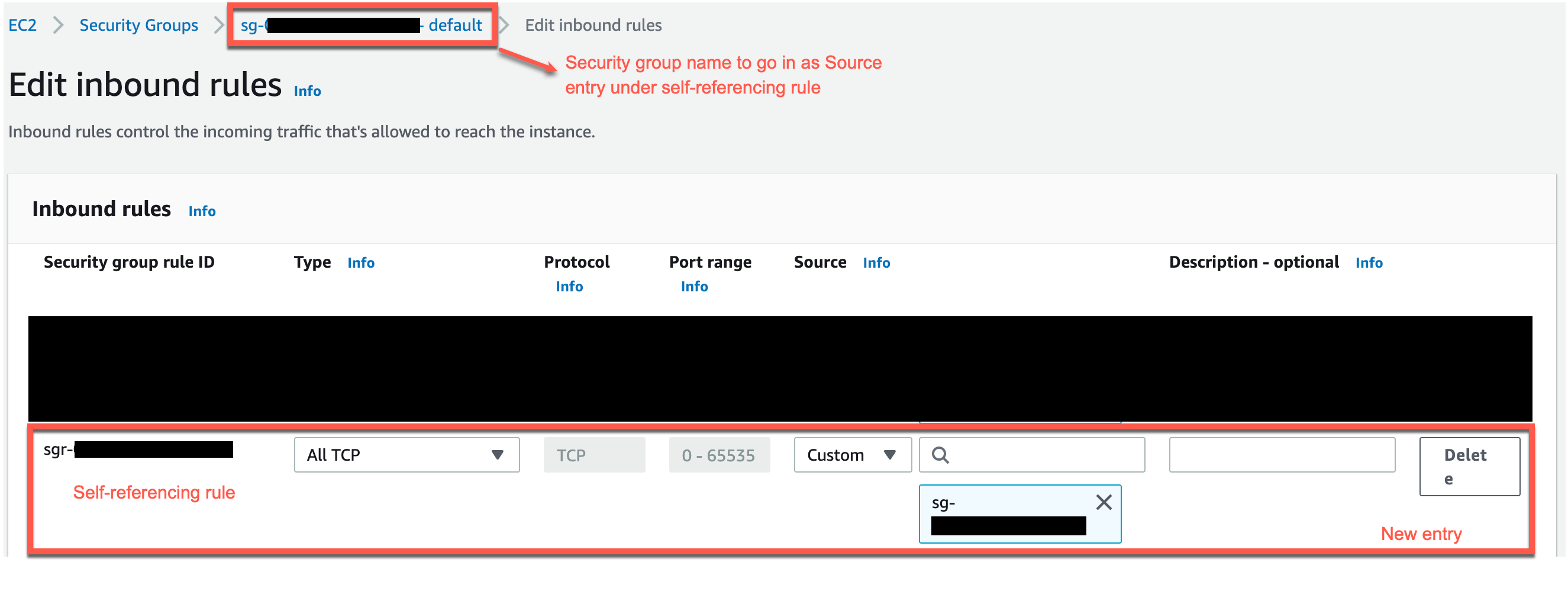
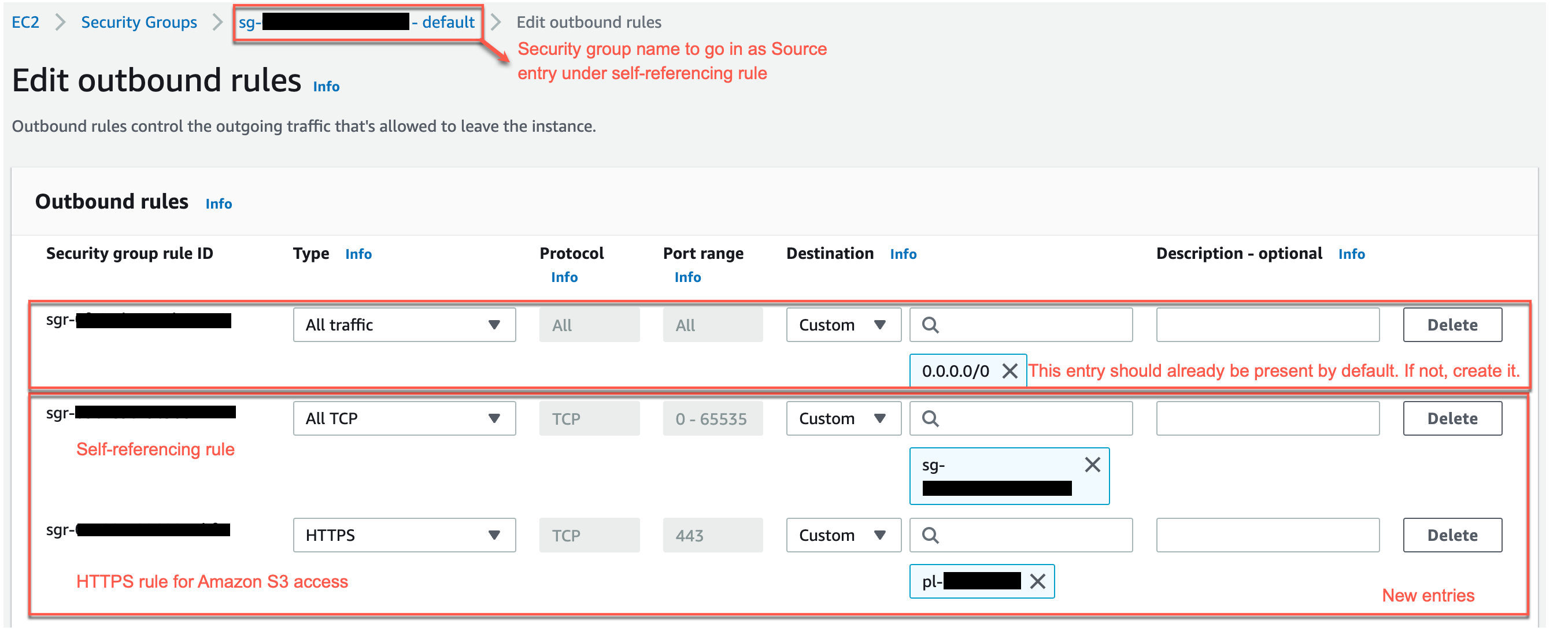
  4. In the Redshift Serverless security group details, under Inbound rules, choose Edit inbound rules.
  5. Add a self-referencing rule to allow AWS Glue components to communicate:
    1. For Type, choose All TCP.
    2. For Protocol, choose TCP.
    3. For Port range, include all ports.
    4. For Source, use the same security group as the group ID.
      redshift inbound security group
  6. Similarly, add the following outbound rules:
    1. A self-referencing rule with Type as All TCP, Protocol as TCP, Port range including all ports, and Destination as the same security group as the group ID.
    2. An HTTPS rule for Amazon S3 access. The s3-prefix-list-id value is required in the security group rule to allow traffic from the VPC to the Amazon S3 VPC endpoint.
      redshift outbound security group

If you don’t have an Amazon S3 VPC endpoint, you can create one on the Amazon Virtual Private Cloud (Amazon VPC) console.

s3 vpc endpoint

You can check the value for s3-prefix-list-id on the Managed prefix lists page on the Amazon VPC console.

s3 prefix list

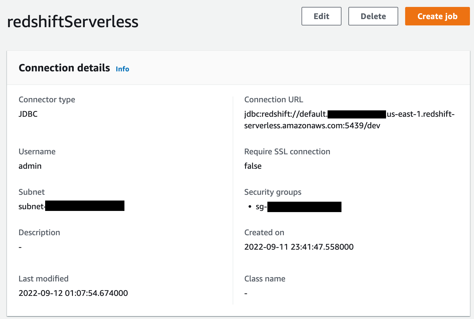
Next, go to the Connectors page on AWS Glue Studio and create a new JDBC connection called redshiftServerless to your Redshift Serverless cluster (unless one already exists). You can find the Redshift Serverless endpoint details under your workgroup’s General Information section. The connection setting looks like the following screenshot.

redshift serverless connection page

Write interactive code on an AWS Glue Studio Jupyter notebook powered by interactive sessions

Now you can get started with writing interactive code using AWS Glue Studio Jupyter notebook powered by interactive sessions. Note that it’s a good practice to keep saving the notebook at regular intervals while you work through it.

  1. On the AWS Glue Studio console, create a new job.
  2. Select Jupyter Notebook and select Create a new notebook from scratch.
  3. Choose Create.
    glue interactive session create notebook
  4. For Job name, enter a name (for example, myFirstGlueISProject).
  5. For IAM Role, choose the role you created (AWSGlueServiceRole-GlueIS).
  6. Choose Start notebook job.
    glue interactive session notebook setupAfter the notebook is initialized, you can see some of the available magics and a cell with boilerplate code. To view all the magics of interactive sessions, run %help in a cell to print a full list. With the exception of %%sql, running a cell of only magics doesn’t start a session, but sets the configuration for the session that starts when you run your first cell of code.glue interactive session jupyter notebook initializationFor this post, we configure AWS Glue with version 3.0, three G.1X workers, idle timeout, and an Amazon Redshift connection with the help of available magics.
  7. Let’s enter the following magics into our first cell and run it:
    %glue_version 3.0
    %number_of_workers 3
    %worker_type G.1X
    %idle_timeout 60
    %connections redshiftServerless

    We get the following response:

    Welcome to the Glue Interactive Sessions Kernel
    For more information on available magic commands, please type %help in any new cell.
    
    Please view our Getting Started page to access the most up-to-date information on the Interactive Sessions kernel: https://docs.aws.amazon.com/glue/latest/dg/interactive-sessions.html
    Installed kernel version: 0.35 
    Setting Glue version to: 3.0
    Previous number of workers: 5
    Setting new number of workers to: 3
    Previous worker type: G.1X
    Setting new worker type to: G.1X
    Current idle_timeout is 2880 minutes.
    idle_timeout has been set to 60 minutes.
    Connections to be included:
    redshiftServerless

  8. Let’s run our first code cell (boilerplate code) to start an interactive notebook session within a few seconds:
    import sys
    from awsglue.transforms import *
    from awsglue.utils import getResolvedOptions
    from pyspark.context import SparkContext
    from awsglue.context import GlueContext
    from awsglue.job import Job
      
    sc = SparkContext.getOrCreate()
    glueContext = GlueContext(sc)
    spark = glueContext.spark_session
    job = Job(glueContext)

    We get the following response:

    Authenticating with environment variables and user-defined glue_role_arn:arn:aws:iam::xxxxxxxxxxxx:role/AWSGlueServiceRole-GlueIS
    Attempting to use existing AssumeRole session credentials.
    Trying to create a Glue session for the kernel.
    Worker Type: G.1X
    Number of Workers: 3
    Session ID: 7c9eadb1-9f9b-424f-9fba-d0abc57e610d
    Applying the following default arguments:
    --glue_kernel_version 0.35
    --enable-glue-datacatalog true
    --job-bookmark-option job-bookmark-enable
    Waiting for session 7c9eadb1-9f9b-424f-9fba-d0abc57e610d to get into ready status...
    Session 7c9eadb1-9f9b-424f-9fba-d0abc57e610d has been created

  9. Next, read the NYC yellow taxi data from the S3 bucket into an AWS Glue dynamic frame:
    nyc_taxi_trip_input_dyf = glueContext.create_dynamic_frame.from_options(
        connection_type = "s3", 
        connection_options = {
            "paths": ["s3://<your-s3-bucket-name>/nyc_yellow_taxi/"]
        }, 
        format = "parquet",
        transformation_ctx = "nyc_taxi_trip_input_dyf"
    )

    Let’s count the number of rows, look at the schema and a few rows of the dataset.

  10. Count the rows with the following code:
    nyc_taxi_trip_input_df = nyc_taxi_trip_input_dyf.toDF()
    nyc_taxi_trip_input_df.count()

    We get the following response:

    2463931

  11. View the schema with the following code:
    nyc_taxi_trip_input_df.printSchema()

    We get the following response:

    root
     |-- VendorID: long (nullable = true)
     |-- tpep_pickup_datetime: timestamp (nullable = true)
     |-- tpep_dropoff_datetime: timestamp (nullable = true)
     |-- passenger_count: double (nullable = true)
     |-- trip_distance: double (nullable = true)
     |-- RatecodeID: double (nullable = true)
     |-- store_and_fwd_flag: string (nullable = true)
     |-- PULocationID: long (nullable = true)
     |-- DOLocationID: long (nullable = true)
     |-- payment_type: long (nullable = true)
     |-- fare_amount: double (nullable = true)
     |-- extra: double (nullable = true)
     |-- mta_tax: double (nullable = true)
     |-- tip_amount: double (nullable = true)
     |-- tolls_amount: double (nullable = true)
     |-- improvement_surcharge: double (nullable = true)
     |-- total_amount: double (nullable = true)
     |-- congestion_surcharge: double (nullable = true)
     |-- airport_fee: double (nullable = true)

  12. View a few rows of the dataset with the following code:
    nyc_taxi_trip_input_df.show(5)

    We get the following response:

    +--------+--------------------+---------------------+---------------+-------------+----------+------------------+------------+------------+------------+-----------+-----+-------+----------+------------+---------------------+------------+--------------------+-----------+
    |VendorID|tpep_pickup_datetime|tpep_dropoff_datetime|passenger_count|trip_distance|RatecodeID|store_and_fwd_flag|PULocationID|DOLocationID|payment_type|fare_amount|extra|mta_tax|tip_amount|tolls_amount|improvement_surcharge|total_amount|congestion_surcharge|airport_fee|
    +--------+--------------------+---------------------+---------------+-------------+----------+------------------+------------+------------+------------+-----------+-----+-------+----------+------------+---------------------+------------+--------------------+-----------+
    |       2| 2022-01-18 15:04:43|  2022-01-18 15:12:51|            1.0|         1.13|       1.0|                 N|         141|         229|           2|        7.0|  0.0|    0.5|       0.0|         0.0|                  0.3|        10.3|                 2.5|        0.0|
    |       2| 2022-01-18 15:03:28|  2022-01-18 15:15:52|            2.0|         1.36|       1.0|                 N|         237|         142|           1|        9.5|  0.0|    0.5|      2.56|         0.0|                  0.3|       15.36|                 2.5|        0.0|
    |       1| 2022-01-06 17:49:22|  2022-01-06 17:57:03|            1.0|          1.1|       1.0|                 N|         161|         229|           2|        7.0|  3.5|    0.5|       0.0|         0.0|                  0.3|        11.3|                 2.5|        0.0|
    |       2| 2022-01-09 20:00:55|  2022-01-09 20:04:14|            1.0|         0.56|       1.0|                 N|         230|         230|           1|        4.5|  0.5|    0.5|      1.66|         0.0|                  0.3|        9.96|                 2.5|        0.0|
    |       2| 2022-01-24 16:16:53|  2022-01-24 16:31:36|            1.0|         2.02|       1.0|                 N|         163|         234|           1|       10.5|  1.0|    0.5|       3.7|         0.0|                  0.3|        18.5|                 2.5|        0.0|
    +--------+--------------------+---------------------+---------------+-------------+----------+------------------+------------+------------+------------+-----------+-----+-------+----------+------------+---------------------+------------+--------------------+-----------+
    only showing top 5 rows

  13. Now, read the taxi zone lookup data from the S3 bucket into an AWS Glue dynamic frame:
    nyc_taxi_zone_lookup_dyf = glueContext.create_dynamic_frame.from_options(
        connection_type = "s3", 
        connection_options = {
            "paths": ["s3://<your-s3-bucket-name>/taxi_zone_lookup/"]
        }, 
        format = "csv",
        format_options= {
            'withHeader': True
        },
        transformation_ctx = "nyc_taxi_zone_lookup_dyf"
    )

    Let’s count the number of rows, look at the schema and a few rows of the dataset.

  14. Count the rows with the following code:
    nyc_taxi_zone_lookup_df = nyc_taxi_zone_lookup_dyf.toDF()
    nyc_taxi_zone_lookup_df.count()

    We get the following response:

    265

  15. View the schema with the following code:
    nyc_taxi_zone_lookup_apply_mapping_dyf.toDF().printSchema()

    We get the following response:

    root
     |-- LocationID: string (nullable = true)
     |-- Borough: string (nullable = true)
     |-- Zone: string (nullable = true)
     |-- service_zone: string (nullable = true)

  16. View a few rows with the following code:
    nyc_taxi_zone_lookup_df.show(5)

    We get the following response:

    +----------+-------------+--------------------+------------+
    |LocationID|      Borough|                Zone|service_zone|
    +----------+-------------+--------------------+------------+
    |         1|          EWR|      Newark Airport|         EWR|
    |         2|       Queens|         Jamaica Bay|   Boro Zone|
    |         3|        Bronx|Allerton/Pelham G...|   Boro Zone|
    |         4|    Manhattan|       Alphabet City| Yellow Zone|
    |         5|Staten Island|       Arden Heights|   Boro Zone|
    +----------+-------------+--------------------+------------+
    only showing top 5 rows

  17. Based on the data dictionary, lets recalibrate the data types of attributes in dynamic frames corresponding to both dynamic frames:
    nyc_taxi_trip_apply_mapping_dyf = ApplyMapping.apply(
        frame = nyc_taxi_trip_input_dyf, 
        mappings = [
            ("VendorID","Long","VendorID","Integer"), 
            ("tpep_pickup_datetime","Timestamp","tpep_pickup_datetime","Timestamp"), 
            ("tpep_dropoff_datetime","Timestamp","tpep_dropoff_datetime","Timestamp"), 
            ("passenger_count","Double","passenger_count","Integer"), 
            ("trip_distance","Double","trip_distance","Double"),
            ("RatecodeID","Double","RatecodeID","Integer"), 
            ("store_and_fwd_flag","String","store_and_fwd_flag","String"), 
            ("PULocationID","Long","PULocationID","Integer"), 
            ("DOLocationID","Long","DOLocationID","Integer"),
            ("payment_type","Long","payment_type","Integer"), 
            ("fare_amount","Double","fare_amount","Double"),
            ("extra","Double","extra","Double"), 
            ("mta_tax","Double","mta_tax","Double"),
            ("tip_amount","Double","tip_amount","Double"), 
            ("tolls_amount","Double","tolls_amount","Double"), 
            ("improvement_surcharge","Double","improvement_surcharge","Double"), 
            ("total_amount","Double","total_amount","Double"), 
            ("congestion_surcharge","Double","congestion_surcharge","Double"), 
            ("airport_fee","Double","airport_fee","Double")
        ],
        transformation_ctx = "nyc_taxi_trip_apply_mapping_dyf"
    )

    nyc_taxi_zone_lookup_apply_mapping_dyf = ApplyMapping.apply(
        frame = nyc_taxi_zone_lookup_dyf, 
        mappings = [ 
            ("LocationID","String","LocationID","Integer"), 
            ("Borough","String","Borough","String"), 
            ("Zone","String","Zone","String"), 
            ("service_zone","String", "service_zone","String")
        ],
        transformation_ctx = "nyc_taxi_zone_lookup_apply_mapping_dyf"
    )

  18. Now let’s check their schema:
    nyc_taxi_trip_apply_mapping_dyf.toDF().printSchema()

    We get the following response:

    root
     |-- VendorID: integer (nullable = true)
     |-- tpep_pickup_datetime: timestamp (nullable = true)
     |-- tpep_dropoff_datetime: timestamp (nullable = true)
     |-- passenger_count: integer (nullable = true)
     |-- trip_distance: double (nullable = true)
     |-- RatecodeID: integer (nullable = true)
     |-- store_and_fwd_flag: string (nullable = true)
     |-- PULocationID: integer (nullable = true)
     |-- DOLocationID: integer (nullable = true)
     |-- payment_type: integer (nullable = true)
     |-- fare_amount: double (nullable = true)
     |-- extra: double (nullable = true)
     |-- mta_tax: double (nullable = true)
     |-- tip_amount: double (nullable = true)
     |-- tolls_amount: double (nullable = true)
     |-- improvement_surcharge: double (nullable = true)
     |-- total_amount: double (nullable = true)
     |-- congestion_surcharge: double (nullable = true)
     |-- airport_fee: double (nullable = true)

    nyc_taxi_zone_lookup_apply_mapping_dyf.toDF().printSchema()

    We get the following response:

    root
     |-- LocationID: integer (nullable = true)
     |-- Borough: string (nullable = true)
     |-- Zone: string (nullable = true)
     |-- service_zone: string (nullable = true)

  19. Let’s add the column trip_duration to calculate the duration of each trip in minutes to the taxi trip dynamic frame:
    # Function to calculate trip duration in minutes
    def trip_duration(start_timestamp,end_timestamp):
        minutes_diff = (end_timestamp - start_timestamp).total_seconds() / 60.0
        return(minutes_diff)

    # Transformation function for each record
    def transformRecord(rec):
        rec["trip_duration"] = trip_duration(rec["tpep_pickup_datetime"], rec["tpep_dropoff_datetime"])
        return rec
    nyc_taxi_trip_final_dyf = Map.apply(
        frame = nyc_taxi_trip_apply_mapping_dyf, 
        f = transformRecord, 
        transformation_ctx = "nyc_taxi_trip_final_dyf"
    )

    Let’s count the number of rows, look at the schema and a few rows of the dataset after applying the above transformation.

  20. Get a record count with the following code:
    nyc_taxi_trip_final_df = nyc_taxi_trip_final_dyf.toDF()
    nyc_taxi_trip_final_df.count()

    We get the following response:

    2463931

  21. View the schema with the following code:
    nyc_taxi_trip_final_df.printSchema()

    We get the following response:

    root
     |-- extra: double (nullable = true)
     |-- tpep_dropoff_datetime: timestamp (nullable = true)
     |-- trip_duration: double (nullable = true)
     |-- trip_distance: double (nullable = true)
     |-- mta_tax: double (nullable = true)
     |-- improvement_surcharge: double (nullable = true)
     |-- DOLocationID: integer (nullable = true)
     |-- congestion_surcharge: double (nullable = true)
     |-- total_amount: double (nullable = true)
     |-- airport_fee: double (nullable = true)
     |-- payment_type: integer (nullable = true)
     |-- fare_amount: double (nullable = true)
     |-- RatecodeID: integer (nullable = true)
     |-- tpep_pickup_datetime: timestamp (nullable = true)
     |-- VendorID: integer (nullable = true)
     |-- PULocationID: integer (nullable = true)
     |-- tip_amount: double (nullable = true)
     |-- tolls_amount: double (nullable = true)
     |-- store_and_fwd_flag: string (nullable = true)
     |-- passenger_count: integer (nullable = true)

  22. View a few rows with the following code:
    nyc_taxi_trip_final_df.show(5)

    We get the following response:

    +-----+---------------------+------------------+-------------+-------+---------------------+------------+--------------------+------------+-----------+------------+-----------+----------+--------------------+--------+------------+----------+------------+------------------+---------------+
    |extra|tpep_dropoff_datetime|     trip_duration|trip_distance|mta_tax|improvement_surcharge|DOLocationID|congestion_surcharge|total_amount|airport_fee|payment_type|fare_amount|RatecodeID|tpep_pickup_datetime|VendorID|PULocationID|tip_amount|tolls_amount|store_and_fwd_flag|passenger_count|
    +-----+---------------------+------------------+-------------+-------+---------------------+------------+--------------------+------------+-----------+------------+-----------+----------+--------------------+--------+------------+----------+------------+------------------+---------------+
    |  0.0|  2022-01-18 15:12:51| 8.133333333333333|         1.13|    0.5|                  0.3|         229|                 2.5|        10.3|        0.0|           2|        7.0|         1| 2022-01-18 15:04:43|       2|         141|       0.0|         0.0|                 N|              1|
    |  0.0|  2022-01-18 15:15:52|              12.4|         1.36|    0.5|                  0.3|         142|                 2.5|       15.36|        0.0|           1|        9.5|         1| 2022-01-18 15:03:28|       2|         237|      2.56|         0.0|                 N|              2|
    |  3.5|  2022-01-06 17:57:03| 7.683333333333334|          1.1|    0.5|                  0.3|         229|                 2.5|        11.3|        0.0|           2|        7.0|         1| 2022-01-06 17:49:22|       1|         161|       0.0|         0.0|                 N|              1|
    |  0.5|  2022-01-09 20:04:14| 3.316666666666667|         0.56|    0.5|                  0.3|         230|                 2.5|        9.96|        0.0|           1|        4.5|         1| 2022-01-09 20:00:55|       2|         230|      1.66|         0.0|                 N|              1|
    |  1.0|  2022-01-24 16:31:36|14.716666666666667|         2.02|    0.5|                  0.3|         234|                 2.5|        18.5|        0.0|           1|       10.5|         1| 2022-01-24 16:16:53|       2|         163|       3.7|         0.0|                 N|              1|
    +-----+---------------------+------------------+-------------+-------+---------------------+------------+--------------------+------------+-----------+------------+-----------+----------+--------------------+--------+------------+----------+------------+------------------+---------------+
    only showing top 5 rows

  23. Next, load both the dynamic frames into our Amazon Redshift Serverless cluster:
    nyc_taxi_trip_sink_dyf = glueContext.write_dynamic_frame.from_jdbc_conf(
        frame = nyc_taxi_trip_final_dyf, 
        catalog_connection = "redshiftServerless", 
        connection_options =  {"dbtable": "public.f_nyc_yellow_taxi_trip","database": "dev"}, 
        redshift_tmp_dir = "s3://aws-glue-assets-<AWS-account-ID>-us-east-1/temporary/", 
        transformation_ctx = "nyc_taxi_trip_sink_dyf"
    )

    nyc_taxi_zone_lookup_sink_dyf = glueContext.write_dynamic_frame.from_jdbc_conf(
        frame = nyc_taxi_zone_lookup_apply_mapping_dyf, 
        catalog_connection = "redshiftServerless", 
        connection_options = {"dbtable": "public.d_nyc_taxi_zone_lookup", "database": "dev"}, 
        redshift_tmp_dir = "s3://aws-glue-assets-<AWS-account-ID>-us-east-1/temporary/", 
        transformation_ctx = "nyc_taxi_zone_lookup_sink_dyf"
    )

    Now let’s validate the data loaded in Amazon Redshift Serverless cluster by running a few queries in Amazon Redshift query editor v2. You can also use your preferred query editor.

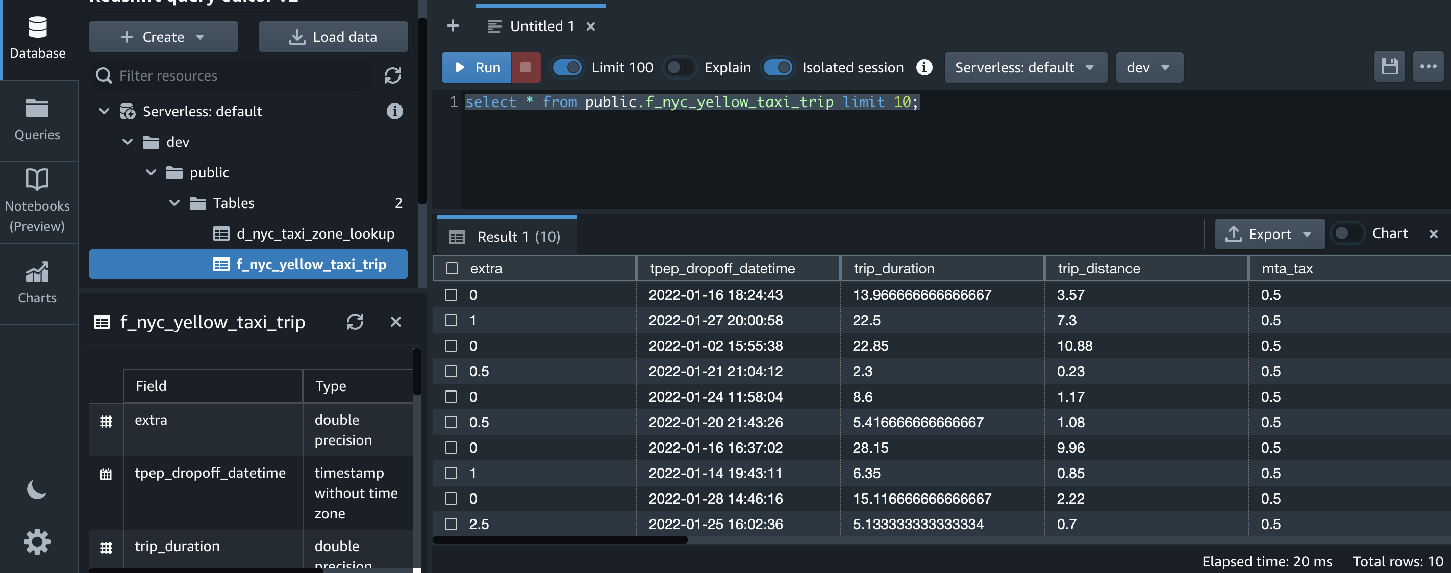
  24. First, we count the number of records and select a few rows in both the target tables (f_nyc_yellow_taxi_trip and d_nyc_taxi_zone_lookup):
    SELECT 'f_nyc_yellow_taxi_trip' AS table_name, COUNT(1) FROM "public"."f_nyc_yellow_taxi_trip"
    UNION ALL
    SELECT 'd_nyc_taxi_zone_lookup' AS table_name, COUNT(1) FROM "public"."d_nyc_taxi_zone_lookup";

    redshift table record count query output

    The number of records in f_nyc_yellow_taxi_trip (2,463,931) and d_nyc_taxi_zone_lookup (265) match the number of records in our input dynamic frame. This validates that all records from files in Amazon S3 have been successfully loaded into Amazon Redshift.

    You can view some of the records for each table with the following commands:

    SELECT * FROM public.f_nyc_yellow_taxi_trip LIMIT 10;

    redshift fact data select query

    SELECT * FROM public.d_nyc_taxi_zone_lookup LIMIT 10;

    redshift lookup data select query

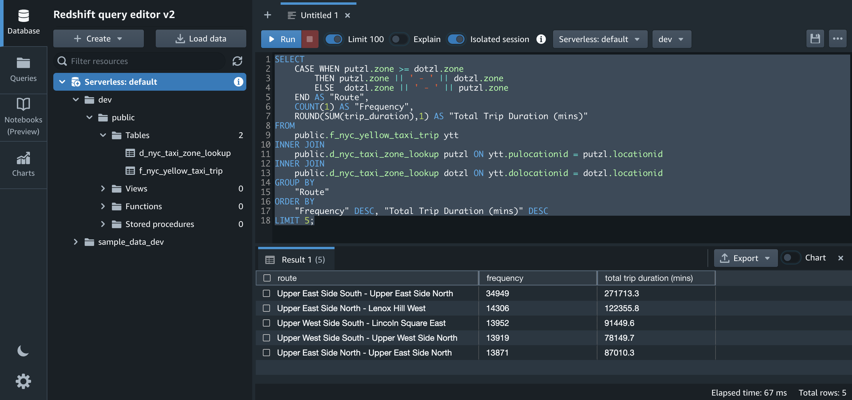
  25. One of the insights that we want to generate from the datasets is to get the top five routes with their trip duration. Let’s run the SQL for that on Amazon Redshift:
    SELECT 
        CASE WHEN putzl.zone >= dotzl.zone 
            THEN putzl.zone || ' - ' || dotzl.zone 
            ELSE  dotzl.zone || ' - ' || putzl.zone 
        END AS "Route",
        COUNT(1) AS "Frequency",
        ROUND(SUM(trip_duration),1) AS "Total Trip Duration (mins)"
    FROM 
        public.f_nyc_yellow_taxi_trip ytt
    INNER JOIN 
        public.d_nyc_taxi_zone_lookup putzl ON ytt.pulocationid = putzl.locationid
    INNER JOIN 
        public.d_nyc_taxi_zone_lookup dotzl ON ytt.dolocationid = dotzl.locationid
    GROUP BY 
        "Route"
    ORDER BY 
        "Frequency" DESC, "Total Trip Duration (mins)" DESC
    LIMIT 5;

    redshift top 5 route query

Transform the notebook into an AWS Glue job and schedule it

Now that we have authored the code and tested its functionality, let’s save it as a job and schedule it.

Let’s first enable job bookmarks. Job bookmarks help AWS Glue maintain state information and prevent the reprocessing of old data. With job bookmarks, you can process new data when rerunning on a scheduled interval.

  1. Add the following magic command after the first cell that contains other magic commands initialized during authoring the code:
    %%configure
    {
        "--job-bookmark-option": "job-bookmark-enable"
    }

    To initialize job bookmarks, we run the following code with the name of the job as the default argument (myFirstGlueISProject for this post). Job bookmarks store the states for a job. You should always have job.init() in the beginning of the script and the job.commit() at the end of the script. These two functions are used to initialize the bookmark service and update the state change to the service. Bookmarks won’t work without calling them.

  2. Add the following piece of code after the boilerplate code:
    params = []
    if '--JOB_NAME' in sys.argv:
        params.append('JOB_NAME')
    args = getResolvedOptions(sys.argv, params)
    if 'JOB_NAME' in args:
        jobname = args['JOB_NAME']
    else:
        jobname = "myFirstGlueISProject"
    job.init(jobname, args)

  3. Then comment out all the lines of code that were authored to verify the desired outcome and aren’t necessary for the job to deliver its purpose:
    #nyc_taxi_trip_input_df = nyc_taxi_trip_input_dyf.toDF()
    #nyc_taxi_trip_input_df.count()
    #nyc_taxi_trip_input_df.printSchema()
    #nyc_taxi_trip_input_df.show(5)
    
    #nyc_taxi_zone_lookup_df = nyc_taxi_zone_lookup_dyf.toDF()
    #nyc_taxi_zone_lookup_df.count()
    #nyc_taxi_zone_lookup_df.printSchema()
    #nyc_taxi_zone_lookup_df.show(5)
    
    #nyc_taxi_trip_apply_mapping_dyf.toDF().printSchema()
    #nyc_taxi_zone_lookup_apply_mapping_dyf.toDF().printSchema()
    
    #nyc_taxi_trip_final_df = nyc_taxi_trip_final_dyf.toDF()
    #nyc_taxi_trip_final_df.count()
    #nyc_taxi_trip_final_df.printSchema()
    #nyc_taxi_trip_final_df.show(5)

  4. Save the notebook.
    glue interactive session save job
    You can check the corresponding script on the Script tab.glue interactive session script tabNote that job.commit() is automatically added at the end of the script.Let’s run the notebook as a job.
  5. First, truncate f_nyc_yellow_taxi_trip and d_nyc_taxi_zone_lookup tables in Amazon Redshift using the query editor v2 so that we don’t have duplicates in both the tables:
    truncate "public"."f_nyc_yellow_taxi_trip";
    truncate "public"."d_nyc_taxi_zone_lookup";

  6. Choose Run to run the job.
    glue interactive session run job
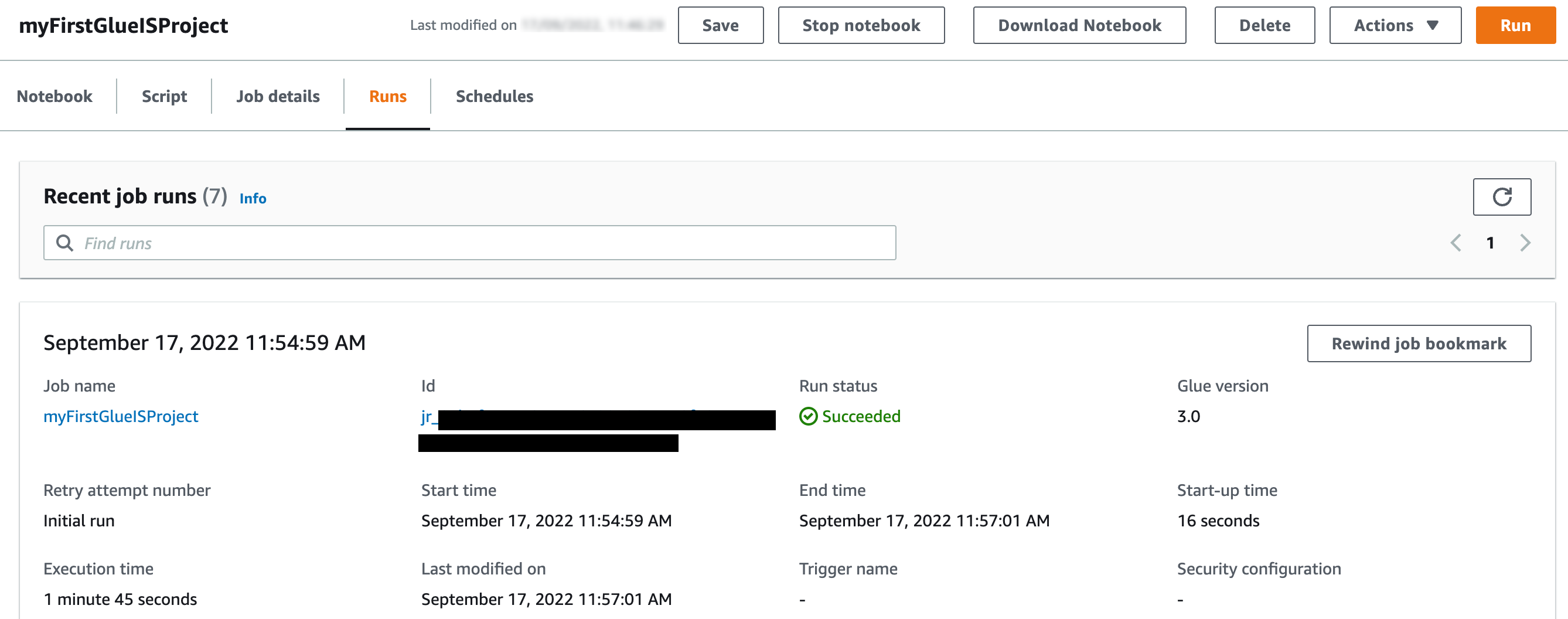
You can check its status on the Runs tab.glue interactive session job run statusThe job completed in less than 5 minutes with G1.x 3 DPUs.
  7. Let’s check the count of records in f_nyc_yellow_taxi_trip and d_nyc_taxi_zone_lookup tables in Amazon Redshift:
    SELECT 'f_nyc_yellow_taxi_trip' AS table_name, COUNT(1) FROM "public"."f_nyc_yellow_taxi_trip"
    UNION ALL
    SELECT 'd_nyc_taxi_zone_lookup' AS table_name, COUNT(1) FROM "public"."d_nyc_taxi_zone_lookup";

    redshift count query output

    With job bookmarks enabled, even if you run the job again with no new files in corresponding folders in the S3 bucket, it doesn’t process the same files again. The following screenshot shows a subsequent job run in my environment, which completed in less than 2 minutes because there were no new files to process.

    glue interactive session job re-run

    Now let’s schedule the job.

  8. On the Schedules tab, choose Create schedule.
    glue interactive session create schedule
  9. For Name¸ enter a name (for example, myFirstGlueISProject-testSchedule).
  10. For Frequency, choose Custom.
  11. Enter a cron expression so the job runs every Monday at 6:00 AM.
  12. Add an optional description.
  13. Choose Create schedule.
    glue interactive session add schedule

The schedule has been saved and activated. You can edit, pause, resume, or delete the schedule from the Actions menu.

glue interactive session schedule action

Clean up

To avoid incurring future charges, delete the AWS resources you created.

  • Delete the AWS Glue job (myFirstGlueISProject for this post).
  • Delete the Amazon S3 objects and bucket (my-first-aws-glue-is-project-<random number> for this post).
  • Delete the AWS IAM policies and roles (AWSGlueInteractiveSessionPassRolePolicy, AmazonS3Access-MyFirstGlueISProject and AWSGlueServiceRole-GlueIS).
  • Delete the Amazon Redshift tables (f_nyc_yellow_taxi_trip and d_nyc_taxi_zone_lookup).
  • Delete the AWS Glue JDBC Connection (redshiftServerless).
  • Also delete the self-referencing Redshift Serverless security group, and Amazon S3 endpoint (if you created it while following the steps for this post).

Conclusion

In this post, we demonstrated how to do the following:

  • Set up an AWS Glue Jupyter notebook with interactive sessions
  • Use the notebook’s magics, including the AWS Glue connection onboarding and bookmarks
  • Read the data from Amazon S3, and transform and load it into Amazon Redshift Serverless
  • Configure magics to enable job bookmarks, save the notebook as an AWS Glue job, and schedule it using a cron expression

The goal of this post is to give you step-by-step fundamentals to get you going with AWS Glue Studio Jupyter notebooks and interactive sessions. You can set up an AWS Glue Jupyter notebook in minutes, start an interactive session in seconds, and greatly improve the development experience with AWS Glue jobs. Interactive sessions have a 1-minute billing minimum with cost control features that reduce the cost of developing data preparation applications. You can build and test applications from the environment of your choice, even on your local environment, using the interactive sessions backend.

Interactive sessions provide a faster, cheaper, and more flexible way to build and run data preparation and analytics applications. To learn more about interactive sessions, refer to Job development (interactive sessions), and start exploring a whole new development experience with AWS Glue. Additionally, check out the following posts to walk through more examples of using interactive sessions with different options:


About the Authors

Vikas blog picVikas Omer is a principal analytics specialist solutions architect at Amazon Web Services. Vikas has a strong background in analytics, customer experience management (CEM), and data monetization, with over 13 years of experience in the industry globally. With six AWS Certifications, including Analytics Specialty, he is a trusted analytics advocate to AWS customers and partners. He loves traveling, meeting customers, and helping them become successful in what they do.

Nori profile picNoritaka Sekiyama is a Principal Big Data Architect on the AWS Glue team. He enjoys collaborating with different teams to deliver results like this post. In his spare time, he enjoys playing video games with his family.

Gal blog picGal Heyne is a Product Manager for AWS Glue and has over 15 years of experience as a product manager, data engineer and data architect. She is passionate about developing a deep understanding of customers’ business needs and collaborating with engineers to design elegant, powerful and easy to use data products. Gal has a Master’s degree in Data Science from UC Berkeley and she enjoys traveling, playing board games and going to music concerts.

Data monetization and customer experience optimization using telco data assets: Part 2

Post Syndicated from Vikas Omer original https://aws.amazon.com/blogs/big-data/part-2-data-monetization-and-customer-experience-optimization-using-telco-data-assets/

Part 1 of this series explains the importance of building and implementing a customer experience (CX) management and data monetization strategy for telecom service providers (TSPs), and the major challenges driving these initiatives. It also includes an AWS CloudFormation template to set up a demonstration of the solution using AWS services. It covers transforming and enriching multiple datasets, and offers information about data standardization, baselining an analytics data model to marry different datasets like deep packet inspection (DPI) engine embedded Packet Switch (PS) probe, CRM, subscriptions, media, carrier, device, and network configuration management in the data warehouse with AWS Glue, AWS Lambda, and Amazon Redshift.

In this post, I demonstrate how you can enable data analysts, scientists, and advanced business users to query data from Amazon Redshift or Amazon Simple Storage Service (Amazon S3) directly. I also demonstrate configuring a simple drag-and-drop interface for self-service analytics so you can prepare and publish insights based on enriched data stored in Amazon Redshift or Amazon S3 through Amazon QuickSight.

Solution overview

The following diagram illustrates the workflow of the solution.

In part 1 of this series, we discuss the overall workflow. In this post, we focus on the following steps:

  1. Catalog the processed raw, aggregate, and dimension data in the AWS Glue Data Catalog using the DPI processed data crawler.
  2. Interactively query data directly from Amazon S3 using Amazon Athena and visualize in QuickSight.
  3. Enable self-service analytics using QuickSight to prepare and publish insights based on data residing in the Amazon Redshift cluster.

Querying data using Amazon Redshift

After creating your Amazon Redshift cluster, you can immediately run queries by using the query editor on the Amazon Redshift console. Complete the following steps:

  1. On the Amazon Redshift console, in the navigation pane, choose Clusters.

A cluster with the identifier <redshift database name>-<cloudformation stack> should be present. For this example, the cluster is cemdm-telco.

  1. Choose Editor.
  2. Enter the required credentials to connect to the Amazon Redshift query editor. (Database name, Database user, and Database password are the ones you entered while creating the CloudFormation stack.)

  1. Choose Connect to database.

Upon successful authentication, you’re directed to the query editor.

  1. Run a few queries to check if data is in the tables.

In the following code, <table-name> is the Amazon Redshift table name:

select count(1) from cemdm.<table-name>;

The following query extracts the number of unique subscriber count by age group with Apple devices browsing retail domain websites or apps in or around shopping malls. You can also extract the list of subscribers and micro-segment them by consumption (total data volume) or by adding KPIs like recency and frequency.

select 
  dcd.age_range, 
  count(distinct f.customer_id)as "Unique Subs Count"
from 
  cemdm.f_daily_dpi f
inner join cemdm.d_customer_demographics dcd on f.customer_id = dcd.customer_id
inner join cemdm.d_tac dt on f.tac_code = dt.tac_sid
inner join cemdm.d_device dd on dt.device_sid = dd.device_sid
inner join cemdm.d_dpi_dictionary ddd on f.protocol_id = ddd.app_id
inner join cemdm.d_location dl on f.location_id = dl.location_id
where 
  dd.device_manufacturer = 'Apple' 
and ddd.media_category = 'Retail' 
and location_tier_4 ilike '%mall%'
group by 1 
order by 2 desc;

The following screenshot shows the output.

Unloading processed and enriched data from Amazon Redshift to Amazon S3

Amazon Redshift also includes Amazon Redshift Spectrum, which allows you to directly run SQL queries against exabytes of unstructured data in Amazon S3 data lakes. No loading or transformation is required, and you can use open data formats, including Avro, CSV, Ion, JSON, ORC, and Parquet. Amazon Redshift Spectrum automatically scales query compute capacity based on the data being retrieved, so queries against Amazon S3 run quickly, regardless of dataset size.

Amazon Redshift Spectrum gives you the freedom to store your data where you want, in the format you want, and have it available for processing when you need it. This is particularly helpful if you need to offload cold or historical data on Amazon Redshift to Amazon S3 in open data format. You can still access this data through Amazon Redshift via Amazon Redshift Spectrum plus any other application.

TSP data assets also include a lot of unstructured event data. This data is transient, and only valuable for a short amount of time. Therefore, you can leave it on Amazon S3 and access it from Amazon Redshift directly through Amazon Redshift Spectrum. You can use a lake house architecture approach, where hot, mostly static, and corporate data is in the warehouse, and the events data is in the data lake.

Alternatively, you can analyze data on Amazon S3 using Athena.

  1. Use the queries in the following table (in the Unload Statement column) in the Amazon Redshift query editor to unload data from Amazon Redshift to Amazon S3. For instructions, see Unloading data to Amazon S3. Provide the following information:
    • <aws-stack-name> – The name of the CloudFormation stack
    • <aws-region> – The Region in which you deployed the stack (for example, us-east-1)
    • <s3-bucket-name> – The bucket that you created while deploying the stack
    • <aws-account-id> – The AWS account ID in which you deployed the stack
    • <table-name> – The name of the Amazon Redshift table
Amazon Redshift Table Unload Statement

f_raw_dpi

f_hourly_dpi

unload ('select * from  cemdm.<table-name>') 
       to 's3://<s3-bucket-name>/dpi/processed/<table-name>/' 
       iam_role 'arn:aws:iam::<aws-account-id>:role /RedshiftBasicCustom-<aws-region>-<aws-stack-name>' 
       ALLOWOVERWRITE
       PARQUET 
       PARTITION BY (date_id, hour_id);

f_daily_dpi
unload ('select * from  cemdm.<table-name>') 
       to 's3://<s3-bucket-name>/dpi/processed/f_daily_dpi/' 
       iam_role 'arn:aws:iam::<aws-account-id>:role/RedshiftBasicCustom-<aws-region>-<aws-stack-name>' 
       ALLOWOVERWRITE
       PARQUET 
       PARTITION BY (date_id);

d_customer_demographics

d_device

d_dpi_dictionary

d_location

d_operator_plmn

d_tac

d_tariff_plan

d_tariff_plan_desc

unload ('select * from  cemdm.<table-name>') 
   to 's3://<s3-bucket-name>/dpi/processed/<table-name>/' 
       iam_role 'arn:aws:iam::<aws-account-id>:role /RedshiftBasicCustom-<aws-region>-<aws-stack-name>' 
       ALLOWOVERWRITE
       PARQUET;

Alternatively, you can copy the Amazon Redshift AWS Identity and Access Management (IAM) role ARN to unload data to Amazon S3 from the console under the cluster’s properties.

  1. Verify that the data has been unloaded to Amazon S3 under <s3-bucket-name>/dpi/processed/.
  2. On the AWS Glue console, in the navigation pane, choose Crawlers.
  3. Select DPIProcessedDataCrawler.
  4. Choose Run crawler.

  1. Wait for the crawler to show the status Stopping.

The tables added against the DPIProcessedDataCrawler crawlers should show 11.

  1. Under Databases, choose Tables.
  2. Verify the following 11 tables are created under the cemdm database:
    • processed_f_raw_dpi
    • processed_f_hourly_dpi
    • processed_f_daily_dpi
    • processed_d_customer_demographics
    • processed_d_device
    • processed_d_dpi_dictionary
    • processed_d_location
    • processed_d_operator_plmn
    • processed_d_tac
    • processed_d_tariff_plan
    • processed_d_tariff_plan_desc

Visualizing data using QuickSight

QuickSight is a business analytics service you can use to build visualizations, perform one-time analysis, and get business insights from your data. For more information, see What Is Amazon QuickSight?

To connect QuickSight to Amazon Redshift as your data source, complete the following steps:

  1. Create a private connection from Amazon QuickSight to an Amazon Redshift cluster.

These steps involve creating a new private subnet that the CloudFormation stack already created. Use the private subnet that isn’t used by Amazon Redshift cluster for your QuickSight connection.

QuickSight provides out-of-the-box integration with Amazon Redshift, making it simple to query and visualize your Redshift data. For more information, see Creating a Dataset from an Autodiscovered Amazon Redshift Cluster or Amazon RDS Instance.

  1. For Schema, choose cdmdm.
  2. For Tables, select f_daily_dpi.
  3. Choose Edit/Preview data.

  1. Add data and prepare the following table relationships in the Data Prep Use the information provided to create the relationships between different tables:
Table A Name Table A Attribute Join Type Table B Name Table B Attribute
f_daily_dpi customer_id LEFT d_tariff_plan customer_id
f_daily_dpi tac_code INNER d_tac tac_sid
f_daily_dpi sgsn_plmn_sid INNER d_operator_plmn plmn_sid
f_daily_dpi location_id LEFT d_location location_id
f_daily_dpi protocol_id INNER d_dpi_dictionary app_id
f_daily_dpi customer_id LEFT d_customer_demographics customer_id
d_tariff_plan tariff_plan_id INNER d_tariff_plan_desc tariff_plan_id
d_tac device_sid INNER d_device device_sid

You can join d_operator_plmn with sgsn_plmn_sid and home_plmn_sid, but because the sample data only contains home subscriber data, a second join of f_raw_dpi data with d_operator_plmn on home_plmn_sid and plmn_sid is not present in the given relationship of tables.

The following screenshot shows the table relationships.

  1. Name your analysis CEMDM.
  2. Choose Save & visualize.

The following screenshots demonstrate a few QuickSight analyses created from the dataset we created. For more information about creating analyses in QuickSight, see Working with Analyses. You can divide all analyses across all the available attributes. We use the use case from part 1 of this series.

The following screenshot shows visualizations of user demographics on the Demographics tab.

The following screenshot shows visualizations of user interest on the Interest Analysis tab.

The following screenshot shows visualizations of user locations on the Location tab.

The following screenshot shows visualizations of device information on the Device tab.

The following screenshot shows visualizations of subscription information on the Subscriptions tab.

The following screenshot shows visualizations of roaming users on the Roaming tab.

The following screenshot shows visualizations on the Sub Details tab. You can drill down to subscriber-level details from any dashboard across any dimension or apply global-level filters to narrow down the desired segment.

You can also build these reports using Athena as a data connector. QuickSight provides out-of-the-box integration with Athena, which lets you run SQL queries on top of the metadata in your AWS Glue Data Catalog. For more information, see Creating a Dataset Using Amazon Athena Data.

You can also use Amazon Redshift metadata as a business glossary and visualize it using QuickSight with the following custom SQL:

SELECT * FROM (
  select 
    n.nspname as "Schema",c1.relname as "Table Name", c.attname as "Column Name", 'Attribute' as "Type",
    c.attnum as "Ordinal Position",typnotnull as "Is Not Null",typdefault as "Default Value", t.typname as "Data Type",
    split_part(d.description,'|',1) as "Category", 
    split_part(d.description,'|',2) as "Source",
    split_part(d.description,'|',3) as "Transient/Derived",
    split_part(d.description,'|',4) as "Is PII",
    split_part(d.description,'|',5) as "Is Business Sensitive",
    split_part(d.description,'|',6) as "Description"  
  from pg_catalog.pg_attribute c
  inner join pg_class c1 on c.attrelid=c1.oid
  inner JOIN pg_type t on t.oid=c.atttypid
  inner join pg_catalog.pg_namespace n on c1.relnamespace=n.oid
  inner join pg_catalog.pg_description d on d.objoid=c1.oid AND c.attnum = d.objsubid
  where n.nspname='cemdm' and c.attnum > 0
  UNION ALL
  select 
    pn.nspname as "Schema",pc.relname "Table Name",null as "Column Name", 'Table' as "Type", 
    null as "Ordinal Position",null as "Is Not Null",null as "Default Value",null as "Data Type",
    split_part(pd.description,'|',1) as "Category", 
    split_part(pd.description,'|',2) as "Source",
    split_part(pd.description,'|',3) as "Transient/Derived",
    split_part(pd.description,'|',4) as "Is PII",
    split_part(pd.description,'|',5) as "Is Business Sensitive",
    split_part(pd.description,'|',6) as "Description"
  from pg_catalog.pg_description pd 
  inner join pg_class pc on pd.objoid = pc.oid
  inner join pg_catalog.pg_namespace pn on pc.relnamespace = pn.oid
  where pn.nspname = 'cemdm' and pd.objsubid = 0
) x
order by "Table Name", nvl("Ordinal Position",0);

The following screenshot shows a sample visualization which you can build on QuickSight.

For more information about running custom Amazon Redshift SQL using Amazon QuickSight, see Using the Query Editor.

QuickSight allows creating template from existing analysis. You can use the resulting template to create a dashboard. For more information, see Evolve your analytics with Amazon QuickSight’s new APIs and theming capabilitiesYou can also embed QuickSight dashboards into your own apps, websites, and wikis without the need to provision and manage users (readers) in QuickSight. For more information, see New in Amazon QuickSight – session capacity pricing for large scale deployments, embedding in public websites, and developer portal for embedded analytics.”

Cleaning up

To avoid incurring future charges, delete the resources you created. Manually delete anything created outside of the CloudFormation stack and then the stack itself.

Conclusion

In this post, I demonstrated how data analysts, data scientists, and advanced business users can easily query multiple data sources and generate actionable insights including user interest profiles, segments, and micro-segments. Downstream systems like campaign management systems, customer care portals, and customer-facing applications; internal teams like retention, marketing, CX, and network; and workloads like machine learning can greatly benefit from the insights generated from this solution. You can automate these insights and integrate them with northbound systems, and trigger them based on a schedule or an event.

I also demonstrated how business users are empowered with self-service analytics to help them perform data exploration and publish ready-made insights in the form of dashboards. You can also create stories to drive data-heavy conversations based on enriched data stored in Amazon Redshift or Amazon S3.

Perceiving customer behavior across multiple touchpoints is the key for any business to thrive. And the essence of this solution is to capitalize on data and drive CX and monetization initiatives holistically across your organization. This framework allows you to accelerate your journey towards improving CX and generating new revenue streams by using existing data assets.

You can progressively augment this solution by adding additional data sources to evolve into a customer data platform hosting 360° profiles of individual subscribers correlated from multiple data sources. This solution can further support new and existing marketing, partnerships, loyalty, retention, network planning, and network optimization initiatives to drive revenue growth and improve profitability while keeping subscribers happy and loyal. It also helps you define an organization-wide standard for data visualization, self-service analytics, metadata discovery, and data marketplace.

For more ways to expand this solution, consider the following services:

  • AWS Data Exchange makes it easy to find, subscribe to, and use third-party data in the cloud. You can merge it with in-house data assets to span existing insights across multiple domains.
  • Amazon Pinpoint is a flexible and scalable outbound and inbound marketing communications service. You can connect with customers over channels like email, SMS, push, or voice. You can segment and micro-segment your campaign audience for the right customer and personalize your messages with the right content.

As always, AWS welcomes feedback. This is a wide-open space to explore, so reach out to us if you want to dive deep into understanding how you can build this solution and more on AWS. Please submit comments or questions in the comments section.


About the Author

Vikas Omer is an analytics specialist solutions architect at Amazon Web Services. Vikas has a strong background in analytics, customer experience management (CEM) and data monetization, with over 11 years of experience in the telecommunications industry globally. With six AWS Certifications, including Analytics Specialty, he is a trusted analytics advocate to AWS customers and partners. He loves traveling, meeting customers, and helping them become successful in what they do.

Data monetization and customer experience optimization using telco data assets: Part 1

Post Syndicated from Vikas Omer original https://aws.amazon.com/blogs/big-data/part-1-data-monetization-and-customer-experience-optimization-using-telco-data-assets/

The landscape of the telecommunications industry is changing rapidly. For telecom service providers (TSPs), revenue from core voice and data services continues to shrink due to regulatory pressure and emerging OTT players that offer an attractive alternative. Despite increasing demand from customers for bandwidth, speed, and efficiency, TSPs are finding that ROI from implementing new access technologies like 5G are unsubstantial.

To overcome the risk of being relegated to a utility or dumb pipe, TSPs today are looking to diversify, adopting alternative business models to generate new revenue streams.

In recent times, adopting customer experience (CX) and data monetization initiatives has been a key theme across all industries. Although many Tier-1 TSPs are leading this transformation by using new technologies to improve CX and improve profitability, many TSPs have yet to embark on this challenging but rewarding journey.

Building and implementing a CX management and data monetization strategy

Data monetization is often misunderstood as making dollars by selling data, but what it really means is to drive revenue by increasing the top line or the bottom line. It can be tangible or intangible, internal or external, or by making use of data assets.

According to Gartner, most data and analytics leaders are looking to increase investments in business intelligence (BI) and analytics (see the following study results).

The preceding visualization is from “The 2019 CIO Agenda: Securing a New Foundation for Digital Business”, published October 15, 2018.

Although the external monetization opportunities are limited due to strict regulations, a plethora of opportunities exist for TSPs to monetize data both internally (regulated but much less compared to external) and externally via a marketplace (highly regulated). If TSPs can shift their mindsets from selling data to focus on using data insights for monetization and improving CX, they can adopt a significant number of use cases to realize an immediate positive impact.

Tapping and utilizing insights around customer behavior acts like a Swiss Army Knife for businesses. You can use these insights to drive CX, hyper-personalization and localization, micro-segmentation, subscriber retention, loyalty and rewards programs, network planning and optimization, internal and external data monetization, and more. The following are some use cases that can be driven using CX and data monetization strategies:

  • Segmentation/micro-segmentation (cross-sell, up-sell, targeted advertising, enhanced market locator); for example:
    • Identify targets for consuming baby products or up-selling a kids-related TV channel
    • Identify females in the age range of 18-35 to target for high-end beauty products or apparels

You can build hundreds of such segments.

  • Personalized loyalty and reward programs (incentivize customers with what they like). For example, movie tickets or discounts for a movie lover, or food coupons and deals for a food lover.
  • CX-driven network optimization (allocate more resources to streaming hotspots with high-value customers).
  • Identifying potential partners for joint promotions. For example, bundling device offers with a music app subscription.
  • Hyper-personalization. For example, personalized recommendations for on-portal apps and websites.
  • Next best action and next best offer. For example, intelligent bundling and packaging of offerings.

Challenges with driving CX and data monetization

In this digital era, TSPs consider data analytics a strategic pillar in their quest to evolve into a true data-driven organization. Although many TSPs are harnessing the power of data to drive and improve CX, there are technological gaps and challenges to baseline and formulate internal and external data monetization strategies. Some of these challenges include:

  • Non-overlapping technology investments for CX and data monetization due to misaligned business and IT initiatives
  • Huge CAPEX requirements to process massive volumes of data
  • Inability to unearth hidden insights due to siloed data initiatives
  • Inability to marry various datasets together due to missing pieces around data standardization techniques
  • Lack of user-friendly tools and techniques to discover, ingest, process, correlate, analyze, and consume the data
  • Inability to experiment and innovate with agility and low cost

In this two-part series, I demonstrate a working solution with an AWS CloudFormation template for how a TSP can use existing data assets to generate new revenue streams and improve and personalize CX using AWS services. I also include key pieces of information around data standardization, baselining an analytics data model to marry different datasets in the data warehouse, self-service analytics, metadata search, and media dictionary framework.

In this post, you deploy the stack using a CloudFormation template and follow simple steps to transform, enrich, and bring multiple datasets together so that they can be correlated and queried.

In part 2, you learn how advanced business users can query enriched data and derive meaningful insights using Amazon Redshift and Amazon Redshift Spectrum or Amazon Athena, enable self-service analytics for business users, and publish ready-made dashboards via Amazon QuickSight.

Solution overview

The main ingredient of this solution is Packet Switch (PS) probe data embedded with a deep packet inspection (DPI) engine, which can reveal a lot of information about user interests and usage behavior. This data is transformed and enriched with DPI media and device dictionaries, along with other standard telco transformations to deduce insights, profile and micro-segment subscribers. Enriched data is made available along with other transformed dimensional attributes (CRM, subscriptions, media, carrier, device and network configuration management) for rich slicing and dicing.

For example, the following QuickSight visualizations depict a use case to identity music lovers ages 18-55 with Apple devices. You can also generate micro-segments by capturing the top X subscribers by consumption or adding KPIs like recency and frequency.

The following diagram illustrates the workflow of the solution.

For this post, AWS CloudFormation sets up the required folder structure in Amazon Simple Storage Service (Amazon S3) and provides sample data and dictionary file. Most of the data included as part of the CloudFormation template is dummy and is as follows:

  • CRM
  • Subscription and subscription mapping
  • Network 3G & 4G configuration management
  • Operator PLMN
  • DPI and device dictionary
  • PS probe data

Descriptions of all the input datasets and attributes are available with AWS Glue Data Catalog tables and as part of Amazon Redshift metadata for all tables in Amazon Redshift.

The workflow for this post includes the following steps:

  1. Catalog all the files in the AWS Glue Data Catalog using the following AWS Glue data crawlers:
    1. DPI data crawler (to crawl incoming PS probe DPI data)
    2. Dimension data crawler (to crawl all dimension data)
  2. Update attribute descriptions in the Data Catalog (this step is optional).
  3. Create Amazon Redshift schema, tables, procedures, and metadata using an AWS Lambda
  4. Process each data source file using separate AWS Glue Spark jobs. These jobs enrich, transform, and apply business filtering rules before ingesting data into an Amazon Redshift cluster.
  5. Trigger Amazon Redshift hourly and daily aggregation procedures using Lambda functions to aggregate data from the raw table into hourly and daily tables.

Part 2 includes the following steps:

  1. Catalog the processed raw, aggregate, and dimension data in the Data Catalog using the DPI processed data crawler.
  2. Interactively query data directly from Amazon S3 using Amazon Athena.
  3. Enable self-service analytics using QuickSight to prepare and publish insights based on data residing in the Amazon Redshift cluster.

The workflow can change depending on the complexity of the environment and your use case, but the fundamental idea remains the same. For example, your use case could be processing PS probe DPI data in real time rather than in batch mode, keeping hot data in Amazon Redshift, storing cold and historical data on Amazon S3, or archiving data in Amazon S3 Glacier for regulatory compliance. Amazon S3 offers several storage classes designed for different use cases. You can move the data among these different classes based on Amazon S3 lifecycle properties. For more information, see Amazon S3 Storage Classes.

Prerequisites

For this walkthrough, you should have the following prerequisites:

For more information about AWS Regions and where AWS services are available, see Region Table.

Creating your resources with AWS CloudFormation

To get started, create your resources with the following CloudFormation stack.

  1. Click the Launch Stack button below:
  2. Leave the parameters at their default, with the following exceptions:
    1. Enter RedshiftPassword and S3BucketNameParameter parameters, which aren’t populated by default.
    2. An Amazon S3 bucket name is globally unique, so enter a unique bucket name for S3BucketNameParameter.

The following screenshot shows the parameters for our use case.

  1. Choose Next.
  2. Select I acknowledge that AWS CloudFormation might create IAM resources with custom names.
  3. Choose Create stack.

It takes approximately 10 minutes to deploy the stack. For more information about the key resources deployed through the stack, see Data Monetization and Customer Experience(CX)Optimization using telco data assets: Amazon CloudFormation stack details. You can view all the resources on the AWS CloudFormation console. For instructions, see Viewing AWS CloudFormation stack data and resources on the AWS Management Console.

The CloudFormation stack we provide in this post serves as a baseline and is not a production-grade solution.

Building a Data Catalog using AWS Glue

You start by discovering sample data stored on Amazon S3 through an AWS Glue crawler. For more information, see Populating the AWS Glue Data Catalog. To catalog data, complete the following steps:

  1. On the AWS Glue console, in the navigation pane, choose Crawlers.
  2. Select DPIRawDataCrawler and choose Run crawler.
  3. Select DimensionDataCrawler and choose Run crawler.
  4. Wait for the crawlers to show the status Stopping.

The tables added against the DimensionDataCrawler and DPIRawDataCrawler crawlers should show 9 and 1, respectively.

  1. In the navigation pane, choose Tables.
  2. Verify the following 10 tables are created under the cemdm database:
    • d_crm_demographics
    • d_device
    • d_dpi_dictionary
    • d_network_cm_3g
    • d_network_cm_4g
    • d_operator_plmn
    • d_tac
    • d_tariff_plan
    • d_tariff_plan_desc
    • raw_dpi_incoming

Updating attribute descriptions in the Data Catalog

The AWS Glue Data Catalog has a comment field to store the metadata under each table in the AWS Glue database. Anybody who has access to this database can easily understand attributes coming from different data sources through metadata provided in the comment field. The CloudFormation stack includes a CSV file that contains a description of all the attributes from the source files. This file is used to update the comment field for all the Data Catalog tables this stack deployed. This step is not mandatory to proceed with the workflow. However, if you want to update the comment field against each table, complete the following steps:

  1. On the Lambda console, in the navigation pane, choose Functions.
  2. Choose the GlueCatalogUpdate
  3. Configure a test event by choosing Configure test events.
  4. For Event name, enter Test.
  5. Choose Create.
  6. Choose Test.

You should see a message that the test succeeded, which implies that the Data Catalog attribute description is complete.

Attributes of the table under the Data Catalog database should now have descriptions in the Comment column. For example, the following screenshot shows the d_operator_plmn table.

Creating Amazon Redshift schema, tables, procedures, and metadata

To create schema, tables, procedures, and metadata in Amazon Redshift, complete the following steps:

  1. On the Lambda console, in the navigation pane, choose Functions.
  2. Choose the RedshiftDDLCreation
  3. Choose Configure test events.
  4. For Event name, enter Test.
  5. Choose Create.
  6. Choose Test.

You should see a message that the test succeeded, which means that the schema, table, procedures, and metadata generation is complete.

Running AWS Glue ETL jobs

AWS Glue provides the serverless, scalable, and distributed processing capability to transform and enrich your datasets. To run AWS Glue extract, transform, and load (ETL) jobs, complete the following steps:

  1. On the AWS Glue console, in the navigation pane, choose Jobs.
  2. Select the following jobs (one at a time) and choose Run job from Action
    • d_customer_demographics
    • d_device
    • d_dpi_dictionary
    • d_location
    • d_operator_plmn
    • d_tac
    • d_tariff_plan
    • d_tariff_plan_desc
    • f_dpi_enrichment

You can run all these jobs in parallel.

All dimension data jobs should finish successfully within 3 minutes, and the fact data enrichment job should finish within 5 minutes.

  1. Verify the jobs are complete by selecting each job and checking Run status on the History tab.

Aggregating hourly and daily DPI data in Amazon Redshift

To aggregate hourly and daily sample data in Amazon Redshift using Lambda functions, complete the following steps:

  1. On the Lambda console, in the navigation pane, choose Functions.
  2. Choose the RedshiftDPIHourlyAgg function.
  3. Choose Configure test events.
  4. For Event name, enter Test.
  5. Choose Create.
  6. Choose Test.

You should see a message that the test succeeded, which means that hourly aggregation is complete.

  1. In the navigation pane, choose Functions.
  2. Choose the RedshiftDPIDailyAgg function.
  3. Choose Configure test events.
  4. For Event name, enter Test.
  5. Choose Create.
  6. Choose Test.

You should see a message that the test succeeded, which means that daily aggregation is complete.

Both hourly and daily Lambda functions are hardcoded with the date and hour to aggregate the sample data. To make them generic, there are a few commented lines of code that need to be uncommented and a few lines to be commented. Both functions are also equipped with offset parameters to decide how far back in time you want to do the aggregations. However, this isn’t required for this walkthrough.

You can schedule these functions with CloudWatch. However, this is not required for this walkthrough.

So far, we have completed the following:

  1. Deployed the CloudFormation stack.
  2. Cataloged sample raw data by running DimensionDataCrawler and DPIRawDataCrawler AWS Glue crawlers.
  3. Updated attribute descriptions in the AWS Glue Data Catalog by running the GlueCatalogUpdate Lambda function.
  4. Created Amazon Redshift schema, tables, stored procedures, and metadata through the RedshiftDDLCreation Lambda function.
  5. Ran all AWS Glue ETL jobs to transform raw data and load it into their respective Amazon Redshift tables.
  6. Aggregated hourly and daily data from enriched raw data into hourly and daily Amazon Redshift tables by running the RedshiftDPIHourlyAgg and RedshiftDPIDailyAgg Lambda functions.

Cleaning up

If you don’t plan to proceed to the part 2 of this series, and want to avoid incurring future charges, delete the resources you created by deleting the CloudFormation stack.

Conclusion

In this post, I demonstrated how you can easily transform, enrich, and bring multiple telco datasets together in an Amazon Redshift data warehouse cluster. You can correlate these datasets to produce multi-dimensional insights from several angles, like subscriber, network, device, subscription, roaming, and more.

In part 2 of this series, I demonstrate how you can enable data analysts, scientists, and advanced business users to query data from Amazon Redshift or Amazon S3 directly.

As always, AWS welcomes feedback. This is a wide space to explore, so reach out to us if you want a deep dive into building this solution and more on AWS. Please submit comments or questions in the comments section.


About the Author

Vikas Omer is an analytics specialist solutions architect at Amazon Web Services. Vikas has a strong background in analytics, customer experience management (CEM), and data monetization, with over 11 years of experience in the telecommunications industry globally. With six AWS Certifications, including Analytics Specialty, he is a trusted analytics advocate to AWS customers and partners. He loves traveling, meeting customers, and helping them become successful in what they do.