Tag Archives: Jupyter Notebook

Investigation of a Workbench UI Latency Issue

Post Syndicated from Netflix Technology Blog original https://netflixtechblog.com/investigation-of-a-workbench-ui-latency-issue-faa017b4653d

By: Hechao Li and Marcelo Mayworm

With special thanks to our stunning colleagues Amer Ather, Itay Dafna, Luca Pozzi, Matheus Leão, and Ye Ji.

Overview

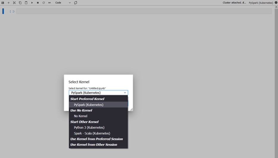
At Netflix, the Analytics and Developer Experience organization, part of the Data Platform, offers a product called Workbench. Workbench is a remote development workspace based on Titus that allows data practitioners to work with big data and machine learning use cases at scale. A common use case for Workbench is running JupyterLab Notebooks.

Recently, several users reported that their JupyterLab UI becomes slow and unresponsive when running certain notebooks. This document details the intriguing process of debugging this issue, all the way from the UI down to the Linux kernel.

Symptom

Machine Learning engineer Luca Pozzi reported to our Data Platform team that their JupyterLab UI on their workbench becomes slow and unresponsive when running some of their Notebooks. Restarting the ipykernel process, which runs the Notebook, might temporarily alleviate the problem, but the frustration persists as more notebooks are run.

Quantify the Slowness

While we observed the issue firsthand, the term “UI being slow” is subjective and difficult to measure. To investigate this issue, we needed a quantitative analysis of the slowness.

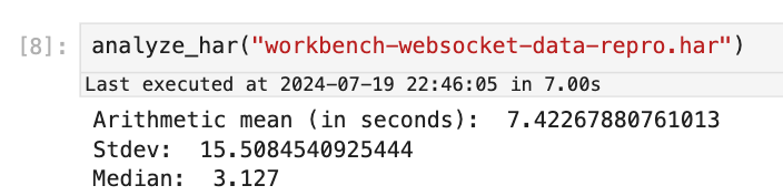
Itay Dafna devised an effective and simple method to quantify the UI slowness. Specifically, we opened a terminal via JupyterLab and held down a key (e.g., “j”) for 15 seconds while running the user’s notebook. The input to stdin is sent to the backend (i.e., JupyterLab) via a WebSocket, and the output to stdout is sent back from the backend and displayed on the UI. We then exported the .har file recording all communications from the browser and loaded it into a Notebook for analysis.

Using this approach, we observed latencies ranging from 1 to 10 seconds, averaging 7.4 seconds.

Blame The Notebook

Now that we have an objective metric for the slowness, let’s officially start our investigation. If you have read the symptom carefully, you must have noticed that the slowness only occurs when the user runs certain notebooks but not others.

Therefore, the first step is scrutinizing the specific Notebook experiencing the issue. Why does the UI always slow down after running this particular Notebook? Naturally, you would think that there must be something wrong with the code running in it.

Upon closely examining the user’s Notebook, we noticed a library called pystan , which provides Python bindings to a native C++ library called stan, looked suspicious. Specifically, pystan uses asyncio. However, because there is already an existing asyncio event loop running in the Notebook process and asyncio cannot be nested by design, in order for pystan to work, the authors of pystan recommend injecting pystan into the existing event loop by using a package called nest_asyncio, a library that became unmaintained because the author unfortunately passed away.

Given this seemingly hacky usage, we naturally suspected that the events injected by pystan into the event loop were blocking the handling of the WebSocket messages used to communicate with the JupyterLab UI. This reasoning sounds very plausible. However, the user claimed that there were cases when a Notebook not using pystan runs, the UI also became slow.

Moreover, after several rounds of discussion with ChatGPT, we learned more about the architecture and realized that, in theory, the usage of pystan and nest_asyncio should not cause the slowness in handling the UI WebSocket for the following reasons:

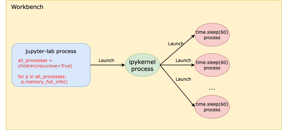
Even though pystan uses nest_asyncio to inject itself into the main event loop, the Notebook runs on a child process (i.e., the ipykernel process) of the jupyter-lab server process, which means the main event loop being injected by pystan is that of the ipykernel process, not the jupyter-server process. Therefore, even if pystan blocks the event loop, it shouldn’t impact the jupyter-lab main event loop that is used for UI websocket communication. See the diagram below:

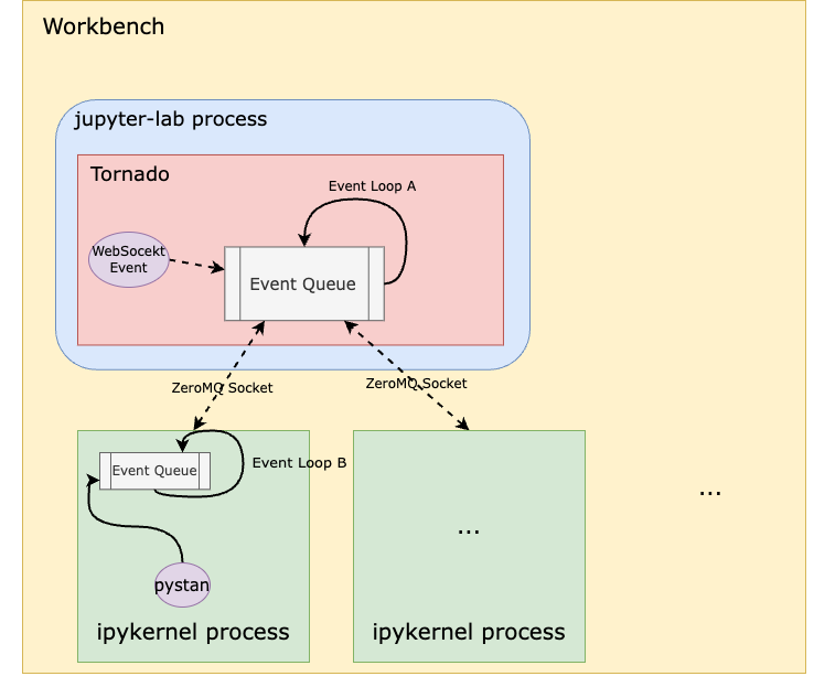
In other words, pystan events are injected to the event loop B in this diagram instead of event loop A. So, it shouldn’t block the UI WebSocket events.

You might also think that because event loop A handles both the WebSocket events from the UI and the ZeroMQ socket events from the ipykernel process, a high volume of ZeroMQ events generated by the notebook could block the WebSocket. However, when we captured packets on the ZeroMQ socket while reproducing the issue, we didn’t observe heavy traffic on this socket that could cause such blocking.

A stronger piece of evidence to rule out pystan was that we were ultimately able to reproduce the issue even without it, which I’ll dive into later.

Blame Noisy Neighbors

The Workbench instance runs as a Titus container. To efficiently utilize our compute resources, Titus employs a CPU oversubscription feature, meaning the combined virtual CPUs allocated to containers exceed the number of available physical CPUs on a Titus agent. If a container is unfortunate enough to be scheduled alongside other “noisy” containers — those that consume a lot of CPU resources — it could suffer from CPU deficiency.

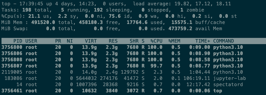
However, after examining the CPU utilization of neighboring containers on the same Titus agent as the Workbench instance, as well as the overall CPU utilization of the Titus agent, we quickly ruled out this hypothesis. Using the top command on the Workbench, we observed that when running the Notebook, the Workbench instance uses only 4 out of the 64 CPUs allocated to it. Simply put, this workload is not CPU-bound.

Blame The Network

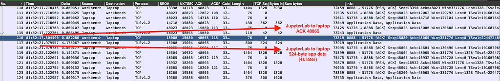
The next theory was that the network between the web browser UI (on the laptop) and the JupyterLab server was slow. To investigate, we captured all the packets between the laptop and the server while running the Notebook and continuously pressing ‘j’ in the terminal.

When the UI experienced delays, we observed a 5-second pause in packet transmission from server port 8888 to the laptop. Meanwhile, traffic from other ports, such as port 22 for SSH, remained unaffected. This led us to conclude that the pause was caused by the application running on port 8888 (i.e., the JupyterLab process) rather than the network.

The Minimal Reproduction

As previously mentioned, another strong piece of evidence proving the innocence of pystan was that we could reproduce the issue without it. By gradually stripping down the “bad” Notebook, we eventually arrived at a minimal snippet of code that reproduces the issue without any third-party dependencies or complex logic:

import time
import os
from multiprocessing import Process

N = os.cpu_count()

def launch_worker(worker_id):
time.sleep(60)

if __name__ == '__main__':
with open('/root/2GB_file', 'r') as file:
data = file.read()
processes = []
for i in range(N):
p = Process(target=launch_worker, args=(i,))
processes.append(p)
p.start()

for p in processes:
p.join()

The code does only two things:

  1. Read a 2GB file into memory (the Workbench instance has 480G memory in total so this memory usage is almost negligible).
  2. Start N processes where N is the number of CPUs. The N processes do nothing but sleep.

There is no doubt that this is the most silly piece of code I’ve ever written. It is neither CPU bound nor memory bound. Yet it can cause the JupyterLab UI to stall for as many as 10 seconds!

Questions

There are a couple of interesting observations that raise several questions:

  • We noticed that both steps are required in order to reproduce the issue. If you don’t read the 2GB file (that is not even used!), the issue is not reproducible. Why using 2GB out of 480GB memory could impact the performance?
  • When the UI delay occurs, the jupyter-lab process CPU utilization spikes to 100%, hinting at contention on the single-threaded event loop in this process (event loop A in the diagram before). What does the jupyter-lab process need the CPU for, given that it is not the process that runs the Notebook?
  • The code runs in a Notebook, which means it runs in the ipykernel process, that is a child process of the jupyter-lab process. How can anything that happens in a child process cause the parent process to have CPU contention?
  • The workbench has 64CPUs. But when we printed os.cpu_count(), the output was 96. That means the code starts more processes than the number of CPUs. Why is that?

Let’s answer the last question first. In fact, if you run lscpu and nproc commands inside a Titus container, you will also see different results — the former gives you 96, which is the number of physical CPUs on the Titus agent, whereas the latter gives you 64, which is the number of virtual CPUs allocated to the container. This discrepancy is due to the lack of a “CPU namespace” in the Linux kernel, causing the number of physical CPUs to be leaked to the container when calling certain functions to get the CPU count. The assumption here is that Python os.cpu_count() uses the same function as the lscpu command, causing it to get the CPU count of the host instead of the container. Python 3.13 has a new call that can be used to get the accurate CPU count, but it’s not GA’ed yet.

It will be proven later that this inaccurate number of CPUs can be a contributing factor to the slowness.

More Clues

Next, we used py-spy to do a profiling of the jupyter-lab process. Note that we profiled the parent jupyter-lab process, not the ipykernel child process that runs the reproduction code. The profiling result is as follows:

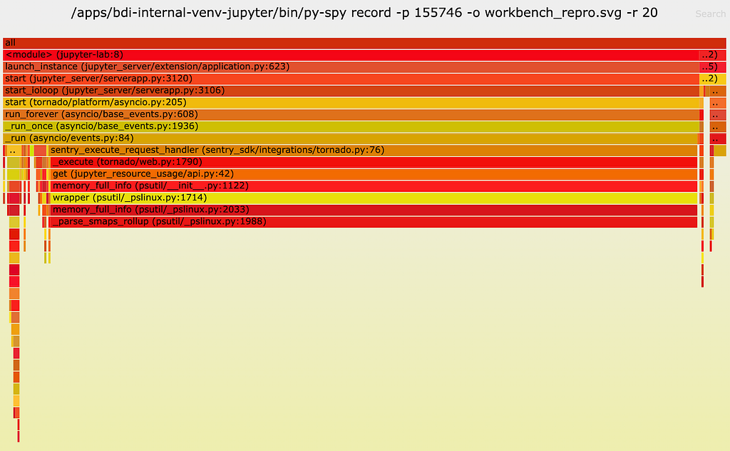
As one can see, a lot of CPU time (89%!!) is spent on a function called __parse_smaps_rollup. In comparison, the terminal handler used only 0.47% CPU time. From the stack trace, we see that this function is inside the event loop A, so it can definitely cause the UI WebSocket events to be delayed.

The stack trace also shows that this function is ultimately called by a function used by a Jupyter lab extension called jupyter_resource_usage. We then disabled this extension and restarted the jupyter-lab process. As you may have guessed, we could no longer reproduce the slowness!

But our puzzle is not solved yet. Why does this extension cause the UI to slow down? Let’s keep digging.

Root Cause Analysis

From the name of the extension and the names of the other functions it calls, we can infer that this extension is used to get resources such as CPU and memory usage information. Examining the code, we see that this function call stack is triggered when an API endpoint /metrics/v1 is called from the UI. The UI apparently calls this function periodically, according to the network traffic tab in Chrome’s Developer Tools.

Now let’s look at the implementation starting from the call get(jupter_resource_usage/api.py:42) . The full code is here and the key lines are shown below:

cur_process = psutil.Process()
all_processes = [cur_process] + cur_process.children(recursive=True)

for p in all_processes:
info = p.memory_full_info()

Basically, it gets all children processes of the jupyter-lab process recursively, including both the ipykernel Notebook process and all processes created by the Notebook. Obviously, the cost of this function is linear to the number of all children processes. In the reproduction code, we create 96 processes. So here we will have at least 96 (sleep processes) + 1 (ipykernel process) + 1 (jupyter-lab process) = 98 processes when it should actually be 64 (allocated CPUs) + 1 (ipykernel process) + 1 (jupyter-lab process) = 66 processes, because the number of CPUs allocated to the container is, in fact, 64.

This is truly ironic. The more CPUs we have, the slower we are!

At this point, we have answered one question: Why does starting many grandchildren processes in the child process cause the parent process to be slow? Because the parent process runs a function that’s linear to the number all children process recursively.

However, this solves only half of the puzzle. If you remember the previous analysis, starting many child processes ALONE doesn’t reproduce the issue. If we don’t read the 2GB file, even if we create 2x more processes, we can’t reproduce the slowness.

So now we must answer the next question: Why does reading a 2GB file in the child process affect the parent process performance, especially when the workbench has as much as 480GB memory in total?

To answer this question, let’s look closely at the function __parse_smaps_rollup. As the name implies, this function parses the file /proc/<pid>/smaps_rollup.

def _parse_smaps_rollup(self):
uss = pss = swap = 0
with open_binary("{}/{}/smaps_rollup".format(self._procfs_path, self.pid)) as f:
for line in f:
if line.startswith(b”Private_”):
# Private_Clean, Private_Dirty, Private_Hugetlb
s uss += int(line.split()[1]) * 1024
elif line.startswith(b”Pss:”):
pss = int(line.split()[1]) * 1024
elif line.startswith(b”Swap:”):
swap = int(line.split()[1]) * 1024
return (uss, pss, swap)

Naturally, you might think that when memory usage increases, this file becomes larger in size, causing the function to take longer to parse. Unfortunately, this is not the answer because:

  • First, the number of lines in this file is constant for all processes.
  • Second, this is a special file in the /proc filesystem, which should be seen as a kernel interface instead of a regular file on disk. In other words, I/O operations of this file are handled by the kernel rather than disk.

This file was introduced in this commit in 2017, with the purpose of improving the performance of user programs that determine aggregate memory statistics. Let’s first focus on the handler of open syscall on this /proc/<pid>/smaps_rollup.

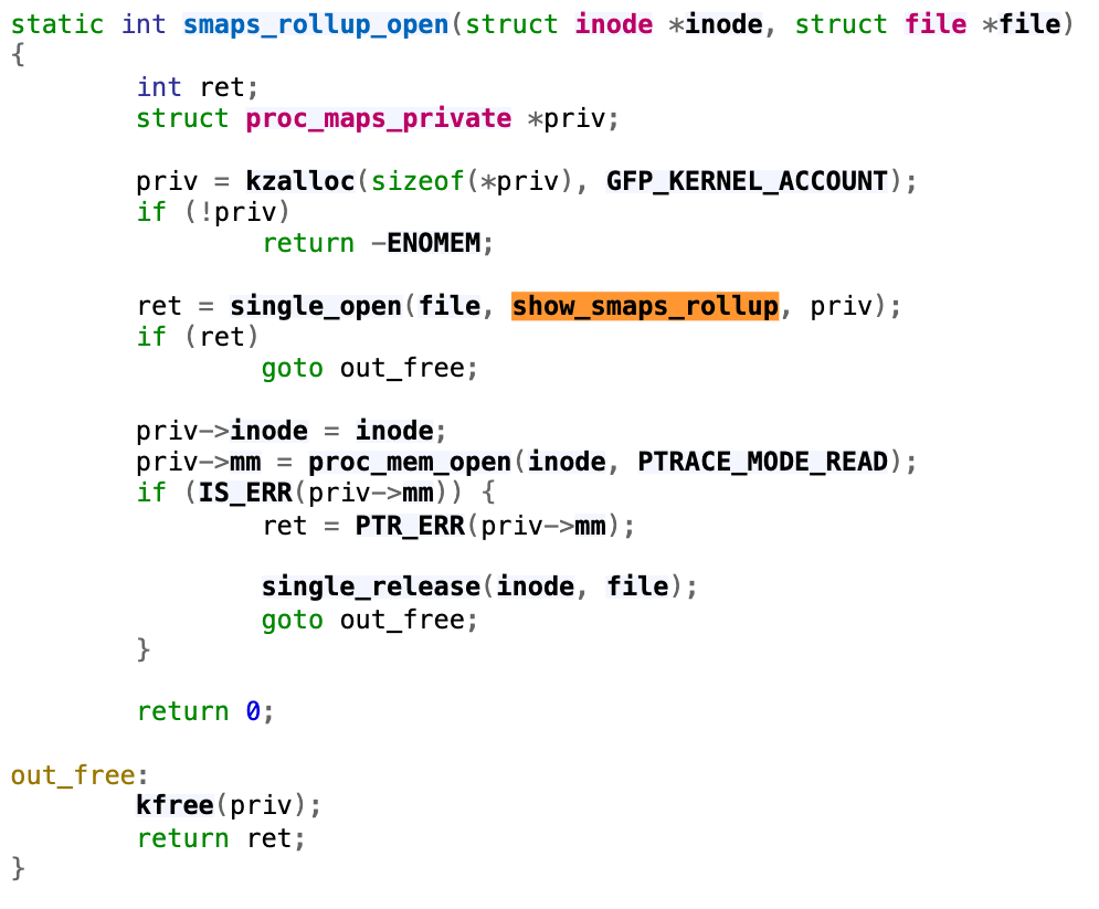
Following through the single_open function, we will find that it uses the function show_smaps_rollup for the show operation, which can translate to the read system call on the file. Next, we look at the show_smaps_rollup implementation. You will notice a do-while loop that is linear to the virtual memory area.

static int show_smaps_rollup(struct seq_file *m, void *v) {

vma_start = vma->vm_start;
do {
smap_gather_stats(vma, &mss, 0);
last_vma_end = vma->vm_end;

} for_each_vma(vmi, vma);

}

This perfectly explains why the function gets slower when a 2GB file is read into memory. Because the handler of reading the smaps_rollup file now takes longer to run the while loop. Basically, even though smaps_rollup already improved the performance of getting memory information compared to the old method of parsing the /proc/<pid>/smaps file, it is still linear to the virtual memory used.

More Quantitative Analysis

Even though at this point the puzzle is solved, let’s conduct a more quantitative analysis. How much is the time difference when reading the smaps_rollup file with small versus large virtual memory utilization? Let’s write some simple benchmark code like below:

import os

def read_smaps_rollup(pid):
with open("/proc/{}/smaps_rollup".format(pid), "rb") as f:
for line in f:
pass

if __name__ == “__main__”:
pid = os.getpid()

read_smaps_rollup(pid)

with open(“/root/2G_file”, “rb”) as f:
data = f.read()

read_smaps_rollup(pid)

This program performs the following steps:

  1. Reads the smaps_rollup file of the current process.
  2. Reads a 2GB file into memory.
  3. Repeats step 1.

We then use strace to find the accurate time of reading the smaps_rollup file.

$ sudo strace -T -e trace=openat,read python3 benchmark.py 2>&1 | grep “smaps_rollup” -A 1

openat(AT_FDCWD, “/proc/3107492/smaps_rollup”, O_RDONLY|O_CLOEXEC) = 3 <0.000023>
read(3, “560b42ed4000–7ffdadcef000 — -p 0”…, 1024) = 670 <0.000259>
...
openat(AT_FDCWD, “/proc/3107492/smaps_rollup”, O_RDONLY|O_CLOEXEC) = 3 <0.000029>
read(3, “560b42ed4000–7ffdadcef000 — -p 0”…, 1024) = 670 <0.027698>

As you can see, both times, the read syscall returned 670, meaning the file size remained the same at 670 bytes. However, the time it took the second time (i.e., 0.027698 seconds) is 100x the time it took the first time (i.e., 0.000259 seconds)! This means that if there are 98 processes, the time spent on reading this file alone will be 98 * 0.027698 = 2.7 seconds! Such a delay can significantly affect the UI experience.

Solution

This extension is used to display the CPU and memory usage of the notebook process on the bar at the bottom of the Notebook:

We confirmed with the user that disabling the jupyter-resource-usage extension meets their requirements for UI responsiveness, and that this extension is not critical to their use case. Therefore, we provided a way for them to disable the extension.

Summary

This was such a challenging issue that required debugging from the UI all the way down to the Linux kernel. It is fascinating that the problem is linear to both the number of CPUs and the virtual memory size — two dimensions that are generally viewed separately.

Overall, we hope you enjoyed the irony of:

  1. The extension used to monitor CPU usage causing CPU contention.
  2. An interesting case where the more CPUs you have, the slower you get!

If you’re excited by tackling such technical challenges and have the opportunity to solve complex technical challenges and drive innovation, consider joining our Data Platform teams. Be part of shaping the future of Data Security and Infrastructure, Data Developer Experience, Analytics Infrastructure and Enablement, and more. Explore the impact you can make with us!


Investigation of a Workbench UI Latency Issue was originally published in Netflix TechBlog on Medium, where people are continuing the conversation by highlighting and responding to this story.

Accelerate your data exploration and experimentation with the AWS Analytics Reference Architecture library

Post Syndicated from Lotfi Mouhib original https://aws.amazon.com/blogs/big-data/accelerate-your-data-exploration-and-experimentation-with-the-aws-analytics-reference-architecture-library/

Organizations use their data to solve complex problems by starting small, running iterative experiments, and refining the solution. Although the power of experiments can’t be ignored, organizations have to be cautious about the cost-effectiveness of such experiments. If time is spent creating the underlying infrastructure for enabling experiments, it further adds to the cost.

Developers need an integrated development environment (IDE) for data exploration and debugging of workflows, and different compute profiles for running these workflows. If you choose Amazon EMR for such use cases, you can use an IDE called Amazon EMR Studio for data exploration, transformation, version control, and debugging, and run Spark jobs to process large volume of data. Deploying Amazon EMR on Amazon EKS simplifies management, reduces costs, and improves performance. However, a data engineer or IT administrator needs to spend time creating the underlying infrastructure, configuring security, and creating a managed endpoint for users to connect to. This means such projects have to wait until these experts create the infrastructure.

In this post, we show how a data engineer or IT administrator can use the AWS Analytics Reference Architecture (ARA) to accelerate infrastructure deployment, saving your organization both time and money spent on these data analytics experiments. We use the library to deploy an Amazon Elastic Kubernetes (Amazon EKS) cluster, configure it to use Amazon EMR on EKS, and deploy a virtual cluster and managed endpoints and EMR Studio. You can then either run jobs on the virtual cluster or run exploratory data analysis with Jupyter notebooks on Amazon EMR Studio and Amazon EMR on EKS. The architecture below represent the infrastructure you will deploy with the AWS Analytics Reference Architecture.

cdk-emr-eks-studio-architecture

Prerequisites

To follow along, you need to have an AWS account that is bootstrapped with the AWS Cloud Development Kit (AWS CDK). For instructions, refer to Bootstrapping. The following tutorial uses TypeScript, and requires version 2 or later of the AWS CDK. If you don’t have the AWS CDK installed, refer to Install the AWS CDK.

Set up an AWS CDK project

To deploy resources using the ARA, you first need to set up an AWS CDK project and install the ARA library. Complete the following steps:

  1. Create a folder named emr-eks-app:
    mkdir emr-eks-app && cd emr-eks-app

  2. Initialize an AWS CDK project in an empty directory and run the following command:
    cdk init app --language typescript

  3. Install the ARA library:
    npm install aws-analytics-reference-architecture --save

  4. In lib/emr-eks-app.ts, import the ARA library as follows. The first line calls the ARA library, the second one defines AWS Identity and Access Management (IAM) policies:
    import * as ara from 'aws-analytics-reference-architecture'; 
    import * as iam from 'aws-cdk-lib/aws-iam';

Create and define an EKS cluster and compute capacity

To create an EMR on EKS virtual cluster, you first need to deploy an EKS cluster. The ARA library defines a construct called EmrEksCluster. The construct provisions an EKS cluster, enables IAM roles for service accounts, and deploys a set of supporting controllers like certificate manager controller (needed by the managed endpoint that is used by Amazon EMR Studio) as well as a cluster auto scaler to have an elastic cluster and save on cost when no job is submitted to the cluster.

In lib/emr-eks-app.ts, add the following line:

const emrEks = ara.EmrEksCluster.getOrCreate(this,{ 
   eksAdminRoleArn:ROLE_ARN;, 
   eksClusterName:CLUSTER_NAME;
   autoscaling: Autoscaler.KARPENTER, 
});

To learn more about the properties you can customize, refer to EmrEksClusterProps. There are two mandatory parameters in EmrEksCluster construct: The first is eksAdminRoleArn role is mandatory and is the role you use to interact with the Kubernetes control plane. This role must have administrative permissions to create or update the cluster. The second parameter is autoscaling, this parameter allows you to select the autoscaling mechanism, either Karpenter or native Kubernetes Cluster Autoscaler. In this blog we will use Karpenter and we recommend its use due to faster autoscaling, simplified node management and provisioning. Now you’re ready to define the compute capacity.

One way to define worker nodes in Amazon EKS is to use managed node groups. We use one node group called tooling, which hosts the coredns, ingress controller, certificate manager, Karpenter and any other pod that is necessary for the running EMR on EKS jobs or ManagedEndpoint. We also define default Karpenter Provisioners that define capacity to be used for jobs submitted by EMR on EKS. These Provisioners are optimized for different Spark use cases (critical jobs, non-critical job, experimentation and interactive sessions). The construct also allows you to submit your own provisioner defined by a Kubernetes manifest through a method called addKarpenterProvisioner. Let’s discuss the predefined Provisioners.

Default Provisioners configurations

The default provisioners are set for rapid experimentation and are always created by default. However, if you don’t want to use them, you can set the defaultNodeGroups parameter to false in the EmrEksCluster properties at creation time. The Provisioners are defined as follows and are created in each of the subnets that are used by Amazon EKS:

  • Critical provisioner – It is dedicated to supporting jobs with aggressive SLAs and are time sensitive. The provisioner uses On-Demand Instances, which aren’t stopped, unlike Spot Instances, and their lifecycle follows through one of the jobs. The nodes use instance stores, which are NVMe disks physically attached to the host, which offer a high I/O throughput that allow better Spark performance, because it’s used as temporary storage for disk spill and shuffle. The instance types used in the node are of the m6gd family. The instances use the AWS Graviton processor, which offers better price/performance than x86 processors. To use this provisioner in your jobs, you can use the following sample configuration, which is referenced in the configuration override of the EMR on EKS job submission.
  • Non-critical provisioner – This Provisioner leverage Spot Instances to save costs for jobs that aren’t time sensitive or jobs that are used for experiments. This node use Spot Instances because the jobs aren’t critical and can be interrupted. These instances can be stopped if the instance is reclaimed. The instance types used in the node are of the m6gd family, the driver is On-Demand and executors are on spot instances.
  • Notebook provisioner – The Provisioner is for running managed endpoints that are used by Amazon EMR Studio for data exploration using Amazon EMR on EKS. The instances are of t3 family and are On-Demand for driver and Spot Instances for executors to keep the cost low. If the executor instances are stopped, new ones are started by Karpenter. If the executor instances are stopped too often, you can define your own that use On-Demand instances.

The following link provides more details about how each of the provisioner are defined. One import property that is defined in the default Provisioners is there is one for each AZ. This is important because it allows you to reduce inter-AZ network transfer cost when Spark runs a shuffle.

For this post, we use the default Provisioners, so you don’t need to add any lines of code for this section. If you want yo add your own Provisioners you can leverage the method addKarpenterProvisioner to apply your own manifests. You can use helper methods in Utils class like readYamlDocument to read YAML document and loadYaml load YAML files and pass them as arguments to addKarpenterProvisioner method.

Deploy the virtual cluster and an execution role

A virtual cluster is a Kubernetes namespace that Amazon EMR is registered with; when you submit a job, the driver and executor pods are running in the associated namespace. The EmrEksCluster construct offers a method called addEmrVirtualCluster, which creates the virtual cluster for you. The method takes EmrVirtualClusterOptions as a parameter, which has the following attributes:

  • name – The name of your virtual cluster.
  • createNamespace – An optional field that creates the EKS namespace. This is of type Boolean and by default it doesn’t create a separate EKS namespace, so your virtual cluster is created in the default namespace.
  • eksNamespace – The name of the EKS namespace to be linked with the virtual EMR cluster. If no namespace is supplied, the construct uses the default namespace.
  1. In lib/emr-eks-app.ts, add the following line to create your virtual cluster:
    const virtualCluster = emrEks.addEmrVirtualCluster(this,{ 
       name:'my-emr-eks-cluster', 
       eksNamespace: ‘batchjob’, 
       createNamespace: true 
    });

    Now we create the execution role, which is an IAM role that is used by the driver and executor to interact with AWS services. Before we can create the execution role for Amazon EMR, we need to first create the ManagedPolicy. Note that in the following code, we create a policy to allow access to the Amazon Simple Storage Service (Amazon S3) bucket and Amazon CloudWatch logs.

  2. In lib/emr-eks-app.ts, add the following line to create the policy:
    const emrEksPolicy = new iam.ManagedPolicy(this,'managed-policy',
    { statements: [ 
       new iam.PolicyStatement({ 
           effect: iam.Effect.ALLOW, 
           actions:['s3:PutObject','s3:GetObject','s3:ListBucket'], 
           resources:['YOUR-DATA-S3-BUCKET']
        }), 
       new iam.PolicyStatement({ 
           effect: iam.Effect.ALLOW, 
           actions:['logs:PutLogEvents','logs:CreateLogStream','logs:DescribeLogGroups','logs:DescribeLogStreams'], 
           resources:['arn:aws:logs:*:*:*'] 
        })
       ] 
    });

    If you want to use the AWS Glue Data Catalog, add its permission in the preceding policy.

    Now we create the execution role for Amazon EMR on EKS using the policy defined in the previous step using the createExecutionRole instance method. The driver and executor pods can then assume this role to access and process data. The role is scoped in such a way that only pods in the virtual cluster namespace can assume it. To learn more about the condition implemented by this method to restrict access to the role to only pods that are created by Amazon EMR on EKS in the namespace of the virtual cluster, refer to Using job execution roles with Amazon EMR on EKS.

  3. In lib/emr-eks-app.ts, add the following line to create the execution role:
    const role = emrEks.createExecutionRole(this,'emr-eks-execution-role', emrEksPolicy, ‘batchjob’,’ execRoleJob’);

    The preceding code produces an IAM role called execRoleJob with the IAM policy defined in emrekspolicy and scoped to the namespace dataanalysis.

  4. Lastly, we output parameters that are important for the job run:
// Virtual cluster Id to reference in jobs
new cdk.CfnOutput(this, 'VirtualClusterId', { value: virtualCluster.attrId });

// Job config for each nodegroup
new cdk.CfnOutput(this, 'CriticalConfig', { value: emrEks.criticalDefaultConfig });

// Execution role arn
new cdk.CfnOutput(this, 'ExecRoleArn', { value: role.roleArn });

Deploy Amazon EMR Studio and provision users

To deploy an EMR Studio for data exploration and job authoring, the ARA library has a construct called NotebookPlatform. This construct allows you to deploy as many EMR Studios as you need (within the account limit) and set them up with the authentication mode that is suitable for you and assign users to them. To learn more about the authentication modes available in Amazon EMR Studio, refer to Choose an authentication mode for Amazon EMR Studio.

The construct creates all the necessary IAM roles and policies needed by Amazon EMR Studio. It also creates an S3 bucket where all the notebooks are stored by Amazon EMR Studio. The bucket is encrypted with a customer managed key (CMK) generated by the AWS CDK stack. The following steps show you how to create your own EMR Studio with the construct.

The notebook platform construct takes NotebookPlatformProps as a property, which allows you to define your EMR Studio, a namespace, the name of the EMR Studio, and its authentication mode.

  1. In lib/emr-eks-app.ts, add the following line:
    const notebookPlatform = new ara.NotebookPlatform(this, 'platform-notebook', {
    emrEks: emrEks,
    eksNamespace: 'dataanalysis',
    studioName: 'platform',
    studioAuthMode: ara.StudioAuthMode.IAM,
    });

    For this post, we use IAM users so that you can easily reproduce it in your own account. However, if you have IAM federation or single sign-on (SSO) already in place, you can use them instead of IAM users.To learn more about the parameters of NotebookPlatformProps, refer to NotebookPlatformProps.

    Next, we need to create and assign users to the Amazon EMR Studio. For this, the construct has a method called addUser that takes a list of users and either assigns them to Amazon EMR Studio in case of SSO or updates the IAM policy to allows access to Amazon EMR Studio for the provided IAM users. The user can also have multiple managed endpoints, and each user can have their Amazon EMR version defined. They can use a different set of Amazon Elastic Compute Cloud (Amazon EC2) instances and different permissions using job execution roles.

  2. In lib/emr-eks-app.ts, add the following line:
    notebookPlatform.addUser([{
    identityName:<NAME-OF-EXISTING-IAM-USER>,
    notebookManagedEndpoints: [{
    emrOnEksVersion: 'emr-6.8.0-latest',
    executionPolicy: emrEksPolicy,
    managedEndpointName: ‘myendpoint’
    }],
    }]);

    In the preceding code, for the sake of brevity, we reuse the same IAM policy that we created in the execution role.

    Note that the construct optimizes the number of managed endpoints that are created. If two endpoints have the same name, then only one is created.

  3. Now that we have defined our deployment, we can deploy it:
   npm run build && cdk deploy

You can find a sample project that contains all the steps of the walk through in the following GitHub repository.

When the deployment is complete, the output contains the S3 bucket containing the assets for podTemplate, the link for the EMR Studio, and the EMR Studio virtual cluster ID. The following screenshot shows the output of the AWS CDK after the deployment is complete.

CDK output
Submit jobs

Because we’re using the default Provisioners, we will use the podTemplate that is defined by the construct available on the ARA GitHub repository. These are uploaded for you by the construct to an S3 bucket called <clustername>-emr-eks-assets; you only need to refer to them in your Spark job. In this job, you also use the job parameters in the output at the end of the AWS CDK deployment. These parameters allow you to use the AWS Glue Data Catalog and implement Spark on Kubernetes best practices like dynamicAllocation and pod collocation. At the end of cdk deploy ARA will output job sample configurations with the best practices listed before that you can use to submit a job. You can submit a job as follows.

A job run is a unit of work such as a Spark JAR file that is submitted to the EMR on EKS cluster. We start a job using the start-job-run command. Note you can use SparkSubmitParameters to specify the Amazon S3 path to the pod template, as shown in the following command:

aws emr-containers start-job-run \

--virtual-cluster-id <CLUSTER-ID>\

--name <SPARK-JOB-NAME>\

--execution-role-arn <ROLE-ARN> \

--release-label emr-6.8.0-latest \

--job-driver '{
"sparkSubmitJobDriver": {
"entryPoint": ""<S3URI-SPARK-JOB>"
}
}' --configuration-overrides '{
"applicationConfiguration": [
{
"classification": "spark-defaults",
"properties": {
"spark.hadoop.hive.metastore.client.factory.class": "com.amazonaws.glue.catalog.metastore.AWSGlueDataCatalogHiveClientFactory",

"spark.sql.catalogImplementation": "hive",

"spark.dynamicAllocation.enabled":"true",

"spark.dynamicAllocation.minExecutors": "8",

"spark.dynamicAllocation.maxExecutors": "40",

"spark.kubernetes.allocation.batch.size": "8",

"spark.executor.cores": "8",

"spark.kubernetes.executor.request.cores": "7",

"spark.executor.memory": "28G",

"spark.driver.cores": "2",

"spark.kubernetes.driver.request.cores": "2",

"spark.driver.memory": "6G",

"spark.dynamicAllocation.executorAllocationRatio": "1",

"spark.dynamicAllocation.shuffleTracking.enabled": "true",

"spark.dynamicAllocation.shuffleTracking.timeout": "300s",

"spark.kubernetes.driver.podTemplateFile": s3://<EKS-CLUSTER-NAME>-emr-eks-assets-<ACCOUNT-ID>-<REGION> /<EKS-CLUSTER-NAME>/pod-template/critical-driver.yaml ",

"spark.kubernetes.executor.podTemplateFile": s3://<EKS-CLUSTER-NAME>-emr-eks-assets-<ACCOUNT-ID>-<REGION> /<EKS-CLUSTER-NAME>/pod-template/critical-executor.yaml "
}
}
],
"monitoringConfiguration": {
"cloudWatchMonitoringConfiguration": {
"logGroupName": ""<Log_Group_Name>",
"logStreamNamePrefix": "<Log_Stream_Prefix>"
}
}'

The code takes the following values:

  • <CLUSTER-ID> – The EMR virtual cluster ID
  • <SPARK-JOB-NAME> – The name of your Spark job
  • <ROLE-ARN> – The execution role you created
  • <S3URI-SPARK-JOB> – The Amazon S3 URI of your Spark job
  • <S3URI-CRITICAL-DRIVER> – The Amazon S3 URI of the driver pod template, which you get from the AWS CDK output
  • <S3URI-CRITICAL-EXECUTOR> – The Amazon S3 URI of the executor pod template
  • <Log_Group_Name> – Your CloudWatch log group name
  • <Log_Stream_Prefix> – Your CloudWatch log stream prefix

You can go to the Amazon EMR console to check the status of your job and to view logs. You can also check the status by running the describe-job-run command:

aws emr-containers describe-job-run --<CLUSTER-ID> cluster-id --id <JOB-RUN-ID>

Explore data using Amazon EMR Studio

In this section, we show how you can create a workspace in Amazon EMR Studio and connect to the Amazon EKS managed endpoint from the workspace. From the output, use the link to Amazon EMR Studio to navigate to the EMR Studio deployment. You must sign in with the IAM username you provided in the addUser method.

Create a Workspace

To create a Workspace, complete the following steps:

  1. Log in to the EMR Studio created by the AWS CDK.
  2. Choose Create Workspace.
  3. Enter a workspace name and an optional description.
  4. Select Allow Workspace Collaboration if you want to work with other Studio users in this Workspace in real time.
  5. Choose Create Workspace.

create-emr-studio-workspace

After you create the Workspace, choose it from the list of Workspaces to open the JupyterLab environment.
emr studio workspace running

The following screenshot shows what the terminal looks like. For more information about the user interface, refer to Understand the Workspace user interface.

EMR Studio workspace view

Connect to an EMR on EKS managed endpoint

You can easily connect to the EMR on EKS managed endpoint from the Workspace.

  1. In the navigation pane, on the Clusters menu, select EMR Cluster on EKS for Cluster type.
    The virtual clusters appear on the EMR Cluster on EKS drop-down menu, and the endpoint appears on the Endpoint drop-down menu. If there are multiple endpoints, they appear here, and you can easily switch between endpoints from the Workspace.
  2. Select the appropriate endpoint and choose Attach.
    attach to managedendpoint

Work with a notebook

You can now open a notebook and connect to a preferred kernel to do your tasks. For instance, you can select a PySpark kernel, as shown in the following screenshot.
select-kernel

Explore your data

The first step of our data exploration exercise is to create a Spark session and then load the New York taxi dataset from the S3 bucket into a data frame. Use the following code block to load the data into a data frame. Copy the Amazon S3 URI for the location where the dataset resides in Amazon S3.

	from pyspark.sql import SparkSession
	from pyspark.sql.functions import *
	from datetime import datetime
	spark = SparkSession.builder.appName("SparkEDAA").getOrCreate()

After we load the data into a data frame, we replace the data of the current_date column with the actual current date, count the number of rows, and save the data into a Parquet file:

print("Total number of records: " + str(updatedNYTaxi.count()))
updatedNYTaxi.write.parquet("<YOUR-S3-PATH>")

The following screenshot shows the result of our notebook running on Amazon EMR Studio and with PySpark running on Amazon EMR on EKS.
notebook execution

Clean up

To clean up after this post, run cdk destroy.

Conclusion

In this post, we showed how you can use the ARA to quickly deploy a data analytics infrastructure and start experimenting with your data. You can find the full example referenced in this post in the GitHub repository. The AWS Analytics Reference Architecture implements common Analytics pattern and AWS best practices to offer you ready to use constructs to for your experiments. One of the patterns is the data mesh, which you can consult how to use in this blog post.

You can also explore other constructs offered in this library to experiment with AWS Analytics services before transitioning your workload for production.


About the Authors

co-author-1Lotfi Mouhib is a Senior Solutions Architect working for the Public Sector team with Amazon Web Services. He helps public sector customers across EMEA realize their ideas, build new services, and innovate for citizens. In his spare time, Lotfi enjoys cycling and running.

Sandipan Bhaumik is a Senior Analytics Specialist Solutions Architect based in London. He has worked with customers in different industries like Banking & Financial Services, Healthcare, Power & Utilities, Manufacturing and Retail helping them solve complex challenges with large-scale data platforms. At AWS he focuses on strategic accounts in the UK and Ireland and helps customers to accelerate their journey to the cloud and innovate using AWS analytics and machine learning services. He loves playing badminton, and reading books.

Get started with data integration from Amazon S3 to Amazon Redshift using AWS Glue interactive sessions

Post Syndicated from Vikas Omer original https://aws.amazon.com/blogs/big-data/get-started-with-data-integration-from-amazon-s3-to-amazon-redshift-using-aws-glue-interactive-sessions/

Organizations are placing a high priority on data integration, especially to support analytics, machine learning (ML), business intelligence (BI), and application development initiatives. Data is growing exponentially and is generated by increasingly diverse data sources. Data integration becomes challenging when processing data at scale and the inherent heavy lifting associated with infrastructure required to manage it. This is one of the key reasons why organizations are constantly looking for easy-to-use and low maintenance data integration solutions to move data from one location to another or to consolidate their business data from several sources into a centralized location to make strategic business decisions.

Most organizations use Spark for their big data processing needs. If you’re looking to simplify data integration, and don’t want the hassle of spinning up servers, managing resources, or setting up Spark clusters, we have the solution for you.

AWS Glue is a serverless data integration service that makes it easy to discover, prepare, and combine data for analytics, ML, and application development. AWS Glue provides both visual and code-based interfaces to make data integration simple and accessible for everyone.

If you prefer a code-based experience and want to interactively author data integration jobs, we recommend interactive sessions. Interactive sessions is a recently launched AWS Glue feature that allows you to interactively develop AWS Glue processes, run and test each step, and view the results.

There are different options to use interactive sessions. You can create and work with interactive sessions through the AWS Command Line Interface (AWS CLI) and API. You can also use Jupyter-compatible notebooks to visually author and test your notebook scripts. Interactive sessions provide a Jupyter kernel that integrates almost anywhere that Jupyter does, including integrating with IDEs such as PyCharm, IntelliJ, and Visual Studio Code. This enables you to author code in your local environment and run it seamlessly on the interactive session backend. You can also start a notebook through AWS Glue Studio; all the configuration steps are done for you so that you can explore your data and start developing your job script after only a few seconds. When the code is ready, you can configure, schedule, and monitor job notebooks as AWS Glue jobs.

If you haven’t tried AWS Glue interactive sessions before, this post is highly recommended. We work through a simple scenario where you might need to incrementally load data from Amazon Simple Storage Service (Amazon S3) into Amazon Redshift or transform and enrich your data before loading into Amazon Redshift. In this post, we use interactive sessions within an AWS Glue Studio notebook to load the NYC Taxi dataset into an Amazon Redshift Serverless cluster, query the loaded dataset, save our Jupyter notebook as a job, and schedule it to run using a cron expression. Let’s get started.

Solution overview

We walk you through the following steps:

  1. Set up an AWS Glue Jupyter notebook with interactive sessions.
  2. Use notebook’s magics, including AWS Glue connection and bookmarks.
  3. Read data from Amazon S3, and transform and load it into Redshift Serverless.
  4. Save the notebook as an AWS Glue job and schedule it to run.

Prerequisites

For this walkthrough, we must complete the following prerequisites:

  1. Upload Yellow Taxi Trip Records data and the taxi zone lookup table datasets into Amazon S3. Steps to do that are listed in the next section.
  2. Prepare the necessary AWS Identity and Access Management (IAM) policies and roles to work with AWS Glue Studio Jupyter notebooks, interactive sessions, and AWS Glue.
  3. Create the AWS Glue connection for Redshift Serverless.

Upload datasets into Amazon S3

Download Yellow Taxi Trip Records data and taxi zone lookup table data to your local environment. For this post, we download the January 2022 data for yellow taxi trip records data in Parquet format. The taxi zone lookup data is in CSV format. You can also download the data dictionary for the trip record dataset.

  1. On the Amazon S3 console, create a bucket called my-first-aws-glue-is-project-<random number> in the us-east-1 Region to store the data.S3 bucket names must be unique across all AWS accounts in all the Regions.
  2. Create folders nyc_yellow_taxi and taxi_zone_lookup in the bucket you just created and upload the files you downloaded.
    Your folder structures should look like the following screenshots.s3 yellow taxi datas3 lookup data

Prepare IAM policies and role

Let’s prepare the necessary IAM policies and role to work with AWS Glue Studio Jupyter notebooks and interactive sessions. To get started with notebooks in AWS Glue Studio, refer to Getting started with notebooks in AWS Glue Studio.

Create IAM policies for the AWS Glue notebook role

Create the policy AWSGlueInteractiveSessionPassRolePolicy with the following permissions:

{
    "Version": "2012-10-17",
    "Statement": [
        {
        "Effect": "Allow",
        "Action": "iam:PassRole",
        "Resource":"arn:aws:iam::<AWS account ID>:role/AWSGlueServiceRole-GlueIS"
        }
    ]
}

This policy allows the AWS Glue notebook role to pass to interactive sessions so that the same role can be used in both places. Note that AWSGlueServiceRole-GlueIS is the role that we create for the AWS Glue Studio Jupyter notebook in a later step. Next, create the policy AmazonS3Access-MyFirstGlueISProject with the following permissions:

{
    "Version": "2012-10-17",
    "Statement": [
        {
            "Effect": "Allow",
            "Action": [
                "s3:GetObject",
                "s3:ListBucket"
            ],
            "Resource": [
                "arn:aws:s3:::<your s3 bucket name>",
                "arn:aws:s3:::<your s3 bucket name>/*"
            ]
        }
    ]
}

This policy allows the AWS Glue notebook role to access data in the S3 bucket.

Create an IAM role for the AWS Glue notebook

Create a new AWS Glue role called AWSGlueServiceRole-GlueIS with the following policies attached to it:

Create the AWS Glue connection for Redshift Serverless

Now we’re ready to configure a Redshift Serverless security group to connect with AWS Glue components.

  1. On the Redshift Serverless console, open the workgroup you’re using.
    You can find all the namespaces and workgroups on the Redshift Serverless dashboard.
  2. Under Data access, choose Network and security.
  3. Choose the link for the Redshift Serverless VPC security group.redshift serverless vpc security groupYou’re redirected to the Amazon Elastic Compute Cloud (Amazon EC2) console.
  4. In the Redshift Serverless security group details, under Inbound rules, choose Edit inbound rules.
  5. Add a self-referencing rule to allow AWS Glue components to communicate:
    1. For Type, choose All TCP.
    2. For Protocol, choose TCP.
    3. For Port range, include all ports.
    4. For Source, use the same security group as the group ID.
      redshift inbound security group
  6. Similarly, add the following outbound rules:
    1. A self-referencing rule with Type as All TCP, Protocol as TCP, Port range including all ports, and Destination as the same security group as the group ID.
    2. An HTTPS rule for Amazon S3 access. The s3-prefix-list-id value is required in the security group rule to allow traffic from the VPC to the Amazon S3 VPC endpoint.
      redshift outbound security group

If you don’t have an Amazon S3 VPC endpoint, you can create one on the Amazon Virtual Private Cloud (Amazon VPC) console.

s3 vpc endpoint

You can check the value for s3-prefix-list-id on the Managed prefix lists page on the Amazon VPC console.

s3 prefix list

Next, go to the Connectors page on AWS Glue Studio and create a new JDBC connection called redshiftServerless to your Redshift Serverless cluster (unless one already exists). You can find the Redshift Serverless endpoint details under your workgroup’s General Information section. The connection setting looks like the following screenshot.

redshift serverless connection page

Write interactive code on an AWS Glue Studio Jupyter notebook powered by interactive sessions

Now you can get started with writing interactive code using AWS Glue Studio Jupyter notebook powered by interactive sessions. Note that it’s a good practice to keep saving the notebook at regular intervals while you work through it.

  1. On the AWS Glue Studio console, create a new job.
  2. Select Jupyter Notebook and select Create a new notebook from scratch.
  3. Choose Create.
    glue interactive session create notebook
  4. For Job name, enter a name (for example, myFirstGlueISProject).
  5. For IAM Role, choose the role you created (AWSGlueServiceRole-GlueIS).
  6. Choose Start notebook job.
    glue interactive session notebook setupAfter the notebook is initialized, you can see some of the available magics and a cell with boilerplate code. To view all the magics of interactive sessions, run %help in a cell to print a full list. With the exception of %%sql, running a cell of only magics doesn’t start a session, but sets the configuration for the session that starts when you run your first cell of code.glue interactive session jupyter notebook initializationFor this post, we configure AWS Glue with version 3.0, three G.1X workers, idle timeout, and an Amazon Redshift connection with the help of available magics.
  7. Let’s enter the following magics into our first cell and run it:
    %glue_version 3.0
    %number_of_workers 3
    %worker_type G.1X
    %idle_timeout 60
    %connections redshiftServerless

    We get the following response:

    Welcome to the Glue Interactive Sessions Kernel
    For more information on available magic commands, please type %help in any new cell.
    
    Please view our Getting Started page to access the most up-to-date information on the Interactive Sessions kernel: https://docs.aws.amazon.com/glue/latest/dg/interactive-sessions.html
    Installed kernel version: 0.35 
    Setting Glue version to: 3.0
    Previous number of workers: 5
    Setting new number of workers to: 3
    Previous worker type: G.1X
    Setting new worker type to: G.1X
    Current idle_timeout is 2880 minutes.
    idle_timeout has been set to 60 minutes.
    Connections to be included:
    redshiftServerless

  8. Let’s run our first code cell (boilerplate code) to start an interactive notebook session within a few seconds:
    import sys
    from awsglue.transforms import *
    from awsglue.utils import getResolvedOptions
    from pyspark.context import SparkContext
    from awsglue.context import GlueContext
    from awsglue.job import Job
      
    sc = SparkContext.getOrCreate()
    glueContext = GlueContext(sc)
    spark = glueContext.spark_session
    job = Job(glueContext)

    We get the following response:

    Authenticating with environment variables and user-defined glue_role_arn:arn:aws:iam::xxxxxxxxxxxx:role/AWSGlueServiceRole-GlueIS
    Attempting to use existing AssumeRole session credentials.
    Trying to create a Glue session for the kernel.
    Worker Type: G.1X
    Number of Workers: 3
    Session ID: 7c9eadb1-9f9b-424f-9fba-d0abc57e610d
    Applying the following default arguments:
    --glue_kernel_version 0.35
    --enable-glue-datacatalog true
    --job-bookmark-option job-bookmark-enable
    Waiting for session 7c9eadb1-9f9b-424f-9fba-d0abc57e610d to get into ready status...
    Session 7c9eadb1-9f9b-424f-9fba-d0abc57e610d has been created

  9. Next, read the NYC yellow taxi data from the S3 bucket into an AWS Glue dynamic frame:
    nyc_taxi_trip_input_dyf = glueContext.create_dynamic_frame.from_options(
        connection_type = "s3", 
        connection_options = {
            "paths": ["s3://<your-s3-bucket-name>/nyc_yellow_taxi/"]
        }, 
        format = "parquet",
        transformation_ctx = "nyc_taxi_trip_input_dyf"
    )

    Let’s count the number of rows, look at the schema and a few rows of the dataset.

  10. Count the rows with the following code:
    nyc_taxi_trip_input_df = nyc_taxi_trip_input_dyf.toDF()
    nyc_taxi_trip_input_df.count()

    We get the following response:

    2463931

  11. View the schema with the following code:
    nyc_taxi_trip_input_df.printSchema()

    We get the following response:

    root
     |-- VendorID: long (nullable = true)
     |-- tpep_pickup_datetime: timestamp (nullable = true)
     |-- tpep_dropoff_datetime: timestamp (nullable = true)
     |-- passenger_count: double (nullable = true)
     |-- trip_distance: double (nullable = true)
     |-- RatecodeID: double (nullable = true)
     |-- store_and_fwd_flag: string (nullable = true)
     |-- PULocationID: long (nullable = true)
     |-- DOLocationID: long (nullable = true)
     |-- payment_type: long (nullable = true)
     |-- fare_amount: double (nullable = true)
     |-- extra: double (nullable = true)
     |-- mta_tax: double (nullable = true)
     |-- tip_amount: double (nullable = true)
     |-- tolls_amount: double (nullable = true)
     |-- improvement_surcharge: double (nullable = true)
     |-- total_amount: double (nullable = true)
     |-- congestion_surcharge: double (nullable = true)
     |-- airport_fee: double (nullable = true)

  12. View a few rows of the dataset with the following code:
    nyc_taxi_trip_input_df.show(5)

    We get the following response:

    +--------+--------------------+---------------------+---------------+-------------+----------+------------------+------------+------------+------------+-----------+-----+-------+----------+------------+---------------------+------------+--------------------+-----------+
    |VendorID|tpep_pickup_datetime|tpep_dropoff_datetime|passenger_count|trip_distance|RatecodeID|store_and_fwd_flag|PULocationID|DOLocationID|payment_type|fare_amount|extra|mta_tax|tip_amount|tolls_amount|improvement_surcharge|total_amount|congestion_surcharge|airport_fee|
    +--------+--------------------+---------------------+---------------+-------------+----------+------------------+------------+------------+------------+-----------+-----+-------+----------+------------+---------------------+------------+--------------------+-----------+
    |       2| 2022-01-18 15:04:43|  2022-01-18 15:12:51|            1.0|         1.13|       1.0|                 N|         141|         229|           2|        7.0|  0.0|    0.5|       0.0|         0.0|                  0.3|        10.3|                 2.5|        0.0|
    |       2| 2022-01-18 15:03:28|  2022-01-18 15:15:52|            2.0|         1.36|       1.0|                 N|         237|         142|           1|        9.5|  0.0|    0.5|      2.56|         0.0|                  0.3|       15.36|                 2.5|        0.0|
    |       1| 2022-01-06 17:49:22|  2022-01-06 17:57:03|            1.0|          1.1|       1.0|                 N|         161|         229|           2|        7.0|  3.5|    0.5|       0.0|         0.0|                  0.3|        11.3|                 2.5|        0.0|
    |       2| 2022-01-09 20:00:55|  2022-01-09 20:04:14|            1.0|         0.56|       1.0|                 N|         230|         230|           1|        4.5|  0.5|    0.5|      1.66|         0.0|                  0.3|        9.96|                 2.5|        0.0|
    |       2| 2022-01-24 16:16:53|  2022-01-24 16:31:36|            1.0|         2.02|       1.0|                 N|         163|         234|           1|       10.5|  1.0|    0.5|       3.7|         0.0|                  0.3|        18.5|                 2.5|        0.0|
    +--------+--------------------+---------------------+---------------+-------------+----------+------------------+------------+------------+------------+-----------+-----+-------+----------+------------+---------------------+------------+--------------------+-----------+
    only showing top 5 rows

  13. Now, read the taxi zone lookup data from the S3 bucket into an AWS Glue dynamic frame:
    nyc_taxi_zone_lookup_dyf = glueContext.create_dynamic_frame.from_options(
        connection_type = "s3", 
        connection_options = {
            "paths": ["s3://<your-s3-bucket-name>/taxi_zone_lookup/"]
        }, 
        format = "csv",
        format_options= {
            'withHeader': True
        },
        transformation_ctx = "nyc_taxi_zone_lookup_dyf"
    )

    Let’s count the number of rows, look at the schema and a few rows of the dataset.

  14. Count the rows with the following code:
    nyc_taxi_zone_lookup_df = nyc_taxi_zone_lookup_dyf.toDF()
    nyc_taxi_zone_lookup_df.count()

    We get the following response:

    265

  15. View the schema with the following code:
    nyc_taxi_zone_lookup_apply_mapping_dyf.toDF().printSchema()

    We get the following response:

    root
     |-- LocationID: string (nullable = true)
     |-- Borough: string (nullable = true)
     |-- Zone: string (nullable = true)
     |-- service_zone: string (nullable = true)

  16. View a few rows with the following code:
    nyc_taxi_zone_lookup_df.show(5)

    We get the following response:

    +----------+-------------+--------------------+------------+
    |LocationID|      Borough|                Zone|service_zone|
    +----------+-------------+--------------------+------------+
    |         1|          EWR|      Newark Airport|         EWR|
    |         2|       Queens|         Jamaica Bay|   Boro Zone|
    |         3|        Bronx|Allerton/Pelham G...|   Boro Zone|
    |         4|    Manhattan|       Alphabet City| Yellow Zone|
    |         5|Staten Island|       Arden Heights|   Boro Zone|
    +----------+-------------+--------------------+------------+
    only showing top 5 rows

  17. Based on the data dictionary, lets recalibrate the data types of attributes in dynamic frames corresponding to both dynamic frames:
    nyc_taxi_trip_apply_mapping_dyf = ApplyMapping.apply(
        frame = nyc_taxi_trip_input_dyf, 
        mappings = [
            ("VendorID","Long","VendorID","Integer"), 
            ("tpep_pickup_datetime","Timestamp","tpep_pickup_datetime","Timestamp"), 
            ("tpep_dropoff_datetime","Timestamp","tpep_dropoff_datetime","Timestamp"), 
            ("passenger_count","Double","passenger_count","Integer"), 
            ("trip_distance","Double","trip_distance","Double"),
            ("RatecodeID","Double","RatecodeID","Integer"), 
            ("store_and_fwd_flag","String","store_and_fwd_flag","String"), 
            ("PULocationID","Long","PULocationID","Integer"), 
            ("DOLocationID","Long","DOLocationID","Integer"),
            ("payment_type","Long","payment_type","Integer"), 
            ("fare_amount","Double","fare_amount","Double"),
            ("extra","Double","extra","Double"), 
            ("mta_tax","Double","mta_tax","Double"),
            ("tip_amount","Double","tip_amount","Double"), 
            ("tolls_amount","Double","tolls_amount","Double"), 
            ("improvement_surcharge","Double","improvement_surcharge","Double"), 
            ("total_amount","Double","total_amount","Double"), 
            ("congestion_surcharge","Double","congestion_surcharge","Double"), 
            ("airport_fee","Double","airport_fee","Double")
        ],
        transformation_ctx = "nyc_taxi_trip_apply_mapping_dyf"
    )

    nyc_taxi_zone_lookup_apply_mapping_dyf = ApplyMapping.apply(
        frame = nyc_taxi_zone_lookup_dyf, 
        mappings = [ 
            ("LocationID","String","LocationID","Integer"), 
            ("Borough","String","Borough","String"), 
            ("Zone","String","Zone","String"), 
            ("service_zone","String", "service_zone","String")
        ],
        transformation_ctx = "nyc_taxi_zone_lookup_apply_mapping_dyf"
    )

  18. Now let’s check their schema:
    nyc_taxi_trip_apply_mapping_dyf.toDF().printSchema()

    We get the following response:

    root
     |-- VendorID: integer (nullable = true)
     |-- tpep_pickup_datetime: timestamp (nullable = true)
     |-- tpep_dropoff_datetime: timestamp (nullable = true)
     |-- passenger_count: integer (nullable = true)
     |-- trip_distance: double (nullable = true)
     |-- RatecodeID: integer (nullable = true)
     |-- store_and_fwd_flag: string (nullable = true)
     |-- PULocationID: integer (nullable = true)
     |-- DOLocationID: integer (nullable = true)
     |-- payment_type: integer (nullable = true)
     |-- fare_amount: double (nullable = true)
     |-- extra: double (nullable = true)
     |-- mta_tax: double (nullable = true)
     |-- tip_amount: double (nullable = true)
     |-- tolls_amount: double (nullable = true)
     |-- improvement_surcharge: double (nullable = true)
     |-- total_amount: double (nullable = true)
     |-- congestion_surcharge: double (nullable = true)
     |-- airport_fee: double (nullable = true)

    nyc_taxi_zone_lookup_apply_mapping_dyf.toDF().printSchema()

    We get the following response:

    root
     |-- LocationID: integer (nullable = true)
     |-- Borough: string (nullable = true)
     |-- Zone: string (nullable = true)
     |-- service_zone: string (nullable = true)

  19. Let’s add the column trip_duration to calculate the duration of each trip in minutes to the taxi trip dynamic frame:
    # Function to calculate trip duration in minutes
    def trip_duration(start_timestamp,end_timestamp):
        minutes_diff = (end_timestamp - start_timestamp).total_seconds() / 60.0
        return(minutes_diff)

    # Transformation function for each record
    def transformRecord(rec):
        rec["trip_duration"] = trip_duration(rec["tpep_pickup_datetime"], rec["tpep_dropoff_datetime"])
        return rec
    nyc_taxi_trip_final_dyf = Map.apply(
        frame = nyc_taxi_trip_apply_mapping_dyf, 
        f = transformRecord, 
        transformation_ctx = "nyc_taxi_trip_final_dyf"
    )

    Let’s count the number of rows, look at the schema and a few rows of the dataset after applying the above transformation.

  20. Get a record count with the following code:
    nyc_taxi_trip_final_df = nyc_taxi_trip_final_dyf.toDF()
    nyc_taxi_trip_final_df.count()

    We get the following response:

    2463931

  21. View the schema with the following code:
    nyc_taxi_trip_final_df.printSchema()

    We get the following response:

    root
     |-- extra: double (nullable = true)
     |-- tpep_dropoff_datetime: timestamp (nullable = true)
     |-- trip_duration: double (nullable = true)
     |-- trip_distance: double (nullable = true)
     |-- mta_tax: double (nullable = true)
     |-- improvement_surcharge: double (nullable = true)
     |-- DOLocationID: integer (nullable = true)
     |-- congestion_surcharge: double (nullable = true)
     |-- total_amount: double (nullable = true)
     |-- airport_fee: double (nullable = true)
     |-- payment_type: integer (nullable = true)
     |-- fare_amount: double (nullable = true)
     |-- RatecodeID: integer (nullable = true)
     |-- tpep_pickup_datetime: timestamp (nullable = true)
     |-- VendorID: integer (nullable = true)
     |-- PULocationID: integer (nullable = true)
     |-- tip_amount: double (nullable = true)
     |-- tolls_amount: double (nullable = true)
     |-- store_and_fwd_flag: string (nullable = true)
     |-- passenger_count: integer (nullable = true)

  22. View a few rows with the following code:
    nyc_taxi_trip_final_df.show(5)

    We get the following response:

    +-----+---------------------+------------------+-------------+-------+---------------------+------------+--------------------+------------+-----------+------------+-----------+----------+--------------------+--------+------------+----------+------------+------------------+---------------+
    |extra|tpep_dropoff_datetime|     trip_duration|trip_distance|mta_tax|improvement_surcharge|DOLocationID|congestion_surcharge|total_amount|airport_fee|payment_type|fare_amount|RatecodeID|tpep_pickup_datetime|VendorID|PULocationID|tip_amount|tolls_amount|store_and_fwd_flag|passenger_count|
    +-----+---------------------+------------------+-------------+-------+---------------------+------------+--------------------+------------+-----------+------------+-----------+----------+--------------------+--------+------------+----------+------------+------------------+---------------+
    |  0.0|  2022-01-18 15:12:51| 8.133333333333333|         1.13|    0.5|                  0.3|         229|                 2.5|        10.3|        0.0|           2|        7.0|         1| 2022-01-18 15:04:43|       2|         141|       0.0|         0.0|                 N|              1|
    |  0.0|  2022-01-18 15:15:52|              12.4|         1.36|    0.5|                  0.3|         142|                 2.5|       15.36|        0.0|           1|        9.5|         1| 2022-01-18 15:03:28|       2|         237|      2.56|         0.0|                 N|              2|
    |  3.5|  2022-01-06 17:57:03| 7.683333333333334|          1.1|    0.5|                  0.3|         229|                 2.5|        11.3|        0.0|           2|        7.0|         1| 2022-01-06 17:49:22|       1|         161|       0.0|         0.0|                 N|              1|
    |  0.5|  2022-01-09 20:04:14| 3.316666666666667|         0.56|    0.5|                  0.3|         230|                 2.5|        9.96|        0.0|           1|        4.5|         1| 2022-01-09 20:00:55|       2|         230|      1.66|         0.0|                 N|              1|
    |  1.0|  2022-01-24 16:31:36|14.716666666666667|         2.02|    0.5|                  0.3|         234|                 2.5|        18.5|        0.0|           1|       10.5|         1| 2022-01-24 16:16:53|       2|         163|       3.7|         0.0|                 N|              1|
    +-----+---------------------+------------------+-------------+-------+---------------------+------------+--------------------+------------+-----------+------------+-----------+----------+--------------------+--------+------------+----------+------------+------------------+---------------+
    only showing top 5 rows

  23. Next, load both the dynamic frames into our Amazon Redshift Serverless cluster:
    nyc_taxi_trip_sink_dyf = glueContext.write_dynamic_frame.from_jdbc_conf(
        frame = nyc_taxi_trip_final_dyf, 
        catalog_connection = "redshiftServerless", 
        connection_options =  {"dbtable": "public.f_nyc_yellow_taxi_trip","database": "dev"}, 
        redshift_tmp_dir = "s3://aws-glue-assets-<AWS-account-ID>-us-east-1/temporary/", 
        transformation_ctx = "nyc_taxi_trip_sink_dyf"
    )

    nyc_taxi_zone_lookup_sink_dyf = glueContext.write_dynamic_frame.from_jdbc_conf(
        frame = nyc_taxi_zone_lookup_apply_mapping_dyf, 
        catalog_connection = "redshiftServerless", 
        connection_options = {"dbtable": "public.d_nyc_taxi_zone_lookup", "database": "dev"}, 
        redshift_tmp_dir = "s3://aws-glue-assets-<AWS-account-ID>-us-east-1/temporary/", 
        transformation_ctx = "nyc_taxi_zone_lookup_sink_dyf"
    )

    Now let’s validate the data loaded in Amazon Redshift Serverless cluster by running a few queries in Amazon Redshift query editor v2. You can also use your preferred query editor.

  24. First, we count the number of records and select a few rows in both the target tables (f_nyc_yellow_taxi_trip and d_nyc_taxi_zone_lookup):
    SELECT 'f_nyc_yellow_taxi_trip' AS table_name, COUNT(1) FROM "public"."f_nyc_yellow_taxi_trip"
    UNION ALL
    SELECT 'd_nyc_taxi_zone_lookup' AS table_name, COUNT(1) FROM "public"."d_nyc_taxi_zone_lookup";

    redshift table record count query output

    The number of records in f_nyc_yellow_taxi_trip (2,463,931) and d_nyc_taxi_zone_lookup (265) match the number of records in our input dynamic frame. This validates that all records from files in Amazon S3 have been successfully loaded into Amazon Redshift.

    You can view some of the records for each table with the following commands:

    SELECT * FROM public.f_nyc_yellow_taxi_trip LIMIT 10;

    redshift fact data select query

    SELECT * FROM public.d_nyc_taxi_zone_lookup LIMIT 10;

    redshift lookup data select query

  25. One of the insights that we want to generate from the datasets is to get the top five routes with their trip duration. Let’s run the SQL for that on Amazon Redshift:
    SELECT 
        CASE WHEN putzl.zone >= dotzl.zone 
            THEN putzl.zone || ' - ' || dotzl.zone 
            ELSE  dotzl.zone || ' - ' || putzl.zone 
        END AS "Route",
        COUNT(1) AS "Frequency",
        ROUND(SUM(trip_duration),1) AS "Total Trip Duration (mins)"
    FROM 
        public.f_nyc_yellow_taxi_trip ytt
    INNER JOIN 
        public.d_nyc_taxi_zone_lookup putzl ON ytt.pulocationid = putzl.locationid
    INNER JOIN 
        public.d_nyc_taxi_zone_lookup dotzl ON ytt.dolocationid = dotzl.locationid
    GROUP BY 
        "Route"
    ORDER BY 
        "Frequency" DESC, "Total Trip Duration (mins)" DESC
    LIMIT 5;

    redshift top 5 route query

Transform the notebook into an AWS Glue job and schedule it

Now that we have authored the code and tested its functionality, let’s save it as a job and schedule it.

Let’s first enable job bookmarks. Job bookmarks help AWS Glue maintain state information and prevent the reprocessing of old data. With job bookmarks, you can process new data when rerunning on a scheduled interval.

  1. Add the following magic command after the first cell that contains other magic commands initialized during authoring the code:
    %%configure
    {
        "--job-bookmark-option": "job-bookmark-enable"
    }

    To initialize job bookmarks, we run the following code with the name of the job as the default argument (myFirstGlueISProject for this post). Job bookmarks store the states for a job. You should always have job.init() in the beginning of the script and the job.commit() at the end of the script. These two functions are used to initialize the bookmark service and update the state change to the service. Bookmarks won’t work without calling them.

  2. Add the following piece of code after the boilerplate code:
    params = []
    if '--JOB_NAME' in sys.argv:
        params.append('JOB_NAME')
    args = getResolvedOptions(sys.argv, params)
    if 'JOB_NAME' in args:
        jobname = args['JOB_NAME']
    else:
        jobname = "myFirstGlueISProject"
    job.init(jobname, args)

  3. Then comment out all the lines of code that were authored to verify the desired outcome and aren’t necessary for the job to deliver its purpose:
    #nyc_taxi_trip_input_df = nyc_taxi_trip_input_dyf.toDF()
    #nyc_taxi_trip_input_df.count()
    #nyc_taxi_trip_input_df.printSchema()
    #nyc_taxi_trip_input_df.show(5)
    
    #nyc_taxi_zone_lookup_df = nyc_taxi_zone_lookup_dyf.toDF()
    #nyc_taxi_zone_lookup_df.count()
    #nyc_taxi_zone_lookup_df.printSchema()
    #nyc_taxi_zone_lookup_df.show(5)
    
    #nyc_taxi_trip_apply_mapping_dyf.toDF().printSchema()
    #nyc_taxi_zone_lookup_apply_mapping_dyf.toDF().printSchema()
    
    #nyc_taxi_trip_final_df = nyc_taxi_trip_final_dyf.toDF()
    #nyc_taxi_trip_final_df.count()
    #nyc_taxi_trip_final_df.printSchema()
    #nyc_taxi_trip_final_df.show(5)

  4. Save the notebook.
    glue interactive session save job
    You can check the corresponding script on the Script tab.glue interactive session script tabNote that job.commit() is automatically added at the end of the script.Let’s run the notebook as a job.
  5. First, truncate f_nyc_yellow_taxi_trip and d_nyc_taxi_zone_lookup tables in Amazon Redshift using the query editor v2 so that we don’t have duplicates in both the tables:
    truncate "public"."f_nyc_yellow_taxi_trip";
    truncate "public"."d_nyc_taxi_zone_lookup";

  6. Choose Run to run the job.
    glue interactive session run jobYou can check its status on the Runs tab.glue interactive session job run statusThe job completed in less than 5 minutes with G1.x 3 DPUs.
  7. Let’s check the count of records in f_nyc_yellow_taxi_trip and d_nyc_taxi_zone_lookup tables in Amazon Redshift:
    SELECT 'f_nyc_yellow_taxi_trip' AS table_name, COUNT(1) FROM "public"."f_nyc_yellow_taxi_trip"
    UNION ALL
    SELECT 'd_nyc_taxi_zone_lookup' AS table_name, COUNT(1) FROM "public"."d_nyc_taxi_zone_lookup";

    redshift count query output

    With job bookmarks enabled, even if you run the job again with no new files in corresponding folders in the S3 bucket, it doesn’t process the same files again. The following screenshot shows a subsequent job run in my environment, which completed in less than 2 minutes because there were no new files to process.

    glue interactive session job re-run

    Now let’s schedule the job.

  8. On the Schedules tab, choose Create schedule.
    glue interactive session create schedule
  9. For Name¸ enter a name (for example, myFirstGlueISProject-testSchedule).
  10. For Frequency, choose Custom.
  11. Enter a cron expression so the job runs every Monday at 6:00 AM.
  12. Add an optional description.
  13. Choose Create schedule.
    glue interactive session add schedule

The schedule has been saved and activated. You can edit, pause, resume, or delete the schedule from the Actions menu.

glue interactive session schedule action

Clean up

To avoid incurring future charges, delete the AWS resources you created.

  • Delete the AWS Glue job (myFirstGlueISProject for this post).
  • Delete the Amazon S3 objects and bucket (my-first-aws-glue-is-project-<random number> for this post).
  • Delete the AWS IAM policies and roles (AWSGlueInteractiveSessionPassRolePolicy, AmazonS3Access-MyFirstGlueISProject and AWSGlueServiceRole-GlueIS).
  • Delete the Amazon Redshift tables (f_nyc_yellow_taxi_trip and d_nyc_taxi_zone_lookup).
  • Delete the AWS Glue JDBC Connection (redshiftServerless).
  • Also delete the self-referencing Redshift Serverless security group, and Amazon S3 endpoint (if you created it while following the steps for this post).

Conclusion

In this post, we demonstrated how to do the following:

  • Set up an AWS Glue Jupyter notebook with interactive sessions
  • Use the notebook’s magics, including the AWS Glue connection onboarding and bookmarks
  • Read the data from Amazon S3, and transform and load it into Amazon Redshift Serverless
  • Configure magics to enable job bookmarks, save the notebook as an AWS Glue job, and schedule it using a cron expression

The goal of this post is to give you step-by-step fundamentals to get you going with AWS Glue Studio Jupyter notebooks and interactive sessions. You can set up an AWS Glue Jupyter notebook in minutes, start an interactive session in seconds, and greatly improve the development experience with AWS Glue jobs. Interactive sessions have a 1-minute billing minimum with cost control features that reduce the cost of developing data preparation applications. You can build and test applications from the environment of your choice, even on your local environment, using the interactive sessions backend.

Interactive sessions provide a faster, cheaper, and more flexible way to build and run data preparation and analytics applications. To learn more about interactive sessions, refer to Job development (interactive sessions), and start exploring a whole new development experience with AWS Glue. Additionally, check out the following posts to walk through more examples of using interactive sessions with different options:


About the Authors

Vikas blog picVikas Omer is a principal analytics specialist solutions architect at Amazon Web Services. Vikas has a strong background in analytics, customer experience management (CEM), and data monetization, with over 13 years of experience in the industry globally. With six AWS Certifications, including Analytics Specialty, he is a trusted analytics advocate to AWS customers and partners. He loves traveling, meeting customers, and helping them become successful in what they do.

Nori profile picNoritaka Sekiyama is a Principal Big Data Architect on the AWS Glue team. He enjoys collaborating with different teams to deliver results like this post. In his spare time, he enjoys playing video games with his family.

Gal blog picGal Heyne is a Product Manager for AWS Glue and has over 15 years of experience as a product manager, data engineer and data architect. She is passionate about developing a deep understanding of customers’ business needs and collaborating with engineers to design elegant, powerful and easy to use data products. Gal has a Master’s degree in Data Science from UC Berkeley and she enjoys traveling, playing board games and going to music concerts.