Tag Archives: cassandra

The Evolution of Cassandra Data Movement at Netflix

Post Syndicated from Netflix Technology Blog original https://medium.com/netflix-techblog/the-evolution-of-cassandra-data-movement-at-netflix-6e13329c80a1

By Guil Pires, Jennifer Prince, Jose Camacho, Ken Kurzweil, Phanindra Chunduru

Background

In a previous post, we introduced Data Bridge, a unified management plane for batch Data Movement at Netflix. Historically, several bespoke Data Movement connectors were developed across different engineering organizations to fulfill their specific requirements. Over the last few years, the Data Movement team has started centralizing these offerings through an abstraction that provides a catalog of connectors, along with simple UI and APIs to initiate Data Movement jobs.

One such case is the Cassandra to Iceberg connector. Apache Cassandra powers mission critical applications at Netflix, including Member, Billing, Recommendations, Subscriptions and many more. These use cases heavily leverage Data Movement to Apache Iceberg for many analytics and operational tasks, and central to this movement was a connector for Cassandra to Iceberg built in-house named Casspactor. As many Cassandra based Data Abstractions emerged, such as Key Value, Time Series and Graph — the need for larger and more complex Data Movement with transformations became more critical to the business.

Data movements are fundamentally fulfilled by leveraging the existing Cassandra backup infrastructure. Regularly scheduled backups are performed directly on the Apache Cassandra nodes, via a sidecar process managing the upload of all necessary SSTables and associated Metadata files directly into Amazon S3. When a Data Movement job is initiated, the job constructs the specific backup structure it needs by referencing the S3 based metadata, allowing it to precisely locate the SSTable files. The engine then downloads these files, performs the required mutation compaction and processing, and finally writes the fully transformed, compacted data directly into the target Apache Iceberg tables.
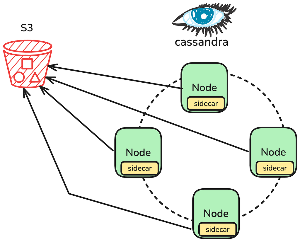
Image 1: Cassandra Cluster Backups to S3

Casspactor: The Engine We Outgrew

Casspactor processed roughly 1,200 data movements per day, transferring approximately 3 PB of data from Apache Cassandra into Apache Iceberg tables. It served some of the most critical workloads at Netflix. For years, it worked. Then, two compounding challenges made it clear we needed a fundamentally different architecture.

Fragile Metadata Dependencies

Before Casspactor could move a single record, it needed to answer a deceptively simple question: which backup exists, is it complete, and what does it contain?

Casspactor assembled this answer from multiple independent systems:
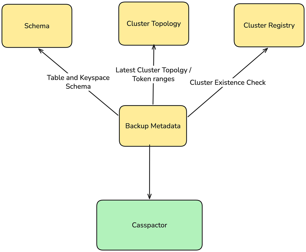
Image 2: Casspactor’s Composite View of a Backup

Each system had its own failure modes, update cadences, and accuracy guarantees. Casspactor’s view of the world was a composite, and composites diverge from reality.

Metadata fell out of sync with actual backups, causing Casspactor to read stale or incorrect data silently. Routine maintenance on the Cassandra Clusters triggered uncoordinated snapshots, and because Casspactor required all nodes in a region to snapshot at the same clock second, a single node replacement could break data movement for an entire region.

The fix was hiding in plain sight. The answer to “which backup exists and is it complete?” already lived in the backup storage layer (Amazon S3) itself. By reading metadata directly from the backup files, we could replace the entire dependency chain with a single source of truth.

Every Connector Inherited Casspactor’s Limitations

Cassandra at Netflix does not just store raw tables. It backs higher level data abstractions, such as Key Value, Time Series, and others, each with its own data model, access patterns, and semantics. When any of these abstractions needed to move data to Iceberg, they all funneled through Casspactor.

Every abstraction inherited Casspactor’s constraints:

  • Skewed partition failures: Casspactor could not handle tables with large partitions, a common pattern in Key Value and Time Series workloads. Jobs crashed with out-of-memory errors on some of Netflix’s largest datasets.
  • No data model awareness: Casspactor moved raw Cassandra tables as is. Connectors for Key Value and other abstractions had to bolt on post processing to reconstruct their data models from the raw output — extra cost, extra complexity, and an extra surface for failures.
  • Intermediate table bloat: Casspactor wrote to an intermediate Iceberg table before producing the final output. The Key Value connector added another intermediate table and a snapshots table. Connectors for abstractions on top of Key Value added even more. This compounded into significant storage cost overhead.
  • Inability to Time Travel: by relying on multiple services to compose a backup unit, Casspactor was unable to restore prior backups in the event of cluster Topology or Keyspace schema changes.
  • Monolithic design: Casspactor was built as a single connector, not as an engine. There was no way to build a family of purpose built connectors on a shared foundation.

We needed something fundamentally different: an engine that reads directly from backups in S3, produces standard Spark DataFrames, and lets each data abstraction build its own connector with full awareness of its data model. One foundation, many connectors.

The New Stack: A Layered Architecture

The new architecture, built upon the foundation of Apache Cassandra Analytics and the in-house Move Data framework, represents a fundamental shift toward a layered, purpose-built stack designed for reuse and maintainability. This new engine was conceived with clear separation of concerns, moving away from Casspactor’s monolithic design. The architecture is intentionally layered with the foundation being a core S3 reading capability: the Cassandra Analytics Wrapper, which is built on top of the Open Source Cassandra Analytics with Netflix’s internal backup representation and an S3 Client.

This layer handles the raw data retrieval from backups, translating it into standard Spark DataFrames. Sitting atop this foundation is a “Connector Factory” model, via both Java UDFs and transforms which allows individual data abstractions (Key Value, Time Series, others) to build highly optimized, data model aware connectors that process the generic Spark DataFrames, avoiding the need for complex, expensive, and failure-prone post-processing steps. This layered approach ensures that improvements to the core reading engine benefit all connectors, while the connectors themselves are focused solely on data transformation.
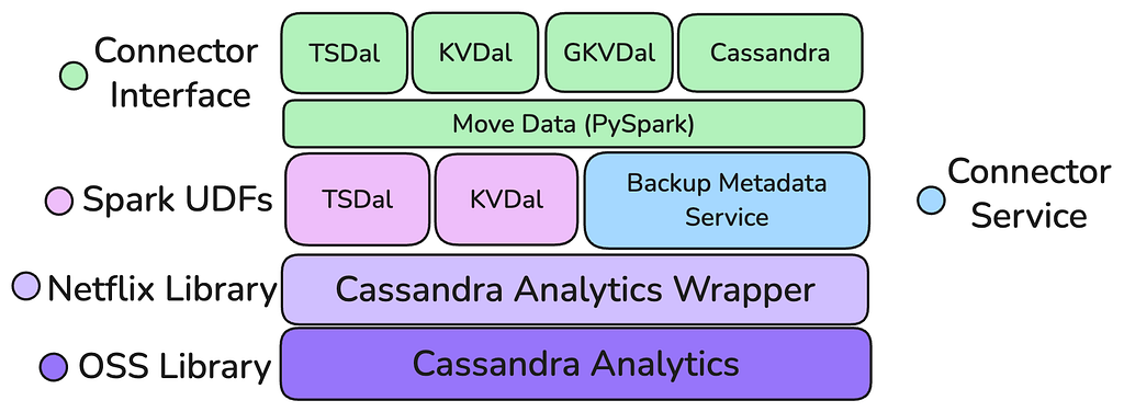
Image 3: The new Connector layered stack
  • Handles Skewed Partitions: By moving the mutation compaction and processing to the Executor level within Spark, the new engine can efficiently handle tables with highly skewed or wide partitions, a major pain point for Casspactor. Crucially, this processing occurs without excessive data shuffling, preventing out-of-memory errors and enabling reliable movement of Netflix’s largest datasets.
  • Operates at Spark DataFrames (No Intermediary Tables): The new architecture directly generates standard Spark DataFrames from the Cassandra backups. This eliminates the need for Casspactor’s costly, multi-stage intermediate Iceberg tables, which led to storage bloat and operational complexity. This native DataFrame operation enables the “Connector Factory” by providing a universal, easily consumable interface for building diverse, model specific connectors.
  • Jobs Auto Size: The engine integrates intelligent auto-sizing capabilities, allowing jobs to dynamically adjust resource consumption based on the source table’s characteristics. This removes the burden of manual tuning from engineering teams, ensuring optimal performance and cost efficiency without sacrificing reliability.
  • Reduced Dependencies: By reading metadata directly from the backup files stored in S3, the new stack removes the fragile, multi-service dependency chain that plagued Casspactor. S3 becomes the single, authoritative source of truth for backup existence and completeness, vastly improving data movement reliability and consistency.
  • Time Travel: A critical feature of the new stack is the ability to process the schema, cluster topology, and data as a cohesive unit at a specific point in time. This capability provides robust time travel functionality, essential for auditing, debugging, disaster recovery and reproducing past data states.
  • Performance: Collectively, these architectural improvements, including native DataFrame processing, optimized partition handling, and streamlined metadata retrieval have resulted in notable performance gains, reducing overall data movement execution runtime and cost compared to the legacy Casspactor system.
  • Cost: by eliminating intermediary Iceberg tables and efficient SSTable compaction on Executors, the new stack needs a significantly smaller storage and compute footprint leading to significant cost savings in the order of USD millions.

The Journey Towards a Safe Migration

The successful validation of the new stack was the critical first step, but it only marked the beginning of the most challenging phase: the migration. Large scale data migrations are inherently complex, high-risk undertakings that can be time consuming and often result in customer frustration and service disruption. To navigate the high stakes of decommissioning a mission-critical system like Casspactor and seamlessly replacing it, we needed a strategy that prioritized reliability and transparency above all else.

The migration was fundamentally enabled by a Like-for-Like strategy, which served as the cornerstone of our Platform Engineering philosophy, abstracting complexity. The core tenet was to maintain absolute consistency across the user-facing interface, the output contract, and the final data artifact. This meant ensuring that the data movement parameters defined via the Data Bridge abstraction remained unchanged, and, critically, the schema, metadata, and data within the destination Iceberg tables were identical to the legacy output. By preserving these external contracts, we eliminated the need for complex, time-consuming coordination with dozens of internal teams who relied on these data pipelines. This approach transformed the migration from a distributed, high-risk, multi-team effort into an internal platform implementation detail, allowing us to achieve a transparent, zero-impact transition and accelerate the retirement of the legacy system without requiring any code changes or validation from downstream users.

To navigate this migration, we developed a strategy anchored by three core pillars that serve as a blueprint for successful, large-scale data migrations:

  1. Validation: Establishing and maintaining absolute confidence in data consistency through rigorous, ongoing validation.
  2. Visibility: Instrumenting every part of the system to provide a clear, real-time understanding of migration progress and system health.
  3. Safety: Ensuring user impact is minimized or eliminated, despite the inevitable system failures, by leveraging abstractions and robust fallbacks.

The next section will provide a detailed exploration of these key pillars.

Pillar 1: Validation

Trust is earned, and in data migration, it is earned one row at a time. The first pillar is the most critical: providing a measurable guarantee to users and partners that the data produced by the new system is an exact, row-by-row replica of the data produced by the old one.

Our foundational tactic was deploying the new Move Data connector in a “shadow” testing that ran in parallel with the production Casspactor jobs. This allowed us to validate the new system with real-world, production workloads without any customer impact.
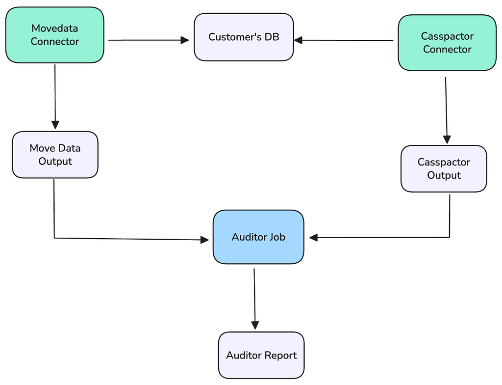
Image 4: Shadow job structure leveraged for data validation
  • Let C be the set of rows in the legacy Casspactor output (Iceberg table).
  • Let M be the set of rows in the new Move Data output (Iceberg table).

The test for trust: prove that C = M. This required continuously checking for two conditions:

  1. Rows in C but not in M (C-M): The new system missed data.
  2. Rows in M but not in C (M-C): The new system introduced phantom or erroneous data.

Any result where the cardinality of these difference sets (the number of differing rows) was greater than zero triggered an immediate, high-priority investigation. The target was 100% similarity.

Uncovering and Resolving Disparities

The shadow mode quickly became a powerful forensic tool, exposing “unknown unknowns”, subtle discrepancies that were not bugs in the new system but rather differences in behavior between the new and old systems. Resolving these was the core work of building trust. For each problem we initiated an investigation log where we captured the details, logs, queries that allowed us to diagnose. Based on the assessment the issues were categorized so that similar differences on other datasets were later resolved affecting many of the shadow pipelines.

Maintaining an investigation log was critical to organize the outstanding issues and effectively communicate to stakeholders the progress and confidence of the new connector so that we effectively measure the appropriate level of “confidence” to initiate the migration.

We observed differences in how connectors leverage reference timestamps for Time-to-Live, Consistency Levels, backup selection, and various internal business logic. This continuous, data-driven cycle of discovery and resolution was the mechanism by which we built confidence in the new architecture.

Pillar 2: Visibility

Trust is built in the background, but an active migration requires real-time insight: Visibility. The second pillar involves instrumenting the system to provide an unambiguous, clear understanding of operational health and migration progress.

We extended our instrumentation to the overall migration workflow and its dependencies:

  • Dashboards: We created centralized dashboards to track migration status, visualizing the total number of data movements migrated versus those remaining. The dashboards tracked execution status, average runtime, and cost comparisons between the two connectors.
  • Dependency Tracking: Since the new system relied on a new set of APIs to fetch backup metadata, we implemented detailed metrics for failures to keep track of the APIs or dependencies failed.
  • Alerting: Proactive alerts were set up for job failures (Move Data or Casspactor), failures on Move Data that triggered a fallback to Casspactor or any data discrepancy being detected.

This comprehensive instrumentation allowed the team to be proactive, fix issues as they emerged during the migration, and gain the necessary confidence to accelerate the migration timeline.

Pillar 3: Safety

Even with perfect data correctness and enhanced visibility, the third pillar, Safety is required for a zero-impact migration. The challenge is ensuring that when a system inevitably fails, the user experience is uninterrupted. Our strategy centered on decoupling the user’s workflow from the underlying connector implementation.

Leveraging Abstraction: The Decider Pattern

To achieve a transparent swap, we leveraged the Maestro workflow orchestration platform to implement the Decider pattern:

  1. Data Movement Abstraction: From a user’s perspective, their Data Movement job definition remained the same.
  2. The Decider Step: Internally the workflow responsible to execute the job was modified to include a Decider step. This step took the data movement parameters (source cluster, table name, destination) and invoked a control plane: Connector Controller.
  3. Connector Controller as the Registry: The control plane served as the dynamic registry. Based on the migration cohort and the data movement attributes, it determined and reported the appropriate connector to use either Casspactor (legacy) or Move Data (new).

This abstraction gave our team complete control. We could upgrade or rollback any connector for any data movement instantly by simply updating a configuration in the controller, with zero modification required to the thousands of downstream customer workflows. Crucially, this abstraction guaranteed the critical safety net: a conditional step in the Maestro workflow logic ensured that if the Move Data step fails, it would immediately execute the Casspactor step.

This pattern would increase the chances that the user’s data movement completes successfully, even if the new connector encountered a bug or transient failure during the initial rollout phases. User impact was completely eliminated; they might see a slightly longer runtime in the event of a failure and fallback, but they would never see a migration failure or suffer from stale data.
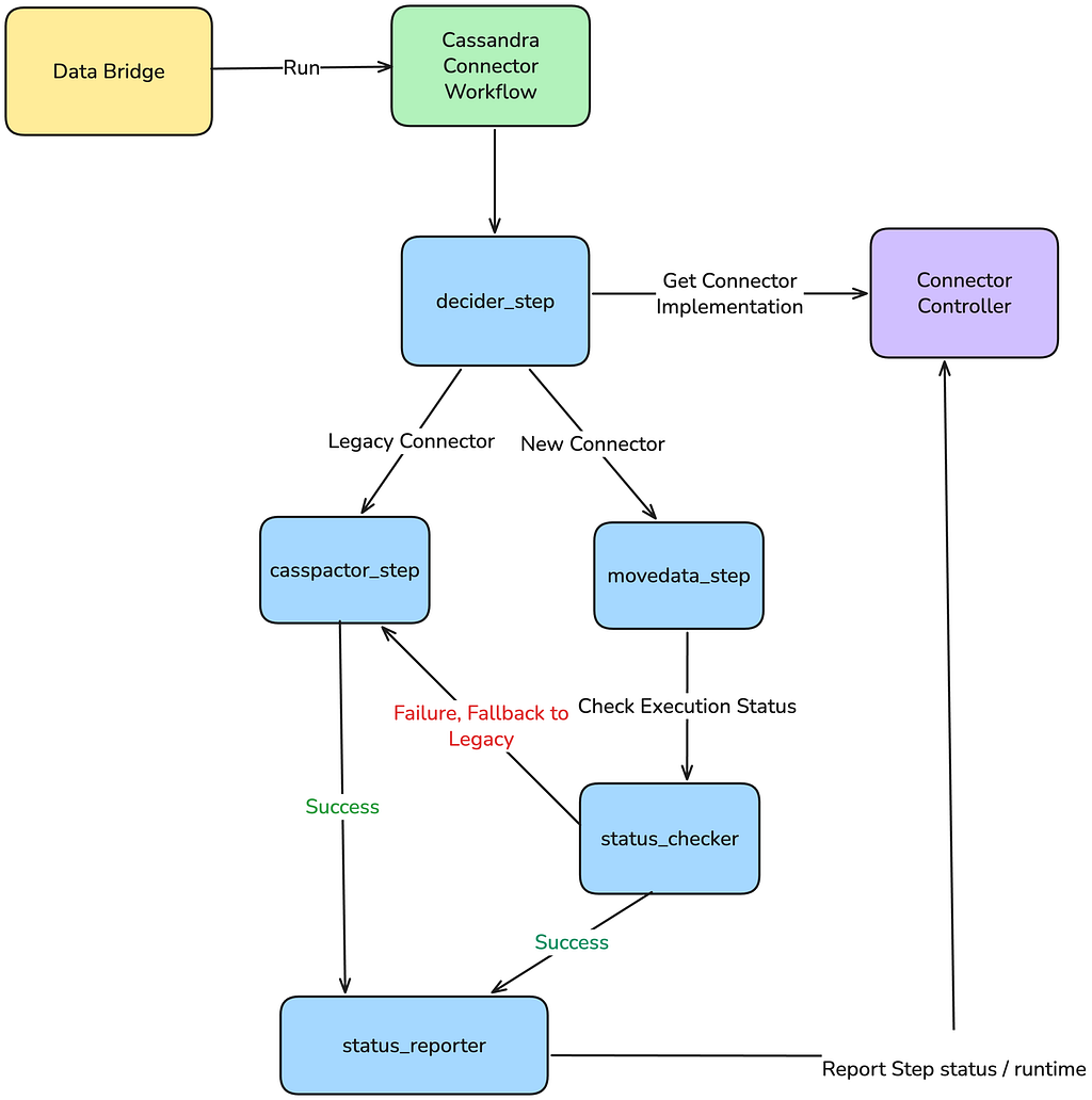
Image 5: The Decider Pattern Implementation via Maestro

Beyond the workflow, the new system architecture itself was inherently more resilient. By building the new data movement connector on Cassandra Analytics and reading backups directly from S3, we removed fragile dependencies on deprecated internal services.

Conclusion

The migration from Casspactor to the new, layered architecture built on Cassandra Analytics and the Move Data connector was more than a typical “tech debt” project; it was a fundamental shift in our approach to data movement reliability and scalability at Netflix.

The legacy system, while serving us well for years, was ultimately constrained by monolithic design, fragile metadata dependencies, and an inability to handle the complexity of modern data abstractions. The new stack resolves these issues by delivering a robust, cost-efficient, and inherently more resilient solution that reads directly from S3, handles wide partitions gracefully, and eliminates costly intermediate tables.

Our blueprint for the migration, anchored by the three pillars of Validation, Visibility, and Safety, ensured a transparent and high-confidence transition. Through rigorous shadow testing and a data-driven audit framework, we achieved the desired data consistency. Enhanced dashboards and alerting provided the real-time operational insight necessary to manage risk. Most critically, the implementation of the Decider pattern within our workflow abstraction minimized the impact for all downstream users.

This successful migration validates a core philosophy: by abstracting complexity at the platform level, we can perform large system migrations without burdening our product engineering partners. The new foundation is now ready to support the next generation of Netflix’s data abstractions.

Looking ahead

This foundational work on the Cassandra Data Movement stack has done more than just replace a legacy system: it has become an accelerator for innovation across the entire Data Movement organization. By providing a reliable, performant engine that standardizes data retrieval into Spark DataFrames, we’ve enabled the rapid development of new, highly optimized connectors. This new “Connector Factory” approach has already delivered a dedicated Key-Value to Iceberg and Time Series connectors, both of which are fully aware of their respective data models, eliminating costly post-processing. This architecture is also paving the way for ambitious new initiatives, including the development of a solution for bulk loading data into Cassandra itself, effectively completing the data movement cycle, and enabling safer fleetwide connector rollout with canaries inspired by the Decider Pattern.

We are incredibly grateful for the extensive collaboration among the Data Movement, Data Bridge, Online Data Stores, Membership, Billing, Subscriber and Ads platform teams at Netflix; this work simply couldn’t have been accomplished without their partnership!


The Evolution of Cassandra Data Movement at Netflix was originally published in Netflix TechBlog on Medium, where people are continuing the conversation by highlighting and responding to this story.
Dynamically Splitting Wide Partitions in Cassandra for Time Series Workloads

Post Syndicated from Netflix Technology Blog original https://netflixtechblog.com/dynamically-splitting-wide-partitions-in-cassandra-for-time-series-workloads-0eded064f456

By Rajiv Shringi, Kaidan Fullerton, Oleksii Tkachuk and Kartik Sathyanarayanan

Introduction

Netflix’s TimeSeries Abstraction is a scalable system for ingesting and querying petabytes of temporal event data with millisecond latency. We use Apache Cassandra 4.x as the underlying storage for these main reasons:

  • Throughput, latency, and cost: Cassandra can handle millions of low‑latency reads and writes in a cost-effective manner.
  • Operational maturity: Our data platform team has deep operational expertise running large Cassandra clusters in production.

However, using Cassandra at this scale introduces trade‑offs for TimeSeries workloads. A key challenge is wide partitions, as TimeSeries dataset partitions can grow quite large with events accumulating over time.

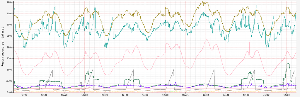
This problem is further compounded by the fact that TimeSeries servers routinely deal with a very high read throughput:

Reads/second for different datasets

This post walks through our journey to reduce the impact of wide partitions in our TimeSeries datasets, the solutions we built, and the lessons we learned.

Impact of Wide Partitions

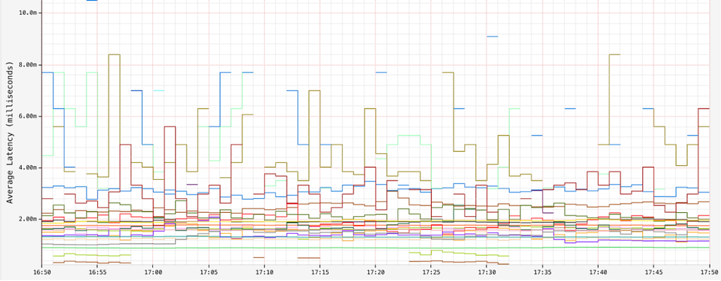
For most of our datasets, we observe an average read latency in the order of single-digit milliseconds:

Ideal Latency for Reads (ms)

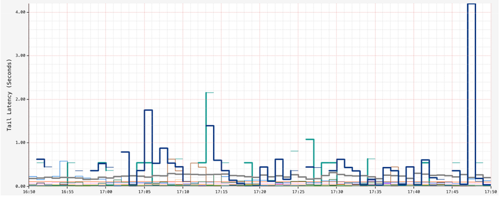
However, in some datasets, as partitions grow too wide, we observe high read latencies in the order of seconds, especially towards the tail end:

High Tail Latency for Reads (seconds)

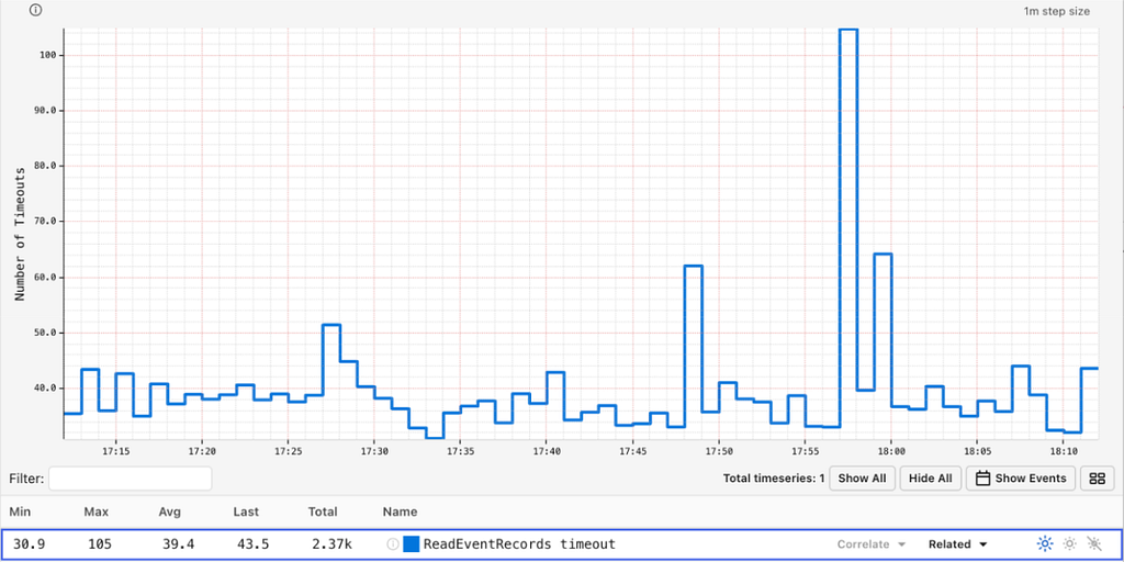
This can result in timeouts:

Read timeouts / second

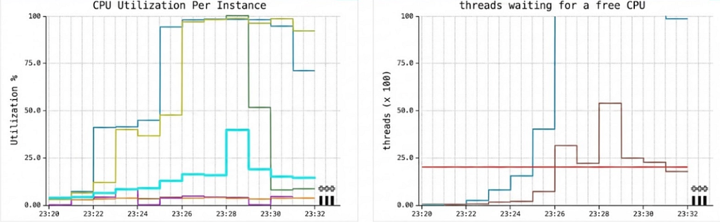
In extreme cases, if most of the reads target wide partitions, we can see Garbage Collection pauses, high CPU utilization and thread queueing.

High CPU utilization and thread-queueing in Cassandra clusters

Scaling up the underlying Cassandra cluster is always an option, but we need smarter alternatives than just throwing more money at the problem.

TimeSeries Partitioning Strategy

The TimeSeries Abstraction was designed to solve the problem of wide partitions by dividing the data into discrete time chunks. For more in-depth information, refer to our previous blog.

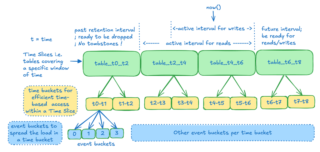
To summarize, here is an illustration of how TimeSeries partitioning strategy helps us break up wide partitions into manageable chunks.

Time Series partitioning breaking up a dataset into Time slices, time buckets and event buckets

This strategy further allows us to efficiently query and drop data based on time, without having to deal with tombstones.

Picking the Partitioning Strategy

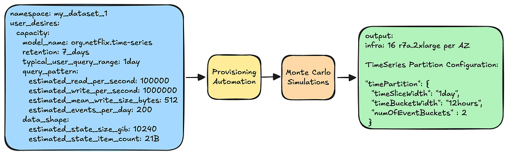
When a namespace (a.k.a. dataset) is created, users must specify their anticipated workload characteristics. This specification is then fed into our provisioning pipeline. The pipeline processes these inputs, runs Monte Carlo simulations, and produces an optimal infrastructure and partition configuration.

Provisioning picks optimal infra and configuration based on user inputs

You can learn more about our methodology of capacity planning in this insightful AWS re:Invent talk given by one of our stunning colleagues.

The Problem with the Current Approach

Although this method of provisioning is effective in many situations, it proves insufficient for TimeSeries workloads under these conditions:

  • Workload is unknown or inaccurately estimated: Early on in a project, users can lack a reliable picture of production traffic or simply misestimate key parameters.
  • Workload evolves over time: Traffic patterns, client behavior, and product requirements change. A “good” partitioning strategy on day one can become inefficient months later.
  • Data outliers exist: Not all TimeSeries IDs behave the same. A small percentage of IDs can receive a vastly higher volume of events than the rest.

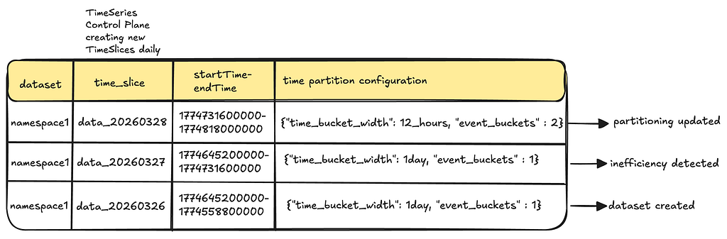
Fortunately, our design with discrete Time Slices gives us a natural escape hatch for the first two scenarios; each new Time Slice can use a different partitioning strategy.

Each Time Slice can have a unique partition strategy

However, manually adjusting these configurations in a fleet that has thousands of TimeSeries datasets is not sustainable. We need automation.

Solution 1: Time Slice Re-Partitioning

Cassandra exposes useful introspection APIs for understanding data usage and access patterns. For example, nodetool tablehistograms provide percentile distributions for partition sizes in a table. Using these tools, we can detect cases of both over and under partitioning.

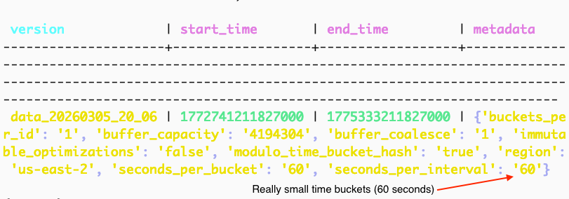
Below is an example of over‑partitioning, where the TimeSeries provisioning pipeline selected very small time_bucket intervals based on user provided inputs:

Provisioning selected 60s time buckets based on user inputs

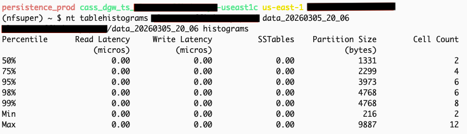
causing partitions to have less than 10 KB of data, leading to high read amplification and thread queueing:

Histogram of the given Cassandra table showing partition size percentiles

In order to tune partition strategies efficiently, we added a background worker, which monitors partition histograms of Time Slices attached to a given application, and exposes it via a Cassandra virtual table:

Histograms exposed through a Cassandra Virtual table

It then computes an adjustment factor when it detects partition sizes not meeting a configured density. This configured density is often set between 2 MiB to 10 MiB depending on the workload.

DynamicTimeSliceConfigWorker: 
namespace: my_dataset_1
Observed: TimeSlices have p99 partitions below configured target of 10MB.
Proposed: time_bucket interval: 60s -> 604800s

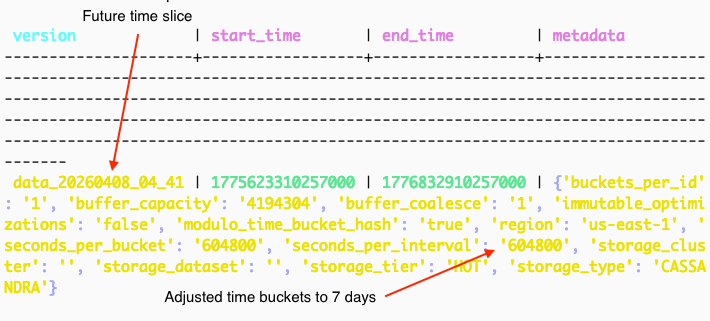
The worker can then update future Time Slices with the new partition strategy:

Partitioning adjusted for future Time Slice(s)

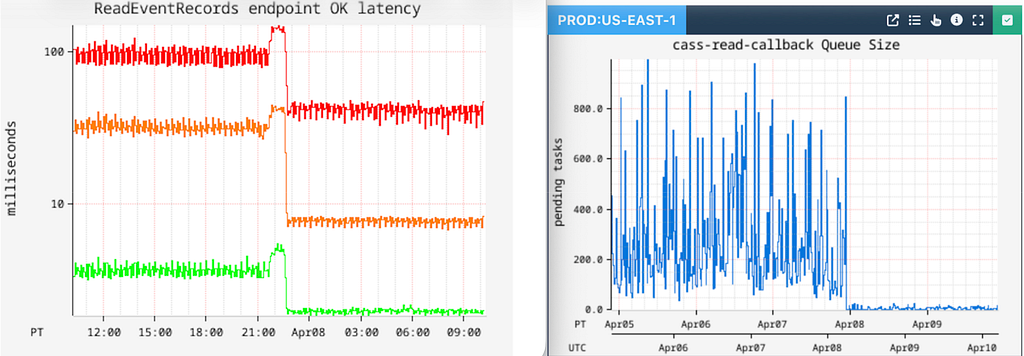
This strategy has yielded real results in reducing our read latencies, as well as reducing the number of timeouts caused by thread queueing.

Reduction in tail latency and thread queueing for

However, this strategy only works if most of the data exhibits such behavior that warrants re-partitioning of the entire table. It does not work in cases where only a percentage of IDs within the table are wide.

We have a couple of options here:

  • Do Nothing: This is sometimes the right approach if there is no observed impact to the application’s top-level metrics.
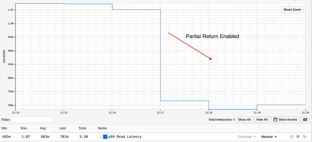
  • Partial Returns: We implemented a ‘Partial Return’ feature, which aborts an inflight request if it has breached a configured latency SLO, while returning whatever data it has collected up until that point. This is a great option for clients who care more about latency than fetching all the data.
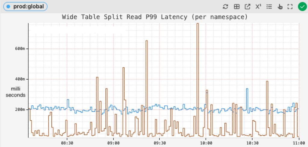
Tail latency drops around the SLO cutoff as Partial Returns are enabled
  • Block IDs: This is an extreme step but worth mentioning, because we do deal with bad data that occasionally seeps into the system e.g. test or spam IDs that can make the system unstable.
dgwts.config.<dataset>.block.Ids: "<tsid-1>, <tsid-2>, <tsid-3>"

Ultimately, we encounter scenarios where valid and important TimeSeries IDs accumulate a high enough volume of events, with callers needing to process all the related data. Simply tolerating elevated latencies or timeouts when querying these IDs is not a desirable outcome.

This is where dynamic partitioning comes into play.

Solution 2: Dynamic Partitioning per ID

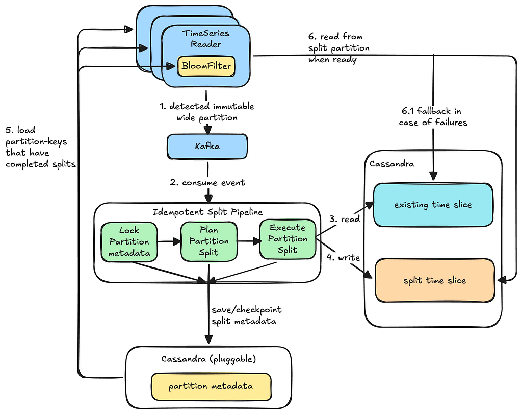
Dynamic partitioning is an asynchronous pipeline that auto-detects and splits wide partitions on a TimeSeries ID level rather than at the table level.

It has three main stages:

  • Detection: Detects wide partitions for a given TimeSeries ID during the read path.
  • Planning & Splitting: Plans and executes splits of those partitions into optimal sizes asynchronously.
  • Serving Reads: Re-routes the read queries transparently to read data from the split partitions when ready.

This is how it works at a high level; we will dive into details after:

Dynamic Wide Partition Split Async Pipeline

Here are the different stages of the pipeline:

Detection

Every TimeSeries read operation tracks how many bytes are read for a given partition. If the bytes read exceed a configured threshold, the server emits a detection event to Kafka:

{
"time_slice": "data_20260328", // the Cassandra table this event was detected in
"time_series_id": "profileId:123", // the ID detected as wide
"time_bucket": 7, // the existing time_bucket partition
"event_bucket": 2, // the existing event_bucket partition
"immutable": true, // TimeSeries servers can compute if this partition is no longer receiving writes
"version": "0" // reserved for future use e.g. invalidate if partition is no longer immutable
}

Our decision to detect wide partitions on reads, as opposed to writes, is based on our observation that the majority of the data in the wild doesn’t need this treatment. The slight downside is that some reads on these large partitions may suffer sub-optimal performance for a very short duration (typically seconds) until this process catches up.

Immutability

Although splitting mutable partitions is possible, it is inherently more complex. As a first step towards solving this problem, we chose to reduce the surface area of this change by focusing on immutable partitions, while still meaningfully reducing caller timeouts.

Planning

Detection may occur based on a partial read, so the planner must still read the entire partition once to compute an accurate split plan. The checkpointing becomes crucial here. For planning reads that fail to process the entire partition, the process can always continue from the last saved checkpoint.

Checkpointing

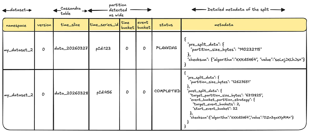
The wide_row metadata table serves as the backbone for state transitions and checkpointing of partition splits. It also stores information that is used later by TimeSeries servers to properly route Read queries.

wide_row metadata for storing split states and checkpoints

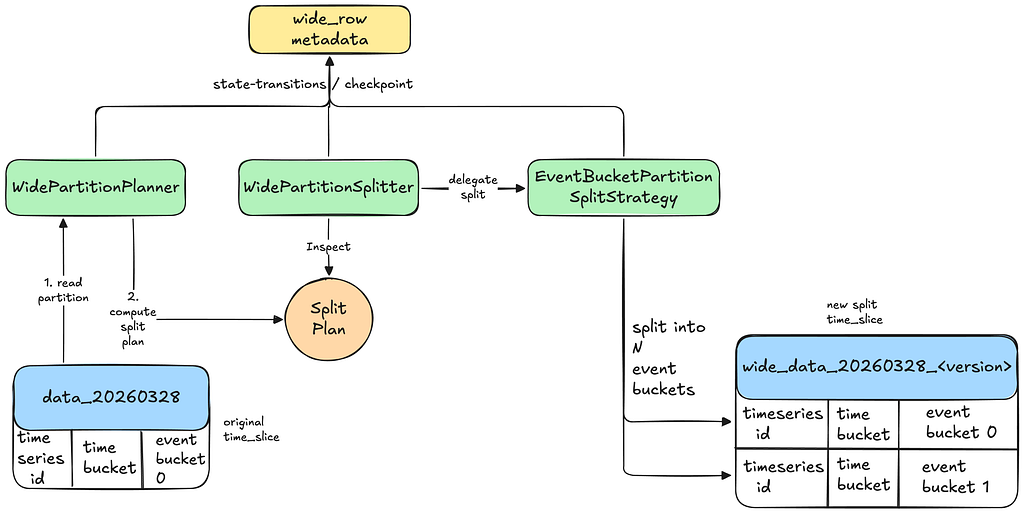
Splitting

The Planner delegates the splitting of data to an appropriate split-strategy. For example, if EventBucketPartitionSplitStrategy is selected, we split the partition by assigning more event buckets to the same time bucket. If the partition is ultra-wide, we cap the number of event buckets we split into, in order to control the resultant read amplification. Spreading into multiple partitions in such cases is still beneficial in order to spread the read workload to multiple Cassandra replicas.

Split by assigning more event buckets for a given time bucket

Validating Splits

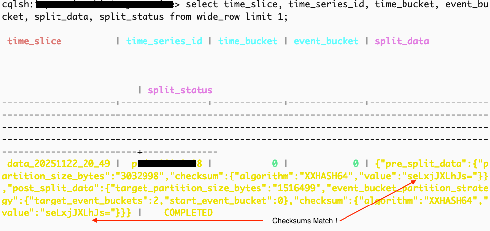
The Planner stores a pre-split checksum of a given partition during the planning phase, while the Splitter computes and stores the post-split checksum. The split status is marked as completed only if the two checksums match.

Ensure checksums match pre- and post-split before marking a split as COMPLETED

Tracking Splits

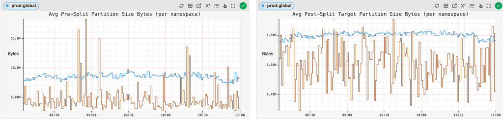
The pre- and post-split partition sizes across different datasets are tracked to see how effectively the partition splits are being planned and executed:

Track pre- and post-split partition sizes to ensure we are splitting optimally

Serving Reads

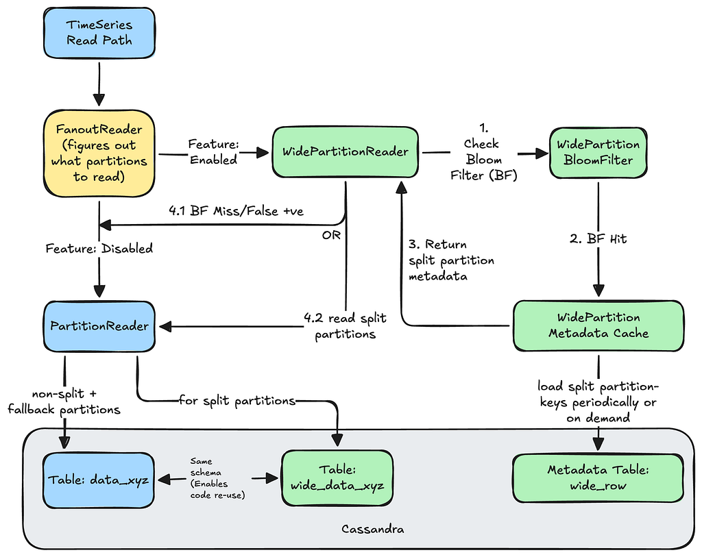
The TimeSeries servers load the partition-keys of completed splits periodically into in-memory Bloom filters. Every read operation checks the Bloom filter to see whether a query can be diverted to the split partitions.

Here is what the Read path looks like:

Read path for diverting reads to existing or split partitions

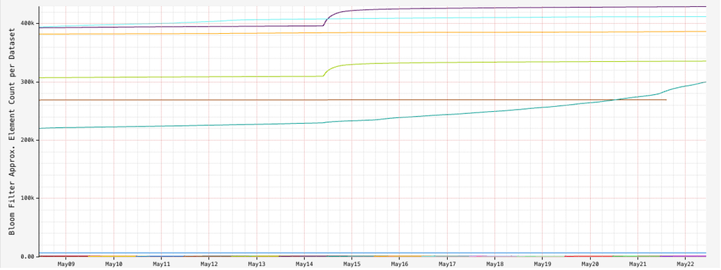
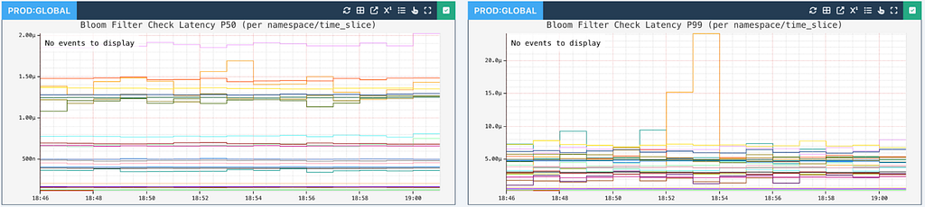
The size of the Bloom filters is monitored to ensure we have enough memory per server. Due to the compactness of partition keys, and ratio of wide partitions in a given dataset, the filters fit comfortably in each server instance.

Bloom filter approximate element count per namespace and time slice

The Bloom filter latency to check whether a given partition key is wide for every read request is typically in single-digit microseconds or better, making this diversion practically invisible to the callers.

Latency for checking Bloom filters is extremely small for callers to notice the diversion

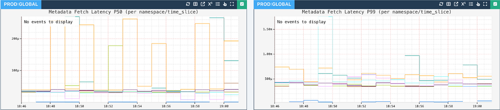
For the cases that do end up with a Bloom filter hit, the TimeSeries servers lookup the wide_row metadata to see how to read a specific wide partition:

{
"pre_split_data": {
"time_slice": "data_20260328",
"time_series_id": "6313825", → What to read
"time_bucket": 0,
"event_bucket": 2

},
"post_split_data": {
"time_slice": "wide_data_20260328_0", → Where to read it from
"event_bucket_partition_strategy": { → Strategy to delegate to for reading
"target_event_buckets": 2,
"start_event_bucket": 32 → How should the strategy read it
}

}

This metadata read is backed by a read-through cache, making it quite performant:

Metadata fetch latency is quite low to affect read operations

Finally, the reads for the split partitions are delegated to our existing PartitionReader. Having the same schema for the split table allows us to reuse code and minimize changes.

Fallbacks

The existing wide partition from the original time slice is never deleted. This helps us in creating safe fallbacks in many different scenarios of partial failures and eventual consistency. The slightly larger storage space we use as a result is worth the operational safety we gain.

Building Additional Confidence

Serving incorrect reads would be disastrous. To establish trust beyond checksums, we leveraged additional mechanisms such as:

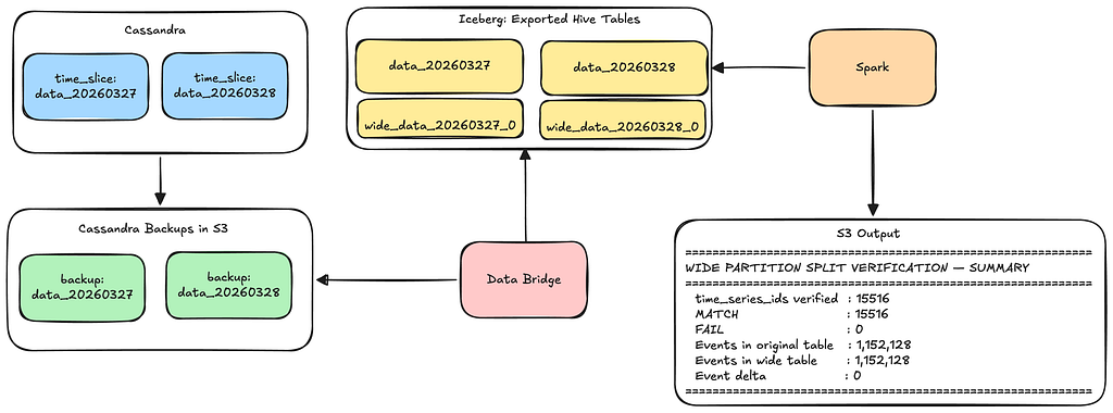
  • Using our existing Data Bridge pipelines to verify splits offline:
Spark job to ensure that the split data is an exact match to the original data
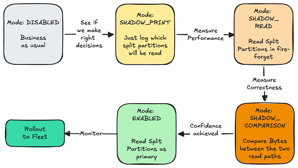
  • Implementing a phased rollout strategy to safely advance through stages as our confidence in the system grew:
Advance through Read modes once previous mode passes checks

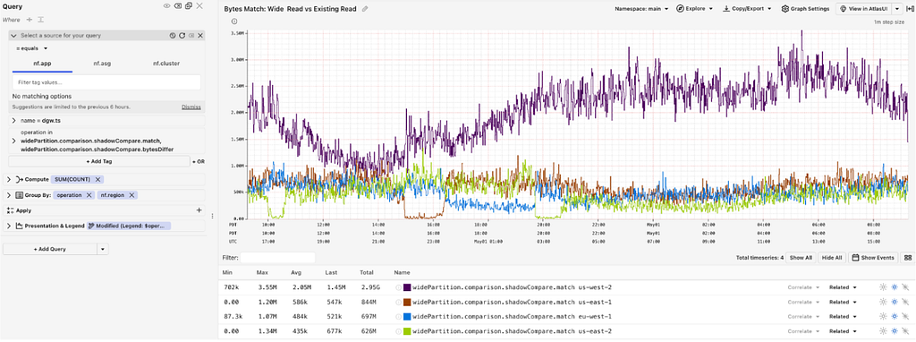
A critical part of this phased rollout was the Comparison phase, which compared bytes served by old read path and the new read path while in shadow mode:

A chart of bytes match vs bytes differ in a given shadow period

Results

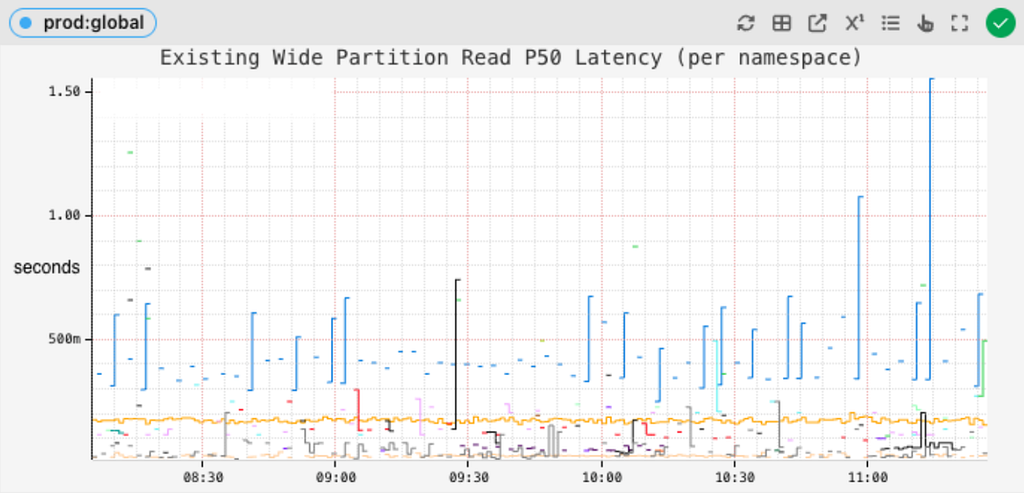
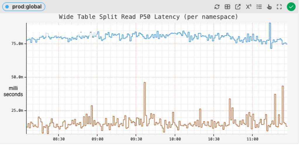
As a result of these dynamic splits, we see a huge improvement in the average read latency of most wide partitions, bringing it down from seconds:

Existing average latency for reading wide partitions

to low double-digit milliseconds!

Average latency for reading dynamically split partitions

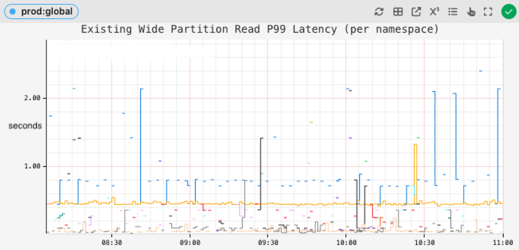
Tail latencies of reading wide partitions dropped from several seconds:

Existing tail latency for reading wide partitions

to around 200 ms or better:

Tail latency for reading dynamically split partitions

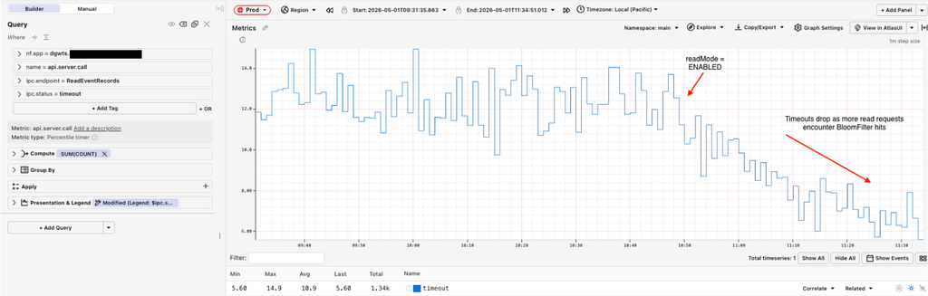
resulting in a drop in read timeouts:

Further, for extreme wide rows, where a dataset would face constant timeouts and unavailability blips, the service was able to paginate and query 500MB+ partitions while remaining available:

grpc … com.netflix.dgw.ts.TimeSeriesService/SearchEventRecords -d
'{"namespace": "...",
"search_query": {...},
"time_interval": {
"start": "2026–05–11T23:42:51.484398Z",
"end": "2026–05–12T00:13:50.694205Z"
},
"pageSize" : 1000,
}'
# Response:
{
"next_page_token" : ….,
"records": [
{

}
],
"response_context": [{
"namespace": "...",

# Trades elevated latency for being available
"time_taken": "41.072410142s"
}
]
}

Conclusion

There is more work planned around this feature, like splitting mutable wide partitions, or re-processing previously failed splits, but this has been a successful start in improving service performance and reducing our support burden.

Further, we would like to highlight some key lessons that we learned at different points in this journey.

  • Reducing Surface Area: As a first step, explore simpler solutions that can still deliver meaningful impact. Also, reducing the surface area of a complex change and deploying incrementally pays off operationally.
  • Building Confidence: Invest time and resources to build confidence in new features, especially when justified by the feature complexity, deployment blast radius, and/or potential impact.

Acknowledgements: Special thanks to our stunning colleagues who further contributed to this feature’s success: Tom DeVoe, Chris Lohfink, Sumanth Pasupuleti and Joey Lynch.


Dynamically Splitting Wide Partitions in Cassandra for Time Series Workloads was originally published in Netflix TechBlog on Medium, where people are continuing the conversation by highlighting and responding to this story.
Data Reprocessing Pipeline in Asset Management Platform @Netflix

Post Syndicated from Netflix Technology Blog original https://netflixtechblog.com/data-reprocessing-pipeline-in-asset-management-platform-netflix-46fe225c35c9

By Meenakshi Jindal

Overview

At Netflix, we built the asset management platform (AMP) as a centralized service to organize, store and discover the digital media assets created during the movie production. Studio applications use this service to store their media assets, which then goes through an asset cycle of schema validation, versioning, access control, sharing, triggering configured workflows like inspection, proxy generation etc. This platform has evolved from supporting studio applications to data science applications, machine-learning applications to discover the assets metadata, and build various data facts.

During this evolution, quite often we receive requests to update the existing assets metadata or add new metadata for the new features added. This pattern grows over time when we need to access and update the existing assets metadata. Hence we built the data pipeline that can be used to extract the existing assets metadata and process it specifically to each new use case. This framework allowed us to evolve and adapt the application to any unpredictable inevitable changes requested by our platform clients without any downtime. Production assets operations are performed in parallel with older data reprocessing without any service downtime. Some of the common supported data reprocessing use cases are listed below.

Production Use Cases

  • Real-Time APIs (backed by the Cassandra database) for asset metadata access don’t fit analytics use cases by data science or machine learning teams. We build the data pipeline to persist the assets data in the iceberg in parallel with cassandra and elasticsearch DB. But to build the data facts, we need the complete data set in the iceberg and not just the new. Hence the existing assets data was read and copied to the iceberg tables without any production downtime.
  • Asset versioning scheme is evolved to support the major and minor version of assets metadata and relations update. This feature support required a significant update in the data table design (which includes new tables and updating existing table columns). Existing data got updated to be backward compatible without impacting the existing running production traffic.
  • Elasticsearch version upgrade which includes backward incompatible changes, so all the assets data is read from the primary source of truth and reindexed again in the new indices.
  • Data Sharding strategy in elasticsearch is updated to provide low search latency (as described in blog post)
  • Design of new Cassandra reverse indices to support different sets of queries.
  • Automated workflows are configured for media assets (like inspection) and these workflows are required to be triggered for old existing assets too.
  • Assets Schema got evolved that required reindexing all assets data again in ElasticSearch to support search/stats queries on new fields.
  • Bulk deletion of assets related to titles for which license is expired.
  • Updating or Adding metadata to existing assets because of some regressions in client application/within service itself.

Data Reprocessing Pipeline Flow

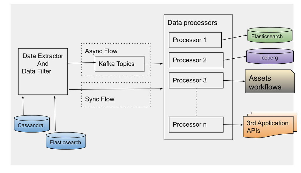
Figure 1. Data Reprocessing Pipeline Flow

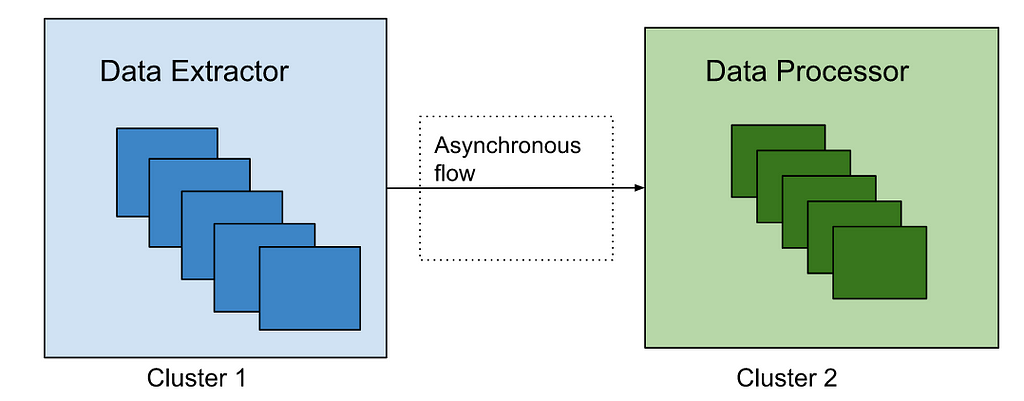
Data Extractor

Cassandra is the primary data store of the asset management service. With SQL datastore, it was easy to access the existing data with pagination regardless of the data size. But there is no such concept of pagination with No-SQL datastores like Cassandra. Some features are provided by Cassandra (with newer versions) to support pagination like pagingstate, COPY, but each one of them has some limitations. To avoid dependency on data store limitations, we designed our data tables such that the data can be read with pagination in a performant way.

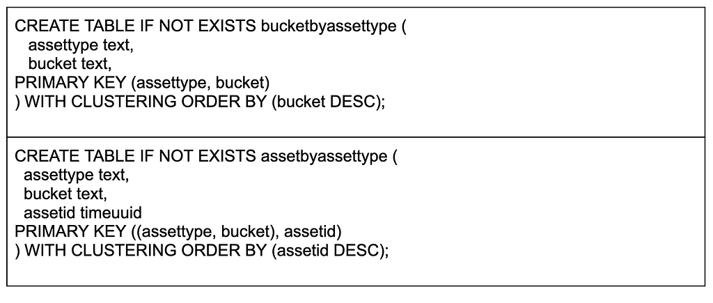
Mainly we read the assets data either by asset schema types or time bucket based on asset creation time. Data sharding completely based on the asset type may have created the wide rows considering some types like VIDEO may have many more assets compared to others like TEXT. Hence, we used the asset types and time buckets based on asset creation date for data sharding across the Cassandra nodes. Following is the example of tables primary and clustering keys defined:

Figure 2. Cassandra Table Design

Based on the asset type, first time buckets are fetched which depends on the creation time of assets. Then using the time buckets and asset types, a list of assets ids in those buckets are fetched. Asset Id is defined as a cassandra Timeuuid data type. We use Timeuuids for AssetId because it can be sorted and then used to support pagination. Any sortable Id can be used as the table primary key to support the pagination. Based on the page size e.g. N, first N rows are fetched from the table. Next page is fetched from the table with limit N and asset id < last asset id fetched.

Figure 3. Cassandra Data Fetch Query

Data layers can be designed based on different business specific entities which can be used to read the data by those buckets. But the primary id of the table should be sortable to support the pagination.

Sometimes we have to reprocess a specific set of assets only based on some field in the payload. We can use Cassandra to read assets based on time or an asset type and then further filter from those assets which satisfy the user’s criteria. Instead we use Elasticsearch to search those assets which are more performant.

After reading the asset ids using one of the ways, an event is created per asset id to be processed synchronously or asynchronously based on the use case. For asynchronous processing, events are sent to Apache Kafka topics to be processed.

Data Processor

Data processor is designed to process the data differently based on the use case. Hence, different processors are defined which can be extended based on the evolving requirements. Data can be processed synchronously or asynchronously.

Synchronous Flow: Depending on the event type, the specific processor can be directly invoked on the filtered data. Generally, this flow is used for small datasets.

Asynchronous Flow: Data processor consumes the data events sent by the data extractor. Apache Kafka topic is configured as a message broker. Depending on the use case, we have to control the number of events processed in a time unit e.g. to reindex all the data in elasticsearch because of template change, it is preferred to re-index the data at certain RPS to avoid any impact on the running production workflow. Async processing has the benefit to control the flow of event processing with Kafka consumers count or with controlling thread pool size on each consumer. Event processing can also be stopped at any time by disabling the consumers in case production flow gets any impact with this parallel data processing. For fast processing of the events, we use different settings of Kafka consumer and Java executor thread pool. We poll records in bulk from Kafka topics, and process them asynchronously with multiple threads. Depending on the processor type, events can be processed at high scale with right settings of consumer poll size and thread pool.

Each of these use cases mentioned above looks different, but they all need the same reprocessing flow to extract the old data to be processed. Many applications design data pipelines for the processing of the new data; but setting up such a data processing pipeline for the existing data supports handling the new features by just implementing a new processor. This pipeline can be thoughtfully triggered anytime with the data filters and data processor type (which defines the actual action to be performed).

Error Handling

Errors are part of software development. But with this framework, it has to be designed more carefully as bulk data reprocessing will be done in parallel with the production traffic. We have set up the different clusters of data extractor and processor from the main Production cluster to process the older assets data to avoid any impact of the assets operations live in production. Such clusters may have different configurations of thread pools to read and write data from database, logging levels and connection configuration with external dependencies.

Figure 4: Processing clusters

Data processors are designed to continue processing the events even in case of some errors for eg. There are some unexpected payloads in old data. In case of any error in the processing of an event, Kafka consumers acknowledge that event is processed and send those events to a different queue after some retries. Otherwise Kafka consumers will continue trying to process the same message again and block the processing of other events in the topic. We reprocess data in the dead letter queue after fixing the root cause of the issue. We collect the failure metrics to be checked and fixed later. We have set up the alerts and continuously monitor the production traffic which can be impacted because of the bulk old data reprocessing. In case any impact is noticed, we should be able to slow down or stop the data reprocessing at any time. With different data processor clusters, this can be easily done by reducing the number of instances processing the events or reducing the cluster to 0 instances in case we need a complete halt.

Best Practices

  • Depending on existing data size and use case, processing may impact the production flow. So identify the optimal event processing limits and accordingly configure the consumer threads.
  • If the data processor is calling any external services, check the processing limits of those services because bulk data processing may create unexpected traffic to those services and cause scalability/availability issues.
  • Backend processing may take time from seconds to minutes. Update the Kafka consumer timeout settings accordingly otherwise different consumer may try to process the same event again after processing timeout.
  • Verify the data processor module with a small data set first, before trigger processing of the complete data set.
  • Collect the success and error processing metrics because sometimes old data may have some edge cases not handled correctly in the processors. We are using the Netflix Atlas framework to collect and monitor such metrics.

Acknowledgements

Burak Bacioglu and other members of the Asset Management platform team have contributed in the design and development of this data reprocessing pipeline.


Data Reprocessing Pipeline in Asset Management Platform @Netflix was originally published in Netflix TechBlog on Medium, where people are continuing the conversation by highlighting and responding to this story.
Exploring Data @ Netflix

Post Syndicated from Netflix Technology Blog original https://netflixtechblog.com/exploring-data-netflix-9d87e20072e3

By Gim Mahasintunan on behalf of Data Platform Engineering.

Supporting a rapidly growing base of engineers of varied backgrounds using different data stores can be challenging in any organization. Netflix’s internal teams strive to provide leverage by investing in easy-to-use tooling that streamlines the user experience and incorporates best practices.

In this blog post, we are thrilled to share that we are open-sourcing one such tool: the Netflix Data Explorer. The Data Explorer gives our engineers fast, safe access to their data stored in Cassandra and Dynomite/Redis data stores.

Netflix Data Explorer on GitHub

History

We began this project several years ago when we were onboarding many new Dynomite customers. Dynomite is a high-speed in-memory database, providing highly available cross datacenter replication while preserving Redis-like semantics. We wanted to lower the barrier for adoption so users didn’t need to know datastore-specific CLI commands, could avoid mistakenly running commands that might negatively impact performance, and allow them to access the clusters they frequented every day.

As the project took off, we saw a similar need for our other datastores. Cassandra, our most significant footprint in the fleet, seemed like a great candidate. Users frequently had questions on how they should set up replication, create tables using an appropriate compaction strategy, and craft CQL queries. We knew we could give our users an elevated experience, and at the same time, eliminate many of the common questions on our support channels.

We’ll explore some of the Data Explorer features, and along the way, we’ll highlight some of the ways we enabled the OSS community while still handling some of the unique Netflix-specific use cases.

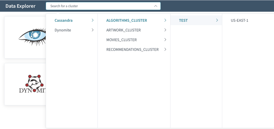
Multi-Cluster Access

By simply directing users to a single web portal for all of their data stores, we can gain a considerable increase in user productivity. Furthermore, in production environments with hundreds of clusters, we can reduce the available data stores to those authorized for access; this can be supported in OSS environments by implementing a Cluster Access Control Provider responsible for fetching ownership information.

Browsing your accessible clusters in different environments and regions

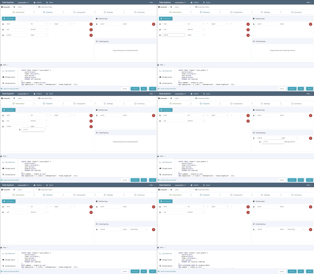
Schema Designer

Writing CREATE TABLE statements can be an intimidating experience for new Cassandra users. So to help lower the intimidation factor, we built a schema designer that lets users drag and drop their way to a new table.

The schema designer allows you to create a new table using any primitive or collection data type, then designate your partition key and clustering columns. It also provides tools to view the storage layout on disk; browse the supported sample queries (to help design efficient point queries); guide you through the process of choosing a compaction strategy, and many other advanced settings.

Dragging and dropping your way to a new Cassandra table

Explore Your Data

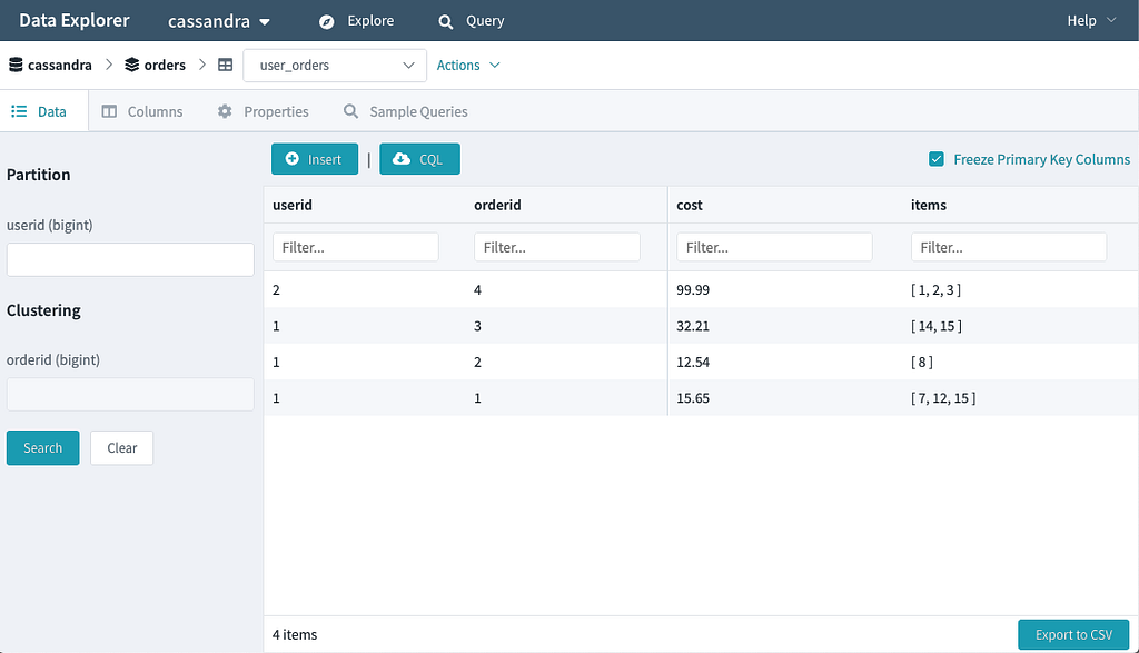
You can quickly execute point queries against your cluster in Explore mode. The Explore mode supports full CRUD of records and allows you to export result sets to CSV or download them as CQL insert statements. The exported CQL can be a handy tool for quickly replicating data from a PROD environment to your TEST environment.

Explore mode gives you quick access to table data

Support for Binary Data

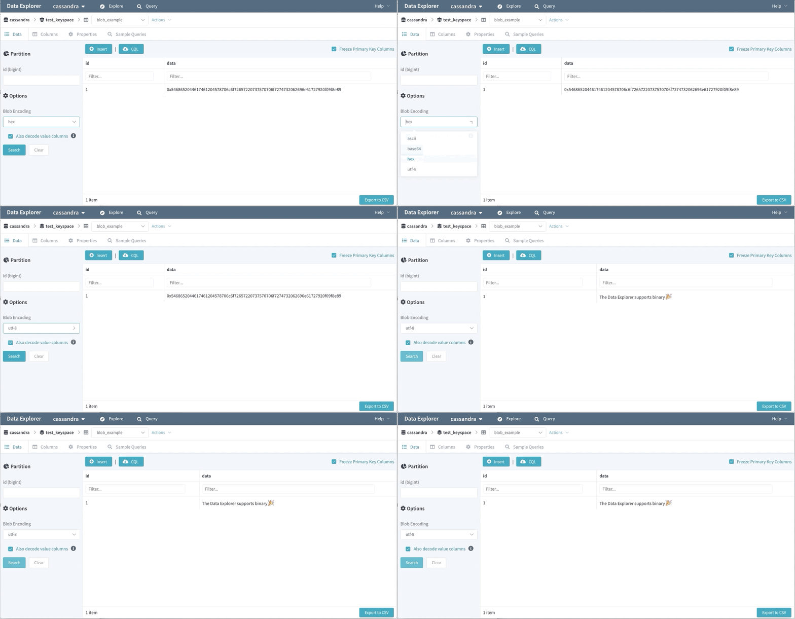
Binary data is another popular feature used by many of our engineers. The Data Explorer won’t fetch binary value data by default (as the persisted data might be sizable). Users can opt-in to retrieve these fields with their choice of encoding.

Choosing how you want to decode blob data

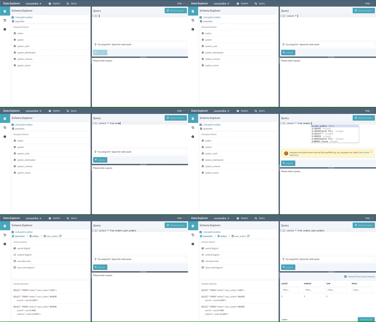
Query IDE

Efficient point queries are available in the Explore mode, but you may have users that still require the flexibility of CQL. Enter the Query mode, which includes a powerful CQL IDE with features like autocomplete and helpful snippets.

Example of free-form Cassandra queries with autocomplete assistance

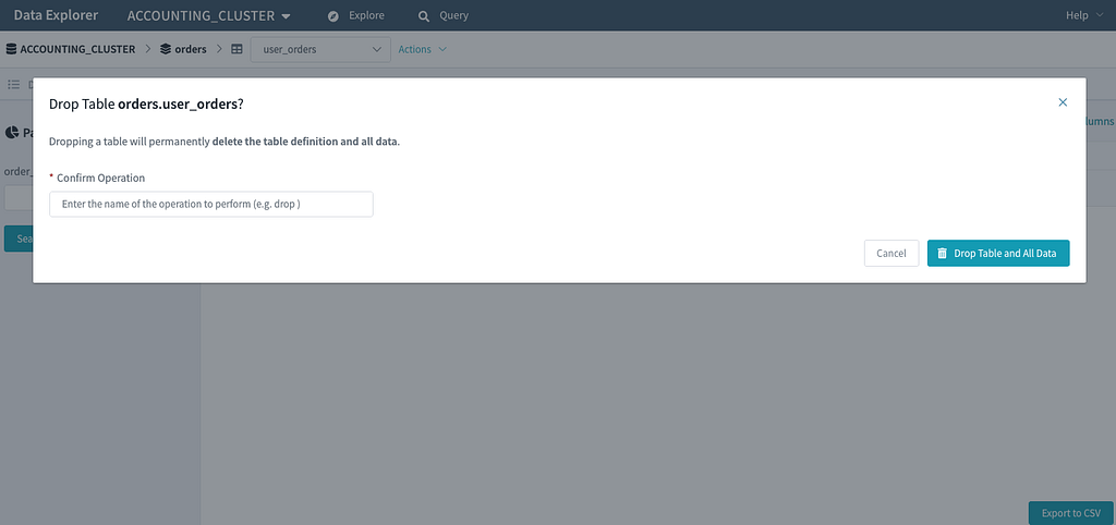
There are also guardrails in place to help prevent users from making mistakes. For instance, we’ll redirect the user to a bespoke workflow for deleting a table if they try to perform a “DROP TABLE…” command ensuring the operation is done safely with additional validation. (See our integration with Metrics later in this article.)

As you submit queries, they will be saved in the Recent Queries view as well — handy when you are trying to remember that WHERE clause you had crafted before the long weekend.

Dynomite and Redis Features

While C* is feature-rich and might have a more extensive install base, we have plenty of good stuff for Dynomite and Redis users too. Note, the terms Dynomite and Redis are used interchangeably unless explicitly distinguished.

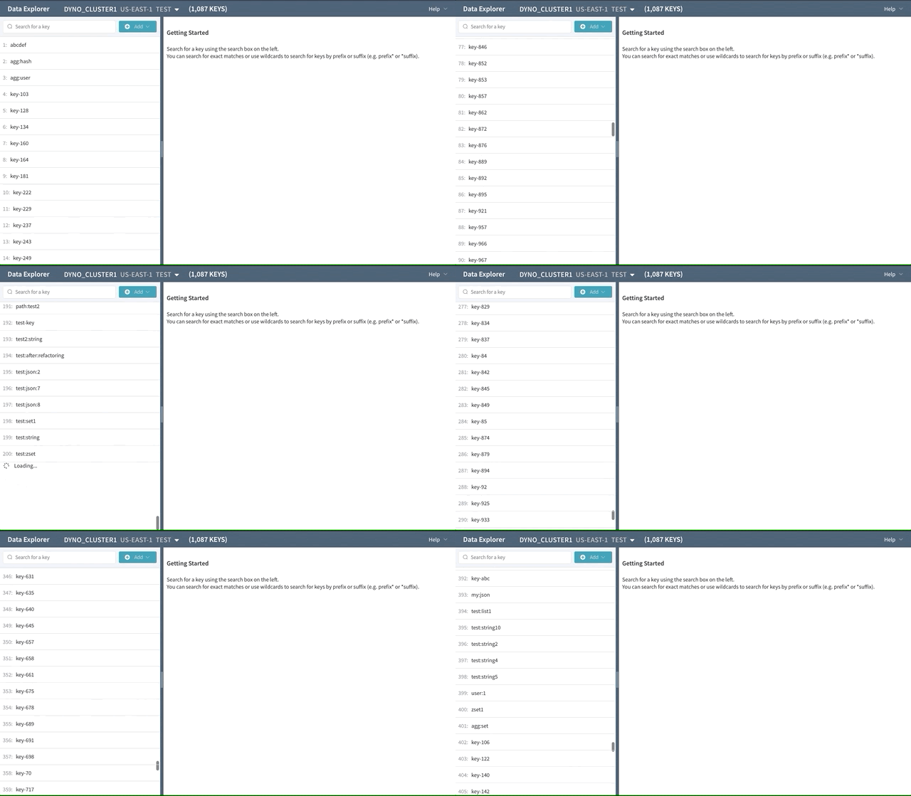
Key Scanning

Since Redis is an in-memory data store, we need to avoid operations that inadvertently load all the keys into memory. We perform SCAN operations across all nodes in the cluster, ensuring we don’t strain the cluster.
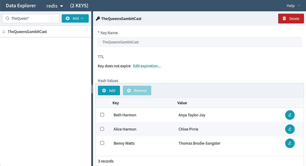
Scanning for keys on a Dynomite cluster

Dynomite Collection Support

In addition to simple String keys, Dynomite supports a rich collection of data types, including Lists, Hashes, and sorted and unsorted Sets. The UI supports creating and manipulating these collection types as well.

Editing a Redis hash value

Supporting OSS

As we were building the Data Explorer, we started getting some strong signals that the ease-of-use and productivity gains that we’d seen internally would benefit folks outside of Netflix as well. We tried to balance codifying some hard-learned best practices that would be generally applicable while maintaining the flexibility to support various OSS environments. To that end, we’ve built several adapter layers into the product where you can provide custom implementations as needed.

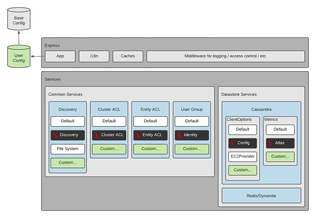
The application was architected to enable OSS by introducing seams where users could provide their implementations for discovery, access control, and data store-specific connection settings. Users can choose one of the built-in service providers or supply a custom provider.

The diagram below shows the server-side architecture. The server is a Node.js Express application written in TypeScript, and the client is a Single Page App written in Vue.js.

Data Explorer architecture and service adapter layers

Demo Environment

Deploying a new tool in any real-world environment is a time commitment. We get it, and to help you with that initial setup, we have included a dockerized demo environment. It can build the app, pull down images for Cassandra and Redis, and run everything in Docker containers so you can dive right in. Note, the demo environment is not intended for production use.

Overridable Configuration

The Data Explorer ships with many default behaviors, but since no two production environments are alike, we provide a mechanism to override the defaults and specify your custom values for various settings. These can range from which port numbers to use to which features should be disabled in a production environment. (For example, the ability to drop a Cassandra table.)

CLI Setup Tool

To further improve the experience of creating your configuration file, we have built a CLI tool that provides a series of prompts for you to follow. The CLI tool is the recommended approach for building your configuration file, and you can re-run the tool at any point to create a new configuration.

The CLI allows you to create a custom configuration

You can also generate multiple configuration files and easily switch between them when working with different environments. We have instructions on GitHub on working with more than one configuration file.

Service Adapters

It’s no secret that Netflix is a big proponent of microservices: we have discovery services for identifying Cassandra and Dynomite clusters in the environment; access-control services that identify who owns a data store and who can access it; and LDAP services to find out information about the logged-in user. There’s a good chance you have similar services in your environment too.

To help enable such environments, we have several pre-canned configurations with overridable values and adapter layers in place.

Discovery

The first example of this adapter layer in action is how the application finds Discovery information — these are the names and IP addresses of the clusters you want to access. The CLI allows you to choose from a few simple options. For instance, if you have a process that can update a JSON file on disk, you can select “file system.” If instead, you have a REST-based microservice that provides this information, then you can choose “custom” and write a few lines of code necessary to fetch it.

Choosing to discover our data store clusters by reading a local file

Metrics

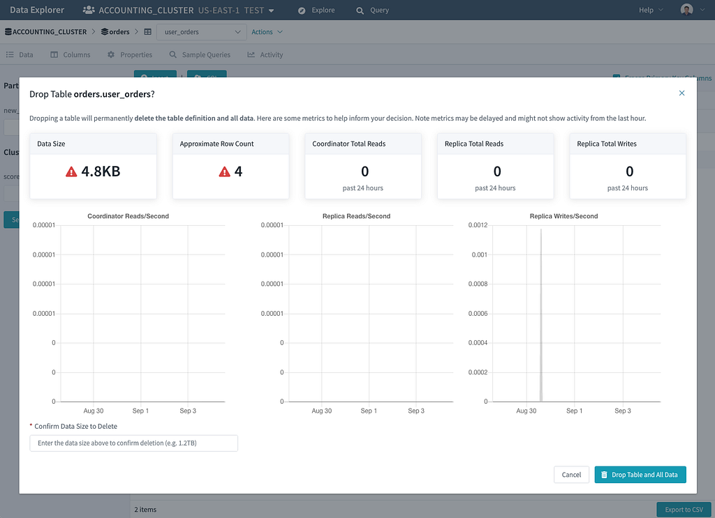
Another example of this service adapter layer is integration with an external metrics service. We progressively enhance the UI by displaying keyspace and table metrics by implementing a metrics service adapter. These metrics provide insight into which tables are being used at a glance and help our customers make an informed decision when dropping a table.

Without metrics support
With optional metrics support

OSS users can enable the optional Metrics support via the CLI. You then just need to write the custom code to fetch the metrics.

CLI enabling customization of advanced features

i18n Support

While internationalization wasn’t an explicit goal, we discovered that providing Netflix-specific messages in some instances yielded additional value to our internal users. Fundamentally, this is similar to how resource bundles handle different locales.

We are making en-NFLX.ts available internally and en-US.ts available externally. Enterprise customers can enhance their user’s experience by creating custom resource bundles (en-ACME.ts) that link to other tools or enhance default messages. Only a small percentage of the UI and server-side exceptions use these message bundles currently — most commonly to augment messages somehow (e.g., provide links to internal slack channels).
Final Thoughts

We invite you to check out the project and let us know how it works for you. By sharing the Netflix Data Explorer with the OSS community, we hope to help you explore your data and inspire some new ideas.


Exploring Data @ Netflix was originally published in Netflix TechBlog on Medium, where people are continuing the conversation by highlighting and responding to this story.