Tag Archives: Asset management

Elasticsearch Indexing Strategy in Asset Management Platform (AMP)

Post Syndicated from Netflix Technology Blog original https://netflixtechblog.com/elasticsearch-indexing-strategy-in-asset-management-platform-amp-99332231e541

By Burak Bacioglu, Meenakshi Jindal

Asset Management at Netflix

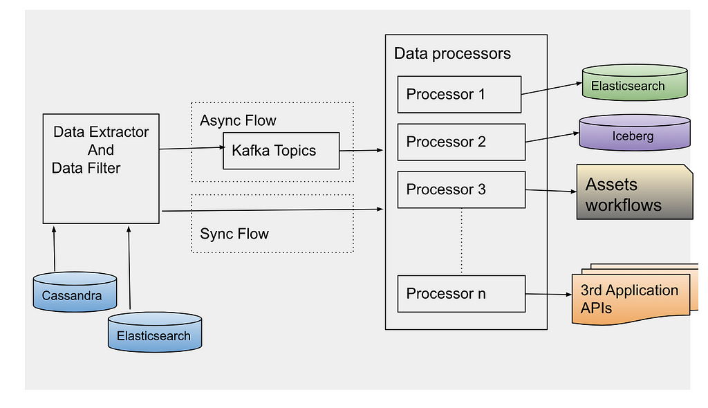
At Netflix, all of our digital media assets (images, videos, text, etc.) are stored in secure storage layers. We built an asset management platform (AMP), codenamed Amsterdam, in order to easily organize and manage the metadata, schema, relations and permissions of these assets. It is also responsible for asset discovery, validation, sharing, and for triggering workflows.

Amsterdam service utilizes various solutions such as Cassandra, Kafka, Zookeeper, EvCache etc. In this blog, we will be focusing on how we utilize Elasticsearch for indexing and search the assets.

Amsterdam is built on top of three storage layers.

The first layer, Cassandra, is the source of truth for us. It consists of close to a hundred tables (column families) , the majority of which are reverse indices to help query the assets in a more optimized way.

The second layer is Elasticsearch, which is used to discover assets based on user queries. This is the layer we’d like to focus on in this blog. And more specifically, how we index and query over 7TB of data in a read-heavy and continuously growing environment and keep our Elasticsearch cluster healthy.

And finally, we have an Apache Iceberg layer which stores assets in a denormalized fashion to help answer heavy queries for analytics use cases.

Elasticsearch Integration

Elasticsearch is one of the best and widely adopted distributed, open source search and analytics engines for all types of data, including textual, numerical, geospatial, structured or unstructured data. It provides simple APIs for creating indices, indexing or searching documents, which makes it easy to integrate. No matter whether you use in-house deployments or hosted solutions, you can quickly stand up an Elasticsearch cluster, and start integrating it from your application using one of the clients provided based on your programming language (Elasticsearch has a rich set of languages it supports; Java, Python, .Net, Ruby, Perl etc.).

One of the first decisions when integrating with Elasticsearch is designing the indices, their settings and mappings. Settings include index specific properties like number of shards, analyzers, etc. Mapping is used to define how documents and their fields are supposed to be stored and indexed. You define the data types for each field, or use dynamic mapping for unknown fields. You can find more information on settings and mappings on Elasticsearch website.

Most applications in content and studio engineering at Netflix deal with assets; such as videos, images, text, etc. These applications are built on a microservices architecture, and the Asset Management Platform provides asset management to those dozens of services for various asset types. Each asset type is defined in a centralized schema registry service responsible for storing asset type taxonomies and relationships. Therefore, it initially seemed natural to create a different index for each asset type. When creating index mappings in Elasticsearch, one has to define the data type for each field. Since different asset types could potentially have fields with the same name but with different data types; having a separate index for each type would prevent such type collisions. Therefore we created around a dozen indices per asset type with fields mapping based on the asset type schema. As we onboarded new applications to our platform, we kept creating new indices for the new asset types. We have a schema management microservice which is used to store the taxonomy of each asset type; and this programmatically created new indices whenever new asset types were created in this service. All the assets of a specific type use the specific index defined for that asset type to create or update the asset document.

Fig 1. Indices based on Asset Types

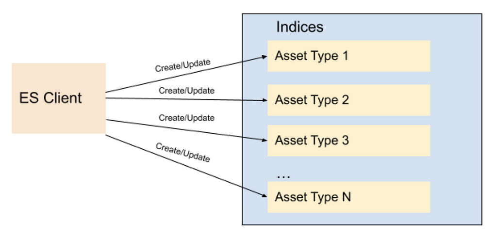
As Netflix is now producing significantly more originals than it used to when we started this project a few years ago, not only did the number of assets grow dramatically but also the number of asset types grew from dozens to several thousands. Hence the number of Elasticsearch indices (per asset type) as well as asset document indexing or searching RPS (requests per second) grew over time. Although this indexing strategy worked smoothly for a while, interesting challenges started coming up and we started to notice performance issues over time. We started to observe CPU spikes, long running queries, instances going yellow/red in status.

Usually the first thing to try is to scale up the Elasticsearch cluster horizontally by increasing the number of nodes or vertically by upgrading instance types. We tried both, and in many cases it helps, but sometimes it is a short term fix and the performance problems come back after a while; and it did for us. You know it is time to dig deeper to understand the root cause of it.

It was time to take a step back and reevaluate our ES data indexing and sharding strategy. Each index was assigned a fixed number of 6 shards and 2 replicas (defined in the template of the index). With the increase in the number of asset types, we ended up having approximately 900 indices (thus 16200 shards). Some of these indices had millions of documents, whereas many of them were very small with only thousands of documents. We found the root cause of the CPU spike was unbalanced shards size. Elasticsearch nodes storing those large shards became hot spots and queries hitting those instances were timing out or very slow due to busy threads.

We changed our indexing strategy and decided to create indices based on time buckets, rather than asset types. What this means is, assets created between t1 and t2 would go to the T1 bucket, assets created between t2 and t3 would go to the T2 bucket, and so on. So instead of persisting assets based on their asset types, we would use their ids (thus its creation time; because the asset id is a time based uuid generated at the asset creation) to determine which time bucket the document should be persisted to. Elasticsearch recommends each shard to be under 65GB (AWS recommends them to be under 50GB), so we could create time based indices where each index holds somewhere between 16–20GB of data, giving some buffer for data growth. Existing assets can be redistributed appropriately to these precreated shards, and new assets would always go to the current index. Once the size of the current index exceeds a certain threshold (16GB), we would create a new index for the next bucket (minute/hour/day) and start indexing assets to the new index created. We created an index template in Elasticsearch so that the new indices always use the same settings and mappings stored in the template.

We chose to index all versions of an asset in the the same bucket – the one that keeps the first version. Therefore, even though new assets can never be persisted to an old index (due to our time based id generation logic, they always go to the latest/current index); existing assets can be updated, causing additional documents for those new asset versions to be created in those older indices. Therefore we chose a lower threshold for the roll over so that older shards would still be well under 50GB even after those updates.

Fig 2. Indices based on Time Buckets

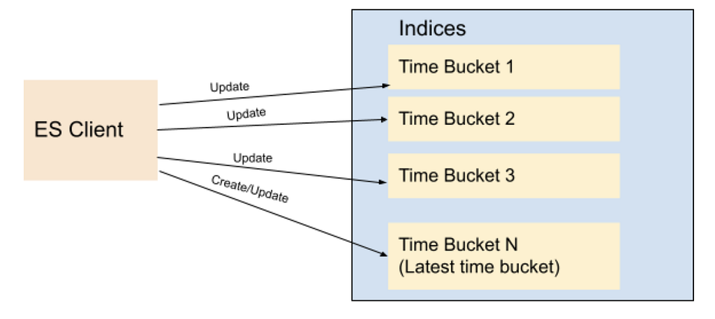
For searching purposes, we have a single read alias that points to all indices created. When performing a query, we always execute it on the alias. This ensures that no matter where documents are, all documents matching the query will be returned. For indexing/updating documents, though, we cannot use an alias, we use the exact index name to perform index operations.

To avoid the ES query for the list of indices for every indexing request, we keep the list of indices in a distributed cache. We refresh this cache whenever a new index is created for the next time bucket, so that new assets will be indexed appropriately. For every asset indexing request, we look at the cache to determine the corresponding time bucket index for the asset. The cache stores all time-based indices in a sorted order (for simplicity we named our indices based on their starting time in the format yyyyMMddHHmmss) so that we can easily determine exactly which index should be used for asset indexing based on the asset creation time. Without using the time bucket strategy, the same asset could have been indexed into multiple indices because Elasticsearch doc id is unique per index and not the cluster. Or we would have to perform two API calls, first to identify the specific index and then to perform the asset update/delete operation on that specific index.

It is still possible to exceed 50GB in those older indices if millions of updates occur within that time bucket index. To address this issue, we added an API that would split an old index into two programmatically. In order to split a given bucket T1 (which stores all assets between t1 and t2) into two, we choose a time t1.5 between t1 and t2, create a new bucket T1_5, and reindex all assets created between t1.5 and t2 from T1 into this new bucket. While the reindexing is happening, queries / reads are still answered by T1, so any new document created (via asset updates) would be dual-written into T1 and T1.5, provided that their timestamp falls between t1.5 and t2. Finally, once the reindexing is complete, we enable reads from T1_5, stop the dual write and delete reindexed documents from T1.

In fact, Elasticsearch provides an index rollover feature to handle the growing indicex problem https://www.elastic.co/guide/en/elasticsearch/reference/6.0/indices-rollover-index.html. With this feature, a new index is created when the current index size hits a threshold, and through a write alias, the index calls will point to the new index created. That means, all future index calls would go to the new index created. However, this would create a problem for our update flow use case, because we would have to query multiple indices to determine which index contains a particular document so that we can update it appropriately. Because the calls to Elasticsearch may not be sequential, meaning, an asset a1 created at T1 can be indexed after another asset a2 created at T2 where T2>T1, the older asset a1 can end up in the newer index while the newer asset a2 is persisted in the old index. In our current implementation, however, by simply looking at the asset id (and asset creation time), we can easily find out which index to go to and it is always deterministic.

One thing to mention is, Elasticsearch has a default limit of 1000 fields per index. If we index all types to a single index, wouldn’t we easily exceed this number? And what about the data type collisions we mentioned above? Having a single index for all data types could potentially cause collisions when two asset types define different data types for the same field. We also changed our mapping strategy to overcome these issues. Instead of creating a separate Elasticsearch field for each metadata field defined in an asset type, we created a single nested type with a mandatory field called `key`, which represents the name of the field on the asset type, and a handful of data-type specific fields, such as: `string_value`, `long_value`, `date_value`, etc. We would populate the corresponding data-type specific field based on the actual data type of the value. Below you can see a part of the index mapping defined in our template, and an example from a document (asset) which has four metadata fields:

Fig 3. Snippet of the index mapping
Fig 4. Snippet of nested metadata field on a stored document

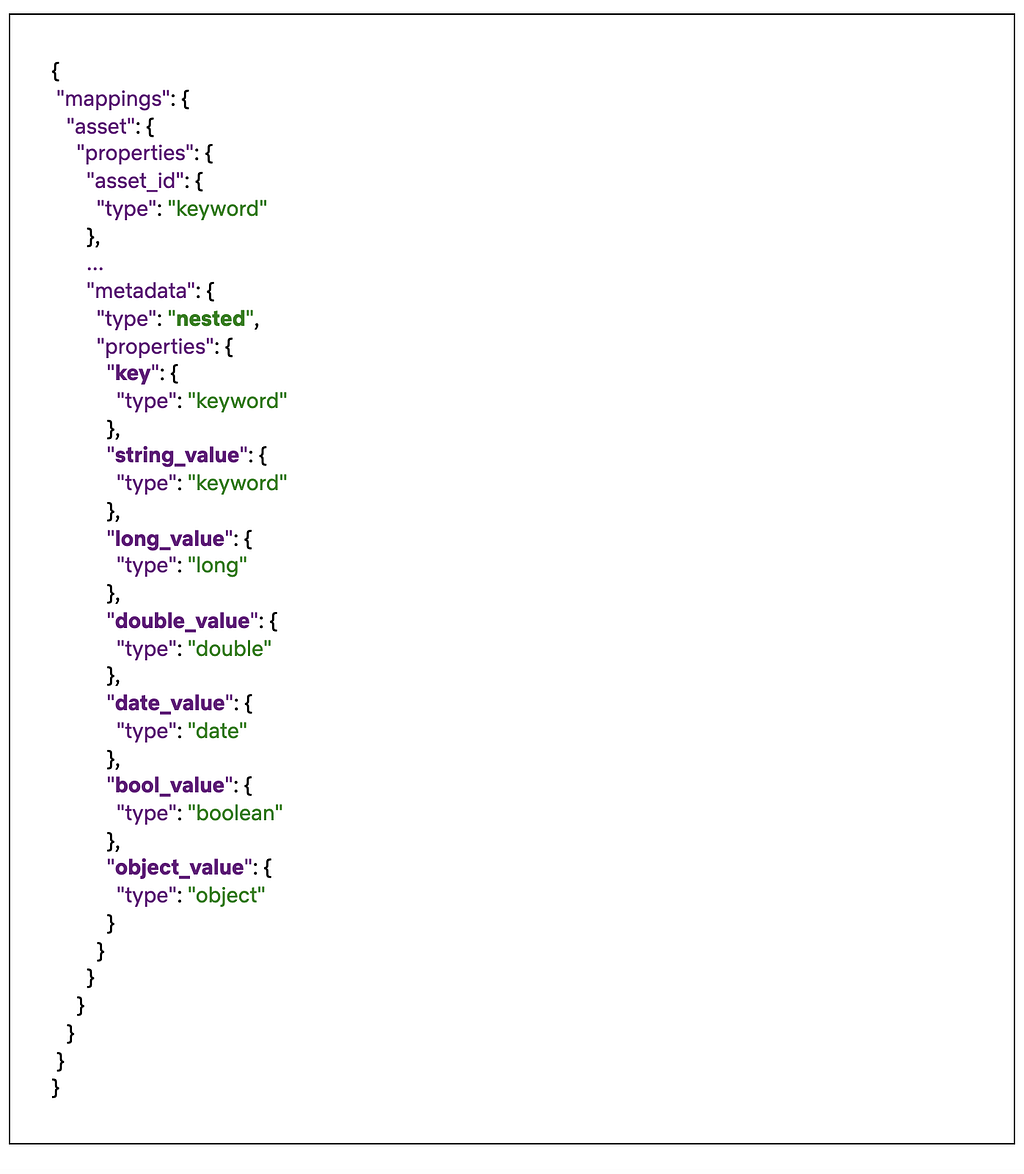
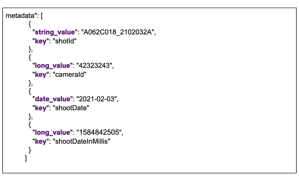
As you see above, all asset properties go under the same nested field `metadata` with a mandatory `key` field, and the corresponding data-type specific field. This ensures that no matter how many asset types or properties are indexed, we would always have a fixed number of fields defined in the mapping. When searching for these fields, instead of querying for a single value (cameraId == 42323243), we perform a nested query where we query for both key and the value (key == cameraId AND long_value == 42323243). For more information on nested queries, please refer to this link.

Fig 5. Search/Indexing RPS

After these changes, the indices we created are now balanced in terms of data size. CPU utilization is down from an average of 70% to 10%. In addition, we are able to reduce the refresh interval time on these indices from our earlier setting 30 seconds to 1 sec in order to support use cases like read after write, which enables users to search and get a document after a second it was created

Fig 6. CPU Spike with Old indexing strategy
Fig 7. CPU Usage with New indexing strategy

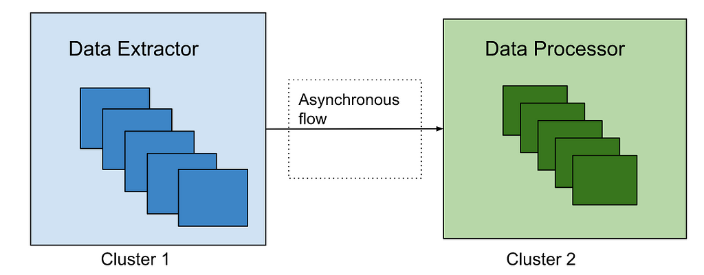
We had to do a one time migration of the existing documents to the new indices. Thankfully we already have a framework in place that can query all assets from Cassandra and index them in Elasticsearch. Since doing full table scans in Cassandra is not generally recommended on large tables (due to potential timeouts), our cassandra schema contains several reverse indices that help us query all data efficiently. We also utilize Kafka to process these assets asynchronously without impacting our real time traffic. This infrastructure is used not only to index assets to Elasticsearch, but also to perform administrative operations on all or some assets, such as bulk updating assets, scanning / fixing problems on them, etc. Since we only focused on Elasticsearch indexing in this blog, we are planning to create another blog to talk about this infrastructure later.


Elasticsearch Indexing Strategy in Asset Management Platform (AMP) was originally published in Netflix TechBlog on Medium, where people are continuing the conversation by highlighting and responding to this story.

Data Reprocessing Pipeline in Asset Management Platform @Netflix

Post Syndicated from Netflix Technology Blog original https://netflixtechblog.com/data-reprocessing-pipeline-in-asset-management-platform-netflix-46fe225c35c9

By Meenakshi Jindal

Overview

At Netflix, we built the asset management platform (AMP) as a centralized service to organize, store and discover the digital media assets created during the movie production. Studio applications use this service to store their media assets, which then goes through an asset cycle of schema validation, versioning, access control, sharing, triggering configured workflows like inspection, proxy generation etc. This platform has evolved from supporting studio applications to data science applications, machine-learning applications to discover the assets metadata, and build various data facts.

During this evolution, quite often we receive requests to update the existing assets metadata or add new metadata for the new features added. This pattern grows over time when we need to access and update the existing assets metadata. Hence we built the data pipeline that can be used to extract the existing assets metadata and process it specifically to each new use case. This framework allowed us to evolve and adapt the application to any unpredictable inevitable changes requested by our platform clients without any downtime. Production assets operations are performed in parallel with older data reprocessing without any service downtime. Some of the common supported data reprocessing use cases are listed below.

Production Use Cases

  • Real-Time APIs (backed by the Cassandra database) for asset metadata access don’t fit analytics use cases by data science or machine learning teams. We build the data pipeline to persist the assets data in the iceberg in parallel with cassandra and elasticsearch DB. But to build the data facts, we need the complete data set in the iceberg and not just the new. Hence the existing assets data was read and copied to the iceberg tables without any production downtime.
  • Asset versioning scheme is evolved to support the major and minor version of assets metadata and relations update. This feature support required a significant update in the data table design (which includes new tables and updating existing table columns). Existing data got updated to be backward compatible without impacting the existing running production traffic.
  • Elasticsearch version upgrade which includes backward incompatible changes, so all the assets data is read from the primary source of truth and reindexed again in the new indices.
  • Data Sharding strategy in elasticsearch is updated to provide low search latency (as described in blog post)
  • Design of new Cassandra reverse indices to support different sets of queries.
  • Automated workflows are configured for media assets (like inspection) and these workflows are required to be triggered for old existing assets too.
  • Assets Schema got evolved that required reindexing all assets data again in ElasticSearch to support search/stats queries on new fields.
  • Bulk deletion of assets related to titles for which license is expired.
  • Updating or Adding metadata to existing assets because of some regressions in client application/within service itself.

Data Reprocessing Pipeline Flow

Figure 1. Data Reprocessing Pipeline Flow

Data Extractor

Cassandra is the primary data store of the asset management service. With SQL datastore, it was easy to access the existing data with pagination regardless of the data size. But there is no such concept of pagination with No-SQL datastores like Cassandra. Some features are provided by Cassandra (with newer versions) to support pagination like pagingstate, COPY, but each one of them has some limitations. To avoid dependency on data store limitations, we designed our data tables such that the data can be read with pagination in a performant way.

Mainly we read the assets data either by asset schema types or time bucket based on asset creation time. Data sharding completely based on the asset type may have created the wide rows considering some types like VIDEO may have many more assets compared to others like TEXT. Hence, we used the asset types and time buckets based on asset creation date for data sharding across the Cassandra nodes. Following is the example of tables primary and clustering keys defined:

Figure 2. Cassandra Table Design

Based on the asset type, first time buckets are fetched which depends on the creation time of assets. Then using the time buckets and asset types, a list of assets ids in those buckets are fetched. Asset Id is defined as a cassandra Timeuuid data type. We use Timeuuids for AssetId because it can be sorted and then used to support pagination. Any sortable Id can be used as the table primary key to support the pagination. Based on the page size e.g. N, first N rows are fetched from the table. Next page is fetched from the table with limit N and asset id < last asset id fetched.

Figure 3. Cassandra Data Fetch Query

Data layers can be designed based on different business specific entities which can be used to read the data by those buckets. But the primary id of the table should be sortable to support the pagination.

Sometimes we have to reprocess a specific set of assets only based on some field in the payload. We can use Cassandra to read assets based on time or an asset type and then further filter from those assets which satisfy the user’s criteria. Instead we use Elasticsearch to search those assets which are more performant.

After reading the asset ids using one of the ways, an event is created per asset id to be processed synchronously or asynchronously based on the use case. For asynchronous processing, events are sent to Apache Kafka topics to be processed.

Data Processor

Data processor is designed to process the data differently based on the use case. Hence, different processors are defined which can be extended based on the evolving requirements. Data can be processed synchronously or asynchronously.

Synchronous Flow: Depending on the event type, the specific processor can be directly invoked on the filtered data. Generally, this flow is used for small datasets.

Asynchronous Flow: Data processor consumes the data events sent by the data extractor. Apache Kafka topic is configured as a message broker. Depending on the use case, we have to control the number of events processed in a time unit e.g. to reindex all the data in elasticsearch because of template change, it is preferred to re-index the data at certain RPS to avoid any impact on the running production workflow. Async processing has the benefit to control the flow of event processing with Kafka consumers count or with controlling thread pool size on each consumer. Event processing can also be stopped at any time by disabling the consumers in case production flow gets any impact with this parallel data processing. For fast processing of the events, we use different settings of Kafka consumer and Java executor thread pool. We poll records in bulk from Kafka topics, and process them asynchronously with multiple threads. Depending on the processor type, events can be processed at high scale with right settings of consumer poll size and thread pool.

Each of these use cases mentioned above looks different, but they all need the same reprocessing flow to extract the old data to be processed. Many applications design data pipelines for the processing of the new data; but setting up such a data processing pipeline for the existing data supports handling the new features by just implementing a new processor. This pipeline can be thoughtfully triggered anytime with the data filters and data processor type (which defines the actual action to be performed).

Error Handling

Errors are part of software development. But with this framework, it has to be designed more carefully as bulk data reprocessing will be done in parallel with the production traffic. We have set up the different clusters of data extractor and processor from the main Production cluster to process the older assets data to avoid any impact of the assets operations live in production. Such clusters may have different configurations of thread pools to read and write data from database, logging levels and connection configuration with external dependencies.

Figure 4: Processing clusters

Data processors are designed to continue processing the events even in case of some errors for eg. There are some unexpected payloads in old data. In case of any error in the processing of an event, Kafka consumers acknowledge that event is processed and send those events to a different queue after some retries. Otherwise Kafka consumers will continue trying to process the same message again and block the processing of other events in the topic. We reprocess data in the dead letter queue after fixing the root cause of the issue. We collect the failure metrics to be checked and fixed later. We have set up the alerts and continuously monitor the production traffic which can be impacted because of the bulk old data reprocessing. In case any impact is noticed, we should be able to slow down or stop the data reprocessing at any time. With different data processor clusters, this can be easily done by reducing the number of instances processing the events or reducing the cluster to 0 instances in case we need a complete halt.

Best Practices

  • Depending on existing data size and use case, processing may impact the production flow. So identify the optimal event processing limits and accordingly configure the consumer threads.
  • If the data processor is calling any external services, check the processing limits of those services because bulk data processing may create unexpected traffic to those services and cause scalability/availability issues.
  • Backend processing may take time from seconds to minutes. Update the Kafka consumer timeout settings accordingly otherwise different consumer may try to process the same event again after processing timeout.
  • Verify the data processor module with a small data set first, before trigger processing of the complete data set.
  • Collect the success and error processing metrics because sometimes old data may have some edge cases not handled correctly in the processors. We are using the Netflix Atlas framework to collect and monitor such metrics.

Acknowledgements

Burak Bacioglu and other members of the Asset Management platform team have contributed in the design and development of this data reprocessing pipeline.


Data Reprocessing Pipeline in Asset Management Platform @Netflix was originally published in Netflix TechBlog on Medium, where people are continuing the conversation by highlighting and responding to this story.

Disaster recovery compliance in the cloud, part 2: A structured approach

Post Syndicated from Dan MacKay original https://aws.amazon.com/blogs/security/disaster-recovery-compliance-in-the-cloud-part-2-a-structured-approach/

Compliance in the cloud is fraught with myths and misconceptions. This is particularly true when it comes to something as broad as disaster recovery (DR) compliance where the requirements are rarely prescriptive and often based on legacy risk-mitigation techniques that don’t account for the exceptional resilience of modern cloud-based architectures. For regulated entities subject to principles-based supervision such as many financial institutions (FIs), the responsibility lies with the FI to determine what’s necessary to adequately recover from a disaster event. Without clear instructions, FIs are susceptible to making incorrect assumptions regarding their compliance requirements for DR.

In Part 1 of this two-part series, I provided some examples of common misconceptions FIs have about compliance requirements for disaster recovery in the cloud. In Part 2, I outline five steps you can take to avoid these misconceptions when architecting DR-compliant workloads for deployment on Amazon Web Services (AWS).

1. Identify workloads planned for deployment

It’s common for FIs to have a portfolio of workloads they are considering deploying to the cloud and often want to know that they can be compliant across the board. But compliance isn’t a one-size-fits-all domain—it’s based on the characteristics of each workload. For example, does the workload contain personally identifiable information (PII)? Will it be used to store, process, or transmit credit card information? Compliance is dependent on the answers to questions such as these and must be assessed on a case-by-case basis. Therefore, the first step in architecting for compliance is to identify the specific workloads you plan to deploy to the cloud. This way, you can assess the requirements of these specific workloads and not be distracted by aspects of compliance that might not be relevant.

2. Define the workload’s resiliency requirements

Resiliency is the ability of a workload to recover from infrastructure or service disruptions. DR is an important part of your resiliency strategy and concerns how your workload responds to a disaster event. DR strategies on AWS range from simple, low cost options such as backup and restore, to more complex options such as multi-site active-active, as shown in Figure 1.
 

For more information, I encourage you to read Seth Eliot’s blog series on DR Architecture on AWS as well as the AWS whitepaper Disaster Recovery of Workloads on AWS: Recovery in the Cloud.

The DR strategy you choose for a particular workload is dependent on your organization’s requirements for avoiding loss of data—known as the recovery point objective (RPO)—and reducing downtime where the workload isn’t available —known as the recovery time objective (RTO). RPO and RTO are key factors for determining the minimum architectural specifications necessary to meet the workload’s resiliency requirements. For example, can the workload’s RPO and RTO be achieved using a multi-AZ architecture in a single AWS Region, or do the resiliency requirements necessitate deploying the workload across multiple AWS Regions? Even if your workload is not subject to explicit compliance requirements for resiliency, understanding these requirements is necessary for assessing other aspects of DR compliance, including data residency and geodiversity.

3. Confirm the workload’s data residency requirements

As I mentioned in Part 1, data residency requirements might restrict which AWS Region or Regions you can deploy your workload to. Therefore, you need to confirm whether the workload is subject to any data residency requirements within applicable laws and regulations, corporate policies, or contractual obligations.

In order to properly assess these requirements, you must review the explicit language of the requirements so as to understand the specific constraints they impose. You should also consult legal, privacy, and compliance subject-matter specialists to help you interpret these requirements based on the characteristics of the workload. For example, do the requirements specifically state that the data cannot leave the country, or can the requirement be met so long as the data can be accessed from that country? Does the requirement restrict you from storing a copy of the data in another country—for example, for backup and recovery purposes? What if the data is encrypted and can only be read using decryption keys kept within the home country? Consulting subject-matter specialists to help interpret these requirements can help you avoid making overly restrictive assumptions and imposing unnecessary constraints on the workload’s architecture.

4. Confirm the workload’s geodiversity requirements

A single Region, multiple-AZ architecture is often sufficient to meet a workload’s resiliency requirements. However, if the workload is subject to geodiversity requirements, the distance between the AZs in an AWS Region might not conform to the minimum distance between individual data centers specified by the requirements. Therefore, it’s critical to confirm whether any geodiversity requirements apply to the workload.

Like data residency, it’s important to assess the explicit language of geodiversity requirements. Are they written down in a regulation or corporate policy, or are they just a recommended practice? Can the requirements be met if the workload is deployed across three or more AZs even if the minimum distance between those AZs is less than the specified minimum distance between the primary and backup data centers? If it’s a corporate policy, does it allow for exceptions if an alternative method provides equal or greater resiliency than asynchronous replication between two geographically distant data centers? Or perhaps the corporate policy is outdated and should be revised to reflect modern risk mitigation techniques. Understanding these parameters can help you avoid unnecessary constraints as you assess architectural options for your workloads.

5. Assess architectural options to meet the workload’s requirements

Now that you understand the workload’s requirements for resiliency, data residency, and geodiversity, you can assess the architectural options that meet these requirements in the cloud.

As per AWS Well-Architected best practices, you should strive for the simplest architecture necessary to meet your requirements. This includes assessing whether the workload can be accommodated within a single AWS Region. If the workload is constrained by explicit geographic diversity requirements or has resiliency requirements that cannot be accommodated by a single AWS Region, then you might need to architect the workload for deployment across multiple AWS Regions. If the workload is also constrained by explicit data residency requirements, then it might not be possible to deploy to multiple AWS Regions. In cases such as these, you can work with our AWS Solution Architects to assess hybrid options that might meet your compliance requirements, such as using AWS Outposts, Amazon Elastic Container Service (Amazon ECS) Anywhere, or Amazon Elastic Kubernetes Service (Amazon EKS) Anywhere. Another option may be to consider a DR solution in which your on-premises infrastructure is used as a backup for a workload running on AWS. In some cases, this might be a long-term solution. In others, it might be an interim solution until certain constraints can be removed—for example, a change to corporate policy or the introduction of additional AWS Regions in a particular country.

Conclusion

Let’s recap by summarizing some guiding principles for architecting compliant DR workloads as outlined in this two-part series:

  • Avoid assumptions; confirm the facts. If it’s not written down, it’s unlikely to be considered a mandatory compliance requirement.
  • Consult the experts. Legal, privacy, and compliance, as well as AWS Solution Architects, AWS security and compliance specialists, and other subject-matter specialists.
  • Avoid generalities; focus on the specifics. There is no one-size-fits-all approach.
  • Strive for simplicity, not zero risk. Don’t use multiple AWS Regions when one will suffice.
  • Don’t get distracted by exceptions. Focus on your current requirements, not workloads you’re not yet prepared to deploy to the cloud.

If you have feedback about this post, submit comments in the Comments section below.

Want more AWS Security how-to content, news, and feature announcements? Follow us on Twitter.

Author

Dan MacKay

Dan is the Financial Services Compliance Specialist for AWS Canada. As a member of the Worldwide Financial Services Security & Compliance team, Dan advises financial services customers on best practices and practical solutions for cloud-related governance, risk, and compliance. He specializes in helping AWS customers navigate financial services and privacy regulations applicable to the use of cloud technology in Canada.

Disaster recovery compliance in the cloud, part 1: Common misconceptions

Post Syndicated from Dan MacKay original https://aws.amazon.com/blogs/security/disaster-recovery-compliance-in-the-cloud-part-1-common-misconceptions/

Compliance in the cloud can seem challenging, especially for organizations in heavily regulated sectors such as financial services. Regulated financial institutions (FIs) must comply with laws and regulations (often in multiple jurisdictions), global security standards, their own corporate policies, and even contractual obligations with their customers and counterparties. These various compliance requirements may impose constraints on how their workloads can be architected for the cloud, and may require interpretation on what FIs must do in order to be compliant. It’s common for FIs to make assumptions regarding their compliance requirements, which can result in unnecessary costs and increased complexity, and might not align with their strategic objectives. A modern, rationalized approach to compliance can help FIs avoid imposing unnecessary constraints while meeting their mandatory requirements.

In my role as an Amazon Web Services (AWS) Compliance Specialist, I work with our financial services customers to identify, assess, and determine solutions to address their compliance requirements as they move to the cloud. One of the most common challenges customers ask me about is how to comply with disaster recovery (DR) requirements for workloads they plan to run in the cloud. In this blog post, I share some of the typical misconceptions FIs have about DR compliance in the cloud. In Part 2, I outline a structured approach to designing compliant architectures for your DR workloads. As my primary market is Canada, the examples in this blog post largely pertain to FIs operating in Canada, but the principles and best practices are relevant to regulated organizations in any country.

“Why isn’t there a checklist for compliance in the cloud?”

Compliance requirements are sometimes prescriptive: “if X, then you must do Y.” When requirements are prescriptive, it’s usually clear what you must do in order to be compliant. For example, the Payment Card Industry Data Security Standard (PCI DSS) requirement 8.2.4 obliges companies that process, store, or transmit credit card information to “change user passwords/passphrases at least once every 90 days.” But in the financial services sector, compliance requirements for managing operational risks can be subjective. When regulators take what is known as a principles-based approach to setting regulatory expectations, each FI is required to assess their specific risks and determine the mitigating controls necessary to conform with the organization’s tolerance for operational risk. Because the rules aren’t prescriptive, there is no “checklist for achieving compliance.” Instead, principles-based requirements are guidelines that FIs are expected to consider as they design and implement technology solutions. They are, by definition, subject to interpretation and can be prone to myths and misconceptions among FIs and their service providers. To illustrate this, let’s look at two aspects of DR that are frequently misunderstood within the Canadian financial services industry: data residency and geodiversity.

“My data has to stay in country X”

Data residency or data localization is a requirement for specific data-sets processed and stored in an IT system to remain within a specific jurisdiction (for example, a country). As discussed in our Policy Perspectives whitepaper, contrary to historical perspectives, data residency doesn’t provide better security. Most cyber-attacks are perpetrated remotely and attackers aren’t deterred by the physical location of their victims. In fact, data residency can run counter to an organization’s objectives for security and resilience. For example, data residency requirements can limit the options our customers have when choosing the AWS Region or Regions in which to run their production workloads. This is especially challenging for customers who want to use multiple Regions for backup and recovery purposes.

It’s common for FIs operating in Canada to assume that they’re required to keep their data—particularly customer data—in Canada. In reality, there’s very little from a statutory perspective that imposes such a constraint. None of the private sector privacy laws include data residency requirements, nor do any of the financial services regulatory guidelines. There are some place of records requirements in Canadian federal financial services legislation such as The Bank Act and The Insurance Companies Act, but these are relatively narrow in scope and apply primarily to corporate records. For most Canadian FIs, their requirements are more often a result of their own corporate policies or contractual obligations, not externally imposed by public policies or regulations.

“My data centers have to be X kilometers apart”

Geodiversity—short for geographic diversity—is the concept of maintaining a minimum distance between primary and backup data processing sites. Geodiversity is based on the principle that requiring a certain distance between data centers mitigates the risk of location-based disruptions such as natural disasters. The principle is still relevant in a cloud computing context, but is not the only consideration when it comes to planning for DR. The cloud allows FIs to define operational resilience requirements instead of limiting themselves to antiquated business continuity planning and DR concepts like physical data center implementation requirements. Legacy disaster recovery solutions and architectures, and lifting and shifting such DR strategies into the cloud, can diminish the potential benefits of using the cloud to improve operational resilience. Modernizing your information technology also means modernizing your organization’s approach to DR.

In the cloud, vast physical distance separation is an anti-pattern—it’s an arbitrary metric that does little to help organizations achieve availability and recovery objectives. At AWS, we design our global infrastructure so that there’s a meaningful distance between the Availability Zones (AZs) within an AWS Region to support high availability, but close enough to facilitate synchronous replication across those AZs (an AZ being a cluster of data centers). Figure 1 shows the relationship between Regions, AZs, and data centers.
 

Synchronous replication across multiple AZs enables you to minimize data loss (defined as the recovery point objective or RPO) and reduce the amount of time that workloads are unavailable (defined as the recovery time objective or RTO). However, the low latency required for synchronous replication becomes less achievable as the distance between data centers increases. Therefore, a geodiversity requirement that mandates a minimum distance between data centers that’s too far for synchronous replication might prohibit you from taking advantage of AWS’s multiple-AZ architecture. A multiple-AZ architecture can achieve RTOs and RPOs that aren’t possible with a simple geodiversity mitigation strategy. For more information, refer to the AWS whitepaper Disaster Recovery of Workloads on AWS: Recovery in the Cloud.

Again, it’s a common perception among Canadian FIs that the disaster recovery architecture for their production workloads must comply with specific geodiversity requirements. However, there are no statutory requirements applicable to FIs operating in Canada that mandate a minimum distance between data centers. Some FIs might have corporate policies or contractual obligations that impose geodiversity requirements, but for most FIs I’ve worked with, geodiversity is usually a recommended practice rather than a formal policy. Informal corporate guidelines can have some value, but they aren’t absolute rules and shouldn’t be treated the same as mandatory compliance requirements. Otherwise, you might be unintentionally restricting yourself from taking advantage of more effective risk management techniques.

“But if it is a compliance requirement, doesn’t that mean I have no choice?”

Both of the previous examples illustrate the importance of not only confirming your compliance requirements, but also recognizing the source of those requirements. It might be infeasible to obtain an exception to an externally-imposed obligation such as a regulatory requirement, but exceptions or even revisions to corporate policies aren’t out of the question if you can demonstrate that modern approaches provide equal or greater protection against a particular risk—for example, the high availability and rapid recoverability supported by a multiple-AZ architecture. Consider whether your compliance requirements provide for some level of flexibility in their application.

Also, because many of these requirements are principles-based, they might be subject to interpretation. You have to consider the specific language of the requirement in the context of the workload. For example, a data residency requirement might not explicitly prohibit you from storing a copy of the content in another country for backup and recovery purposes. For this reason, I recommend that you consult applicable specialists from your legal, privacy, and compliance teams to aid in the interpretation of compliance requirements. Once you understand the legal boundaries of your compliance requirements, AWS Solutions Architects and other financial services industry specialists such as myself can help you assess viable options to meet your needs.

Conclusion

In this first part of a two-part series, I provided some examples of common misconceptions FIs have about compliance requirements for disaster recovery in the cloud. The key is to avoid making assumptions that might impose greater constraints on your architecture than are necessary. In Part 2, I show you a structured approach for architecting compliant DR workloads that can help you to avoid these preventable missteps.

If you have feedback about this post, submit comments in the Comments section below.

Want more AWS Security how-to content, news, and feature announcements? Follow us on Twitter.

Author

Dan MacKay

Dan is the Financial Services Compliance Specialist for AWS Canada. As a member of the Worldwide Financial Services Security & Compliance team, Dan advises financial services customers on best practices and practical solutions for cloud-related governance, risk, and compliance. He specializes in helping AWS customers navigate financial services and privacy regulations applicable to the use of cloud technology in Canada.