Post Syndicated from Grab Tech original https://engineering.grab.com/hubble-data-discovery
Imagine a world where finding the right data is like searching for a needle in a haystack. In today’s data-driven landscape, companies are drowning in a sea of information, struggling to navigate through countless datasets to uncover valuable insights. At Grab, we faced a similar challenge. With over 200,000 tables in our data lake, along with numerous Kafka streams, production databases, and ML features, locating the most suitable dataset for our Grabber’s use cases promptly has historically been a significant hurdle.
Problem Space
Our internal data discovery tool, Hubble, built on top of the popular open-source platform Datahub, was primarily used as a reference tool. While it excelled at providing metadata for known datasets, it struggled with true data discovery due to its reliance on Elasticsearch, which performs well for keyword searches but cannot accept and use user-provided context (i.e., it can’t perform semantic search, at least in its vanilla form). The Elasticsearch parameters provided by Datahub out of the box also had limitations: our monthly average click-through rate was only 82%, meaning that in 18% of sessions, users abandoned their searches without clicking on any dataset. This suggested that the search results were not meeting their needs.
Another indispensable requirement for efficient data discovery that was missing at Grab was documentation. Documentation coverage for our data lake tables was low, with only 20% of the most frequently queried tables (colloquially referred to as P80 tables) having existing documentation. This made it difficult for users to understand the purpose and contents of different tables, even when browsing through them on the Hubble UI.
Consequently, data consumers heavily relied on tribal knowledge, often turning to their colleagues via Slack to find the datasets they needed. A survey conducted last year revealed that 51% of data consumers at Grab took multiple days to find the dataset they required, highlighting the inefficiencies in our data discovery process.
To address these challenges and align with Grab’s ongoing journey towards a data mesh architecture, the Hubble team recognised the importance of improving data discovery. We embarked on a journey to revolutionise the way our employees find and access the data they need, leveraging the power of AI and Large Language Models (LLMs).
Vision
Given the historical context, our vision was clear: to remove humans in the data discovery loop by automating the entire process using LLM-powered products. We aimed to reduce the time taken for data discovery from multiple days to mere seconds, eliminating the need for anyone to ask their colleagues data discovery questions ever again.

Goals
To achieve our vision, we set the following goals for ourselves for the first half of 2024:
- Build HubbleIQ: An LLM-based chatbot that could serve as the equivalent of a Lead Data Analyst for data discovery. Just as a lead is an expert in their domain and can guide data consumers to the right dataset, we wanted HubbleIQ to do the same across all domains at Grab. We also wanted HubbleIQ to be accessible where data consumers hang out the most: Slack.
- Improve documentation coverage: A new Lead Analyst joining the team would require extensive documentation coverage of very high quality. Without this, they wouldn’t know what data exists and where. Thus, it was important for us to improve documentation coverage.
- Enhance Elasticsearch: We aimed to tune our Elasticsearch implementation to better meet the requirements of Grab’s data consumers.
A Systematic Path to Success
Step 1: Enhance Elasticsearch
Through clickstream analysis and user interviews, the Hubble team identified four categories of data search queries that were seen either on the Hubble UI or in Slack channels:
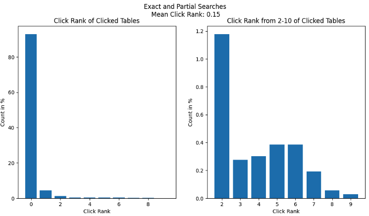
- Exact search: Queries belonging to this category were a substring of an existing dataset’s name at Grab, with the query length being at least 40% of the dataset’s name.
- Partial search: The Levenshtein distance between a query in this category and any existing dataset’s name was greater than 80. This category usually comprised queries that closely resembled an existing dataset name but likely contained spelling mistakes or were shorter than the actual name.
Exact and partial searches accounted for 75% of searches on Hubble (and were non-existent on Slack: as a human, receiving a message that just had the name of a dataset would feel rather odd). Given the effectiveness of vanilla Elasticsearch for these categories, the click rank was close to 0.
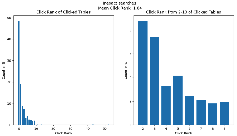
- Inexact search: This category comprised queries that were usually colloquial keywords or phrases that may be semantically related to a given table, column, or piece of documentation (e.g., “city” or “taxi type”). Inexact searches accounted for the remaining 25% of searches on Hubble. Vanilla Elasticsearch did not perform well in this category since it relied on pure keyword matching and did not consider any additional context.
- Semantic search: These were free text queries with abundant contextual information supplied by the user. Hubble did not see any such queries as users rightly expected that Hubble would not be able to fulfil their search needs. Instead, these queries were sent by data consumers to data producers via Slack. Such queries were numerous, but usually resulted in data hunting journeys that spanned multiple days – the root of frustration amongst data consumers.
The first two search types can be seen as “reference” queries, where the data consumer already knows what they are looking for. Inexact and contextual searches are considered “discovery” queries. The Hubble team noticed drop-offs in inexact searches because users learned that Hubble could not fulfil their discovery needs, forcing them to search for alternatives.
Through user interviews, the team discovered how Elasticsearch should be tuned to better fit the Grab context. They implemented the following optimisations:
- Tagging and boosting P80 tables
- Boosting the most relevant schemas
- Hiding irrelevant datasets like PowerBI dataset tables
- Deboosting deprecated tables
- Improving the search UI by simplifying and reducing clutter
- Adding relevant tags
- Boosting certified tables
As a result of these enhancements, the click-through rate rose steadily over the course of the half to 94%, a 12 percentage point increase.
While this helped us make significant improvements to the first three search categories, we knew we had to build HubbleIQ to truly automate the last category – semantic search.
Step 2: Build a Context Store for HubbleIQ
To support HubbleIQ, we built a documentation generation engine that used GPT-4 to generate documentation based on table schemas and sample data. We refined the prompt through multiple iterations of feedback from data producers.
We added a “generate” button on the Hubble UI, allowing data producers to easily generate documentation for their tables. This feature also supported the ongoing Grab-wide initiative to certify tables.
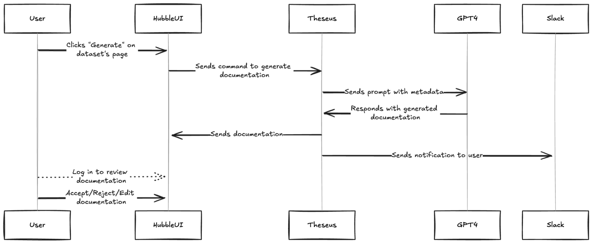
In conjunction, we took the initiative to pre-populate docs for the most critical tables, while notifying data producers to review the generated documentation. Such docs were visible to data consumers with an “AI-generated” tag as a precaution. When data producers accepted or edited the documentation, the tag was removed.
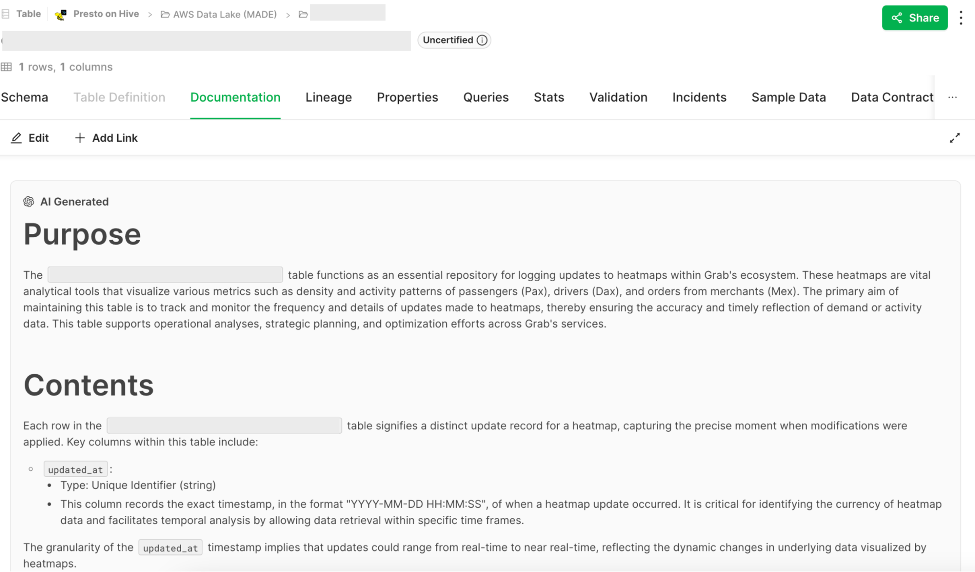
As a result, documentation coverage for P80 tables increased by 70 percentage points to ~90%. User feedback showed that ~95% of users found the generated docs useful.
Step 3: Build and Launch HubbleIQ
With high documentation coverage in place, we were ready to harness the power of LLMs for data discovery. To speed up go-to-market, we decided to leverage Glean, an enterprise search tool used by Grab.
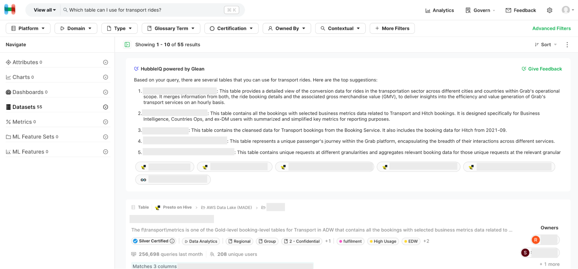
First, we integrated Hubble with Glean, making all data lake tables with documentation available on the Glean platform. Next, we used Glean Apps to create the HubbleIQ bot, which was essentially an LLM with a custom system prompt that could access all Hubble datasets that were catalogued on Glean. Finally, we integrated this bot into Hubble search, such that for any search that is likely to be a semantic search, HubbleIQ results are shown on top, followed by regular search results.
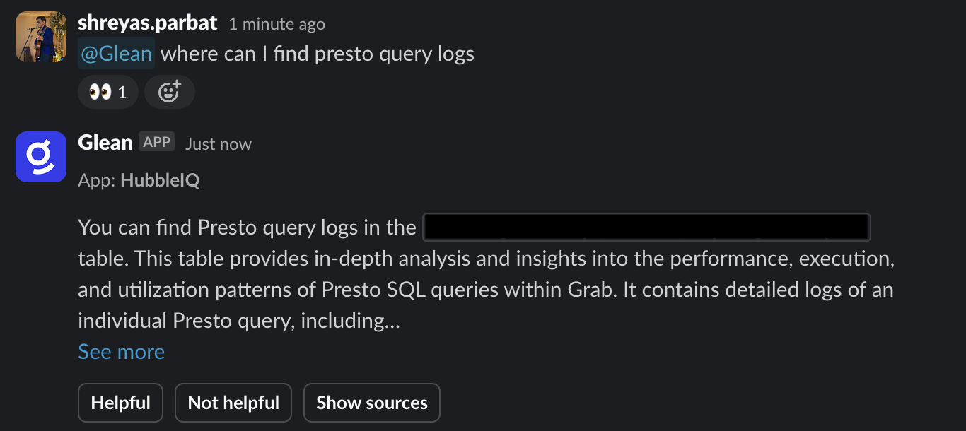
Recently, we integrated HubbleIQ with Slack, allowing data consumers to discover datasets without breaking their flow. Currently, we are working with analytics teams to add the bot to their “ask” channels (where data consumers come to ask contextual search queries for their domains). After integration, HubbleIQ will act as the first line of defence for answering questions in these channels, reducing the need for human intervention.
The impact of these improvements was significant. A follow-up survey revealed that 73% of respondents found it easy to discover datasets, marking a substantial 17 percentage point increase from the previous survey. Moreover, Hubble reached an all-time high in monthly active users, demonstrating the effectiveness of the enhancements made to the platform.
Next Steps
We’ve made significant progress towards our vision, but there’s still work to be done. Looking ahead, we have several exciting initiatives planned to further enhance data discovery at Grab.
On the documentation generation front, we aim to enrich the generator with more context, enabling it to produce even more accurate and relevant documentation. We also plan to streamline the process by allowing analysts to auto-update data docs based on Slack threads directly from Slack. To ensure the highest quality of documentation, we will develop an evaluator model that leverages LLMs to assess the quality of both human and AI-written docs. Additionally, we will implement Reflexion, an agentic workflow that utilises the outputs from the doc evaluator to iteratively regenerate docs until a quality benchmark is met or a maximum try-limit is reached.
As for HubbleIQ, our focus will be on continuous improvement. We’ve already added support for metric datasets and are actively working on incorporating other types of datasets as well. To provide a more seamless user experience, we will enable users to ask follow-up questions to HubbleIQ directly on the HubbleUI, with the system intelligently pulling additional metadata when a user mentions a specific dataset.
Conclusion
By harnessing the power of AI and LLMs, the Hubble team has made significant strides in improving documentation coverage, enhancing search capabilities, and drastically reducing the time taken for data discovery. While our efforts so far have been successful, there are still steps to be taken before we fully achieve our vision of completely replacing the reliance on data producers for data discovery. Nonetheless, with our upcoming initiatives and the groundwork we have laid, we are confident that we will continue to make substantial progress in the right direction over the next few production cycles.
As we forge ahead, we remain dedicated to refining and expanding our AI-powered data discovery tools, ensuring that Grabbers have every dataset they need to drive Grab’s success at their fingertips. The future of data discovery at Grab is brimming with possibilities, and the Hubble team is thrilled to be at the forefront of this exciting journey.
To our readers, we hope that our journey has inspired you to explore how you can leverage the power of AI to transform data discovery within your own organisations. The challenges you face may be unique, but the principles and strategies we have shared can serve as a foundation for your own data discovery revolution. By embracing innovation, focusing on user needs, and harnessing the potential of cutting-edge technologies, you too can unlock the full potential of your data and propel your organisation to new heights. The future of data-driven innovation is here, and we invite you to join us on this exhilarating journey.
Join us
Grab is the leading superapp platform in Southeast Asia, providing everyday services that matter to consumers. More than just a ride-hailing and food delivery app, Grab offers a wide range of on-demand services in the region, including mobility, food, package and grocery delivery services, mobile payments, and financial services across 700 cities in eight countries.
Powered by technology and driven by heart, our mission is to drive Southeast Asia forward by creating economic empowerment for everyone. If this mission speaks to you, join our team today!