Post Syndicated from Grab Tech original https://engineering.grab.com/evalutate-performance-remove-redis-from-scylla-service
Introduction
At Grab, we operate a set of services that manage and provide counts of various items. While this may seem straightforward, the scale at which this feature operates—benefiting millions of Grab users daily—introduces complexity. This feature is divided into three microservices: one for “writing” counts, another for handling “read” requests, and a third serving as the backend for a portal used by data scientists and analysts to configure these counters.
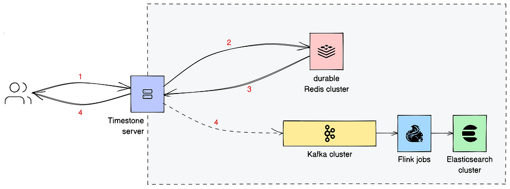
This article focuses on the service responsible for handling “read” requests. This service is backed by Scylla storage and a Redis cache. It also connects to a MySQL RDS to retrieve “counter configurations” that are necessary for processing incoming requests. Written in Rust, the service serves tens of thousands of queries per second (QPS) during peak times, with each request typically being a “batch request” requiring multiple lookups (~10) on Scylla.
Recently, the service has encountered performance challenges, causing periodic spikes in Scylla QPS. These spikes occur throughout the day but are particularly evident during peak hours. To understand this better, we’ll first walk you through how this service operates, particularly how it serves incoming requests. We will then explain our proposed solution and the outcomes of our experiment.
Anatomy of a request
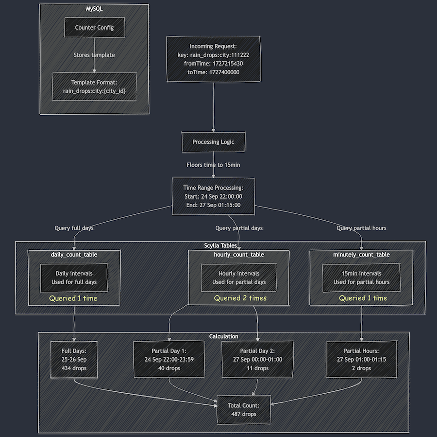
Each counter configuration stored in MySQL has a template that dictates the format of incoming queries. For example, this sample counter configuration is used to count the raindrops for a specific city:
{
    "id": 34,
    "name": "count_rain_drops",
    "template": "rain_drops:city:{city_id}"
    ....
    ....
}
An incoming request using this counter might look like this:
{
    "key": "rain_drops:city:111222",
    "fromTime": 1727215430, // 24 September 2024 22:03:50
    "toTime": 1727400000, // 27 September 2024 01:20:00
}
This request seeks the number of raindrops in our imaginary city with city ID: 111222, between 1727215430 (24 September 2024 22:03:50) and 1727400000 (27 September 2024 01:20:00).
Another service keeps track of raindrops by city and writes the minutely (truncated at 15 minutes), hourly, and daily counts to three different Scylla tables:
- minutely_count_table
- hourly_count_table
- daily_count_table
The service processing the request rounds down the time to the nearest 15 minutes. As a result, the request is processed with the following time range:
- Start time: 24 September 2024 22:00:00
- End time: 27 September 2024 01:15:00
Let’s assume we have the following data in these three tables for “rain_drops:city:111222”. The datapoints used in the above example request are highlighted in bold.
minutely_count_table:
| key | minutely_timestamp | count |
|---|---|---|
| rain_drops:city:111222 | 2024-09-24T22:00:00Z | 3 |
| rain_drops:city:111222 | 2024-09-24T22:15:00Z | 2 |
| rain_drops:city:111222 | 2024-09-24T22:30:00Z | 4 |
| rain_drops:city:111222 | 2024-09-24T22:45:00Z | 1 |
| … | … | … |
| rain_drops:city:111222 | 2024-09-27T01:00:00Z | 2 |
| rain_drops:city:111222 | 2024-09-27T01:15:00Z | 3 |
hourly_count_table:
| key | hourly_timestamp | count |
|---|---|---|
| rain_drops:city:111222 | 2024-09-24T22:00:00Z | 18 |
| rain_drops:city:111222 | 2024-09-24T23:00:00Z | 22 |
| rain_drops:city:111222 | 2024-09-25T00:00:00Z | 15 |
| … | … | … |
| rain_drops:city:111222 | 2024-09-27T00:00:00Z | 11 |
| rain_drops:city:111222 | 2024-09-27T01:00:00Z | 9 |
daily_count_table:
| key | daily_timestamp | count |
|---|---|---|
| rain_drops:city:111222 | 2024-09-24T00:00:00Z | 214 |
| rain_drops:city:111222 | 2024-09-25T00:00:00Z | 189 |
| rain_drops:city:111222 | 2024-09-26T00:00:00Z | 245 |
| rain_drops:city:111222 | 2024-09-27T00:00:00Z | 78 |
Now, let’s see how the service calculates the total count for the incoming request with “rain_drops:city:111222” based on the provided data:
Time range:
- From: 24 September 2024 22:03:50
- To: 27 September 2024 01:20:00
For the full days within the range, specifically 25th and 26th September, we can use data from the daily_count_table. However, for the start (24th September) and end (27th September) date of the range, we cannot use data from the daily_count_table as the range only includes portions of these dates. Instead, we will use a combination of data from the hourly_count_table and minutely_count_table to accurately capture the counts for these days.
-
Query the daily_count_table:
Sum (full day: 25 and 26th Sep): 189 + 245 = 434
- Query the hourly_count_table:
-
For 24th September (from 22:00:00 to 23:59:59):
Hourly count: 18 + 22 = 40
-
For 27th September (from 00:00:00 to 01:00:00):
Hourly count: 11
-
-
Query the minutely_count_table:
For 27th September (from 01:00:00 to 01:15:00):
Minutely count: 2
-
Total count:
Total = Daily count (25th and 26th) + Hourly count (24th) + Hourly count (27th) + Minutely count (27th)
= 434 + 40 + 11 + 2
= 487

As shown in the calculation, when the service receives the request, it comes up with the total count of raindrops by querying three Scylla tables and summing them up using some specific rules within the service itself.
Querying the cache
In the previous section, we explained how Scylla handles a query. If we cached the response for the same request earlier, retrieval from the cache follows a simpler logic. For instance, for the example request, the total count is stored using the floored start and end times (rounded to the nearest 15-minute window within an hour), which was used for the Scylla query instead of the original time in the request. The cache key-value pair would look like this:
- key: id:34:rain_drops:city:111222:1727215200:1727399700
- value: 487
Timestamps 1727215200 and 1727399700 represent the adjusted start and end times of 24 September 2024 22:00:00 and 27 September 2024 01:15:00, respectively. It has a Time-To-Live (TTL) of 5 minutes. During this TTL window, any request for the key “rain_drops:city:111222” having the same start and end times (after rounding to the nearest 15 minutes) will be read from the cache instead of querying Scylla.
For example, for the following three start times, although they are different, after flooring the request to the nearest 15 minutes, the start time becomes 24 September 2024 22:00:00 for all of them, which is the same start time as the one in the cache.
- 24 September 2024 22:01:00
- 24 September 2024 22:02:00
- 24 September 2024 22:06:00
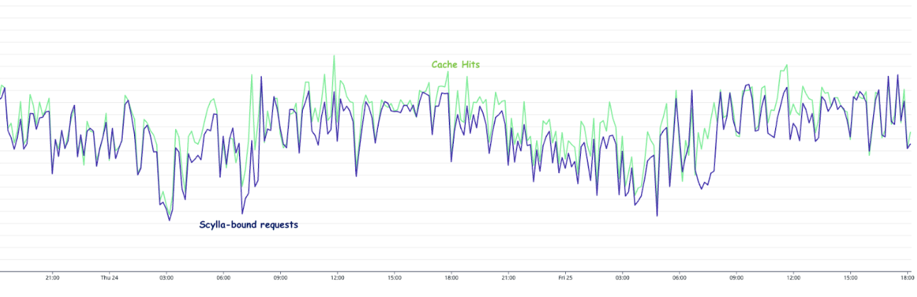
In day-to-day operations, this caching setup allows roughly half of our total production requests to be served by the Redis cache.

Problem statement
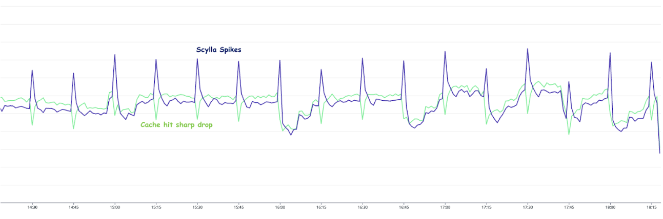
The setup consisting of Scylla and Redis cache works well. Particularly because Scylla-bound queries need to look up 1-3 tables (minutely, hourly, daily, depending on the time range) and perform the summation as explained earlier, whereas a single cache lookup gets the final value for the same query. However, as our cache key pattern follows the 15-minute truncation strategy, along with a 5-minute cache TTL, it leads to an interesting phenomenon – our cache hits plummet and Scylla QPS spikes at the end of every 15 minutes.

This occurs primarily due to the fact that almost all requests to our service are for recent data. Due to this, at the end of every 15-minute block within an hour (i.e., 00, 15, 30, 45), most of the requests require creating new cache keys for the latest 15-minute block. At this point in time, there may be many unexpired (i.e., have not reached 5 min TTL) cache keys from the previous 15-minutes block, but they become less relevant as most requests are asking for recent data.
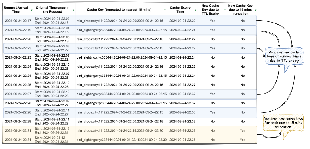
The table in Figure 4 shows example data for configurations “rain_drops:city:111222” and “bird_sighting:city:333444”. For these two configurations, new cache keys are created due to TTL expiry at random times. However, at the end of the 15-minute block, which, in this case is at the end of 22:00-22:15 block, both configurations need new cache keys for the new 15-minute time block that has just started (i.e., start of 22:15-22:30), even though some of their cache keys from the previous 15-minute block are still valid. This requirement of creating new cache keys for most of the requests at the end of a 15-minute block causes spikes in Scylla QPS and a sharp decline in cache hits.
One question that arises is – “Why don’t we see a spike every 5 minutes for cache key TTL expiry?” This is because, within the 15 minutes block, new cache keys are continuously created when a key reaches TTL and a new request for that is received. Since this happens all the time as shown in Figure 4, we do not see a sharp spike. In other words, although Scylla does receive more queries due to cache TTL expiry, it does not lead to a spike in Scylla queries or a sharp drop in cache hits. This is because the cache keys are always being created and invalidated due to TTL expiry instead of following a fixed 5-minute block similar to the 15-minute block we use for our truncation strategy.

These Scylla QPS spikes at the end of every 15-minute block lead to a highly imbalanced Scylla QPS. This often causes high latency in our service during the 15-minute blocks that fall within the peak traffic hours. This further causes more requests to time out, eventually increasing the number of failed requests.
Proposed solution
We propose mitigating this issue by completely removing the Redis-backed caching mechanism from the service. Our observations indicate that the Scylla spikes at the end of 15-minute blocks occur due to cache hit misses. Therefore, removing the caching should eliminate the spikes and provide for a more balanced load.
We acknowledge that this may seem counterintuitive from an overall performance standpoint as removing caching means all queries will be Scylla-bound, potentially impacting the overall performance since caching usually speeds up processes. In addition, caching also comes with an advantage where for cache hits, the service does not need to do the summation on Scylla results from minutely, hourly, and the daily table. Despite these shortcomings, we hypothesise that removing caching should not have an adverse impact on the overall performance. This is based on the fact the Scylla has its own sophisticated caching mechanism. However, our existing setup uses Redis for caching, underutilising Scylla’s cache as the most subsequent queries hit the Redis cache instead.
In summary, we propose eliminating the Redis caching component from our current architecture. This change is expected to resolve the Scylla query spikes observed at the end of every 15-minute block. By relying on Scylla’s native caching mechanism, we anticipate maintaining the service’s overall performance more effectively. The removal of Redis is counterbalanced by the optimised utilisation of Scylla’s built-in caching capabilities.
Experiment
Procedure
The experiment was done on an important live service serving thousands of QPS. To avoid disruptions, we followed a gradual approach. We first turned off caching for a few configurations. If there were no adverse impacts observed, we incrementally disabled cache for more configurations. We controlled the rollout increment by using a mathematical operator on the configuration IDs. This approach is simple and allows us to deterministically disable the cache for specific configurations across all requests, as opposed to using a percentage rollout which randomly disables the cache for different configurations across different requests. This is also due to the fact that the number of configurations is relatively steady and small (less than a thousand). Since these configurations are already fully cached in the service memory from RDS, there will be no performance impact of having a condition that operates on these configurations.
To make sense of the graphs and metrics reported in this section, it is important to understand the traffic pattern of this service. The service usually sees two peaks every day: noon and another around 6-7 PM. On a weekly basis, we usually see the highest traffic on Friday, with the busiest period being from 6-8 PM.
In addition, the timeline of when and how we made various changes to our setup is important to accurately interpret our results.
Experiment timeline: Nov 5 – Nov 13, 2024:
-
Redis cache disabled for ~5% of the counter configurations – Nov 5, 2024, 10.26 AM (Canary started: 10.00 AM)
-
Redis cache disabled for ~25% of the counter configurations – Nov 5, 2024, 12.44 PM (Canary started: 12.20 PM)
-
Redis cache disabled for ~35% of the counter configurations – Nov 6, 2024, 10.50 AM (Canary started: 10.21 AM)
-
Redis cache disabled for ~75% of the counter configurations – Nov 7, 2024, 10.53 AM (Canary started: 10.26 AM)
-
Experimenting with running a major compaction job during the day time: Tue, Nov 12, 2024, between 2-5 PM (on all nodes)
-
Day time scheduled major compaction job starts from: Tue, Nov 13, 2024, between 2-5 PM (on all nodes)
-
Redis cache disabled for 100% of the counter configs – Wed, 13 Nov 2024, 10:56 AM (Canary started: 10:32 AM)
Unless otherwise specified, the graphs and metrics we report in this article uses this fixed time window: Oct 31 (Thu) 12.00 AM – Nov 15 (Friday) 11.59 PM SGT. This time window covers the entire experiment period with some buffer to observe the experiment’s impact.
Observations
As we progressively disabled read from external Redis cache over the span of 8 days (Nov 5 – Nov 13), we made interesting observations and experimented with some Scylla configuration changes on our end. We describe them in the following sections.
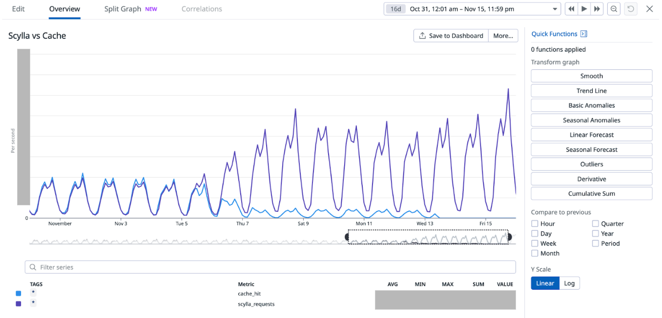
Scylla hit vs. cache hit
As we progressively disabled Redis cache for most of the counters, one obvious impact was the gradual increase in Scylla-bound QPS and similar decrease in Redis-cache hit. When Redis-cache was enabled for 100% of the configurations, 50% of the requests were bound for Scylla and the other 50% were for Redis. At the end of the experiment, after fully disabling Redis cache, 100% of the requests were Scylla-bound.

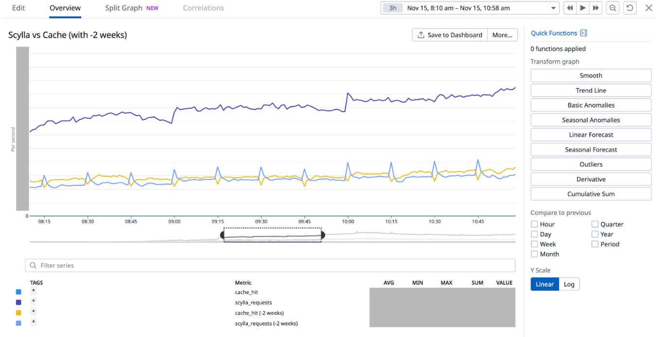
15-minutes and hourly spikes
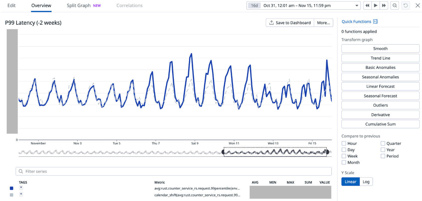
We noticed that the 15-minute spikes in Scylla QPS as well as the associated latency slowly became less prominent and eventually disappeared from the graph after we completely disabled the Redis cache. However, we noticed that the hourly spike still remained. This is attributed to the higher QPS from the clients calling this service at the turn of every hour. As a result, limited optimisation can be done to reduce the hourly spike on this service’s end.


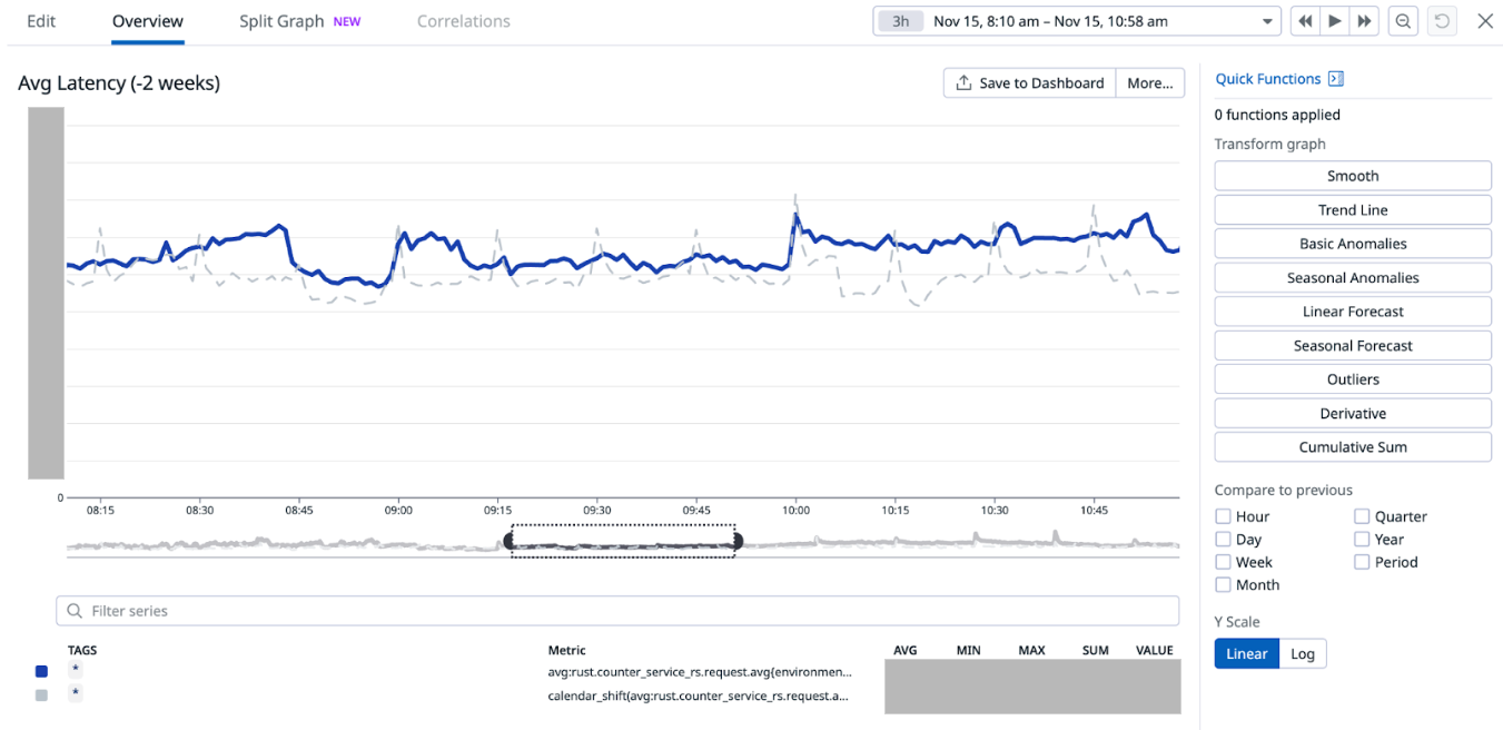
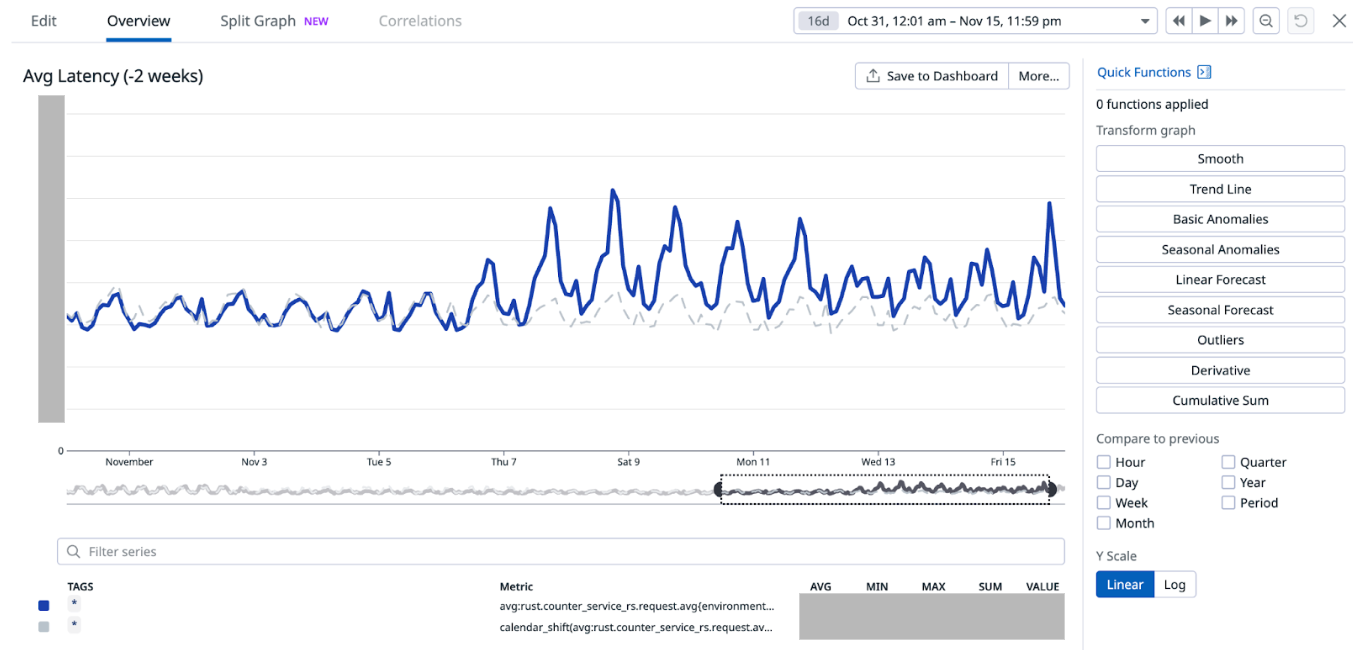
Service latency and additional Scylla compaction job
When we disabled Redis cache for about 75% of the counters configurations on Nov 7 (which accounts for about 85% of the overall QPS), we noticed an increase in the overall average service latency, from between 6-8 ms to 7-12 ms (P99 went from ~30-50ms to ~30-70ms). This caused a spike in open circuit breaker (CB) events on Hystrix. At this point, before disabling cache for more counters, on Nov 12, we experimented with running an additional major compaction job on Scylla between 2-5 PM on all our Scylla nodes, progressively on each availability zone (AZ). It is noteworthy that we already have a scheduled major compaction job that runs around 3 AM every day. The outcome of this experiment was quite positive. It brought back the average and P99 latency almost to the prior level when we had Redis cache enabled for 100% of the counters. This also had a similar effect on the Hystrix CB open events. Based on this observation, we made this additional day time major compaction job as a daily scheduled job. We disabled Redis cache for 100% of the counters the next day (Nov 13). This expectedly increased the Scylla QPS, with no noticeable adverse effect on the service latency or Hystrix CB open events.


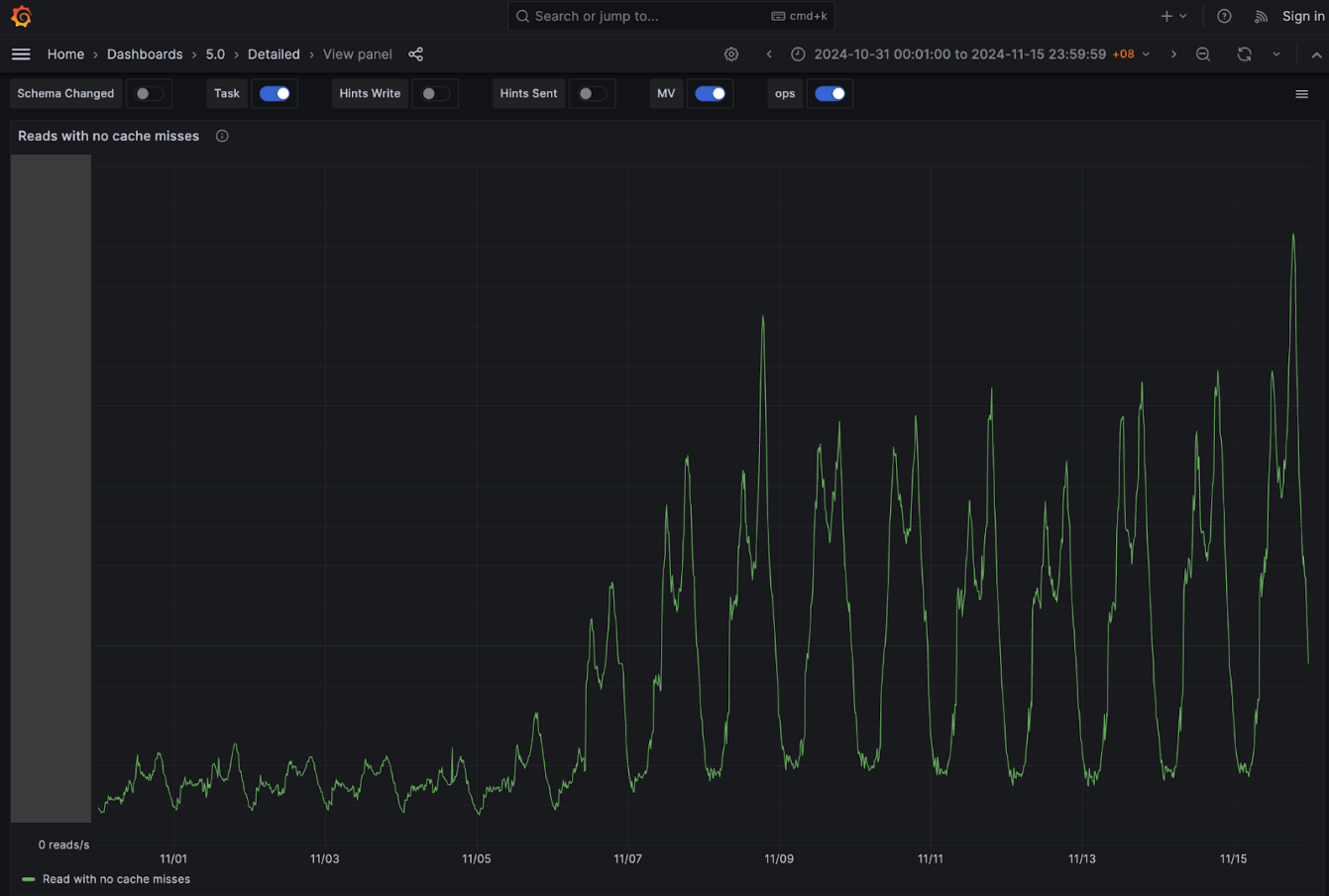
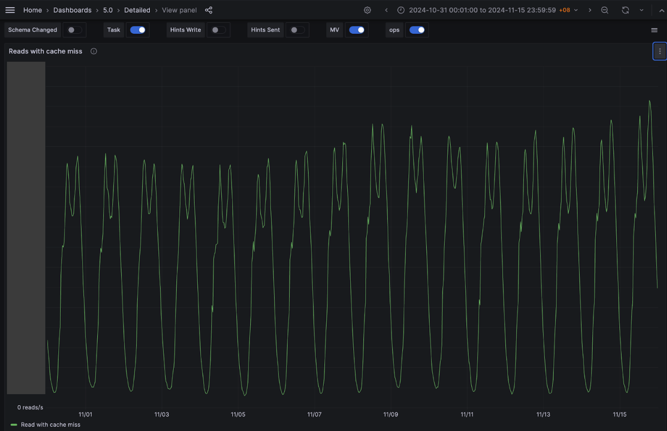
Scylla’s own cache
One of our hypotheses was that we were not using Scylla cache due to our system’s design, along with all the service specific characteristics discussed earlier. Our experimental results show that this is indeed the case. We observed a significant increase in Scylla reads with Scylla’s own cache hits, while Scylla reads with Scylla’s own cache misses remained about the same despite our Scylla cluster receiving double the traffic. Percentage-wise, before disabling the external Redis cache, Scylla hit its own cache for ~30% of the total reads, and after we have completely disabled the external Redis cache, Scylla hit its cache for about 70% of the reads. We believe that this largely contributes to the overall performance of the service despite fully decommissioning the expensive Redis cache component from our system architecture.


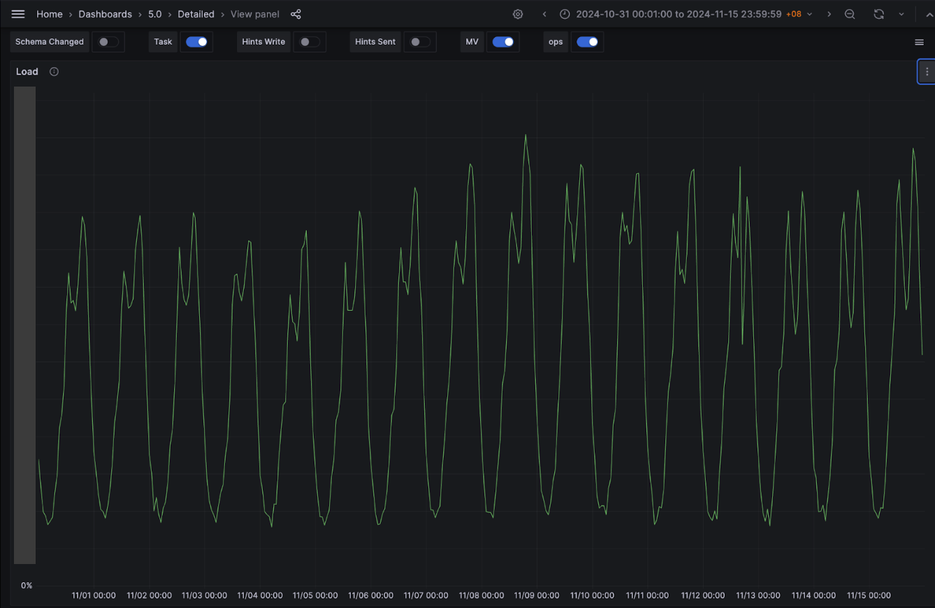
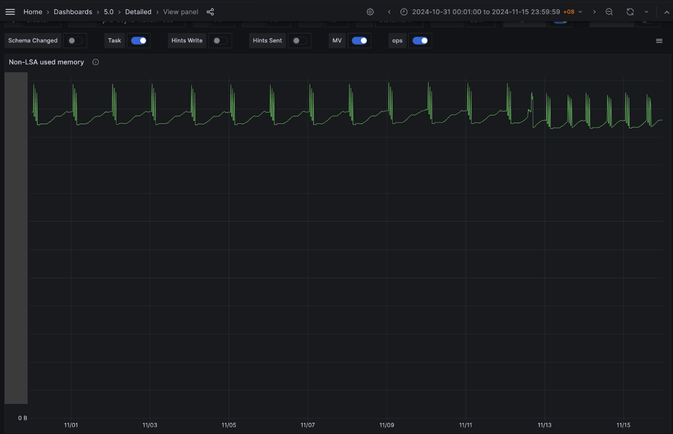
Scylla CPU and memory usage
Contrary to our assumption, although the Scylla QPS doubled due to the change done as part of this experiment, there was marginal increase in Scylla CPU usage (from ~50% to ~52% at peak). In terms of memory, Scylla log-structured allocator (LSA) memory usage remains consistent. For Non-LSA memory, the maximum utilisation did not increase. However, we noticed two daily spikes instead of one existed before the experiment. The second spike results from the newly added daily major compaction job. Notably,the overall non-LSA peak has slightly decreased after the introduction of the new compaction job.


Conclusion
In summary, we were able to maintain the same service performance while removing an expensive Redis cache component from our system architecture, which accounted for about 25% of the overall service cost. This has been made possible primarily by significant increase in the utilisation of Scylla’s own cache and adding a daily major compaction job on all our Scylla nodes.
In the future, we plan to further experiment with different Scylla configurations for potential performance gain, specifically to improve the latency.
Join us
Grab is a leading superapp in Southeast Asia, operating across the deliveries, mobility and digital financial services sectors. Serving over 800 cities in eight Southeast Asian countries, Grab enables millions of people everyday to order food or groceries, send packages, hail a ride or taxi, pay for online purchases or access services such as lending and insurance, all through a single app. Grab was founded in 2012 with the mission to drive Southeast Asia forward by creating economic empowerment for everyone. Grab strives to serve a triple bottom line – we aim to simultaneously deliver financial performance for our shareholders and have a positive social impact, which includes economic empowerment for millions of people in the region, while mitigating our environmental footprint.
Powered by technology and driven by heart, our mission is to drive Southeast Asia forward by creating economic empowerment for everyone. If this mission speaks to you, join our team today!