In today’s data-driven landscape, monitoring data quality has become a critical need for ensuring reliable and efficient data usage across domains. High-quality data is the backbone of AI innovation, driving efficiency and unlocking new opportunities. As decentralized data ownership grows, the ability to effectively monitor data quality is essential for maintaining reliability in data systems.
Kafka streams, as a vital component of real-time data processing, play a significant role in this ecosystem. However, unreliable data within Kafka streams can lead to errors and inefficiencies for downstream users, and monitoring the quality of data within these streams has always been a challenge. This blog introduces a solution that empowers stream users to define a data contract, specifying the rules that Kafka stream data must adhere to. By leveraging this user-defined data contract, the solution performs automated real-time data quality checks, identifies problematic data as it occurs, and promptly notifies stream owners. This ensures timely action, enabling effective monitoring and management of Kafka stream data quality while supporting the broader goals of data mesh and AI-driven innovation.
Problem statement
In the past, monitoring Kafka stream data processing lacked an effective solution for data quality validation. This limitation made it challenging to identify bad data, notify users in a timely manner, and prevent the cascading impact on downstream users from further escalating.
Challenges in syntactic and semantic issue identification:
Syntactic issues: Refers to schema mismatches between producers and consumers, which can lead to deserialization errors. While schema backward compatibility can be validated upon schema evolution, there are scenarios where the actual data in the Kafka topic does not align with the defined schema. For example, this can occur when a rogue Kafka producer is not using the expected schema for a given Kafka topic. Identifying the specific fields causing these syntactic issues is a typical challenge.
Semantic issues: Refers to inconsistencies or misalignments between producers and consumers about the expected pattern or significance of each field. Unlike Kafka stream schemas, which act as a data structure contract between producers and consumers, there is no existing framework for stakeholders to define and enforce field-level semantic rules, for example, the expected length or pattern of an identifier.
Timeliness challenge in data quality monitoring: There is no real-time mechanism to automatically validate data against predefined rules, timely identify quality issues, and promptly alert stream stakeholders. Without real-time stream validation, data quality issues can sometimes persist for periods of time, impacting various online and offline downstream systems before being discovered.
Observability challenge for troubleshooting bad data: Even when problematic data is identified, stream users face difficulties in pinpointing the exact “poison data” and understanding which fields are incompatible with the schema or violate semantic rules. This lack of visibility complicates Root Cause Analysis and resolution efforts.
Solution
Our Coban platform offers a standardized data quality test and observability solution at the platform level, consisting of the following components:
Data Contract Definition: Enables Kafka stream stakeholders to define contracts that include schema agreements, semantic rules that Kafka topic data must comply with, and Kafka stream ownership details for alerting and notifications.
Automated Test Execution: Provides a long running Test Runner to automatically execute real-time tests based on the defined contract.
Real-time Data Quality Issue Identification: Detects data issues at both syntactic and semantic levels in real-time.
Alerts and Result Observability: Alerts users, simplifying observation of data quality issues via the platform.
Architecture details
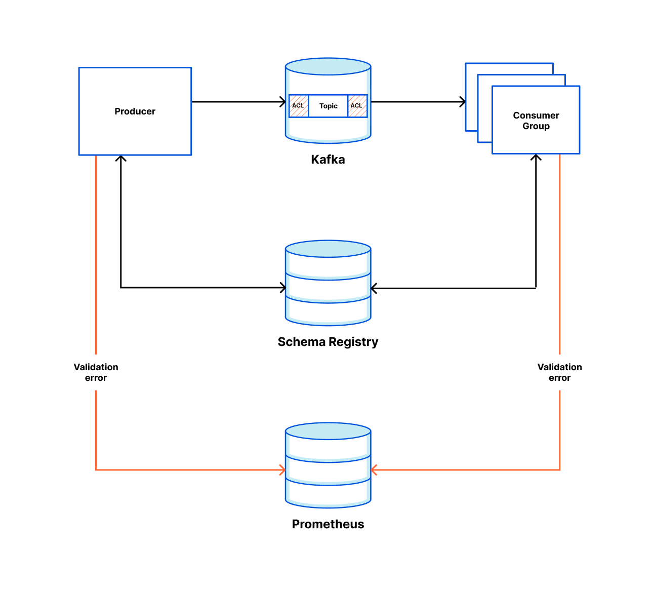
The solution includes three components: Data Contract Definition, Test Execution & Data Quality Issue Identification, and Result Observability as shown in the architecture diagram in figure 1. All mentions of “Flow” from here onwards refer to the corresponding processes illustrated in figure 1.
Figure 1. Real-time Kafka Stream Data Quality Monitoring Architecture diagram.
Data Contract Definition
The Coban Platform streamlines the process of defining Kafka stream data contracts, serving as a formal agreement among Kafka stream stakeholders. This includes the following components:
Kafka Stream Schema: Represents the schema used by the Kafka topic under test and helps the Test Runner to validate schema compatibility across data streams (Flow 1.1).
Kafka Stream Configuration: Encompasses essential configurations such as the endpoint and topic name, which the platform automatically populates (Flow 1.2).
Observability Metadata: Provides contact information for notifying Kafka stream stakeholders about data quality issues and includes alert configurations for monitoring (Flow 1.3).
Kafka Stream Semantic Test Rules: Empowers users to define intuitive semantic test rules at the field level. These rules include checks for string patterns, number ranges, constant values, etc. (Flow 1.5).
LLM-Based Semantic Test Rules Recommendation: Defining dozens if not hundreds of field-specific test rules can overwhelm users. To simplify this process, the Coban Platform uses LLM-based recommendations to predict semantic test rules using provided Kafka stream schemas and anonymized sample data (Flow 1.4). This feature helps users set up semantic rules efficiently, as demonstrated in the sample UI in figure 2.
Figure 2. Sample UI showcasing LLM-based Kafka stream schema field-level semantic test rules. Note that the data shown is entirely fictional.
Data Contract Transformation
Once defined, the Coban Platform’s transformation engine converts the data contract into configurations that the Test Runner can interpret (Flow 2.1). This transformation process includes:
Kafka Stream Schema: Translates the schema defined in the data contract into a schema reference that the Test Runner can parse.
Kafka Stream Configuration: Sets up the Kafka stream as a source for the Test Runner.
Observability metadata: Sets contact information as configurations of the Test Runner.
Kafka Stream Semantic Test Rules: Transforms human-readable semantic test rules into an inverse SQL query to capture the data that violates the defined rules.
Figure 3. Illustration of semantic test rules being converted from human-readable formats into inverse SQL queries.
Test Execution & Data Quality Issue Identification
Once the Test Configuration Transformation Engine generates the Test Runner configuration (Flow 2.1), the platform automatically deploys the Test Runner.
Test Runner
The Test Runner utilises FlinkSQL as the compute engine to execute the tests. FlinkSQL was selected for its flexibility in defining test rules as straightforward SQL statements, enabling our platform to efficiently convert data contracts into enforceable rules.
Test Execution Workflow And Problematic Data Identification
FlinkSQL consumes data from the Kafka topic under test (Flow 2.2) using its own consumer group, ensuring it doesn’t impact other consumers. It runs the inverse SQL query (Flow 2.3) to identify any data that violates the semantic rules or that is syntactically incorrect in the first place. Test Runner captures such data, packages it into a data quality issue event enriched with a test summary, the total count of bad records, and sample bad data, and publishes it to a dedicated Kafka topic (Flow 3.2). Additionally, the platform sinks all such data quality events to an AWS S3 bucket (Flow 3.1) to enable deeper observability and analysis.
Result Observability
Grab’s in-house data quality observability platform, Genchi, consumes problematic data captured by the Test Runner (Flow 3.3).
Alerting
Genchi sends Slack notifications (Flow 3.5) to stream owners specified in the data contract observability metadata. These notifications include detailed information about stream issues, such as links to sample data in Coban UI, observed windows, counts of bad records, and other relevant details.
Figure 4. Sample Slack notifications
Observability
Users can access the Coban UI (Flow 3.4), displaying Kafka stream test rules and sample bad records, highlighting fields and values that violate rules.
Figure 5. In this Sample Test Result, the highlighted fields indicate violations of the semantic test rules.
Impact
Since its deployment earlier this year, the solution has enabled Kafka stream users to define contracts with syntactic and semantic rules, automate test execution, and alert users when problematic data is detected, prompting timely action. It has been actively monitoring data quality across 100+ critical Kafka topics. The solution offers the capability to immediately identify and halt the propagation of invalid data across multiple streams.
Conclusion
We implemented and rolled out a solution to assist Grab engineers in effectively monitoring data quality in their Kafka streams. This solution empowers them to establish syntactic and semantic tests for their data. Our platform’s automatic testing feature enables real-time tracking of data quality, with instant alerts for any discrepancies. Additionally, we provide detailed visibility into test results, facilitating the easy identification of specific data fields that violate the rules. This accelerates the process of diagnosing and resolving issues, allowing users to swiftly address production data challenges.
What’s next
While our current solution emphasizes monitoring the quality of Kafka streaming data, further exploration will focus on tracing producers to pinpoint the origin of problematic data, as well as enabling more advanced semantic tests such as cross-field validations. Additionally, we aim to expand monitoring capabilities to cover broader aspects like data completeness and freshness, and integrate with Gable AI to detect Data Transfer Object (DTO) changes and semantic regressions in Go producers upon committing code to the Git repository. These enhancements will pave the way for a more robust, multidimensional data quality testing solution across a wider range.
Grab is a leading superapp in Southeast Asia, operating across the deliveries, mobility and digital financial services sectors. Serving over 800 cities in eight Southeast Asian countries, Grab enables millions of people everyday to order food or groceries, send packages, hail a ride or taxi, pay for online purchases or access services such as lending and insurance, all through a single app. Grab was founded in 2012 with the mission to drive Southeast Asia forward by creating economic empowerment for everyone. Grab strives to serve a triple bottom line – we aim to simultaneously deliver financial performance for our shareholders and have a positive social impact, which includes economic empowerment for millions of people in the region, while mitigating our environmental footprint.
Powered by technology and driven by heart, our mission is to drive Southeast Asia forward by creating economic empowerment for everyone. If this mission speaks to you, join our team today!
Tudum.com is Netflix’s official fan destination, enabling fans to dive deeper into their favorite Netflix shows and movies. Tudum offers exclusive first-looks, behind-the-scenes content, talent interviews, live events, guides, and interactive experiences. “Tudum” is named after the sonic ID you hear when pressing play on a Netflix show or movie. Attracting over 20 million members each month, Tudum is designed to enrich the viewing experience by offering additional context and insights into the content available on Netflix.
Initial architecture
At the end of 2021, when we envisioned Tudum’s implementation, we considered architectural patterns that would be maintainable, extensible, and well-understood by engineers. With the goal of building a flexible, configuration-driven system, we looked to server-driven UI (SDUI) as an appealing solution. SDUI is a design approach where the server dictates the structure and content of the UI, allowing for dynamic updates and customization without requiring changes to the client application. Client applications like web, mobile, and TV devices, act as rendering engines for SDUI data. After our teams weighed and vetted all the details, the dust settled and we landed on an approach similar to Command Query Responsibility Segregation (CQRS). At Tudum, we have two main use cases that CQRS is perfectly capable of solving:
Tudum’s editorial team brings exclusive interviews, first-look photos, behind the scenes videos, and many more forms of fan-forward content, and compiles it all into pages on the Tudum.com website. This content comes onto Tudum in the form of individually published pages, and content elements within the pages. In support of this, Tudum’s architecture includes a write path to store all of this data, including internal comments, revisions, version history, asset metadata, and scheduling settings.
Tudum visitors consume published pages. In this case, Tudum needs to serve personalized experiences for our beloved fans, and accesses only the latest version of our content.
Initial Tudum data architecture
The high-level diagram above focuses on storage & distribution, illustrating how we leveraged Kafka to separate the write and read databases. The write database would store internal page content and metadata from our CMS. The read database would store read-optimized page content, for example: CDN image URLs rather than internal asset IDs, and movie titles, synopses, and actor names instead of placeholders. This content ingestion pipeline allowed us to regenerate all consumer-facing content on demand, applying new structure and data, such as global navigation or branding changes. The Tudum Ingestion Service converted internal CMS data into a read-optimized format by applying page templates, running validations, performing data transformations, and producing the individual content elements into a Kafka topic. The Data Service Consumer, received the content elements from Kafka, stored them in a high-availability database (Cassandra), and acted as an API layer for the Page Construction service and other internal Tudum services to retrieve content.
A key advantage of decoupling read and write paths is the ability to scale them independently. It is a well-known architectural approach to connect both write and read databases using an event driven architecture. As a result, content edits would eventually appear on tudum.com.
Challenges with eventual consistency
Did you notice the emphasis on “eventually?” A major downside of this architecture was the delay between making an edit and observing that edit reflected on the website. For instance, when the team publishes an update, the following steps must occur:
Call the REST endpoint on the 3rd party CMS to save the data.
Wait for the CMS to notify the Tudum Ingestion layer via a webhook.
Wait for the Tudum Ingestion layer to query all necessary sections via API, validate data and assets, process the page, and produce the modified content to Kafka.
Wait for the Data Service Consumer to consume this message from Kafka and store it in the database.
Finally, after some cache refresh delay, this data would eventually become available to the Page Construction service. Great!
By introducing a highly-scalable eventually-consistent architecture we were missing the ability to quickly render changes after writing them — an important capability for internal previews.
In our performance profiling, we found the source of delay was our Page Data Service which acted as a facade for an underlying Key Value Data Abstraction database. Page Data Service utilized a near cache to accelerate page building and reduce read latencies from the database.
This cache was implemented to optimize the N+1 key lookups necessary for page construction by having a complete data set in memory. When engineers hear “slow reads,” the immediate answer is often “cache,” which is exactly what our team adopted. The KVDAL near cache can refresh in the background on every app node. Regardless of which system modifies the data, the cache is updated with each refresh cycle. If you have 60 keys and a refresh interval of 60 seconds, the near cache will update one key per second. This was problematic for previewing recent modifications, as these changes were only reflected with each cache refresh. As Tudum’s content grew, cache refresh times increased, further extending the delay.
RAW Hollow
As this pain point grew, a new technology was being developed that would act as our silver bullet. RAW Hollow is an innovative in-memory, co-located, compressed object database developed by Netflix, designed to handle small to medium datasets with support for strong read-after-write consistency. It addresses the challenges of achieving consistent performance with low latency and high availability in applications that deal with less frequently changing datasets. Unlike traditional SQL databases or fully in-memory solutions, RAW Hollow offers a unique approach where the entire dataset is distributed across the application cluster and resides in the memory of each application process.
This design leverages compression techniques to scale datasets up to 100 million records per entity, ensuring extremely low latencies and high availability. RAW Hollow provides eventual consistency by default, with the option for strong consistency at the individual request level, allowing users to balance between high availability and data consistency. It simplifies the development of highly available and scalable stateful applications by eliminating the complexities of cache synchronization and external dependencies. This makes RAW Hollow a robust solution for efficiently managing datasets in environments like Netflix’s streaming services, where high performance and reliability are paramount.
Revised architecture
Tudum was a perfect fit to battle-test RAW Hollow while it was pre-GA internally. Hollow’s high-density near cache significantly reduces I/O. Having our primary dataset in memory enables Tudum’s various microservices (page construction, search, personalization) to access data synchronously in O(1) time, simplifying architecture, reducing code complexity, and increasing fault tolerance.
Updated Tudum data architecture
In our simplified architecture, we eliminated the Page Data Service, Key Value store, and Kafka infrastructure, in favor of RAW Hollow. By embedding the in-memory client directly into our read-path services, we avoid per-request I/O and reduce roundtrip time.
Migration results
The updated architecture yielded a monumental reduction in data propagation times, and the reduced I/O led to faster request times as an added bonus. Hollow’s compression alleviated our concerns about our data being “too big” to fit in memory. Storing three years’ of unhydrated data requires only a 130MB memory footprint — 25% of its uncompressed size in an Iceberg table!
Writers and editors can preview changes in seconds instead of minutes, while still maintaining high-availability and in-memory caching for Tudum visitors — the best of both worlds.
But what about the faster request times? The diagram below illustrates the before & after timing to fulfil a request for Tudum’s home page. All of Tudum’s read-path services leverage Hollow in-memory state, leading to a significant increase in page construction speed and personalization algorithms. Controlling for factors like TLS, authentication, request logging, and WAF filtering, homepage construction time decreased from ~1.4 seconds to ~0.4 seconds!
Home page construction time
An attentive reader might notice that we have now tightly-coupled our Page Construction Service with the Hollow In-Memory State. This tight-coupling is used only in Tudum-specific applications. However, caution is needed if sharing the Hollow In-Memory Client with other engineering teams, as it could limit your ability to make schema changes or deprecations.
Key Learnings
CQRS is a powerful design paradigm for scale, if you can tolerate some eventual consistency.
Minimizing the number of sequential operations can significantly reduce response times. I/O is often the main enemy of performance.
Caching is complicated. Cache invalidation is a hard problem. By holding an entire dataset in memory, you can eliminate an entire class of problems.
In the next episode, we’ll share how Tudum.com leverages Server Driven UI to rapidly build and deploy new experiences for Netflix fans. Stay tuned!
As organizations build modern applications with event-driven architectures (EDA), they often seek solutions that minimize infrastructure management overhead while maximizing developer productivity. Amazon Managed Streaming for Apache Kafka (Amazon MSK) and AWS Lambda together provide a serverless, scalable, and cost-efficient platform for real-time event-driven processing.
In this post, we describe how you can simplify your event-driven application architecture using AWS Lambda with Amazon MSK. We demonstrate how to configure Lambda as a consumer for Kafka topics, including a cross-account setup and how to optimize price and performance for these applications.
Why use Lambda with Amazon MSK?
Customers building event-driven applications have several key priorities when it comes to their architecture choices. They typically seek to reduce their operational overhead by using Amazon Web Services (AWS) to handle the complex, underlying infrastructure components so their teams can focus on core business logic. Additionally, developers prefer a streamlined experience that minimizes the need for repetitive boilerplate code, enabling them to be more productive and focus on creating value. Furthermore, these customers want to achieve both scalability and cost-effectiveness without the burden of managing compute infrastructure directly. Lambda integration with Amazon MSK effectively addresses these requirements, delivering a comprehensive solution that combines the benefits of serverless computing with managed Kafka services. For example, an ecommerce company can use Amazon MSK to collect real-time clickstream data from its website and process those events using AWS Lambda. With this integration, they can trigger Lambda functions to update recommendation models, send personalized offers, or analyze user behavior instantly—without provisioning or managing servers. The key benefits of using Lambda with Amazon MSK include:
Simplicity through native integration – AWS Lambda offers native integration with Amazon MSK through a connector resource called event source mapping. You can use this integration to directly associate a Kafka topic—whether it’s on Amazon MSK or a self-managed Kafka cluster—as an event source for a Lambda function without writing custom consumer logic. With just a few configuration steps, event source mapping handles partition assignment, offset tracking, and parallelized batch processing under the hood. It uses the Kafka consumer group protocol to distribute topic partitions across multiple concurrent Lambda invocations, supports batch windowing, and enables at-least-once delivery semantics. Moreover, it automatically commits offsets upon successful function execution while handling retries and dead-letter queue (DLQ) routing for failed records, significantly reducing the operational overhead traditionally associated with Kafka consumers.
Auto scaling and throughput controls – When using AWS Lambda with Amazon MSK through event source mapping, Lambda automatically scales by assigning a dedicated event poller per Kafka partition, enabling parallel, partition-based processing. This allows the system to elastically handle varying traffic without manual intervention. For advanced control, provisioned concurrency pre-initializes Lambda execution environments, eliminating cold starts and delivering consistent low-latency performance. Additionally, with provisioned event source mapping, you can configure the minimum and maximum number of Kafka pollers, providing precise control over throughput and concurrency. This is ideal for applications with unpredictable traffic patterns or strict latency requirements.
Cost-effectiveness – AWS Lambda uses a pay-per-use model in which you only pay for compute time and number of invocations. When integrated with Amazon MSK, there are no charges for idle time, making it ideal for bursty or low-frequency Kafka workloads. You can further optimize costs by tuning batch size and batch window settings. For mission-critical workloads, provisioned concurrency provides consistent performance with controlled pricing.
Event filtering – AWS Lambda supports event filtering for Amazon MSK event sources, which means you can process only the Kafka records that match specific criteria. This reduces unnecessary function invocations and optimizes your function costs. You can define up to five filters per event source mapping (with the option to request an increase to ten). Each filter uses a JSON-based pattern to specify the conditions a record must meet to be processed. Filters can be applied using the AWS Management Console, AWS Command Line Interface (AWS CLI), or AWS Serverless Application Model (AWS SAM) templates. For more details and examples, refer to the AWS Lambda documentation on event filtering with Amazon MSK.
Handling Availability Zone outage for your consumer – Amazon MSK enables high availability for your Kafka brokers by distributing them across multiple Availability Zones within a Region. To maintain high availability across your application, you similarly need a consumer that offers high availability. AWS Lambda offers high availability and resilience by running your consumer functions across multiple Availability Zones in a Region. This means that even if one Availability Zone experiences an outage, your Lambda function will continue to operate in other healthy Availability Zones. While Lambda manages security patching and Availability Zone failure scenarios, you can focus on your application logic.
Cross-account event processing – Cross-account connectivity between AWS Lambda and Amazon MSK allows a Lambda function in one AWS account to consume data from an MSK cluster in another account using MSK multi-VPC private connectivity powered by AWS PrivateLink. This setup is particularly beneficial for organizations that centralize Kafka infrastructure while maintaining separate accounts for different applications or teams.
Support for JSON, Avro, Protobuf, and Schema Registries – AWS Lambda supports Kafka events in JSON, Avro and Protobuf formats via event source mapping. It integrates with AWS Glue Schema registry, Confluent Cloud Schema registry, and self-managed Confluent Schema registry , enabling native schema validation, filtering, and deserialization without custom code.
How Lambda processes messages from your Kafka topic
Lambda uses event source mappings to process records from Amazon MSK by actively polling Kafka topics through event pollers that invoke Lambda functions with batches of records. These mappings are Lambda managed resources designed for high-throughput, stream-based processing. By default, Lambda detects the OffsetLag for all partitions in your Kafka topic and automatically scales pollers based on traffic. For high-throughput applications, you can enable provisioned mode to define minimum and maximum pollers, and your event source mapping auto scales between the minimum and maximum defined values. In the provisioned mode, each poller can process up to 5 MBps and supports concurrent Lambda invocations.
After Lambda processes each batch, it commits the offsets of the messages in that batch. If your function returns an error for a message in a batch, Lambda retries the whole batch of messages until processing succeeds or the messages expire. You can send records that fail all retry attempts to an on-failure destination for later processing. To maintain ordered processing within a partition, Lambda limits the maximum event pollers to the number of partitions in the topic. When setting up Kafka as a Lambda event source, you can specify a consumer group ID to let Lambda join an existing Kafka consumer group. If other consumers are active in that group, Lambda will receive only part of the topic’s messages. If the group exists, Lambda starts from the group’s committed offset, ignoring the StartingPosition. The following diagram illustrates this flow.
Walkthrough: Build a serverless Kafka app with AWS Lambda
Follow these steps to build a serverless application that consumes messages from an MSK cluster using AWS Lambda:
Create an Amazon MSK cluster. Use the AWS Management Console or AWS CLI to create your MSK cluster. When the cluster is up, create your Kafka topic(s). For detailed instructions, refer to the Amazon MSK documentation.
Create a Lambda function using the AWS Management Console or the AWS CLI. To learn more about creating a Lambda function, refer to Create your first Lambda function. The Lambda function’s execution role needs to have the following permissions:
Access to connect to your MSK cluster
Permissions to manage elastic network interfaces in your VPC
To connect Lambda to Amazon MSK as a consumer, set up event source mapping to link your MSK topic with the Lambda function. This allows Lambda to automatically poll for new messages and process them. Follow the guide on how to configure event source mapping.
For reference, configuring event source mapping involves three steps:
Network setup – In the default event source mapping mode, you need to configure a networking setup using a PrivateLink endpoint or NAT gateway for event source mapping to invoke Lambda functions. In provisioned mode, no networking configuration is needed (and you don’t incur the cost of networking components).
Event source mapping parameter configuration – This involves setting necessary configuration parameters for the event source mapping to be able to poll messages from your Kafka cluster. This includes the MSK cluster, topic name, consumer group ID, authentication method, and optionally, schema registry, scaling mode. You can configure the scaling mode for provisioned throughput, along with batch size, batch window, and event filtering for your event source mapping.
Access permissions – This involves configuring required permissions to access the required AWS resources, and includes configuring permissions for the function to execute the code, permissions for the event source mapping to access your MSK cluster, and permissions for Lambda to access your VPC resources.
The following screenshot shows the console setup for configuring Amazon MSK event source mapping, including the Amazon MSK trigger related fields.
The following screenshot shows event poller configuration.
The following screenshot shows additional settings you can use, depending on your use case.
Optimizing AWS Lambda for stream processing with Amazon MSK
When building real-time data processing pipelines with Amazon MSK and AWS Lambda, it’s important to tune your setup for both performance and cost-efficiency. Lambda offers powerful serverless compute capabilities, but to get the most out of it in a streaming context, you need to make a few key optimizations:
Enable provisioned concurrency for low-latency processing – For workloads that are sensitive to latency—cold starts can introduce unwanted delays. By enabling provisioned concurrency, you can pre-warm a specified number of Lambda instances so they’re always ready to handle traffic immediately. This eliminates cold starts and provides consistent response times, which is crucial for latency-critical use cases.
Enable provisioned mode for event source mapping for high-throughput processing – For Kafka workloads with stringent throughput requirements, activate the provisioned mode. The optimal configuration of minimum and maximum event pollers for your Kafka event source mapping depends on your application’s performance requirements. Start with the default minimum event pollers to baseline the performance profile and adjust event pollers based on observed message processing patterns and your application’s performance requirements. For workloads with spiky traffic and strict performance needs, increase the minimum event pollers to handle sudden surges. You can fine-tune the minimum event pollers by evaluating your desired throughput, your observed throughput, which depends on factors such as the ingested messages per second and average payload size, and using the throughput capacity of one event poller (up to 5 MB/s) as reference. To maintain ordered processing within a partition, Lambda caps the maximum event pollers at the number of partitions in the topic.
Optimize message batching using size and windowing – By integrating Lambda with Amazon MSK, you can control how messages are batched before they’re sent to your function. Tuning parameters such as batch size (the number of records per invocation: 1–10,000 records) and maximum batching window (how long to wait for a full batch: 0–300 seconds) can significantly impact performance. Larger batches mean fewer invocations, which reduces overhead and improves throughput. However, it’s important to strike a balance—too large a batch or window might introduce unwanted processing delays. Monitor your stream’s behavior and adjust these settings based on throughput requirements and acceptable latency.
Apply filters to reduce unnecessary invocations – Not every record in your Kafka topic might require processing. To avoid unnecessary Lambda invocations (and associated costs), apply filtering logic directly when configuring the event source mapping. With Lambda, you can define filtering (up to 10 filters) criteria so that only relevant records trigger your function. This helps reduce compute time, minimize noise, and optimize your budget, especially when dealing with high-throughput topics with mixed content. For Amazon MSK, Lambda commits offsets for matched and unmatched messages after successfully invoking the function.
Conclusion
By combining Amazon MSK with AWS Lambda, you can seamlessly build modern, serverless event-driven applications. This integration eliminates the need to manage consumer groups, compute infrastructure, or scaling logic so teams can focus on delivering business value faster.
Whether you’re integrating Kafka into microservices, transforming data pipelines, or building reactive applications, Lambda with Amazon MSK is a powerful and flexible serverless solution. For detailed documentation on how to configure Lambda with Amazon MSK, refer to the AWS Lambda Developer Guide. For more serverless learning resources, visit Serverless Land.
About the Authors
Tarun Rai Madan is a Principal Product Manager at Amazon Web Services (AWS). He specializes in serverless technologies and leads product strategy to help customers achieve accelerated business outcomes with event-driven applications, using services like AWS Lambda, AWS Step Functions, Apache Kafka, and Amazon SQS/SNS. Prior to AWS, he was an engineering leader in the semiconductor industry, and led development of high-performance processors for wireless, automotive, and data center applications.
Masudur Rahaman Sayem is a Streaming Data Architect at AWS with over 25 years of experience in the IT industry. He collaborates with AWS customers worldwide to architect and implement sophisticated data streaming solutions that address complex business challenges. As an expert in distributed computing, Sayem specializes in designing large-scale distributed systems architecture for maximum performance and scalability. He has a keen interest and passion for distributed architecture, which he applies to designing enterprise-grade solutions at internet scale.
According to a survey done by W3Techs, as of October 2024, Cloudflare is used as an authoritative DNS provider by 14.5% of all websites. As an authoritative DNS provider, we are responsible for managing and serving all the DNS records for our clients’ domains. This means we have an enormous responsibility to provide the best service possible, starting at the data plane. As such, we are constantly investing in our infrastructure to ensure the reliability and performance of our systems.
DNS is often referred to as the phone book of the Internet, and is a key component of the Internet. If you have ever used a phone book, you know that they can become extremely large depending on the size of the physical area it covers. A zone file in DNS is no different from a phone book. It has a list of records that provide details about a domain, usually including critical information like what IP address(es) each hostname is associated with. For example:
example.com      59 IN A 198.51.100.0
blog.example.com 59 IN A 198.51.100.1
ask.example.com  59 IN A 198.51.100.2
It is not unusual for these zone files to reach millions of records in size, just for a single domain. The biggest single zone on Cloudflare holds roughly 4 million DNS records, but the vast majority of zones hold fewer than 100 DNS records. Given our scale according to W3Techs, you can imagine how much DNS data alone Cloudflare is responsible for. Given this volume of data, and all the complexities that come at that scale, there needs to be a very good reason to move it from one database cluster to another.
Why migrate
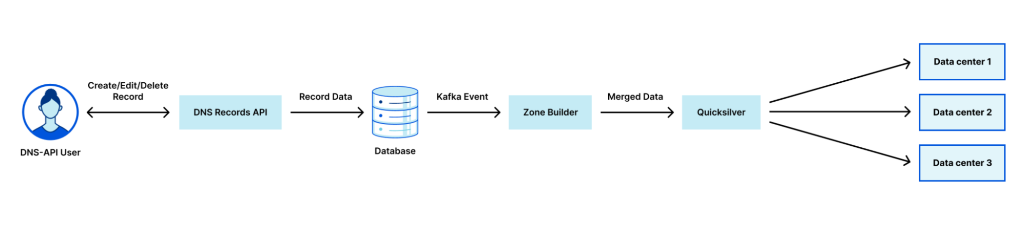
When initially measured in 2022, DNS data took up approximately 40% of the storage capacity in Cloudflare’s main database cluster (cfdb). This database cluster, consisting of a primary system and multiple replicas, is responsible for storing DNS zones, propagated to our data centers in over 330 cities via our distributed KV store Quicksilver. cfdb is accessed by most of Cloudflare’s APIs, including the DNS Records API. Today, the DNS Records API is the API most used by our customers, with each request resulting in a query to the database. As such, it’s always been important to optimize the DNS Records API and its surrounding infrastructure to ensure we can successfully serve every request that comes in.
As Cloudflare scaled, cfdb was becoming increasingly strained under the pressures of several services, many unrelated to DNS. During spikes of requests to our DNS systems, other Cloudflare services experienced degradation in the database performance. It was understood that in order to properly scale, we needed to optimize our database access and improve the systems that interact with it. However, it was evident that system level improvements could only be just so useful, and the growing pains were becoming unbearable. In late 2022, the DNS team decided, along with the help of 25 other teams, to detach itself from cfdb and move our DNS records data to another database cluster.
Pre-migration
From a DNS perspective, this migration to an improved database cluster was in the works for several years. Cloudflare initially relied on a single Postgres database cluster, cfdb. At Cloudflare’s inception, cfdb was responsible for storing information about zones and accounts and the majority of services on the Cloudflare control plane depended on it. Since around 2017, as Cloudflare grew, many services moved their data out of cfdb to be served by a microservice. Unfortunately, the difficulty of these migrations are directly proportional to the amount of services that depend on the data being migrated, and in this case, most services require knowledge of both zones and DNS records.
Although the term “zone” was born from the DNS point of view, it has since evolved into something more. Today, zones on Cloudflare store many different types of non-DNS related settings and help link several non-DNS related products to customers’ websites. Therefore, it didn’t make sense to move both zone data and DNS record data together. This separation of two historically tightly coupled DNS concepts proved to be an incredibly challenging problem, involving many engineers and systems. In addition, it was clear that if we were going to dedicate the resources to solving this problem, we should also remove some of the legacy issues that came along with the original solution.
One of the main issues with the legacy database was that the DNS team had little control over which systems accessed exactly what data and at what rate. Moving to a new database gave us the opportunity to create a more tightly controlled interface to the DNS data. This was manifested as an internal DNS Records gRPC API which allows us to make sweeping changes to our data while only requiring a single change to the API, rather than coordinating with other systems. For example, the DNS team can alter access logic and auditing procedures under the hood. In addition, it allows us to appropriately rate-limit and cache data depending on our needs. The move to this new API itself was no small feat, and with the help of several teams, we managed to migrate over 20 services, using 5 different programming languages, from direct database access to using our managed gRPC API. Many of these services touch very important areas such as DNSSEC, TLS, Email, Tunnels, Workers, Spectrum, and R2 storage. Therefore, it was important to get it right.
One of the last issues to tackle was the logical decoupling of common DNS database functions from zone data. Many of these functions expect to be able to access both DNS record data and DNS zone data at the same time. For example, at record creation time, our API needs to check that the zone is not over its maximum record allowance. Originally this check occurred at the SQL level by verifying that the record count was lower than the record limit for the zone. However, once you remove access to the zone itself, you are no longer able to confirm this. Our DNS Records API also made use of SQL functions to audit record changes, which requires access to both DNS record and zone data. Luckily, over the past several years, we have migrated this functionality out of our monolithic API and into separate microservices. This allowed us to move the auditing and zone setting logic to the application level rather than the database level. Ultimately, we are still taking advantage of SQL functions in the new database cluster, but they are fully independent of any other legacy systems, and are able to take advantage of the latest Postgres version.
Now that Cloudflare DNS was mostly decoupled from the zones database, it was time to proceed with the data migration. For this, we built what would become our Change Data Capture and Transfer Service (CDCTS).
Requirements for the Change Data Capture and Transfer Service
The Database team is responsible for all Postgres clusters within Cloudflare, and were tasked with executing the data migration of two tables that store DNS data: cf_rec and cf_archived_rec, from the original cfdb cluster to a new cluster we called dnsdb. We had several key requirements that drove our design:
Don’t lose data. This is the number one priority when handling any sort of data. Losing data means losing trust, and it is incredibly difficult to regain that trust once it’s lost. Important in this is the ability to prove no data had been lost. The migration process would, ideally, be easily auditable.
Minimize downtime. We wanted a solution with less than a minute of downtime during the migration, and ideally with just a few seconds of delay.
These two requirements meant that we had to be able to migrate data changes in near real-time, meaning we either needed to implement logical replication, or some custom method to capture changes, migrate them, and apply them in a table in a separate Postgres cluster.
We first looked at using Postgres logical replication using pgLogical, but had concerns about its performance and our ability to audit its correctness. Then some additional requirements emerged that made a pgLogical implementation of logical replication impossible:
The ability to move data must be bidirectional. We had to have the ability to switch back to cfdb without significant downtime in case of unforeseen problems with the new implementation.
Partition the cf_rec table in the new database. This was a long-desired improvement and since most access to cf_rec is by zone_id, it was decided that mod(zone_id, num_partitions) would be the partition key.
Transferred data accessible from original database. In case we had functionality that still needed access to data, a foreign table pointing to dnsdb would be available in cfdb. This could be used as emergency access to avoid needing to roll back the entire migration for a single missed process.
Only allow writes in one database. Applications should know where the primary database is, and should be blocked from writing to both databases at the same time.
Details about the tables being migrated
The primary table, cf_rec, stores DNS record information, and its rows are regularly inserted, updated, and deleted. At the time of the migration, this table had 1.7 billion records, and with several indexes took up 1.5 TB of disk. Typical daily usage would observe 3-5 million inserts, 1 million updates, and 3-5 million deletes.
The second table, cf_archived_rec, stores copies of cf_rec that are obsolete — this table generally only has records inserted and is never updated or deleted. As such, it would see roughly 3-5 million inserts per day, corresponding to the records deleted from cf_rec. At the time of the migration, this table had roughly 4.3 billion records.
Fortunately, neither table made use of database triggers or foreign keys, which meant that we could insert/update/delete records in this table without triggering changes or worrying about dependencies on other tables.
Ultimately, both of these tables are highly active and are the source of truth for many highly critical systems at Cloudflare.
Designing the Change Data Capture and Transfer Service
There were two main parts to this database migration:
Initial copy: Take all the data from cfdb and put it in dnsdb.
Change copy: Take all the changes in cfdb since the initial copy and update dnsdb to reflect them. This is the more involved part of the process.
Normally, logical replication replays every insert, update, and delete on a copy of the data in the same transaction order, making a single-threaded pipeline. We considered using a queue-based system but again, speed and auditability were both concerns as any queue would typically replay one change at a time. We wanted to be able to apply large sets of changes, so that after an initial dump and restore, we could quickly catch up with the changed data. For the rest of the blog, we will only speak about cf_rec for simplicity, but the process for cf_archived_rec is the same.
What we decided on was a simple change capture table. Rows from this capture table would be loaded in real-time by a database trigger, with a transfer service that could migrate and apply thousands of changed records to dnsdb in each batch. Lastly, we added some auditing logic on top to ensure that we could easily verify that all data was safely transferred without downtime.
Basic model of change data capture
For cf_rec to be migrated, we would create a change logging table, along with a trigger function and a table trigger to capture the new state of the record after any insert/update/delete.
The change logging table named log_cf_rec had the same columns as cf_rec, as well as four new columns:
change_id: a sequence generated unique identifier of the record
action: a single character indicating whether this record represents an [i]nsert, [u]pdate, or [d]elete
change_timestamp: the date/time when the change record was created
change_user: the database user that made the change.
A trigger was placed on the cf_rec table so that each insert/update would copy the new values of the record into the change table, and for deletes, create a ‘D’ record with the primary key value.
Here is an example of the change logging where we delete, re-insert, update, and finally select from the log_cf_rectable. Note that the actual cf_rec and log_cf_rec tables have many more columns, but have been edited for simplicity.
dns_records=# DELETE FROM  cf_rec WHERE rec_id = 13;

dns_records=# SELECT * from log_cf_rec;
Change_id | action | rec_id | zone_id | name
----------------------------------------------
1         | D      | 13     |         |

dns_records=# INSERT INTO cf_rec VALUES(13,299,'cloudflare.example.com');

dns_records=# UPDATE cf_rec SET name = 'test.example.com' WHERE rec_id = 13;

dns_records=# SELECT * from log_cf_rec;
Change_id | action | rec_id | zone_id | name
----------------------------------------------
1         | D      | 13     |         |
2         | I      | 13     | 299     | cloudflare.example.com
3         | U      | 13     | 299     | test.example.com
In addition to log_cf_rec, we also introduced 2 more tables in cfdb and 3 more tables in dnsdb:
cfdb
transferred_log_cf_rec: Responsible for auditing the batches transferred to dnsdb.
log_change_action:Responsible for summarizing the transfer size in order to compare with the log_change_action in dnsdb.
dnsdb
migrate_log_cf_rec:Responsible for collecting batch changes in dnsdb, which would later be applied to cf_rec in dnsdb.
applied_migrate_log_cf_rec:Responsible for auditing the batches that had been successfully applied to cf_rec in dnsdb.
log_change_action:Responsible for summarizing the transfer size in order to compare with the log_change_action in cfdb.
Initial copy
With change logging in place, we were now ready to do the initial copy of the tables from cfdb to dnsdb. Because we were changing the structure of the tables in the destination database and because of network timeouts, we wanted to bring the data over in small pieces and validate that it was brought over accurately, rather than doing a single multi-hour copy or pg_dump. We also wanted to ensure a long-running read could not impact production and that the process could be paused and resumed at any time. The basic model to transfer data was done with a simple psql copy statement piped into another psql copy statement. No intermediate files were used.
psql_cfdb -c "COPY (SELECT * FROM cf_rec WHERE id BETWEEN n and n+1000000 TO STDOUT)" |
psql_dnsdb -c "COPY cf_rec FROM STDIN"
Prior to a batch being moved, the count of records to be moved was recorded in cfdb, and after each batch was moved, a count was recorded in dnsdb and compared to the count in cfdb to ensure that a network interruption or other unforeseen error did not cause data to be lost. The bash script to copy data looked like this, where we included files that could be touched to pause or end the copy (if they cause load on production or there was an incident). Once again, this code below has been heavily simplified.
#!/bin/bash
for i in "$@"; do
   # Allow user to control whether this is paused or not via pause_copy file
   while [ -f pause_copy ]; do
      sleep 1
   done
   # Allow user to end migration by creating end_copy file
   if [ ! -f end_copy ]; then
      # Copy a batch of records from cfdb to dnsdb
      # Get count of records from cfdb
	# Get count of records from dnsdb
 	# Compare cfdb count with dnsdb count and alert if different
   fi
done
Bash copy script
Change copy
Once the initial copy was completed, we needed to update dnsdb with any changes that had occurred in cfdb since the start of the initial copy. To implement this change copy, we created a function fn_log_change_transfer_log_cf_rec that could be passed a batch_id and batch_size, and did 5 things, all of which were executed in a single database transaction:
Select a batch_size of records from log_cf_rec in cfdb.
Copy the batch to transferred_log_cf_rec in cfdb to mark it as transferred.
Delete the batch from log_cf_rec.
Write a summary of the action to log_change_action table. This will later be used to compare transferred records with cfdb.
Return the batch of records.
We then took the returned batch of records and copied them to migrate_log_cf_rec in dnsdb. We used the same bash script as above, except this time, the copy command looked like this:
psql_cfdb -c "COPY (SELECT * FROM fn_log_change_transfer_log_cf_rec(<batch_id>,<batch_size>) TO STDOUT" |
psql_dnsdb -c "COPY migrate_log_cf_rec FROM STDIN"
Applying changes in the destination database
Now, with a batch of data in the migrate_log_cf_rec table, we called a newly created function log_change_apply to apply and audit the changes. Once again, this was all executed within a single database transaction. The function did the following:
Move a batch from the migrate_log_cf_rec table to a new temporary table.
Write the counts for the batch_id to the log_change_action table.
Delete from the temporary table all but the latest record for a unique id (last action). For example, an insert followed by 30 updates would have a single record left, the final update. There is no need to apply all the intermediate updates.
Delete any record from cf_rec that has any corresponding changes.
Insert any [i]nsert or [u]pdate records in cf_rec.
Copy the batch to applied_migrate_log_cf_rec for a full audit trail.
Putting it all together
There were 4 distinct phases, each of which was part of a different database transaction:
Call fn_log_change_transfer_log_cf_rec in cfdb to get a batch of records.
Copy the batch of records to dnsdb.
Call log_change_apply in dnsdb to apply the batch of records.
Compare the log_change_action table in each respective database to ensure counts match.
This process was run every 3 seconds for several weeks before the migration to ensure that we could keep dnsdb in sync with cfdb.
Managing which database is live
The last major pre-migration task was the construction of the request locking system that would be used throughout the actual migration. The aim was to create a system that would allow the database to communicate with the DNS Records API, to allow the DNS Records API to handle HTTP connections more gracefully. If done correctly, this could reduce downtime for DNS Record API users to nearly zero.
In order to facilitate this, a new table called cf_migration_manager was created. The table would be periodically polled by the DNS Records API, communicating two critical pieces of information:
Which database was active. Here we just used a simple A or B naming convention.
If the database was locked for writing. In the event the database was locked for writing, the DNS Records API would hold HTTP requests until the lock was released by the database.
Both pieces of information would be controlled within a migration manager script.
The benefit of migrating the 20+ internal services from direct database access to using our internal DNS Records gRPC API is that we were able to control access to the database to ensure that no one else would be writing without going through the cf_migration_manager.
During the migration
Although we aimed to complete this migration in a matter of seconds, we announced a DNS maintenance window that could last a couple of hours just to be safe. Now that everything was set up, and both cfdb and dnsdb were roughly in sync, it was time to proceed with the migration. The steps were as follows:
Lower the time between copies from 3s to 0.5s.
Lock cfdb for writes via cf_migration_manager. This would tell the DNS Records API to hold write connections.
Make cfdb read-only and migrate the last logged changes to dnsdb.
Enable writes to dnsdb.
Tell DNS Records API that dnsdb is the new primary database and that write connections can proceed via the cf_migration_manager.
Since we needed to ensure that the last changes were copied to dnsdb before enabling writing, this entire process took no more than 2 seconds. During the migration we saw a spike of API latency as a result of the migration manager locking writes, and then dealing with a backlog of queries. However, we recovered back to normal latencies after several minutes.
DNS Records API Latency and Requests during migration
Unfortunately, due to the far-reaching impact that DNS has at Cloudflare, this was not the end of the migration. There were 3 lesser-used services that had slipped by in our scan of services accessing DNS records via cfdb. Fortunately, the setup of the foreign table meant that we could very quickly fix any residual issues by simply changing the table name.
Post-migration
Almost immediately, as expected, we saw a steep drop in usage across cfdb. This freed up a lot of resources for other services to take advantage of.
cfdb usage dropped significantly after the migration period.
Since the migration, the average requests per second to the DNS Records API has more than doubled. At the same time, our CPU usage across both cfdb and dnsdb has settled at below 10% as seen below, giving us room for spikes and future growth.
cfdb and dnsdb CPU usage now
As a result of this improved capacity, our database-related incident rate dropped dramatically.
As for query latencies, our latency post-migration is slightly lower on average, with fewer sustained spikes above 500ms. However, the performance improvement is largely noticed during high load periods, when our database handles spikes without significant issues. Many of these spikes come as a result of clients making calls to collect a large amount of DNS records or making several changes to their zone in short bursts. Both of these actions are common use cases for large customers onboarding zones.
In addition to these improvements, the DNS team also has more granular control over dnsdb cluster-specific settings that can be tweaked for our needs rather than catering to all the other services. For example, we were able to make custom changes to replication lag limits to ensure that services using replicas were able to read with some amount of certainty that the data would exist in a consistent form. Measures like this reduce overall load on the primary because almost all read queries can now go to the replicas.
Although this migration was a resounding success, we are always working to improve our systems. As we grow, so do our customers, which means the need to scale never really ends. We have more exciting improvements on the roadmap, and we are looking forward to sharing more details in the future.
The DNS team at Cloudflare isn’t the only team solving challenging problems like the one above. If this sounds interesting to you, we have many more tech deep dives on our blog, and we are always looking for curious engineers to join our team — see open opportunities here.
Customers that use Cloudflare to manage their DNS often need to create a whole batch of records, enable proxying on many records, update many records to point to a new target at the same time, or even delete all of their records. Historically, customers had to resort to bespoke scripts to make these changes, which came with their own set of issues. In response to customer demand, we are excited to announce support for batched API calls to the DNS records API starting today. This lets customers make large changes to their zones much more efficiently than before. Whether sending a POST, PUT, PATCH or DELETE, users can now execute these four different HTTP methods, and multiple HTTP requests all at the same time.
Efficient zone management matters
DNS records are an essential part of most web applications and websites, and they serve many different purposes. The most common use case for a DNS record is to have a hostname point to an IPv4 address, this is called an A record:
example.com 59 IN A 198.51.100.0
blog.example.com 59 IN A 198.51.100.1
ask.example.com 59 IN A 198.51.100.2
In its most simple form, this enables Internet users to connect to websites without needing to memorize their IP address.
Often, our customers need to be able to do things like create a whole batch of records, or enable proxying on many records, or update many records to point to a new target at the same time, or even delete all of their records. Unfortunately, for most of these cases, we were asking customers to write their own custom scripts or programs to do these tasks for them, a number of which are open sourced and whose content has not been checked by us. These scripts are often used to avoid needing to repeatedly make the same API calls manually. This takes time, not only for the development of the scripts, but also to simply execute all the API calls, not to mention it can leave the zone in a bad state if some changes fail while others succeed.
Introducing /batch
Starting today, everyone with a Cloudflare zone will have access to this endpoint, with free tier customers getting access to 200 changes in one batch, and paid plans getting access to 3,500 changes in one batch. We have successfully tested up to 100,000 changes in one call. The API is simple, expecting a POST request to be made to the new API endpoint /dns_records/batch, which passes in a JSON object in the body in the format:
Each list of records []Record will follow the same requirements as the regular API, except that the record ID on deletes, patches, and puts will be required within the Record object itself. Here is a simple example:
Our API will then parse this and execute these calls in the following order:
deletes
patches
puts
posts
Each of these respective lists will be executed in the order given. This ordering system is important because it removes the need for our clients to worry about conflicts, such as if they need to create a CNAME on the same hostname as a to-be-deleted A record, which is not allowed in RFC 1912. In the event that any of these individual actions fail, the entire API call will fail and return the first error it sees. The batch request will also be executed inside a single database transaction, which will roll back in the event of failure.
After the batch request has been successfully executed in our database, we then propagate the changes to our edge via Quicksilver, our distributed KV store. Each of the individual record changes inside the batch request is treated as a single key-value pair, and database transactions are not supported. As such, we cannot guarantee that the propagation to our edge servers will be atomic. For example, if replacing a delegation with an A record, some resolvers may see the NS record removed before the A record is added.
The response will follow the same format as the request. Patches and puts that result in no changes will be placed at the end of their respective lists.
We are also introducing some new changes to the Cloudflare dashboard, allowing users to select multiple records and subsequently:
Delete all selected records
Change the proxy status of all selected records
We plan to continue improving the dashboard to support more batch actions based on your feedback.
The journey
Although at the surface, this batch endpoint may seem like a fairly simple change, behind the scenes it is the culmination of a multi-year, multi-team effort. Over the past several years, we have been working hard to improve the DNS pipeline that takes our customers’ records and pushes them to Quicksilver, our distributed database. As part of this effort, we have been improving our DNS Records API to reduce the overall latency. The DNS Records API is Cloudflare’s most used API externally, serving twice as many requests as any other API at peak. In addition, the DNS Records API supports over 20 internal services, many of which touch very important areas such as DNSSEC, TLS, Email, Tunnels, Workers, Spectrum, and R2 storage. Therefore, it was important to build something that scales.
To improve API performance, we first needed to understand the complexities of the entire stack. At Cloudflare, we use Jaeger tracing to debug our systems. It gives us granular insights into a sample of requests that are coming into our APIs. When looking at API request latency, the span that stood out was the time spent on each individual database lookup. The latency here can vary anywhere from ~1ms to ~5ms.
Jaeger trace showing variable database latency
Given this variability in database query latency, we wanted to understand exactly what was going on within each DNS Records API request. When we first started on this journey, the breakdown of database lookups for each action was as follows:
Action
Database Queries
Reason
POST
2
One to write and one to read the new record.
PUT
3
One to collect, one to write, and one to read back the new record.
PATCH
3
One to collect, one to write, and one to read back the new record.
DELETE
2
One to read and one to delete.
The reason we needed to read the newly created records on POST, PUT, and PATCH was because the record contains information filled in by the database which we cannot infer in the API.
Let’s imagine that a customer needed to edit 1,000 records. If each database lookup took 3ms to complete, that was 3ms * 3 lookups * 1,000 records = 9 seconds spent on database queries alone, not taking into account the round trip time to and from our API or any other processing latency. It’s clear that we needed to reduce the number of overall queries and ideally minimize per query latency variation. Let’s tackle the variation in latency first.
Each of these calls is not a simple INSERT, UPDATE, or DELETE, because we have functions wrapping these database calls for sanitization purposes. In order to understand the variable latency, we enlisted the help of PostgreSQL’s “auto_explain”. This module gives a breakdown of execution times for each statement without needing to EXPLAIN each one by hand. We used the following settings:
A handful of queries showed durations like the one below, which took an order of magnitude longer than other queries.
We noticed that in several locations we were doing queries like:
IF (EXISTS (SELECT id FROM table WHERE row_hash = __new_row_hash))
If you are trying to insert into very large zones, such queries could mean even longer database query times, potentially explaining the discrepancy between 1ms and 5ms in our tracing images above. Upon further investigation, we already had a unique index on that exact hash. Unique indexes in PostgreSQL enforce the uniqueness of one or more column values, which means we can safely remove those existence checks without risk of inserting duplicate rows.
The next task was to introduce database batching into our DNS Records API. In any API, external calls such as SQL queries are going to add substantial latency to the request. Database batching allows the DNS Records API to execute multiple SQL queries within one single network call, subsequently lowering the number of database round trips our system needs to make.
According to the table above, each database write also corresponded to a read after it had completed the query. This was needed to collect information like creation/modification timestamps and new IDs. To improve this, we tweaked our database functions to now return the newly created DNS record itself, removing a full round trip to the database. Here is the updated table:
Action
Database Queries
Reason
POST
1
One to write
PUT
2
One to read, one to write.
PATCH
2
One to read, one to write.
DELETE
2
One to read, one to delete.
We have room for improvement here, however we cannot easily reduce this further due to some restrictions around auditing and other sanitization logic.
Results:
Action
Average database time before
Average database time after
Percentage Decrease
POST
3.38ms
0.967ms
71.4%
PUT
4.47ms
2.31ms
48.4%
PATCH
4.41ms
2.24ms
49.3%
DELETE
1.21ms
1.21ms
0%
These are some pretty good improvements! Not only did we reduce the API latency, we also reduced the database query load, benefiting other systems as well.
Weren’t we talking about batching?
I previously mentioned that the /batch endpoint is fully atomic, making use of a single database transaction. However, a single transaction may still require multiple database network calls, and from the table above, that can add up to a significant amount of time when dealing with large batches. To optimize this, we are making use of pgx/batch, a Golang object that allows us to write and subsequently read multiple queries in a single network call. Here is a high level of how the batch endpoint works:
Collect all the records for the PUTs, PATCHes and DELETEs.
Apply any per record differences as requested by the PATCHes and PUTs.
Format the batch SQL query to include each of the actions.
Execute the batch SQL query in the database.
Parse each database response and return any errors if needed.
Audit each change.
This takes at most only two database calls per batch. One to fetch, and one to write/delete. If the batch contains only POSTs, this will be further reduced to a single database call. Given all of this, we should expect to see a significant improvement in latency when making multiple changes, which we do when observing how these various endpoints perform:
Note: Each of these queries was run from multiple locations around the world and the median of the response times are shown here. The server responding to queries is located in Portland, Oregon, United States. Latencies are subject to change depending on geographical location.
Create only:
10 Records
100 Records
1,000 Records
10,000 Records
Regular API
7.55s
74.23s
757.32s
7,877.14s
Batch API – Without database batching
0.85s
1.47s
4.32s
16.58s
Batch API – with database batching
0.67s
1.21s
3.09s
10.33s
Delete only:
10 Records
100 Records
1,000 Records
10,000 Records
Regular API
7.28s
67.35s
658.11s
7,471.30s
Batch API – without database batching
0.79s
1.32s
3.18s
17.49s
Batch API – with database batching
0.66s
0.78s
1.68s
7.73s
Create/Update/Delete:
10 Records
100 Records
1,000 Records
10,000 Records
Regular API
7.11s
72.41s
715.36s
7,298.17s
Batch API – without database batching
0.79s
1.36s
3.05s
18.27s
Batch API – with database batching
0.74s
1.06s
2.17s
8.48s
Overall Average:
10 Records
100 Records
1,000 Records
10,000 Records
Regular API
7.31s
71.33s
710.26s
7,548.87s
Batch API – without database batching
0.81s
1.38s
3.51s
17.44s
Batch API – with database batching
0.69s
1.02s
2.31s
8.85s
We can see that on average, the new batching API is significantly faster than the regular API trying to do the same actions, and it’s also nearly twice as fast as the batching API without batched database calls. We can see that at 10,000 records, the batching API is a staggering 850x faster than the regular API. As mentioned above, these numbers are likely to change for a number of different reasons, but it’s clear that making several round trips to and from the API adds substantial latency, regardless of the region.
Batch overload
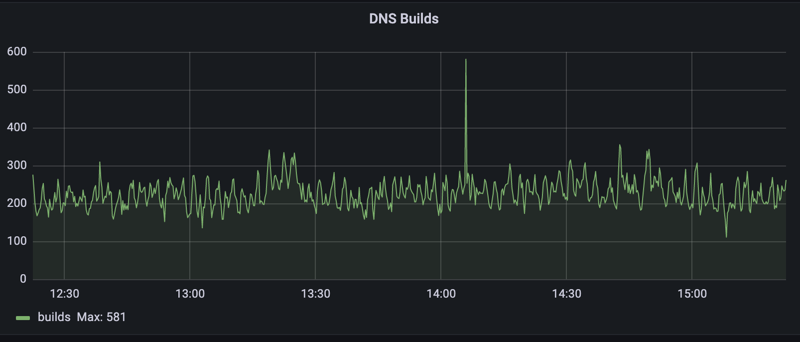
Making our API faster is awesome, but we don’t operate in an isolated environment. Each of these records needs to be processed and pushed to Quicksilver, our distributed database. If we have customers creating tens of thousands of records every 10 seconds, we need to be able to handle this downstream so that we don’t overwhelm our system. In a May 2022 blog post titled How we improved DNS record build speed by more than 4,000x, I notedthat:
We plan to introduce a batching system that will collect record changes into groups to minimize the number of queries we make to our database and Quicksilver.
This task has since been completed, and our propagation pipeline is now able to batch thousands of record changes into a single database query which can then be published to Quicksilver in order to be propagated to our global network.
Next steps
We have a couple more improvements we may want to bring into the API. We also intend to improve the UI to bring more usability improvements to the dashboard to more easily manage zones. We would love to hear your feedback, so please let us know what you think and if you have any suggestions for improvements.
The automobile industry has undergone a remarkable transformation because of the increasing adoption of electric vehicles (EVs). EVs, known for their sustainability and eco-friendliness, are paving the way for a new era in transportation. As environmental concerns and the push for greener technologies have gained momentum, the adoption of EVs has surged, promising to reshape our mobility landscape.
The surge in EVs brings with it a profound need for data acquisition and analysis to optimize their performance, reliability, and efficiency. In the rapidly evolving EV industry, the ability to harness, process, and derive insights from the massive volume of data generated by EVs has become essential for manufacturers, service providers, and researchers alike.
As the EV market is expanding with many new and incumbent players trying to capture the market, the major differentiating factor will be the performance of the vehicles.
Modern EVs are equipped with an array of sensors and systems that continuously monitor various aspects of their operation including parameters such as voltage, temperature, vibration, speed, and so on. From battery management to motor performance, these data-rich machines provide a wealth of information that, when effectively captured and analyzed, can revolutionize vehicle design, enhance safety, and optimize energy consumption. The data can be used to do predictive maintenance, device anomaly detection, real-time customer alerts, remote device management, and monitoring.
However, managing this deluge of data isn’t without its challenges. As the adoption of EVs accelerates, the need for robust data pipelines capable of collecting, storing, and processing data from an exponentially growing number of vehicles becomes more pronounced. Moreover, the granularity of data generated by each vehicle has increased significantly, making it essential to efficiently handle the ever-increasing number of data points. The challenges include not only the technical intricacies of data management but also concerns related to data security, privacy, and compliance with evolving regulations.
In this blog post, we delve into the intricacies of building a reliable data analytics pipeline that can scale to accommodate millions of vehicles, each generating hundreds of metrics every second using Amazon OpenSearch Ingestion. We also provide guidelines and sample configurations to help you implement a solution.
The following architecture diagram provides a scalable and fully managed modern data streaming platform. The architecture uses Amazon OpenSearch Ingestion to stream data into OpenSearch Service and Amazon Simple Storage Service (Amazon S3) to store the data. The data in OpenSearch powers real-time dashboards. The data can also be used to notify customers of any failures occurring on the vehicle (see Configuring alerts in Amazon OpenSearch Service). The data in Amazon S3 is used for business intelligence and long-term storage.
In the following sections, we focus on the following three critical pieces of the architecture in depth:
1. Amazon MSK to OpenSearch ingestion pipeline
2. Amazon OpenSearch Ingestion pipeline to OpenSearch Service
3. Amazon OpenSearch Ingestion to Amazon S3
Solution Walkthrough
Step 1: MSK to Amazon OpenSearch Ingestion pipeline
Because each electric vehicle streams massive volumes of data to Amazon MSK clusters through AWS IoT Core, making sense of this data avalanche is critical. OpenSearch Ingestion provides a fully managed serverless integration to tap into these data streams.
The Amazon MSK source in OpenSearch Ingestion uses Kafka’s Consumer API to read records from one or more MSK topics. The MSK source in OpenSearch Ingestion seamlessly connects to MSK to ingest the streaming data into OpenSearch Ingestion’s processing pipeline.
The following snippet illustrates the pipeline configuration for an OpenSearch Ingestion pipeline used to ingest data from an MSK cluster.
While creating an OpenSearch Ingestion pipeline, add the following snippet in the Pipeline configuration section.
version: "2"
msk-pipeline:
  source:
    kafka:
      acknowledgments: true
      topics:
         - name: "ev-device-topic "
           group_id: "opensearch-consumer"
           serde_format: json
      aws:
        # Provide the Role ARN with access to MSK. This role should have a trust relationship with osis-pipelines.amazonaws.com
        sts_role_arn: "arn:aws:iam:: ::<<account-id>>:role/opensearch-pipeline-Role"
        # Provide the region of the domain.
        region: "<<region>>"
        msk:
          # Provide the MSK ARN.
          arn: "arn:aws:kafka:<<region>>:<<account-id>>:cluster/<<name>>/<<id>>"
When configuring Amazon MSK and OpenSearch Ingestion, it’s essential to establish an optimal relationship between the number of partitions in your Kafka topics and the number of OpenSearch Compute Units (OCUs) allocated to your ingestion pipelines. This optimal configuration ensures efficient data processing and maximizes throughput. You can read more about it in Configure recommended compute units (OCUs) for the Amazon MSK pipeline.
Step 2: OpenSearch Ingestion pipeline to OpenSearch Service
OpenSearch Ingestion offers a direct method for streaming EV data into OpenSearch. The OpenSearch sink plugin channels data from multiple sources directly into the OpenSearch domain. Instead of manually provisioning the pipeline, you define the capacity for your pipeline using OCUs. Each OCU provides 6 GB of memory and two virtual CPUs. To use OpenSearch Ingestion auto-scaling optimally, it’s essential to configure the maximum number of OCUs for a pipeline based on the number of partitions in the topics being ingested. If a topic has a large number of partitions (for example, more than 96, which is the maximum OCUs per pipeline), it’s recommended to configure the pipeline with a maximum of 1–96 OCUs. This way, the pipeline can automatically scale up or down within this range as needed. However, if a topic has a low number of partitions (for example, fewer than 96), it’s advisable to set the maximum number of OCUs to be equal to the number of partitions. This approach ensures that each partition is processed by a dedicated OCU enabling parallel processing and optimal performance. In scenarios where a pipeline ingests data from multiple topics, the topic with the highest number of partitions should be used as a reference to configure the maximum OCUs. Additionally, if higher throughput is required, you can create another pipeline with a new set of OCUs for the same topic and consumer group, enabling near-linear scalability.
OpenSearch Ingestion provides several pre-defined configuration blueprints that can help you quickly build your ingestion pipeline on AWS
The following snippet illustrates pipeline configuration for an OpenSearch Ingestion pipeline using OpenSearch as a SINK with a dead letter queue (DLQ) to Amazon S3. When a pipeline encounters write errors, it creates DLQ objects in the configured S3 bucket. DLQ objects exist within a JSON file as an array of failed events.
sink:
      - opensearch:
          # Provide an AWS OpenSearch Service domain endpoint
          hosts: [ "https://<<domain-name>>.<<region>>.es.amazonaws.com" ]
          aws:
          # Provide a Role ARN with access to the domain. This role should have a trust relationship with osis-pipelines.amazonaws.com
            sts_role_arn: "arn:aws:iam::<<account-id>>:role/<<role-name>>"
          # Provide the region of the domain.
            region: "<<region>>"
          # Enable the 'serverless' flag if the sink is an Amazon OpenSearch Serverless collection
          # serverless: true
          # index name can be auto-generated from topic name
          index: "index_ev_pipe-%{yyyy.MM.dd}"
          # Enable 'distribution_version' setting if the AWS OpenSearch Service domain is of version Elasticsearch 6.x
          #distribution_version: "es6"
          # Enable the S3 DLQ to capture any failed requests in Ohan S3 bucket
          dlq:
            s3:
            # Provide an S3 bucket
              bucket: "<<bucket-name>>"
            # Provide a key path prefix for the failed requests
              key_path_prefix: "oss-pipeline-errors/dlq"
            # Provide the region of the bucket.
              region: "<<region>>"
            # Provide a Role ARN with access to the bucket. This role should have a trust relationship with osis-pipelines.amazonaws.com
              sts_role_arn: "arn:aws:iam:: <<account-id>>:role/<<role-name>>"
Step 3: OpenSearch Ingestion to Amazon S3
OpenSearch Ingestion offers a built-in sink for loading streaming data directly into S3. The service can compress, partition, and optimize the data for cost-effective storage and analytics in Amazon S3. Data loaded into S3 can be partitioned for easier query isolation and lifecycle management. Partitions can be based on vehicle ID, date, geographic region, or other dimensions as needed for your queries.
The following snippet illustrates how we’ve partitioned and stored EV data in Amazon S3.
- s3:
            aws:
              # Provide a Role ARN with access to the bucket. This role should have a trust relationship with osis-pipelines.amazonaws.com
                sts_role_arn: "arn:aws:iam::<<account-id>>:role/<<role-name>>"
              # Provide the region of the domain.
                region: "<<region>>"
            # Replace with the bucket to send the logs to
            bucket: "evbucket"
            object_key:
              # Optional path_prefix for your s3 objects
              path_prefix: "index_ev_pipe/year=%{yyyy}/month=%{MM}/day=%{dd}/hour=%{HH}"
            threshold:
              event_collect_timeout: 60s
            codec:
              parquet:
                auto_schema: true
The following is the complete pipeline configuration, combining the configuration of all three steps. Update the Amazon Resource Names (ARNs), AWS Region, Open Search Service domain endpoint, and S3 names as needed.
The entire OpenSearch Ingestion pipeline configuration can be directly copied into the ‘Pipeline configuration’ field in the AWS Management Console while creating the OpenSearch Ingestion pipeline
version: "2"
msk-pipeline:
  source:
    kafka:
      acknowledgments: true           # Default is false
      topics:
         - name: "<<msk-topic-name>>"
           group_id: "opensearch-consumer"
           serde_format: json
      aws:
        # Provide the Role ARN with access to MSK. This role should have a trust relationship with osis-pipelines.amazonaws.com
        sts_role_arn: "arn:aws:iam::<<account-id>>:role/<<role-name>>"
        # Provide the region of the domain.
        region: "<<region>>"
        msk:
          # Provide the MSK ARN.
          arn: "arn:aws:kafka:us-east-1:<<account-id>>:cluster/<<cluster-name>>/<<cluster-id>>"
  processor:
      - parse_json:
  sink:
      - opensearch:
          # Provide an AWS OpenSearch Service domain endpoint
          hosts: [ "https://<<opensearch-service-domain-endpoint>>.us-east-1.es.amazonaws.com" ]
          aws:
          # Provide a Role ARN with access to the domain. This role should have a trust relationship with osis-pipelines.amazonaws.com
            sts_role_arn: "arn:aws:iam::<<account-id>>:role/<<role-name>>"
          # Provide the region of the domain.
            region: "<<region>>"
          # Enable the 'serverless' flag if the sink is an Amazon OpenSearch Serverless collection
          # index name can be auto-generated from topic name
          index: "index_ev_pipe-%{yyyy.MM.dd}"
          # Enable 'distribution_version' setting if the AWS OpenSearch Service domain is of version Elasticsearch 6.x
          #distribution_version: "es6"
          # Enable the S3 DLQ to capture any failed requests in Ohan S3 bucket
          dlq:
            s3:
            # Provide an S3 bucket
              bucket: "<<bucket-name>>"
            # Provide a key path prefix for the failed requests
              key_path_prefix: "oss-pipeline-errors/dlq"
            # Provide the region of the bucket.
              region: "<<region>>"
            # Provide a Role ARN with access to the bucket. This role should have a trust relationship with osis-pipelines.amazonaws.com
              sts_role_arn: "arn:aws:iam::<<account-id>>:role/<<role-name>>"
      - s3:
            aws:
              # Provide a Role ARN with access to the bucket. This role should have a trust relationship with osis-pipelines.amazonaws.com
                sts_role_arn: "arn:aws:iam::<<account-id>>:role/<<role-name>>"
              # Provide the region of the domain.
                region: "<<region>>"
            # Replace with the bucket to send the logs to
            bucket: "<<bucket-name>>"
            object_key:
              # Optional path_prefix for your s3 objects
              path_prefix: "index_ev_pipe/year=%{yyyy}/month=%{MM}/day=%{dd}/hour=%{HH}"
            threshold:
              event_collect_timeout: 60s
            codec:
              parquet:
                auto_schema: true
Real-time analytics
After the data is available in OpenSearch Service, you can build real-time monitoring and notifications. OpenSearch Service has robust support for multiple notification channels, allowing you to receive alerts through services like Slack, Chime, custom webhooks, Microsoft Teams, email, and Amazon Simple Notification Service (Amazon SNS).
The following screenshot illustrates supported notification channels in OpenSearch Service.
The notification feature in OpenSearch Service allows you to create monitors that will watch for certain conditions or changes in your data and launch alerts, such as monitoring vehicle telemetry data and launching alerts for issues like battery degradation or abnormal energy consumption. For example, you can create a monitor that analyzes battery capacity over time and notifies the on-call team using Slack if capacity drops below expected degradation curves in a significant number of vehicles. This could indicate a potential manufacturing defect requiring investigation.
In addition to notifications, OpenSearch Service makes it easy to build real-time dashboards to visually track metrics across your fleet of vehicles. You can ingest vehicle telemetry data like location, speed, fuel consumption, and so on, and visualize it on maps, charts, and gauges. Dashboards can provide real-time visibility into vehicle health and performance.
The following screenshot illustrates creating a sample dashboard on OpenSearch Service
A key benefit of OpenSearch Service is its ability to handle high sustained ingestion and query rates with millisecond latencies. It distributes incoming vehicle data across data nodes in a cluster for parallel processing. This allows OpenSearch to scale out to handle very large fleets while still delivering the real-time performance needed for operational visibility and alerting.
Batch analytics
After the data is available in Amazon S3, you can build a secure data lake to power a variety of analytics use cases deriving powerful insights. As an immutable store, new data is continually stored in S3 while existing data remains unaltered. This serves as a single source of truth for downstream analytics.
For business intelligence and reporting, you can analyze trends, identify insights, and create rich visualizations powered by the data lake. You can use Amazon QuickSight to build and share dashboards without needing to set up servers or infrastructure. Here’s an example of a Quicksight dashboard for IoT device data. For example, you can use a dashboard to gain insights from historical data that can help with better vehicle and battery design.
You should consider Amazon OpenSearch dashboards for your operational day-to-day use cases to identify issues and alert in near real time whereas Amazon Quicksight should be used to analyze big data stored in a lake house and generate actionable insights from them.
Clean up
Delete the OpenSearch pipeline and Amazon MSK cluster to stop incurring costs on these services.
Conclusion
In this post, you learned how Amazon MSK, OpenSearch Ingestion, OpenSearch Services, and Amazon S3 can be integrated to ingest, process, store, analyze, and act on endless streams of EV data efficiently.
With OpenSearch Ingestion as the integration layer between streams and storage, the entire pipeline scales up and down automatically based on demand. No more complex cluster management or lost data from bursts in streams.
Ayush Agrawal is a Startups Solutions Architect from Gurugram, India with 11 years of experience in Cloud Computing. With a keen interest in AI, ML, and Cloud Security, Ayush is dedicated to helping startups navigate and solve complex architectural challenges. His passion for technology drives him to constantly explore new tools and innovations. When he’s not architecting solutions, you’ll find Ayush diving into the latest tech trends, always eager to push the boundaries of what’s possible.
Fraser Sequeira is a Solutions Architect with AWS based in Mumbai, India. In his role at AWS, Fraser works closely with startups to design and build cloud-native solutions on AWS, with a focus on analytics and streaming workloads. With over 10 years of experience in cloud computing, Fraser has deep expertise in big data, real-time analytics, and building event-driven architecture on AWS.
In the domain of data processing, data analysts run their ad hoc queries on the data lake. The lake serves as an interface between our analytics and production environment, preventing downstream queries from impacting upstream data ingestion pipelines. To ensure efficient data processing in the data lake, choosing appropriate storage formats is crucial.
The vanilla data lake solution is built on top of cloud object storage with Hive metastore, where data files are written in Parquet format. Although this setup is optimised for scalable analytics query patterns, it struggles to handle frequent updates to the data due to two reasons:
The Hive table format requires us to rewrite the Parquet files with the latest data. For instance, to update one record in a Hive unpartitioned table, we would need to read all the data, update the record, and write back the entire data set.
Writing Parquet files is expensive due to the overhead of organising the data to a compressed columnar format, which is more complex than a row format.
The issue is further exacerbated by the scheduled downstream transformations. These necessary steps, which clean and process the data for use, increase the latency because the total delay now includes the combined scheduled intervals of these processing jobs.
Fortunately, the introduction of the Hudi format, which supports fast writes by allowing Avro and Parquet files to co-exist on a Merge On Read (MOR) table, opens up the possibility of having a data lake with minimal data latency. The concept of a commit timeline further allows data to be served with Atomicity, Consistency, Isolation, and Durability (ACID) guarantees.
We employ different sets of configurations for the different characteristics of our input sources:
High or low throughput. A high-throughput source refers to one that has a high level of activity. One example of this can be our stream of booking events generated from each customer transaction. On the other hand, a low-throughput source would be one that has a relative low level of activity. An example of this can be transaction events generated from reconciliation happening on a nightly basis.
Kafka (unbounded) or Relational Database Sources (bounded). Our sinks have sources that can be broadly categorised into unbounded and bounded sources. Unbounded sources are usually related to transaction events materialised as Kafka topics, representing user-generated events as they interact with the Grab superapp. Bounded sources usually refer to Relational Database (RDS) sources, whose size is bound to storage provisioned.
The following sections will delve into the differences between each source and our corresponding configurations optimised for them.
High throughput source
For our data sources with high throughput, we have chosen to write the files in MOR format since the writing of files in Avro format allows for fast writes to meet our latency requirements.
Figure 1 Architecture for MOR tables
As seen in Figure 1, we use Flink to perform the stream processing and write out log files in Avro format in our setup. We then set up a separate Spark writer which periodically converts the Avro files into Parquet format in the Hudi compaction process.
We have further simplified the coordination between the Flink and Spark writers by enabling asynchronous services on the Flink writer so it can generate the compaction plans for Spark writers to act on. During the Spark job runs, it checks for available compaction plans and acts on them, placing the burden of orchestrating the writes solely on the Flink writer. This approach could help minimise potential concurrency problems that might otherwise arise, as there would be a single actor
orchestrating the associated Hudi table services.
Low throughput source
Figure 2 Architecture for COW tables
For low throughput sources, we gravitate towards the choice of Copy On Write (COW) tables given the simplicity of its design, since it only involves one component, which is the Flink writer. The downside is that it has higher data latency because this setup only generates Parquet format data snapshots at each checkpoint interval, which is typically about 10-15 minutes.
Connecting to our Kafka (unbounded) data source
Grab uses Protobuf as our central data format in Kafka, ensuring schema evolution compatibility. However, the derivation of the schema of these topics still requires some transformation to make it compatible with Hudi’s accepted schema. Some of these transformations include ensuring that Avro record fields do not contain just a single array field, and handling logical decimal schemas to transform them to fixed byte schema for Spark compatibility.
Given the unbounded nature of the source, we decided to partition it by Kafka event time up to the hour level. This ensured that our Hudi operations would be faster. Parquet file writes would be faster since they would only affect files within the same partition, and each Parquet file within the same event time partition would have a bounded size given the monotonically increasing nature of Kafka event time.
By partitioning tables by Kafka event time, we can further optimise compaction planning operations, since the amount of file lookups required is now reduced with the use of BoundedPartitionAwareCompactionStrategy. Only log files in recent partitions would be selected for compaction and the job manager need not list every partition to figure out which log files to select for compaction during the planning phase anymore.
Connecting to our RDS (bounded) data source
For our RDS, we decided to use the Flink Change Data Capture (CDC) connectors by Veverica to obtain the binlog streams. The RDS would then treat the Flink writer as a replication server and start streaming its binlog data to it for each MySQL change. The Flink CDC connector presents the data as a Kafka Connect (KC) Source record, since it uses the Debezium connector under the hood. It is then a straightforward task to deserialise these records and transform them into Hudi records, since
the Avro schema and associated data changes are already captured within the KC source record.
The obtained binlog timestamp is also emitted as a metric during consumption for us to monitor the observed data latency at the point of ingestion.
Optimising for these sources involves two phases:
First, assigning more resources for the cold start incremental snapshot process where Flink takes a snapshot of the current data state in the RDS and loads the Hudi table with that snapshot. This phase is usually resource-heavy as there are a lot of file writes and data ingested during this process.
Once the snapshotting is completed, Flink would then start to process the binlog stream and the observed throughput would drop to a level similar to the DB write throughput. The resources required by the Flink writer at this stage would be much lower than in the snapshot phase.
Indexing for Hudi tables
Indexing is important for upserting Hudi tables when the writing engine performs updates, allowing it to efficiently locate the file groups of the data to be updated.
As of version 0.14, the Flink engine only supports Bucket Index or Flink State Index. Bucket Index performs indexing of the file record by hashing the record key and matching it to a specific bucket of files indicated by the naming convention of the written data files. Flink State Index on the other hand stores the index map of record keys to files in memory.
Given that our tables include unbounded Kafka sources, there is a possibility for our state indexes to grow indefinitely. Furthermore, the requirement of state preservation for Flink State Index across version deployments and configuration updates adds complexity to the overall solution.
Thus, we opted for the simple Bucket Index for its simplicity and the fact that our Hudi table size per partition does not change drastically across the week. However, this comes with a limitation whereby the number of buckets cannot be updated easily and imposes a parallelism limit at which our Flink pipelines can scale. Thus, as traffic grows organically, we would find ourselves in a situation whereby our configuration grows obsolete and cannot handle the increased load.
To resolve this going forward, using consistent hashing for the Bucket Index would be something to explore to optimise our Parquet file sizes and allow the number of buckets to grow seamlessly as traffic grows.
Impact
Fresh business metrics
Post creation of our Hudi Data Ingestion solution, we have enabled various users such as our data analysts to perform ad hoc queries much more easily on data that has lower latency. Furthermore, Hudi tables can be seamlessly joined with Hive tables in Trino for additional context. This enabled the construction of operational dashboards reflecting fresh business metrics to our various operators, empowering them with the necessary information to quickly respond to any abnormalities (such as high-demand events like F1 or seasonal holidays).
Quicker fraud detection
Another significant user of our solution is our fraud detection analysts. This enabled them to rapidly access fresh transaction events and analyse them for fraudulent patterns, particularly during the emergence of a new attack pattern that hadn’t been detected by their rules engine. Our solution also allowed them to perform multiple ad hoc queries that involve lookbacks of various days’ worth of data without impacting our production RDS and Kafka clusters by using the data lake as the data interface, reducing the data latency to the minute level and, in turn, empowering them to respond more quickly to attacks.
What’s next?
As the landscape of data storage solutions evolves rapidly, we are eager to test and integrate new features like Record Level Indexing and the creation of Pre Join tables. This evolution extends beyond the Hudi community to other table formats such as IceBerg and DeltaLake. We remain ready to adapt ourselves to these changes and incorporate the advantages of each format into our data lake within Grab.
Grab is the leading superapp platform in Southeast Asia, providing everyday services that matter to consumers. More than just a ride-hailing and food delivery app, Grab offers a wide range of on-demand services in the region, including mobility, food, package and grocery delivery services, mobile payments, and financial services across 428 cities in eight countries.
Powered by technology and driven by heart, our mission is to drive Southeast Asia forward by creating economic empowerment for everyone. If this mission speaks to you, join our team today!
In this digital age, companies collect multitudes of data that enable the tracking of business metrics and performance. Over the years, data analytics tools for data storage and processing have evolved from the days of Excel sheets and macros to more advanced Map Reduce model tools like Spark, Hadoop, and Hive. This evolution has allowed companies, including Grab, to perform modern analytics on the data ingested into the Data Lake, empowering them to make better data-driven business decisions. This form of data will be referenced within this document as “Offline Data”.
With innovations in stream processing technology like Spark and Flink, there is now more interest in unlocking value from streaming data. This form of continuously-generated data in high volume will be referenced within this document as “Online Data”. In the context of Grab, the streaming data is usually materialised as Kafka topics (“Kafka Stream”) as the result of stream processing in its framework. This data is largely unexplored until they are eventually sunk into the Data Lake as Offline Data, part of the data journey (see Figure 1 below). This induces some data latency before the data can be used by data analysts to inform decisions.
Figure 1. Simplified data journey for Offline Data vs. Online Data, from data generation to data analysis.
As seen in Figure 1 above, the Time to Value (“TTV”) of Online Data is shorter as compared to that of Offline Data in a simplified data journey from data generation to data analysis where complexities of data cleaning and transformation have been removed. This is because the role of the data analyst or data scientist (“Data End User”) has been enabled forward to the Kafka stage for Online Data instead of the Data Lake stage for Offline Data. We recognise that allowing earlier data exploration on Online Data allows Data End Users to build context around the data inputs they are using in an earlier stage. This can help them process Offline Data more meaningfully in subsequent stages. We are interested in opening up the possibility for Data End Users to at least explore the Online Data before they architect a full solution to clean and/or process the data directly or more efficiently post-ingestion into the Data Lake. After their data exploration, the users would have more information to decide whether to spin up a stream processing pipeline for Online Data, or to continue processing Offline Data with their current solution, but with a more refined understanding and logic strategy against their source data inputs. However, of course, in this blog, we acknowledge that not all analysis on Online Data could be done in this manner.
Problem statement
Online Data is underutilised within Grab mainly because of, among other reasons, difficulty in performing data exploration on data that is not yet properly stored in the Data Lake.
For the purpose of this blog post, we will focus only on the problem of exploration of Online Data because this problem is the precursor to allowing us to fully democratise such data.
The problem of data exploration manifests itself when Data End Users need to find the proper data inputs to base and develop their data models. These users would then often need to parse through a multitude of documentation and connect with multiple upstream data producers, to know the range of data signals that are currently available and understand what each data signal is trying to measure.
Given the ephemeral nature of Online Data, this implies that the lack of correct tool adoption to seamlessly perform quick tests with application logic on Online Data disincentivises the Data End Users to work on these Online Data. Testing such logic on Offline Data is generally much easier since iteration testing on the exact same dataset is possible.
This difficulty in performing data exploration including ad hoc queries on Online Data has therefore made development of stream processing applications hard for Data End Users, creating headwinds in Grab’s aim to evolve from making data-driven business decisions to also making data-driven operation decisions. Doing both would allow Grab to react much quicker to abrupt changes in its business landscape.
Adoption of Zeppelin notebook environment
To address the difficulty in performing data exploration on Online Data, we have adopted Apache Zeppelin, a web-based notebook that enables data-drive, interactive data analytics with the support of multiple interpreters to work with various data processing backends e.g. Spark, Flink. The full solution of the adopted Zeppelin notebook environment is enabled seamlessly within our internal data-streaming platform, through its control plane. If you are interested, you may check out our previous blog post titled An elegant platform for more details on the abovementioned streaming platform and its control plane.
Figure 2. Zeppelin login page via web-based notebook environment.
As seen from Figure 2 above, after successful creation of the Zeppelin cluster, users can log in with their generated credentials delivered to them via the integrated instant messenger, and start using the notebook environment.
Figure 3. Zeppelin programme flow in the notebook environment.
Figure 3 above explains the Zeppelin notebook programme flow as follows:
The users enter their queries into the notebook session and run querying statements interactively with the established web-based notebook session.
The queries are passed to the Flink interpreter within the cluster to generate the Flink job as a Jar file, to be then submitted to a Flink session cluster.
When the Flink session cluster job manager receives the job, it would spin up the corresponding Flink task managers (workers) to run the application and retrieve the results.
The query results would then be piped back to the notebook session, to be displayed back to the user on the notebook session.
Data query and visualisation
Figure 4. Example of simple select query of data on Kafka. Note: All variable names, schema, values, and other details used in this article are only created for use as examples.
Flink has a planned roadmap to create a unified streaming language for both stream processing and data analytics. In line with the roadmap, we have based our Zeppelin solution on supporting Structured Query Language (“SQL”) as the query language of choice as seen in Figure 4 above. Data End Users can now write queries in SQL, which is a language that they are comfortable with, and perform adequate data exploration.
As discussed in this section, data exploration on streaming data at the Kafka stage by adopting the right tool enables Data End Users to seamlessly have visibility to quickly understand the current schema of a Kafka topic (explained more in the next section. This kind of data exploration also enables Data End Users to understand the type of data the Kafka topic represents, such as the ability to determine if a country code data field is in alpha-2 or alpha-3 format while the data is still part of streaming data. This might seem inconsequential and immediately identifiable even in Offline Data, but by enabling data exploration at an earlier stage in the data journey for Online Data, Data End Users have the opportunity to react much more quickly. For example, a change of expected country code format from the data producer would usually lead to errors in the downstream joins or other stream processing pipelines due to incompatible parsing or filtering of the modified country codes. Instead of waiting for the data to be ingested to Offline Data, users can investigate the issue with Online Data retrieved from Kafka.
Figure 5. Simple visualisation of queried data on Zeppelin’s notebook environment. Note: All variable names, schema, values, and other details used in this article are only created for use as examples.
Besides query features, Zeppelin notebook provides simple visualisation and analytics of the off-the-shelf data as presented above in Figure 5. Furthermore, users are now able to perform interactive ad hoc queries on Online Data. These queries will eventually become much more advanced and/or effective SQL queries to be deployed as a streaming pipeline later on in the data journey. This reduces the inertia in setting up a separate development environment or learning other programming languages like Java or Scala during the development of streaming pipelines. With Zeppelin’s notebook environment, our Data End Users are more empowered to quickly derive value from Online Data.
Need for a more dynamic table schema derivation process
For the Data End Users performing data exploration on Online Data, we see a need for these users to derive the Data Definition Language (“DDL”) associated with a Kafka stream at an earlier stage of the data journey. Within Grab, even though Kafka streams are transmitted in Protobuf format and are thus structured, both the schema and the corresponding DDL changes are added over time as new fields. Typically, the data producer (service owners) and the data engineers responsible for the data ingestion pipeline coordinate to perform such updates. Since the Data End Users are not involved in such schema update processes nor do they directly interact with the data producers, many of them find the discovery of changes in the current Kafka stream schema an issue. Granted that this is an issue our metadata platform is actively solving using Datahub, we hope to also solve the challenge by being able to derive the DDL more dynamically within the tooling, for data exploration on Online Data to reduce friction.
Figure 6. Common functions to derive DDL of a Kafka Stream in SQL. Note: All variable names, schema, values, and other details used in this article are only created for use as examples.
As seen from Figure 6 above, we have an integrated tooling for Data End Users to derive the DDL associated with a Kafka stream using SQL language. A Kafka stream in Grab’s context is a logical concept describing a Kafka topic, associating it with its metadata like Kafka bootstrap servers and associated Java class created by Protoc. This tool maps the Protobuf schema definition of a Kafka stream to a DDL, allowing it to be expressed and used in SQL language. This reduces the manual effort involved in creating these table definitions from scratch based on the associated Protobuf schema. Users can now derive the DDL associated with a Kafka stream more easily.
Mitigating risks arising from data exploration on Online Data – data access authorisation/audit
While we rethink stream processing and are open to options that enable data exploration on Online Data as mentioned above, we realised that new security requirements related to data access authorisation and maintaining proper audit trail have emerged. Even with Personally Identifiable Information (PII) obfuscation enforcement by our streaming pipeline, it means we need to implement stricter guardrails in place along with audit trails to ensure users only have access to what they are allowed to, and this access can be removed in a break-glass scenario. If you are interested, you may check out our previous blog post titled PII masking for privacy-grade machine learning for more details about how we enforce PII masking on machine learning data streaming pipelines.
To enable data access authorisation, we utilised Strimzi, the operator of running Kafka on Kubernetes. We integrated Strimzi’s Open Policy Agent (OPA) with Kafka to define policies that authorise specific read-only user access to specific Kafka Topics. The identification of users is done via mutualTLS (mTLS) connection with our Kafka clusters, where their user details are part of the SSL certificate details used for authentication.
With these tools in place, each user’s request to explore Online Data would be properly logged, and each data access can be controlled by an OPA policy managed by a central team.
If you are interested, you may check out our previous post Zero trust with Kafka where we discussed our efforts to continue strengthening the security of our data-streaming platform.
Impact
With the proliferation of our data-streaming platform, we expect to see improvements in the way our data becomes gradually democratised. We have already been receiving use cases from the Data End Users who are interested in validating a chain of events on Online Data, i.e. retrieving information of all events associated with a particular booking, which is not currently something that can be done easily.
More importantly, the tools in place for data exploration on Online Data form the foundation required for us to embark on our next step of the stream processing journey. This foundation makes the development and validation of the stream processing logic much quicker. This occurs when ad hoc queries in a notebook environment are possible, removing the need for local developer environment setups and the need to go through the whole pipeline deployment process for eventual validation of the developed logic. We believe that this would prove to reduce our lead time in creating stream processing pipelines significantly.
What’s next?
Our next step is to rethink further how our stream processing pipelines are defined and start to provision SQL as the unified streaming language of our pipelines. This helps facilitate better discussion between upstream data producers, data engineers, and Data End Users, since SQL is the common language among these stakeholders.
We will also explore handling schema discovery in a more controlled manner by utilising a Hive catalogue to store our Kafka table definitions. This removes the need for users to retrieve and run the table DDL statement for every session, making the data exploration experience even more seamless.
Grab is the leading superapp platform in Southeast Asia, providing everyday services that matter to consumers. More than just a ride-hailing and food delivery app, Grab offers a wide range of on-demand services in the region, including mobility, food, package and grocery delivery services, mobile payments, and financial services across 428 cities in eight countries.
Powered by technology and driven by heart, our mission is to drive Southeast Asia forward by creating economic empowerment for everyone. If this mission speaks to you, join our team today!
Coban – Grab’s real-time data streaming platform – has been operating Kafka on Kubernetes with Strimzi in
production for about two years. In a previous article (Zero trust with Kafka), we explained how we leveraged Strimzi to enhance the security of our data streaming offering.
In this article, we are going to describe how we improved the fault tolerance of our initial design, to the point where we no longer need to intervene if a Kafka broker is unexpectedly terminated.
To make our operations easier and limit the blast radius of any incidents, we deploy exactly one Kafka cluster for each EKS cluster. We also give a full worker node to each Kafka broker. In terms of storage, we initially relied on EC2 instances with non-volatile memory express (NVMe) instance store volumes for
maximal I/O performance. Also, each Kafka cluster is accessible beyond its own Virtual Private Cloud (VPC) via a VPC Endpoint Service.
Fig. 1 Initial design of a 3-node Kafka cluster running on Kubernetes.
Fig. 1 shows a logical view of our initial design of a 3-node Kafka on Kubernetes cluster, as typically run by Coban. The Zookeeper and Cruise-Control components are not shown for clarity.
There are four Kubernetes services (1): one for the initial connection – referred to as “bootstrap” – that redirects incoming traffic to any Kafka pods, plus one for each Kafka pod, for the clients to target each Kafka broker individually (a requirement to produce or consume from/to a partition that resides on any particular Kafka broker). Four different listeners on the Network Load Balancer (NLB) listening on four different TCP ports, enable the Kafka clients to target either the bootstrap
service or any particular Kafka broker they need to reach. This is very similar to what we previously described in Exposing a Kafka Cluster via a VPC Endpoint Service.
Each worker node hosts a single Kafka pod (2). The NVMe instance store volume is used to create a Kubernetes Persistent Volume (PV), attached to a pod via a Kubernetes Persistent Volume Claim (PVC).
Lastly, the worker nodes belong to Auto-Scaling Groups (ASG) (3), one by Availability Zone (AZ). Strimzi adds in node affinity to make sure that the brokers are evenly distributed across AZs. In this initial design, ASGs are not for auto-scaling though, because we want to keep the size of the cluster under control. We only use ASGs – with a fixed size – to facilitate manual scaling operation and to automatically replace the terminated worker nodes.
With this initial design, let us see what happens in case of such a worker node termination.
Fig. 2 Representation of a worker node termination. Node C is terminated and replaced by node D. However the Kafka broker 3 pod is unable to restart on node D.
Fig. 2 shows the worker node C being terminated along with its NVMe instance store volume C, and replaced (by the ASG) by a new worker node D and its new, empty NVMe instance store volume D. On start-up, the worker node D automatically joins the Kubernetes cluster. The Kafka broker 3 pod that was running on the faulty worker node C is scheduled to restart on the new worker node D.
Although the NVMe instance store volume C is terminated along with the worker node C, there is no data loss because all of our Kafka topics are configured with a minimum of three replicas. The data is poised to be copied over from the surviving Kafka brokers 1 and 2 back to Kafka broker 3, as soon as Kafka broker 3 is effectively restarted on the worker node D.
However, there are three fundamental issues with this initial design:
The Kafka clients that were in the middle of producing or consuming to/from the partition leaders of Kafka broker 3 are suddenly facing connection errors, because the broker was not gracefully demoted beforehand.
The target groups of the NLB for both the bootstrap connection and Kafka broker 3 still point to the worker node C. Therefore, the network communication from the NLB to Kafka broker 3 is broken. A manual reconfiguration of the target groups is required.
The PVC associating the Kafka broker 3 pod with its instance store PV is unable to automatically switch to the new NVMe instance store volume of the worker node D. Indeed, static provisioning is an intrinsic characteristic of Kubernetes local volumes. The PVC is still in Bound state, so Kubernetes does not take any action. However, the actual storage beneath the PV does not exist anymore. Without any storage, the Kafka broker 3 pod is unable to start.
At this stage, the Kafka cluster is running in a degraded state with only two out of three brokers, until a Coban engineer intervenes to reconfigure the target groups of the NLB and delete the zombie PVC (this, in turn, triggers its re-creation by Strimzi, this time using the new instance store PV).
In the next section, we will see how we have managed to address the three issues mentioned above to make this design fault-tolerant.
Solution
Graceful Kafka shutdown
To minimise the disruption for the Kafka clients, we leveraged the AWS Node Termination Handler (NTH). This component provided by AWS for Kubernetes environments is able to cordon and drain a worker node that is going to be terminated. This draining, in turn, triggers a graceful shutdown of the Kafka
process by sending a polite SIGTERM signal to all pods running on the worker node that is being drained (instead of the brutal SIGKILL of a normal termination).
The termination events of interest that are captured by the NTH are:
Scale-in operations by an ASG.
Manual termination of an instance.
AWS maintenance events, typically EC2 instances scheduled for upcoming retirement.
This suffices for most of the disruptions our clusters can face in normal times and our common maintenance operations, such as terminating a worker node to refresh it. Only sudden hardware failures (AWS issue events) would fall through the cracks and still trigger errors on the Kafka client side.
Fig. 3 Architecture of the NTH with the Queue Processor.
Fig. 3 shows the NTH with the Queue Processor in action, and how it reacts to a scale-in operation (typically triggered manually, during a maintenance operation):
As soon as the scale-in operation is triggered, an Auto Scaling lifecycle hook is invoked to pause the termination of the instance.
Simultaneously, an Auto Scaling lifecycle hook event is issued to an Amazon Simple Queue Service (SQS) queue. In Fig. 3, we have also materialised EC2 events (e.g. manual termination of an instance, AWS maintenance events, etc.) that transit via Amazon EventBridge to eventually end up in the same SQS queue. We will discuss EC2 events in the next two sections.
The NTH, a pod running in the Kubernetes cluster itself, constantly polls that SQS queue.
When a scale-in event pertaining to a worker node of the Kubernetes cluster is read from the SQS queue, the NTH sends to the Kubernetes API the instruction to cordon and drain the impacted worker node.
On draining, Kubernetes sends a SIGTERM signal to the Kafka pod residing on the worker node.
Upon receiving the SIGTERM signal, the Kafka pod gracefully migrates the leadership of its leader partitions to other brokers of the cluster before shutting down, in a transparent manner for the clients. This behaviour is ensured by the controlled.shutdown.enable parameter of Kafka, which is enabled by default.
Once the impacted worker node has been drained, the NTH eventually resumes the termination of the instance.
Strimzi also comes with a terminationGracePeriodSeconds parameter, which we have set to 180 seconds to give the Kafka pods enough time to migrate all of their partition leaders gracefully on termination. We have verified that this is enough to migrate all partition leaders on our Kafka clusters (about 60 seconds for 600 partition leaders).
Manual termination of an instance
The Auto Scaling lifecycle hook that pauses the termination of an instance (Fig. 3, step 1) as well as the corresponding resuming by the NTH (Fig. 3, step 7) are invoked only for ASG scaling events.
In case of a manual termination of an EC2 instance, the termination is captured as an EC2 event that also reaches the NTH. Upon receiving that event, the NTH cordons and drains the impacted worker node. However, the instance is immediately terminated, most likely before the leadership of all of its Kafka partition leaders has had the time to get migrated to other brokers.
To work around this and let a manual termination of an EC2 instance also benefit from the ASG lifecycle hook, the instance must be terminated using the terminate-instance-in-auto-scaling-group AWS CLI command.
AWS maintenance events
For AWS maintenance events such as instances scheduled for upcoming retirement, the NTH acts immediately when the event is first received (typically adequately in advance). It cordons and drains the soon-to-be-retired worker node, which in turn triggers the SIGTERM signal and the graceful termination of Kafka as described above. At this stage, the impacted instance is not terminated, so the Kafka partition leaders have plenty of time to complete their migration to other brokers.
However, the evicted Kafka pod has nowhere to go. There is a need for spinning up a new worker node for it to be able to eventually restart somewhere.
To make this happen seamlessly, we doubled the maximum size of each of our ASGs and installed the Kubernetes Cluster Autoscaler. With that, when such a maintenance event is received:
The worker node scheduled for retirement is cordoned and drained by the NTH. The state of the impacted Kafka pod becomes Pending.
The Kubernetes Cluster Autoscaler comes into play and triggers the corresponding ASG to spin up a new EC2 instance that joins the Kubernetes cluster as a new worker node.
The impacted Kafka pod restarts on the new worker node.
The Kubernetes Cluster Autoscaler detects that the previous worker node is now under-utilised and terminates it.
In this scenario, the impacted Kafka pod only remains in Pending state for about four minutes in total.
In case of multiple simultaneous AWS maintenance events, the Kubernetes scheduler would honour our PodDisruptionBudget and not evict more than one Kafka pod at a time.
Dynamic NLB configuration
To automatically map the NLB’s target groups with a newly spun up EC2 instance, we leveraged the AWS Load Balancer Controller (LBC).
Let us see how it works.
Fig. 4 Architecture of the LBC managing the NLB’s target groups via TargetGroupBinding custom resources.
Fig. 4 shows how the LBC automates the reconfiguration of the NLB’s target groups:
It first retrieves the desired state described in Kubernetes custom resources (CR) of type TargetGroupBinding. There is one such resource per target group to maintain. Each TargetGroupBinding CR associates its respective target group with a Kubernetes service.
The LBC then watches over the changes of the Kubernetes services that are referenced in the TargetGroupBinding CRs’ definition, specifically the private IP addresses exposed by their respective Endpoints resources.
When a change is detected, it dynamically updates the corresponding NLB’s target groups with those IP addresses as well as the TCP port of the target containers (containerPort).
This automated design sets up the NLB’s target groups with IP addresses (targetType: ip) instead of EC2 instance IDs (targetType: instance). Although the LBC can handle both target types, the IP address approach is actually more straightforward in our case, since each pod has a routable private IP address in the AWS subnet, thanks to the AWS Container Networking Interface (CNI) plug-in.
This dynamic NLB configuration design comes with a challenge. Whenever we need to update the Strimzi CR, the rollout of the change to each Kafka pod in a rolling update fashion is happening too fast for the NLB. This is because the NLB inherently takes some time to mark each target as healthy before enabling it. The Kafka brokers that have just been rolled out start advertising their broker-specific endpoints to the Kafka clients via the bootstrap service, but those
endpoints are actually not immediately available because the NLB is still checking their health. To mitigate this, we have reduced the HealthCheckIntervalSeconds and HealthyThresholdCount parameters of each target group to their minimum values of 5 and 2 respectively. This reduces the maximum delay for the NLB to detect that a target has become healthy to 10 seconds. In addition, we have configured the LBC with a Pod Readiness Gate. This feature makes the Strimzi rolling deployment wait for the health check of the NLB to pass, before marking the current pod as Ready and proceeding with the next pod.
Fig. 5 Steps for a Strimzi rolling deployment with a Pod Readiness Gate. Only one Kafka broker and one NLB listener and target group are shown for simplicity.
Fig. 5 shows how the Pod Readiness Gate works during a Strimzi rolling deployment:
The old Kafka pod is terminated.
The new Kafka pod starts up and joins the Kafka cluster. Its individual endpoint for direct access via the NLB is immediately advertised by the Kafka cluster. However, at this stage, it is not reachable, as the target group of the NLB still points to the IP address of the old Kafka pod.
The LBC updates the target group of the NLB with the IP address of the new Kafka pod, but the NLB health check has not yet passed, so the traffic is not forwarded to the new Kafka pod just yet.
The LBC then waits for the NLB health check to pass, which takes 10 seconds. Once the NLB health check has passed, the NLB resumes forwarding the traffic to the Kafka pod.
Finally, the LBC updates the pod readiness gate of the new Kafka pod. This informs Strimzi that it can proceed with the next pod of the rolling deployment.
Data persistence with EBS
To address the challenge of the residual PV and PVC of the old worker node preventing Kubernetes from mounting the local storage of the new worker node after a node rotation, we adopted Elastic Block Store (EBS) volumes instead of NVMe instance store volumes. Contrary to the latter, EBS volumes can conveniently be attached and detached. The trade-off is that their performance is significantly lower.
However, relying on EBS comes with additional benefits:
The cost per GB is lower, compared to NVMe instance store volumes.
Using EBS decouples the size of an instance in terms of CPU and memory from its storage capacity, leading to further cost savings by independently right-sizing the instance type and its storage. Such a separation of concerns also opens the door to new use cases requiring disproportionate amounts of storage.
After a worker node rotation, the time needed for the new node to get back in sync is faster, as it only needs to catch up the data that was produced during the downtime. This leads to shorter maintenance operations and higher iteration speed. Incidentally, the associated inter-AZ traffic cost is also lower, since there is less data to transfer among brokers during this time.
Increasing the storage capacity is an online operation.
Data backup is supported by taking snapshots of EBS volumes.
We have verified with our historical monitoring data that the performance of EBS General Purpose 3 (gp3) volumes is significantly above our maximum historical values for both throughput and I/O per second (IOPS), and we have successfully benchmarked a test EBS-based Kafka cluster. We have also set up new monitors to be alerted in case we need to
provision either additional throughput or IOPS, beyond the baseline of EBS gp3 volumes.
With that, we updated our instance types from storage optimised instances to either general purpose or memory optimised instances. We added the Amazon EBS Container Storage Interface (CSI) driver to the Kubernetes cluster and created a new Kubernetes storage class to let the cluster dynamically provision EBS gp3 volumes.
We configured Strimzi to use that storage class to create any new PVCs. This makes Strimzi able to automatically create the EBS volumes it needs, typically when the cluster is first set up, but also to attach/detach the volumes to/from the EC2 instances whenever a Kafka pod is relocated to a different worker node.
Note that the EBS volumes are not part of any ASG Launch Template, nor do they scale automatically with the ASGs.
Fig. 6 Steps for the Strimzi Operator to create an EBS volume and attach it to a new Kafka pod.
Fig. 6 illustrates how this works when Strimzi sets up a new Kafka broker, for example the first broker of the cluster in the initial setup:
The Strimzi Cluster Operator first creates a new PVC, specifying a volume size and EBS gp3 as its storage class. The storage class is configured with the EBS CSI Driver as the volume provisioner, so that volumes are dynamically provisioned [1]. However, because it is also set up with volumeBindingMode: WaitForFirstConsumer, the volume is not yet provisioned until a pod actually claims the PVC.
The Strimzi Cluster Operator then creates the Kafka pod, with a reference to the newly created PVC. The pod is scheduled to start, which in turn claims the PVC.
This triggers the EBS CSI Controller. As the volume provisioner, it dynamically creates a new EBS volume in the AWS VPC, in the AZ of the worker node where the pod has been scheduled to start.
It then attaches the newly created EBS volume to the corresponding EC2 instance.
After that, it creates a Kubernetes PV with nodeAffinity and claimRef specifications, making sure that the PV is reserved for the Kafka broker 1 pod.
Lastly, it updates the PVC with the reference of the newly created PV. The PVC is now in Bound state and the Kafka pod can start.
One important point to take note of is that EBS volumes can only be attached to EC2 instances residing in their own AZ. Therefore, when rotating a worker node, the EBS volume can only be re-attached to the new instance if both old and new instances reside in the same AZ. A simple way to guarantee this is to set up one ASG per AZ, instead of a single ASG spanning across 3 AZs.
Also, when such a rotation occurs, the new broker only needs to synchronise the recent data produced during the brief downtime, which is typically an order of magnitude faster than replicating the entire volume (depending on the overall retention period of the hosted Kafka topics).
Table 1 Comparison of the resynchronization of the Kafka data after a broker rotation between the initial design and the new design with EBS volumes.
Initial design (NVMe instance store volumes)
New design (EBS volumes)
Data to synchronise
All of the data
Recent data produced during the brief downtime
Function of (primarily)
Retention period
Downtime
Typical duration
Hours
Minutes
Outcome
With all that, let us revisit the initial scenario, where a malfunctioning worker node is being replaced by a fresh new node.
Fig. 7 Representation of a worker node termination after implementing the solution. Node C is terminated and replaced by node D. This time, the Kafka broker 3 pod is able to start and serve traffic.
Fig. 7 shows the worker node C being terminated and replaced (by the ASG) by a new worker node D, similar to what we have described in the initial problem statement. The worker node D automatically joins the Kubernetes cluster on start-up.
However, this time, a seamless failover takes place:
The Kafka clients that were in the middle of producing or consuming to/from the partition leaders of Kafka broker 3 are gracefully redirected to Kafka brokers 1 and 2, where Kafka has migrated the leadership of its leader partitions.
The target groups of the NLB for both the bootstrap connection and Kafka broker 3 are automatically updated by the LBC. The connectivity between the NLB and Kafka broker 3 is immediately restored.
Triggered by the creation of the Kafka broker 3 pod, the Amazon EBS CSI driver running on the worker node D re-attaches the EBS volume 3 that was previously attached to the worker node C, to the worker node D instead. This enables Kubernetes to automatically re-bind the corresponding PV and PVC to Kafka broker 3 pod. With its storage dependency resolved, Kafka broker 3 is able to start successfully and re-join the Kafka cluster. From there, it only needs to catch up with the new data that was produced
during its short downtime, by replicating it from Kafka brokers 1 and 2.
With this fault-tolerant design, when an EC2 instance is being retired by AWS, no particular action is required from our end.
Similarly, our EKS version upgrades, as well as any operations that require rotating all worker nodes of the cluster in general, are:
Simpler and less error-prone: We only need to rotate each instance in sequence, with no need for manually reconfiguring the target groups of the NLB and deleting the zombie PVCs anymore.
Faster: The time between each instance rotation is limited to the short amount of time it takes for the restarted Kafka broker to catch up with the new data.
More cost-efficient: There is less data to transfer across AZs (which is charged by AWS).
It is worth noting that we have chosen to omit Zookeeper and Cruise Control in this article, for the sake of clarity and simplicity. In reality, all pods in the Kubernetes cluster – including Zookeeper and Cruise Control – now benefit from the same graceful stop, triggered by the AWS termination events and the NTH. Similarly, the EBS CSI driver improves the fault tolerance of any pods that use EBS volumes for persistent storage, which includes the Zookeeper pods.
Challenges faced
One challenge that we are facing with this design lies in the EBS volumes’ management.
On the one hand, the size of EBS volumes cannot be increased consecutively before the end of a cooldown period (minimum of 6 hours and can exceed 24 hours in some cases [2]). Therefore, when we need to urgently extend some EBS volumes because the size of a Kafka topic is suddenly growing, we need to be relatively generous when sizing the new required capacity and add a comfortable security margin, to make sure that we are not running out of storage in the short run.
On the other hand, shrinking a Kubernetes PV is not a supported operation. This can affect the cost efficiency of our design if we overprovision the storage capacity by too much, or in case the workload of a particular cluster organically diminishes.
One way to mitigate this challenge is to tactically scale the cluster horizontally (ie. adding new brokers) when there is a need for more storage and the existing EBS volumes are stuck in a cooldown period, or when the new storage need is only temporary.
What’s next?
In the future, we can improve the NTH’s capability by utilising webhooks. Upon receiving events from SQS, the NTH can also forward the events to the specified webhook URLs.
This can potentially benefit us in a few ways, e.g.:
Proactively spinning up a new instance without waiting for the old one to be terminated, whenever a termination event is received. This would shorten the rotation time even further.
Sending Slack notifications to Coban engineers to keep them informed of any actions taken by the NTH.
We would need to develop and maintain an application that receives webhook events from the NTH and performs the necessary actions.
In addition, we are also rolling out Karpenter to replace the Kubernetes Cluster Autoscaler, as it is able to spin up new instances slightly faster, helping reduce the four minutes delay a Kafka pod remains in Pending state during a node rotation. Incidentally, Karpenter also removes the need for setting up one ASG by AZ, as it is able to deterministically provision instances in a specific AZ, for example where a particular EBS volume resides.
Lastly, to ensure that the performance of our EBS gp3 volumes is both sufficient and cost-efficient, we want to explore autoscaling their throughput and IOPS beyond the baseline, based on the usage metrics collected by our monitoring stack.
We would like to thank our team members and Grab Kubernetes gurus that helped review and improve this blog before publication: Will Ho, Gable Heng, Dewin Goh, Vinnson Lee, Siddharth Pandey, Shi Kai Ng, Quang Minh Tran, Yong Liang Oh, Leon Tay, Tuan Anh Vu.
Join us
Grab is the leading superapp platform in Southeast Asia, providing everyday services that matter to consumers. More than just a ride-hailing and food delivery app, Grab offers a wide range of on-demand services in the region, including mobility, food, package and grocery delivery services, mobile payments, and financial services across 428 cities in eight countries.
Powered by technology and driven by heart, our mission is to drive Southeast Asia forward by creating economic empowerment for everyone. If this mission speaks to you, join our team today!
During Developer Week we announced Database Integrations on Workers a new and seamless way to connect with some of the most popular databases. You select the provider, authorize through an OAuth2 flow and automatically get the right configuration stored as encrypted environment variables to your Worker.
Today we are thrilled to announce that we have been working with Upstash to expand our integrations catalog. We are now offering three new integrations: Upstash Redis, Upstash Kafka and Upstash QStash. These integrations allow our customers to unlock new capabilities on Workers. Providing them with a broader range of options to meet their specific requirements.
Add the integration
We are going to show the setup process using the Upstash Redis integration.
Select your Worker, go to the Settings tab, select the Integrations tab to see all the available integrations.
After selecting the Upstash Redis integration we will get the following page.
First, you need to review and grant permissions, so the Integration can add secrets to your Worker. Second, we need to connect to Upstash using the OAuth2 flow. Third, select the Redis database we want to use. Then, the Integration will fetch the right information to generate the credentials. Finally, click “Add Integration” and it's done! We can now use the credentials as environment variables on our Worker.
Implementation example
On this occasion we are going to use the CF-IPCountry header to conditionally return a custom greeting message to visitors from Paraguay, United States, Great Britain and Netherlands. While returning a generic message to visitors from other countries.
To begin we are going to load the custom greeting messages using Upstash’s online CLI tool.
➜ set PY "Mba'ẽichapa 🇵🇾"
OK
➜ set US "How are you? 🇺🇸"
OK
➜ set GB "How do you do? 🇬🇧"
OK
➜ set NL "Hoe gaat het met u? 🇳🇱"
OK
We also need to install @upstash/redis package on our Worker before we upload the following code.
import { Redis } from '@upstash/redis/cloudflare'

export default {
  async fetch(request, env, ctx) {
    const country = request.headers.get("cf-ipcountry");
    const redis = Redis.fromEnv(env);
    if (country) {
      const localizedMessage = await redis.get(country);
      if (localizedMessage) {
        return new Response(localizedMessage);
      }
    }
    return new Response("👋👋 Hello there! 👋👋");
  },
};
Just like that we are returning a localized message from the Redis instance depending on the country which the request originated from. Furthermore, we have a couple ways to improve performance, for write heavy use cases we can use Smart Placement with no replicas, so the Worker code will be executed near the Redis instance provided by Upstash. Otherwise, creating a Global Database on Upstash to have multiple read replicas across regions will help.
Upstash Redis, Kafka and QStash are now available for all users! Stay tuned for more updates as we continue to expand our Database Integrations catalog.
Coban, Grab’s real-time data streaming platform team, has been building an ecosystem around Kafka, serving all Grab verticals. Along with stability and performance, one of our priorities is also cost efficiency.
In this article, we explain how the Coban team has substantially reduced Grab’s annual cost for data streaming by enabling Kafka consumers to fetch from the closest replica.
Problem statement
The Grab platform is primarily hosted on AWS cloud, located in one region, spanning over three Availability Zones (AZs). When it comes to data streaming, both the Kafka brokers and Kafka clients run across these three AZs.
Figure 1 – Initial design, consumers fetching from the partition leader
Figure 1 shows the initial design of our data streaming platform. To ensure high availability and resilience, we configured each Kafka partition to have three replicas. We have also set up our Kafka clusters to be rack-aware (i.e. 1 “rack” = 1 AZ) so that all three replicas reside in three different AZs.
The problem with this design is that it generates staggering cross-AZ network traffic. This is because, by default, Kafka clients communicate only with the partition leader, which has a 67% probability of residing in a different AZ.
This is a concern as we are charged for cross-AZ traffic as per AWS’s network traffic pricing model. With this design, our cross-AZ traffic amounted to half of the total cost of our Kafka platform.
The Kafka cross-AZ traffic for this design can be broken down into three components as shown in Figure 1:
Producing (step 1): Typically, a single service produces data to a given Kafka topic. Cross-AZ traffic occurs when the producer does not reside in the same AZ as the partition leader it is producing data to. This cross-AZ traffic cost is minimal, because the data is transferred to a different AZ at most once (excluding retries).
Replicating (step 2): The ingested data is replicated from the partition leader to the two partition followers, which reside in two other AZs. The cost of this is also relatively small, because the data is only transferred to a different AZ twice.
Consuming (step 3): Most of the cross-AZ traffic occurs here because there are many consumers for a single Kafka topic. Similar to the producers, the consumers incur cross-AZ traffic when they do not reside in the same AZ as the partition leader. However, on the consuming side, cross-AZ traffic can occur as many times as there are consumers (on average, two-thirds of the number of consumers). The solution described in this article addresses this particular component of the cross-AZ traffic in the initial design.
Solution
Kafka 2.3 introduced the ability for consumers to fetch from partition replicas. This opens the door to a more cost-efficient design.
Figure 2 – Target design, consumers fetching from the closest replica
Step 3 of Figure 2 shows how consumers can now consume data from the replica that resides in their own AZ. Implementing this feature requires rack-awareness and extra configurations for both the Kafka brokers and consumers. We will describe this in the following sections.
The Coban journey
Kafka upgrade
Our journey started with the upgrade of our legacy Kafka clusters. We decided to upgrade them directly to version 3.1, in favour of capturing bug fixes and optimisations over version 2.3. This was a safe move as version 3.1 was deemed stable for almost a year and we projected no additional operational cost for this upgrade.
To perform an online upgrade with no disruptions for our users, we broke down the process into three stages.
Stage 1: Upgrading Zookeeper. All versions of Kafka are tested by the community with a specific version of Zookeeper. To ensure stability, we followed this same process. The upgraded Zookeeper would be backward compatible with the pre-upgrade version of Kafka which was still in use at this early stage of the operation.
Stage 2: Rolling out the upgrade of Kafka to version 3.1 with an explicit backward-compatible inter-broker protocol version (inter.broker.protocol.version). During this progressive rollout, the Kafka cluster is temporarily composed of brokers with heterogeneous Kafka versions, but they can communicate with one another because they are explicitly set up to use the same inter-broker protocol version. At this stage, we also upgraded Cruise Control to a compatible version, and we configured Kafka to import the updated cruise-control-metrics-reporter JAR file on startup.
Stage 3: Upgrading the inter-broker protocol version. This last stage makes all brokers use the most recent version of the inter-broker protocol. During the progressive rollout of this change, brokers with the new protocol version can still communicate with brokers on the old protocol version.
Configuration
Enabling Kafka consumers to fetch from the closest replica requires a configuration change on both Kafka brokers and Kafka consumers. They also need to be aware of their AZ, which is done by leveraging Kafka rack-awareness (1 “rack” = 1 AZ).
Brokers
In our Kafka brokers’ configuration, we already had broker.rack set up to distribute the replicas across different AZs for resiliency. Our Ansible role for Kafka automatically sets it with the AZ ID that is dynamically retrieved from the EC2 instance’s metadata at deployment time.
- name: Get availability zone ID
  uri:
    url: http://169.254.169.254/latest/meta-data/placement/availability-zone-id
    method: GET
    return_content: yes
  register: ec2_instance_az_id
Note that we use AWS AZ IDs (suffixed az1, az2, az3) instead of the typical AWS AZ names (suffixed 1a, 1b, 1c) because the latter’s mapping is not consistent across AWS accounts.
Also, we added the new replica.selector.class parameter, set with value org.apache.kafka.common.replica.RackAwareReplicaSelector, to enable the new feature on the server side.
Consumers
On the Kafka consumer side, we mostly rely on Coban’s internal Kafka SDK in Golang, which streamlines how service teams across all Grab verticals utilise Coban Kafka clusters. We have updated the SDK to support fetching from the closest replica.
Our users only have to export an environment variable to enable this new feature. The SDK then dynamically retrieves the underlying host’s AZ ID from the host’s metadata on startup, and sets a new client.rack parameter with that information. This is similar to what the Kafka brokers do at deployment time.
We have also implemented the same logic for our non-SDK consumers, namely Flink pipelines and Kafka Connect connectors.
Impact
We rolled out fetching from the closest replica at the turn of the year and the feature has been progressively rolled out on more and more Kafka consumers since then.
Figure 3 – Variation of our cross-AZ traffic before and after enabling fetching from the closest replica
Figure 3 shows the relative impact of this change on our cross-AZ traffic, as reported by AWS Cost Explorer. AWS charges cross-AZ traffic on both ends of the data transfer, thus the two data series. On the Kafka brokers’ side, less cross-AZ traffic is sent out, thereby causing the steep drop in the dark green line. On the Kafka consumers’ side, less cross-AZ traffic is received, causing the steep drop in the light green line. Hence, both ends benefit by fetching from the closest replica.
Throughout the observeration period, we maintained a relatively stable volume of data consumption. However, after three months, we observed a substantial 25% drop in our cross-AZ traffic compared to December’s average. This reduction had a direct impact on our cross-AZ costs as it directly correlates with the cross-AZ traffic volume in a linear manner.
Caveats
Increased end-to-end latency
After enabling fetching from the closest replica, we have observed an increase of up to 500ms in end-to-end latency, that comes from the producer to the consumers. Though this is expected by design, it makes this new feature unsuitable for Grab’s most latency-sensitive use cases. For these use cases, we retained the traditional design whereby consumers fetch directly from the partition leaders, even when they reside in different AZs.
Figure 4 – End-to-end latency (99th percentile) of one of our streams, before and after enabling fetching from the closest replica
Inability to gracefully isolate a broker
We have also verified the behaviour of Kafka clients during a broker rotation; a common maintenance operation for Kafka. One of the early steps of our corresponding runbook is to demote the broker that is to be rotated, so that all of its partition leaders are drained and moved to other brokers.
In the traditional architecture design, Kafka clients only communicate with the partition leaders, so demoting a broker gracefully isolates it from all of the Kafka clients. This ensures that the maintenance is seamless for them. However, by fetching from the closest replica, Kafka consumers still consume from the demoted broker, as it keeps serving partition followers. When the broker effectively goes down for maintenance, those consumers are suddenly disconnected. To work around this, they must handle connection errors properly and implement a retry mechanism.
Potentially skewed load
Another caveat we have observed is that the load on the brokers is directly determined by the location of the consumers. If they are not well balanced across all of the three AZs, then the load on the brokers is similarly skewed. At times, new brokers can be added to support an increasing load on an AZ. However, it is undesirable to remove any brokers from the less loaded AZs as more consumers can suddenly relocate there at any time. Having these additional brokers and underutilisation of existing brokers on other AZs can also impact cost efficiency.
Figure 5 – Average CPU utilisation by AZ of one of our critical Kafka clusters
Figure 5 shows the CPU utilisation by AZ for one of our critical Kafka clusters. The skewage is visible after 01/03/2023. To better manage this skewage in load across AZs, we have updated our SDK to expose the AZ as a new metric. This allows us to monitor the skewness of the consumers and take measures proactively, for example, moving some of them to different AZs.
What’s next?
We have implemented the feature to fetch from the closest replica on all our Kafka clusters and all Kafka consumers that we control. This includes internal Coban pipelines as well as the managed pipelines that our users can self-serve as part of our data streaming offering.
We are now evangelising and advocating for more of our users to adopt this feature.
Beyond Coban, other teams at Grab are also working to reduce their cross-AZ traffic, notably, Sentry, the team that is in charge of Grab’s service mesh.
Join us
Grab is the leading superapp platform in Southeast Asia, providing everyday services that matter to consumers. More than just a ride-hailing and food delivery app, Grab offers a wide range of on-demand services in the region, including mobility, food, package and grocery delivery services, mobile payments, and financial services across 428 cities in eight countries.
Powered by technology and driven by heart, our mission is to drive Southeast Asia forward by creating economic empowerment for everyone. If this mission speaks to you, join our team today!
We brought you a Let’s Architect!blog post about open-source on AWS that covered some technologies with development led by AWS/Amazon, as well as well-known solutions available on managed AWS services. Today, we’re following the same approach to share more insights about the process itself for developing open-source. That’s why the first topic we discuss in this post is a re:Invent talk from Heitor Lessa, Principal Solutions Architect at AWS, explaining some interesting approaches for developing and scaling successful open-source projects.
This edition of Let’s Architect! also touches on observability with Open Telemetry, Apache Kafka on AWS, and Infrastructure as Code with an hands-on workshop on AWS Cloud Development Kit (AWS CDK).
Powertools for AWS Lambda is an open-source library to help engineering teams implement serverless best practices. In two years, Powertools went from an initial prototype to a fast-growing project in the open-source world. Rapid growth along with support from a wide community led to challenges from balancing new features with operational excellence to triaging bug reports and RFCs and scaling and redesigning documentation.
In this session, you can learn about Powertools for AWS Lambda to understand what it is and the problems it solves. Moreover, there are many valuable lessons to learn how to create and scale a successful open-source project. From managing the trade-off between releasing new features and achieving operational stability to measuring the impact of the project, there are many challenges in open-source projects that require careful thought.
Heitor Lessa describing one of the key lessons: development and releasing new features should be as important as the other activities (governance, operational excellence, and more).
The recent blog post Let’s Architect! Monitoring production systems at scale talks about the importance of monitoring. Setting up observability is critical to maintain application and infrastructure health, but instrumenting applications to collect monitoring signals such as metrics and logs can be challenging when using vendor-specific SDKs.
This video introduces you to OpenTelemetry, an open-source observability framework. OpenTelemetry provides a flexible, single vendor-agnostic SDK based on open-source specifications that developers can use to instrument and collect signals from applications. This resource explains how it works in practice and how to monitor microservice-based applications with the OpenTelemetry SDK.
Apache Kafka is an open-source streaming data store that decouples applications producing streaming data (producers) into its data store from applications consuming streaming data (consumers) from its data store. Amazon Managed Streaming for Apache Kafka (Amazon MSK) allows you to use the open-source version of Apache Kafka with the service managing infrastructure and operations for you.
This blog post explains how the underlying infrastructure configuration can affect Apache Kafka performance. You can learn strategies on how to size the clusters to meet the desired throughput, availability, and latency requirements. This resource helps you discover strategies to find the optimal sizing for your resources, and learn the mental models adopted to conduct the investigation and derive the conclusions.
AWS Cloud Development Kit (AWS CDK) is an open-source software development framework that allows you to provision cloud resources programmatically (Infrastructure as Code or IaC) by using familiar programming languages such as Python, Typescript, Javascript, Java, Go, and C#/.Net.
CDK allows you to create reusable template and assets, test your infrastructure, make deployments repeatable, and make your cloud environment stable by removing manual (and error-prone) operations. This workshop introduces you to CDK, where you can learn how to provision an initial simple application as well as become familiar with more advanced concepts like CDK constructs.
This construct can be attached to any Lambda function that is used as an API Gateway backend. It counts how many requests were issued to each URL.
See you next time!
Thanks for joining our conversation! To find all the blogs from this series, you can check out the Let’s Architect! list of content on the AWS Architecture Blog.
In the second post of the series, we discussed some core concepts of the Amazon Managed Streaming for Apache Kafka (Amazon MSK) tiered storage feature and explained how read and write operations work in a tiered storage enabled cluster.
This post focuses on how to properly size your MSK tiered storage cluster, which metrics to monitor, and the best practices to consider when running a production workload.
Sizing a tiered storage cluster
Sizing and capacity planning are critical aspects of designing and operating a distributed system. It involves estimating the resources required to handle the expected workload and ensure the system can scale and perform efficiently. In the context of a distributed system like Kafka, sizing involves determining the number of brokers, the number of partitions, and the amount of storage and memory required for each broker. Capacity planning involves estimating the expected workload, including the number of producers, consumers, and the throughput requirements.
Let’s assume a scenario where the producers are evenly balancing the load between brokers, brokers host the same number of partitions, there are enough partitions to ingest the throughput, and consumers consume directly from the tip of the stream. The brokers are receiving the same load and doing the same work. We therefore just focus on Broker1 in the following diagram of a data flow within a cluster.
Theoretical sustained throughput with tiered storage
We derive the following formula for the theoretical sustained throughput limit tcluster given the infrastructure characteristics of a specific cluster with tiered storage enabled on all topics:
tCluster – Total ingress produce throughput sent to the cluster
tStorage – Storage volume throughput supported
tNetworkAttachedStorage – Network attached storage to the Amazon Elastic Compute Cloud (Amazon EC2) instance network throughput
tEC2network – EC2 instance network bandwidth
non_tip_local_consumer_groups – Number of consumer groups reading from network attached storage at ingress rate
tip_consumer_groups – Number of consumer groups reading from page cache at ingress rate
remote_consumer_groups – Number of consumer groups reading from remote tier at ingress rate
r – Replication factor of the Kafka topic
Note that in the first post , we didn’t differentiate between different types of consumer groups. With tiered storage, some consumer groups might be consuming from remote. These remote consumers might ultimately catch up and start reading from local storage and finally catch up to the tip. Therefore, we model these three different consumer groups in the equation to account for their impact on infrastructure usage. In the following sections, we provide derivations of this equation.
Derivation of throughput limit from network attached storage bottleneck
Because Amazon MSK uses network attached storage for local storage, both network attached storage throughput and bandwidth should be accounted for. Total throughput bandwidth requirement is a combination of ingress and egress from the network attached storage backend. The ingress throughput of the storage backend depends on the data that producers are sending directly to the broker plus the replication traffic the broker is receiving from its peers. With tiered storage, Amazon MSK also uses network attached storage to read and upload rolled segments to the remote tier. This doesn’t come from the page cache and needs to be accounted for at the rate of ingress. Any non-tip consumers at ingress rate also consume network attached storage throughput and are accounted for in the equation. Therefore, max throughput is bounded by network attached storage based on the following equation:
Derivation of throughput limit from EC2 network bottleneck
Unlike network attached storage, the network is full duplex, meaning that if the EC2 instance supports X MB/s network, it supports X MB/s in and X MB/s out. The network throughput requirement depends on the data that producers are sending directly to the broker plus the replication traffic the broker is receiving from its peers. It also includes the replication traffic out and consumers traffic out from this broker. With tiered storage, we need to reserve additional ingress rate for uploads to the remote tier and support reads from the remote tier for consumer groups reading from remote offset. Both of these add to the network out requirements, which is bounded by the following equation:
max(tcluster) <= min {

max(tEC2network) * #brokers/(#tip_consumer_groups + r + #remote_consumer_groups)

}
Combining the second and third equations provides the first formula, which determines the max throughput bound based on broker infrastructure limits.
How to apply this formula to size your cluster
With this formula, you can calculate the upper bound for throughput you can achieve for your workloads. In practice, the workloads may be bottlenecked by other broker resources like CPU, memory, and disk, so it’s important to do load tests. To simplify your sizing estimate, you can use the MSK Sizing and Pricing spreadsheet (for more information, refer to Best Practices).
Let’s consider a workload where your ingress and egress rates are 20MB/s, with a replication factor of 3, and you want to retain data in your Kafka cluster for 7 days. This workload requires 6x m5.large brokers, with 34.6 TB local storage, which will cost $6,034.00 monthly (estimated). But if you use tiered storage for the same workload with local retention of 4 hours and overall data retention of 7 days, it requires 3x m5.large brokers, with 0.8 TB local storage and 12 TB of tiered storage, which will cost $1,958.00 monthly(estimated). If you want to read all the historic data one time, it will cost $17.00 ($0.0015 per GB retrieval cost). In this example with tiered storage, you save around 67.6% of your overall cost.
We recommend planning for Availability Zone redundancy in production workloads considering the broker safety factor in the calculation, which is 1 in this example. We also recommend running performance tests to ensure CPU is less than 70% on your brokers at the target throughput derived based on this formula or Excel calculation. In addition, you should also use the per-broker partition limit in your calculation to account for other bottlenecks based on the partition count.
The following figure shows an example of Amazon MSK sizing.
Monitoring and continuous optimization for a tiered storage enabled cluster
In previous sections, we emphasized the importance of determining the correct initial cluster size. However, it’s essential to recognize that sizing efforts shouldn’t cease after the initial setup. Continual monitoring and evaluation of your workload are necessary to ensure that the broker size remains appropriate. Amazon MSK offers metric monitoring and alarm capabilities to provide visibility into cluster performance. In the post Best practices for right-sizing your Apache Kafka clusters to optimize performance and cost, we discussed key metrics to focus on. In this post, we delve deeper into additional metrics related to tiered storage and other optimization considerations for a tiered storage enabled cluster:
TotalTierBytesLag indicates the total number of bytes of the data that is eligible for tiering on the broker and hasn’t been transferred to the tiered storage yet. This metric shows the efficiency of upstream data transfer. As the lag increases, the amount of data that hasn’t yet persisted in the tiered storage increases. The impact is the network attached storage disk may fill up, which you should monitor. You should also monitor this metric and generate an alarm if the lag is continuously growing and you see increased network attached storage usage. If the tiering lag is too high, you can reduce ingress traffic to allow the tiered storage to catch up.
Although tiered storage provides on-demand, virtually unlimited storage capacity without provisioning any additional resources, you should still do proper capacity planning for your local storage, configure alerts for KafkaDataLogsDiskUsed metrics, and have a buffer on network attached storage capacity planning. Monitor this metric and generate an alarm if the metric reaches or exceeds 60%. For a tiered storage enabled topic, configure local retention accordingly to reduce network attached storage usage.
The theoretical max ingress we can achieve on an MSK cluster with tiered storage is 20–25% lower than a non-tiered storage enabled cluster due to additional network attached storage bandwidth required to transparently move data from the local to the remote tier. Plan for the capacity (brokers, storage, gp2 vs. gp3) using the formula we discussed to derive max ingress for your cluster based on the number of consumer groups and load test your workloads to identify the sustained throughput limit. Exercising excess ingress to the cluster or egress from the remote tier above the planned capacity can impact your tip produce or consume traffic.
The gp3 volume type offers SSD-performance at a 20% lower cost per GB than gp2 volumes. Furthermore, by decoupling storage performance from capacity, you can easily provision higher IOPS and throughput without the need to provision additional block storage capacity. Therefore, we recommend using gp3 for a tiered storage enabled cluster by specifying provisioned throughput for larger instance types.
If you specified a custom cluster configuration, check the num.replica.fetchers, num.io.threads, and num.network.threads configuration parameters on your cluster. We recommend leaving it as the default Amazon MSK configuration unless you have specific use case.
This is only the most relevant guidance related to tiered storage. For further guidance on monitoring and best practices of your cluster, refer to Best practices.
Conclusion
You should now have a solid understanding of how Amazon MSK tiered storage works and the best practices to consider for your production workload when utilizing this cost-effective storage tier. With tiered storage, we remove the compute and storage coupling, which can benefit workloads that need larger disk capacity and are underutilizing compute just to provision storage.
We are eager to learn about your current approach in building real-time data streaming applications. If you’re starting your journey with Amazon MSK tiered storage, we suggest following the comprehensive Getting Started guide available in Tiered storage. This guide provides detailed instructions and practical steps to help you gain hands-on experience and effectively take advantage of the benefits of tiered storage for your streaming applications.
If you have any questions or feedback, please leave them in the comments section.
About the authors
Nagarjuna Koduru is a Principal Engineer in AWS, currently working for AWS Managed Streaming For Kafka (MSK). He led the teams that built MSK Serverless and MSK Tiered storage products. He previously led the team in Amazon JustWalkOut (JWO) that is responsible for realtime tracking of shopper locations in the store. He played pivotal role in scaling the stateful stream processing infrastructure to support larger store formats and reducing the overall cost of the system. He has keen interest in stream processing, messaging and distributed storage infrastructure.
Masudur Rahaman Sayem is a Streaming Data Architect at AWS. He works with AWS customers globally to design and build data streaming architectures to solve real-world business problems. He specializes in optimizing solutions that use streaming data services and NoSQL. Sayem is very passionate about distributed computing.
At Netflix, we built the asset management platform (AMP) as a centralized service to organize, store and discover the digital media assets created during the movie production. Studio applications use this service to store their media assets, which then goes through an asset cycle of schema validation, versioning, access control, sharing, triggering configured workflows like inspection, proxy generation etc. This platform has evolved from supporting studio applications to data science applications, machine-learning applications to discover the assets metadata, and build various data facts.
During this evolution, quite often we receive requests to update the existing assets metadata or add new metadata for the new features added. This pattern grows over time when we need to access and update the existing assets metadata. Hence we built the data pipeline that can be used to extract the existing assets metadata and process it specifically to each new use case. This framework allowed us to evolve and adapt the application to any unpredictable inevitable changes requested by our platform clients without any downtime. Production assets operations are performed in parallel with older data reprocessing without any service downtime. Some of the common supported data reprocessing use cases are listed below.
Production Use Cases
Real-Time APIs (backed by the Cassandra database) for asset metadata access don’t fit analytics use cases by data science or machine learning teams. We build the data pipeline to persist the assets data in the iceberg in parallel with cassandra and elasticsearch DB. But to build the data facts, we need the complete data set in the iceberg and not just the new. Hence the existing assets data was read and copied to the iceberg tables without any production downtime.
Asset versioning scheme is evolved to support the major and minor version of assets metadata and relations update. This feature support required a significant update in the data table design (which includes new tables and updating existing table columns). Existing data got updated to be backward compatible without impacting the existing running production traffic.
Elasticsearch version upgrade which includes backward incompatible changes, so all the assets data is read from the primary source of truth and reindexed again in the new indices.
Data Sharding strategy in elasticsearch is updated to provide low search latency (as described in blog post)
Design of new Cassandra reverse indices to support different sets of queries.
Automated workflows are configured for media assets (like inspection) and these workflows are required to be triggered for old existing assets too.
Assets Schema got evolved that required reindexing all assets data again in ElasticSearch to support search/stats queries on new fields.
Bulk deletion of assets related to titles for which license is expired.
Updating or Adding metadata to existing assets because of some regressions in client application/within service itself.
Data Reprocessing Pipeline Flow
Figure 1. Data Reprocessing Pipeline Flow
Data Extractor
Cassandra is the primary data store of the asset management service. With SQL datastore, it was easy to access the existing data with pagination regardless of the data size. But there is no such concept of pagination with No-SQL datastores like Cassandra. Some features are provided by Cassandra (with newer versions) to support pagination like pagingstate, COPY, but each one of them has some limitations. To avoid dependency on data store limitations, we designed our data tables such that the data can be read with pagination in a performant way.
Mainly we read the assets data either by asset schema types or time bucket based on asset creation time. Data sharding completely based on the asset type may have created the wide rows considering some types like VIDEO may have many more assets compared to others like TEXT. Hence, we used the asset types and time buckets based on asset creation date for data sharding across the Cassandra nodes. Following is the example of tables primary and clustering keys defined:
Figure 2. Cassandra Table Design
Based on the asset type, first time buckets are fetched which depends on the creation time of assets. Then using the time buckets and asset types, a list of assets ids in those buckets are fetched. Asset Id is defined as a cassandra Timeuuid data type. We use Timeuuids for AssetId because it can be sorted and then used to support pagination. Any sortable Id can be used as the table primary key to support the pagination. Based on the page size e.g. N, first N rows are fetched from the table. Next page is fetched from the table with limit N and asset id < last asset id fetched.
Figure 3. Cassandra Data Fetch Query
Data layers can be designed based on different business specific entities which can be used to read the data by those buckets. But the primary id of the table should be sortable to support the pagination.
Sometimes we have to reprocess a specific set of assets only based on some field in the payload. We can use Cassandra to read assets based on time or an asset type and then further filter from those assets which satisfy the user’s criteria. Instead we use Elasticsearch to search those assets which are more performant.
After reading the asset ids using one of the ways, an event is created per asset id to be processed synchronously or asynchronously based on the use case. For asynchronous processing, events are sent to Apache Kafka topics to be processed.
Data Processor
Data processor is designed to process the data differently based on the use case. Hence, different processors are defined which can be extended based on the evolving requirements. Data can be processed synchronously or asynchronously.
Synchronous Flow: Depending on the event type, the specific processor can be directly invoked on the filtered data. Generally, this flow is used for small datasets.
Asynchronous Flow: Data processor consumes the data events sent by the data extractor. Apache Kafka topic is configured as a message broker. Depending on the use case, we have to control the number of events processed in a time unit e.g. to reindex all the data in elasticsearch because of template change, it is preferred to re-index the data at certain RPS to avoid any impact on the running production workflow. Async processing has the benefit to control the flow of event processing with Kafka consumers count or with controlling thread pool size on each consumer. Event processing can also be stopped at any time by disabling the consumers in case production flow gets any impact with this parallel data processing. For fast processing of the events, we use different settings of Kafka consumer and Java executor thread pool. We poll records in bulk from Kafka topics, and process them asynchronously with multiple threads. Depending on the processor type, events can be processed at high scale with right settings of consumer poll size and thread pool.
Each of these use cases mentioned above looks different, but they all need the same reprocessing flow to extract the old data to be processed. Many applications design data pipelines for the processing of the new data; but setting up such a data processing pipeline for the existing data supports handling the new features by just implementing a new processor. This pipeline can be thoughtfully triggered anytime with the data filters and data processor type (which defines the actual action to be performed).
Error Handling
Errors are part of software development. But with this framework, it has to be designed more carefully as bulk data reprocessing will be done in parallel with the production traffic. We have set up the different clusters of data extractor and processor from the main Production cluster to process the older assets data to avoid any impact of the assets operations live in production. Such clusters may have different configurations of thread pools to read and write data from database, logging levels and connection configuration with external dependencies.
Figure 4: Processing clusters
Data processors are designed to continue processing the events even in case of some errors for eg. There are some unexpected payloads in old data. In case of any error in the processing of an event, Kafka consumers acknowledge that event is processed and send those events to a different queue after some retries. Otherwise Kafka consumers will continue trying to process the same message again and block the processing of other events in the topic. We reprocess data in the dead letter queue after fixing the root cause of the issue. We collect the failure metrics to be checked and fixed later. We have set up the alerts and continuously monitor the production traffic which can be impacted because of the bulk old data reprocessing. In case any impact is noticed, we should be able to slow down or stop the data reprocessing at any time. With different data processor clusters, this can be easily done by reducing the number of instances processing the events or reducing the cluster to 0 instances in case we need a complete halt.
Best Practices
Depending on existing data size and use case, processing may impact the production flow. So identify the optimal event processing limits and accordingly configure the consumer threads.
If the data processor is calling any external services, check the processing limits of those services because bulk data processing may create unexpected traffic to those services and cause scalability/availability issues.
Backend processing may take time from seconds to minutes. Update the Kafka consumer timeout settings accordingly otherwise different consumer may try to process the same event again after processing timeout.
Verify the data processor module with a small data set first, before trigger processing of the complete data set.
Collect the success and error processing metrics because sometimes old data may have some edge cases not handled correctly in the processors. We are using the Netflix Atlas framework to collect and monitor such metrics.
Acknowledgements
Burak Bacioglu and other members of the Asset Management platform team have contributed in the design and development of this data reprocessing pipeline.
At Netflix, we test hundreds of different device types every day, ranging from streaming sticks to smart TVs, to ensure that new version releases of the Netflix SDK continue to provide the exceptional Netflix experience that our customers expect. We also collaborate with our Partners to integrate the Netflix SDK onto their upcoming new devices, such as TVs and set top boxes. This program, known as Partner Certification, is particularly important for the business because device expansion historically has been crucial for new Netflix subscription acquisitions. The Netflix Test Studio (NTS) platform was created to support Netflix SDK testing and Partner Certification by providing a consistent automation solution for both Netflix and Partner developers to deploy and execute tests on “Netflix Ready” devices.
Over the years, both Netflix SDK testing and Partner Certification have gradually transitioned upstream towards a shift-left testing strategy. This requires the automation infrastructure to support large-scale CI, which NTS was not originally designed for. NTS 2.0 addresses this very limitation of NTS, as it has been built by taking the learnings from NTS 1.0 to re-architect the system into a platform that significantly improves reliable device testing at scale while maintaining the NTS user experience.
Background
The Test Workflow in NTS
We first describe the device testing workflow in NTS at a high level.
Tests: Netflix device tests are defined as scripts that run against the Netflix application. Test authors at Netflix write the tests and register them into the system along with information that specifies the hardware and software requirements for the test to be able to run correctly, since tests are written to exercise device- and Netflix SDK-specific features which can vary.
One feature that is unique to NTS as an automation system is the support for user interactions in device tests, i.e. tests that require user input or action in the middle of execution. For example, a test might ask the user to turn the volume button up, play an audio clip, then ask the user to either confirm the volume increase or fail the assertion. While most tests are fully automated, these semi-manual tests are often valuable in the device certification process, because they help us verify the integration of the Netflix SDK with the Partner device’s firmware, which we have no control over, and thus cannot automate.
Test Target: In both the Netflix SDK and Partner testing use cases, the test targets are generally production devices, meaning they may not necessarily provide ssh / root access. As such, operations on devices by the automation system may only be reliably carried out through established device communication protocols such as DIAL or ADB, instead of through hardware-specific debugging tools that the Partners use.
Test Environment: The test targets are located both internally at Netflix and inside the Partner networks. To normalize the diversity of networking environments across both the Netflix and Partner networks and create a consistent and controllable computing environment on which users can run certification testing on their devices, Netflix provides a customized embedded computer to Partners called the Reference Automation Environment (RAE). The devices are in turn connected to the RAE, which provides access to the testing services provided by NTS.
Device Onboarding: Before a user can execute tests, they must make their device known to NTS and associate it with their Netflix Partner account in a process called device onboarding. The user achieves this by connecting the device to the RAE in a plug-and-play fashion. The RAE collects the device properties and publishes this information to NTS. The user then goes to the UI to claim the newly-visible device so that its ownership is associated with their account.
Device and Test Selection: To run tests, the user first selects from the browser-based web UI (the “NTS UI”) a target device from the list of devices under their ownership (Figure 1).
Figure 1: Device selection in the NTS UI.
After a device has been selected, the user is presented with all tests that are applicable to the device being developed (Figure 2). The user then selects the subset of tests they are interested in running, and submits them for execution by NTS.
Figure 2: Test selection in the NTS UI.
Tests can be executed as a single test run or as part of a batch run. In the latter case, additional execution options are available, such as the option to run multiple iterations of the same test or re-run tests on failure (Figure 3).
Figure 3: Batch run options in the NTS UI.
Test Execution: Once the tests are launched, the user will get a view of the tests being run, with a live update of their progress (Figure 4).
Figure 4: The NTS UI batch execution view.
If the test is a manual test, prompts will appear in the UI at certain points during the test execution (Figure 5). The user follows the instructions in the prompt and clicks on the prompt buttons to notify the test to continue.
Figure 5: An example confirmation prompt in the NTS UI.
Defining the Stakeholders
To better define the business and system requirements for NTS, we must first identify who the stakeholders are and what their roles are in the business. For the purposes of this discussion, the major stakeholders in NTS are the following:
System Users: The system users are the Partners (system integrators) and the Partner Engineers that work with them. They select the certification targets, run tests, and analyze the results.
Test Authors: The test authors write the test cases that are to be run against the certification targets (devices). They are generally a subset of the system users, and are familiar or involved with the development of the Netflix SDK and UI.
System Developers: The system developers are responsible for developing the NTS platform and its components, adding new features, fixing bugs, maintaining uptime, and evolving the system architecture over time.
From the Use Cases to System Requirements
With the business workflows and stakeholders defined, we can articulate a set of high level system requirements / design guidelines that NTS should in theory follow:
Scheduling Non-requirement: The devices that are used in NTS form a pool of heterogeneous resources that have a diverse range of hardware constraints. However, NTS is built around the use case where users come in with a specific resource or pool of similar resources in mind and are searching for a subset of compatible tests to run on the target resource(s). This contrasts with test automation systems where users come in with a set of diverse tests, and are searching for compatible resources on which to run the tests. Resource sharing is possible, but it is expected to be manually coordinated between the users because the business workflows that use NTS often involve physical ownership of the device anyway. For these reasons, advanced resource scheduling is not a user requirement of this system.
Test Execution Component: Similar to other workflow automation systems, running tests in NTS involve performing tasks external to the target. These include controlling the target device, keeping track of the device state / connectivity, setting up test accounts for the test execution, collecting device logs, publishing test updates, validating test input parameters, and uploading test results, just to name a few. Thus, there needs to be a well-defined test execution stack that sits outside of the device under test to coordinate all these operations.
Proper State Management: Test execution statuses need to be accurately tracked, so that multiple users can follow what is happening while the test is running. Furthermore, certain tests require user interactions via prompts, which necessitate the system keeping track of messages being passed back and forth from the UI to the device. These two use cases call for a well-defined data model for representing test executions, as well as a system that provides consistent and reliable test execution state management.
Higher Level Execution Semantics: As noted from the business workflow description, users may want to run tests in batches, run multiple iterations of a test case, retry failing tests up to a given number of times, cancel tests in single or at the batch level, and be notified on the completion of a batch execution. Given that the execution of a single test case is already complex as is, these user features call for the need to encapsulate single test executions as the unit of abstraction that we can then use to define higher level execution semantics for supporting said features in a consistent manner.
Automated Supervision: Running tests on prototype hardware inherently comes with reliability issues, not to mention that it takes place in a network environment which we do not necessarily control. At any point during a test execution, the target device can run into any number of errors stemming from either the target device itself, the test execution stack, or the network environment. When this happens, the users should not be left without test execution updates and incomplete test results. As such, multiple levels of supervision need to be built into the test system, so that test executions are always cleaned up in a reliable manner.
Test Orchestration Component: The requirements for proper state management, higher level execution semantics, and automated supervision call for a well-defined test orchestration stack that handles these three aspects in a consistent manner. To clearly delineate the responsibilities of test orchestration from those of test execution, the test orchestration stack should be separate from and sit on top of the test execution component abstraction (Figure 6).
Figure 6: The workflow cases in NTS.
System Scalability: Scalability in NTS has different meaning for each of the system’s stakeholders. For the users, scalability implies the ability to always be able to run and interact with tests, no matter the scale (notwithstanding genuine device unavailability). For the test authors, scalability implies the ease of defining, extending, and debugging certification test cases. For the system developers, scalability implies the employment of distributed system design patterns and practices that scale up the development and maintenance velocities required to meet the needs of the users.
Adherence to the Paved Path: At Netflix, we emphasize building out solutions that use paved-path tooling as much as possible (see posts here and here). JVM and Kafka support are the most relevant components of the paved-path tooling for this article.
The Evolution of NTS
With the system requirements properly articulated, let us do a high-level walkthrough of the NTS 1.0 as implemented and examine some of its shortcomings with respect to meeting the requirements.
Test Execution Stack
In NTS 1.0, the test execution stack is partitioned into two components to address two orthogonal concerns: maintaining the test environment and running the actual tests. The RAE serves as the foundation for addressing the first concern. On the RAE sits the first component of the test execution stack, the device agent. The device agent is a monolithic daemon running on the RAE that manages the physical connections to the devices under test (DUTs), and provides an RPC API abstraction over physical device management and control.
Complementing the device agent is the test harness, which manages the actual test execution. The test harness accepts HTTP requests to run a single test case, upon which it will spin off a test executor instance to drive and manage the test case’s execution through RPC calls to the device agent managing the target device (see the NTS 1.0 blog post for details). Throughout the lifecycle of the test execution, the test harness publishes test updates to a message bus (Kafka in this case) that other services consume from.
Because the device agent provides a hardware abstraction layer for device control, the business logic for executing tests that resides in the test harness, from invoking device commands to publishing test results, is device-independent. This provides freedom for the component to be developed and deployed as a cloud-native application, so that it can enjoy the benefits of the cloud application model, e.g. write once run everywhere, automatic scalability, etc. Together, the device agent and the test harness form what is called the Hybrid Execution Context (HEC), i.e. the test execution is co-managed by a cloud and edge software stack (Figure 7).
Figure 7: The test execution stack (Hybrid Execution Context) in NTS 1.0.
Because the test harness contains all the common test execution business logic, it effectively acts as an “SDK” that device tests can be written on top of. Consequently, test case definitions are packaged as a common software library that the test harness imports on startup, and are executed as library methods called by the test executors in the test harness. This development model complements the write once run everywhere development model of test harness, since improvements to the test harness generally translate to test case execution improvements without any changes made to the test definitions themselves.
As noted earlier, executing a single test case against a device consists of many operations involved in the setup, runtime, and teardown of the test. Accordingly, the responsibility for each of the operations was divided between the device agent and test harness along device-specific and non-device-specific lines. While this seemed reasonable in theory, oftentimes there were operations that could not be clearly delegated to one or the other component. For example, since relevant logs are emitted by both software inside and outside of the device during a test, test log collection becomes a responsibility for both the device agent and test harness.
Presentation Layer
While the test harness publishes test events that eventually make their way into the test results store, the test executors and thus the intermediate test execution states are ephemeral and localized to the individual test harness instances that spun them. Consequently, a middleware service called the test dispatcher sits in between the users and the test harness to handle the complexity of test executor “discovery” (see the NTS 1.0 blog post for details). In addition to proxying test run requests coming from the users to the test harness, the test dispatcher most importantly serves materialized views of the intermediate test execution states to the users, by building them up through the ingestion of test events published by the test harness (Figure 8).
Figure 8: The presentation layer in NTS 1.0.
This presentation layer that is offered by the test dispatcher is more accurately described as a console abstraction to the test execution, since users rely on this service to not just follow the latest updates to a test execution, but also to interact with the tests that require user interaction. Consequently, bidirectionality is a requirement for the communications protocol shared between the test dispatcher service and the user interface, and as such, the WebSocket protocol was adopted due to its relative simplicity of implementation for both the test dispatcher and the user interface (web browsers in this case). When a test executes, users open a WebSocket session with the test dispatcher through the UI, and materialized test updates flow to the UI through this session as they are consumed by the service. Likewise, test prompt responses / cancellation requests flow from the UI back to the test dispatcher via the same session, and the test dispatcher forwards the message to the appropriate test executor instance in the test harness.
Batch Execution Stack
In NTS 1.0, the unit of abstraction for running tests is the single test case execution, and both the test execution stack and presentation layer was designed and implemented with this in mind. The construct of a batch run containing multiple tests was introduced only later in the evolution of NTS, being motivated by a set of related user-demanded features: the ability to run and associate multiple tests together, the ability to retry tests on failure, and the ability to be notified when a group of tests completes. To address the business logic of managing batch runs, a batch executor was developed, separate from both the test harness and dispatcher services (Figure 9).
Figure 9: The batch execution stack in NTS 1.0.
Similar to the test dispatcher service, the batch execution service proxies batch run requests coming from the users, and is ultimately responsible for dispatching the individual test runs in the batch through the test harness. However, the batch execution service maintains its own data model of the test execution that is separate from and thus incompatible with that materialized by the test dispatcher service. This is a necessary difference considering the unit of abstraction for running tests using the batch execution service is the batch run.
Examining the Shortcomings of NTS 1.0
Having described the major system components at a high level, we can now analyze some of the shortcomings of the system in detail:
Inconsistent Execution Semantics: Because batch runs were introduced as an afterthought, the semantics of batch executions in relation to those of the individual test executions were never fully clarified in implementation. In addition, the presence of both the test dispatcher and batch executor created a bifurcation in test executions management, where neither service alone satisfied the users’ needs. For example, a single test that is kicked off as part of a batch run through the batch executor must be canceled through the test dispatcher service. However, cancellation is only possible if the test is in a running state, since the test dispatcher has no information about tests prior to their execution. Behaviors such as this often resulted in the system appearing inconsistent and unintuitive to the users, while presenting a knowledge overhead for the system developers.
Test Execution Scalability and Reliability: The test execution stack suffered two technical issues that hampered its reliability and ability to scale. The first is in the partitioning of the test execution stack into two distinct components. While this division had emerged naturally from the setup of the business workflow, the device agent and test harness are fundamentally two pieces of a common stack separated by a control plane, i.e. the network. The conditions of the network at the Partner sites are known to be inconsistent and sometimes unreliable, as there might be traffic congestion, low bandwith, or unique firewall rules in place. Furthermore, RPC communications between the device agent and test harness are not direct, but go through a few more system components (e.g. gateway services). For these reasons, test executions in practice often suffer from a host of stability, reliability, and latency issues, most of which we cannot take action upon.
The second technical issue is in the implementation of the test executors hosted by the test harness. When a test case is run, a full thread is spawned off to manage its execution, and all intermediate test execution state is stored in thread-local memory. Given that much of the test execution lifecycle is involved with making blocking RPC calls, this choice of implementation in practice limits the number of tests that can effectively be run and managed per test harness instance. Moreover, the decision to maintain intermediate test execution state only in thread-local memory renders the test harness fragile, as all test executors running on a given test harness instance will be lost along with their data if the instance goes down. Operational issues stemming from the brittle implementation of the test executors and from the partitioning of the test execution stack frequently exacerbate each other, leading to situations where test executions are slow, unreliable, and prone to infrastructure errors.
Presentation Layer Scalability: In theory, the dispatcher service’s WebSocket server can scale up user sessions to the maximum number of HTTP connections allowed by the service and host configuration. However, the service was designed to be stateless so as to reduce the codebase size and complexity. This meant that the dispatcher service had to initialize a new Kafka consumer, read from the beginning of the target partition, filter for the relevant test updates, and build the intermediate test execution state on the fly each time a user opened a new WebSocket session with the service. This was a slow and resource-intensive process, which limited the scalability of the dispatcher service as an interactive test execution console for users in practice.
Test Authoring Scalability: Because the common test execution business logic was bundled with the test harness as a de facto SDK, test authors had to actually be familiar with the test harness stack in order to define new test cases. For the test authors, this presented a huge learning curve, since they had to learn a large codebase written in a programming language and toolchain that was completely different from those used in Netflix SDK and UI. Since only the test harness maintainers can effectively contribute test case definitions and improvements, this became a bottleneck as far as development velocity was concerned.
Unreliable State Management: Each of the three core services has a different policy with respect to test execution state management. In the test harness, state is held in thread-local memory, while in the test dispatcher, it is built on the fly by reading from Kafka with each new console session. In the batch executor, on the other hand, intermediate test execution states are ignored entirely and only test results are stored. Because there is no persistence story with regards to intermediate test execution state, and because there is no data model to represent test execution states consistently across the three services, it becomes very difficult to coordinate and track test executions. For example, two WebSocket sessions to the same test execution are generally not reproducible if user interactions such as prompt responses are involved, since each session has its own materialization of the test execution state. Without the ability to properly model and track test executions, supervision of test executions is consequently non-existent.
Moving To an Intentional Architecture
The evolution of NTS can best be described as that of an emergent system architecture, with many features added over time to fulfill the users’ ever-increasing needs. It became apparent that this model brought forth various shortcomings that prevented it from satisfying the system requirements laid out earlier. We now discuss the high-level architectural changes we have made with NTS 2.0, which was built with an intentional design approach to address the system requirements of the business problem.
Decoupling Test Definitions
In NTS 2.0, tests are defined as scripts against the Netflix SDK that execute on the device itself, as opposed to library code that is dependent on and executes in the test harness. These test definitions are hosted on a separate service where they can be accessed by the Netflix SDK on devices located in the Partner networks (Figure 10).
Figure 10: Decoupling the test definitions from the test execution stack in NTS 2.0.
This change brings several distinct benefits to the system. The first is that the new setup is more aligned with device certification, where ultimately we are testing the integration of the Netflix SDK with the target device’s firmware. The second is that we are able to consolidate instrumentation and logging onto a single stack, which simplifies the debugging process for the developers. In addition, by having tests be defined using the same programming language and toolchain used to develop the Netflix UI, the learning curve for writing and maintaining tests is significantly reduced for the test authors. Finally, this setup strongly decouples test definitions from the rest of the test execution infrastructure, allowing for the two to be developed separately in parallel with improved velocity.
Defining the Job Execution Model
A proper job execution model with concise semantics has been defined in NTS 2.0 to address the inconsistent semantics between single test and batch executions (Figure 11). The model is summarized as follows:
The base unit of test execution is the batch. A batch consists of one or more test cases to be run sequentially on the target device.
The base unit of test orchestration is the job. A job is a template containing a list of test cases to be run, configurations for test retries and job notifications, and information on the target device.
All test run requests create a job template, from which batches are instantiated for execution. This includes single test run requests.
Upon batch completion, a new batch may be instantiated from the source job, but containing only the subset of the test cases that failed earlier. Whether or not this occurs depends on the source job’s test retries configuration.
A job is considered finished when its instantiated batches and subsequent retries have completed. Notifications may then be sent out according to the job’s configuration.
Cancellations are applicable to either the single test execution level or the batch execution level. Jobs are considered canceled when its current batch instantiation is canceled.
Figure 11: The job execution model in NTS 2.0.
The newly-defined job execution model thoroughly clarifies the semantics of single test and batch executions while remaining consistent with all existing use cases of the system, and has informed the re-architecting of both the test execution and orchestration components, which we will discuss in the next few sections.
Replacement of the Control Plane
In NTS 1.0, the device agent at the edge and the test harness in the cloud communicate to each other via RPC calls proxied by intermediate gateway services. As noted in great detail earlier, this setup brought many stability, reliability, and latency issues that were observed in test executions. With NTS 2.0, this point-to-point-based control plane is replaced with a message bus-based control plane that is built on MQTT and Kafka (Figure 12).
MQTT is an OASIS standard messaging protocol for the Internet of Things (IoT) and was designed as a highly lightweight yet reliable publish/subscribe messaging transport that is ideal for connecting remote devices with a small code footprint and minimal network bandwidth. MQTT clients connect to the MQTT broker and send messages prefixed with a topic. The broker is responsible for receiving all messages, filtering them, determining who is subscribed to which topic, and sending the messages to the subscribed clients accordingly. The key features that make MQTT highly appealing to us are its support for request retries, fault tolerance, hierarchical topics, client authentication and authorization, per-topic ACLs, and bi-directional request/response message patterns, all of which are crucial for the business use cases around NTS.
Since the paved-path solution at Netflix supports Kafka, a bridge is established between the two protocols to allow cloud-side services to communicate with the control plane (Figure 12). Through the bridge, MQTT messages are converted directly to Kafka records, where the record key is set to be the MQTT topic that the message was assigned to. We take advantage of this construction by having test execution updates published on MQTT contain the test_id in the topic. This forces all updates for a given test execution to effectively appear on the same Kafka partition with a well-defined message order for consumption by NTS component cloud services.
The introduction of the new control plane has enabled communications between different NTS components to be carried out in a consistent, scalable, and reliable manner, regardless of where the components were located. One example of its use is described in our earlier blog post about reliable devices management. The new control plane sets the foundations for the evolution of the test execution stack in NTS 2.0, which we discuss next.
Migration from a Hybrid to Local Execution Context
The test execution component is completely migrated over from the cloud to the edge in NTS 2.0. This includes functionality from the batch execution stack in NTS 1.0, since batch executions are the new base unit of test execution. The migration immediately addresses the long standing problems of network reliability and latency in test executions, since the entire test execution stack now sits together in the same isolated environment, the RAE, instead of being partitioned by a control plane.
Figure 12: The test execution stack (Local Execution Context) and the control plane in NTS 2.0.
During the migration, the test harness and the device agent components were modularized, as each aspect of test execution management — device state management, device communications protocol management, batch executions management, log collection, etc — was moved into a dedicated system service running on the RAE that communicated with the other components via the new control plane (Figure 12). Together with the new control plane, these new local modules form what is called the Local Execution Context (LEC). By consolidating test execution management onto the edge and thus in close proximity to the device, the LEC becomes largely immune from the many network-related scalability, reliability, and stability issues that the HEC model frequently encounters. Alongside with the decoupling of test definitions from the test harness, the LEC has significantly reduced the complexity of the test execution stack, and has paved the way for its development to be parallelized and thus scalable.
Proper State Modeling with Event Sourcing
Test orchestration covers many aspects: support for the established job execution model (kicking off and running jobs), consistent state management for test executions, reconciliation of user interaction events with test execution state, and overall job execution supervision. These functions were divided amongst the three core services in NTS 1.0, but without a consistent model of the intermediate execution states that they can rely upon for coordination, test orchestration as defined by the system requirements could not be reliably achieved. With NTS 2.0, a unified data schema for test execution updates is defined according to the job execution model, with the data itself persisted in storage as an append-only log. In this state management model, all updates for a given test execution, including user interaction events, are stored as a totally-ordered sequence of immutable records ordered by time and grouped by the test_id. The append-only property here is a very powerful feature, because it gives us the ability to materialize a test execution state at any intermediate point in time simply by replaying the append-only log for the test execution from the beginning up until the given timestamp. Because the records are immutable, state materializations are always fully reproducible.
Since the test execution stack continuously publishes test updates to the control plane, state management at the test orchestration layer simply becomes a matter of ingesting and storing these updates in the correct order in accordance with the Event Sourcing Pattern. For this, we turn to the solution provided by Alpakka-Kafka, whose adoption we have previously pioneered in the implementation of our devices management platform (Figure 13). To summarize here, we chose Alpakka-Kafka as the basis of the test updates ingestion infrastructure because it fulfilled the following technical requirements: support for per-partition in-order processing of events, back-pressure support, fault tolerance, integration with the paved-path tooling, and long-term maintainability. Ingested updates are subsequently persisted into a log store backed by CockroachDB. CockroachDB was chosen as the backing store because it is designed to be horizontally scalable and it offers the SQL capabilities needed for working with the job execution data model.
Figure 13: The event sourcing pipeline in NTS 2.0, powered by Alpakka-Kafka.
With proper event sourcing in place and the test execution stack fully migrated over to the LEC, the remaining functionality in the three core services is consolidated into dedicated single service in NTS 2.0, effectively replacing and improving upon the former three in all areas where test orchestration was concerned. The scalable state management solution provided by this test orchestration service becomes the foundation for scalable presentation and job supervision in NTS 2.0, which we discuss next.
Scaling Up the Presentation Layer
The new test orchestration service serves the presentation layer, which, as with NTS 1.0, provides a test execution console abstraction implemented using WebSocket sessions. However, for the console abstraction to be truly reliable and functional, it needs to fulfill several requirements. The first and foremost is that console sessions must be fully reproducible, i.e. two users interacting with the same test execution should observe the exact same behavior. This was an area that was particularly problematic in NTS 1.0. The second is that console sessions must scale up with the number of concurrent users in practice, i.e. sessions should not be resource-intensive. The third is that communications between the session console and the user should be minimal and efficient, i.e. new test execution updates should be delivered to the user only once. This requirement implies the need for maintaining session-local memory to keep track of delivered updates. Finally, the test orchestration service itself needs to be able to intervene in console sessions, e.g. send session liveness updates to the users on an interval schedule or notify the users of session termination if the service instance hosting the session is shutting down.
To handle all of these requirements in a consistent yet scalable manner, we turn to the Actor Model for inspiration. The Actor Model is a concurrency model in which actors are the universal primitive of concurrent computation. Actors send messages to each other, and in response to incoming messages, they can perform operations, create more actors, send out other messages, and change their future behavior. Actors also maintain and modify their own private state, but they can only affect each other’s states indirectly through messaging. In-depth discussions of the Actor Model and its many applications can be found here and here.
Figure 14: The presentation layer in NTS 2.0.
The Actor Model naturally fits the mental model of the test execution console, since the console is fundamentally a standalone entity that reacts to messages (e.g. test updates, service-level notifications, and user interaction events) and maintains internal state. Accordingly, we modeled test execution sessions as such using Akka Typed, a well-known and highly-maintained actor system implementation for the JVM (Figure 14). Console sessions are instantiated when a WebSocket connection is opened by the user to the service, and upon launch, the console begins fetching new test updates for the given test_id from the data store. Updates are delivered to the user over the WebSocket connection and saved to session-local memory as record to keep track of what has already been delivered, while user interaction events are forwarded back to the LEC via the control plane. The polling process is repeated on a cron schedule (every 2 seconds) that is registered to the actor system’s scheduler during console instantiation, and the polling’s data query pattern is designed to be aligned with the service’s state management model.
Putting in Job Supervision
As a distributed system whose components communicate asynchronously and are involved with prototype embedded devices, faults frequently occur throughout the NTS stack. These faults range from device loops and crashes to the RAE being temporarily disconnected from the network, and generally result in missing test updates and/or incomplete test results if left unchecked. Such undefined behavior is a frequent occurrence in NTS 1.0 that impedes the reliability of the presentation layer as an accurate view of test executions. In NTS 2.0, multiple levels of supervision are present across the system to address this class of issues. Supervision is carried out through checks that are scheduled throughout the job execution lifecycle in reaction to the job’s progress. These checks include:
Handling response timeouts for requests sent from the test orchestration service to the LEC.
Handling test “liveness”, i.e. ensuring that updates are continuously present until the test execution reaches a terminal state.
Handling test execution timeouts.
Handling batch execution timeouts.
When these faults occur, the checks will discover them and automatically clean up the faulting test execution, e.g. marking test results as invalid, releasing the target device from reservation, etc. While some checks exist in the LEC stack, job-level supervision facilities mainly reside in the test orchestration service, whose log store can be reliably used for monitoring test execution runs.
Discussion
System Behavioral Reliability
The importance of understanding the business problem space and cementing this understanding through proper conceptual modeling cannot be underscored enough. Many of the perceived reliability issues in NTS 1.0 can be attributed to undefined behavior or missing features. These are an inevitable occurrence in the absence of conceptual modeling and thus strongly codified expectations of system behavior. With NTS 2.0, we properly defined from the very beginning the job execution model, the data schema for test execution updates according to the model, and the state management model for test execution states (i.e. the append-only log model). We then implemented various system-level features that are built upon these formalisms, such as event-sourcing of test updates, reproducible test execution console sessions, and job supervision. It is this development approach, along with the implementation choices made along the way, that empowers us to achieve behavioral reliability across the NTS system in accordance with the business requirements.
System Scalability
We can examine how each component in NTS 2.0 addresses the scalability issues that are present in its predecessor:
LEC Stack: With the consolidation of the test execution stack fully onto the RAE, the challenge of scaling up test executions is now broken down into two separate problems:
Whether or not the LEC stack can support executing as many tests simultaneously as the maximum number of devices that can be connected to the RAE.
Whether or not the communications between the edge and the cloud can scale with the number of RAEs in the system.
The first problem is naturally resolved by hardware-imposed limitations on the number of connected devices, as the RAE is an embedded appliance. The second refers to the scalability of the NTS control plane, which we will discuss next.
Control Plane: With the replacement of the point-to-point RPC-based control plane with a message bus-based control plane, system faults stemming from Partner networks have become a rare occurrence and RAE-edge communications have become scalable. For the MQTT side of the control plane, we used HiveMQ as the cloud MQTT broker. We chose HiveMQ because it met all of our business use case requirements in terms of performance and stability (see our adoption report for details), and came with the MQTT-Kafka bridging support that we needed.
Event Sourcing Infrastructure: The event-sourcing solution provided by Alpakka-Kafka and CockroachDB has already been demonstrated to be very performant, scalable, and fault tolerant in our earlier work on reliable devices management.
Presentation Layer: The current implementation of the test execution console abstraction using actors removed the practical scaling limits of the previous implementation. The real advantage of this implementation model is that we can achieve meaningful concurrency and performance without having to worry about the low-level details of thread pool management and lock-based synchronization. Notably, systems built on Akka Typed have been shown to support roughly 2.5 million actors per GB of heap and relay actor messages at a throughput of nearly 50 million messages per second.
To be thorough, we performed basic load tests on the presentation layer using the Gatling load-testing framework to verify its scalability. The simulated test scenario per request is as follows:
Open a test execution console session (i.e. WebSocket connection) in the test orchestration service.
Wait for 2 to 3 minutes (randomized), during which the session will be polling the data store at 2 second intervals for test updates.
Close the session.
This scenario is comparable to the typical NTS user workflow that involves the presentation layer. The load test plan is as follows:
Burst ramp-up requests to 1000 over 5 seconds.
Add 80 new requests per second for 10 minutes.
Wait for all requests to complete.
We observed that, in load tests of a single client machine (2.4 GHz, 8-Core, 32 GB RAM) running against a small cluster of 3 AWS m4.xlarge instances, we were able to peg the client at over 10,900 simultaneous live WebSocket connections before the client’s limits were reached (Figure 15). On the server side, neither CPU nor memory utilization appeared significantly impacted for the duration of the tests, and the database connection pool was able to handle the query load from all the data store polling (Figures 16–18). We can conclude from these load test results that scalability of the presentation layer has been achieved with the new implementation.
Figure 15: WebSocket sessions and handshake response time percentiles over time during the load testing.Figure 16: CPU usage over time during the load testing.Figure 17: Available memory over time during the load testing.Figure 18: Database requests per second over time during the load testing.
Job Supervision: While the actual business logic may be complex, job supervision itself is a very lightweight process, as checks are reactively scheduled in response to events across the job execution cycle. In implementation, checks are scheduled through the Akka scheduler and run using actors, which have been shown above to scale very well.
Development Velocity
The design decisions we have made with NTS 2.0 have simplified the NTS architecture and in the process made the platform run tests observably much faster, as there are simply a lot less moving components to work with. Whereas it used to take roughly 60 seconds to run through a “Hello, World” device test from setup to teardown, now it takes less than 5 seconds. This has translated to increased development velocity for our users, who can now iterate their test authoring and device integration / certification work much more frequently.
In NTS 2.0, we have thoroughly added multiple levels of observability across the stack using paved-path tools, from contextual logging to metrics to distributed tracing. Some of these capabilities were previously not available in NTS 1.0 because the component services were built prior to the introduction of paved-path tooling at Netflix. Combined with the simplification of the NTS architecture, this has increased development velocity for the system maintainers by an order of magnitude, as user-reported issues in general can now be tracked down and fixed within the same day as they were reported, for example.
Costs Reduction
Though our discussion of NTS 1.0 focused on the three core services, in reality there are many auxiliary services in between that coordinate different aspects of a test execution, such as RPC requests proxying from cloud to edge, test results collection, etc. Over the course of building NTS 2.0, we have deprecated a total of 10 microservices whose roles have been either obsolesced by the new architecture or consolidated into the LEC and test orchestration service. In addition, our work has paved the way for the eventual deprecation of 5 additional services and the evolution of several others. The consolidation of component services along with the increase in development and maintenance velocity brought about by NTS 2.0 has significantly reduced the business costs of maintaining the NTS platform, in terms of both compute and developer resources.
Conclusion
Systems design is a process of discovery and can be difficult to get right on the first iteration. Many design decisions need to be considered in light of the business requirements, which evolve over time. In addition, design decisions must be regularly revisited and guided by implementation experience and customer feedback in a process of value-driven development, while avoiding the pitfalls of an emergent model of system evolution. Our in-field experience with NTS 1.0 has thoroughly informed the evolution of NTS into a device testing solution that better satisfies the business workflows and requirements we have while scaling up developer productivity in building out and maintaining this solution.
Though we have brought in large changes with NTS 2.0 that addressed the systemic shortcomings of its predecessor, the improvements discussed here are focused on only a few components of the overall NTS platform. We have previously discussed reliable devices management, which is another large focus domain. The overall reliability of the NTS platform rests on significant work made in many other key areas, including devices onboarding, the MQTT-Kafka transport, authentication and authorization, test results management, and system observability, which we plan to discuss in detail in future blog posts. In the meantime, thanks to this work, we expect NTS to continue to scale with increasing workloads and diversity of workflows over time according to the needs of our stakeholders.
At Cloudflare, we take steps to ensure we are resilient against failure at all levels of our infrastructure. This includes Kafka, which we use for critical workflows such as sending time-sensitive emails and alerts.
We learned a lot about keeping our applications that leverage Kafka healthy, so they can always be operational. Application health checks are notoriously hard to implement: What determines an application as healthy? How can we keep services operational at all times?
These can be implemented in many ways. We’ll talk about an approach that allows us to considerably reduce incidents with unhealthy applications while requiring less manual intervention.
Kafka at Cloudflare
Cloudflare is a big adopter of Kafka. We use Kafka as a way to decouple services due to its asynchronous nature and reliability. It allows different teams to work effectively without creating dependencies on one another. You can also read more about how other teams at Cloudflare use Kafka in this post.
Kafka is used to send and receive messages. Messages represent some kind of event like a credit card payment or details of a new user created in your platform. These messages can be represented in multiple ways: JSON, Protobuf, Avro and so on.
Kafka organises messages in topics. A topic is an ordered log of events in which each message is marked with a progressive offset. When an event is written by an external system, that is appended to the end of that topic. These events are not deleted from the topic by default (retention can be applied).
Topics are stored as log files on disk, which are finite in size. Partitions are a systematic way of breaking the one topic log file into many logs, each of which can be hosted on separate servers–enabling to scale topics.
Topics are managed by brokers–nodes in a Kafka cluster. These are responsible for writing new events to partitions, serving reads and replicating partitions among themselves.
Messages can be consumed by individual consumers or co-ordinated groups of consumers, known as consumer groups.
Consumers use a unique id (consumer id) that allows them to be identified by the broker as an application which is consuming from a specific topic.
Each topic can be read by an infinite number of different consumers, as long as they use a different id. Each consumer can replay the same messages as many times as they want.
When a consumer starts consuming from a topic, it will process all messages, starting from a selected offset, from each partition. With a consumer group, the partitions are divided amongst each consumer in the group. This division is determined by the consumer group leader. This leader will receive information about the other consumers in the group and will decide which consumers will receive messages from which partitions (partition strategy).
The offset of a consumer’s commit can demonstrate whether the consumer is working as expected. Committing a processed offset is the way a consumer and its consumer group report to the broker that they have processed a particular message.
A standard measurement of whether a consumer is processing fast enough is lag. We use this to measure how far behind the newest message we are. This tracks time elapsed between messages being written to and read from a topic. When a service is lagging behind, it means that the consumption is at a slower rate than new messages being produced.
Due to Cloudflare’s scale, message rates typically end up being very large and a lot of requests are time-sensitive so monitoring this is vital.
At Cloudflare, our applications using Kafka are deployed as microservices on Kubernetes.
Health checks for Kubernetes apps
Kubernetes uses probes to understand if a service is healthy and is ready to receive traffic or to run. When a liveness probe fails and the bounds for retrying are exceeded, Kubernetes restarts the services.
When a readiness probe fails and the bounds for retrying are exceeded, it stops sending HTTP traffic to the targeted pods. In the case of Kafka applications this is not relevant as they don’t run an http server. For this reason, we’ll cover only liveness checks.
A classic Kafka liveness check done on a consumer checks the status of the connection with the broker. It’s often best practice to keep these checks simple and perform some basic operations – in this case, something like listing topics. If, for any reason, this check fails consistently, for instance the broker returns a TLS error, Kubernetes terminates the service and starts a new pod of the same service, therefore forcing a new connection. Simple Kafka liveness checks do a good job of understanding when the connection with the broker is unhealthy.
Problems with Kafka health checks
Due to Cloudflare’s scale, a lot of our Kafka topics are divided into multiple partitions (in some cases this can be hundreds!) and in many cases the replica count of our consuming service doesn’t necessarily match the number of partitions on the Kafka topic. This can mean that in a lot of scenarios this simple approach to health checking is not quite enough!
Microservices that consume from Kafka topics are healthy if they are consuming and committing offsets at regular intervals when messages are being published to a topic. When such services are not committing offsets as expected, it means that the consumer is in a bad state, and it will start accumulating lag. An approach we often take is to manually terminate and restart the service in Kubernetes, this will cause a reconnection and rebalance.
When a consumer joins or leaves a consumer group, a rebalance is triggered and the consumer group leader must re-assign which consumers will read from which partitions.
When a rebalance happens, each consumer is notified to stop consuming. Some consumers might get their assigned partitions taken away and re-assigned to another consumer. We noticed when this happened within our library implementation; if the consumer doesn’t acknowledge this command, it will wait indefinitely for new messages to be consumed from a partition that it’s no longer assigned to, ultimately leading to a deadlock. Usually a manual restart of the faulty client-side app is needed to resume processing.
Intelligent health checks
As we were seeing consumers reporting as “healthy” but sitting idle, it occurred to us that maybe we were focusing on the wrong thing in our health checks. Just because the service is connected to the Kafka broker and can read from the topic, it does not mean the consumer is actively processing messages.
Therefore, we realised we should be focused on message ingestion, using the offset values to ensure that forward progress was being made.
The PagerDuty approach
PagerDuty wrote an excellent blog on this topic which we used as inspiration when coming up with our approach.
Their approach used the current (latest) offset and the committed offset values. The current offset signifies the last message that was sent to the topic, while the committed offset is the last message that was processed by the consumer.
Checking the consumer is moving forwards, by ensuring that the latest offset was changing (receiving new messages) and the committed offsets were changing as well (processing the new messages).
Therefore, the solution we came up with:
If we cannot read the current offset, fail liveness probe.
If we cannot read the committed offset, fail liveness probe.
If the committed offset == the current offset, pass liveness probe.
If the value for the committed offset has not changed since the last run of the health check, fail liveness probe.
To measure if the committed offset is changing, we need to store the value of the previous run, we do this using an in-memory map where partition number is the key. This means each instance of our service only has a view of the partitions it is currently consuming from and will run the health check for each.
Problems
When we first rolled out our smart health checks we started to notice cascading failures some time after release. After initial investigations we realised this was happening when a rebalance happens. It would initially affect one replica then quickly result in the others reporting as unhealthy.
What we observed was due to us storing the previous value of the committed offset in-memory, when a rebalance happens the service may get re-assigned a different partition. When this happened it meant our service was incorrectly assuming that the committed offset for that partition had not changed (as this specific replica was no longer updating the latest value), therefore it would start to report the service as unhealthy. The failing liveness probe would then cause it to restart which would in-turn trigger another rebalancing in Kafka causing other replicas to face the same issue.
Solution
To fix this issue we needed to ensure that each replica only kept track of the offsets for the partitions it was consuming from at that moment. Luckily, the Shopify Sarama library, which we use internally, has functionality to observe when a rebalancing happens. This meant we could use it to rebuild the in-memory map of offsets so that it would only include the relevant partition values.
This is handled by receiving the signal from the session context channel:
for {
  select {
  case message, ok := <-claim.Messages(): // <-- Message received

     // Store latest received offset in-memory
     offsetMap[message.Partition] = message.Offset


     // Handle message
     handleMessage(ctx, message)


     // Commit message offset
     session.MarkMessage(message, "")


  case <-session.Context().Done(): // <-- Rebalance happened

     // Remove rebalanced partition from in-memory map
     delete(offsetMap, claim.Partition())
  }
}
Verifying this solution was straightforward, we just needed to trigger a rebalance. To test this worked in all possible scenarios we spun up a single replica of a service consuming from multiple partitions, then proceeded to scale up the number of replicas until it matched the partition count, then scaled back down to a single replica. By doing this we verified that the health checks could safely handle new partitions being assigned as well as partitions being taken away.
Takeaways
Probes in Kubernetes are very easy to set up and can be a powerful tool to ensure your application is running as expected. Well implemented probes can often be the difference between engineers being called out to fix trivial issues (sometimes outside of working hours) and a service which is self-healing.
However, without proper thought, “dumb” health checks can also lead to a false sense of security that a service is running as expected even when it’s not. One thing we have learnt from this was to think more about the specific behaviour of the service and decide what being unhealthy means in each instance, instead of just ensuring that dependent services are connected.
Grab’s real-time data platform team, also known as Coban, has been operating large-scale Kafka clusters for all Grab verticals, with a strong focus on ensuring a best-in-class-performance and 99.99% availability.
Security has always been one of Grab’s top priorities and as fraudsters continue to evolve, there is an increased need to continue strengthening the security of our data streaming platform. One of the ways of doing this is to move from a pure network-based access control to state-of-the-art security and zero trust by default, such as:
Authentication: The identity of any remote systems – clients and servers – is established and ascertained first, prior to any further communications.
Authorisation: Access to Kafka is granted based on the principle of least privilege; no access is given by default. Kafka clients are associated with the whitelisted Kafka topics and permissions – consume or produce – they strictly need. Also, granted access is auditable.
Confidentiality: All in-transit traffic is encrypted.
Solution
We decided to use mutual Transport Layer Security (mTLS) for authentication and encryption. mTLS enables clients to authenticate servers, and servers to reciprocally authenticate clients.
Kafka supports other authentication mechanisms, like OAuth, or Salted Challenge Response Authentication Mechanism (SCRAM), but we chose mTLS because it is able to verify the peer’s identity offline. This verification ability means that systems do not need an active connection to an authentication server to ascertain the identity of a peer. This enables operating in disparate network environments, where all parties do not necessarily have access to such a central authority.
We opted for Hashicorp Vault and its PKI engine to dynamically generate clients and servers’ certificates. This enables us to enforce the usage of short-lived certificates for clients, which is a way to mitigate the potential impact of a client certificate being compromised or maliciously shared. We said zero trust, right?
For authorisation, we chose Policy-Based Access Control (PBAC), a more scalable solution than Role-Based Access Control (RBAC), and the Open Policy Agent (OPA) as our policy engine, for its wide community support.
To integrate mTLS and the OPA with Kafka, we leveraged Strimzi, the Kafka on Kubernetes operator. In a previous article, we have alluded to Strimzi and hinted at how it would help with scalability and cloud agnosticism. Built-in security is undoubtedly an additional driver of our adoption of Strimzi.
Server authentication
Figure 1 – Server authentication process for internal cluster communications
We first set up a single Root Certificate Authority (CA) for each environment (staging, production, etc.). This Root CA, in blue on the diagram, is securely managed by the Hashicorp Vault cluster. Note that the color of the certificates, keys, signing arrows and signatures on the diagrams are consistent throughout this article.
To secure the cluster’s internal communications, like the communications between the Kafka broker and Zookeeper pods, Strimzi sets up a Cluster CA, which is signed by the Root CA (step 1). The Cluster CA is then used to sign the individual Kafka broker and zookeeper certificates (step 2). Lastly, the Root CA’s public certificate is imported into the truststores of both the Kafka broker and Zookeeper (step 3), so that all pods can mutually verify their certificates when authenticating one with the other.
Strimzi’s embedded Cluster CA dynamically generates valid individual certificates when spinning up new Kafka and Zookeeper pods. The signing operation (step 2) is handled automatically by Strimzi.
For client access to Kafka brokers, Strimzi creates a different set of intermediate CA and server certificates, as shown in the next diagram.
Figure 2 – Server authentication process for client access to Kafka brokers
The same Root CA from Figure 1 now signs a different intermediate CA, which the Strimzi community calls the Client CA (step 1). This naming is misleading since it does not actually sign any client certificates, but only the server certificates (step 2) that are set up on the external listener of the Kafka brokers. These server certificates are for the Kafka clients to authenticate the servers. This time, the Root CA’s public certificate will be imported into the Kafka Client truststore (step 3).
Client authentication
Figure 3 – Client authentication process
For client authentication, the Kafka client first needs to authenticate to Hashicorp Vault and request an ephemeral certificate from the Vault PKI engine (step 1). Vault then issues a certificate and signs it using its Root CA (step 2). With this certificate, the client can now authenticate to Kafka brokers, who will use the Root CA’s public certificate already in their truststore, as previously described (step 3).
CA tree
Putting together the three different authentication processes we have just covered, the CA tree now looks like this. Note that this is a simplified view for a single environment, a single cluster, and two clients only.
Figure 4 – Complete certificate authority tree
As mentioned earlier, each environment (staging, production, etc.) has its own Root CA. Within an environment, each Strimzi cluster has its own pair of intermediate CAs: the Cluster CA and the Client CA. At the leaf level, the Zookeeper and Kafka broker pods each have their own individual certificates.
On the right side of the diagram, each Kafka client can get an ephemeral certificate from Hashicorp Vault whenever they need to connect to Kafka. Each team or application has a dedicated Vault PKI role in Hashicorp Vault, restricting what can be requested for its certificate (e.g., Subject, TTL, etc.).
Strimzi deployment
We heavily use Terraform to manage and provision our Kafka and Kafka-related components. This enables us to quickly and reliably spin up new clusters and perform cluster scaling operations.
Under the hood, Strimzi Kafka deployment is a Kubernetes deployment. To increase the performance and the reliability of the Kafka cluster, we create dedicated Kubernetes nodes for each Strimzi Kafka broker and each Zookeeper pod, using Kubernetes taints and tolerations. This ensures that all resources of a single node are dedicated solely to either a single Kafka broker or a single Zookeeper pod.
We also decided to go with a single Kafka cluster by Kubernetes cluster to make the management easier.
Client setup
Coban provides backend microservice teams from all Grab verticals with a popular Kafka SDK in Golang, to standardise how teams utilise Coban Kafka clusters. Adding mTLS support mostly boils down to upgrading our SDK.
Our enhanced SDK provides a default mTLS configuration that works out of the box for most teams, while still allowing customisation, e.g., for teams that have their own Hashicorp Vault Infrastructure for compliance reasons. Similarly, clients can choose among various Vault auth methods such as AWS or Kubernetes to authenticate to Hashicorp Vault, or even implement their own logic for getting a valid client certificate.
To mitigate the potential risk of a user maliciously sharing their application’s certificate with other applications or users, we limit the maximum Time-To-Live (TTL) for any given certificate. This also removes the overhead of maintaining a Certificate Revocation List (CRL). Additionally, our SDK stores the certificate and its associated private key in memory only, never on disk, hence reducing the attack surface.
In our case, Hashicorp Vault is a dependency. To prevent it from reducing the overall availability of our data streaming platform, we have added two features to our SDK – a configurable retry mechanism and automatic renewal of clients’ short-lived certificates when two thirds of their TTL is reached. The upgraded SDK also produces new metrics around this certificate renewal process, enabling better monitoring and alerting.
Authorisation
Figure 5 – Authorisation process before a client can access a Kafka record
For authorisation, we set up the Open Policy Agent (OPA) as a standalone deployment in the Kubernetes cluster, and configured Strimzi to integrate the Kafka brokers with that OPA.
OPA policies – written in the Rego language – describe the authorisation logic. They are created in a GitLab repository along with the authorisation rules, called data sources (step 1). Whenever there is a change, a GitLab CI pipeline automatically creates a bundle of the policies and data sources, and pushes it to an S3 bucket (step 2). From there, it is fetched by the OPA (step 3).
When a client – identified by its TLS certificate’s Subject – attempts to consume or produce a Kafka record (step 4), the Kafka broker pod first issues an authorisation request to the OPA (step 5) before processing the client’s request. The outcome of the authorisation request is then cached by the Kafka broker pod to improve performance.
As the core component of the authorisation process, the OPA is deployed with the same high availability as the Kafka cluster itself, i.e. spread across the same number of Availability Zones. Also, we decided to go with one dedicated OPA by Kafka cluster instead of having a unique global OPA shared between multiple clusters. This is to reduce the blast radius of any OPA incidents.
For monitoring and alerting around authorisation, we submitted an Open Source contribution in the opa-kafka-plugin project in order to enable the OPA authoriser to expose some metrics. Our contribution to the open source code allows us to monitor various aspects of the OPA, such as the number of authorised and unauthorised requests, as well as the cache hit-and-miss rates. Also, we set up alerts for suspicious activity such as unauthorised requests.
Finally, as a platform team, we need to make authorisation a scalable, self-service process. Thus, we rely on the Git repository’s permissions to let Kafka topics’ owners approve the data source changes pertaining to their topics.
Teams who need their applications to access a Kafka topic would write and submit a JSON data source as simple as this:
GitLab CI unit tests and business logic checks are set up in the Git repository to ensure that the submitted changes are valid. After that, the change would be submitted to the topic’s owner for review and approval.
What’s next?
The performance impact of this security design is significant compared to unauthenticated, unauthorised, plaintext Kafka. We observed a drop in throughput, mostly due to the low performance of encryption and decryption in Java, and are currently benchmarking different encryption ciphers to mitigate this.
Also, on authorisation, our current PBAC design is pretty static, with a list of applications granted access for each topic. In the future, we plan to move to Attribute-Based Access Control (ABAC), creating dynamic policies based on teams and topics’ metadata. For example, teams could be granted read and write access to all of their own topics by default. Leveraging a versatile component such as the OPA as our authorisation controller enables this evolution.
Join us
Grab is the leading superapp platform in Southeast Asia, providing everyday services that matter to consumers. More than just a ride-hailing and food delivery app, Grab offers a wide range of on-demand services in the region, including mobility, food, package and grocery delivery services, mobile payments, and financial services across 428 cities in eight countries.
Powered by technology and driven by heart, our mission is to drive Southeast Asia forward by creating economic empowerment for everyone. If this mission speaks to you, join our team today!
In this post, we show how to use MSK Connect for MirrorMaker 2 deployment with AWS Identity and Access Management (IAM) authentication. We create an MSK Connect custom plugin and IAM role, and then replicate the data between two existing Amazon Managed Streaming for Apache Kafka (Amazon MSK) clusters. The goal is to have replication successfully running between two MSK clusters that are using IAM as an authentication mechanism. It’s important to note that although we’re using IAM authentication in this solution, this can be accomplished using no authentication for the MSK authentication mechanism.
Solution overview
This solution can help Amazon MSK users run MirrorMaker 2 on MSK Connect, which eases the administrative and operational burden because the service handles the underlying resources, enabling you to focus on the connectors and data to ensure correctness. The following diagram illustrates the solution architecture.
Apache Kafka is an open-source platform for streaming data. You can use it to build building various workloads like IoT connectivity, data analytic pipelines, or event-based architectures.
Kafka Connect is a component of Apache Kafka that provides a framework to stream data between systems like databases, object stores, and even other Kafka clusters, into and out of Kafka. Connectors are the executable applications that you can deploy on top of the Kafka Connect framework to stream data into or out of Kafka.
MirrorMaker is the cross-cluster data mirroring mechanism that Apache Kafka provides to replicate data between two clusters. You can deploy this mirroring process as a connector in the Kafka Connect framework to improve the scalability, monitoring, and availability of the mirroring application. Replication between two clusters is a common scenario when needing to improve data availability, migrate to a new cluster, aggregate data from edge clusters into a central cluster, copy data between Regions, and more. In KIP-382, MirrorMaker 2 (MM2) is documented with all the available configurations, design patterns, and deployment options available to users. It’s worthwhile to familiarize yourself with the configurations because there are many options that can impact your unique needs.
MSK Connect is a managed Kafka Connect service that allows you to deploy Kafka connectors into your environment with seamless integrations with AWS services like IAM, Amazon MSK, and Amazon CloudWatch.
In the following sections, we walk you through the steps to configure this solution:
Create an IAM policy and role.
Upload your data.
Create a custom plugin.
Create and deploy connectors.
Create an IAM policy and role for authentication
IAM helps users securely control access to AWS resources. In this step, we create an IAM policy and role that has two critical permissions:
MSK Connect can assume the created role (see the following trust policy example)
A common mistake made when creating an IAM role and policy needed for common Kafka tasks (publishing to a topic, listing topics) is to assume that the AWS managed policy AmazonMSKFullAccess (arn:aws:iam::aws:policy/AmazonMSKFullAccess) will suffice for permissions.
The following is an example of a policy with both full Kafka and Amazon MSK access:
This policy supports the creation of the cluster within the AWS account infrastructure and grants access to the components that make up the cluster anatomy like Amazon Elastic Compute Cloud (Amazon EC2), Amazon Virtual Private Cloud (Amazon VPC), logs, and kafka:*. There is no managed policy for a Kafka administrator to have full access on the cluster itself.
After you create the KafkaAdminFullAccess policy, create a role and attach the policy to it. You need two entries on the role’s Trust relationships tab:
The first statement allows Kafka Connect to assume this role and connect to the cluster.
The second statement follows the pattern arn:aws:sts::(YOUR ACCOUNT NUMBER):assumed-role/(YOUR ROLE NAME)/(YOUR ACCOUNT NUMBER). Your account number should be the same account number where MSK Connect and the role are being created in. This role is the role you’re editing the trust entity on. In the following example code, I’m editing a role called MSKConnectExample in my account. This is so that when MSK Connect assumes the role, the assumed user can assume the role again to publish and consume records on the target cluster.
In the following example trust policy, provide your own account number and role name:
MSK Connect custom plugins accept a file or folder with a .jar or .zip ending. For this step, create a dummy folder or file and compress it. Then upload the .zip object to your Amazon Simple Storage Service (Amazon S3) bucket:
mkdir mm2
zip mm2.zip mm2
aws s3 cp mm2.zip s3://mytestbucket/
Because Kafka and subsequently Kafka Connect have MirrorMaker libraries built in, you don’t need to add additional JAR files for this functionality. MSK Connect has a prerequisite that a custom plugin needs to be present at connector creation, so we have to create an empty one just for reference. It doesn’t matter what the contents of the file are or what the folder contains, as long as there is an object in Amazon S3 that is accessible to MSK Connect, so MSK Connect has access to MM2 classes.
Create a custom plugin
On the Amazon MSK console, follow the steps to create a custom plugin from the .zip file. Enter the object’s Amazon S3 URI and for this post, and name the plugin Mirror-Maker-2.
Create and deploy connectors
You need to deploy three connectors for a successful mirroring operation:
MirrorSourceConnector
MirrorHeartbeatConnector
MirrorCheckpointConnector
Complete the following steps for each connector:
On the Amazon MSK console, choose Create connector.
For Connector name, enter the name of your first connector.
Select the target MSK cluster that the data is mirrored to as a destination.
Choose IAM as the authentication mechanism.
Pass the config into the connector.
Connector config files are JSON-formatted config maps for the Kafka Connect framework to use in passing configurations to the executable JAR. When using the MSK Connect console, we must convert the config file from a JSON config file to single-lined key=value (with no spaces) file.
You need to change some values within the configs for deployment, namely bootstrap.server, sasl.jaas.config and tasks.max. Note the placeholders in the following code for all three configs.
The following code is for MirrorHeartBeatConnector:
A general guideline for the number of tasks for a MirrorSourceConnector is one task per up to 10 partitions to be mirrored. For example, if a Kafka cluster has 15 topics with 12 partitions each for a total partition count of 180 partitions, we deploy at least 18 tasks for mirroring the workload.
Exceeding the recommended number of tasks for the source connector may lead to offsets that aren’t translated (negative consumer group offsets). For more information about this issue and its workarounds, refer to MM2 may not sync partition offsets correctly.
For the heartbeat and checkpoint connectors, use provisioned scale with one worker, because there is only one task running for each of them.
For the source connector, we set the maximum number of workers to the value decided for the tasks.max property. Note that we use the defaults of the auto scaling threshold settings for now.
Although it’s possible to pass custom worker configurations, let’s leave the default option selected.
In the Access permissions section, we use the IAM role that we created earlier that has a trust relationship with kafkaconnect.amazonaws.com and kafka-cluster:* permissions. Warning signs display above and below the drop-down menu. These are to remind you that IAM roles and attached policies is a common reason why connectors fail. If you never get any log output upon connector creation, that is a good indicator of an improperly configured IAM role or policy permission problem. On the bottom of this page is a warning box telling us not to use the aptly named AWSServiceRoleForKafkaConnect role. This is an AWS managed service role that MSK Connect needs to perform critical, behind-the-scenes functions upon connector creation. For more information, refer to Using Service-Linked Roles for MSK Connect.
Choose Next. Depending on the authorization mechanism chosen when aligning the connector with a specific cluster (we chose IAM), the options in the Security section are preset and unchangeable. If no authentication was chosen and your cluster allows plaintext communication, that option is available under Encryption – in transit.
Choose Next to move to the next page.
Choose your preferred logging destination for MSK Connect logs. For this post, I select Deliver to Amazon CloudWatch Logs and choose the log group ARN for my MSK Connect logs.
Choose Next.
Review your connector settings and choose Create connector.
A message appears indicating either a successful start to the creation process or immediate failure. You can now navigate to the Log groups page on the CloudWatch console and wait for the log stream to appear.
The CloudWatch logs indicate when connectors are successful or have failed faster than on the Amazon MSK console. You can see a log stream in your chosen log group get created within a few minutes after you create your connector. If your log stream never appears, this is an indicator that there was a misconfiguration in your connector config or IAM role and it won’t work.
Verify that the connector launched successfully
In this section, we walk through two confirmation steps to determine a successful launch.
Check the log stream
Open the log stream that your connector is writing to. In the log, you can check if the connector has successfully launched and is publishing data to the cluster. In the following screenshot, we can confirm data is being published.
Mirror data
The second step is to create a producer to send data to the source cluster. We use the console producer and consumer that Kafka ships with. You can follow Step 1 from the Apache Kafka quickstart.
Download the latest stable JAR for IAM authentication from the repository. As of this writing, it is 1.1.3:
cd libs/
wget https://github.com/aws/aws-msk-iam-auth/releases/download/v1.1.3/aws-msk-iam-auth-1.1.3-all.jar
Next, we need to create our client.properties file that defines our connection properties for the clients. For instructions, refer to Configure clients for IAM access control. Copy the following example of the client.properties file:
You can place this properties file anywhere on your machine. For ease of use and simple referencing, I place mine inside kafka_2.13-3.1.0/bin. After we create the client.properties file and place the JAR in the libs directory, we’re ready to create the topic for our replication test.
From the bin folder, run the kafka-topics.sh script:
The details of the command are as follows: –bootstrap-server – Your bootstrap server of the source cluster. –topic – The topic name you want to create. –create – The action for the script to perform. –replication-factor – The replication factor for the topic. –partitions – Total number of partitions to create for the topic. –command-config – Additional configurations needed for successful running. Here is where we pass in the client.properties file we created in the previous step.
We can list all the topics to see that it was successfully created:
When defining bootstrap servers, it’s recommended to use one broker from each Availability Zone. For example:
export bss=broker1:9098,broker2:9098,broker3:9098
Similar to the create topic command, the preceding step simply calls list to show all topics available on the cluster. We can run this same command on our target cluster to see if MirrorMaker has replicated the topic. With our topic created, let’s start the consumer. This consumer is consuming from the target cluster. When the topic is mirrored with the default replication policy, it will have a source. prefixed to it.
For our topic, we consume from source.MirrorMakerTest as shown in the following code:
The details of the code are as follows: –bootstrap-server – Your target MSK bootstrap servers –topic – The mirrored topic –consumer.config – Where we pass in our client.properties file again to instruct the client how to authenticate to the MSK cluster After this step is successful, it leaves a consumer running all the time on the console until we either close the client connection or close our terminal session. You won’t see any messages flowing yet because we haven’t started producing to the source topic on the source cluster.
Open a new terminal window, leaving the consumer open, and start the producer:
The details of the code are as follows: –bootstrap-server – The source MSK bootstrap servers –topic – The topic we’re producing to –producer.config – The client.properties file indicating which IAM authentication properties to use
After this is successful, the console returns >, which indicates that it’s ready to produce what we type. Let’s produce some messages, as shown in the following screenshot. After each message, press Enter to have the client produce to the topic.
Switching back to the consumer’s terminal window, you should see the same messages being replicated and now showing on your console’s output.
Clean up
We can close the client connections now by pressing Ctrl+C to close the connections or by simply closing the terminal windows.
We can delete the topics on both clusters by running the following code:
Delete the source cluster topic first, then the target cluster topic.
Finally, we can delete the three connectors via the Amazon MSK console by selecting them from the list of connectors and choosing Delete.
Conclusion
In this post, we showed how to use MSK Connect for MM2 deployment with IAM authentication. We successfully deployed the Amazon MSK custom plugin, and created the MM2 connector along with the accompanying IAM role. Then we deployed the MM2 connector onto our MSK Connect instances and watched as data was replicated successfully between two MSK clusters.
Using MSK Connect to deploy MM2 eases the administrative and operational burden of Kafka Connect and MM2, because the service handles the underlying resources, enabling you to focus on the connectors and data. The solution removes the need to have a dedicated infrastructure of a Kafka Connect cluster hosted on Amazon services like Amazon Elastic Compute Cloud (Amazon EC2), AWS Fargate, or Amazon EKS. The solution also automatically scales the resources for you (if configured to do so), which eliminates the need for the administers to check if the resources are scaling to meet demand. Additionally, using the Amazon managed service MSK Connect allows for easier compliance and security adherence for Kafka teams.
If you have any feedback or questions, please leave a comment.
About the Authors
Tanner Pratt is a Practice Manager at Amazon Web Services. Tanner is leading a team of consultants focusing on Amazon streaming services like Managed Streaming for Apache Kafka, Kinesis Data Streams/Firehose and Kinesis Data Analytics.
Ed Berezitsky is a Senior Data Architect at Amazon Web Services.Ed helps customers design and implement solutions using streaming technologies, and specializes on Amazon MSK and Apache Kafka.
Cloudflare has been using Kafka in production since 2014. We have come a long way since then, and currently run 14 distinct Kafka clusters, across multiple data centers, with roughly 330 nodes. Between them, over a trillion messages have been processed over the last eight years.
Cloudflare uses Kafka to decouple microservices and communicate the creation, change or deletion of various resources via a common data format in a fault-tolerant manner. This decoupling is one of many factors that enables Cloudflare engineering teams to work on multiple features and products concurrently.
We learnt a lot about Kafka on the way to one trillion messages, and built some interesting internal tools to ease adoption that will be explored in this blog post. The focus in this blog post is on inter-application communication use cases alone and not logging (we have other Kafka clusters that power the dashboards where customers view statistics that handle more than one trillion messages each day). I am an engineer on the Application Services team and our team has a charter to provide tools/services to product teams, so they can focus on their core competency which is delivering value to our customers.
In this blog I’d like to recount some of our experiences in the hope that it helps other engineering teams who are on a similar journey of adopting Kafka widely.
Tooling
One of our Kafka clusters is creatively named Messagebus. It is the most general purpose cluster we run, and was created to:
Prevent data silos;
Enable services to communicate more clearly with basically zero integration cost (more on how we achieved this below);
Encourage the use of a self-documenting communication format and therefore removing the problem of out of date documentation.
To make it as easy to use as possible and to encourage adoption, the Application Services team created two internal projects. The first is unimaginatively named Messagebus-Client. Messagebus-Client is a Go library that wraps the fantastic Shopify Sarama library with an opinionated set of configuration options and the ability to manage the rotation of mTLS certificates.
The success of this project is also somewhat its downfall. By providing a ready-to-go Kafka client, we ensured teams got up and running quickly, but we also abstracted some core concepts of Kafka a little too much, meaning that small unassuming configuration changes could have a big impact.
One such example led to partition skew (a large portion of messages being directed towards a single partition, meaning we were not processing messages in real time; see the chart below). One drawback of Kafka is you can only have one consumer per partition, so when incidents do occur, you can’t trivially scale your way to faster throughput.
That also means before your service hits production it is wise to do some back of the napkin math to figure out what throughput might look like, otherwise you will need to add partitions later. We have since amended our library to make events like the below less likely.
The reception for the Messagebus-Client has been largely positive. We spent time as a team to understand what the predominant use cases were, and took the concept one step further to build out what we call the connector framework.
Connectors
The connector framework is based on Kafka-connectors and allows our engineers to easily spin up a service that can read from a system of record and push it somewhere else (such as Kafka, or even Cloudflare’s own Quicksilver). To make this as easy as possible, we use Cookiecutter templating to allow engineers to enter a few parameters into a CLI and in return receive a ready to deploy service.
We provide the ability to configure data pipelines via environment variables. For simple use cases, we provide the functionality out of the box. However, extending the readers, writers and transformations is as simple as satisfying an interface and “registering” the new entry.
Read messages from Kafka topic “topic1” and “topic2”;
Transform the message using a transformation function called “pf_edge” which maps the request from a Kafka protobuf to a Quicksilver request;
Write the result to Quicksilver.
Connectors come readily baked with basic metrics and alerts, so teams know they can move to production quickly but with confidence.
Below is a diagram of how one team used our connector framework to read from the Messagebus cluster and write to various other systems. This is orchestrated by a system the Application Service team runs called Communication Preferences Service (CPS). Whenever a user opts in/out of marketing emails or changes their language preferences on cloudflare.com, they are calling CPS which ensures those settings are reflected in all the relevant systems.
Strict Schemas
Alongside the Messagebus-Client library, we also provide a repo called Messagebus Schema. This is a schema registry for all message types that will be sent over our Messagebus cluster. For message format, we use protobuf and have been very happy with that decision. Previously, our team had used JSON for some of our kafka schemas, but we found it much harder to enforce forward and backwards compatibility, as well as message sizes being substantially larger than the protobuf equivalent. Protobuf provides strict message schemas (including type safety), the forward and backwards compatibility we desired, the ability to generate code in multiple languages as well as the files being very human-readable.
We encourage heavy commentary before approving a merge. Once merged, we use prototool to do breaking change detection, enforce some stylistic rules and to generate code for various languages (at time of writing it’s just Go and Rust, but it is trivial to add more).
An example Protobuf message in our schema
Furthermore, in Messagebus Schema we store a mapping of proto messages to a team, alongside that team’s chat room in our internal communication tool. This allows us to escalate issues to the correct team easily when necessary.
One important decision we made for the Messagebus cluster is to only allow one proto message per topic. This is configured in Messagebus Schema and enforced by the Messagebus-Client. This was a good decision to enable easy adoption, but it has led to numerous topics existing. When you consider that for each topic we create, we add numerous partitions and replicate them with a replication factor of at least three for resilience, there is a lot of potential to optimize compute for our lower throughput topics.
Observability
Making it easy for teams to observe Kafka is essential for our decoupled engineering model to be successful. We therefore have automated metrics and alert creation wherever we can to ensure that all the engineering teams have a wealth of information available to them to respond to any issues that arise in a timely manner.
We use Salt to manage our infrastructure configuration and follow a Gitops style model, where our repo holds the source of truth for the state of our infrastructure. To add a new Kafka topic, our engineers make a pull request into this repo and add a couple of lines of YAML. Upon merge, the topic and an alert for high lag (where lag is defined as the difference in time between the last committed offset being read and the last produced offset being produced) will be created. Other alerts can (and should) be created, but this is left to the discretion of application teams. The reason we automatically generate alerts for high lag is that this simple alert is a great proxy for catching a high amount of issues including:
Your consumer isn’t running.
Your consumer cannot keep up with the amount of throughput or there is an anomalous amount of messages being produced to your topic at this time.
Your consumer is misbehaving and not acknowledging messages.
For metrics, we use Prometheus and display them with Grafana. For each new topic created, we automatically provide a view into production rate, consumption rate and partition skew by producer/consumer. If an engineering team is called out, within the alert message is a link to this Grafana view.
In our Messagebus-Client, we expose some metrics automatically and users get the ability to extend them further. The metrics we expose by default are:
For producers:
Messages successfully delivered.
Message failed to deliver.
For consumer:
Messages successfully consumed.
Message consumption errors.
Some teams use these for alerting on a significant change in throughput, others use them to alert if no messages are produced/consumed in a given time frame.
A Practical Example
As well as providing the Messagebus framework, the Application Services team looks for common concerns within Engineering and looks to solve them in a scalable, extensible way which means other engineering teams can utilize the system and not have to build their own (thus meaning we are not building lots of disparate systems that are only slightly different).
One example is the Alert Notification System (ANS). ANS is the backend service for the “Notifications” tab in the Cloudflare dashboard. You may have noticed over the past 12 months that new alert and policy types have been made available to customers very regularly. This is because we have made it very easy for other teams to do this. The approach is:
Create a new entry into ANS’s configuration YAML (We use CUE lang to validate the configuration as part of our continuous integration process);
Import our Messagebus-Client into your code base;
Emit a message to our alert topic when an event of interest takes place.
That’s it! The producer team now has a means for customers to configure granular alerting policies for their new alert that includes being able to dispatch them via Slack, Google Chat or a custom webhook, PagerDuty or email (by both API and dashboard). Retrying and dead letter messages are managed for them, and a whole host of metrics are made available, all by making some very small changes.
What’s Next?
Usage of Kafka (and our Messagebus tools) is only going to increase at Cloudflare as we continue to grow, and as a team we are committed to making the tooling around Messagebus easy to use, customizable where necessary and (perhaps most importantly) easy to observe. We regularly take feedback from other engineers to help improve the Messagebus-Client (we are on the fifth version now) and are currently experimenting with abstracting the intricacies of Kafka away completely and allowing teams to use gRPC to stream messages to Kafka. Blog post on the success/failure of this to follow!
If you’re interested in building scalable services and solving interesting technical problems, we are hiring engineers on our team inAustin, and Remote US.
Since my previous blog about Secondary DNS, Cloudflare’s DNS traffic has more than doubled from 15.8 trillion DNS queries per month to 38.7 trillion. Our network now spans over 270 cities in over 100 countries, interconnecting with more than 10,000 networks globally. According to w3 stats, “Cloudflare is used as a DNS server provider by 15.3% of all the websites.” This means we have an enormous responsibility to serve DNS in the fastest and most reliable way possible.
Although the response time we have on DNS queries is the most important performance metric, there is another metric that sometimes goes unnoticed. DNS Record Propagation time is how long it takes changes submitted to our API to be reflected in our DNS query responses. Every millisecond counts here as it allows customers to quickly change configuration, making their systems much more agile. Although our DNS propagation pipeline was already known to be very fast, we had identified several improvements that, if implemented, would massively improve performance. In this blog post I’ll explain how we managed to drastically improve our DNS record propagation speed, and the impact it has on our customers.
How DNS records are propagated
Cloudflare uses a multi-stage pipeline that takes our customers’ DNS record changes and pushes them to our global network, so they are available all over the world.
The steps shown in the diagram above are:
Customer makes a change to a record via our DNS Records API (or UI).
The change is persisted to the database.
The database event triggers a Kafka message which is consumed by the Zone Builder.
The Zone Builder takes the message, collects the contents of the zone from the database and pushes it to Quicksilver, our distributed KV store.
Quicksilver then propagates this information to the network.
Of course, this is a simplified version of what is happening. In reality, our API receives thousands of requests per second. All POST/PUT/PATCH/DELETE requests ultimately result in a DNS record change. Each of these changes needs to be actioned so that the information we show through our API and in the Cloudflare dashboard is eventually consistent with the information we use to respond to DNS queries.
Historically, one of the largest bottlenecks in the DNS propagation pipeline was the Zone Builder, shown in step 4 above. Responsible for collecting and organizing records to be written to our global network, our Zone Builder often ate up most of the propagation time, especially for larger zones. As we continue to scale, it is important for us to remove any bottlenecks that may exist in our systems, and this was clearly identified as one such bottleneck.
Growing pains
When the pipeline shown above was first announced, the Zone Builder received somewhere between 5 and 10 DNS record changes per second. Although the Zone Builder at the time was a massive improvement on the previous system, it was not going to last long given the growth that Cloudflare was and still is experiencing. Fast-forward to today, we receive on average 250 DNS record changes per second, a staggering 25x growth from when the Zone Builder was first announced.
The way that the Zone Builder was initially designed was quite simple. When a zone changed, the Zone Builder would grab all the records from the database for that zone and compare them with the records stored in Quicksilver. Any differences were fixed to maintain consistency between the database and Quicksilver.
This is known as a full build. Full builds work great because each DNS record change corresponds to one zone change event. This means that multiple events can be batched and subsequently dropped if needed. For example, if a user makes 10 changes to their zone, this will result in 10 events. Since the Zone Builder grabs all the records for the zone anyway, there is no need to build the zone 10 times. We just need to build it once after the final change has been submitted.
What happens if the zone contains one million records or 10 million records? This is a very real problem, because not only is Cloudflare scaling, but our customers are scaling with us. Today our largest zone currently has millions of records. Although our database is optimized for performance, even one full build containing one million records took up to 35 seconds, largely caused by database query latency. In addition, when the Zone Builder compares the zone contents with the records stored in Quicksilver, we need to fetch all the records from Quicksilver for the zone, adding time. However, the impact doesn’t just stop at the single customer. This also eats up more resources from other services reading from the database and slows down the rate at which our Zone Builder can build other zones.
Per-record build: a new build type
Many of you might already have the solution to this problem in your head:
Why doesn’t the Zone Builder just query the database for the record that has changed and propagate just the single record?
Of course this is the correct solution, and the one we eventually ended up at. However, the road to get there was not as simple as it might seem.
Firstly, our database uses a series of functions that, at zone touch time, create a PostgreSQL Queue (PGQ) event that ultimately gets turned into a Kafka event. Initially, we had no distinction for individual record events, which meant our Zone Builder had no idea what had actually changed until it queried the database.
Next, the Zone Builder is still responsible for DNS zone settings in addition to records. Some examples of DNS zone settings include custom nameserver control and DNSSEC control. As a result, our Zone Builder needed to be aware of specific build types to ensure that they don’t step on each other. Furthermore, per-record builds cannot be batched in the same way that zone builds can because each event needs to be actioned separately.
As a result, a brand new scheduling system needed to be written. Lastly, Quicksilver interaction needed to be re-written to account for the different types of schedulers. These issues can be broken down as follows:
Create a new Kafka event pipeline for record changes that contain information about the changed record.
Separate the Zone Builder into a new type of scheduler that implements some defined scheduler interface.
Implement the per-record scheduler to read events one by one in the correct order.
Implement the new Quicksilver interface for the per-record scheduler.
Below is a high level diagram of how the new Zone Builder looks internally with the new scheduler types.
It is critically important that we lock between these two schedulers because it would otherwise be possible for the full build scheduler to overwrite the per-record scheduler’s changes with stale data.
It is important to note that none of this per-record architecture would be possible without the use of Cloudflare’s black lie approach to negative answers with DNSSEC. Normally, in order to properly serve negative answers with DNSSEC, all the records within the zone must be canonically sorted. This is needed in order to maintain a list of references from the apex record through all the records in the zone. With this normal approach to negative answers, a single record that has been added to the zone requires collecting all records to determine its insertion point within this sorted list of names.
Bugs
I would love to be able to write a Cloudflare blog where everything went smoothly; however, that is never the case. Bugs happen, but we need to be ready to react to them and set ourselves up so that next time this specific bug cannot happen.
In this case, the major bug we discovered was related to the cleanup of old records in Quicksilver. With the full Zone Builder, we have the luxury of knowing exactly what records exist in both the database and in Quicksilver. This makes writing and cleaning up a fairly simple task.
When the per-record builds were introduced, record events such as creates, updates, and deletes all needed to be treated differently. Creates and deletes are fairly simple because you are either adding or removing a record from Quicksilver. Updates introduced an unforeseen issue due to the way that our PGQ was producing Kafka events. Record updates only contained the new record information, which meant that when the record name was changed, we had no way of knowing what to query for in Quicksilver in order to clean up the old record. This meant that any time a customer changed the name of a record in the DNS Records API, the old record would not be deleted. Ultimately, this was fixed by replacing those specific update events with both a creation and a deletion event so that the Zone Builder had the necessary information to clean up the stale records.
None of this is rocket surgery, but we spend engineering effort to continuously improve our software so that it grows with the scaling of Cloudflare. And it’s challenging to change such a fundamental low-level part of Cloudflare when millions of domains depend on us.
Results
Today, all DNS Records API record changes are treated as per-record builds by the Zone Builder. As I previously mentioned, we have not been able to get rid of full builds entirely; however, they now represent about 13% of total DNS builds. This 13% corresponds to changes made to DNS settings that require knowledge of the entire zone’s contents.
When we compare the two build types as shown below we can see that per-record builds are on average 150x faster than full builds. The build time below includes both database query time and Quicksilver write time.
From there, our records are propagated to our global network through Quicksilver.
The 150x improvement above is with respect to averages, but what about that 4000x that I mentioned at the start? As you can imagine, as the size of the zone increases, the difference between full build time and per-record build time also increases. I used a test zone of one million records and ran several per-record builds, followed by several full builds. The results are shown in the table below:
Build Type
Build Time (ms)
Per Record #1
6
Per Record #2
7
Per Record #3
6
Per Record #4
8
Per Record #5
6
Full #1
34032
Full #2
33953
Full #3
34271
Full #4
34121
Full #5
34093
We can see that, given five per-record builds, the build time was no more than 8ms. When running a full build however, the build time lasted on average 34 seconds. That is a build time reduction of 4250x!
Given the full build times for both average-sized zones and large zones, it is apparent that all Cloudflare customers are benefitting from this improved performance, and the benefits only improve as the size of the zone increases. In addition, our Zone Builder uses less database and Quicksilver resources meaning other Cloudflare systems are able to operate at increased capacity.
Next Steps
The results here have been very impactful, though we think that we can do even better. In the future, we plan to get rid of full builds altogether by replacing them with zone setting builds. Instead of fetching the zone settings in addition to all the records, the zone setting builder would just fetch the settings for the zone and propagate that to our global network via Quicksilver. Similar to the per-record builds, this is a difficult challenge due to the complexity of zone settings and the number of actors that touch it. Ultimately if this can be accomplished, we can officially retire the full builds and leave it as a reminder in our git history of the scale at which we have grown over the years.
In addition, we plan to introduce a batching system that will collect record changes into groups to minimize the number of queries we make to our database and Quicksilver.
Does solving these kinds of technical and operational challenges excite you? Cloudflare is always hiring for talented specialists and generalists within our Engineering and other teams.
The collective thoughts of the interwebz
Manage Consent
To provide the best experiences, we use technologies like cookies to store and/or access device information. Consenting to these technologies will allow us to process data such as browsing behavior or unique IDs on this site. Not consenting or withdrawing consent, may adversely affect certain features and functions.
Functional
Always active
The technical storage or access is strictly necessary for the legitimate purpose of enabling the use of a specific service explicitly requested by the subscriber or user, or for the sole purpose of carrying out the transmission of a communication over an electronic communications network.
Preferences
The technical storage or access is necessary for the legitimate purpose of storing preferences that are not requested by the subscriber or user.
Statistics
The technical storage or access that is used exclusively for statistical purposes.The technical storage or access that is used exclusively for anonymous statistical purposes. Without a subpoena, voluntary compliance on the part of your Internet Service Provider, or additional records from a third party, information stored or retrieved for this purpose alone cannot usually be used to identify you.
Marketing
The technical storage or access is required to create user profiles to send advertising, or to track the user on a website or across several websites for similar marketing purposes.
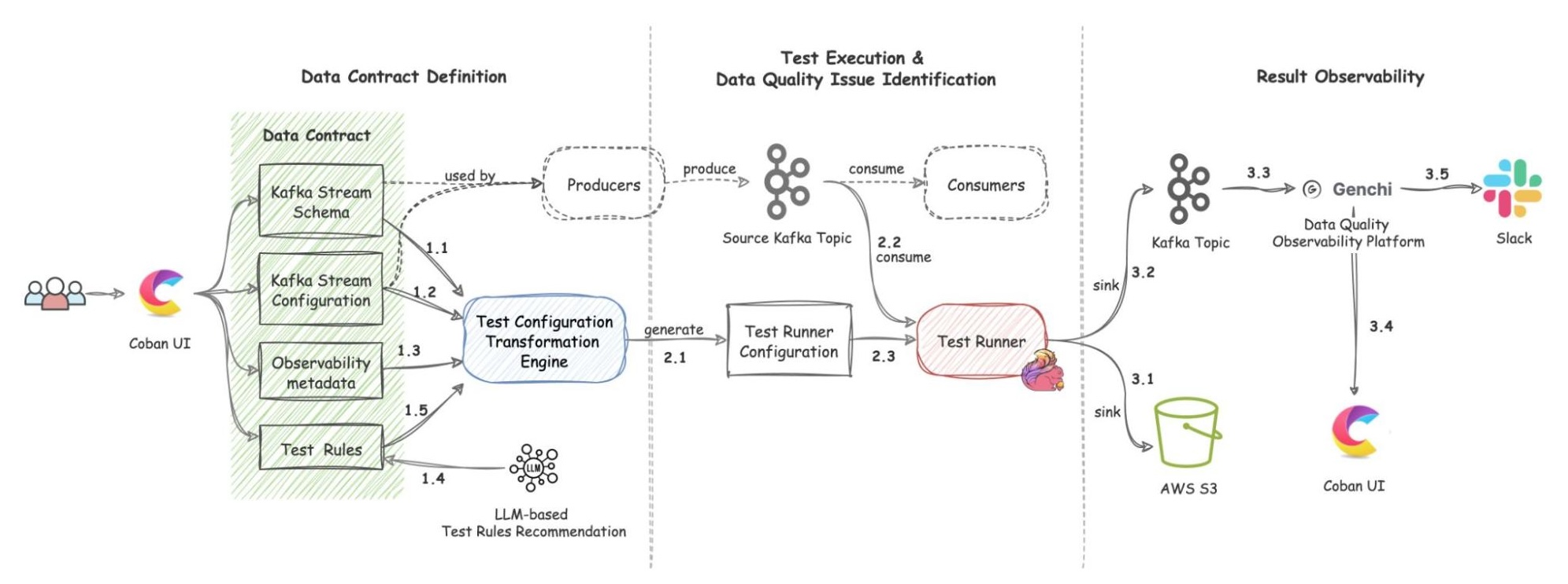

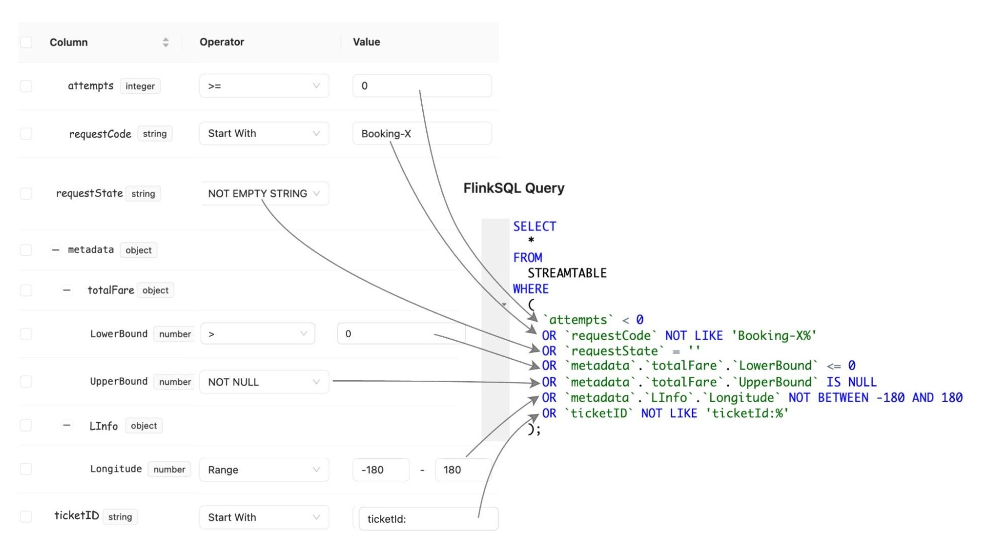
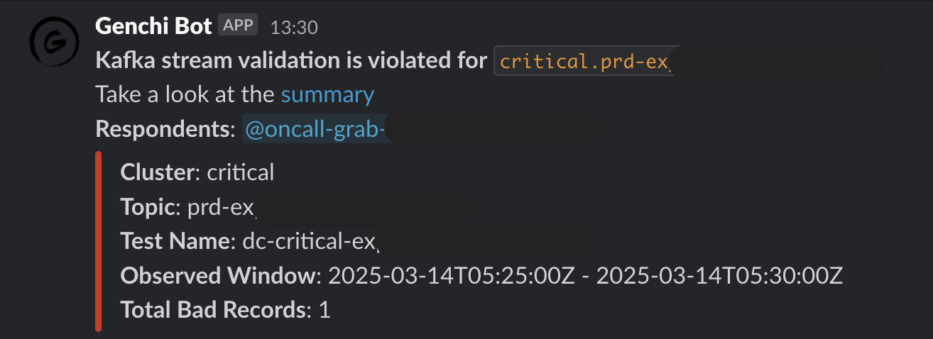
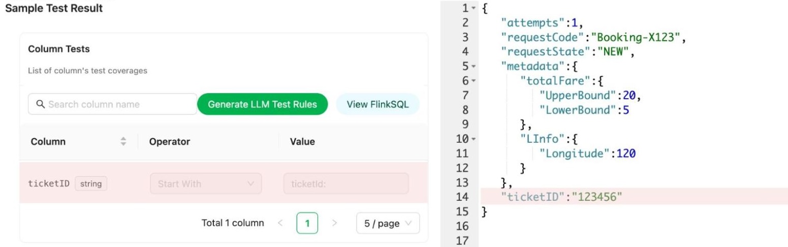

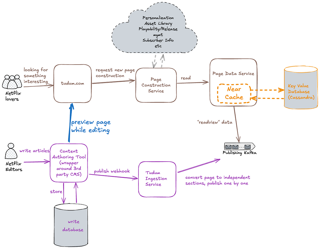
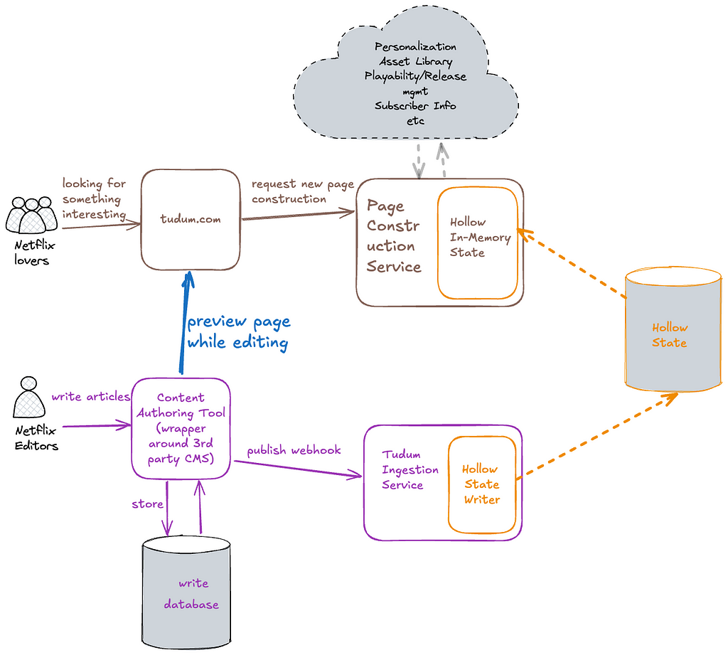
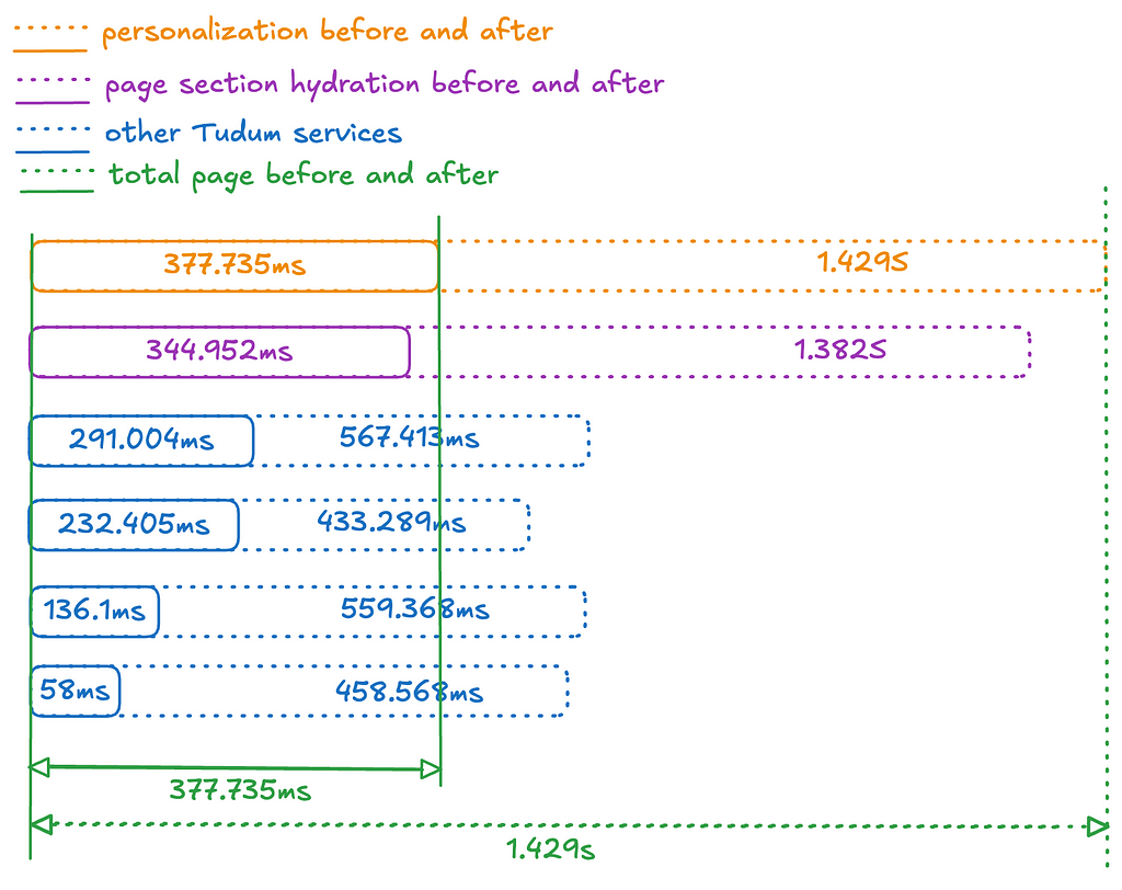


 Tarun Rai Madan is a Principal Product Manager at Amazon Web Services (AWS). He specializes in serverless technologies and leads product strategy to help customers achieve accelerated business outcomes with event-driven applications, using services like AWS Lambda, AWS Step Functions, Apache Kafka, and Amazon SQS/SNS. Prior to AWS, he was an engineering leader in the semiconductor industry, and led development of high-performance processors for wireless, automotive, and data center applications.
 Masudur Rahaman Sayem is a Streaming Data Architect at AWS with over 25 years of experience in the IT industry. He collaborates with AWS customers worldwide to architect and implement sophisticated data streaming solutions that address complex business challenges. As an expert in distributed computing, Sayem specializes in designing large-scale distributed systems architecture for maximum performance and scalability. He has a keen interest and passion for distributed architecture, which he applies to designing enterprise-grade solutions at internet scale.


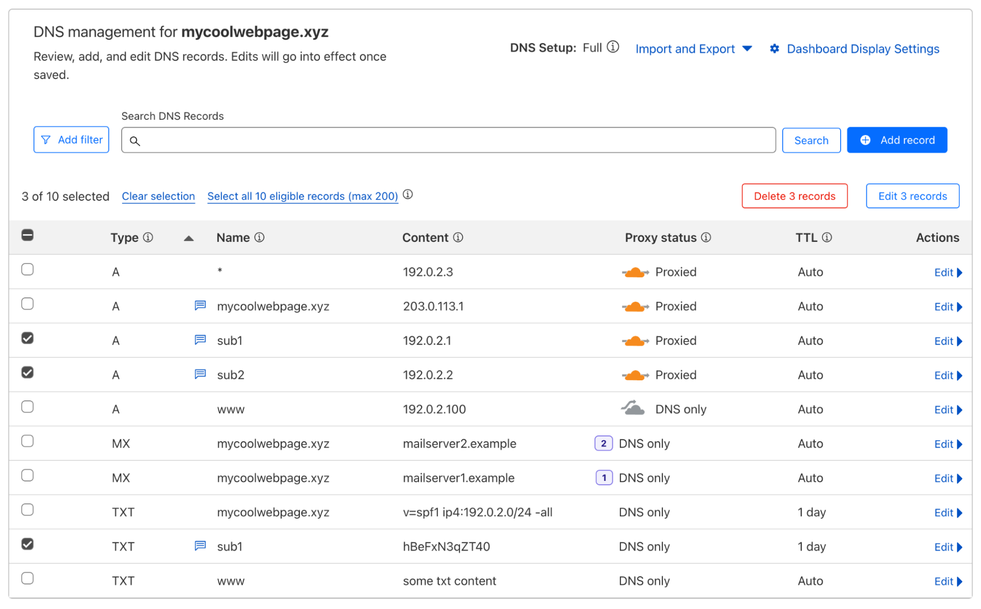


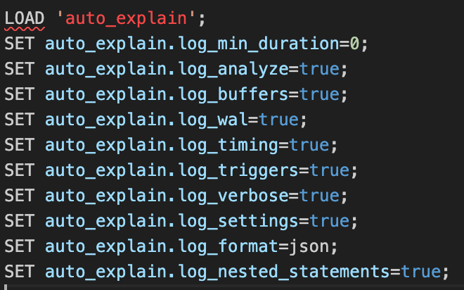


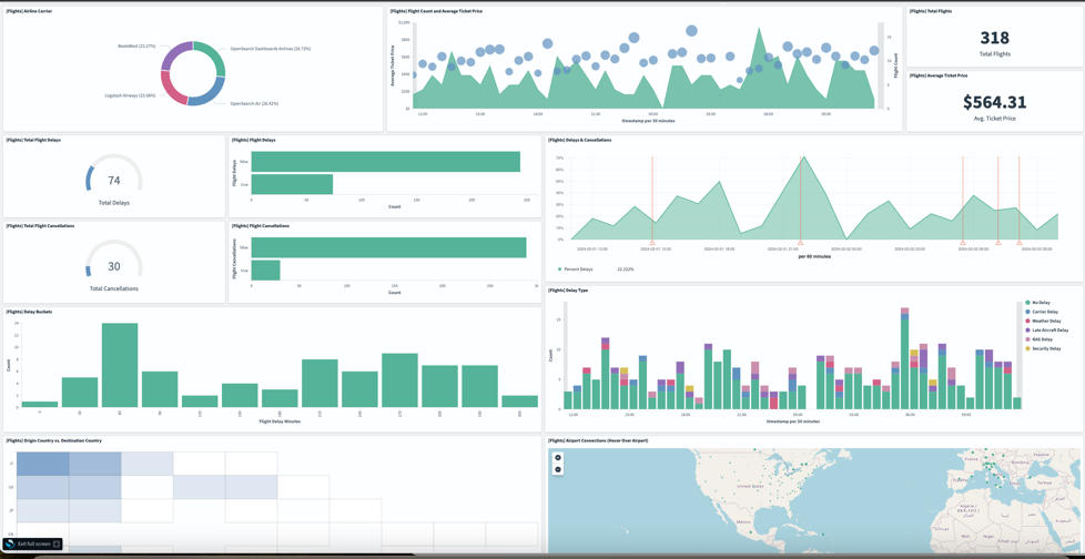
 Ayush Agrawal is a Startups Solutions Architect from Gurugram, India with 11 years of experience in Cloud Computing. With a keen interest in AI, ML, and Cloud Security, Ayush is dedicated to helping startups navigate and solve complex architectural challenges. His passion for technology drives him to constantly explore new tools and innovations. When he’s not architecting solutions, you’ll find Ayush diving into the latest tech trends, always eager to push the boundaries of what’s possible.
 Fraser Sequeira is a Solutions Architect with AWS based in Mumbai, India. In his role at AWS, Fraser works closely with startups to design and build cloud-native solutions on AWS, with a focus on analytics and streaming workloads. With over 10 years of experience in cloud computing, Fraser has deep expertise in big data, real-time analytics, and building event-driven architecture on AWS.
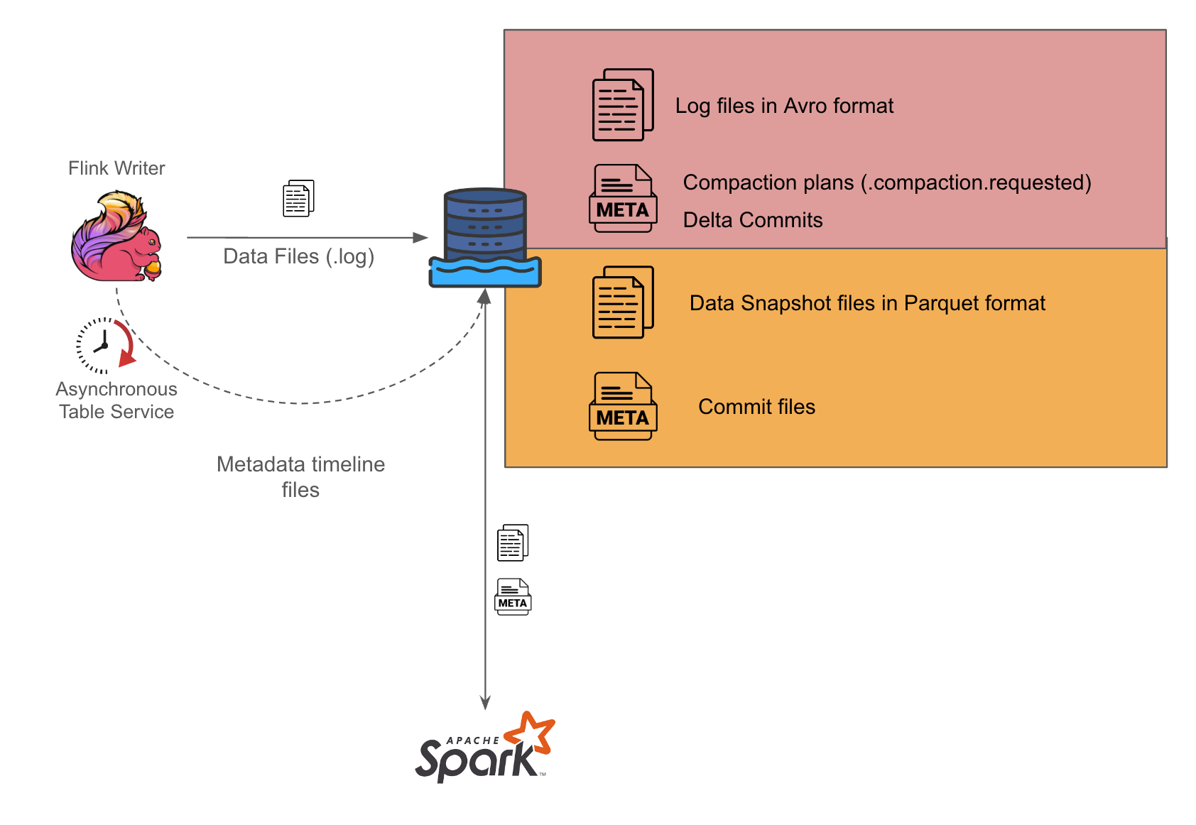
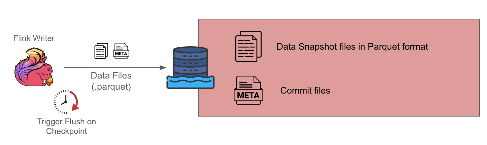
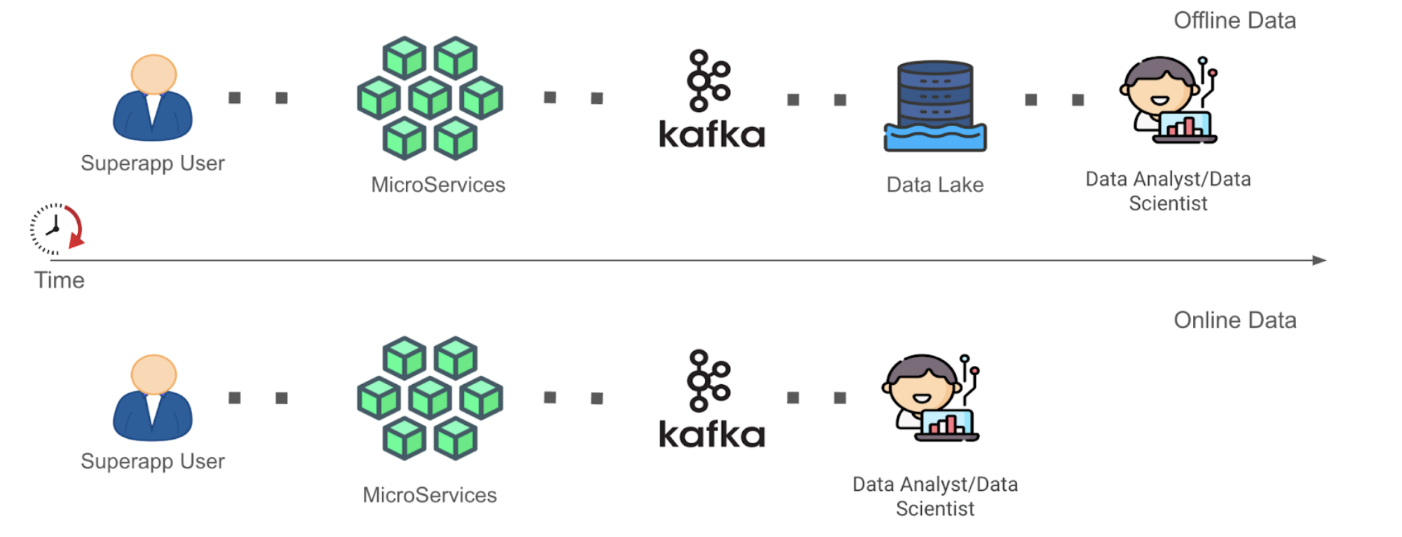
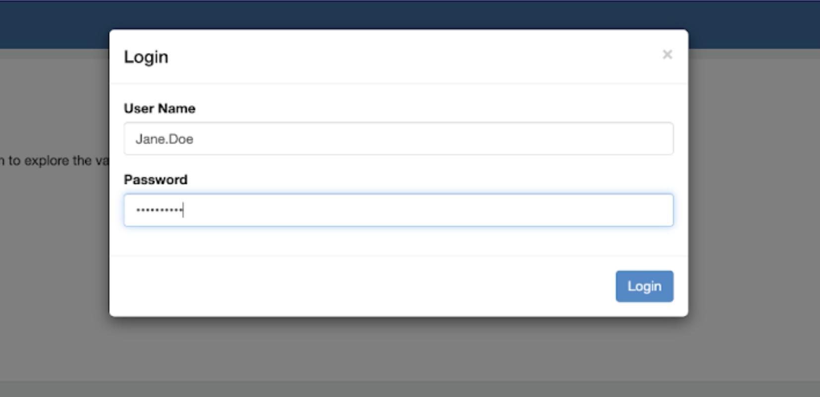
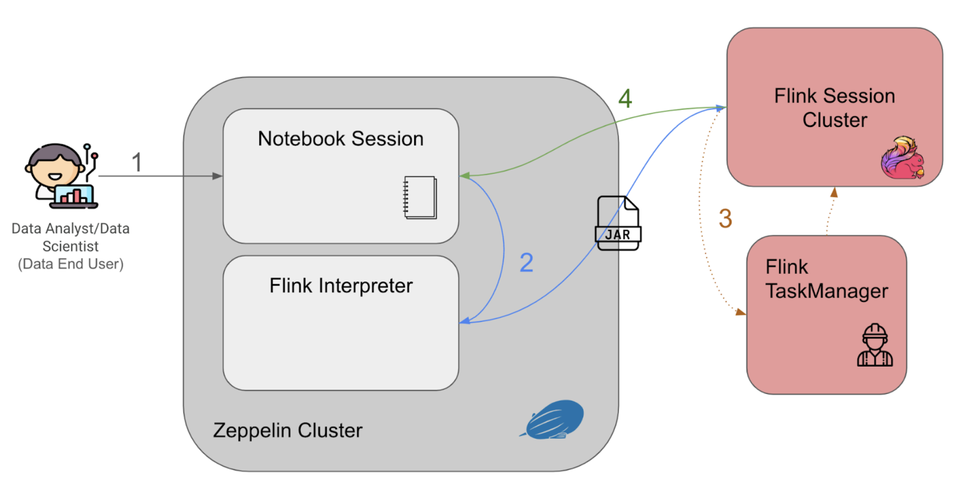
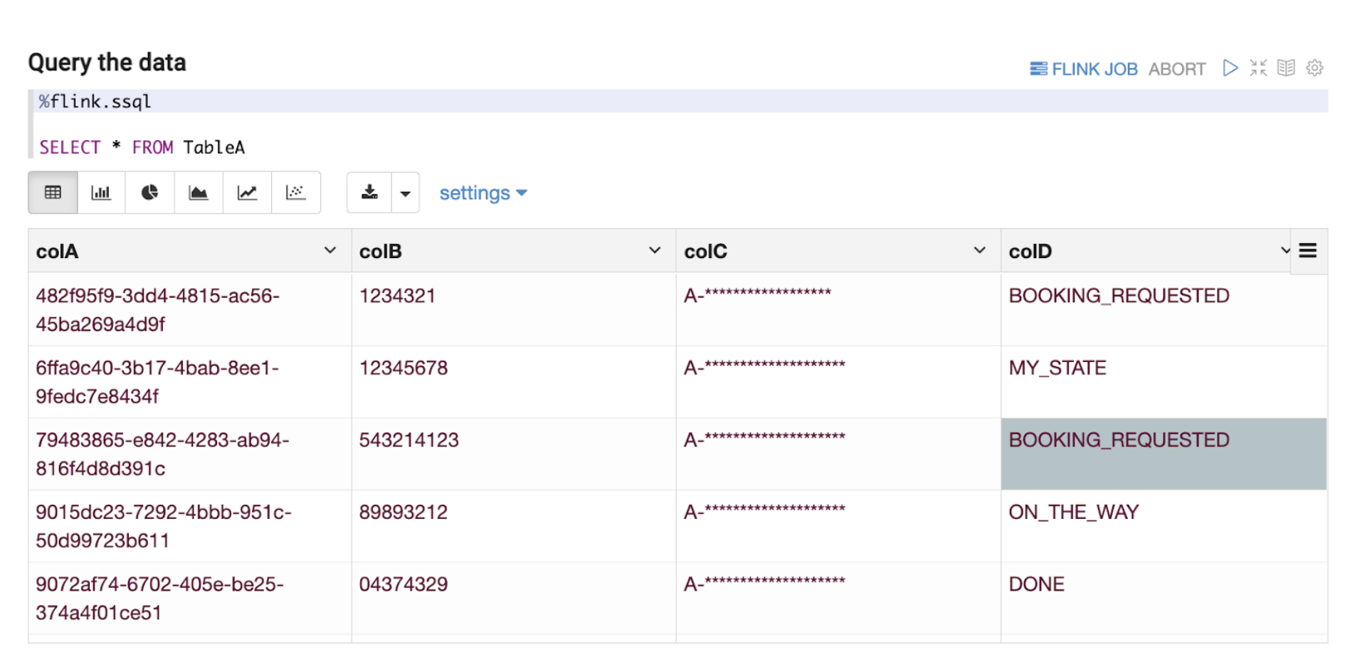
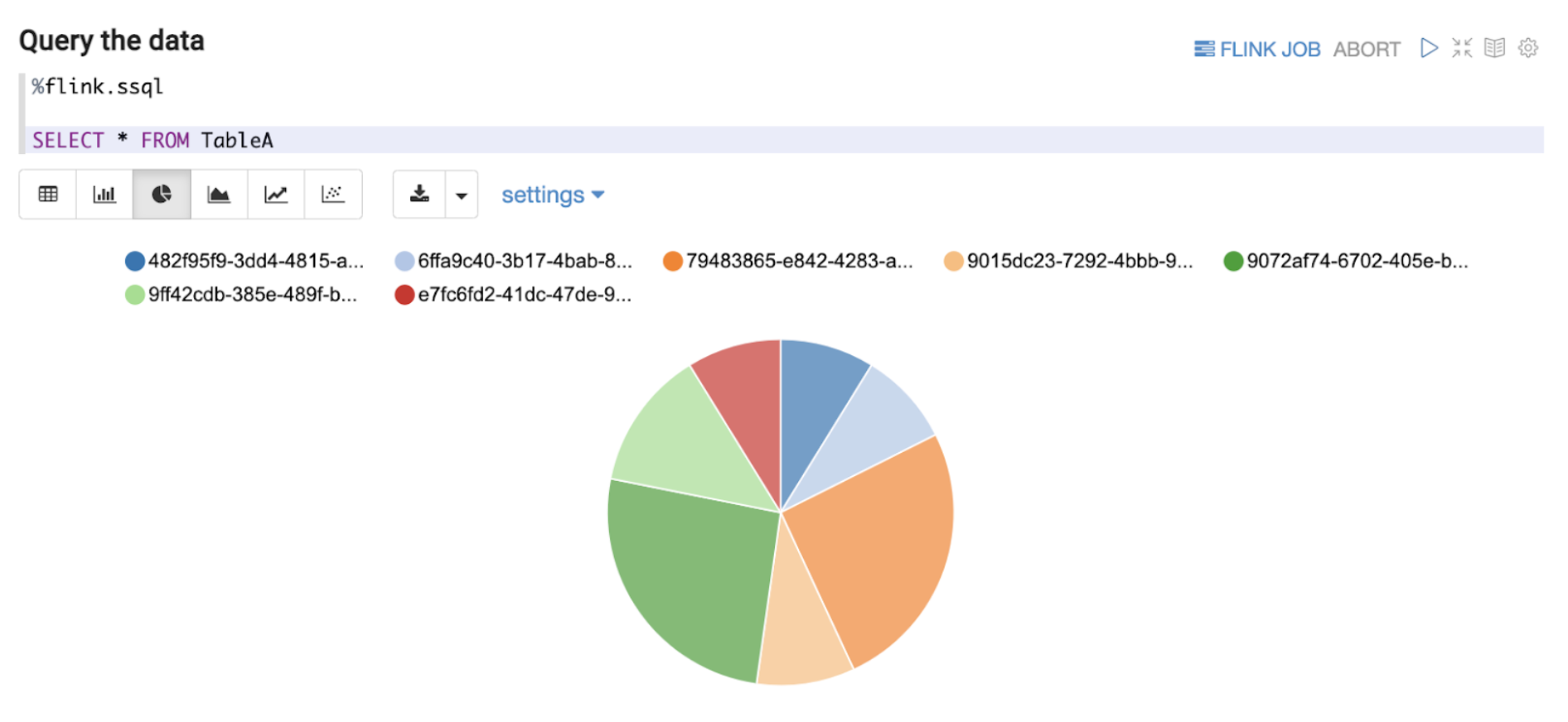
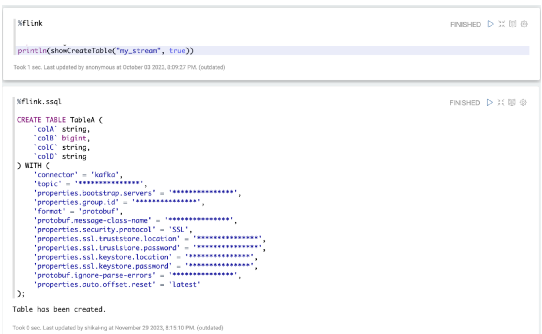
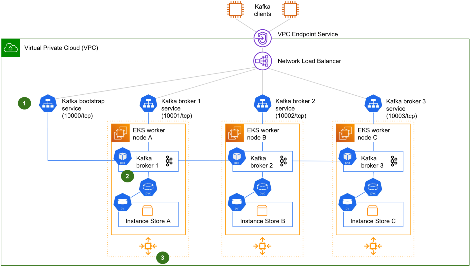
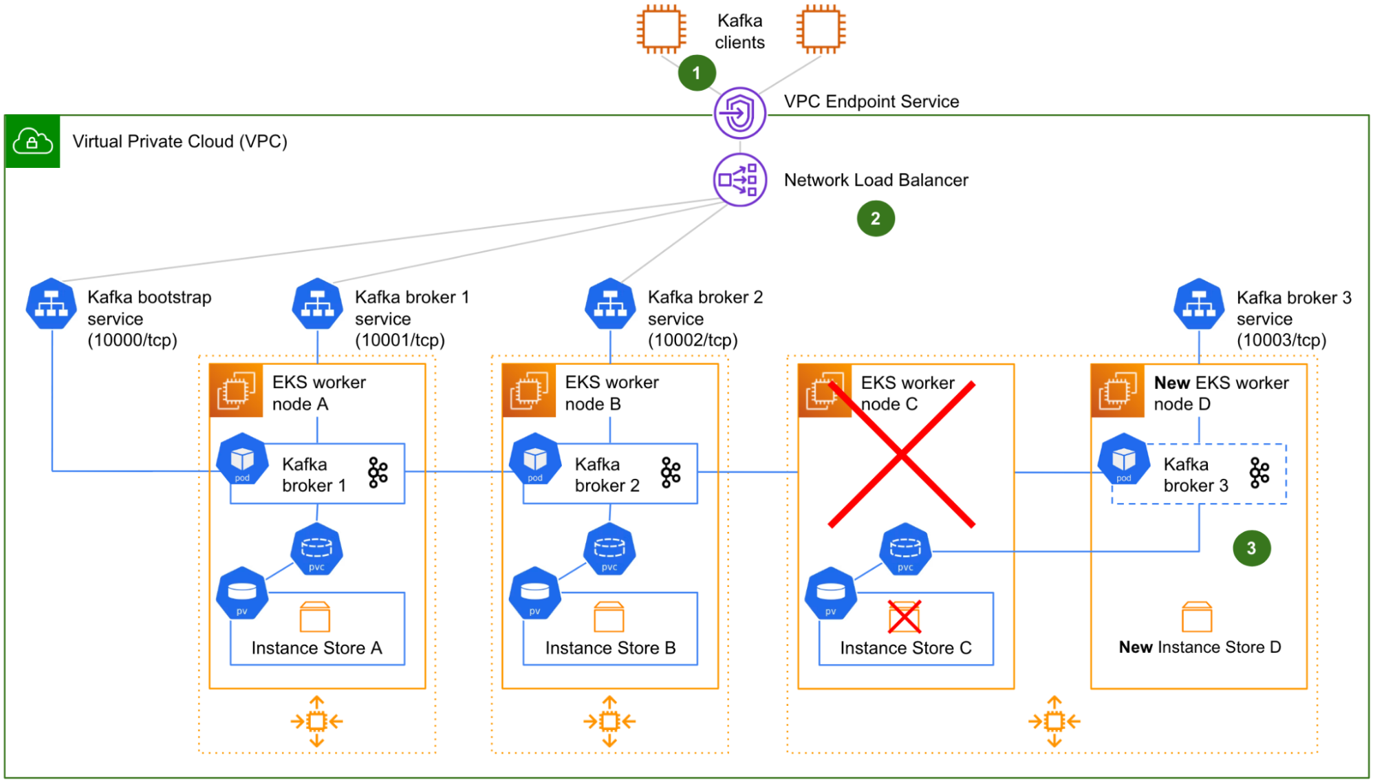
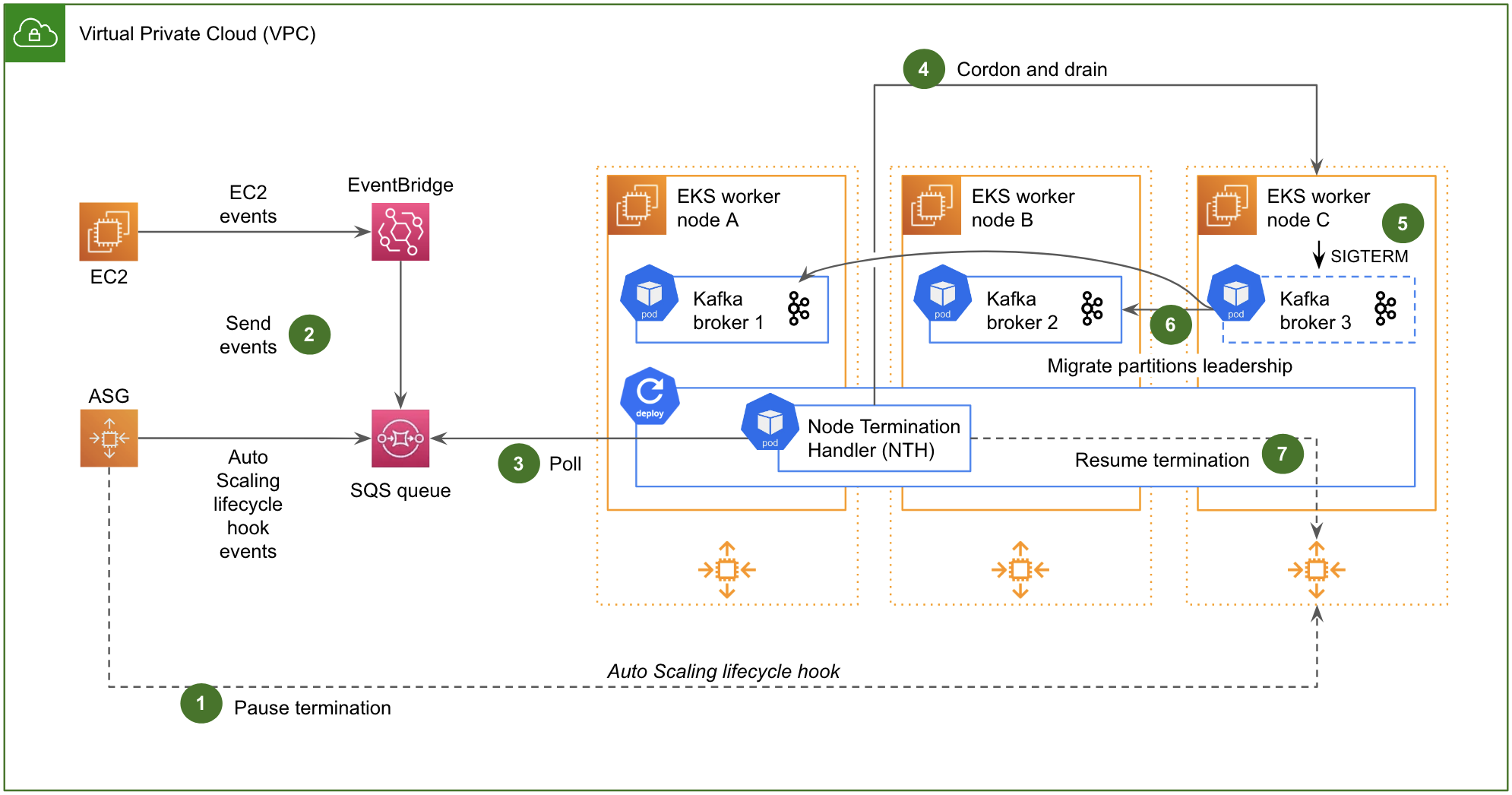
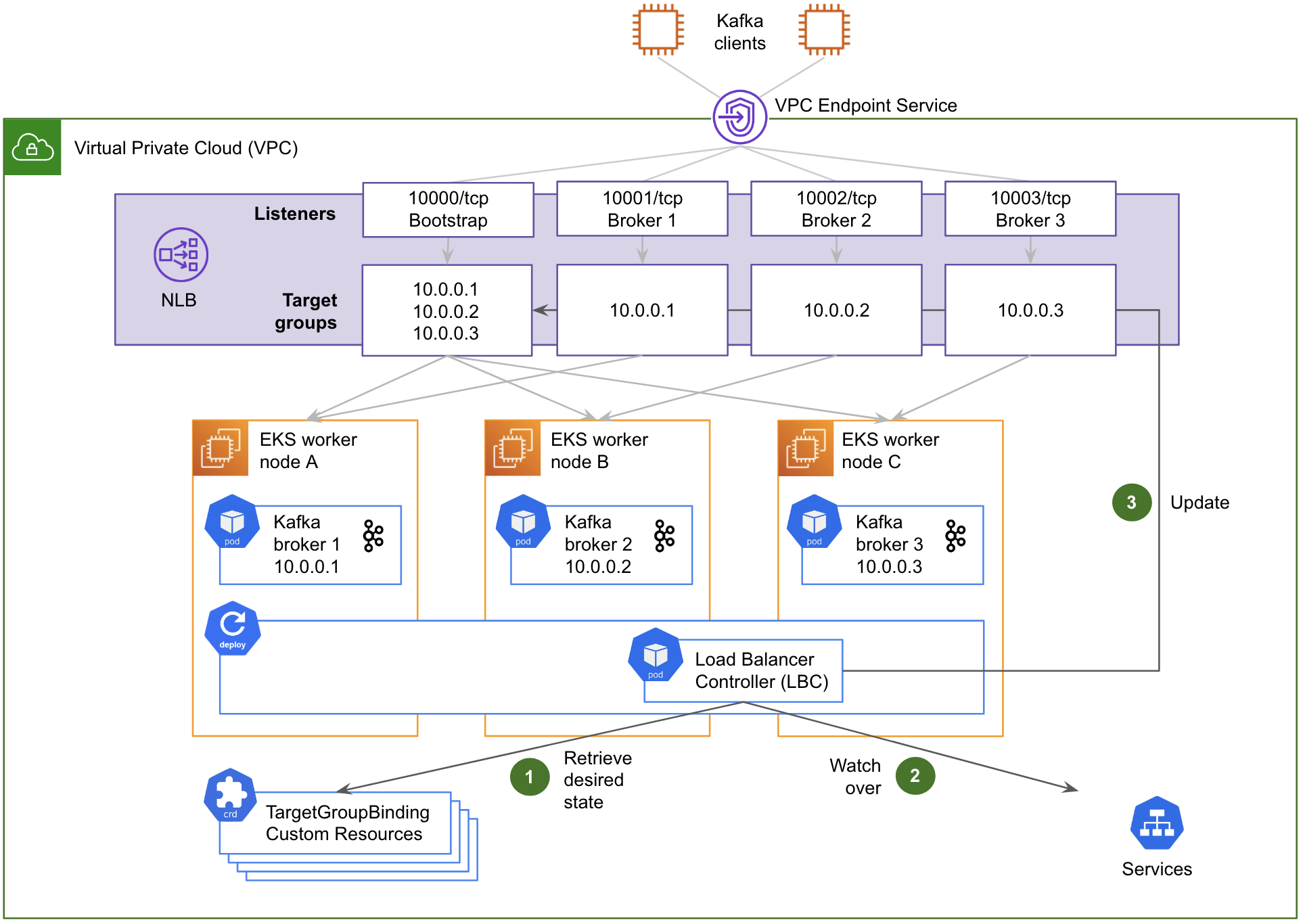
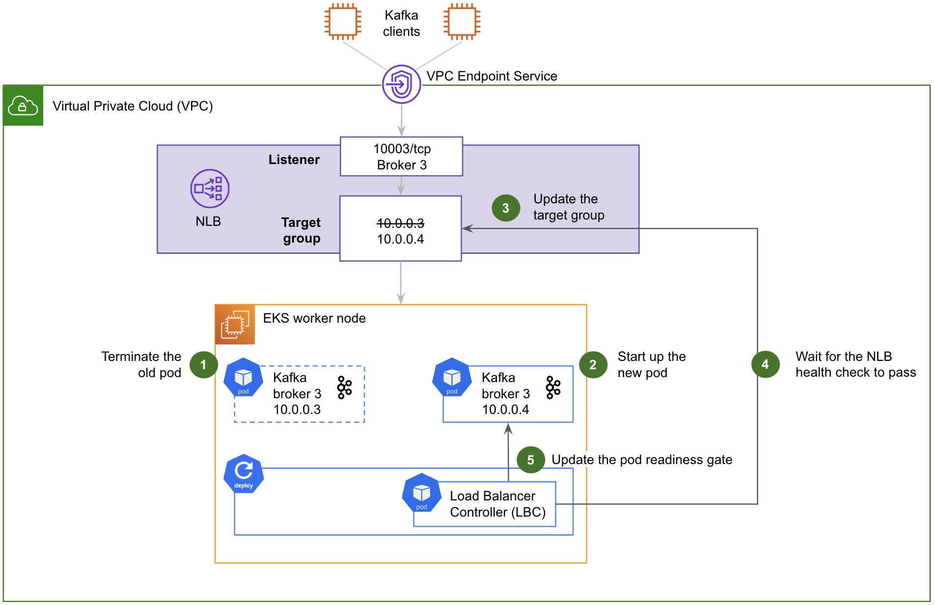
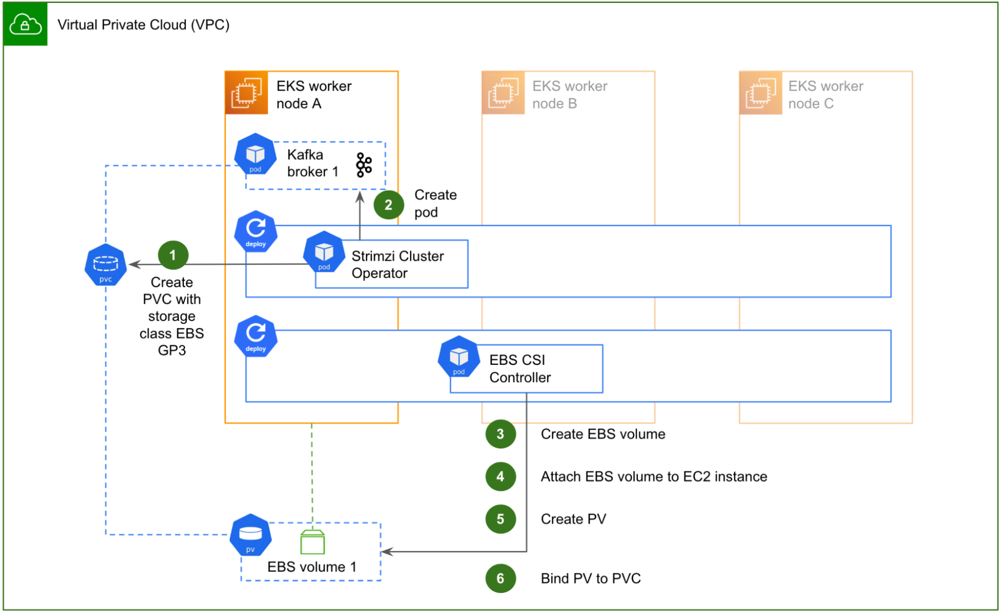
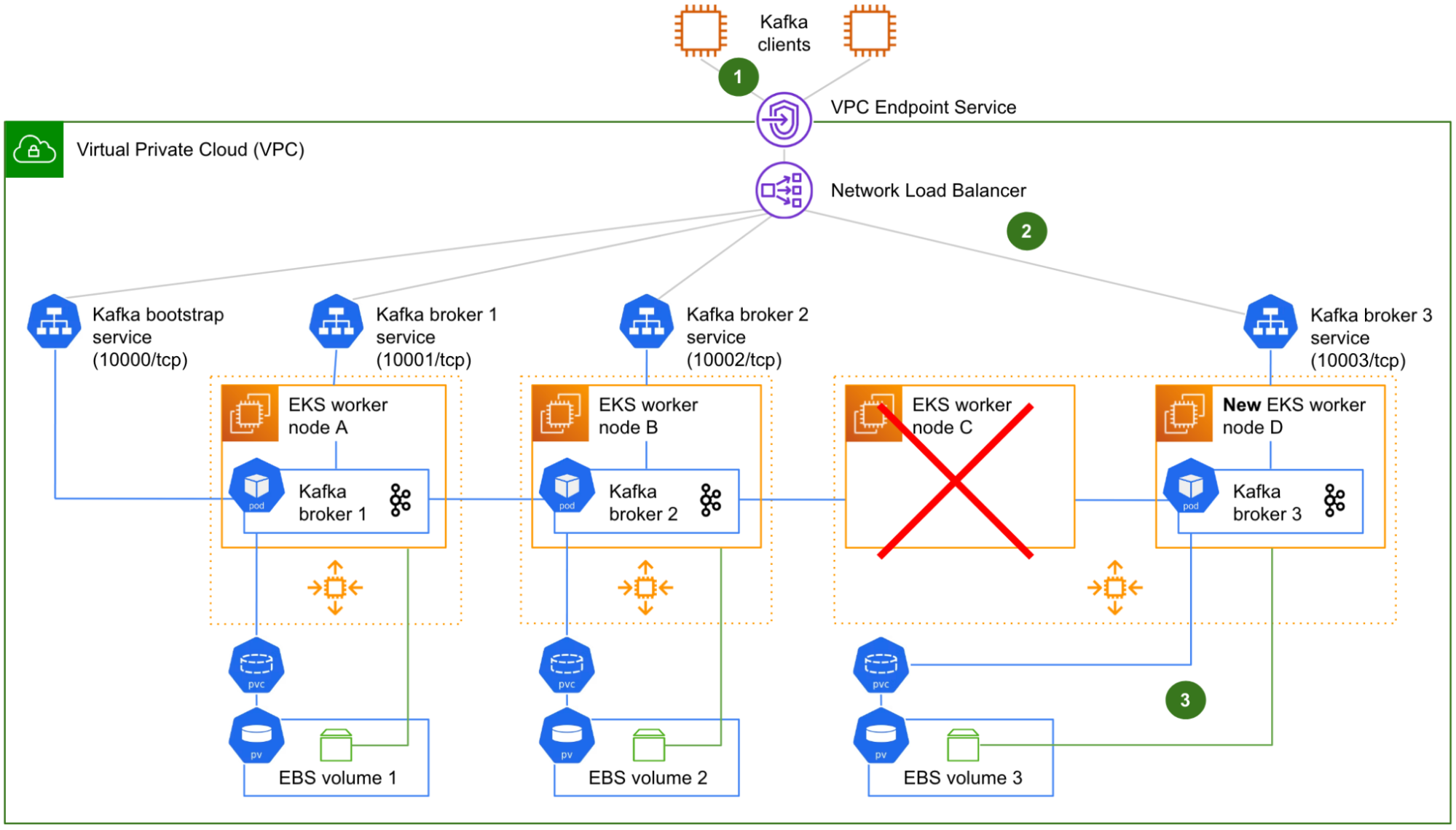

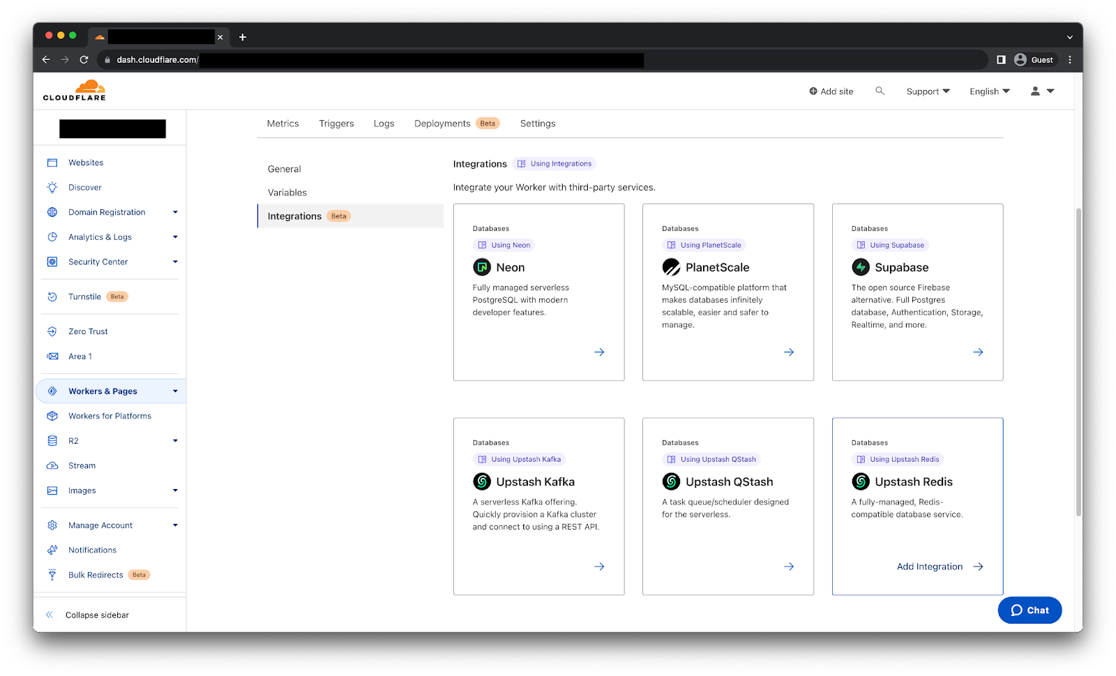
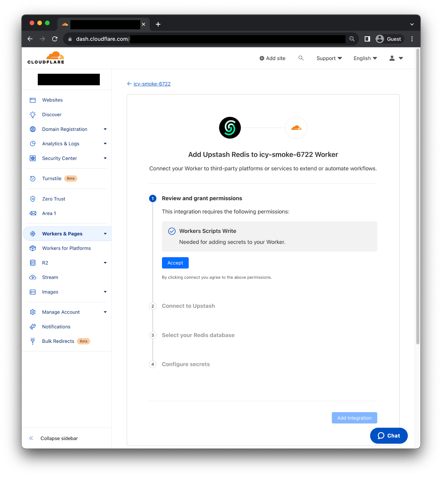
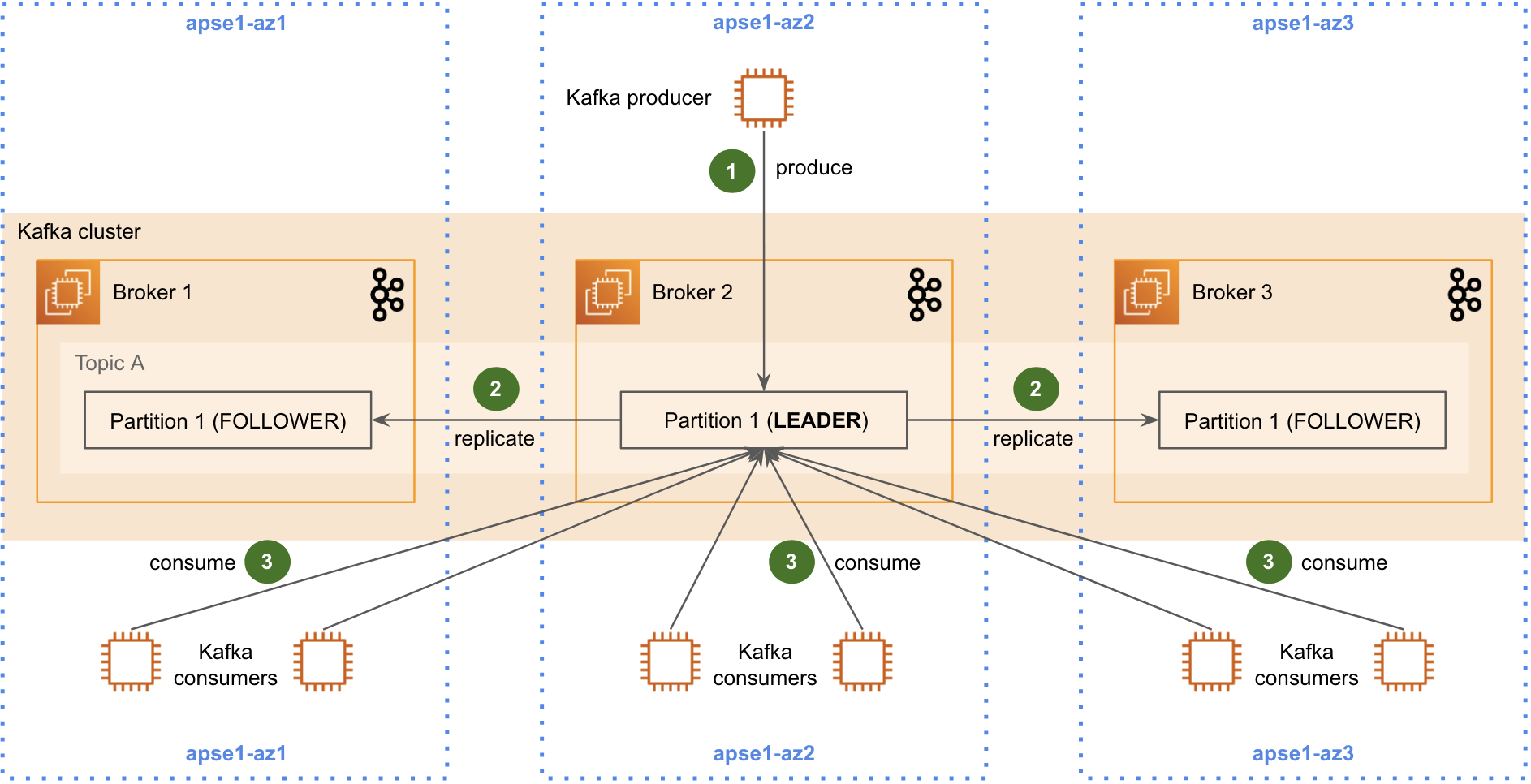
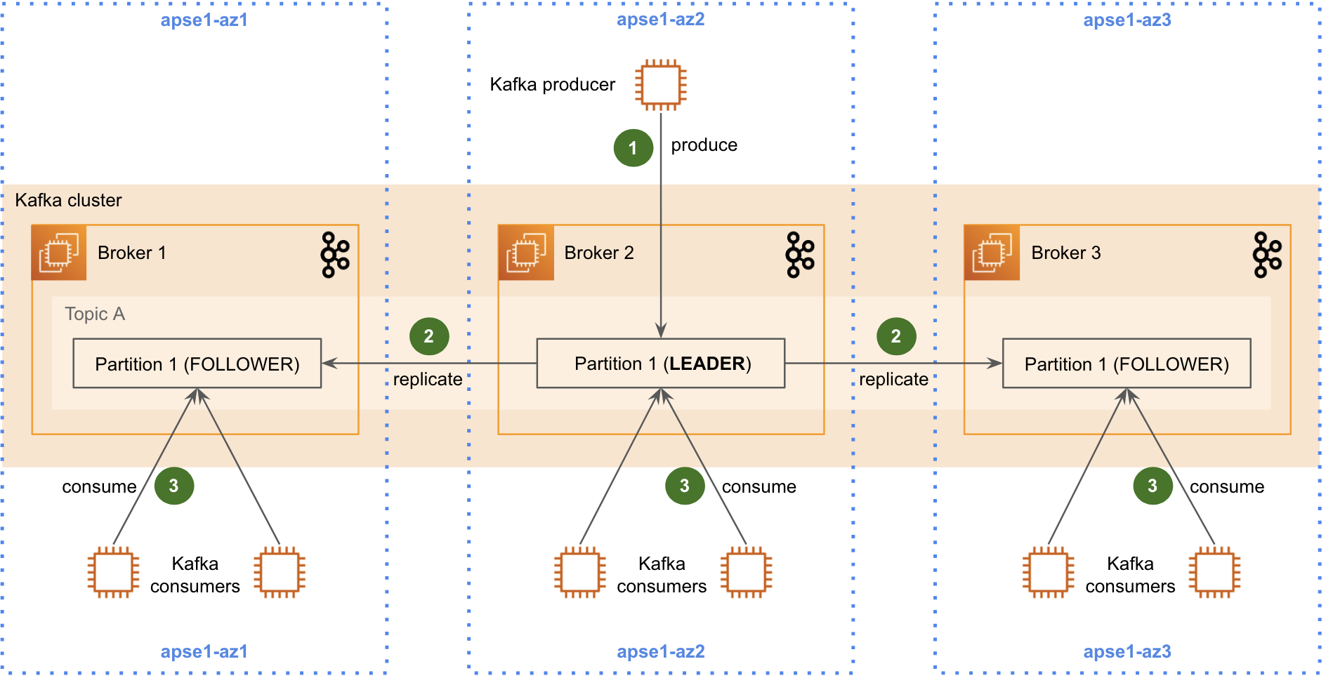
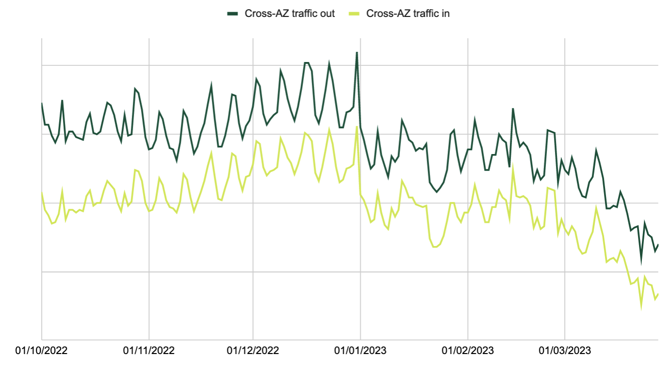
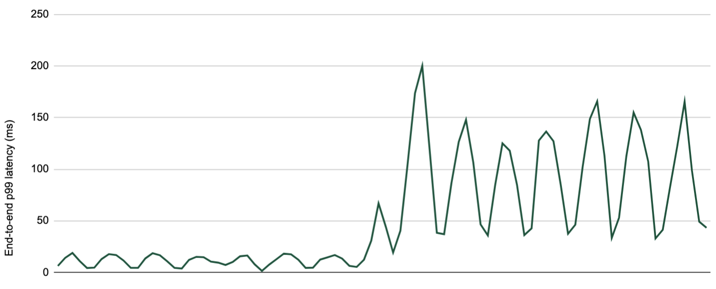
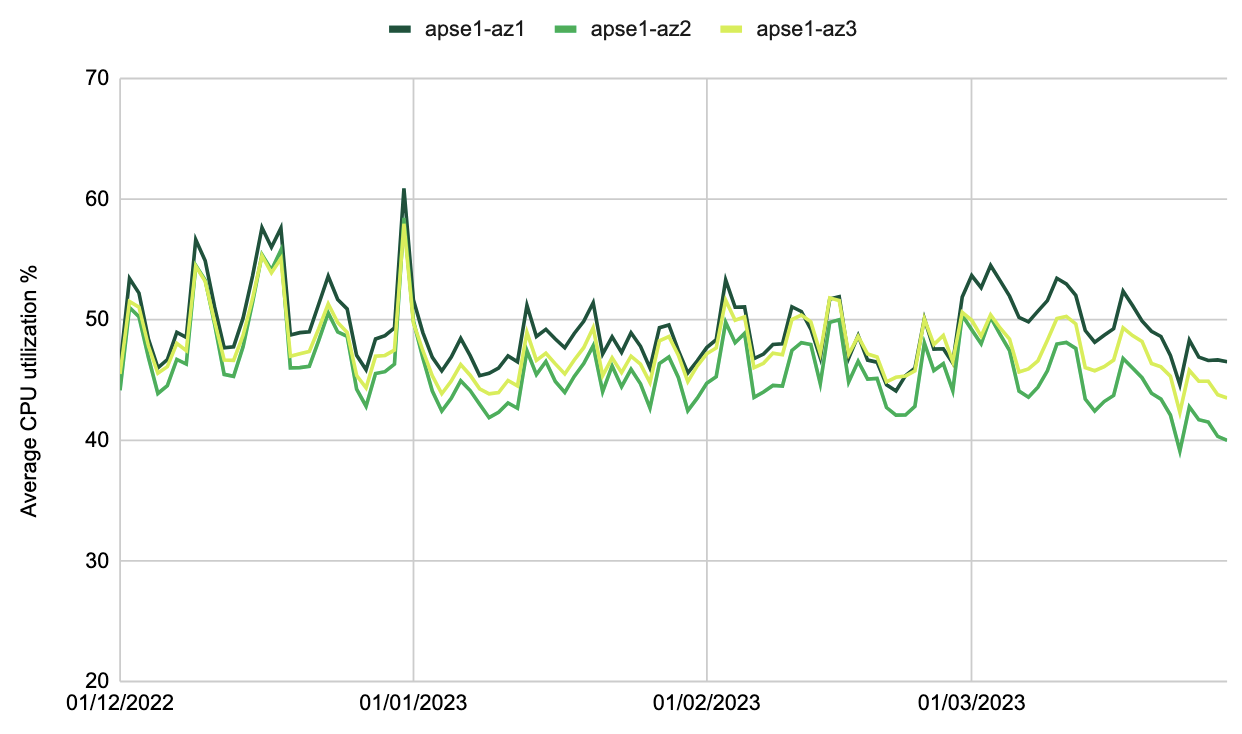


 Nagarjuna Koduru is a Principal Engineer in AWS, currently working for AWS Managed Streaming For Kafka (MSK). He led the teams that built MSK Serverless and MSK Tiered storage products. He previously led the team in Amazon JustWalkOut (JWO) that is responsible for realtime tracking of shopper locations in the store. He played pivotal role in scaling the stateful stream processing infrastructure to support larger store formats and reducing the overall cost of the system. He has keen interest in stream processing, messaging and distributed storage infrastructure.
 Masudur Rahaman Sayem is a Streaming Data Architect at AWS. He works with AWS customers globally to design and build data streaming architectures to solve real-world business problems. He specializes in optimizing solutions that use streaming data services and NoSQL. Sayem is very passionate about distributed computing.
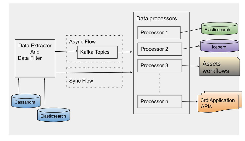


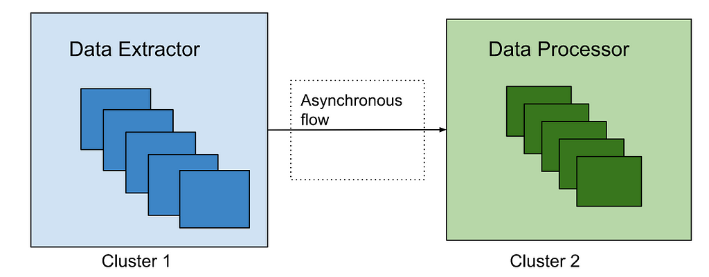
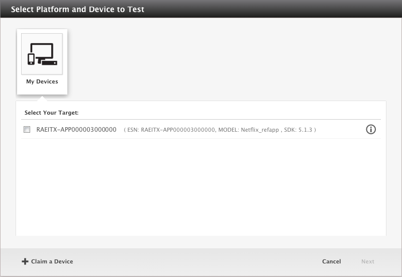

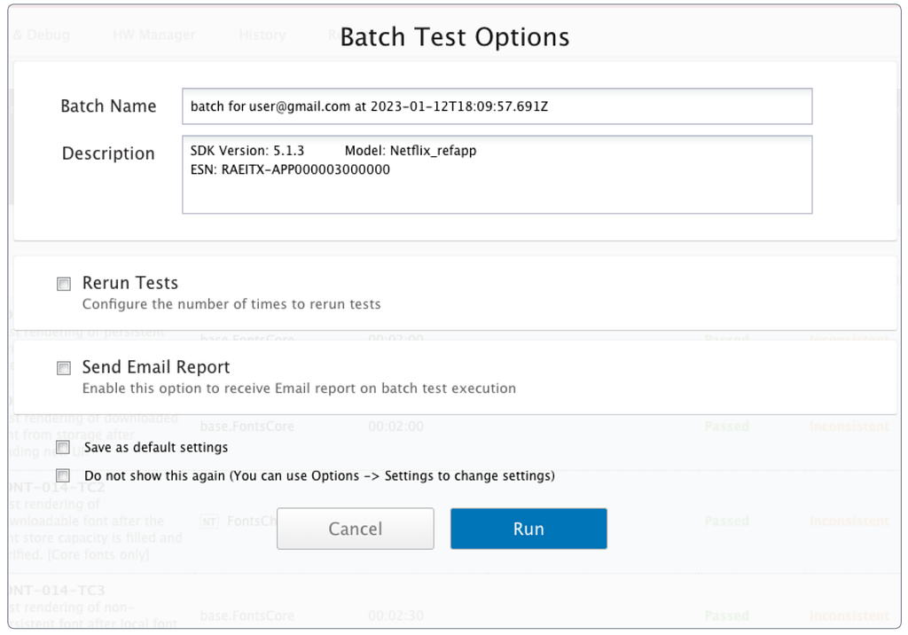
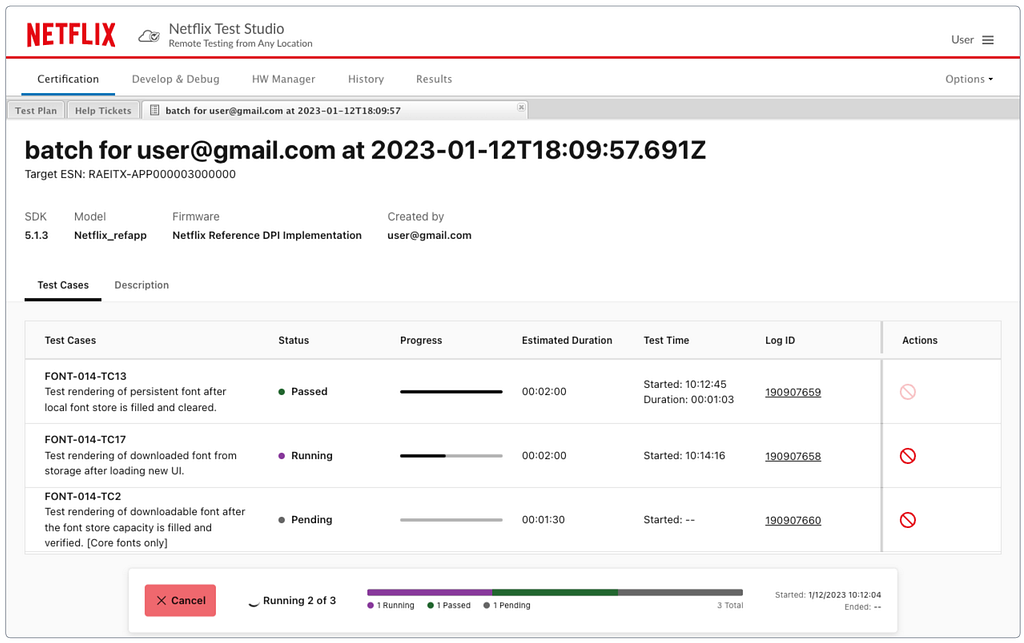
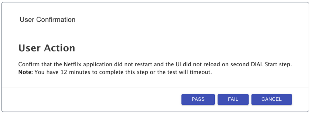
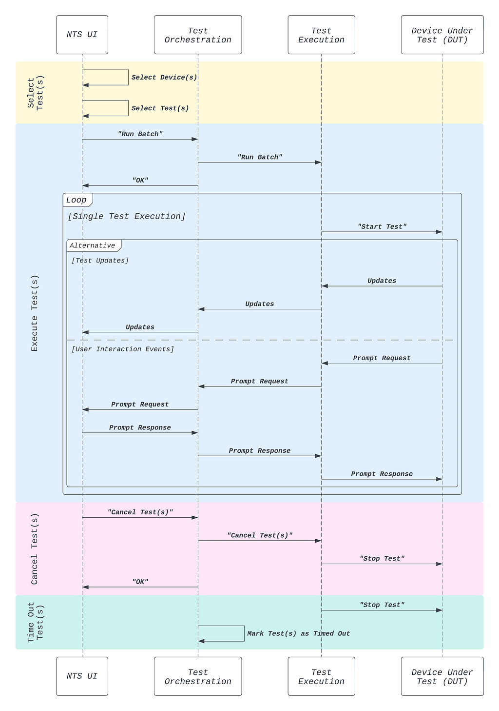
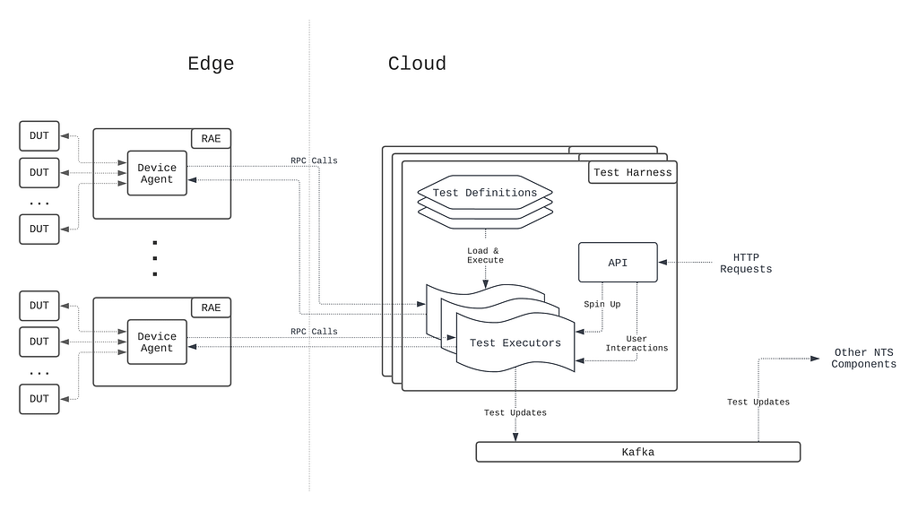


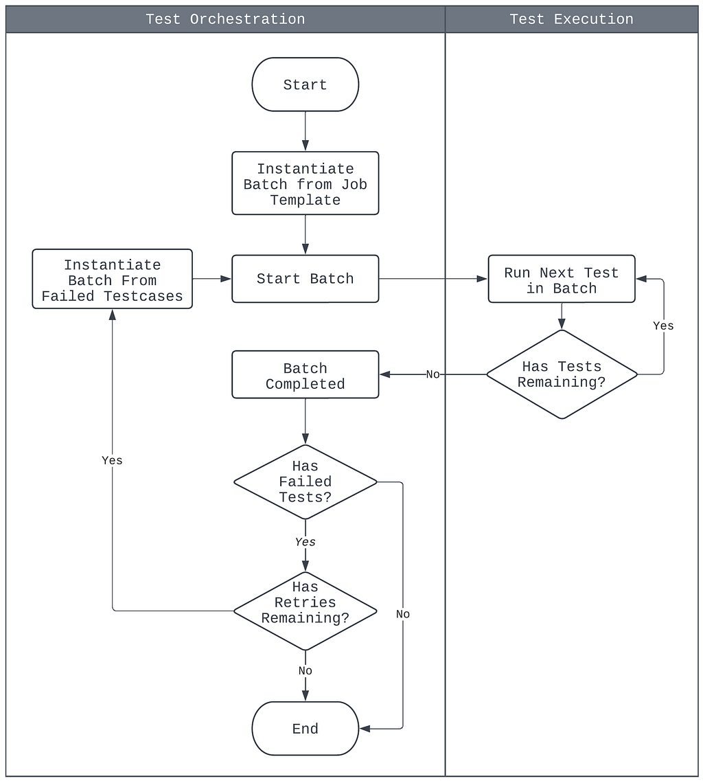


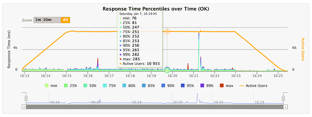


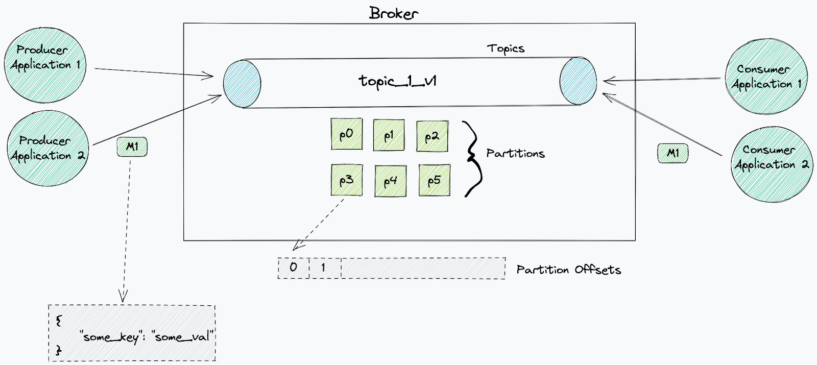
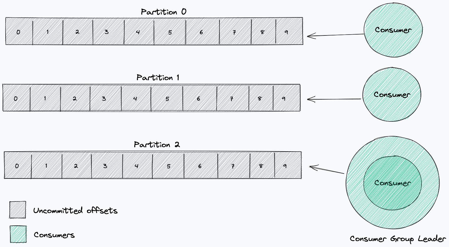
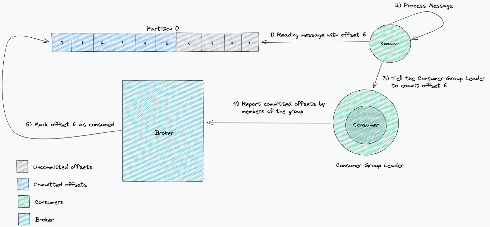
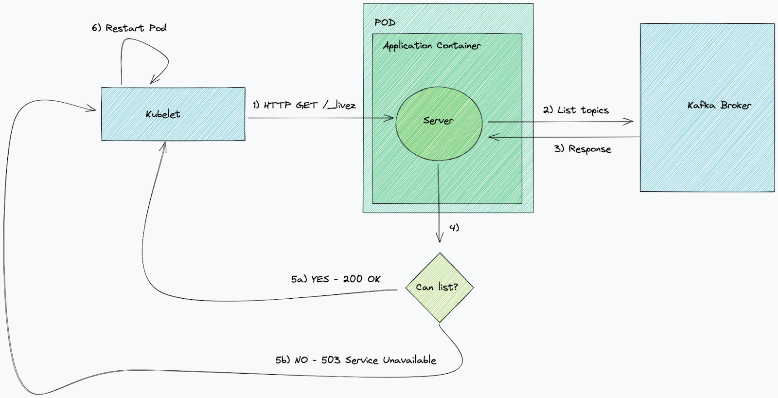
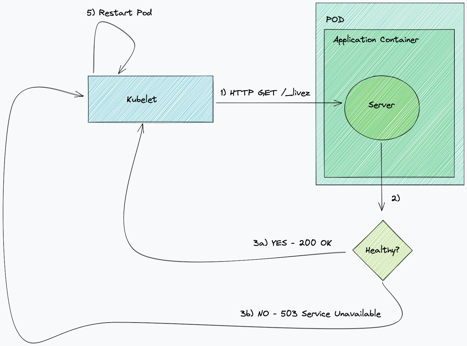
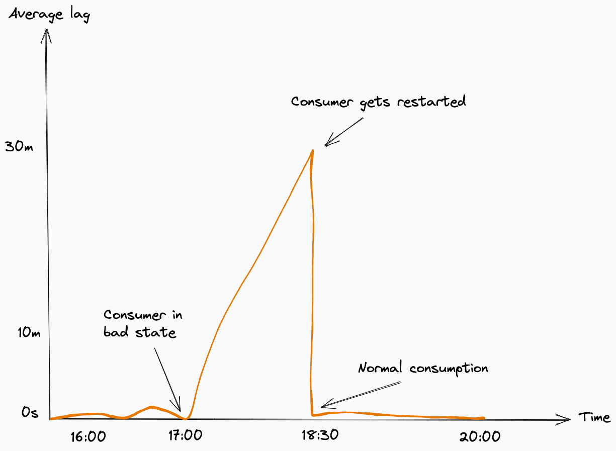
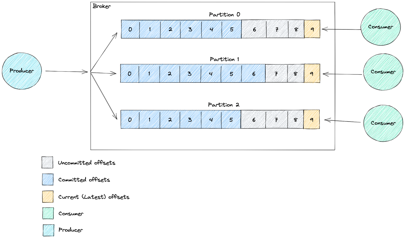
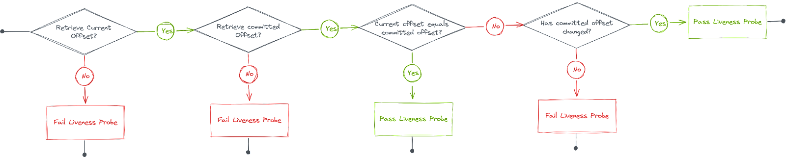
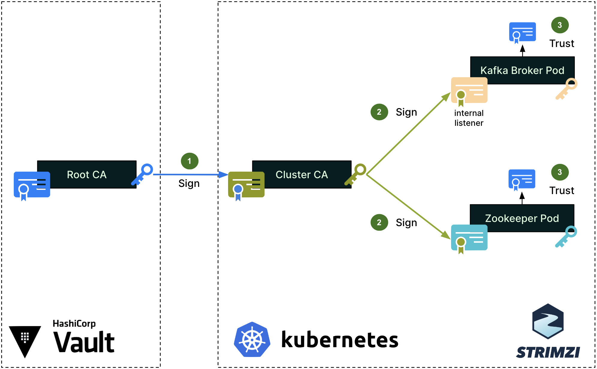
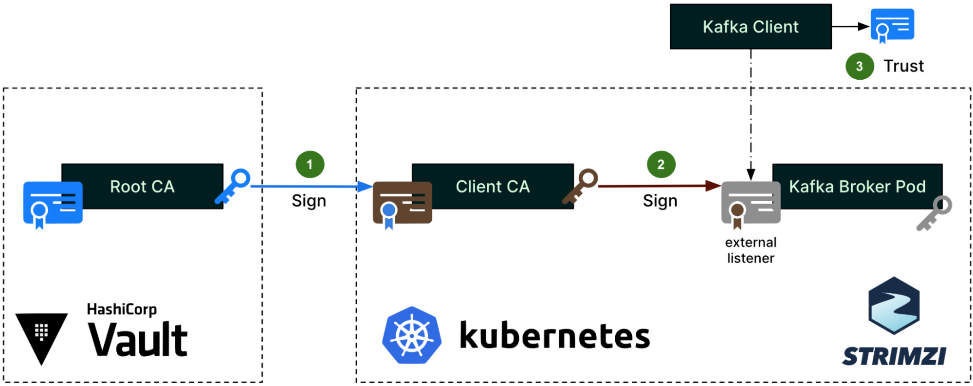
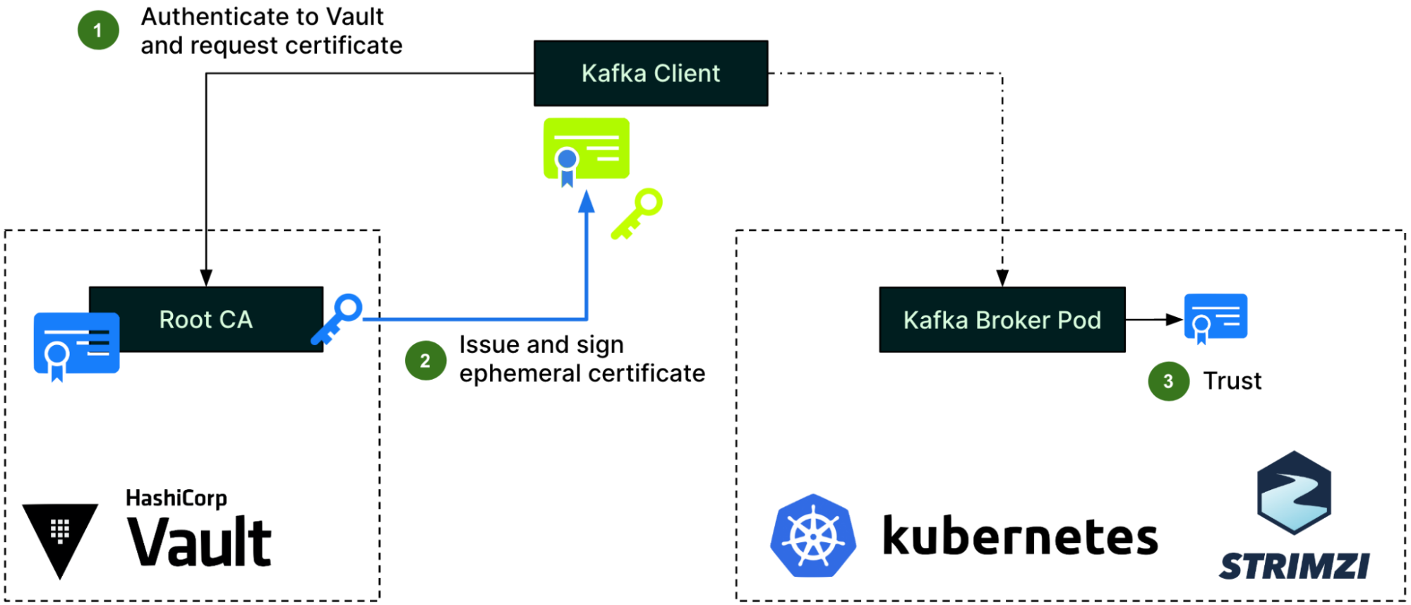
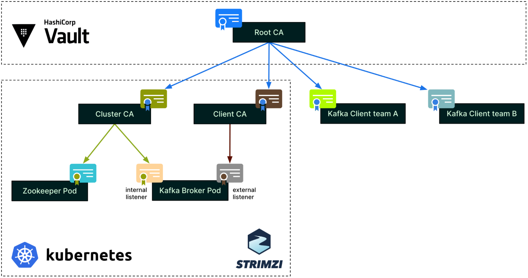
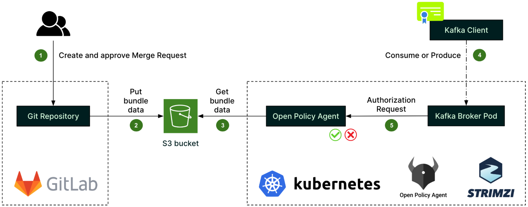


 Tanner Pratt is a Practice Manager at Amazon Web Services. Tanner is leading a team of consultants focusing on Amazon streaming services like Managed Streaming for Apache Kafka, Kinesis Data Streams/Firehose and Kinesis Data Analytics.
 Ed Berezitsky is a Senior Data Architect at Amazon Web Services.Ed helps customers design and implement solutions using streaming technologies, and specializes on Amazon MSK and Apache Kafka.