Tag Archives: SIMD

Optimizing Recommendation Systems with JDK’s Vector API

Post Syndicated from Netflix Technology Blog original https://netflixtechblog.com/optimizing-recommendation-systems-with-jdks-vector-api-30d2830401ec

By Harshad Sane

Ranker is one of the largest and most complex services at Netflix. Among many things, it powers the personalized rows you see on the Netflix homepage, and runs at an enormous scale. When we looked at CPU profiles for this service, one feature kept standing out: video serendipity scoring — the logic that answers a simple question:

“How different is this new title from what you’ve been watching so far?”

This single feature was consuming about 7.5% of total CPU on each node running the service. What started as a simple idea — “just batch the video scoring feature” — turned into a deeper optimization journey. Along the way we introduced batching, re-architected memory layout and tried various libraries to handle the scoring kernels.

Read on to learn how we achieved the same serendipity scores, but at a meaningfully lower CPU per request, resulting in a reduced cluster footprint.

Problem: The Hotspot in Ranker

At a high level, serendipity scoring works like this: A candidate title and each item in a member’s viewing history are represented as embeddings in a vector space. For each candidate, we compute its similarity against the history embeddings, find the maximum similarity, and convert that into a “novelty” score. That score becomes an input feature to the downstream recommendation logic.

The original implementation was straightforward but expensive. For each candidate we fetch its embedding, loop over the history to compute cosine similarity one pair at a time and track the maximum similarity score. Although it is easy to reason about, at Ranker’s scale, this results in significant sequential work, repeated embedding lookups, scattered memory access, and poor cache locality. Profiling confirmed this.
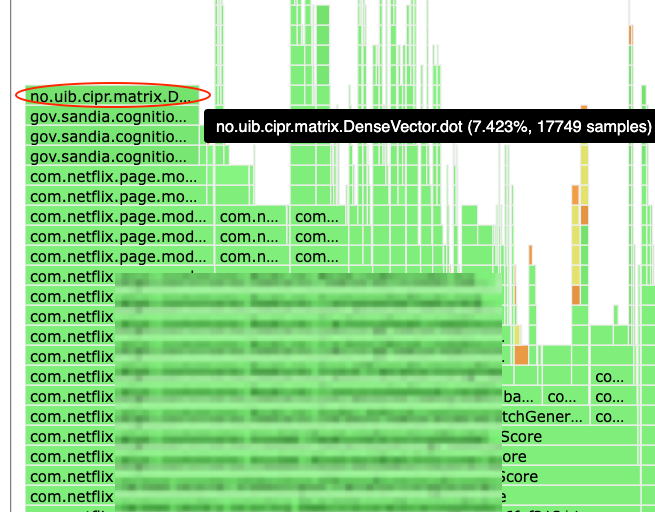
Flamegraph showing inefficient scoring

A flamegraph made it clear: One of the top hotspots in the service was Java dot products inside the serendipity encoder. Algorithmically, the hotspot was a nested loop structure of M candidates × N history items where each pair generates its own cosine similarity i.e. O(M×N) separate dot product operations.

Solution

The Original Implementation: Single video cosine loop

In simplified form the code looked like this:

for (Video candidate : candidates) {
Vector c = embedding(candidate); // D-dimensional
double maxSim = -1.0;

for (Video h : history) {
Vector v = embedding(h); // D-dimensional
double sim = cosine(c, v); // dot(c, v) / (||c|| * ||v||)
maxSim = Math.max(maxSim, sim);
}

double serendipity = 1.0 - maxSim;
emitFeature(candidate, serendipity);
}

The nested for loop with O(M×N) separate dot products brought upon its own overheads. One interesting detail we learned by instrumenting traffic shapes: most requests (about 98%) were single-video, but the remaining 2% were large batch requests. Because those batches were so large, the total volume of videos processed ended up being roughly 50:50 between single and batch jobs. This made batching worth pursuing even if it didn’t help the median request.

Step 1 : Batching, from Nested Loops to Matrix Multiply

The first idea was to stop thinking in terms of “many small dot products” and instead treat the work as a matrix operation. i.e. For batch candidates, implement a data layout to parallelize the math in a single operation i.e. matrix multiply. If D is the embedding dimension:

  1. Pack all candidate embeddings into a matrix A of shape M x D
  2. Pack all history embeddings into a matrix B of shape N x D
  3. Normalize all rows to unit length.
  4. Compute: cosine similarities as
    [ C = A x B^T ]; where C is an M x N matrix of cosine similarities.

In pseudo‑code:

// Build matrices
double[][] A = new double[M][D]; // candidates
double[][] B = new double[N][D]; // history

for (int i = 0; i < M; i++) {
A[i] = embedding(candidates[i]).toArray();
}
for (int j = 0; j < N; j++) {
B[j] = embedding(history[j]).toArray();
}

// Normalize rows to unit vectors
normalizeRows(A);
normalizeRows(B);

// Compute C = A * B^T
double[][] C = matmul(A, B);
C[i][j] = cosine(candidates[i], history[j])

// Derive serendipity
for (int i = 0; i < M; i++) {
double maxSim = max(C[i][0..N-1]);
double serendipity = 1.0 - maxSim;
emitFeature(candidates[i], serendipity);
}

This turns M×N separate dot products into a single matrix multiply, which is exactly what CPUs and optimized kernels are built for. We integrated this into the existing framework by supporting both, encode()for single videos and batchEncode() for batches, while maintaining backward compatibility. At this point it seemed like we were “done”, but we weren't.

Step 2: When Batching Isn’t Enough

Once we had a batched implementation, we ran canaries and saw something surprising: about a 5% performance regression. The algorithm wasn’t the issue — turning M×N separate dot products into a matrix multiplication is mathematically sound. The problem was the overhead we introduced in the first implementation.

  1. Our initial version built double[][] matrices for candidates, history, and results on every batch. Those large, short-lived allocations created GC pressure, and the double[][] layout itself is non-contiguous in memory, which meant extra pointer chasing and worse cache behavior.
  2. On top of that, the first-cut Java matrix multiply was a straightforward scalar implementation, so it couldn’t take advantage of SIMD. In other words, we paid the cost of batching without getting the compute efficiency we were aiming for.

The lesson was immediate: algorithmic improvements don’t matter if the implementation details—memory layout, allocation strategy, and the compute kernel—work against you. That set up the next step for making the data layout cache-friendly and eliminating per-batch allocations before revisiting the matrix multiply kernel.

Step 3: Flat Buffers & ThreadLocal Reuse

We reworked the data layout to be cache-friendly and allocation-light. Instead of double[m][n], we moved to flat double[] buffers in row-major order. That gave us contiguous memory and predictable access patterns. Then we introduced a ThreadLocal<BufferHolder> that owns reusable buffers for candidates, history, and any other scratch space. Buffers grow as needed but never shrink, which avoids per-request allocation while keeping each thread isolated (no contention). A simplified sketch:

class BufferHolder {  
double[] candidatesFlat = new double[0];
double[] historyFlat = new double[0];

double[] getCandidatesFlat(int required) {
if (candidatesFlat.length < required) {
candidatesFlat = new double[required];
}
return candidatesFlat;
}

double[] getHistoryFlat(int required) {
if (historyFlat.length < required) {
historyFlat = new double[required];
}
return historyFlat;
}
}

private static final ThreadLocal<BufferHolder> threadBuffers =
ThreadLocal.withInitial(BufferHolder::new);

This change alone made the batched path far more predictable: fewer allocations, less GC pressure, and better cache locality.

Now the remaining question was the one we originally thought we were answering: what’s the best way to do the matrix multiply?

Step 4: BLAS: Great in Tests, Not in Production

The obvious next step was BLAS (Basic Linear Algebra Subprograms). In isolation, microbenchmarks looked promising. But once integrated into the real batch scoring path, the gains didn’t materialize. A few things were working against us:

  • The default netlib-java path was using F2J (Fortran-to-Java) BLAS rather than a truly native implementation.
  • Even with native BLAS, we paid overhead for setup and JNI transitions.
  • Java’s row-major layout doesn’t match the column-major expectations of many BLAS routines, which can introduce conversion and temporary buffers.
  • Those extra allocations and copies mattered in the full pipeline, especially alongside TensorFlow embedding work.

BLAS was still a useful experiment — it clarified where time was being spent, but it wasn’t the drop-in win we wanted. What we needed was something that stayed pure Java, fit our flat-buffer architecture, and could still exploit SIMD.

Step 5: JDK Vector API to the rescue

A Short Note on the JDK Vector API: The JDK Vector API is an incubating feature that provides a portable way to express data-parallel operations in Java — think “SIMD without intrinsics”. You write in terms of vectors and lanes, and the JIT maps those operations to the best SIMD instructions available on the host CPU (SSE/AVX2/AVX-512), with a scalar fallback when needed. More crucially for us, it’s pure Java: no native dependencies, no JNI transitions, and a development model that looks like normal Java code rather than platform-specific assembly or intrinsics.

This was a particularly good match for our workload because we had already moved embeddings into flat, contiguous double[] buffers, and the hot loop was dominated by large numbers of dot products. The final step was to replace BLAS with a pure-Java SIMD implementation using the JDK Vector API. By this point we already had the right shape for high performance — batching, flat buffers, and ThreadLocal reuse. So the remaining work was to swap out the compute kernel without introducing JNI overhead or platform-specific code. We did that behind a small factory. At class load time, MatMulFactory selects the best available implementation:

  • If jdk.incubator.vector is available, use a Vector API implementation.
  • Otherwise, fall back to a scalar implementation with a highly optimized loop-unrolled dot product (implemented by my colleague Patrick Strawderman, inspired by patterns used in Lucene)

In the Vector API implementation, the inner loop computes a dot product by accumulating a * b into a vector accumulator using fma() (fused multiply-add). DoubleVector.SPECIES_PREFERRED lets the runtime pick an appropriate lane width for the machine. Here’s a simplified sketch of the inner loop:

// Vector API path (simplified)  
for (int i = 0; i < M; i++) {
for (int j = 0; j < N; j++) {

DoubleVector acc = DoubleVector.zero(SPECIES);
int k = 0;
// SPECIES.length() (e.g. often 4 doubles on AVX2 and 8 doubles on AVX-512).
for (; k + SPECIES.length() <= D; k += SPECIES.length()) {
DoubleVector a = DoubleVector.fromArray(SPECIES, candidatesFlat, i*D + k);
DoubleVector b = DoubleVector.fromArray(SPECIES, historyFlat, j*D + k);
acc = a.fma(b, acc); // fused multiply-add
}
double dot = acc.reduceLanes(VectorOperators.ADD);
// handle tail k..D-1
similaritiesFlat[i*N + j] = dot;
}
}

Figure below shows how the Vector API utilizes SIMD hardware to process multiple doubles per instruction (e.g., 4 lanes on AVX2 and 8 lanes on AVX‑512). What used to be many scalar multiply-adds becomes a smaller number of vector fma() operations plus a reduction—same algorithm, much better use of the CPU’s vector units.
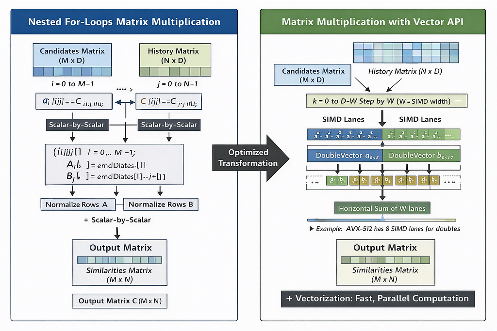
Vectorization with SIMD

Fallbacks & Safety: When the Vector API Isn’t Available

Because the Vector API is still incubating, it requires a runtime flag: –add-modules=jdk.incubator.vector We didn’t want correctness or availability to depend on that flag. So we designed the fallback behavior explicitly: At startup, we detect Vector API support and use the SIMD batched matmul when available; otherwise we fall back to an optimized scalar path, with single-video requests continuing to use the per-item implementation.

That gives us a clean operational story: services can opt in to the Vector API for maximum performance, but the system remains safe and predictable without it.

Results in Production:

With the full design in place with batching, flat buffers, ThreadLocal reuse, and the Vector API, we ran canaries that run production traffic. We observed a ~7% drop in CPU utilization and ~12% drop in average latency. To normalize across any small throughput differences, we also tracked CPU/RPS (CPU consumed per request-per-second). That metric improved by roughly 10%, meaning we could handle the same traffic with about 10% less CPU, and we saw similar numbers hold after full production rollout.
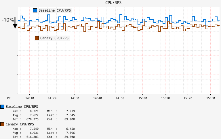
CPU/RPS on Ranker

At the function operator level, we saw the CPU drop from the initial 7.5% to a merely ~1% with the optimization in place. At the assembly level, the shift was clear: from loop-unrolled scalar dot products to a vectorized matrix multiply on AVX-512 hardware.
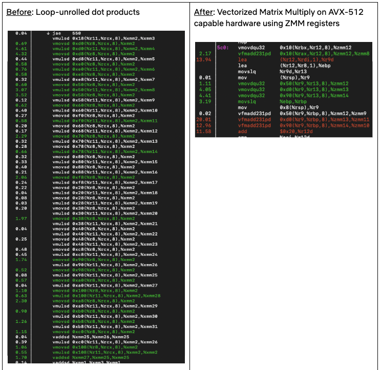
Assembly snippet from batchEncode

Closing Thoughts

This optimization ended up being less about finding the “fastest library” and more about getting the fundamentals right: choosing the right computation shape, keeping data layout cache-friendly, and avoiding overheads that can erase theoretical wins. Once those pieces were in place, the JDK Vector API was a great fit, as it let us express SIMD-style math in pure Java, without JNI, while still keeping a safe fallback path. Another bonus was the low developer overhead: compared to lower-level approaches, the Vector API let us replace a much larger, more complex implementation with a relatively small amount of readable Java code, which made it easier to review, maintain, and iterate on.

Have you tried the Vector API in a real service yet? I’d love to hear what workloads it helped (or didn’t), and what you learned about benchmarking and rollout in production.

Special thanks to Jason Koch, Patrick Strawderman, Daniel Huang, Fan Yang, and the Performance Engineering team at Netflix


Optimizing Recommendation Systems with JDK’s Vector API was originally published in Netflix TechBlog on Medium, where people are continuing the conversation by highlighting and responding to this story.


Building even faster interpreters in Rust

Post Syndicated from Zak Cutner original https://blog.cloudflare.com/building-even-faster-interpreters-in-rust/

Building even faster interpreters in Rust

Building even faster interpreters in Rust

At Cloudflare, we’re constantly working on improving the performance of our edge — and that was exactly what my internship this summer entailed. I’m excited to share some improvements we’ve made to our popular Firewall Rules product over the past few months.

Firewall Rules lets customers filter the traffic hitting their site. It’s built using our engine, Wirefilter, which takes powerful boolean expressions written by customers and matches incoming requests against them. Customers can then choose how to respond to traffic which matches these rules. We will discuss some in-depth optimizations we have recently made to Wirefilter, so you may wish to get familiar with how it works if you haven’t already.

Minimizing CPU usage

As a new member of the Firewall team, I quickly learned that performance is important — even in our security products. We look for opportunities to make our customers’ Internet properties faster where it’s safe to do so, maximizing both security and performance.

Our engine is already heavily used, powering all of Firewall Rules. But we have bigger plans. More and more products like our Web Application Firewall (WAF) will be running behind our Wirefilter-based engine, and it will become responsible for eating up a sizable chunk of our total CPU usage before long.

How to measure performance?

Measuring performance is a notoriously tricky task, and as you can probably imagine trying to do this in a highly distributed environment (aka Cloudflare’s edge) does not help. We’ve been surprised in the past by optimizations that look good on paper, but, when tested out in production, just don’t seem to do much.

Our solution? Performance measurement as a service — an isolated and reproducible benchmark for our Firewall engine and a framework for engineers to easily request runs and view results. It’s worth noting that we took a lot of inspiration from the fantastic Rust Compiler benchmarks to build this.

Building even faster interpreters in Rust
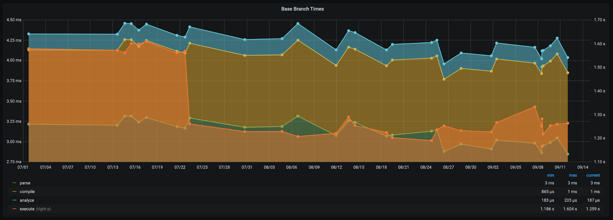
Our benchmarking framework, showing how performance during different stages of processing Wirefilter expressions has changed over time [1].

What to measure?

Our next challenge was to find some meaningful performance metrics. Some experimentation quickly uncovered that time was far too volatile a measure for meaningful comparisons, so we turned to hardware counters [2]. It’s not hard to find tools to measure these (perf and VTune are two such examples), although they (mostly) don’t allow control over which parts of the program are recorded. In our case, we wished to individually record measurements for different stages of filter processing — parsing, compilation, analysis, and execution.

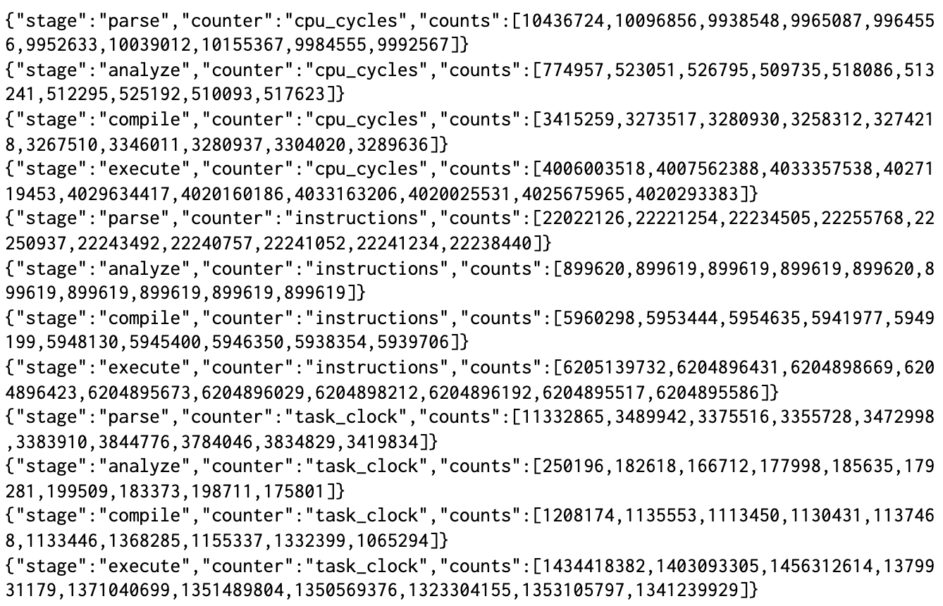
Once again we took inspiration from the Rust compiler, and its self-profiling options, using the perf_event_open API to record counters from inside our binary. We then output something like the following, which our framework can easily ingest and store for later visualization.

Building even faster interpreters in Rust
Output of our benchmarks in JSON Lines format, showing a list of recordings for each combination of hardware counter and Wirefilter processing stage. We’ve used 10 repeats here for readability, but we use around 20, in addition to 5 warmup rounds, within our framework.

Whilst we mainly focussed on metrics relating to CPU usage, we also use a combination of getrusage and clear_refs to find the maximum resident set size (RSS). This is useful to understand the memory impact of particular algorithms in addition to CPU.

But the challenge was not over. Cloudflare’s standard CI agents use virtualization and sandboxing for security and convenience, but this makes accessing hardware counters virtually impossible. Running our benchmarks on a dedicated machine gave us access to these counters, and ensured more reproducible results.

Speeding up the speed test

Our benchmarks were designed from the outset to take an important place in our development process. For instance, we now perform a full benchmark run before releasing each new version to detect performance regressions.

But with our benchmarks in place, it quickly became clear that we had a problem. Our benchmarks simply weren’t fast enough — at least if we wanted to complete them in less than a few hours! The problem was we have a very large number  of filters. Since our engine would never usually execute requests against this many filters at once it was proving incredibly costly. We came up with a few tricks to cut this down…

  • Deduplication. It turns out that only around a third of filters are structurally unique (something that is easy to check as Wirefilter can helpfully serialize to JSON). We managed to cut down a great deal of time by ignoring duplicate filters in our benchmarks.
  • Sampling. Still, we had too many filters and random sampling presented an easy solution. A more subtle challenge was to make sure that the random sample was always the same to maintain reproducibility.
  • Partitioning. We worried that deduplication and sampling would cause us to miss important cases that are useful to optimize. By first partitioning filters by Wirefilter language feature, we can ensure we’re getting a good range of filters. It also helpfully gives us more detail about where specifically the impact of a performance change is.

Most of these are trade-offs, but very necessary ones which allow us to run continual benchmarks without development speed grinding to a halt. At the time of writing, we’ve managed to get a benchmark run down to around 20 minutes using these ideas.

Optimizing our engine

With a benchmarking framework in place, we were ready to begin testing optimizations. But how do you optimize an interpreter like Wirefilter? Just-in-time (JIT) compilation, selective inlining and replication were some ideas floating around in the word of interpreters that seemed attractive. After all, we previously wrote about the cost of dynamic dispatch in Wirefilter. All of these techniques aim to reduce that effect.

However, running some real filters through a profiler tells a different story. Most execution time, around 65%, is spent not resolving dynamic dispatch calls but instead performing operations like comparison and searches. Filters currently in production tend to be pretty light on functions, but throw in a few more of these and even less time would be spent on dynamic dispatch. We suspect that even a fair chunk of the remaining 35% is actually spent reading the memory of request fields.

Function CPU time
`matches` operator 0.6%
`in` operator 1.1%
`eq` operator 11.8%
`contains` operator 51.5%
Everything else 35.0%
Breakdown of CPU time while executing a typical production filter.

An adventure in substring searching

By now, you shouldn’t be surprised that the contains operator was one of the first in line for optimization. If you’ve ever written a Firewall Rule, you’re probably already familiar with what it does — it checks whether a substring is present in the field you are matching against. For example, the following expression would match when the host is “example.com” or “www.example.net”, but not when it is “cloudflare.com”. In string searching algorithms, this is commonly referred to as finding a ‘needle’ (“example”) within a ‘haystack’ (“example.com”).

http.host contains “example”

How does this work under the hood? Ordinarily, we may have used Rust’s `String::contains` function but Wirefilter also allows raw byte expressions that don’t necessarily conform to UTF-8.

http.host contains 65:78:61:6d:70:6c:65

We therefore used the memmem crate which performs a two-way substring search algorithm on raw bytes.

Sounds good, right? It was, and it was working pretty well, although we’d noticed that rewriting `contains` filters using regular expressions could bizarrely often make them faster.

http.host matches “example”

Regular expressions are great, but since they’re far more powerful than the `contains` operator, they shouldn’t be faster than a specialized algorithm in simple cases like this one.

Something was definitely up. It turns out that Rust’s regex library comes equipped with a whole host of specialized matchers for what it deems to be simple expressions like this. The obvious question was whether we could therefore simply use the regex library. Interestingly, you may not have realized that the popular ripgrep tool does just that when searching for fixed-string patterns.

However, our use case is a little different. Since we’re building an interpreter (and we’re using dynamic dispatch in any case), we would prefer to dispatch to a specialized case for `contains` expressions, rather than matching on some enum deep within the regex crate when the filter is executed. What’s more, there are some pretty cool things being done to perform substring searching that leverages SIMD instruction sets. So we wired up our engine to some previous work by Wojciech Muła and the results were fantastic.

Benchmark Improvement
Expressions using `contains` operator 72.3%
‘Simple’ expressions 0.0%
All expressions 31.6%
Improvements in instruction count using Wojciech Muła’s sse4-strstr library over the memmem crate with Wirefilter.

I encourage you to read more on “Algorithm 1”, which we used, but it works something like this (I’ve changed the order a little to help make it clearer). It’s worth reading up on SIMD instructions if you’re unfamiliar with them — they’re the essence behind what makes this algorithm fast.

  1. We fill one SIMD register with the first byte of the needle being searched for, simply repeated over and over.
  2. We load as much of our haystack as we can into another SIMD register and perform a bitwise equality operation with our previous register.
  3. Now, any position in the resultant register that is 0 cannot be the start of the match since it doesn’t start with the same byte of the needle.
  4. We now repeat this process with the last byte of the needle, offsetting the haystack, to rule out any positions that don’t end with the same byte as the needle.
  5. Bitwise ANDing these two results together, we (hopefully) have now drastically reduced our potential matches.
  6. Each of the remaining potential matches can be checked manually using a memcmp operation. If we find a match, then we’re done.
  7. If not, we continue with the next part of our haystack and repeat until we’ve checked the entire thing.

When it goes wrong

You may be wondering what happens if our haystack doesn’t fit neatly into registers. In the original algorithm, nothing. It simply continues reading into the oblivion after the end of the haystack until the last register is full, and uses a bitmask to ignore potential false-positives from this additional region of memory.

As we mentioned, security is our priority when it comes to optimizations, so we could never deploy something with this kind of behaviour. We ended up porting Muła’s library to Rust (we’ve also open-sourced the crate!) and performed an overlapping registers modification found in ARM’s blog.

It’s best illustrated by example — notice the difference between how we would fill registers on an imaginary SIMD instruction-set with 4-byte registers.

Before modification

Building even faster interpreters in Rust
How registers are filled in the original implementation for the haystack “abcdefghij”, red squares indicate out of bounds memory.

After modification

Building even faster interpreters in Rust
How registers are filled with the overlapping modification for the same haystack, notice how ‘g’ and ‘h’ each appear in two registers.

In our case, repeating some bytes within two different registers will never change the final outcome, so this modification is allowed as-is. However, in reality, we found it was better to use a bitmask to exclude repeated parts of the final register and minimize the number of memcmp calls.

What if the haystack is too small to even fill a single register? In this case, we can’t use our overlapping trick since there’s nothing to overlap with. Our solution is straightforward: while we were primarily targeting AVX2, which can store 32-bytes in a lane, we can easily move down to another instruction set with smaller registers that the haystack can fit into. In reality, we don’t currently go any smaller than SSE2. Beyond this, we instead use an implementation of the Rabin-Karp searching algorithm which appears to perform well.

Instruction set Register size
AVX2 32 bytes
SSE2 16 bytes
SWAR (u64) 8 bytes
SWAR (u32) 4 bytes
Register sizes in different SIMD instruction sets [3]. We did not consider AVX512 since support for this is not widespread enough.

Is it always fast?

Choosing the first and last bytes of the needle to rule out potential matches is a great idea. It means that when it does come to performing a memcmp, we can ignore these, as we know they already match. Unfortunately, as Muła points out, this also makes the algorithm susceptible to a worst-case attack in some instances.

Let’s give an expression that a customer might write to illustrate this.

http.request.uri.path contains “/wp-admin/”

If we try to search for this within a very long sequence of ‘/’s, we will find a potential match in every position and make lots of calls to memcmp — essentially performing a slow bruteforce substring search.

Clearly we need to choose different bytes from the needle. But which ones should we choose? For each choice, an adversary can always find a slightly different, but equally troublesome, worst case. We instead use randomness to throw off our would-be adversary, picking the first byte of the needle as before, but then choosing another random byte to use.

Our new version is unsurprisingly slower than Muła’s, yet it still exhibits a great improvement over both the memmem and regex crates. Performance, but without sacrificing safety.

Benchmark Improvement
sse4-strstr (original) sliceslice (our version)
Expressions using `contains` operator 72.3% 49.1%
‘Simple’ expressions 0.0% 0.1%
All expressions 31.6% 24.0%
Improvements in instruction count of using sse4-strstr and sliceslice over the memmem crate with Wirefilter.

What’s next?

This is only a small taste of the performance work we’ve been doing, and we have much more yet to come. Nevertheless, none of this would have been possible without the support of my manager Richard and my mentor Elie, who contributed a lot of these ideas. I’ve learned so much over the past few months, but most of all that Cloudflare is an amazing place to be an intern!

[1] Since our benchmarks are not run within a production environment, results in this post do not represent traffic on our edge.

[2] We found instruction counts to be a particularly stable measure, and CPU cycles a particularly unstable one.

[3] Note that SWAR is technically not an instruction set, but instead uses regular registers like vector registers.