Post Syndicated from Harsha Tadiparthi original https://aws.amazon.com/blogs/big-data/scale-read-and-write-workloads-with-amazon-redshift/
Amazon Redshift is a fast, fully managed, petabyte-scale cloud data warehouse that enables you to analyze large datasets using standard SQL. The concurrency scaling feature in Amazon Redshift automatically adds and removes capacity by adding concurrency scaling to handle demands from thousands of concurrent users, thereby providing consistent SLAs for unpredictable and spiky workloads such as BI reports, dashboards, and other analytics workloads.
Until now, concurrency scaling only supported auto scaling for read queries; write queries had to run on the main cluster. Now, we are extending concurrency scaling to support auto scaling for common write queries including COPY, INSERT, UPDATE, and DELETE. This is available on Amazon Redshift RA3 provisioned instance types in the Regions where concurrency scaling is available. Amazon Redshift serverless comes with built in dynamic auto scaling capability for read workload scaling.
In this post, we discuss how to enable concurrency scaling to offer consistent SLAs for concurrent workloads such as data loads, ETL (extract, transform, and load), and data processing with reduced queue times.
Concurrency scaling overview
With concurrency scaling, Amazon Redshift automatically and elastically scales query processing power to provide consistently fast performance for hundreds of concurrent queries. Concurrency scaling resources are added to your Amazon Redshift cluster transparently in seconds, as concurrency increases, to serve sudden spikes in concurrent requests with fast performance without wait time. When the workload demand subsides, Amazon Redshift automatically shuts down concurrency scaling resources to save you cost.
The following diagram shows how concurrency scaling works at a high level.
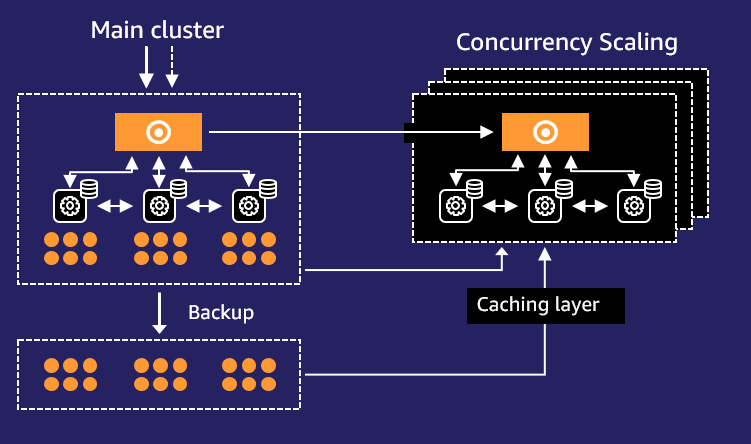
The workflow contains the following steps:
- All queries go to the main cluster.
- When queries in the designated workload management (WLM) queue begin queuing, Amazon Redshift automatically routes eligible queries to the new clusters, enabling concurrency scaling.
- Amazon Redshift automatically spins up a new cluster, processes waiting queries, and shuts down the concurrency scaling cluster when no longer needed.
Enable Amazon Redshift concurrency scaling
You can manage concurrency scaling at the WLM queue level, where you set concurrency scaling policies for specific queues. When concurrency scaling is enabled for a queue, eligible write and read queries are sent to concurrency scaling clusters without having to wait for resources to free up on the main Amazon Redshift cluster. Amazon Redshift handles spinning up concurrency scaling clusters, routing of the queries to the transient clusters, and relinquishing the concurrency clusters.
You can enable concurrency scaling on both automatic and manual WLM.
You first need to determine which parameter group your cluster is. To do so, complete the following steps:
- On the Amazon Redshift console, choose Clusters in the navigation pane.
- Choose your cluster.

- On the Properties tab, note the parameter group associated to the cluster.
 Now you can configure your WLM parameters.
 - Under Configurations in the navigation pane, choose Workload management.
- Choose the parameter group associated to the cluster.If you’re using the default parameter group default.redshift-1.0, you need to create a custom parameter group and assign that to the cluster. The default parameter group has preset values for each of its parameters, and it can’t be modified.
- On the Parameters tab, you can choose between 1–10
max_concurrency_scaling_clusters.This is the max number of concurrent Amazon Redshift clusters you can have running at the same time. Ten is the soft limit; this limit can be increased by submitting a service limit increase request with a support case.
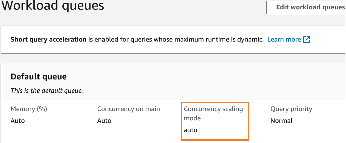
- On the Workload management tab, choose auto mode for the concurrency scaling cluster.


Example use cases
In this section, we use three use cases to help you understand how concurrency scaling for read and write heavy workloads can seamlessly scale to improve workload performance SLAs.
We used a 3 TB Cloud DW benchmark dataset. The test included a total of 103 concurrent queries, with each run using a separate database connection. The 103 queries constituted 60 queries from the 99 TPC-DS queries and 43 write queries, with a mix of copy, insert, update and delete statements. We used RA3.4xlarge 5 compute nodes.
The following scenarios showcase how concurrency scaling for reads and writes can seamlessly auto scale and positively impact a heavy concurrent mixed workload:
- All queries triggered concurrently with concurrency scaling turned off
- All queries triggered concurrently with concurrency scaling cluster limit set to 5 clusters
- All queries triggered concurrently with concurrency scaling cluster limit set to 10 clusters
Scenario 1: All queries triggered concurrently with concurrency scaling turned off
In this benchmark test, all queries completed in 299 minutes. The following are the test details.
The Amazon Redshift query optimizer turned the 103 queries into 257 sub-queries for better performance in this run. Amazon Redshift continuous to learn from operational statistics to optimize your workload.
The following screenshot shows how Amazon Redshift auto WLM mode chose to run 16 queries concurrently while queuing the rest. Because concurrency scaling is turned off, no additional clusters are spun up and the queries continue to wait for running queries to complete before they can be processed. Notice the number of queries queued stayed at a higher number for a long period of time and eventually lowered as only a few queries could concurrently run.

No additional concurrent clusters spun up during the window of the workload, as seen in the following screenshot, requiring the primary cluster to process all the queries.

Scenario 2: All queries triggered concurrently with concurrency scaling cluster max limit set to 5 clusters
In this test, all queries completed in 49 minutes.
The following screenshot depicts significant queuing. Within seconds, five additional Amazon Redshift clusters are spun up into ready state, allowing 53 queries to run simultaneously. This number can change in your cluster based on the query types. Notice the number of queries queued starts lowering as more queries are completed using the five additional clusters.
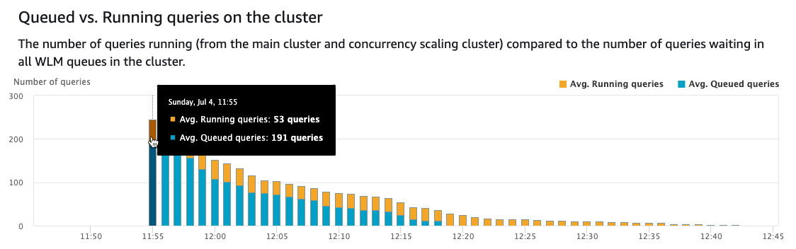
Over time, the concurrency scaling clusters start to wind down progressively to 0 as the queries no longer waited.

Scenario 3: All queries triggered concurrently with concurrency scaling cluster limit set to 10 clusters
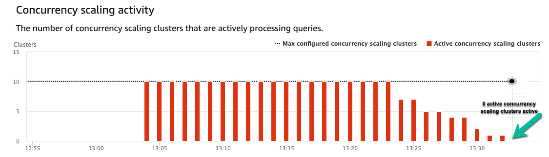
In this test, all queries completed in 28 minutes.
The following screenshot depicts significant queuing. Within seconds, 10 additional Amazon Redshift clusters are spun up into ready state, allowing multiple queries to run simultaneously. This number can change in your cluster based on the query types. Notice the number of queries queued starts lowering as more queries are completed using the five additional clusters.

Over time, the concurrency scaling clusters start to wind down progressively to 0 as the queries no longer waited.
Test results review
The following table summarizes our test results.
| . | Test Scenario 1 | Test Scenario 2 | Test Scenario 3 |
| Total Workload Completion Time | 299 Minutes | 49 Minutes | 28 Minutes |
The test results reveal how concurrency scaling for a mixed workload of reads and writes lowered the total workload completion time from 299 minutes to 28 minutes, which is more than 10 times an improvement in SLAs while being cost effective by only paying for the additional clusters when scaling is necessary.
Monitor concurrency scaling
One method to monitor concurrency scaling is via system views. To monitor which queries benefitted from concurrency scaling, you can use concurrency_scaling_status from stl_query. Concurrency scaling of 1 indicates that the query ran on a concurrency scaling cluster. To monitor concurrency scaling usage, you can use the SVCS_CONCURRENCY_SCALING_USAGE system view.
The Amazon CloudWatch metrics ConcurrencyScalingActiveClusters and ConcurrencyScalingSeconds enable you to set up monitoring of concurrency scaling usage. For more information, refer to Monitoring Amazon Redshift using CloudWatch metrics.
Configure usage limit
With every 24 hours used of the main Amazon Redshift cluster, you accrue 1 hour of concurrency scaling credit. This free credit can be used by both read and write queries. For any usage that exceeds the accrued free usage credits, you’re billed on a per-second basis based on the on-demand rate of your Amazon Redshift cluster. You can apply cost controls for concurrency scaling at the cluster level. You can choose to create multiple queues for ETL, Dashboard, and adhoc workload. With this you can choose to turn on concurrency scaling for selective queues.
As shown in the following screenshot, you can choose a time period (daily, weekly, or monthly) and specify the desired usage limit. You can then choose an action option (Alert, Log to system table, or Disable feature). For more details on how to set cost controls for concurrency scaling, refer to Manage and control your cost with Amazon Redshift Concurrency Scaling and Spectrum.

Summary
In this post, we showed how you can enable concurrency scaling to help you meet the SLAs for both read and write workloads by seamlessly scaling out to the maximum number of clusters you configured, thereby increasing your cluster throughput while controlling your costs. Concurrency scaling with read and write capability can enable you to handle a number of scenarios, such as sudden increases in the volume of data in your data pipeline, backfill operations, ad hoc reporting, and month end processing. It’s now time to put this learning into action and begin optimizing your Redshift cluster(s) for both read and write throughput!
About the Authors
 Harsha Tadiparthi is a specialist Principal Solutions Architect, Analytics at AWS. He enjoys solving complex customer problems in databases and analytics and delivering successful outcomes. Outside of work, he loves to spend time with his family, watch movies, and travel whenever possible.
 Harshida Patel is a Specialist Principal Solutions Architect, Analytics with AWS.
 Ramu Ponugumati is a Sr. Technical Account Manager, specialist in Analytics and AI/ML at AWS. He works with enterprise customers to modernize and cost optimize workloads, and helps them build reliable and secure applications on the AWS platform. Outside of work, he loves spending time with his family, playing tennis, and gardening.


 Harsha Tadiparthi is a Specialist Sr. Solutions Architect, AWS Analytics. He enjoys solving complex customer problems in Databases and Analytics and delivering successful outcomes. Outside of work, he loves to spend time with his family, watch movies, and travel whenever possible.
 Harshida Patel is a Specialist Sr. Solutions Architect, Analytics with AWS.


 Harsha Tadiparthi is a Specialist Sr. Solutions Architect, AWS Analytics. He enjoys solving complex customer problems in Databases and Analytics and delivering successful outcomes. Outside of work, he loves to spend time with his family, watch movies, and travel whenever possible.