Tag Archives: Data Lake

Modernize your legacy databases with AWS data lakes, Part 2: Build a data lake using AWS DMS data on Apache Iceberg

2024-10-30 Shaheer Mansoor

Post Syndicated from Shaheer Mansoor original https://aws.amazon.com/blogs/big-data/modernize-your-legacy-databases-with-aws-data-lakes-part-2-build-a-data-lake-using-aws-dms-data-on-apache-iceberg/

This is part two of a three-part series where we show how to build a data lake on AWS using a modern data architecture. This post shows how to load data from a legacy database (SQL Server) into a transactional data lake (Apache Iceberg) using AWS Glue. We show how to build data pipelines using AWS Glue jobs, optimize them for both cost and performance, and implement schema evolution to automate manual tasks. To review the first part of the series, where we load SQL Server data into Amazon Simple Storage Service (Amazon S3) using AWS Database Migration Service (AWS DMS), see Modernize your legacy databases with AWS data lakes, Part 1: Migrate SQL Server using AWS DMS.

Solution overview

In this post, we go over the process of building a data lake, providing the rationale behind the different decisions, and share best practices when building such a solution.

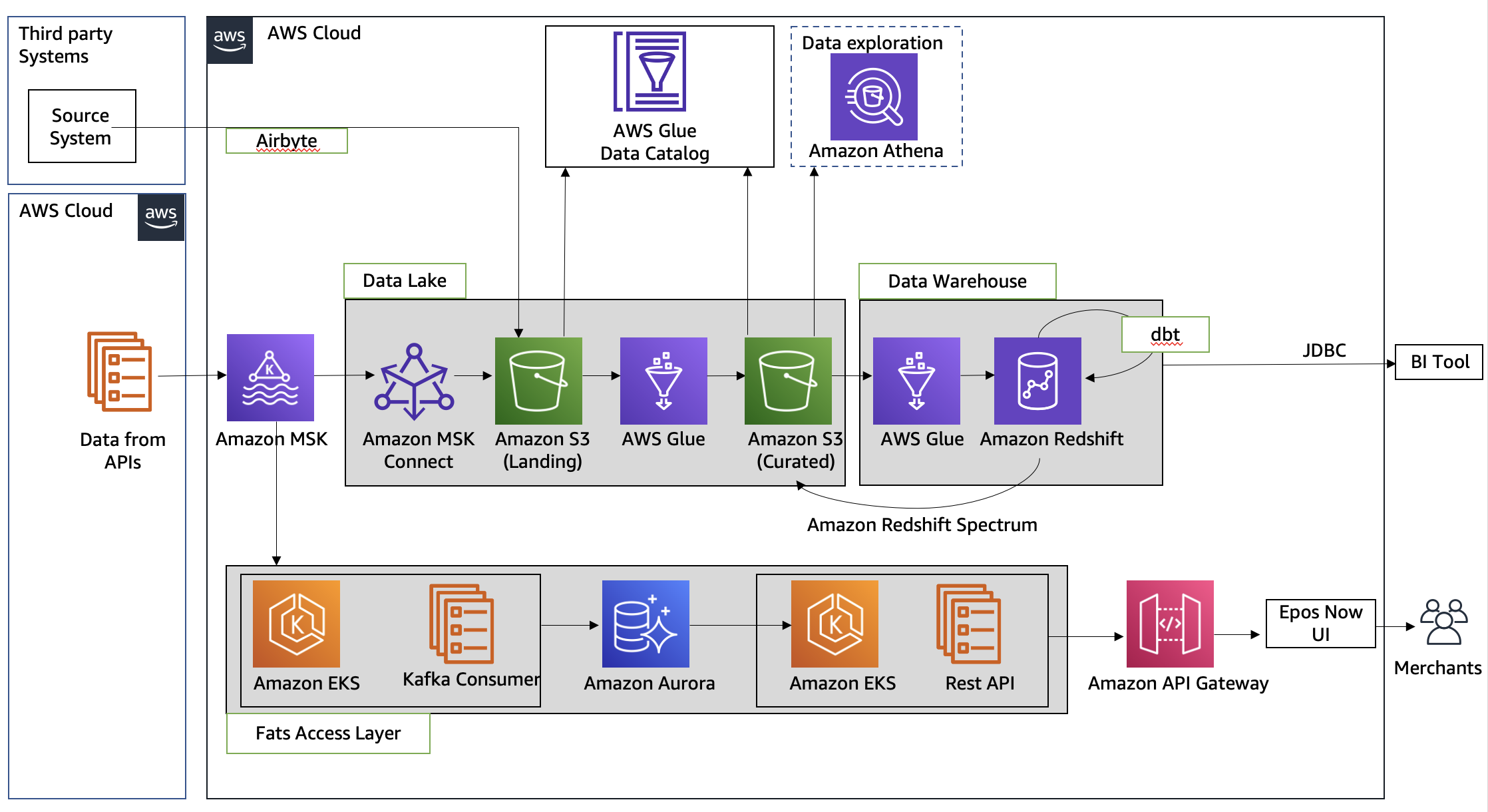
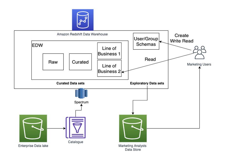
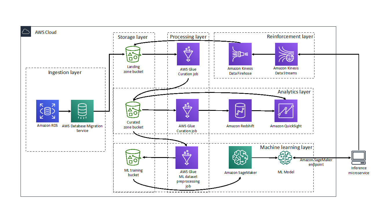
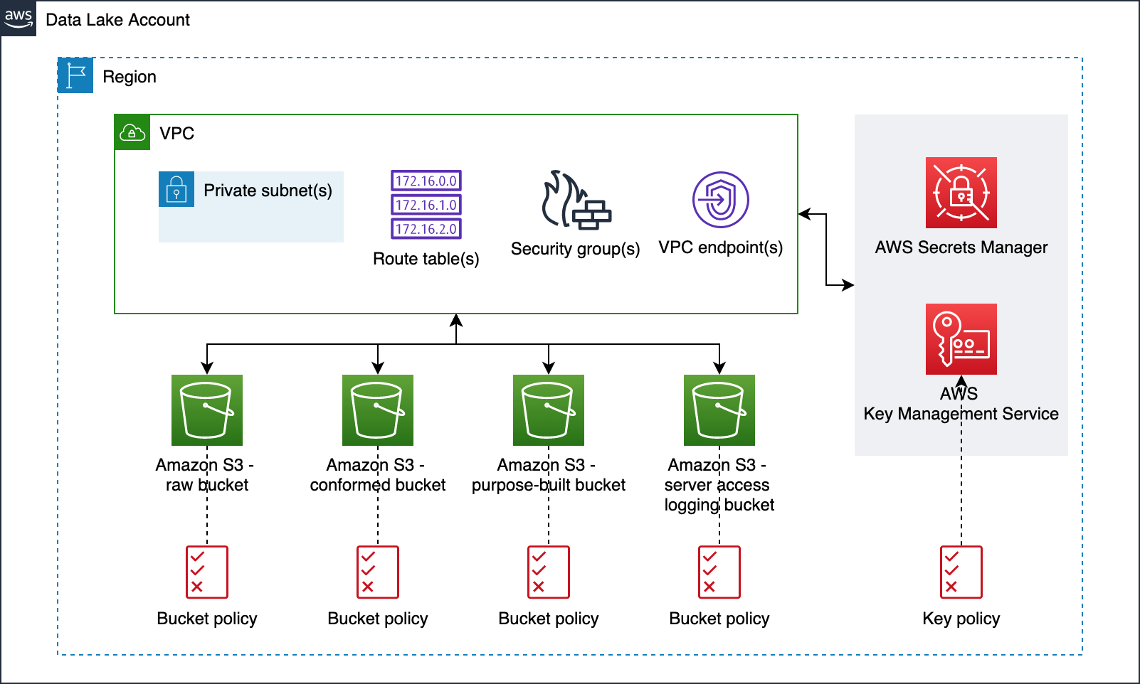
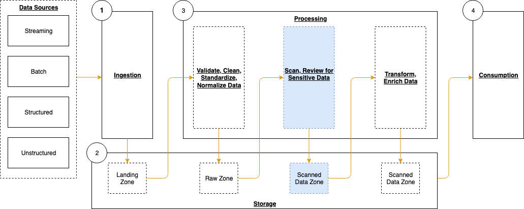
The following diagram illustrates the different layers of the data lake.

Overall Architecture

To load data into the data lake, AWS Step Functions can define a workflow, Amazon Simple Queue Service (Amazon SQS) can track the order of incoming files, and AWS Glue jobs and the Data Catalog can be used create the data lake silver layer. AWS DMS produces files and writes these files to the bronze bucket (as we explained in Part 1).

We can turn on Amazon S3 notifications and push the new arriving file names to an SQS first-in-first-out (FIFO) queue. A Step Functions state machine can consume messages from this queue to process the files in the order they arrive.

For processing the files, we need to create two types of AWS Glue jobs:

Full load – This job loads the entire table data dump into an Iceberg table. Data types from the source are mapped to an Iceberg data type. After the data is loaded, the job updates the Data Catalog with the table schemas.
CDC – This job loads the change data capture (CDC) files into the respective Iceberg tables. The AWS Glue job implements the schema evolution feature of Iceberg to handle schema changes such as addition or deletion of columns.

As in Part 1, the AWS DMS jobs will place the full load and CDC data from the source database (SQL Server) in the raw S3 bucket. Now we process this data using AWS Glue and save it to the silver bucket in Iceberg format. AWS Glue has a plugin for Iceberg; for details, see Using the Iceberg framework in AWS Glue.

Along with moving data from the bronze to the silver bucket, we also create and update the Data Catalog for further processing the data for the gold bucket.

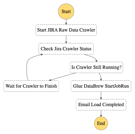
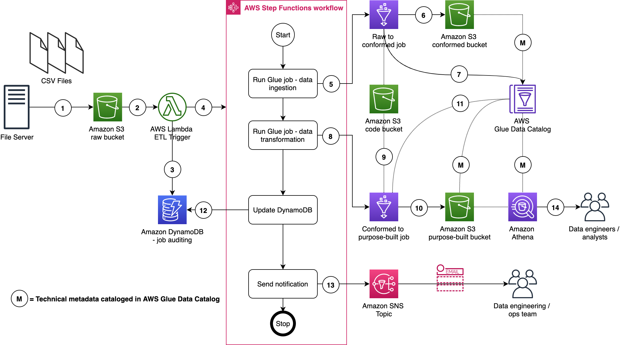
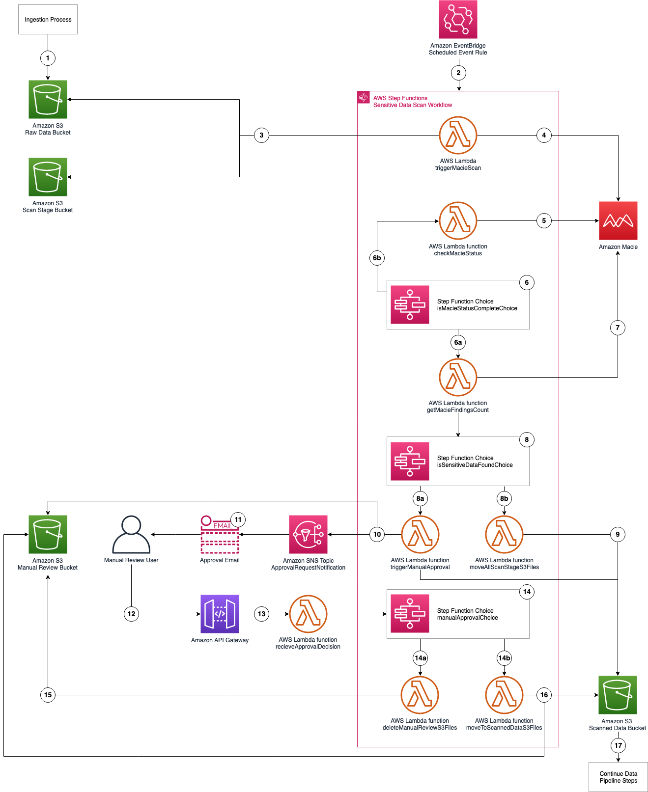
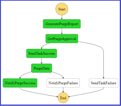
The following diagram illustrates how the full load and CDC jobs are defined inside the Step Functions workflow.

Step Functions for loading data into the lake

In this post, we discuss the AWS Glue jobs for defining the workflow. We recommend using AWS Step Functions Workflow Studio, and setting up Amazon S3 event notifications and an SNS FIFO queue to receive the filename as messages.

Prerequisites

To follow the solution, you need the following prerequisites set up as well as certain access rights and AWS Identity and Access Management (IAM) privileges:

An IAM role to run Glue jobs
IAM privileges to create AWS DMS resources (this role was created in Part 1 of this series; you can use the same role here)
The AWS DMS job from Part 1 working and producing files for the source database on Amazon S3.

Create an AWS Glue connection for the source database

We need to create a connection between AWS Glue and the source SQL Server database so the AWS Glue job can query the source for the latest schema while loading the data files. To create the connection, follow these steps:

On the AWS Glue console, choose Connections in the navigation pane.
Choose Create custom connector.
Give the connection a name and choose JDBC as the connection type.
In the JDBC URL section, enter the following string and replace the name of your source database endpoint and database that was set up in Part 1: jdbc:sqlserver://{Your RDS End Point Name}:1433/{Your Database Name}.
Select Require SSL connection, then choose Create connector.

Clue Connections

Create and configure the full load AWS Glue job

Complete the following steps to create the full load job:

On the AWS Glue console, choose ETL jobs in the navigation pane.
Choose Script editor and select Spark.
Choose Start fresh and select Create script.
Enter a name for the full load job and choose the IAM role (mentioned in the prerequisites) for running the job.
Finish creating the job.
On the Job details tab, expand Advanced properties.
In the Connections section, add the connection you created.
Under Job parameters, pass the following arguments to the job:
1. target_s3_bucket – The silver S3 bucket name.
2. source_s3_bucket – The raw S3 bucket name.
3. secret_id – The ID of the AWS Secrets Manager secret for the source database credentials.
4. dbname – The source database name.
5. datalake-formats – This sets the data format to iceberg.

Glue Job Parameters

The full load AWS Glue job starts after the AWS DMS task reaches 100%. The job loops over the files located in the raw S3 bucket and processes them one at time. For each file, the job infers the table name from the file name and gets the source table schema, including column names and primary keys.

If the table has one or more primary keys, the job creates an equivalent Iceberg table. If the job has no primary key, the file is not processed. In our use case, all the tables have primary keys, so we enforce this check. Depending on your data, you might need to handle this scenario differently.

You can use the following code to process the full load files. To start the job, choose Run.

import sys, boto3, json
import boto3
import json
from awsglue.utils import getResolvedOptions
from pyspark.context import SparkContext
from awsglue.context import GlueContext
from awsglue.job import Job
from pyspark.sql import SparkSession

#Get the arguments passed to the script
args = getResolvedOptions(sys.argv, ['JOB_NAME',
                           'target_s3_bucket',
                           'secret_id',
                           'source_s3_bucket'])
dbname = "AdventureWorks"
schema = "HumanResources"

#Initialize parameters
target_s3_bucket = args['target_s3_bucket']
source_s3_bucket = args['source_s3_bucket']
secret_id = args['secret_id']
unprocessed_tables = []
drop_column_list = ['db', 'table_name', 'schema_name', 'Op', 'last_update_time']  # DMS added columns

#Helper Function: Get Credentials from Secrets Manager
def get_db_credentials(secret_id):
    secretsmanager = boto3.client('secretsmanager')
    response = secretsmanager.get_secret_value(SecretId=secret_id)
    secrets = json.loads(response['SecretString'])
    return secrets['host'], int(secrets['port']), secrets['username'], secrets['password']

#Helper Function: Load Iceberg table with Primary key(s)
def load_table(full_load_data_df, dbname, table_name):

    try:
        full_load_data_df = full_load_data_df.drop(*drop_column_list)
        full_load_data_df.createOrReplaceTempView('full_data')

        query = """
        CREATE TABLE IF NOT EXISTS glue_catalog.{0}.{1}
        USING iceberg
        LOCATION "s3://{2}/{0}/{1}"
        AS SELECT * FROM full_data
        """.format(dbname, table_name, target_s3_bucket)
        spark.sql(query)
        
        #Update Table property to accept Schema Changes
        spark.sql("""ALTER TABLE glue_catalog.{0}.{1} SET TBLPROPERTIES (
                      'write.spark.accept-any-schema'='true'
                    )""".format(dbname, table_name))
        
    except Exception as ex:
        print(ex)
        failed_table = {"table_name": table_name, "Reason": ex}
        unprocessed_tables.append(failed_table)
        
def get_table_key(host, port, username, password, dbname):
    
    jdbc_url = "jdbc:sqlserver://{0}:{1};databaseName={2}".format(host, port, dbname)
    
    connectionProperties = {
      "user" : username,
      "password" : password
    }
    
    spark.read.jdbc(url=jdbc_url, table='INFORMATION_SCHEMA.TABLE_CONSTRAINTS', properties=connectionProperties).createOrReplaceTempView("TABLE_CONSTRAINTS")
    spark.read.jdbc(url=jdbc_url, table='INFORMATION_SCHEMA.CONSTRAINT_COLUMN_USAGE', properties=connectionProperties).createOrReplaceTempView("CONSTRAINT_COLUMN_USAGE")
    df_table_pkeys = spark.sql("select c.TABLE_NAME, C.COLUMN_NAME as primary_key FROM TABLE_CONSTRAINTS T JOIN CONSTRAINT_COLUMN_USAGE C ON C.CONSTRAINT_NAME=T.CONSTRAINT_NAME WHERE T.CONSTRAINT_TYPE='PRIMARY KEY'")
    return df_table_pkeys


#Setup Spark configuration for reading and writing Iceberg tables
spark = (
    SparkSession.builder
    .config("spark.sql.extensions", "org.apache.iceberg.spark.extensions.IcebergSparkSessionExtensions")
    .config("spark.sql.catalog.glue_catalog", "org.apache.iceberg.spark.SparkCatalog")
    .config("spark.sql.catalog.glue_catalog.warehouse", "s3://{0}".format(dbname))
    .config("spark.sql.catalog.glue_catalog.catalog-impl", "org.apache.iceberg.aws.glue.GlueCatalog")
    .config("spark.sql.catalog.glue_catalog.io-impl", "org.apache.iceberg.aws.s3.S3FileIO")
    .getOrCreate()
)


#Initialize MSSQL credentials
host, port, username, password = get_db_credentials(secret_id)

#Initialize primary keys for all tables
df_table_pkeys = get_table_key(host, port, username, password, dbname)

#Read Full load csv files from s3
s3 = boto3.client('s3')
full_load_tables = s3.list_objects_v2(Bucket=source_s3_bucket, Prefix="raw/{0}/{1}".format(args['dbname'], args['schema']))

#Loop over files
for item in full_load_tables['Contents']:
    pkey_list = []
    table_name = item["Key"].split("/")[3].lower()
    print("Table name {0}".format(table_name))
    current_table_df = df_table_pkeys.where(df_table_pkeys.TABLE_NAME == table_name)

    # Only Process tables with at least 1 Primary key
    if not current_table_df.isEmpty():
        for i in current_table_df.collect():
            pkey_list.append(i["primary_key"])
    else:
        failed_table = {"table_name": table_name, "Reason": "No primary key"}
        unprocessed_tables.append(failed_table)
        # ToDo Handle these cases

    full_data_path = "s3://{0}/{1}".format(source_s3_bucket, item['Key'])
    full_load_data_df = (spark
                        .read
                        .option("header", True)
                        .option("inferSchema", True)
                        .option("recursiveFileLookup", "true")
                        .csv(full_data_path)
                        )

    primary_key = ",".join(pkey_list)

    if table_name not in unprocessed_tables:
        load_table(full_load_data_df, dbname, table_name)

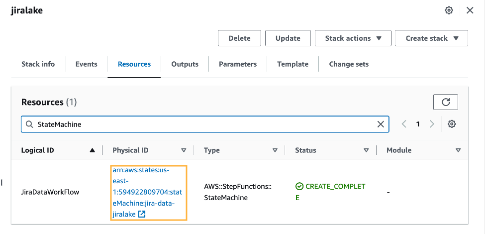
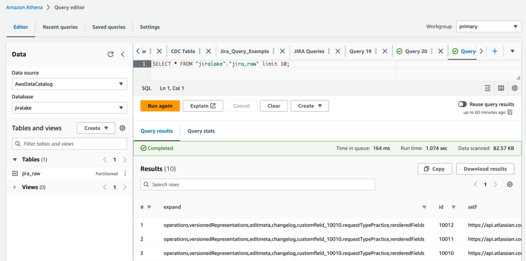
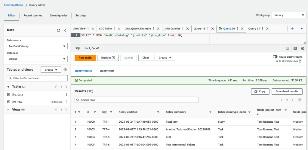
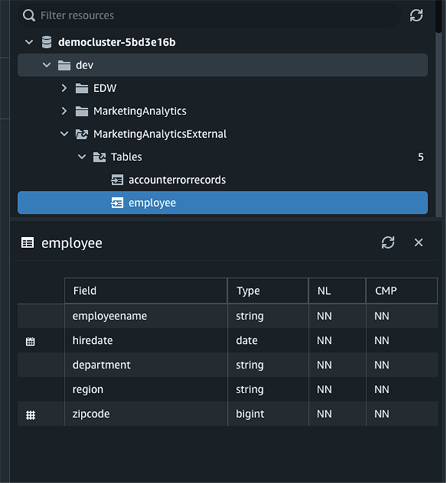
When the job is complete, it creates the database and tables in the Data Catalog, as shown in the following screenshot.

Data lake silver layer data

Create and configure the CDC AWS Glue job

The CDC AWS Glue job is created similar to the full load job. As with the full load AWS Glue job, you need to use the source database connection and pass the job parameters with one additional parameter, cdc_file, which contains the location of the CDC file to be processed. Because a CDC file can contain data for multiple tables, the job loops over the tables in a file and loads the table metadata from the source table ( RDS column names).

If the CDC operation is DELETE, the job deletes the records from the Iceberg table. If the CDC operation is INSERT or UPDATE, the job merges the data into the Iceberg table.

You can use the following code to process the CDC files. To start the job, choose Run

import sys
import boto3
import json
from awsglue.utils import getResolvedOptions
from pyspark.context import SparkContext
from awsglue.context import GlueContext
from awsglue.job import Job
from pyspark.sql import SparkSession

# Get the arguments passed to the script
args = getResolvedOptions(sys.argv, ['JOB_NAME',
                           'target_s3_bucket',
                           'secret_id',
                           'source_s3_bucket',
                           'cdc_file'])
dbname = "AdventureWorks"
schema = "HumanResources"
target_s3_bucket = args['target_s3_bucket']
source_s3_bucket = args['source_s3_bucket']
secret_id = args['secret_id']
cdc_file = args['cdc_file']
unprocessed_tables = []
drop_column_list = ['db', 'table_name', 'schema_name', 'Op', 'last_update_time']  # DMS added columns
source_s3_cdc_file_key = "raw/AdventureWorks/cdc/" + cdc_file



# Helper Function: Get Credentials from Secrets Manager
def get_db_credentials(secret_id):
    secretsmanager = boto3.client('secretsmanager')
    response = secretsmanager.get_secret_value(SecretId=secret_id)
    secrets = json.loads(response['SecretString'])
    return secrets['host'], int(secrets['port']), secrets['username'], secrets['password']

# Helper Function: Column names from RDS
def get_table_colums(table, host, port, username, password, dbname):

    jdbc_url = "jdbc:sqlserver://{0}:{1};databaseName={2}".format(host, port, dbname)
    
    connectionProperties = {
      "user" : username,
      "password" : password
    }
    
    spark.read.jdbc(url=jdbc_url, table='INFORMATION_SCHEMA.COLUMNS', properties= connectionProperties).createOrReplaceTempView("TABLE_COLUMNS")
    columns = list((row.COLUMN_NAME) for (index, row) in spark.sql("select TABLE_NAME, TABLE_CATALOG, COLUMN_NAME from TABLE_COLUMNS where TABLE_NAME = '{0}' and TABLE_CATALOG = '{1}'".format(table, dbname)).select("COLUMN_NAME").toPandas().iterrows())
    return columns

# Helper Function: Get Colum names and datatypes from RDS
def get_table_colum_datatypes(table, host, port, username, password, dbname):

    jdbc_url = "jdbc:sqlserver://{0}:{1};databaseName={2}".format(host, port, dbname)
    
    connectionProperties = {
      "user" : username,
      "password" : password
    }
    
    spark.read.jdbc(url=jdbc_url, table='INFORMATION_SCHEMA.COLUMNS', properties= connectionProperties).createOrReplaceTempView("TABLE_COLUMNS")
    return spark.sql("select TABLE_NAME, COLUMN_NAME, DATA_TYPE from TABLE_COLUMNS WHERE TABLE_NAME ='{0}'".format(table))

# Helper Function: Setup the primary key condition
def get_iceberg_table_condition(database, tablename):
    
    jdbc_url = "jdbc:sqlserver://{0}:{1};databaseName={2}".format(host, port, database)
    
    connectionProperties = {
      "user" : username,
      "password" : password
    }
    
    spark.read.jdbc(url=jdbc_url, table='INFORMATION_SCHEMA.TABLE_CONSTRAINTS', properties=connectionProperties).createOrReplaceTempView("TABLE_CONSTRAINTS")
    spark.read.jdbc(url=jdbc_url, table='INFORMATION_SCHEMA.CONSTRAINT_COLUMN_USAGE', properties=connectionProperties).createOrReplaceTempView("CONSTRAINT_COLUMN_USAGE")
    
    condition = ''
    
    for key in spark.sql("select C.COLUMN_NAME FROM TABLE_CONSTRAINTS T JOIN CONSTRAINT_COLUMN_USAGE C ON C.CONSTRAINT_NAME=T.CONSTRAINT_NAME WHERE T.CONSTRAINT_TYPE='PRIMARY KEY' AND c.TABLE_NAME = '{0}'".format(table)).collect():
        condition += "target.{0} = source.{0} and".format(key.COLUMN_NAME)
    return condition[:-4]

    
# Read incoming data from Amazon S3
def read_cdc_S3(source_s3_bucket, source_s3_cdc_file_key):
    
    inputDf = (spark
                    .read
                    .option("header", False)
                    .option("inferSchema", True)
                    .option("recursiveFileLookup", "true")
                    .csv("s3://" + source_s3_bucket + "/" + source_s3_cdc_file_key)
                    )
    return inputDf

# Setup Spark configuration for reading and writing Iceberg tables
spark = (
    SparkSession.builder
    .config("spark.sql.extensions", "org.apache.iceberg.spark.extensions.IcebergSparkSessionExtensions")
    .config("spark.sql.catalog.glue_catalog", "org.apache.iceberg.spark.SparkCatalog")
    .config("spark.sql.catalog.glue_catalog.warehouse", "s3://{0}".format(target_s3_bucket))
    .config("spark.sql.catalog.glue_catalog.catalog-impl", "org.apache.iceberg.aws.glue.GlueCatalog")
    .config("spark.sql.catalog.glue_catalog.io-impl", "org.apache.iceberg.aws.s3.S3FileIO")
    .getOrCreate()
)

#Initialize MSSQL credentials
host, port, username, password = get_db_credentials(secret_id)

#Read the cdc file 
cdc_df = read_cdc_S3(source_s3_bucket, source_s3_cdc_file_key)

tables = cdc_df.toPandas()._c1.unique().tolist()

#Loop over tables in the cdc file
for table in tables:
    #Create dataframes for delets and for inserts and updates
    table_df_deletes = cdc_df.where((cdc_df._c1 == table) & (cdc_df._c0 == "D")).drop(cdc_df.columns[0], cdc_df.columns[1], cdc_df.columns[2], cdc_df.columns[3])
    table_df_upserts = cdc_df.where((cdc_df._c1 == table) & ((cdc_df._c0 == "I") | (cdc_df._c0 == "U"))).drop(cdc_df.columns[0], cdc_df.columns[1], cdc_df.columns[2], cdc_df.columns[3])
    
    #Update column names for the dataframes
    columns = get_table_colums(table, host, port, username, password, dbname) 
    selectExpr = [] 

    for column in columns: 
        selectExpr.append(cdc_df.where((cdc_df._c1 == table)).drop(cdc_df.columns[0], cdc_df.columns[1], cdc_df.columns[2], cdc_df.columns[3]).columns[columns.index(column)] + " as " + column)

    table_df_deletes = table_df_deletes.selectExpr(selectExpr) 
    table_df_upserts = table_df_upserts.selectExpr(selectExpr)
    
    #Process Deletes
    if table_df_deletes.count() > 0:
        
        print("Delete Triggered")
        table_df_deletes.createOrReplaceTempView('deleted_rows')
        
        sql_string = """MERGE INTO glue_catalog.{0}.{1} target
                        USING (SELECT * FROM deleted_rows) source
                        ON {2}
                        WHEN MATCHED 
                        THEN DELETE""".format(database, table.lower(), get_iceberg_table_condition(database, table.lower()))
        spark.sql(sql_string)
    
    if table_df_upserts.count() > 0:
        print("Upsert triggered")

        #Upsert Records when there are Schema Changes
        if len(table_df_upserts.columns) != len(columns):

            #Handle column deletes
            if len(table_df_upserts.columns) < len(columns):

                drop_columns = list(set(columns) - set(table_df_upserts.columns))

                for drop_column in drop_columns:
                    sql_string = """
                                    ALTER TABLE glue_catalog.{0}.{1}
                                    DROP COLUMN {2}""".format(dbname.lower(), table.lower(), drop_column)
                    spark.sql(sql_string)

            #Handle column additions
            elif len(table_df_upserts.columns) > len(columns):

                column_datatype_df = get_table_colum_datatypes(table, host, port, username, password, dbname)
                add_columns = list(set(table_df_upserts.columns) - set(columns))

                for add_column in add_columns:

                    #Set Iceberg data type
                    data_type = list((row.DATA_TYPE) for (index, row) in column_datatype_df.filter("COLUMN_NAME='{0}'".format(add_column)).select("DATA_TYPE").toPandas().iterrows())[0]

                    # Convert MSSQL Datatypes to Iceberg supported datatypes
                    if data_type.lower() in ["varchar", "char"]:
                        data_type = "string"

                    if data_type.lower() in ["bigint"]:
                        data_type = "long"

                    if data_type.lower() in ["array"]:
                        data_type = "list"

                    sql_string = """
                                    ALTER TABLE glue_catalog.{0}.{1}
                                    ADD COLUMN {2} {3}""".format(dbname.lower(), table.lower(), add_column, data_type)
                    spark.sql(sql_string)
                    
            #Create statement to update columns
            update_table_column_list = ""
            insert_column_list = ""
            columns = get_table_colums(table, host, port, username, password, dbname)             

            for column in columns:

                update_table_column_list+="""target.{0}=source.{0},""".format(column)
                insert_column_list+="""source.{0},""".format(column)

            table_df_upserts.createOrReplaceTempView('updated_rows')

            sql_string = """MERGE INTO glue_catalog.{0}.{1} target
                            USING (SELECT * FROM updated_rows) source
                            ON {2}
                            WHEN MATCHED 
                            THEN UPDATE SET {3} 
                            WHEN NOT MATCHED THEN INSERT ({4}) VALUES ({5})""".format(dbname.lower(), 
                                                                                      table.lower(), 
                                                                                      get_iceberg_table_condition(dbname.lower(), table.lower()), 
                                                                                      update_table_column_list.rstrip(","), 
                                                                                      ",".join(columns), 
                                                                                      insert_column_list.rstrip(","))

            spark.sql(sql_string)

    
print("CDC job complete")

The Iceberg MERGE INTO syntax can handle cases where a new column is added. For more details on this feature, see the Iceberg MERGE INTO syntax documentation. If the CDC job needs to process many tables in the CDC file, the job can be multi-threaded to process the file in parallel.

Configure EventBridge notifications, SQS queue, and Step Functions state machine

You can use EventBridge notifications to send notifications to EventBridge when certain events occur on S3 buckets, such as when new objects are created and deleted. For this post, we’re interested in the events when new CDC files from AWS DMS arrive in the bronze S3 bucket. You can create event notifications for new objects and insert the file names into an SQS queue. A Lambda function within Step Functions would consume from the queue, extract the file name, start a CDC Glue job, and pass the file name as a parameter to the job.

AWS DMS CDC files contain database insert, update, and delete statements. We need to process these in order, so we use an SQS FIFO queue, which preserves the order of messages in which they arrive. You can also configure Amazon SQS to set a time to live (TTL); this parameter defines how long a message stays in the queue before it expires.

Another important parameter to consider when configuring an SQS queue is the message visibility timeout value. While a message is being processed, it disappears from the queue to make sure that the message isn’t consumed by multiple consumers (AWS Glue jobs in our case). If the message is consumed successfully, it should be deleted from the queue before the visibility timeout. However, if the visibility timeout expires and the message isn’t deleted, the message reappears in the queue. In our solution, this timeout must be greater than the time it takes for the CDC job to process a file.

Lastly, we recommend using Step Functions to define a workflow for handling the full load and CDC files. Step Functions has built-in integrations to other AWS services like Amazon SQS, AWS Glue, and Lambda, which makes it a good candidate for this use case.

The Step Functions state machine starts with checking the status of the AWS DMS task. The AWS DMS tasks can be queried to check the status of the full load, and we check the value of the parameter FullLoadProgressPercent. When this value gets to 100%, we can start processing the full load files. After the AWS Glue job processes the full load files, we start polling the SQS queue to check the size of the queue. If the queue size is greater than 0, this means new CDC files have arrived and we can start the AWS Glue CDC job to process these files. The AWS Glue jobs processes the CDC files and deletes the messages from the queue. When the queue size reaches 0, the AWS Glue job exits and we loop in the Step Functions workflow to check the SQS queue size.

Because the Step Functions state machine is supposed to run indefinitely, it’s good to keep in mind that there will be service limits you need to adhere to. Namely, the maximum runtime, which is 1 year, and maximum run history size, i.e., state transitions or events for a state machine which is 25,000. We recommend adding an additional step at the end to check if either of these conditions are being met to stop the current state machine run and start a new one.

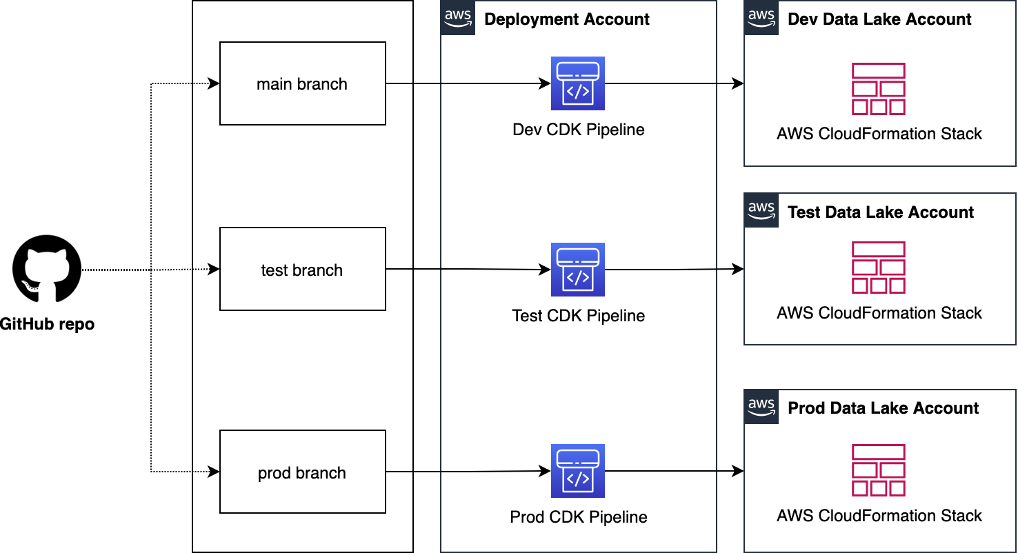
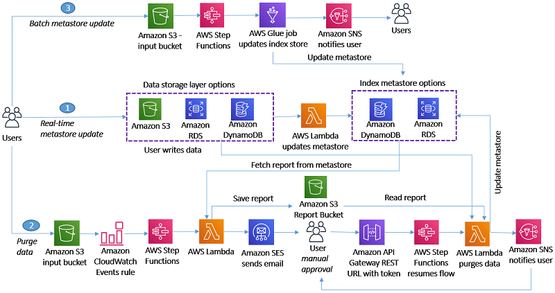
The following diagram illustrates how you can use Step Functions state machine history size to monitor and start a new Step Functions state machine run.

Step Functions Workflow

Configure the pipeline

The pipeline needs to be configured to address cost, performance, and resilience goals. You might want a pipeline that can load fresh data into the data lake and make it available quickly, and you might also want to optimize costs by loading large chunks of data into the data lake. At the same time, you should make the pipeline resilient and be able to recover in case of failures. In this section, we cover the different parameters and recommended settings to achieve these goals.

Step Functions is designed to process incoming AWS DMS CDC files by running AWS Glue jobs. AWS Glue jobs can take a couple of minutes to boot up, and when they’re running, it’s efficient to process large chunks of data. You can configure AWS DMS to write CSV files to Amazon S3 by configuring the following AWS DMS task parameters:

CdcMaxBatchInterval – Defines the maximum time limit AWS DMS will wait before writing a batch to Amazon S3
CdcMinFileSize – Defines the minimum file size AWS DMS will write to Amazon S3

Whichever condition is met first will invoke the write operation. If you want to prioritize data freshness, you should have a short CdcMaxBatchInterval value (10 seconds) and a small CdcMinFileSize value (1–5 MB). This will result in many small CSV files being written to Amazon S3 and will invoke a lot of AWS Glue jobs to process the data, making the extract, transform, and load (ETL) process faster. If you want to optimize costs, you should have a moderate CdcMaxBatchInterval (minutes) and a large CdcMinFileSize value (100–500 MB). In this scenario, we start a few AWS Glue jobs that will process large chunks of data, making the ETL flow more efficient. In a real-world use case, the required values for these parameters might fall somewhere that’s a good compromise between throughput and cost. You can configure these parameters when creating a target endpoint using the AWS DMS console, or by using the create-endpoint command in the AWS Command Line Interface (AWS CLI).

For the full list of parameters, see Using Amazon S3 as a target for AWS Database Migration Service.

Choosing the right AWS Glue worker types for the full load and CDC jobs is also crucial for performance and cost optimization. The AWS Glue (Spark) workers range from G1X to G8X, which have an increasing number of data processing units (DPUs). Full load files are usually much larger in size compared to CDC files, and therefore it’s more cost- and performance-effective to select a larger worker. For CDC files, it would be more cost-effective to select a smaller worker because files sizes are smaller.

You should design the Step Functions state machine in such a way that if anything fails, the pipeline can be redeployed after repair and resume processing from where it left off. One important parameter here is TTL for the messages in the SQS queue. This parameter defines how long a message stays in the queue before expiring. In case of failures, we want this parameter to be long enough for us to deploy a fix. Amazon SQS has a maximum of 14 days for a message’s TTL. We recommend setting this to a large enough value to minimize messages being expired in case of pipeline failures.

Clean up

Complete the following steps to clean up the resources you created in this post:

Delete the AWS Glue jobs:
1. On the AWS Glue console, choose ETL jobs in the navigation pane.
2. Select the full load and CDC jobs and on the Actions menu, choose Delete.
3. Choose Delete to confirm.
Delete the Iceberg tables:
1. On the AWS Glue console, under Data Catalog in the navigation pane, choose Databases.
2. Choose the database in which the Iceberg tables reside.
3. Select the tables to delete, choose Delete, and confirm the deletion.
Delete the S3 bucket:
1. On the Amazon S3 console, choose Buckets in the navigation pane.
2. Choose the silver bucket and empty the files in the bucket.
3. Delete the bucket.

Conclusion

In this post, we showed how to use AWS Glue jobs to load AWS DMS files into a transactional data lake framework such as Iceberg. In our setup, AWS Glue provided highly scalable and simple-to-maintain ETL jobs. Furthermore, we share a proposed solution using Step Functions to create an ETL pipeline workflow, with Amazon S3 notifications and an SQS queue to capture newly arriving files. We shared how to design this system to be resilient towards failures and to automate one of the most time-consuming tasks in maintaining a data lake: schema evolution.

In Part 3, we will share how to process the data lake to create data marts.

About the Authors

Shaheer Mansoor is a Senior Machine Learning Engineer at AWS, where he specializes in developing cutting-edge machine learning platforms. His expertise lies in creating scalable infrastructure to support advanced AI solutions. His focus areas are MLOps, feature stores, data lakes, model hosting, and generative AI.

Anoop Kumar K M is a Data Architect at AWS with focus in the data and analytics area. He helps customers in building scalable data platforms and in their enterprise data strategy. His areas of interest are data platforms, data analytics, security, file systems and operating systems. Anoop loves to travel and enjoys reading books in the crime fiction and financial domains.

Sreenivas Nettem is a Lead Database Consultant at AWS Professional Services. He has experience working with Microsoft technologies with a specialization in SQL Server. He works closely with customers to help migrate and modernize their databases to AWS.

Unleash deeper insights with Amazon Redshift data sharing for data lake tables

2024-10-10 Mohammed Alkateb

Post Syndicated from Mohammed Alkateb original https://aws.amazon.com/blogs/big-data/unleash-deeper-insights-with-amazon-redshift-data-sharing-for-data-lake-tables/

Amazon Redshift has established itself as a highly scalable, fully managed cloud data warehouse trusted by tens of thousands of customers for its superior price-performance and advanced data analytics capabilities. Driven primarily by customer feedback, the product roadmap for Amazon Redshift is designed to make sure the service continuously evolves to meet the ever-changing needs of its users.

Over the years, this customer-centric approach has led to the introduction of groundbreaking features such as zero-ETL, data sharing, streaming ingestion, data lake integration, Amazon Redshift ML, Amazon Q generative SQL, and transactional data lake capabilities. The latest innovation in Amazon Redshift data sharing capabilities further enhances the service’s flexibility and collaboration potential.

Amazon Redshift now enables the secure sharing of data lake tables—also known as external tables or Amazon Redshift Spectrum tables—that are managed in the AWS Glue Data Catalog, as well as Redshift views referencing those data lake tables. This breakthrough empowers data analytics to span the full breadth of shareable data, allowing you to seamlessly share local tables and data lake tables across warehouses, accounts, and AWS Regions—without the overhead of physical data movement or recreating security policies for data lake tables and Redshift views on each warehouse.

By using granular access controls, data sharing in Amazon Redshift helps data owners maintain tight governance over who can access the shared information. In this post, we explore powerful use cases that demonstrate how you can enhance cross-team and cross-organizational collaboration, reduce overhead, and unlock new insights by using this innovative data sharing functionality.

Overview of Amazon Redshift data sharing

Amazon Redshift data sharing allows you to securely share your data with other Redshift warehouses, without having to copy or move the data.

Data shared between warehouses doesn’t require the data to be physically copied or moved—instead, data remains in the original Redshift warehouse, and access is granted to other authorized users as part of a one-time setup. Data sharing provides granular access control, allowing you to control which specific tables or views are shared, and which users or services can access the shared data.

Since consumers access the shared data in-place, they always access the latest state of the shared data. Data sharing even allows for the automatic sharing of new tables created after that datashare was established.

You can share data across different Redshift warehouses within or across AWS accounts, and you can also do cross-region data sharing. This allows you to share data with partners, subsidiaries, or other parts of your organization, and enables the powerful workload isolation use case, as shown in the following diagram. With the seamless integration of Amazon Redshift with AWS Data Exchange, data can also be monetized and shared publicly, and public datasets such as census data can be added to a Redshift warehouse with just a few steps.

Figure 1: Amazon Redshift data sharing between producer and consumer warehouses

The data sharing capabilities in Amazon Redshift also enable the implementation of a data mesh architecture, as shown in the following diagram. This helps democratize data within the organization by reducing barriers to accessing and using data across different business units and teams. For datasets with multiple authors, Amazon Redshift data sharing supports both read and write use cases (write in preview at the time of writing). This enables the creation of 360-degree datasets, such as a customer dataset that receives contributions from multiple Redshift warehouses across different business units in the organization.

Figure 2: Data mesh architecture using Amazon Redshift data sharing

Overview of Redshift Spectrum and data lake tables

In the modern data organization, the data lake has emerged as a centralized repository—a single source of truth where all data within the organization ultimately resides at some point in its lifecycle. Redshift Spectrum enables seamless integration between the Redshift data warehouse and customers’ data lakes, as shown in the following diagram. With Redshift Spectrum, you can run SQL queries directly against data stored in Amazon Simple Storage Service (Amazon S3), without the need to first load that data into a Redshift warehouse. This allows you to maintain a comprehensive view of your data while optimizing for cost-efficiency.

Figure 3: Amazon Redshift bridges the data warehouse and data lake by enabling querying of data lake tables in-place

Redshift Spectrum supports a variety of open file formats, including Parquet, ORC, JSON, and CSV, as well as open table formats such as Apache Iceberg, all stored in Amazon S3. It runs these queries using a dedicated fleet of high-performance servers with low-latency connections to the S3 data lake. Data lake tables can be added to a Redshift warehouse either automatically through the Data Catalog, in the Amazon Redshift Query Editor, or manually using SQL commands.

From a user experience standpoint, there is little difference between querying a local Redshift table vs. a data lake table. SQL queries can be reused verbatim to perform the same aggregations and transformations on data residing in the data lake, as shown in the following examples. Additionally, by using columnar file formats like Parquet and pushing down query predicates, you can achieve further performance enhancements.

The following SQL is for a sample query against local Redshift tables:

SELECT top 10 mylocal_schema.sales.eventid, sum(mylocal_schema.sales.pricepaid) FROM mylocal_schema.sales, event
WHERE mylocal_schema.sales.eventid = event.eventid
AND mylocal_schema.sales.pricepaid > 30
GROUP BY mylocal_schema.sales.eventid
ORDER BY 2 DESC;

The following SQL is for the same query, but against data lake tables:

SELECT top 10 myspectrum_schema.sales.eventid, sum(myspectrum_schema.sales.pricepaid) FROM myspectrum_schema.sales, event
WHERE myspectrum_schema.sales.eventid = event.eventid
AND myspectrum_schema.sales.pricepaid > 30
GROUP BY myspectrum_schema.sales.eventid
ORDER BY 2 desc;

To maintain robust data governance, Redshift Spectrum integrates with AWS Lake Formation, enabling the consistent application of security policies and access controls across both the Redshift data warehouse and S3 data lake. When Lake Formation is used, Redshift producer warehouses first share their data with Lake Formation rather than directly with other Redshift consumer warehouses, and the data lake administrator grants fine-grained permissions for Redshift consumer warehouses to access the shared data. For more information, see Centrally manage access and permissions for Amazon Redshift data sharing with AWS Lake Formation.

In the past, however, sharing data lake tables across Redshift warehouses presented challenges. It wasn’t possible to do so without having to mount the data lake tables on each individual Redshift warehouse and then recreate the related security policies.

This barrier has now been addressed with the introduction of data sharing support for data lake tables. You can now share data lake tables just like any other table, using the built-in data sharing capabilities of Amazon Redshift. By combining the power of Redshift Spectrum data lake integration with the flexibility of Amazon Redshift data sharing, organizations can unlock new levels of cross-team collaboration and insights, while maintaining robust data governance and security controls.

For more information about Redshift Spectrum, see Getting started with Amazon Redshift Spectrum.

Solution overview

In this post, we describe how to add data lake tables or views to a Redshift datashare, covering two key use cases:

Adding a late-binding view or materialized view to a producer datashare that references a data lake table
Adding a data lake table directly to a producer datashare

The first use case provides greater flexibility and convenience. Consumers can query the shared view without having to configure fine-grained permissions. The configuration, such as defining permissions on data stored in Amazon S3 with Lake Formation, is already handled on the producer side. You only need to add the view to the producer datashare one time, making it a convenient option for both the producer and the consumer.

An additional benefit of this approach is that you can add views to a datashare that join data lake tables with local Redshift tables. When these views are shared, you can relegate the trusted business logic to just the producer side.

Alternatively, you can add data lake tables directly to a datashare. In this case, consumers can query the data lake tables directly or join them with their own local tables, allowing them to add their own conditional logic as needed.

Add a view that references a data lake table to a Redshift datashare

When you create data lake tables that you intend to add to a datashare, the recommended and most common way to do this is to add a view to the datashare that references a data lake table or tables. There are three high-level steps involved:

Add the Redshift view’s schema (the local schema) to the Redshift datashare.
Add the Redshift view (the local view) to the Redshift datashare.
Add the Redshift external schemas (for the tables referenced by the Redshift view) to the Redshift datashare.

The following diagram illustrates the full workflow.

Figure 4: Sharing data lake tables via Amazon Redshift views

The workflow consists of the following steps:

Create a data lake table on the datashare producer. For more information on creating Redshift Spectrum objects, see External schemas for Amazon Redshift Spectrum. Data lake tables to be shared can include Lake Formation registered tables and Data Catalog tables, and if using the Redshift Query Editor, these tables are automatically mounted.
Create a view on the producer that references the data lake table that you created.
Create a datashare, if one doesn’t already exist, and add objects to your datashare, including the view you created that references the data lake table. For more information, see Creating datashares and adding objects (preview).
Add the external schema of the base Redshift table to the datashare (this is true of both local base tables and data lake tables). You don’t have to add a data lake table itself to the datashare.
On the consumer, the administrator makes the view available to consumer database users.
Database consumer users can write queries to retrieve data from the shared view and join it with other tables and views on the consumer.

After these steps are complete, database consumer users with access to the datashare views can reference them in their SQL queries. The following SQL queries are examples for achieving the preceding steps.

Create a data lake table on the producer warehouse:

CREATE EXTERNAL TABLE myspectrum_db.myspectrum_schema.test (c1 INT)
stored AS parquet
location 's3://amzn-s3-demo-bucket/myfolder/';

Create a view on the producer warehouse:

CREATE VIEW mylocal_db.mylocal_schema.myspectrumview AS SELECT c1 FROM myspectrum_db.myspectrum_schema.v_test
WITH no schema binding;

Add a view to the datashare on the producer warehouse:

ALTER datashare mydatashare ADD SCHEMA mylocal_db.mylocal_schema;
ALTER datashare mydatashare ADD VIEW myspectrumview;
ALTER datashare mydatashare ADD SCHEMA myspectrum_db.myspectrum_schema;

Create a consumer datashare and grant permissions for the view in the consumer warehouse:

CREATE database myspectrum_db FROM datashare myspectrumproducer OF account '123456789012' namespace 'p1234567-8765-4321-p10987654321';
GRANT usage ON database myspectrum_db TO usernames;

Add a data lake table directly to a Redshift datashare

Adding a data lake table to a datashare is similar to adding a view. This process works well for a case where the consumers want the raw data from the data lake table and they want to write queries and join it to tables in their own data warehouse. There are two high-level steps involved:

Add the Redshift external schemas (of the data lake tables to be shared) to the Redshift datashare.
Add the data lake table (the Redshift external table) to the Redshift datashare.

The following diagram illustrates the full workflow.

Figure 5: Sharing data lake tables directly in an Amazon Redshift datashare

The workflow consists of the following steps:

Create a data lake table on the datashare producer.
Add objects to your datashare, including the data lake table you created. In this case, you don’t have any abstraction over the table.
On the consumer, the administrator makes the table available.
Database consumer users can write queries to retrieve data from the shared table and join it with other tables and views on the consumer.

The following SQL queries are examples for achieving the preceding producer steps.

Create a data lake table on the producer warehouse:

CREATE EXTERNAL TABLE myspectrum_db.myspectrum_schema.test (c1 INT)
stored AS parquet
location 's3://amzn-s3-demo-bucket/myfolder/';

Add a data lake schema and table directly to the datashare on the producer warehouse:

ALTER datashare mydatashare ADD SCHEMA myspectrum_db.myspectrum_schema;
ALTER datashare mydatashare ADD TABLE myspectrum_db.myspectrum_schema.test;

Create a consumer datashare and grant permissions for the view in the consumer warehouse:

CREATE database myspectrum_db FROM datashare myspectrumproducer OF account '123456789012' namespace 'p1234567-8765-4321-p10987654321';
GRANT usage ON database myspectrum_db TO usernames;

Security considerations for sharing data lake tables and views

Data lake tables are stored outside of Amazon Redshift, in the data lake, and may not be owned by the Redshift warehouse, but are still referenced within Amazon Redshift. This setup requires special security considerations. Data lake tables operate under the security and governance of both Amazon Redshift and the data lake. For Lake Formation registered tables specifically, the Amazon S3 resources are secured by Lake Formation and made available to consumers using the provided credentials.

The data owner of the data in the data lake tables may want to impose restrictions on which external objects can be added to a datashare. To give data owners more control over whether warehouse users can share data lake tables, you can use session tags in AWS Identity and Access Management (IAM). These tags provide additional context about the user running the queries. For more details on tagging resources, refer to Tags for AWS Identity and Access Management resources.

Audit considerations for sharing data lake tables and views

When sharing data lake objects through a datashare, there are special logging considerations to keep in mind:

Access controls – You can also use CloudTrail log data in conjunction with IAM policies to control access to shared tables, including both Redshift datashare producers and consumers. The CloudTrail logs record details about who accesses shared tables. The identifiers in the log data are available in the ExternalId field under the AssumeRole CloudTrail logs. The data owner can configure additional limitations on data access in an IAM policy by means of actions. For more information about defining data access through policies, see Access to AWS accounts owned by third parties.
Centralized access – Amazon S3 resources such as data lake tables can be registered and centrally managed with Lake Formation. After they’re registered with Lake Formation, Amazon S3 resources are secured and governed by the associated Lake Formation policies and made available using the credentials provided by Lake Formation.

Billing considerations for sharing data lake tables and views

The billing model for Redshift Spectrum differs for Amazon Redshift provisioned and serverless warehouses. For provisioned warehouses, Redshift Spectrum queries (queries involving data lake tables) are billed based on the amount of data scanned during query execution. For serverless warehouses, data lake queries are billed the same as non-data-lake queries. Storage for data lake tables is always billed to the AWS account associated with the Amazon S3 data.

In the case of datashares involving data lake tables, costs are attributed for storing and scanning data lake objects in a datashare as follows:

When a consumer queries shared objects from a data lake, the cost of scanning is billed to the consumer:
- When the consumer is a provisioned warehouse, Amazon Redshift uses Redshift Spectrum to scan the Amazon S3 data. Therefore, the Redshift Spectrum cost is billed to the consumer account.
- When the consumer is an Amazon Redshift Serverless workgroup, there is no separate charge for data lake queries.
Amazon S3 costs for storage and operations, such as listing buckets, is billed to the account that owns each S3 bucket.

For detailed information on Redshift Spectrum billing, refer to Amazon Redshift pricing and Billing for storage.

Conclusion

In this post, we explored how Amazon Redshift enhanced data sharing capabilities, including support for sharing data lake tables and Redshift views that reference those data lake tables, empower organizations to unlock the full potential of their data by bringing the full breadth of data assets in scope for advanced analytics. Organizations are now able to seamlessly share local tables and data lake tables across warehouses, accounts, and Regions.

We outlined the steps to securely share data lake tables and views that reference those data lake tables across Redshift warehouses, even those in separate AWS accounts or Regions. Additionally, we covered some considerations and best practices to keep in mind when using this innovative feature.

Sharing data lake tables and views through Amazon Redshift data sharing champions the modern, data-driven organization’s goal to democratize data access in a secure, scalable, and efficient manner. By eliminating the need for physical data movement or duplication, this capability reduces overhead and enables seamless cross-team and cross-organizational collaboration. Unleashing the full potential of your data analytics to span the full breadth of your local tables and data lake tables is just a few steps away.

For more information on Amazon Redshift data sharing and how it can benefit your organization, refer to the following resources:

Please also reach out to your AWS technical account manager or AWS account Solutions Architect. They will be happy to provide additional guidance and support.

About the Authors

Mohammed Alkateb is an Engineering Manager at Amazon Redshift. Prior to joining Amazon, Mohammed had 12 years of industry experience in query optimization and database internals as an individual contributor and engineering manager. Mohammed has 18 US patents, and he has publications in research and industrial tracks of premier database conferences including EDBT, ICDE, SIGMOD and VLDB. Mohammed holds a PhD in Computer Science from The University of Vermont, and MSc and BSc degrees in Information Systems from Cairo University.

Ramchandra Anil Kulkarni is a software development engineer who has been with Amazon Redshift for over 4 years. He is driven to develop database innovations that serve AWS customers globally. Kulkarni’s long-standing tenure and dedication to the Amazon Redshift service demonstrate his deep expertise and commitment to delivering cutting-edge database solutions that empower AWS customers worldwide.

Mark Lyons is a Principal Product Manager on the Amazon Redshift team. He works on the intersection of data lakes and data warehouses. Prior to joining AWS, Mark held product leadership roles with Dremio and Vertica. He is passionate about data analytics and empowering customers to change the world with their data.

Asser Moustafa is a Principal Worldwide Specialist Solutions Architect at AWS, based in Dallas, Texas. He partners with customers worldwide, advising them on all aspects of their data architectures, migrations, and strategic data visions to help organizations adopt cloud-based solutions, maximize the value of their data assets, modernize legacy infrastructures, and implement cutting-edge capabilities like machine learning and advanced analytics. Prior to joining AWS, Asser held various data and analytics leadership roles, completing an MBA from New York University and an MS in Computer Science from Columbia University in New York. He is passionate about empowering organizations to become truly data-driven and unlock the transformative potential of their data.

Accelerate Amazon Redshift Data Lake queries with AWS Glue Data Catalog Column Statistics

2024-10-01 Kalaiselvi Kamaraj

Post Syndicated from Kalaiselvi Kamaraj original https://aws.amazon.com/blogs/big-data/accelerate-amazon-redshift-data-lake-queries-with-column-level-statistics/

Amazon Redshift enables you to efficiently query and retrieve structured and semi-structured data from open format files in Amazon S3 data lake without having to load the data into Amazon Redshift tables. Amazon Redshift extends SQL capabilities to your data lake, enabling you to run analytical queries. Amazon Redshift supports a wide variety of tabular data formats like CSV, JSON, Parquet, ORC and open tabular formats like Apache Hudi, Linux foundation Delta Lake and Apache Iceberg.

You create Redshift external tables by defining the structure for your files, S3 location of the files and registering them as tables in an external data catalog. The external data catalog can be AWS Glue Data Catalog, the data catalog that comes with Amazon Athena, or your own Apache Hive metastore.

Over the last year, Amazon Redshift added several performance optimizations for data lake queries across multiple areas of query engine such as rewrite, planning, scan execution and consuming AWS Glue Data Catalog column statistics. To get the best performance on data lake queries with Redshift, you can use AWS Glue Data Catalog’s column statistics feature to collect statistics on Data Lake tables. For Amazon Redshift Serverless instances, you will see improved scan performance through increased parallel processing of S3 files and this happens automatically based on RPUs used.

In this post, we highlight the performance improvements we observed using industry standard TPC-DS benchmarks. Overall execution time of TPC-DS 3 TB benchmark improved by 3x. Some of the queries in our benchmark experienced up to 12x speed up.

Performance Improvements

Several performance optimizations were done over the last year to improve performance of data lake queries including the following.

Consume AWS Glue Data Catalog column statistics and tuning of Redshift optimizer to improve quality of query plans
Utilize bloom filters for partition columns
Improved scan efficiency for Amazon Redshift Serverless instances through increased parallel processing of files
Novel query rewrite rules to merge similar scans
Faster retrieval of metadata from AWS Glue Data Catalog

To understand the performance gains, we tested the performance on the industry-standard TPC-DS benchmark using 3 TB data sets and queries which represents different customer use cases. Performance was tested on a Redshift serverless data warehouse with 128 RPU. In our testing, the dataset was stored in Amazon S3 in Parquet format and AWS Glue Data Catalog was used to manage external databases and tables. Fact tables were partitioned on the date column, and each fact table consisted of approximately 2,000 partitions. All of the tables had their row count table property, numRows, set as per the spectrum query performance guidelines.

We did a baseline run on Redshift patch version (patch 172) from last year. Later, we ran all TPC-DS queries on latest patch version (patch 180) that includes all performance optimizations added over last year. Then we used AWS Glue Data Catalog’s column statistics feature to compute statistics for all the tables and measured improvements with the presence of AWS Glue Data Catalog column statistics.

Our analysis revealed that the TPC-DS 3TB Parquet benchmark saw substantial performance gains with these optimizations. Specifically, partitioned Parquet with our latest optimizations achieved 2x faster runtimes compared to the previous implementation. Enabling AWS Glue Data Catalog column statistics further improved performance by 3x versus last year. The following graph illustrates these runtime improvements for the full benchmark (all TPC-DS queries) over the past year, including the additional boost from using AWS Glue Data Catalog column statistics.

Figure 1: Improvement in total runtime of TPC-DS 3T workload

The following graph presents the top queries from the TPC-DS benchmark with the greatest performance improvement over the last year with and without AWS Glue Data Catalog column statistics. You can see that performance improves a lot when statistics exist on AWS Glue Data Catalog (for details on how to get statistics for your Data Lake tables, please refer to optimizing query performance using AWS Glue Data Catalog column statistics). Specifically, multi-join queries will benefit the most from AWS Glue Data Catalog column statistics because the optimizer uses statistics to choose the right join order and distribution strategy.

Figure 2: Speed-up in TPC-DS queries

Let’s discuss some of the optimizations that contributed to improved query performance.

Optimizing with table-level statistics

Amazon Redshift’s design enables it to handle large-scale data challenges with superior speed and cost-efficiency. Its massively parallel processing (MPP) query engine, AI-powered query optimizer, auto-scaling capabilities, and other advanced features allow Redshift to excel at searching, aggregating, and transforming petabytes of data.

However, even the most powerful systems can experience performance degradation if they encounter anti-patterns like grossly inaccurate table statistics, such as the row count metadata.

Without this crucial metadata, Redshift’s query optimizer may be limited in the number of possible optimizations, especially those related to data distribution during query execution. This can have a significant impact on overall query performance.

To illustrate this, consider the following simple query involving an inner join between a large table with billions of rows and a small table with only a few hundred thousand rows.

select small_table.sellerid, sum(large_table.qtysold)
from large_table, small_table
where large_table.salesid = small_table.listid
 and small_table.listtime > '2023-12-01'
 and large_table.saletime > '2023-12-01'
group by 1 order by 1

If executed as-is, with the large table on the right-hand side of the join, the query will lead to sub-optimal performance. This is because the large table will need to be distributed (broadcast) to all Redshift compute nodes to perform the inner join with the small table, as shown in the following diagram.

Inaccurate table statistics lead to limited optimizations and large amounts of data broadcast among compute nodes for a simple inner join

Figure 3: Inaccurate table statistics lead to limited optimizations and large amounts of data broadcast among compute nodes for a simple inner join

Now, consider a scenario where the table statistics, such as the row count, are accurate. This allows the Amazon Redshift query optimizer to make more informed decisions, such as determining the optimal join order. In this case, the optimizer would immediately rewrite the query to have the large table on the left-hand side of the inner join, so that it is the small table that is broadcast across the Redshift compute nodes, as illustrated in the following diagram.

Accurate table statistics lead to high degree of optimizations and very little data broadcast among compute nodes for a simple inner join

Figure 4: Accurate table statistics lead to high degree of optimizations and very little data broadcast among compute nodes for a simple inner join

Fortunately, Amazon Redshift automatically maintains accurate table statistics for local tables by running the ANALYZE command in the background. For external tables (data lake tables), however, AWS Glue Data Catalog column statistics are recommended for use with Amazon Redshift as we will discuss in the next section. For more general information on optimizing queries in Amazon Redshift, please refer to the documentation on factors affecting query performance, data redistribution, and Amazon Redshift best practices for designing queries.

Improvements with AWS Glue Data Catalog column statistics

AWS Glue Data Catalog has a feature to compute column level statistics for Amazon S3 backed external tables. AWS Glue Data Catalog can compute column level statistics such as NDV, Number of Nulls, Min/Max and Avg. column width for the columns without the need for additional data pipelines. Amazon Redshift cost-based optimizer utilizes these statistics to come up with better quality query plans. In addition to consuming statistics, we also made several improvements in cardinality estimations and cost tuning to get high quality query plans thereby improving query performance.

TPC-DS 3TB dataset showed 40% improvement in total query execution time when these AWS Glue Data Catalog column statistics were provided. Individual TPC-DS queries showed up to 5x improvements in query execution time. Some of the queries that had greater impact in execution time are Q85, Q64, Q75, Q78, Q94, Q16, Q04, Q24 and Q11.

We will go through an example where cost-based optimizer generated a better query plan with statistics and how it improved the execution time.

Let’s consider following simpler version of TPC-DS Q64 to showcase the query plan differences with statistics.

select i_product_name product_name
,i_item_sk item_sk
,ad1.ca_street_number b_street_number
,ad1.ca_street_name b_street_name
,ad1.ca_city b_city
,ad1.ca_zip b_zip
,d1.d_year as syear
,count(*) cnt
,sum(ss_wholesale_cost) s1
,sum(ss_list_price) s2
,sum(ss_coupon_amt) s3
FROM   tpcds_3t_alls3_pp_ext.store_sales
,tpcds_3t_alls3_pp_ext.store_returns
,tpcds_3t_alls3_pp_ext.date_dim d1
,tpcds_3t_alls3_pp_ext.customer
,tpcds_3t_alls3_pp_ext.customer_address ad1
,tpcds_3t_alls3_pp_ext.item
WHERE
ss_sold_date_sk = d1.d_date_sk AND
ss_customer_sk = c_customer_sk AND

ss_addr_sk = ad1.ca_address_sk and
ss_item_sk = i_item_sk and
ss_item_sk = sr_item_sk and
ss_ticket_number = sr_ticket_number and
i_color in ('firebrick','papaya','orange','cream','turquoise','deep') and
i_current_price between 42 and 42 + 10 and
i_current_price between 42 + 1 and 42 + 15
group by i_product_name
,i_item_sk
,ad1.ca_street_number
,ad1.ca_street_name
,ad1.ca_city
,ad1.ca_zip
,d1.d_year

Without Statistics

Following figure represents the logical query plan of Q64. You can observe that cardinality estimation of joins is not accurate. With inaccurate cardinalities, optimizer produces a sub-optimal query plan leading to higher execution time.

With Statistics

Following figure represents the logical query plan after consuming AWS Glue Data Catalog column statistics. Based on the highlighted changes, you can observe that the cardinality estimations of JOIN improved by many magnitudes helping the optimizer to choose a better join order and join strategy (broadcast DS_BCAST_INNER vs. distribute DS_DIST_BOTH). Switching the customer_address and customer table from inner to outer table and making join strategies as distribute has major impact because this reduces the data movement between the nodes and avoids spilling from hash table.

Figure 5: Logical query plan of Q64 without statistics

Logical query plan of Q64 after consuming column-level statistics

Figure 6: Logical query plan of Q64 after consuming AWS Glue Data Catalog column statistics

This change in query plan improved the query execution time of Q64 from 383s to 81s.

Given the greater benefits with AWS Glue Data Catalog column statistics for the optimizer, you should consider collecting stats for your data lake using AWS Glue. If your workload is a JOIN heavy workload, then collecting stats will show greater improvement on your workload. Refer to generating AWS Glue Data Catalog column statistics for instructions on how to collect statistics in AWS Glue Data Catalog.

Query rewrite optimization

We introduced a new query rewrite rule which combines scalar aggregates over the same common expression using slightly different predicates. This rewrite resulted in performance improvements on TPC-DS queries Q09, Q28, and Q88. Let’s focus on Q09 as a representative of these queries, given by the following fragment:

SELECT CASE
WHEN (SELECT COUNT(*)
FROM store_sales
WHERE ss_quantity BETWEEN 1 AND 20) > 48409437
THEN (SELECT AVG(ss_ext_discount_amt)
FROM store_sales
WHERE ss_quantity BETWEEN 1 AND 20)
ELSE (SELECT AVG(ss_net_profit)
FROM store_sales
WHERE ss_quantity BETWEEN 1 AND 20) END
AS bucket1,
<<4 more variations of the CASE expression above>>
FROM reason
WHERE r_reason_sk = 1

In total, there are 15 scans of the fact table store_sales, each one returning various aggregates over different subsets of data. The engine first performs subquery removal and transforms the various expressions in the CASE statements into relational subtrees connected via cross products, and then they are fused into one subquery handling all scalar aggregates. The resulting plan for Q09, described below using SQL for clarity, is given by:

SELECT CASE WHEN v1 > 48409437 THEN t1 ELSE e1 END,
<4 more variations>
FROM (SELECT COUNT(CASE WHEN b1 THEN 1 END) AS v1,
AVG(CASE WHEN b1 THEN ss_ext_discount_amt END) AS t1,
AVG(CASE WHEN b1 THEN ss_net_profit END) AS e1,
<4 more variations>
FROM reason,
(SELECT *,
ss_quantity BETWEEN 1 AND 20 AS b1,
<4 more variations>
FROM store_sales
WHERE ss_quantity BETWEEN 1 AND 20 OR
<4 more variations>))
WHERE r_reason_sk = 1)

In general, this rewrite rule results in the largest improvements both in latency (from 3x to 8x improvements) and bytes read from Amazon S3 (from 6x to 8x reduction in scanned bytes and, consequently, cost).

Bloom filter for partition columns

Amazon Redshift already uses Bloom filters on data columns of external tables in Amazon S3 to enable early and effective data filtering. Last year, we extended this support for partition columns as well. A Bloom filter is a probabilistic, memory-efficient data structure that accelerates join queries at scale by filtering rows that do not match the join relation, significantly reducing the amount of data transferred over the network. Amazon Redshift automatically determines what queries are suitable for leveraging Bloom filters at query runtime.

This optimization resulted in performance improvements on TPC-DS queries Q05, Q17 and Q54. This optimization resulted in large improvements in both latency (from 2x to 3x improvement) and bytes read from S3 (from 9x to 15x reduction in scanned bytes and, consequently cost).

Following is the subquery of Q05 which showcased improvements with runtime filter.

select s_store_id,
sum(sales_price) as sales,
sum(profit) as profit,
sum(return_amt) as returns,
sum(net_loss) as profit_loss
from
( select  ss_store_sk as store_sk,
ss_sold_date_sk  as date_sk,
ss_ext_sales_price as sales_price,
ss_net_profit as profit,
cast(0 as decimal(7,2)) as return_amt,
cast(0 as decimal(7,2)) as net_loss
from tpcds_3t_alls3_pp_ext.store_sales
union all
select sr_store_sk as store_sk,
sr_returned_date_sk as date_sk,
cast(0 as decimal(7,2)) as sales_price,
cast(0 as decimal(7,2)) as profit,
sr_return_amt as return_amt,
sr_net_loss as net_loss
from tpcds_3t_alls3_pp_ext.store_returns
) salesreturnss,
tpcds_3t_alls3_pp_ext.date_dim,
tpcds_3t_alls3_pp_ext.store
where date_sk = d_date_sk
and d_date between cast('1998-08-13' as date)
and (cast('1998-08-13' as date) +  14)
and store_sk = s_store_sk
group by s_store_id

Without bloom filter support on partition columns

Following figure is the logical query plan for sub-query of Q05. This appends two large fact tables store_sales (8B rows) and store_returns (863M rows) and then joins with very selective dimension tables date_dim and then with dimension table store. You can observe that join with date_dim table reduces the number of rows from 9B to 93M rows.

With bloom filter support on partition columns

With support of bloom filter on partition columns, we now create bloom filter for d_date_sk column of date_dim table and push down the bloom filters to store_sales and store_returns table. These bloom filters help to filter out the partitions in both store_sales and store_returns table because join happens on partition column (number of partitions processed reduces by 10x).

Figure 7: Logical query plan for sub-query of Q05 without bloom filter support on partition columns

Figure 8: Logical query plan for sub-query of Q05 with bloom filter support on partition columns

Overall, bloom filter on partition column will reduce the number of partitions processed resulting in reduced S3 listing calls and lesser number of data files to be read (reduction in scanned bytes). You can see that we only scan 89M rows from store_sales and 4M rows from store_returns because of the bloom filter. This reduced number of rows to process at JOIN level and helped in improving the overall query performance by 2x and scanned bytes by 9x.

Conclusion

In this post, we covered new performance optimizations in Amazon Redshift data lake query processing and how AWS Glue Data Catalog statistics helps to enhance quality of query plans for data lake queries in Amazon Redshift. These optimizations together improved TPC-DS 3 TB benchmark by 3x. Some of the queries in our benchmark benefited up to 12x speed up.

In summary, Amazon Redshift now offers enhanced query performance with optimizations such as AWS Glue Data Catalog column statistics, bloom filters on partition columns, new query rewrite rules and faster retrieval of metadata. These optimizations are enabled by default and Amazon Redshift users will benefit with better query response times for their workloads. For more information, please reach out to your AWS technical account manager or AWS account solutions architect. They will be happy to provide additional guidance and support.

About the authors

Kalaiselvi Kamaraj is a Sr. Software Development Engineer with Amazon. She has worked on several projects within Redshift Query processing team and currently focusing on performance related projects for Redshift Data Lake.

Asser Moustafa is a Principal Worldwide Specialist Solutions Architect at AWS, based in Dallas, Texas, USA. He partners with customers worldwide, advising them on all aspects of their data architectures, migrations, and strategic data visions to help organizations adopt cloud-based solutions, maximize the value of their data assets, modernize legacy infrastructures, and implement cutting-edge capabilities like machine learning and advanced analytics. Prior to joining AWS, Asser held various data and analytics leadership roles, completing an MBA from New York University and an MS in Computer Science from Columbia University in New York. He is passionate about empowering organizations to become truly data-driven and unlock the transformative potential of their data.

Empower your Jira data in a data lake with Amazon AppFlow and AWS Glue

2023-08-01 Tom Romano

Post Syndicated from Tom Romano original https://aws.amazon.com/blogs/big-data/empower-your-jira-data-in-a-data-lake-with-amazon-appflow-and-aws-glue/

In the world of software engineering and development, organizations use project management tools like Atlassian Jira Cloud. Managing projects with Jira leads to rich datasets, which can provide historical and predictive insights about project and development efforts.

Although Jira Cloud provides reporting capability, loading this data into a data lake will facilitate enrichment with other business data, as well as support the use of business intelligence (BI) tools and artificial intelligence (AI) and machine learning (ML) applications. Companies often take a data lake approach to their analytics, bringing data from many different systems into one place to simplify how the analytics are done.

This post shows you how to use Amazon AppFlow and AWS Glue to create a fully automated data ingestion pipeline that will synchronize your Jira data into your data lake. Amazon AppFlow provides software as a service (SaaS) integration with Jira Cloud to load the data into your AWS account. AWS Glue is a serverless data discovery, load, and transformation service that will prepare data for consumption in BI and AI/ML activities. Additionally, this post strives to achieve a low-code and serverless solution for operational efficiency and cost optimization, and the solution supports incremental loading for cost optimization.

Solution overview

This solution uses Amazon AppFlow to retrieve data from the Jira Cloud. The data is synchronized to an Amazon Simple Storage Service (Amazon S3) bucket using an initial full download and subsequent incremental downloads of changes. When new data arrives in the S3 bucket, an AWS Step Functions workflow is triggered that orchestrates extract, transform, and load (ETL) activities using AWS Glue crawlers and AWS Glue DataBrew. The data is then available in the AWS Glue Data Catalog and can be queried by services such as Amazon Athena, Amazon QuickSight, and Amazon Redshift Spectrum. The solution is completely automated and serverless, resulting in low operational overhead. When this setup is complete, your Jira data will be automatically ingested and kept up to date in your data lake!

The following diagram illustrates the solution architecture.

The Jira Appflow Architecture is shown. The Jira Cloud data is retrieved by Amazon AppFlow and is stored in Amazon S3. This triggers an Amazon EventBridge event that runs an AWS Step Functions workflow. The workflow uses AWS Glue to catalog and transform the data, The data is then queried with QuickSight.

The Step Functions workflow orchestrates the following ETL activities, resulting in two tables:

An AWS Glue crawler collects all downloads into a single AWS Glue table named jira_raw. This table is comprised of a mix of full and incremental downloads from Jira, with many versions of the same records representing changes over time.
A DataBrew job prepares the data for reporting by unpacking key-value pairs in the fields, as well as removing depreciated records as they are updated in subsequent change data captures. This reporting-ready data will available in an AWS Glue table named jira_data.

The following figure shows the Step Functions workflow.

A diagram represents the AWS Step Functions workflow. It contains the steps to run an AWS Crawler, wait for it's completion, and then run a AWS Glue DataBrew data transformation job.

Prerequisites

This solution requires the following:

Administrative access to your Jira Cloud instance, and an associated Jira Cloud developer account.
An AWS account and a login with access to the AWS Management Console. Your login will need AWS Identity and Access Management (IAM) permissions to create and access the resources in your AWS account.
Basic knowledge of AWS and working knowledge of Jira administration.

Configure the Jira Instance

After logging in to your Jira Cloud instance, you establish a Jira project with associated epics and issues to download into a data lake. If you’re starting with a new Jira instance, it helps to have at least one project with a sampling of epics and issues for the initial data download, because it allows you to create an initial dataset without errors or missing fields. Note that you may have multiple projects as well.

An image show a Jira Cloud example, with several issues arranged in a Kansan board.

After you have established your Jira project and populated it with epics and issues, ensure you also have access to the Jira developer portal. In later steps, you use this developer portal to establish authentication and permissions for the Amazon AppFlow connection.

Provision resources with AWS CloudFormation

For the initial setup, you launch an AWS CloudFormation stack to create an S3 bucket to store data, IAM roles for data access, and the AWS Glue crawler and Data Catalog components. Complete the following steps:

Sign in to your AWS account.
Click Launch Stack:
For Stack name, enter a name for the stack (the default is aws-blog-jira-datalake-with-AppFlow).
For GlueDatabaseName, enter a unique name for the Data Catalog database to hold the Jira data table metadata (the default is jiralake).
For InitialRunFlag, choose Setup. This mode will scan all data and disable the change data capture (CDC) features of the stack. (Because this is the initial load, the stack needs an initial data load before you configure CDC in later steps.)
Under Capabilities and transforms, select the acknowledgement check boxes to allow IAM resources to be created within your AWS account.
Review the parameters and choose Create stack to deploy the CloudFormation stack. This process will take around 5–10 minutes to complete.
After the stack is deployed, review the Outputs tab for the stack and collect the following values to use when you set up Amazon AppFlow:
- Amazon AppFlow destination bucket (o01AppFlowBucket)
- Amazon AppFlow destination bucket path (o02AppFlowPath)
- Role for Amazon AppFlow Jira connector (o03AppFlowRole)

Configure Jira Cloud

Next, you configure your Jira Cloud instance for access by Amazon AppFlow. For full instructions, refer to Jira Cloud connector for Amazon AppFlow. The following steps summarize these instructions and discuss the specific configuration to enable OAuth in the Jira Cloud:

Open the Jira developer portal.
Create the OAuth 2 integration from the developer application console by choosing Create an OAuth 2.0 Integration. This will provide a login mechanism for AppFlow.
Enable fine-grained permissions. See Recommended scopes for the permission settings to grant AppFlow appropriate access to your Jira instance.
Add the following permission scopes to your OAuth app:
1. manage:jira-configuration
2. read:field-configuration:jira
Under Authorization, set the Call Back URL to return to Amazon AppFlow with the URL https://us-east-1.console.aws.amazon.com/AppFlow/oauth.
Under Settings, note the client ID and secret to use in later steps to set up authentication from Amazon AppFlow.

Create the Amazon AppFlow Jira Cloud connection

In this step, you configure Amazon AppFlow to run a one-time full data fetch of all your data, establishing the initial data lake:

On the Amazon AppFlow console, choose Connectors in the navigation pane.
Search for the Jira Cloud connector.
Choose Create flow on the connector tile to create the connection to your Jira instance.
For Flow name, enter a name for the flow (for example, JiraLakeFlow).
Leave the Data encryption setting as the default.
Choose Next.
For Source name, keep the default of Jira Cloud.
Choose Create new connection under Jira Cloud connection.
In the Connect to Jira Cloud section, enter the values for Client ID, Client secret, and Jira Cloud Site that you collected earlier. This provides the authentication from AppFlow to Jira Cloud.
For Connection Name, enter a connection name (for example, JiraLakeCloudConnection).
Choose Connect. You will be prompted to allow your OAuth app to access your Atlassian account to verify authentication.
In the Authorize App window that pops up, choose Accept.
With the connection created, return to the Configure flow section on the Amazon AppFlow console.
For API version, choose V2 to use the latest Jira query API.
For Jira Cloud object, choose Issue to query and download all issues and associated details.
For Destination Name in the Destination Details section, choose Amazon S3.
For Bucket details, choose the S3 bucket name that matches the Amazon AppFlow destination bucket value that you collected from the outputs of the CloudFormation stack.
Enter the Amazon AppFlow destination bucket path to complete the full S3 path. This will send the Jira data to the S3 bucket created by the CloudFormation script.
Leave Catalog your data in the AWS Glue Data Catalog unselected. The CloudFormation script uses an AWS Glue crawler to update the Data Catalog in a different manner, grouping all the downloads into a common table, so we disable the update here.
For File format settings, select Parquet format and select Preserve source data types in Parquet output. Parquet is a columnar format to optimize subsequent querying.
Select Add a timestamp to the file name for Filename preference. This will allow you to easily find data files downloaded at a specific date and time.
For now, select Run on Demand for the Flow trigger to run the full load flow manually. You will schedule downloads in a later step when implementing CDC.
Choose Next.
On the Map data fields page, select Manually map fields.
For Source to destination field mapping, choose the drop-down box under Source field name and select Map all fields directly. This will bring down all fields as they are received, because we will instead implement data preparation in later steps.
Under Partition and aggregation settings, you can set up the partitions in a way that works for your use case. For this example, we use a daily partition, so select Date and time and choose Daily.
For Aggregation settings, leave it as the default of Don’t aggregate.
Choose Next.
On the Add filters page, you can create filters to only download specific data. For this example, you download all the data, so choose Next.
Review and choose Create flow.
When the flow is created, choose Run flow to start the initial data seeding. After some time, you should receive a banner indicating the run finished successfully.

Review seed data

At this stage in the process, you now have data in your S3 environment. When new data files are created in the S3 bucket, it will automatically run an AWS Glue crawler to catalog the new data. You can see if it’s complete by reviewing the Step Functions state machine for a Succeeded run status. There is a link to the state machine on the CloudFormation stack’s Resources tab, which will redirect you to the Step Functions state machine.

A image showing the CloudFormation resources tab of the stack, with a link to the AWS Step Functions workflow.

When the state machine is complete, it’s time to review the raw Jira data with Athena. The database is as you specified in the CloudFormation stack (jiralake by default), and the table name is jira_raw. If you kept the default AWS Glue database name of jiralake, the Athena SQL is as follows:

SELECT * FROM "jiralake"."jira_raw" limit 10;

If you explore the data, you’ll notice that most of the data you would want to work with is actually packed into a column called fields. This means the data is not available as columns in your Athena queries, making it harder to select, filter, and sort individual fields within an Athena SQL query. This will be addressed in the next steps.

An image demonstrating the Amazon Athena query SELECT * FROM "jiralake"."jira_raw" limit 10;

Set up CDC and unpack the fields columns

To add the ongoing CDC and reformat the data for analytics, we introduce a DataBrew job to transform the data and filter to the most recent version of each record as changes come in. You can do this by updating the CloudFormation stack with a flag that includes the CDC and data transformation steps.

On the AWS CloudFormation console, return to the stack.
Choose Update.
Select Use current template and choose Next.
For SetupOrCDC, choose CDC, then choose Next. This will enable both the CDC steps and the data transformation steps for the Jira data.
Continue choosing Next until you reach the Review section.
Select I acknowledge that AWS CloudFormation might create IAM resources, then choose Submit.
Return to the Amazon AppFlow console and open your flow.
On the Actions menu, choose Edit flow. We will now edit the flow trigger to run an incremental load on a periodic basis.
Select Run flow on schedule.
Configure the desired repeats, as well as start time and date. For this example, we choose Daily for Repeats and enter 1 for the number of days you’ll have the flow trigger. For Starting at, enter 01:00.
Select Incremental transfer for Transfer mode.
Choose Updated on the drop-down menu so that changes will be captured based on when the records were updated.
Choose Save. With these settings in our example, the run will happen nightly at 1:00 AM.

Review the analytics data

When the next incremental load occurs that results in new data, the Step Functions workflow will start the DataBrew job and populate a new staged analytical data table named jira_data in your Data Catalog database. If you don’t want to wait, you can trigger the Step Functions workflow manually.

The DataBrew job performs data transformation and filtering tasks. The job unpacks the key-values from the Jira JSON data and the raw Jira data, resulting in a tabular data schema that facilitates use with BI and AI/ML tools. As Jira items are changed, the changed item’s data is resent, resulting in multiple versions of an item in the raw data feed. The DataBrew job filters the raw data feed so that the resulting data table only contains the most recent version of each item. You could enhance this DataBrew job to further customize the data for your needs, such as renaming the generic Jira custom field names to reflect their business meaning.

When the Step Functions workflow is complete, we can query the data in Athena again using the following query:

SELECT * FROM "jiralake"."jira_data" limit 10;

You can see that in our transformed jira_data table, the nested JSON fields are broken out into their own columns for each field. You will also notice that we’ve filtered out obsolete records that have been superseded by more recent record updates in later data loads so the data is fresh. If you want to rename custom fields, remove columns, or restructure what comes out of the nested JSON, you can modify the DataBrew recipe to accomplish this. At this point, the data is ready to be used by your analytics tools, such as Amazon QuickSight.

An image demonstrating the Amazon Athena query SELECT * FROM "jiralake"."jira_data" limit 10;

Clean up

If you would like to discontinue this solution, you can remove it with the following steps:

On the Amazon AppFlow console, deactivate the flow for Jira, and optionally delete it.
On the Amazon S3 console, select the S3 bucket for the stack, and empty the bucket to delete the existing data.
On the AWS CloudFormation console, delete the CloudFormation stack that you deployed.

Conclusion

In this post, we created a serverless incremental data load process for Jira that will synchronize data while handling custom fields using Amazon AppFlow, AWS Glue, and Step Functions. The approach uses Amazon AppFlow to incrementally load the data into Amazon S3. We then use AWS Glue and Step Functions to manage the extraction of the Jira custom fields and load them in a format to be queried by analytics services such as Athena, QuickSight, or Redshift Spectrum, or AI/ML services like Amazon SageMaker.

To learn more about AWS Glue and DataBrew, refer to Getting started with AWS Glue DataBrew. With DataBrew, you can take the sample data transformation in this project and customize the output to meet your specific needs. This could include renaming columns, creating additional fields, and more.

To learn more about Amazon AppFlow, refer to Getting started with Amazon AppFlow. Note that Amazon AppFlow supports integrations with many SaaS applications in addition to the Jira Cloud.

To learn more about orchestrating flows with Step Functions, see Create a Serverless Workflow with AWS Step Functions and AWS Lambda. The workflow could be enhanced to load the data into a data warehouse, such as Amazon Redshift, or trigger a refresh of a QuickSight dataset for analytics and reporting.

In future posts, we will cover how to unnest parent-child relationships within the Jira data using Athena and how to visualize the data using QuickSight.

About the Authors

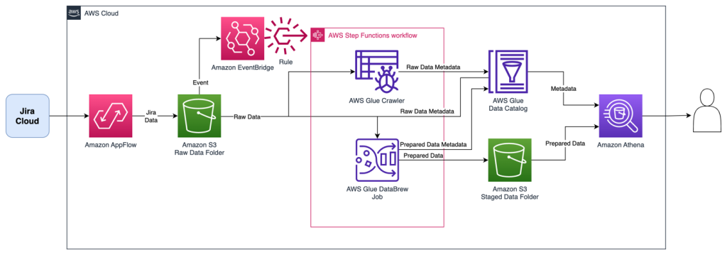
Tom Romano is a Sr. Solutions Architect for AWS World Wide Public Sector from Tampa, FL, and assists GovTech and EdTech customers as they create new solutions that are cloud native, event driven, and serverless. He is an enthusiastic Python programmer for both application development and data analytics, and is an Analytics Specialist. In his free time, Tom flies remote control model airplanes and enjoys vacationing with his family around Florida and the Caribbean.

Shane Thompson is a Sr. Solutions Architect based out of San Luis Obispo, California, working with AWS Startups. He works with customers who use AI/ML in their business model and is passionate about democratizing AI/ML so that all customers can benefit from it. In his free time, Shane loves to spend time with his family and travel around the world.

Build a semantic search engine for tabular columns with Transformers and Amazon OpenSearch Service

2023-03-01 Kachi Odoemene

Post Syndicated from Kachi Odoemene original https://aws.amazon.com/blogs/big-data/build-a-semantic-search-engine-for-tabular-columns-with-transformers-and-amazon-opensearch-service/

Finding similar columns in a data lake has important applications in data cleaning and annotation, schema matching, data discovery, and analytics across multiple data sources. The inability to accurately find and analyze data from disparate sources represents a potential efficiency killer for everyone from data scientists, medical researchers, academics, to financial and government analysts.

Conventional solutions involve lexical keyword search or regular expression matching, which are susceptible to data quality issues such as absent column names or different column naming conventions across diverse datasets (for example, zip_code, zcode, postalcode).

In this post, we demonstrate a solution for searching for similar columns based on column name, column content, or both. The solution uses approximate nearest neighbors algorithms available in Amazon OpenSearch Service to search for semantically similar columns. To facilitate the search, we create features representations (embeddings) for individual columns in the data lake using pre-trained Transformer models from the sentence-transformers library in Amazon SageMaker. Finally, to interact with and visualize results from our solution, we build an interactive Streamlit web application running on AWS Fargate.

We include a code tutorial for you to deploy the resources to run the solution on sample data or your own data.

Solution overview

The following architecture diagram illustrates the two-stage workflow for finding semantically similar columns. The first stage runs an AWS Step Functions workflow that creates embeddings from tabular columns and builds the OpenSearch Service search index. The second stage, or the online inference stage, runs a Streamlit application through Fargate. The web application collects input search queries and retrieves from the OpenSearch Service index the approximate k-most-similar columns to the query.

Figure 1. Solution architecture

The automated workflow proceeds in the following steps:

The user uploads tabular datasets into an Amazon Simple Storage Service (Amazon S3) bucket, which invokes an AWS Lambda function that initiates the Step Functions workflow.
The workflow begins with an AWS Glue job that converts the CSV files into Apache Parquet data format.
A SageMaker Processing job creates embeddings for each column using pre-trained models or custom column embedding models. The SageMaker Processing job saves the column embeddings for each table in Amazon S3.
A Lambda function creates the OpenSearch Service domain and cluster to index the column embeddings produced in the previous step.
Finally, an interactive Streamlit web application is deployed with Fargate. The web application provides an interface for the user to input queries to search the OpenSearch Service domain for similar columns.

You can download the code tutorial from GitHub to try this solution on sample data or your own data. Instructions on the how to deploy the required resources for this tutorial are available on Github.

Prerequistes

To implement this solution, you need the following:

An AWS account.
Basic familiarity with AWS services such as the AWS Cloud Development Kit (AWS CDK), Lambda, OpenSearch Service, and SageMaker Processing.
A tabular dataset to create the search index. You can bring your own tabular data or download the sample datasets on GitHub.

Build a search index

The first stage builds the column search engine index. The following figure illustrates the Step Functions workflow that runs this stage.

Figure 2 – Step functions workflow – multiple embedding models

Datasets

In this post, we build a search index to include over 400 columns from over 25 tabular datasets. The datasets originate from the following public sources:

s3://sagemaker-sample-files/datasets/tabular/
NYC Open Data
Chicago Data Portal

For the the full list of the tables included in the index, see the code tutorial on GitHub.

You can bring your own tabular dataset to augment the sample data or build your own search index. We include two Lambda functions that initiate the Step Functions workflow to build the search index for individual CSV files or a batch of CSV files, respectively.

Transform CSV to Parquet

Raw CSV files are converted to Parquet data format with AWS Glue. Parquet is a column-oriented format file format preferred in big data analytics that provides efficient compression and encoding. In our experiments, the Parquet data format offered significant reduction in storage size compared to raw CSV files. We also used Parquet as a common data format to convert other data formats (for example JSON and NDJSON) because it supports advanced nested data structures.

Create tabular column embeddings

To extract embeddings for individual table columns in the sample tabular datasets in this post, we use the following pre-trained models from the sentence-transformers library. For additional models, see Pretrained Models.

Model name	Dimension	Size (MB)
all-MiniLM-L6-v2	384	80
all-distilroberta-v1	768	290
average_word_embeddings_glove.6B.300d	300	420

The SageMaker Processing job runs create_embeddings.py(code) for a single model. For extracting embeddings from multiple models, the workflow runs parallel SageMaker Processing jobs as shown in the Step Functions workflow. We use the model to create two sets of embeddings:

column_name_embeddings – Embeddings of column names (headers)
column_content_embeddings – Average embedding of all the rows in the column

For more information about the column embedding process, see the code tutorial on GitHub.

An alternative to the SageMaker Processing step is to create a SageMaker batch transform to get column embeddings on large datasets. This would require deploying the model to a SageMaker endpoint. For more information, see Use Batch Transform.

Index embeddings with OpenSearch Service

In the final step of this stage, a Lambda function adds the column embeddings to a OpenSearch Service approximate k-Nearest-Neighbor (kNN) search index. Each model is assigned its own search index. For more information about the approximate kNN search index parameters, see k-NN.

Online inference and semantic search with a web app

The second stage of the workflow runs a Streamlit web application where you can provide inputs and search for semantically similar columns indexed in OpenSearch Service. The application layer uses an Application Load Balancer, Fargate, and Lambda. The application infrastructure is automatically deployed as part of the solution.

The application allows you to provide an input and search for semantically similar column names, column content, or both. Additionally, you can select the embedding model and number of nearest neighbors to return from the search. The application receives inputs, embeds the input with the specified model, and uses kNN search in OpenSearch Service to search indexed column embeddings and find the most similar columns to the given input. The search results displayed include the table names, column names, and similarity scores for the columns identified, as well as the locations of the data in Amazon S3 for further exploration.

The following figure shows an example of the web application. In this example, we searched for columns in our data lake that have similar Column Names (payload type) to district (payload). The application used all-MiniLM-L6-v2 as the embedding model and returned 10 (k) nearest neighbors from our OpenSearch Service index.

The application returned transit_district, city, borough, and location as the four most similar columns based on the data indexed in OpenSearch Service. This example demonstrates the ability of the search approach to identify semantically similar columns across datasets.

Figure 3: Web application user interface

Clean up

To delete the resources created by the AWS CDK in this tutorial, run the following command:

cdk destroy --all

Conclusion

In this post, we presented an end-to-end workflow for building a semantic search engine for tabular columns.

Get started today on your own data with our code tutorial available on GitHub. If you’d like help accelerating your use of ML in your products and processes, please contact the Amazon Machine Learning Solutions Lab.

About the Authors

Kachi Odoemene is an Applied Scientist at AWS AI. He builds AI/ML solutions to solve business problems for AWS customers.

Taylor McNally is a Deep Learning Architect at Amazon Machine Learning Solutions Lab. He helps customers from various industries build solutions leveraging AI/ML on AWS. He enjoys a good cup of coffee, the outdoors, and time with his family and energetic dog.

Austin Welch is a Data Scientist in the Amazon ML Solutions Lab. He develops custom deep learning models to help AWS public sector customers accelerate their AI and cloud adoption. In his spare time, he enjoys reading, traveling, and jiu-jitsu.

Automate replication of relational sources into a transactional data lake with Apache Iceberg and AWS Glue

2023-02-14 Luis Gerardo Baeza

Post Syndicated from Luis Gerardo Baeza original https://aws.amazon.com/blogs/big-data/automate-replication-of-relational-sources-into-a-transactional-data-lake-with-apache-iceberg-and-aws-glue/

Organizations have chosen to build data lakes on top of Amazon Simple Storage Service (Amazon S3) for many years. A data lake is the most popular choice for organizations to store all their organizational data generated by different teams, across business domains, from all different formats, and even over history. According to a study, the average company is seeing the volume of their data growing at a rate that exceeds 50% per year, usually managing an average of 33 unique data sources for analysis.

Teams often try to replicate thousands of jobs from relational databases with the same extract, transform, and load (ETL) pattern. There is lot of effort in maintaining the job states and scheduling these individual jobs. This approach helps the teams add tables with few changes and also maintains the job status with minimum effort. This can lead to a huge improvement in the development timeline and tracking the jobs with ease.

In this post, we show you how to easily replicate all your relational data stores into a transactional data lake in an automated fashion with a single ETL job using Apache Iceberg and AWS Glue.

Solution architecture

Data lakes are usually organized using separate S3 buckets for three layers of data: the raw layer containing data in its original form, the stage layer containing intermediate processed data optimized for consumption, and the analytics layer containing aggregated data for specific use cases. In the raw layer, tables usually are organized based on their data sources, whereas tables in the stage layer are organized based on the business domains they belong to.

This post provides an AWS CloudFormation template that deploys an AWS Glue job that reads an Amazon S3 path for one data source of the data lake raw layer, and ingests the data into Apache Iceberg tables on the stage layer using AWS Glue support for data lake frameworks. The job expects tables in the raw layer to be structured in the way AWS Database Migration Service (AWS DMS) ingests them: schema, then table, then data files.

This solution uses AWS Systems Manager Parameter Store for table configuration. You should modify this parameter specifying the tables you want to process and how, including information such as primary key, partitions, and the business domain associated. The job uses this information to automatically create a database (if it doesn’t already exist) for every business domain, create the Iceberg tables, and perform the data loading.

Finally, we can use Amazon Athena to query the data in the Iceberg tables.

The following diagram illustrates this architecture.

Solution architecture

This implementation has the following considerations:

All tables from the data source must have a primary key to be replicated using this solution. The primary key can be a single column or a composite key with more than one column.
If the data lake contains tables that don’t need upserts or don’t have a primary key, you can exclude them from the parameter configuration and implement traditional ETL processes to ingest them into the data lake. That’s outside of the scope of this post.
If there are additional data sources that need to be ingested, you can deploy multiple CloudFormation stacks, one to handle each data source.
The AWS Glue job is designed to process data in two phases: the initial load that runs after AWS DMS finishes the full load task, and the incremental load that runs on a schedule that applies change data capture (CDC) files captured by AWS DMS. Incremental processing is performed using an AWS Glue job bookmark.

There are nine steps to complete this tutorial:

Set up a source endpoint for AWS DMS.
Deploy the solution using AWS CloudFormation.
Review the AWS DMS replication task.
Optionally, add permissions for encryption and decryption or AWS Lake Formation.
Review the table configuration on Parameter Store.
Perform initial data loading.
Perform incremental data loading.
Monitor table ingestion.
Schedule incremental batch data loading.

Prerequisites

Before starting this tutorial, you should already be familiar with Iceberg. If you’re not, you can get started by replicating a single table following the instructions in Implement a CDC-based UPSERT in a data lake using Apache Iceberg and AWS Glue. Additionally, set up the following:

Two S3 buckets for data lake layers: raw and stage. You can reuse existing ones.
An S3 bucket for AWS Glue scripts, temporary data, and logs.
An existing relational database instance with tables with data. If you don’t have one, you can deploy a PostgreSQL instance on Amazon Relational Database Service (Amazon RDS). For instructions, refer to Create and Connect to a PostgreSQL Database with Amazon RDS. To populate the data, you can follow instructions to use a simple NFL database on the AWS Samples GitHub.
An AWS DMS replication instance, if you don’t have one running. For instructions, refer to How do I create an AWS DMS replication instance.
An AWS Identity and Access Management (IAM) role for AWS DMS to write data into Amazon S3. The role must have permissions to write into the bucket designated for the raw layer of the data lake. For instructions to set up these permissions, refer to Prerequisites for using Amazon S3 as a target.

Set up a source endpoint for AWS DMS

Before we create our AWS DMS task, we need to set up a source endpoint to connect to the source database:

On the AWS DMS console, choose Endpoints in the navigation pane.
Choose Create endpoint.
If your database is running on Amazon RDS, choose Select RDS DB instance, then choose the instance from the list. Otherwise, choose the source engine and provide the connection information either through AWS Secrets Manager or manually.
For Endpoint identifier, enter a name for the endpoint; for example, source-postgresql.
Choose Create endpoint.

Deploy the solution using AWS CloudFormation

Create a CloudFormation stack using the provided template. Complete the following steps:

Choose Launch Stack:
Choose Next.
Provide a stack name, such as transactionaldl-postgresql.
Enter the required parameters:
1. DMSS3EndpointIAMRoleARN – The IAM role ARN for AWS DMS to write data into Amazon S3.
2. ReplicationInstanceArn – The AWS DMS replication instance ARN.
3. S3BucketStage – The name of the existing bucket used for the stage layer of the data lake.
4. S3BucketGlue – The name of the existing S3 bucket for storing AWS Glue scripts.
5. S3BucketRaw – The name of the existing bucket used for the raw layer of the data lake.
6. SourceEndpointArn – The AWS DMS endpoint ARN that you created earlier.
7. SourceName – The arbitrary identifier of the data source to replicate (for example, postgres). This is used to define the S3 path of the data lake (raw layer) where data will be stored.
Do not modify the following parameters:
1. SourceS3BucketBlog – The bucket name where the provided AWS Glue script is stored.
2. SourceS3BucketPrefix – The bucket prefix name where the provided AWS Glue script is stored.
Choose Next twice.
Select I acknowledge that AWS CloudFormation might create IAM resources with custom names.
Choose Create stack.

After approximately 5 minutes, the CloudFormation stack is deployed.

Review the AWS DMS replication task

The AWS CloudFormation deployment created an AWS DMS target endpoint for you. Because of two specific endpoint settings, the data will be ingested as we need it on Amazon S3.

On the AWS DMS console, choose Endpoints in the navigation pane.
Search for and choose the endpoint that begins with dmsIcebergs3endpoint.
Review the endpoint settings:
1. DataFormat is specified as parquet.
2. TimestampColumnName will add the column last_update_time with the date of creation of the records on Amazon S3.

AWS DMS endpoint settings

The deployment also creates an AWS DMS replication task that begins with dmsicebergtask.

Choose Replication tasks in the navigation pane and search for the task.

You will see that the Task Type is marked as Full load, ongoing replication. AWS DMS will perform an initial full load of existing data, and then create incremental files with changes performed to the source database.

On the Mapping Rules tab, there are two types of rules:

A selection rule with the name of the source schema and tables that will be ingested from the source database. By default, it uses the sample database provided in the prerequisites, dms_sample, and all tables with the keyword %.
Two transformation rules that include in the target files on Amazon S3 the schema name and table name as columns. This is used by our AWS Glue job to know to which tables the files in the data lake correspond.

To learn more about how to customize this for your own data sources, refer to Selection rules and actions.

AWS mapping rules

Let’s change some configurations to finish our task preparation.

On the Actions menu, choose Modify.
In the Task Settings section, under Stop task after full load completes, choose Stop after applying cached changes.

This way, we can control the initial load and incremental file generation as two different steps. We use this two-step approach to run the AWS Glue job once per each step.

Under Task logs, choose Turn on CloudWatch logs.
Choose Save.
Wait about 1 minute for the database migration task status to show as Ready.

Add permissions for encryption and decryption or Lake Formation

Optionally, you can add permissions for encryption and decryption or Lake Formation.

Add encryption and decryption permissions

If your S3 buckets used for the raw and stage layers are encrypted using AWS Key Management Service (AWS KMS) customer managed keys, you need to add permissions to allow the AWS Glue job to access the data:

For AWS KMS with IAM policies, refer to Allow a user to encrypt and decrypt with specific KMS keys to understand how to change the IAM policy GlueJobPolicy with proper permissions
For AWS KMS with key policies, refer to Allow key users to use the KMS key to understand how to modify the KMS policy to allow the IAM role GlueJobRole to use it

Add Lake Formation permissions

If you’re managing permissions using Lake Formation, you need to allow your AWS Glue job to create your domain’s databases and tables through the IAM role GlueJobRole.

Grant permissions to create databases (for instructions, refer to Creating a Database).
Grant SUPER permissions to the default database.
Grant data location permissions.
If you create databases manually, grant permissions on all databases to create tables. Refer to Granting table permissions using the Lake Formation console and the named resource method or Granting Data Catalog permissions using the LF-TBAC method according to your use case.

After you complete the later step of performing the initial data load, make sure to also add permissions for consumers to query the tables. The job role will become the owner of all the tables created, and the data lake admin can then perform grants to additional users.

Review table configuration in Parameter Store

The AWS Glue job that performs the data ingestion into Iceberg tables uses the table specification provided in Parameter Store. Complete the following steps to review the parameter store that was configured automatically for you. If needed, modify according to your own needs.

On the Parameter Store console, choose My parameters in the navigation pane.

The CloudFormation stack created two parameters:

iceberg-config for job configurations
iceberg-tables for table configuration

Choose the parameter iceberg-tables.

The JSON structure contains information that AWS Glue uses to read data and write the Iceberg tables on the target domain:

One object per table – The name of the object is created using the schema name, a period, and the table name; for example, schema.table.
primaryKey – This should be specified for every source table. You can provide a single column or a comma-separated list of columns (without spaces).
partitionCols – This optionally partitions columns for target tables. If you don’t want to create partitioned tables, provide an empty string. Otherwise, provide a single column or a comma-separated list of columns to be used (without spaces).

If you want to use your own data source, use the following JSON code and replace the text in CAPS from the template provided. If you’re using the sample data source provided, keep the default settings:

{
    "SCHEMA_NAME.TABLE_NAME_1": {
        "primaryKey": "ONLY_PRIMARY_KEY",
        "domain": "TARGET_DOMAIN",
        "partitionCols": ""
    },
    "SCHEMA_NAME.TABLE_NAME_2": {
        "primaryKey": "FIRST_PRIMARY_KEY,SECOND_PRIMARY_KEY",
        "domain": "TARGET_DOMAIN",
        "partitionCols": "PARTITION_COLUMN_ONE,PARTITION_COLUMN_TWO"
    }
}

Choose Save changes.

Perform initial data loading

Now that the required configuration is finished, we ingest the initial data. This step includes three parts: ingesting the data from the source relational database into the raw layer of the data lake, creating the Iceberg tables on the stage layer of the data lake, and verifying results using Athena.

Ingest data into the raw layer of the data lake

To ingest data from the relational data source (PostgreSQL if you are using the sample provided) to our transactional data lake using Iceberg, complete the following steps:

On the AWS DMS console, choose Database migration tasks in the navigation pane.
Select the replication task you created and on the Actions menu, choose Restart/Resume.
Wait about 5 minutes for the replication task to complete. You can monitor the tables ingested on the Statistics tab of the replication task.

AWS DMS full load statistics

After some minutes, the task finishes with the message Full load complete.

On the Amazon S3 console, choose the bucket you defined as the raw layer.

Under the S3 prefix defined on AWS DMS (for example, postgres), you should see a hierarchy of folders with the following structure:

Schema
- Table name
  - LOAD00000001.parquet
  - LOAD0000000N.parquet

AWS DMS full load objects created on S3

If your S3 bucket is empty, review Troubleshooting migration tasks in AWS Database Migration Service before running the AWS Glue job.

Create and ingest data into Iceberg tables

Before running the job, let’s navigate the script of the AWS Glue job provided as part of the CloudFormation stack to understand its behavior.

On the AWS Glue Studio console, choose Jobs in the navigation pane.
Search for the job that starts with IcebergJob- and a suffix of your CloudFormation stack name (for example, IcebergJob-transactionaldl-postgresql).
Choose the job.

AWS Glue ETL job review

The job script gets the configuration it needs from Parameter Store. The function getConfigFromSSM() returns job-related configurations such as source and target buckets from where the data needs to be read and written. The variable ssmparam_table_values contain table-related information like the data domain, table name, partition columns, and primary key of the tables that needs to be ingested. See the following Python code:

# Main application
args = getResolvedOptions(sys.argv, ['JOB_NAME', 'stackName'])
SSM_PARAMETER_NAME = f"{args['stackName']}-iceberg-config"
SSM_TABLE_PARAMETER_NAME = f"{args['stackName']}-iceberg-tables"

# Parameters for job
rawS3BucketName, rawBucketPrefix, stageS3BucketName, warehouse_path = getConfigFromSSM(SSM_PARAMETER_NAME)
ssm_param_table_values = json.loads(ssmClient.get_parameter(Name = SSM_TABLE_PARAMETER_NAME)['Parameter']['Value'])
dropColumnList = ['db','table_name', 'schema_name','Op', 'last_update_time', 'max_op_date']

The script uses an arbitrary catalog name for Iceberg that is defined as my_catalog. This is implemented on the AWS Glue Data Catalog using Spark configurations, so a SQL operation pointing to my_catalog will be applied on the Data Catalog. See the following code:

catalog_name = 'my_catalog'
errored_table_list = []

# Iceberg configuration
spark = SparkSession.builder \
    .config('spark.sql.warehouse.dir', warehouse_path) \
    .config(f'spark.sql.catalog.{catalog_name}', 'org.apache.iceberg.spark.SparkCatalog') \
    .config(f'spark.sql.catalog.{catalog_name}.warehouse', warehouse_path) \
    .config(f'spark.sql.catalog.{catalog_name}.catalog-impl', 'org.apache.iceberg.aws.glue.GlueCatalog') \
    .config(f'spark.sql.catalog.{catalog_name}.io-impl', 'org.apache.iceberg.aws.s3.S3FileIO') \
    .config('spark.sql.extensions', 'org.apache.iceberg.spark.extensions.IcebergSparkSessionExtensions') \
    .getOrCreate()

The script iterates over the tables defined in Parameter Store and performs the logic for detecting if the table exists and if the incoming data is an initial load or an upsert:

# Iteration over tables stored on Parameter Store
for key in ssm_param_table_values:
    # Get table data
    isTableExists = False
    schemaName, tableName = key.split('.')
    logger.info(f'Processing table : {tableName}')

The initialLoadRecordsSparkSQL() function loads initial data when no operation column is present in the S3 files. AWS DMS adds this column only to Parquet data files produced by the continuous replication (CDC). The data loading is performed using the INSERT INTO command with SparkSQL. See the following code:

sqltemp = Template("""
    INSERT INTO $catalog_name.$dbName.$tableName  ($insertTableColumnList)
    SELECT $insertTableColumnList FROM insertTable $partitionStrSQL
""")
SQLQUERY = sqltemp.substitute(
    catalog_name = catalog_name, 
    dbName = dbName, 
    tableName = tableName,
    insertTableColumnList = insertTableColumnList[ : -1],
    partitionStrSQL = partitionStrSQL)

logger.info(f'****SQL QUERY IS : {SQLQUERY}')
spark.sql(SQLQUERY)

Now we run the AWS Glue job to ingest the initial data into the Iceberg tables. The CloudFormation stack adds the --datalake-formats parameter, adding the required Iceberg libraries to the job.

Choose Run job.
Choose Job Runs to monitor the status. Wait until the status is Run Succeeded.

Verify the data loaded

To confirm that the job processed the data as expected, complete the following steps:

On the Athena console, choose Query Editor in the navigation pane.
Verify AwsDataCatalog is selected as the data source.
Under Database, choose the data domain that you want to explore, based on the configuration you defined in the parameter store. If using the sample database provided, use sports.

Under Tables and views, we can see the list of tables that were created by the AWS Glue job.

Choose the options menu (three dots) next to the first table name, then choose Preview Data.

You can see the data loaded into Iceberg tables. Amazon Athena review initial data loaded

Perform incremental data loading

Now we start capturing changes from our relational database and applying them to the transactional data lake. This step is also divided in three parts: capturing the changes, applying them to the Iceberg tables, and verifying the results.

Capture changes from the relational database

Due to the configuration we specified, the replication task stopped after running the full load phase. Now we restart the task to add incremental files with changes into the raw layer of the data lake.

On the AWS DMS console, select the task we created and ran before.
On the Actions menu, choose Resume.
Choose Start task to start capturing changes.
To trigger new file creation on the data lake, perform inserts, updates, or deletes on the tables of your source database using your preferred database administration tool. If using the sample database provided, you could run the following SQL commands:

UPDATE dms_sample.nfl_stadium_data_upd
SET seatin_capacity=93703
WHERE team = 'Los Angeles Rams' and sport_location_id = '31';

update  dms_sample.mlb_data 
set bats = 'R'
where mlb_id=506560 and bats='L';

update dms_sample.sporting_event 
set start_date  = current_date 
where id=11 and sold_out=0;

On the AWS DMS task details page, choose the Table statistics tab to see the changes captured.
Open the raw layer of the data lake to find a new file holding the incremental changes inside every table’s prefix, for example under the sporting_event prefix.

The record with changes for the sporting_event table looks like the following screenshot.

AWS DMS objects migrated into S3 with CDC

Notice the Op column in the beginning identified with an update (U). Also, the second date/time value is the control column added by AWS DMS with the time the change was captured.

CDC file schema on Amazon S3

Apply changes on the Iceberg tables using AWS Glue

Now we run the AWS Glue job again, and it will automatically process only the new incremental files since the job bookmark is enabled. Let’s review how it works.

The dedupCDCRecords() function performs deduplication of data because multiple changes to a single record ID could be captured within the same data file on Amazon S3. Deduplication is performed based on the last_update_time column added by AWS DMS that indicates the timestamp of when the change was captured. See the following Python code:

def dedupCDCRecords(inputDf, keylist):
    IDWindowDF = Window.partitionBy(*keylist).orderBy(inputDf.last_update_time).rangeBetween(-sys.maxsize, sys.maxsize)
    inputDFWithTS = inputDf.withColumn('max_op_date', max(inputDf.last_update_time).over(IDWindowDF))
    
    NewInsertsDF = inputDFWithTS.filter('last_update_time=max_op_date').filter("op='I'")
    UpdateDeleteDf = inputDFWithTS.filter('last_update_time=max_op_date').filter("op IN ('U','D')")
    finalInputDF = NewInsertsDF.unionAll(UpdateDeleteDf)

    return finalInputDF

On line 99, the upsertRecordsSparkSQL() function performs the upsert in a similar fashion to the initial load, but this time with a SQL MERGE command.

Review the applied changes

Open the Athena console and run a query that selects the changed records on the source database. If using the provided sample database, use one the following SQL queries:

SELECT * FROM "sports"."nfl_stadiu_data_upd"
WHERE team = 'Los Angeles Rams' and sport_location_id = 31
LIMIT 1;

Monitor table ingestion

The AWS Glue job script is coded with simple Python exception handling to catch errors during processing a specific table. The job bookmark is saved after each table finishes processing successfully, to avoid reprocessing tables if the job run is retried for the tables with errors.

The AWS Command Line Interface (AWS CLI) provides a get-job-bookmark command for AWS Glue that provides insight into the status of the bookmark for each table processed.

On the AWS Glue Studio console, choose the ETL job.
Choose the Job Runs tab and copy the job run ID.
Run the following command on a terminal authenticated for the AWS CLI, replacing <GLUE_JOB_RUN_ID> on line 1 with the value you copied. If your CloudFormation stack is not named transactionaldl-postgresql, provide the name of your job on line 2 of the script:

jobrun=<GLUE_JOB_RUN_ID>
jobname=IcebergJob-transactionaldl-postgresql
aws glue get-job-bookmark --job-name jobname --run-id $jobrun

In this solution, when a table processing causes an exception, the AWS Glue job will not fail according to this logic. Instead, the table will be added into an array that is printed after the job is complete. In such scenario, the job will be marked as failed after it tries to process the rest of the tables detected on the raw data source. This way, tables without errors don’t have to wait until the user identifies and solves the problem on the conflicting tables. The user can quickly detect job runs that had issues using the AWS Glue job run status, and identify which specific tables are causing the problem using the CloudWatch logs for the job run.

The job script implements this feature with the following Python code:

# Performed for every table
        try:
            # Table processing logic
        except Exception as e:
            logger.info(f'There is an issue with table: {tableName}')
            logger.info(f'The exception is : {e}')
            errored_table_list.append(tableName)
            continue
        job.commit()
if (len(errored_table_list)):
    logger.info('Total number of errored tables are ',len(errored_table_list))
    logger.info('Tables that failed during processing are ', *errored_table_list, sep=', ')
    raise Exception(f'***** Some tables failed to process.')

The following screenshot shows how the CloudWatch logs look for tables that cause errors on processing.

AWS Glue job monitoring with logs

Aligned with the AWS Well-Architected Framework Data Analytics Lens practices, you can adapt more sophisticated control mechanisms to identify and notify stakeholders when errors appear on the data pipelines. For example, you can use an Amazon DynamoDB control table to store all tables and job runs with errors, or using Amazon Simple Notification Service (Amazon SNS) to send alerts to operators when certain criteria is met.

Schedule incremental batch data loading

The CloudFormation stack deploys an Amazon EventBridge rule (disabled by default) that can trigger the AWS Glue job to run on a schedule. To provide your own schedule and enable the rule, complete the following steps:

On the EventBridge console, choose Rules in the navigation pane.
Search for the rule prefixed with the name of your CloudFormation stack followed by JobTrigger (for example, transactionaldl-postgresql-JobTrigger-randomvalue).
Choose the rule.
Under Event Schedule, choose Edit.

The default schedule is configured to trigger every hour.

Provide the schedule you want to run the job.
Additionally, you can use an EventBridge cron expression by selecting A fine-grained schedule.
When you finish setting up the cron expression, choose Next three times, and finally choose Update Rule to save changes.

The rule is created disabled by default to allow you to run the initial data load first.

Activate the rule by choosing Enable.

You can use the Monitoring tab to view rule invocations, or directly on the AWS Glue Job Run details.

Conclusion

After deploying this solution, you have automated the ingestion of your tables on a single relational data source. Organizations using a data lake as their central data platform usually need to handle multiple, sometimes even tens of data sources. Also, more and more use cases require organizations to implement transactional capabilities to the data lake. You can use this solution to accelerate the adoption of such capabilities across all your relational data sources to enable new business use cases, automating the implementation process to derive more value from your data.

About the Authors

Luis Gerardo Baeza is a Big Data Architect in the Amazon Web Services (AWS) Data Lab. He has 12 years of experience helping organizations in the healthcare, financial and education sectors to adopt enterprise architecture programs, cloud computing, and data analytics capabilities. Luis currently helps organizations across Latin America to accelerate strategic data initiatives.

SaiKiran Reddy Aenugu is a Data Architect in the Amazon Web Services (AWS) Data Lab. He has 10 years of experience implementing data loading, transformation, and visualization processes. SaiKiran currently helps organizations in North America to adopt modern data architectures such as data lakes and data mesh. He has experience in the retail, airline, and finance sectors.

Narendra Merla is a Data Architect in the Amazon Web Services (AWS) Data Lab. He has 12 years of experience in designing and productionalizing both real-time and batch-oriented data pipelines and building data lakes on both cloud and on-premises environments. Narendra currently helps organizations in North America to build and design robust data architectures, and has experience in the telecom and finance sectors.

How BookMyShow saved 80% in costs by migrating to an AWS modern data architecture

2023-01-11 Mahesh Vandi Chalil

Post Syndicated from Mahesh Vandi Chalil original https://aws.amazon.com/blogs/big-data/how-bookmyshow-saved-80-in-costs-by-migrating-to-an-aws-modern-data-architecture/

This is a guest post co-authored by Mahesh Vandi Chalil, Chief Technology Officer of BookMyShow.

BookMyShow (BMS), a leading entertainment company in India, provides an online ticketing platform for movies, plays, concerts, and sporting events. Selling up to 200 million tickets on an annual run rate basis (pre-COVID) to customers in India, Sri Lanka, Singapore, Indonesia, and the Middle East, BookMyShow also offers an online media streaming service and end-to-end management for virtual and on-ground entertainment experiences across all genres.

The pandemic gave BMS the opportunity to migrate and modernize our 15-year-old analytics solution to a modern data architecture on AWS. This architecture is modern, secure, governed, and cost-optimized architecture, with the ability to scale to petabytes. BMS migrated and modernized from on-premises and other cloud platforms to AWS in just four months. This project was run in parallel with our application migration project and achieved 90% cost savings in storage and 80% cost savings in analytics spend.

The BMS analytics platform caters to business needs for sales and marketing, finance, and business partners (e.g., cinemas and event owners), and provides application functionality for audience, personalization, pricing, and data science teams. The prior analytics solution had multiple copies of data, for a total of over 40 TB, with approximately 80 TB of data in other cloud storage. Data was stored on‑premises and in the cloud in various data stores. Growing organically, the teams had the freedom to choose their technology stack for individual projects, which led to the proliferation of various tools, technology, and practices. Individual teams for personalization, audience, data engineering, data science, and analytics used a variety of products for ingestion, data processing, and visualization.

This post discusses BMS’s migration and modernization journey, and how BMS, AWS, and AWS Partner Minfy Technologies team worked together to successfully complete the migration in four months and saving costs. The migration tenets using the AWS modern data architecture made the project a huge success.

Challenges in the prior analytics platform

Varied Technology: Multiple teams used various products, languages, and versions of software.
Larger Migration Project: Because the analytics modernization was a parallel project with application migration, planning was crucial in order to consider the changes in core applications and project timelines.
Resources: Experienced resource churn from the application migration project, and had very little documentation of current systems.
Data : Had multiple copies of data and no single source of truth; each data store provided a view for the business unit.
Ingestion Pipelines: Complex data pipelines moved data across various data stores at varied frequencies. We had multiple approaches in place to ingest data to Cloudera, via over 100 Kafka consumers from transaction systems and MQTT(Message Queue Telemetry Transport messaging protocol) for clickstreams, stored procedures, and Spark jobs. We had approximately 100 jobs for data ingestion across Spark, Alteryx, Beam, NiFi, and more.
Hadoop Clusters: Large dedicated hardware on which the Hadoop clusters were configured incurring fixed costs. On-premises Cloudera setup catered to most of the data engineering, audience, and personalization batch processing workloads. Teams had their implementation of HBase and Hive for our audience and personalization applications.
Data warehouse: The data engineering team used TiDB as their on-premises data warehouse. However, each consumer team had their own perspective of data needed for analysis. As this siloed architecture evolved, it resulted in expensive storage and operational costs to maintain these separate environments.
Analytics Database: The analytics team used data sourced from other transactional systems and denormalized data. The team had their own extract, transform, and load (ETL) pipeline, using Alteryx with a visualization tool.

Migration tenets followed which led to project success:

Prioritize by business functionality.
Apply best practices when building a modern data architecture from Day 1.
Move only required data, canonicalize the data, and store it in the most optimal format in the target. Remove data redundancy as much possible. Mark scope for optimization for the future when changes are intrusive.
Build the data architecture while keeping data formats, volumes, governance, and security in mind.
Simplify ELT and processing jobs by categorizing the jobs as rehosted, rewritten, and retired. Finalize canonical data format, transformation, enrichment, compression, and storage format as Parquet.
Rehost machine learning (ML) jobs that were critical for business.
Work backward to achieve our goals, and clear roadblocks and alter decisions to move forward.
Use serverless options as a first option and pay per use. Assess the cost and effort for rearchitecting to select the right approach. Execute a proof of concept to validate this for each component and service.

Strategies applied to succeed in this migration:

Team – We created a unified team with people from data engineering, analytics, and data science as part of the analytics migration project. Site reliability engineering (SRE) and application teams were involved when critical decisions were needed regarding data or timeline for alignment. The analytics, data engineering, and data science teams spent considerable time planning, understanding the code, and iteratively looking at the existing data sources, data pipelines, and processing jobs. AWS team with partner team from Minfy Technologies helped BMS arrive at a migration plan after a proof of concept for each of the components in data ingestion, data processing, data warehouse, ML, and analytics dashboards.
Workshops – The AWS team conducted a series of workshops and immersion days, and coached the BMS team on the technology and best practices to deploy the analytics services. The AWS team helped BMS explore the configuration and benefits of the migration approach for each scenario (data migration, data pipeline, data processing, visualization, and machine learning) via proof-of-concepts (POCs). The team captured the changes required in the existing code for migration. BMS team also got acquainted with the following AWS services:
- Amazon EMR
- AWS Glue
- Amazon Athena
- AWS Lake Formation
- Amazon Managed Workflow for Apache Airflow (Amazon MWAA)
- Amazon QuickSight
- Amazon Redshift
- Amazon SageMaker
- Amazon Simple Storage Service (Amazon S3)
- AWS Step Functions
Proof of concept – The BMS team, with help from the partner and AWS team, implemented multiple proofs of concept to validate the migration approach:
- Performed batch processing of Spark jobs in Amazon EMR, in which we checked the runtime, required code changes, and cost.
- Ran clickstream analysis jobs in Amazon EMR, testing the end-to-end pipeline. Team conducted proofs of concept on AWS IoT Core for MQTT protocol and streaming to Amazon S3.
- Migrated ML models to Amazon SageMaker and orchestrated with Amazon MWAA.
- Created sample QuickSight reports and dashboards, in which features and time to build were assessed.
- Configured for key scenarios for Amazon Redshift, in which time for loading data, query performance, and cost were assessed.
Effort vs. cost analysis – Team performed the following assessments:
- Compared the ingestion pipelines, the difference in data structure in each store, the basis of the current business need for the data source, the activity for preprocessing the data before migration, data migration to Amazon S3, and change data capture (CDC) from the migrated applications in AWS.
- Assessed the effort to migrate approximately 200 jobs, determined which jobs were redundant or need improvement from a functional perspective, and completed a migration list for the target state. The modernization of the MQTT workflow code to serverless was time-consuming, decided to rehost on Amazon Elastic Compute Cloud (Amazon EC2) and modernization to Amazon Kinesis in to the next phase.
- Reviewed over 400 reports and dashboards, prioritized development in phases, and reassessed business user needs.

AWS cloud services chosen for proposed architecture:

Data lake – We used Amazon S3 as the data lake to store the single truth of information for all raw and processed data, thereby reducing the copies of data storage and storage costs.
Ingestion – Because we had multiple sources of truth in the current architecture, we arrived at a common structure before migration to Amazon S3, and existing pipelines were modified to do preprocessing. These one-time preprocessing jobs were run in Cloudera, because the source data was on-premises, and on Amazon EMR for data in the cloud. We designed new data pipelines for ingestion from transactional systems on the AWS cloud using AWS Glue ETL.
Processing – Processing jobs were segregated based on runtime into two categories: batch and near-real time. Batch processes were further divided into transient Amazon EMR clusters with varying runtimes and Hadoop application requirements like HBase. Near-real-time jobs were provisioned in an Amazon EMR permanent cluster for clickstream analytics, and a data pipeline from transactional systems. We adopted a serverless approach using AWS Glue ETL for new data pipelines from transactional systems on the AWS cloud.
Data warehouse – We chose Amazon Redshift as our data warehouse, and planned on how the data would be distributed based on query patterns.
Visualization – We built the reports in Amazon QuickSight in phases and prioritized them based on business demand. We discussed with business users their current needs and identified the immediate reports required. We defined the phases of report and dashboard creation and built the reports in Amazon QuickSight. We plan to use embedded reports for external users in the future.
Machine learning – Custom ML models were deployed on Amazon SageMaker. Existing Airflow DAGs were migrated to Amazon MWAA.
Governance, security, and compliance – Governance with Amazon Lake Formation was adopted from Day 1. We configured the AWS Glue Data Catalog to reference data used as sources and targets. We had to comply to Payment Card Industry (PCI) guidelines because payment information was in the data lake, so we ensured the necessary security policies.

Solution overview

BMS modern data architecture

The following diagram illustrates our modern data architecture.

The architecture includes the following components:

Source systems – These include the following:
- Data from transactional systems stored in MariaDB (booking and transactions).
- User interaction clickstream data via Kafka consumers to DataOps MariaDB.
- Members and seat allocation information from MongoDB.
- SQL Server for specific offers and payment information.
Data pipeline – Spark jobs on an Amazon EMR permanent cluster process the clickstream data from Kafka clusters.
Data lake – Data from source systems was stored in their respective Amazon S3 buckets, with prefixes for optimized data querying. For Amazon S3, we followed a hierarchy to store raw, summarized, and team or service-related data in different parent folders as per the source and type of data. Lifecycle polices were added to logs and temp folders of different services as per teams’ requirements.
Data processing – Transient Amazon EMR clusters are used for processing data into a curated format for the audience, personalization, and analytics teams. Small file merger jobs merge the clickstream data to a larger file size, which saved costs for one-time queries.
Governance – AWS Lake Formation enables the usage of AWS Glue crawlers to capture the schema of data stored in the data lake and version changes in the schema. The Data Catalog and security policy in AWS Lake Formation enable access to data for roles and users in Amazon Redshift, Amazon Athena, Amazon QuickSight, and data science jobs. AWS Glue ETL jobs load the processed data to Amazon Redshift at scheduled intervals.
Queries – The analytics team used Amazon Athena to perform one-time queries raised from business teams on the data lake. Because report development is in phases, Amazon Athena was used for exporting data.
Data warehouse – Amazon Redshift was used as the data warehouse, where the reports for the sales teams, management, and third parties (i.e., theaters and events) are processed and stored for quick retrieval. Views to analyze the total sales, movie sale trends, member behavior, and payment modes are configured here. We use materialized views for denormalized tables, different schemas for metadata, and transactional and behavior data.
Reports – We used Amazon QuickSight reports for various business, marketing, and product use cases.
Machine learning – Some of the models deployed on Amazon SageMaker are as follows:
- Content popularity – Decides the recommended content for users.
- Live event popularity – Calculates the popularity of live entertainment events in different regions.
- Trending searches – Identifies trending searches across regions.

Walkthrough

Migration execution steps

We standardized tools, services, and processes for data engineering, analytics, and data science:

Data lake
- Identified the source data to be migrated from Archival DB, BigQuery, TiDB, and the analytics database.
- Built a canonical data model that catered to multiple business teams and reduced the copies of data, and therefore storage and operational costs. Modified existing jobs to facilitate migration to a canonical format.
- Identified the source systems, capacity required, anticipated growth, owners, and access requirements.
- Ran the bulk data migration to Amazon S3 from various sources.
Ingestion
- Transaction systems – Retained the existing Kafka queues and consumers.
- Clickstream data – Successfully conducted a proof of concept to use AWS IoT Core for MQTT protocol. But because we needed to make changes in the application to publish to AWS IoT Core, we decided to implement it as part of mobile application modernization at a later time. We decided to rehost the MQTT server on Amazon EC2.
Processing
Listed the data pipelines relevant to business and migrated them with minimal modification.
Categorized workloads into critical jobs, redundant jobs, or jobs that can be optimized:
- Spark jobs were migrated to Amazon EMR.
- HBase jobs were migrated to Amazon EMR with HBase.
- Metadata stored in Hive-based jobs were modified to use the AWS Glue Data Catalog.
- NiFi jobs were simplified and rewritten in Spark run in Amazon EMR.
Amazon EMR clusters were configured one persistent cluster for streaming the clickstream and personalization workloads. We used multiple transient clusters for running all other Spark ETL or processing jobs. We used Spot Instances for task nodes to save costs. We optimized data storage with specific jobs to merge small files and compressed file format conversions.
AWS Glue crawlers identified new data in Amazon S3. AWS Glue ETL jobs transformed and uploaded processed data to the Amazon Redshift data warehouse.
Datawarehouse
- Defined the data warehouse schema by categorizing the critical reports required by the business, keeping in mind the workload and reports required in future.
- Defined the staging area for incremental data loaded into Amazon Redshift, materialized views, and tuning the queries based on usage. The transaction and primary metadata are stored in Amazon Redshift to cater to all data analysis and reporting requirements. We created materialized views and denormalized tables in Amazon Redshift to use as data sources for Amazon QuickSight dashboards and segmentation jobs, respectively.
- Optimally used the Amazon Redshift cluster by loading last two years data in Amazon Redshift, and used Amazon Redshift Spectrum to query historical data through external tables. This helped balance the usage and cost of the Amazon Redshift cluster.
Visualization
- Amazon QuickSight dashboards were created for the sales and marketing team in Phase 1:
  - Sales summary report – An executive summary dashboard to get an overview of sales across the country by region, city, movie, theatre, genre, and more.
  - Live entertainment – A dedicated report for live entertainment vertical events.
  - Coupons – A report for coupons purchased and redeemed.
  - BookASmile – A dashboard to analyze the data for BookASmile, a charity initiative.
Machine learning
- Listed the ML workloads to be migrated based on current business needs.
- Priority ML processing jobs were deployed on Amazon EMR. Models were modified to use Amazon S3 as source and target, and new APIs were exposed to use the functionality. ML models were deployed on Amazon SageMaker for movies, live event clickstream analysis, and personalization.
- Existing artifacts in Airflow orchestration were migrated to Amazon MWAA.
Security
- AWS Lake Formation was the foundation of the data lake, with the AWS Glue Data Catalog as the foundation for the central catalog for the data stored in Amazon S3. This provided access to the data by various functionalities, including the audience, personalization, analytics, and data science teams.
- Personally identifiable information (PII) and payment data was stored in the data lake and data warehouse, so we had to comply to PCI guidelines. Encryption of data at rest and in transit was considered and configured in each service level (Amazon S3, AWS Glue Data Catalog, Amazon EMR, AWS Glue, Amazon Redshift, and QuickSight). Clear roles, responsibilities, and access permissions for different user groups and privileges were listed and configured in AWS Identity and Access Management (IAM) and individual services.
- Existing single sign-on (SSO) integration with Microsoft Active Directory was used for Amazon QuickSight user access.
Automation
- We used AWS CloudFormation for the creation and modification of all the core and analytics services.
- AWS Step Functions was used to orchestrate Spark jobs on Amazon EMR.
- Scheduled jobs were configured in AWS Glue for uploading data in Amazon Redshift based on business needs.
- Monitoring of the analytics services was done using Amazon CloudWatch metrics, and right-sizing of instances and configuration was achieved. Spark job performance on Amazon EMR was analyzed using the native Spark logs and Spark user interface (UI).
- Lifecycle policies were applied to the data lake to optimize the data storage costs over time.

Benefits of a modern data architecture

A modern data architecture offered us the following benefits:

Scalability – We moved from a fixed infrastructure to the minimal infrastructure required, with configuration to scale on demand. Services like Amazon EMR and Amazon Redshift enable us to do this with just a few clicks.
Agility – We use purpose-built managed services instead of reinventing the wheel. Automation and monitoring were key considerations, which enable us to make changes quickly.
Serverless – Adoption of serverless services like Amazon S3, AWS Glue, Amazon Athena, AWS Step Functions, and AWS Lambda support us when our business has sudden spikes with new movies or events launched.
Cost savings – Our storage size was reduced by 90%. Our overall spend on analytics and ML was reduced by 80%.

Conclusion

In this post, we showed you how a modern data architecture on AWS helped BMS to easily share data across organizational boundaries. This allowed BMS to make decisions with speed and agility at scale; ensure compliance via unified data access, security, and governance; and to scale systems at a low cost without compromising performance. Working with the AWS and Minfy Technologies teams helped BMS choose the correct technology services and complete the migration in four months. BMS achieved the scalability and cost-optimization goals with this updated architecture, which has set the stage for innovation using graph databases and enhanced our ML projects to improve customer experience.

About the Authors

Mahesh Vandi Chalil is Chief Technology Officer at BookMyShow, India’s leading entertainment destination. Mahesh has over two decades of global experience, passionate about building scalable products that delight customers while keeping innovation as the top goal motivating his team to constantly aspire for these. Mahesh invests his energies in creating and nurturing the next generation of technology leaders and entrepreneurs, both within the organization and outside of it. A proud husband and father of two daughters and plays cricket during his leisure time.

Priya Jathar is a Solutions Architect working in Digital Native Business segment at AWS. She has more two decades of IT experience, with expertise in Application Development, Database, and Analytics. She is a builder who enjoys innovating with new technologies to achieve business goals. Currently helping customers Migrate, Modernise, and Innovate in Cloud. In her free time she likes to paint, and hone her gardening and cooking skills.

Vatsal Shah is a Senior Solutions Architect at AWS based out of Mumbai, India. He has more than nine years of industry experience, including leadership roles in product engineering, SRE, and cloud architecture. He currently focuses on enabling large startups to streamline their cloud operations and help them scale on the cloud. He also specializes in AI and Machine Learning use cases.

Scale read and write workloads with Amazon Redshift

2022-12-13 Harsha Tadiparthi

Post Syndicated from Harsha Tadiparthi original https://aws.amazon.com/blogs/big-data/scale-read-and-write-workloads-with-amazon-redshift/

Amazon Redshift is a fast, fully managed, petabyte-scale cloud data warehouse that enables you to analyze large datasets using standard SQL. The concurrency scaling feature in Amazon Redshift automatically adds and removes capacity by adding concurrency scaling to handle demands from thousands of concurrent users, thereby providing consistent SLAs for unpredictable and spiky workloads such as BI reports, dashboards, and other analytics workloads.

Until now, concurrency scaling only supported auto scaling for read queries; write queries had to run on the main cluster. Now, we are extending concurrency scaling to support auto scaling for common write queries including COPY, INSERT, UPDATE, and DELETE. This is available on Amazon Redshift RA3 provisioned instance types in the Regions where concurrency scaling is available. Amazon Redshift serverless comes with built in dynamic auto scaling capability for read workload scaling.

In this post, we discuss how to enable concurrency scaling to offer consistent SLAs for concurrent workloads such as data loads, ETL (extract, transform, and load), and data processing with reduced queue times.

Concurrency scaling overview

With concurrency scaling, Amazon Redshift automatically and elastically scales query processing power to provide consistently fast performance for hundreds of concurrent queries. Concurrency scaling resources are added to your Amazon Redshift cluster transparently in seconds, as concurrency increases, to serve sudden spikes in concurrent requests with fast performance without wait time. When the workload demand subsides, Amazon Redshift automatically shuts down concurrency scaling resources to save you cost.

The following diagram shows how concurrency scaling works at a high level.

The workflow contains the following steps:

All queries go to the main cluster.
When queries in the designated workload management (WLM) queue begin queuing, Amazon Redshift automatically routes eligible queries to the new clusters, enabling concurrency scaling.
Amazon Redshift automatically spins up a new cluster, processes waiting queries, and shuts down the concurrency scaling cluster when no longer needed.

Enable Amazon Redshift concurrency scaling

You can manage concurrency scaling at the WLM queue level, where you set concurrency scaling policies for specific queues. When concurrency scaling is enabled for a queue, eligible write and read queries are sent to concurrency scaling clusters without having to wait for resources to free up on the main Amazon Redshift cluster. Amazon Redshift handles spinning up concurrency scaling clusters, routing of the queries to the transient clusters, and relinquishing the concurrency clusters.

You can enable concurrency scaling on both automatic and manual WLM.

You first need to determine which parameter group your cluster is. To do so, complete the following steps:

On the Amazon Redshift console, choose Clusters in the navigation pane.
Choose your cluster.
On the Properties tab, note the parameter group associated to the cluster.
Now you can configure your WLM parameters.
Under Configurations in the navigation pane, choose Workload management.
Choose the parameter group associated to the cluster.If you’re using the default parameter group default.redshift-1.0, you need to create a custom parameter group and assign that to the cluster. The default parameter group has preset values for each of its parameters, and it can’t be modified.
On the Parameters tab, you can choose between 1–10 max_concurrency_scaling_clusters.This is the max number of concurrent Amazon Redshift clusters you can have running at the same time. Ten is the soft limit; this limit can be increased by submitting a service limit increase request with a support case.
On the Workload management tab, choose auto mode for the concurrency scaling cluster.

Example use cases

In this section, we use three use cases to help you understand how concurrency scaling for read and write heavy workloads can seamlessly scale to improve workload performance SLAs.

We used a 3 TB Cloud DW benchmark dataset. The test included a total of 103 concurrent queries, with each run using a separate database connection. The 103 queries constituted 60 queries from the 99 TPC-DS queries and 43 write queries, with a mix of copy, insert, update and delete statements. We used RA3.4xlarge 5 compute nodes.

The following scenarios showcase how concurrency scaling for reads and writes can seamlessly auto scale and positively impact a heavy concurrent mixed workload:

All queries triggered concurrently with concurrency scaling turned off
All queries triggered concurrently with concurrency scaling cluster limit set to 5 clusters
All queries triggered concurrently with concurrency scaling cluster limit set to 10 clusters

Scenario 1: All queries triggered concurrently with concurrency scaling turned off

In this benchmark test, all queries completed in 299 minutes. The following are the test details.

The Amazon Redshift query optimizer turned the 103 queries into 257 sub-queries for better performance in this run. Amazon Redshift continuous to learn from operational statistics to optimize your workload.

The following screenshot shows how Amazon Redshift auto WLM mode chose to run 16 queries concurrently while queuing the rest. Because concurrency scaling is turned off, no additional clusters are spun up and the queries continue to wait for running queries to complete before they can be processed. Notice the number of queries queued stayed at a higher number for a long period of time and eventually lowered as only a few queries could concurrently run.

No additional concurrent clusters spun up during the window of the workload, as seen in the following screenshot, requiring the primary cluster to process all the queries.

Scenario 2: All queries triggered concurrently with concurrency scaling cluster max limit set to 5 clusters

In this test, all queries completed in 49 minutes.

The following screenshot depicts significant queuing. Within seconds, five additional Amazon Redshift clusters are spun up into ready state, allowing 53 queries to run simultaneously. This number can change in your cluster based on the query types. Notice the number of queries queued starts lowering as more queries are completed using the five additional clusters.

Over time, the concurrency scaling clusters start to wind down progressively to 0 as the queries no longer waited.

Scenario 3: All queries triggered concurrently with concurrency scaling cluster limit set to 10 clusters

In this test, all queries completed in 28 minutes.

The following screenshot depicts significant queuing. Within seconds, 10 additional Amazon Redshift clusters are spun up into ready state, allowing multiple queries to run simultaneously. This number can change in your cluster based on the query types. Notice the number of queries queued starts lowering as more queries are completed using the five additional clusters.

Over time, the concurrency scaling clusters start to wind down progressively to 0 as the queries no longer waited.

Test results review

The following table summarizes our test results.

.	Test Scenario 1	Test Scenario 2	Test Scenario 3
Total Workload Completion Time	299 Minutes	49 Minutes	28 Minutes

The test results reveal how concurrency scaling for a mixed workload of reads and writes lowered the total workload completion time from 299 minutes to 28 minutes, which is more than 10 times an improvement in SLAs while being cost effective by only paying for the additional clusters when scaling is necessary.

Monitor concurrency scaling

One method to monitor concurrency scaling is via system views. To monitor which queries benefitted from concurrency scaling, you can use concurrency_scaling_status from stl_query. Concurrency scaling of 1 indicates that the query ran on a concurrency scaling cluster. To monitor concurrency scaling usage, you can use the SVCS_CONCURRENCY_SCALING_USAGE system view.

The Amazon CloudWatch metrics ConcurrencyScalingActiveClusters and ConcurrencyScalingSeconds enable you to set up monitoring of concurrency scaling usage. For more information, refer to Monitoring Amazon Redshift using CloudWatch metrics.

Configure usage limit

With every 24 hours used of the main Amazon Redshift cluster, you accrue 1 hour of concurrency scaling credit. This free credit can be used by both read and write queries. For any usage that exceeds the accrued free usage credits, you’re billed on a per-second basis based on the on-demand rate of your Amazon Redshift cluster. You can apply cost controls for concurrency scaling at the cluster level. You can choose to create multiple queues for ETL, Dashboard, and adhoc workload. With this you can choose to turn on concurrency scaling for selective queues.

As shown in the following screenshot, you can choose a time period (daily, weekly, or monthly) and specify the desired usage limit. You can then choose an action option (Alert, Log to system table, or Disable feature). For more details on how to set cost controls for concurrency scaling, refer to Manage and control your cost with Amazon Redshift Concurrency Scaling and Spectrum.

Summary

In this post, we showed how you can enable concurrency scaling to help you meet the SLAs for both read and write workloads by seamlessly scaling out to the maximum number of clusters you configured, thereby increasing your cluster throughput while controlling your costs. Concurrency scaling with read and write capability can enable you to handle a number of scenarios, such as sudden increases in the volume of data in your data pipeline, backfill operations, ad hoc reporting, and month end processing. It’s now time to put this learning into action and begin optimizing your Redshift cluster(s) for both read and write throughput!

About the Authors

Harsha Tadiparthi is a specialist Principal Solutions Architect, Analytics at AWS. He enjoys solving complex customer problems in databases and analytics and delivering successful outcomes. Outside of work, he loves to spend time with his family, watch movies, and travel whenever possible.

Harshida Patel is a Specialist Principal Solutions Architect, Analytics with AWS.

Ramu Ponugumati is a Sr. Technical Account Manager, specialist in Analytics and AI/ML at AWS. He works with enterprise customers to modernize and cost optimize workloads, and helps them build reliable and secure applications on the AWS platform. Outside of work, he loves spending time with his family, playing tennis, and gardening.

How Epos Now modernized their data platform by building an end-to-end data lake with the AWS Data Lab

2022-08-01 Debadatta Mohapatra

Post Syndicated from Debadatta Mohapatra original https://aws.amazon.com/blogs/big-data/how-epos-now-modernized-their-data-platform-by-building-an-end-to-end-data-lake-with-the-aws-data-lab/

Epos Now provides point of sale and payment solutions to over 40,000 hospitality and retailers across 71 countries. Their mission is to help businesses of all sizes reach their full potential through the power of cloud technology, with solutions that are affordable, efficient, and accessible. Their solutions allow businesses to leverage actionable insights, manage their business from anywhere, and reach customers both in-store and online.

Epos Now currently provides real-time and near-real-time reports and dashboards to their merchants on top of their operational database (Microsoft SQL Server). With a growing customer base and new data needs, the team started to see some issues in the current platform.

First, they observed performance degradation for serving the reporting requirements from the same OLTP database with the current data model. A few metrics that needed to be delivered in real time (seconds after a transaction was complete) and a few metrics that needed to be reflected in the dashboard in near-real-time (minutes) took several attempts to load in the dashboard.

This started to cause operational issues for their merchants. The end consumers of reports couldn’t access the dashboard in a timely manner.

Cost and scalability also became a major problem because one single database instance was trying to serve many different use cases.

Epos Now needed a strategic solution to address these issues. Additionally, they didn’t have a dedicated data platform for doing machine learning and advanced analytics use cases, so they decided on two parallel strategies to resolve their data problems and better serve merchants:

The first was to rearchitect the near-real-time reporting feature by moving it to a dedicated Amazon Aurora PostgreSQL-Compatible Edition database, with a specific reporting data model to serve to end consumers. This will improve performance, uptime, and cost.
The second was to build out a new data platform for reporting, dashboards, and advanced analytics. This will enable use cases for internal data analysts and data scientists to experiment and create multiple data products, ultimately exposing these insights to end customers.

In this post, we discuss how Epos Now designed the overall solution with support from the AWS Data Lab. Having developed a strong strategic relationship with AWS over the last 3 years, Epos Now opted to take advantage of the AWS Data lab program to speed up the process of building a reliable, performant, and cost-effective data platform. The AWS Data Lab program offers accelerated, joint-engineering engagements between customers and AWS technical resources to create tangible deliverables that accelerate data and analytics modernization initiatives.

Working with an AWS Data Lab Architect, Epos Now commenced weekly cadence calls to come up with a high-level architecture. After the objective, success criteria, and stretch goals were clearly defined, the final step was to draft a detailed task list for the upcoming 3-day build phase.

Overview of solution

As part of the 3-day build exercise, Epos Now built the following solution with the ongoing support of their AWS Data Lab Architect.

The platform consists of an end-to-end data pipeline with three main components:

Data lake – As a central source of truth
Data warehouse – For analytics and reporting needs
Fast access layer – To serve near-real-time reports to merchants

We chose three different storage solutions:

Amazon Simple Storage Service (Amazon S3) for raw data landing and a curated data layer to build the foundation of the data lake
Amazon Redshift to create a federated data warehouse with conformed dimensions and star schemas for consumption by Microsoft Power BI, running on AWS
Aurora PostgreSQL to store all the data for near-real-time reporting as a fast access layer

In the following sections, we go into each component and supporting services in more detail.

Data lake

The first component of the data pipeline involved ingesting the data from an Amazon Managed Streaming for Apache Kafka (Amazon MSK) topic using Amazon MSK Connect to land the data into an S3 bucket (landing zone). The Epos Now team used the Confluent Amazon S3 sink connector to sink the data to Amazon S3. To make the sink process more resilient, Epos Now added the required configuration for dead-letter queues to redirect the bad messages to another topic. The following code is a sample configuration for a dead-letter queue in Amazon MSK Connect:

Because Epos Now was ingesting from multiple data sources, they used Airbyte to transfer the data to a landing zone in batches. A subsequent AWS Glue job reads the data from the landing bucket , performs data transformation, and moves the data to a curated zone of Amazon S3 in optimal format and layout. This curated layer then became the source of truth for all other use cases. Then Epos Now used an AWS Glue crawler to update the AWS Glue Data Catalog. This was augmented by the use of Amazon Athena for doing data analysis. To optimize for cost, Epos Now defined an optimal data retention policy on different layers of the data lake to save money as well as keep the dataset relevant.

Data warehouse

After the data lake foundation was established, Epos Now used a subsequent AWS Glue job to load the data from the S3 curated layer to Amazon Redshift. We used Amazon Redshift to make the data queryable in both Amazon Redshift (internal tables) and Amazon Redshift Spectrum. The team then used dbt as an extract, load, and transform (ELT) engine to create the target data model and store it in target tables and views for internal business intelligence reporting. The Epos Now team wanted to use their SQL knowledge to do all ELT operations in Amazon Redshift, so they chose dbt to perform all the joins, aggregations, and other transformations after the data was loaded into the staging tables in Amazon Redshift. Epos Now is currently using Power BI for reporting, which was migrated to the AWS Cloud and connected to Amazon Redshift clusters running inside Epos Now’s VPC.

Fast access layer

To build the fast access layer to deliver the metrics to Epos Now’s retail and hospitality merchants in near-real time, we decided to create a separate pipeline. This required developing a microservice running a Kafka consumer job to subscribe to the same Kafka topic in an Amazon Elastic Kubernetes Service (Amazon EKS) cluster. The microservice received the messages, conducted the transformations, and wrote the data to a target data model hosted on Aurora PostgreSQL. This data was delivered to the UI layer through an API also hosted on Amazon EKS, exposed through Amazon API Gateway.

Outcome

The Epos Now team is currently building both the fast access layer and a centralized lakehouse architecture-based data platform on Amazon S3 and Amazon Redshift for advanced analytics use cases. The new data platform is best positioned to address scalability issues and support new use cases. The Epos Now team has also started offloading some of the real-time reporting requirements to the new target data model hosted in Aurora. The team has a clear strategy around the choice of different storage solutions for the right access patterns: Amazon S3 stores all the raw data, and Aurora hosts all the metrics to serve real-time and near-real-time reporting requirements. The Epos Now team will also enhance the overall solution by applying data retention policies in different layers of the data platform. This will address the platform cost without losing any historical datasets. The data model and structure (data partitioning, columnar file format) we designed greatly improved query performance and overall platform stability.

Conclusion

Epos Now revolutionized their data analytics capabilities, taking advantage of the breadth and depth of the AWS Cloud. They’re now able to serve insights to internal business users, and scale their data platform in a reliable, performant, and cost-effective manner.

The AWS Data Lab engagement enabled Epos Now to move from idea to proof of concept in 3 days using several previously unfamiliar AWS analytics services, including AWS Glue, Amazon MSK, Amazon Redshift, and Amazon API Gateway.

Epos Now is currently in the process of implementing the full data lake architecture, with a rollout to customers planned for late 2022. Once live, they will deliver on their strategic goal to provide real-time transactional data and put insights directly in the hands of their merchants.

About the Authors

Jason Downing is VP of Data and Insights at Epos Now. He is responsible for the Epos Now data platform and product direction. He specializes in product management across a range of industries, including POS systems, mobile money, payments, and eWallets.

Debadatta Mohapatra is an AWS Data Lab Architect. He has extensive experience across big data, data science, and IoT, across consulting and industrials. He is an advocate of cloud-native data platforms and the value they can drive for customers across industries.

Scaling cross-account AWS KMS–encrypted Amazon S3 bucket access using ABAC

2022-02-23 Jorg Huser

Post Syndicated from Jorg Huser original https://aws.amazon.com/blogs/security/scaling-cross-account-aws-kms-encrypted-amazon-s3-bucket-access-using-abac/

This blog post shows you how to share encrypted Amazon Simple Storage Service (Amazon S3) buckets across accounts on a multi-tenant data lake. Our objective is to show scalability over a larger volume of accounts that can access the data lake, in a scenario where there is one central account to share from. Most use cases involve multiple groups or customers that need to access data across multiple accounts, which makes data lake solutions inherently multi-tenant. Therefore, it becomes very important to associate data assets and set policies to manage these assets in a consistent way. The use of AWS Key Management Service (AWS KMS) simplifies seamless integration with AWS services and offers improved data protection to ultimately enable data lake services (for example, Amazon EMR, AWS Glue, or Amazon Redshift).

To further enable access at scale, you can use AWS Identity and Access Management (IAM) to restrict access to all IAM principals in your organization in AWS Organizations through the aws:PrincipalOrgID condition key. When used in a role trust policy, this key enables you to restrict access to IAM principals in your organization when assuming the role to gain access to resources in your account. This is more scalable than adding every role or account that needs access in the trust policy’s Principal element, and automatically includes future accounts that you may add to your organization.

A data lake that is built on AWS uses Amazon S3 as its primary storage location; Amazon S3 provides an optimal foundation for a data lake because of its virtually unlimited scalability and high durability. AWS Lake Formation can be used as your authorization engine to manage or enforce permissions to your data lake with integrated services such as Amazon Athena, Amazon EMR, and Amazon Redshift Spectrum. For AWS services that integrate with Lake Formation and honor Lake Formation permissions, see the Lake Formation Developer Guide.

This post focuses on services that are not integrated with Lake Formation or where Lake Formation is not enabled on the account; in these cases, direct access for S3 buckets is required for defining and enforcing access control policies. You will learn how to use attribute-based access control (ABAC) as an authorization strategy that defines fine-grained permissions based on attributes, where fewer IAM roles are required to be provisioned, which helps scale your authorization needs. By using ABAC in conjunction with S3 bucket policies, you can authorize users to read objects based on one or more tags that are applied to S3 objects and to the IAM role session of your users based on key-value pair attributes, named session tags. ABAC reduces the number of policies, because session tags are easier to manage and establish a differentiation in job policies. The session tags will be passed when you assume an IAM role or federate a user (through your identity provider) in AWS Security Token Service (AWS STS). This enables administrators to configure a SAML-based identity provider (IdP) to send specific employee attributes as tags in AWS. As a result, you can simplify the creation of fine-grained permissions for employees to get access only to the AWS resources with matching tags.

For simplicity, in this solution you will be using an AWS Command Line Interface (AWS CLI) request for temporary security credentials when generating a session. You will apply the global aws:PrincipalOrgID condition key in your resource-based policies to restrict access to accounts in your AWS organization. This key will restrict access even though the Principal element uses the wildcard character * which applies to all AWS principals in the Principal element. We will suggest additional controls where feasible.

Cross-account access

From a high-level overview perspective, the following items are a starting point when enabling cross-account access. In order to grant cross-account access to AWS KMS-encrypted S3 objects in Account A to a user in Account B, you must have the following permissions in place (objective #1):

The bucket policy in Account A must grant access to Account B.
The AWS KMS key policy in Account A must grant access to the user in Account B.
The AWS Identity and Access Management (IAM) policy in Account B must grant the user access to both the bucket and key in Account A.

By establishing these permissions, you will learn how to maintain entitlements (objective #2) at the bucket or object level, explore cross-account bucket sharing at scale, and overcome limitations such as inline policy size or bucket policy file size (you can learn more details in the Policies overview section). As an extension, you:

Enable granular permissions.
Grant access to groups of resources by tags.

Configuration options can be challenging for cross-account access, especially when the objective is to scale across a large number of accounts to a multi-tenant data lake. This post offers to orchestrate the various configurations options in such a way that both objectives #1 and #2 are met and challenges are addressed. Note that although not all AWS services support tag-based authorization today, we are seeing an increase in support for ABAC.

Solution overview

Our objective is to overcome challenges and design backwards with scalability in mind. The following table depicts the challenges, and outlines recommendations for a better design.

Challenge	Recommendation detail
Use employee attributes from your corporate directory	You can configure your SAML-based or web identity provider to pass session tags to AWS. When your employees federate into AWS, their attributes are applied to their resulting principal in AWS. You can then use ABAC to allow or deny permissions based on those attributes.
Enable granular permissions	ABAC requires fewer policies, because differentiation in job policies is given through session tags, which are easier to manage. Permissions are granted automatically based on attributes.
Grant access to resources by tags	When you use ABAC, you can allow actions on all resources, but only if the resource tag matches the principal’s tag and/or the organization’s tag. It’s best practice to grant least privilege.
Not all services support tag-based authorization	Check for service updates and design around the limitations.
Scale with innovation	ABAC permissions scale with innovation, because it’s not necessary for the administrator to update existing policies to allow access to new resources.

Architecture overview

Figure 1: High-level architecture

The high-level architecture in Figure 1 is designed to show you the advantages of scaling ABAC across accounts and to reflect on a common model that applies to most large organizations.

Solution walkthrough

Here is a brief introduction to the basic components that make up the solution:

Identity provider (IdP) – Can be either on-premises or in the cloud. Your administrators configure your SAML-based IdP to allow workforce users federated access to AWS resources using credentials from your corporate directory (backed by Active Directory). Now you can configure your IdP to pass in user attributes as session tags in federated AWS sessions. These tags can also be transitive, persisting even across subsequent role assumptions.
Central governance account – Helps to establish the access control policies. It takes in the user’s attributes from the IdP and grants permission to access resources. The X-Acct Control Manager is a collection of IAM roles with trust boundaries that grants access to the SAML role by role re-assumption, also known as role chaining. The governance account manages access to the SAML role and trust relationship by using OpenID Connect (OIDC) to allow users to assume roles and pass session tags. This account’s primary purpose is to manage permissions for secure data access. This account can also consume data from the lake if necessary.
Multiple accounts to connect to a multi-tenant data lake – Mirrors a large organization with a multitude of accounts that would like cross-account read access. Each account uses a pre-pave data manager role (one that has been previously established) that can tag or untag any IAM roles in the account, with the cross-account trust allowing users to assume a role to a specific central account. Any role besides the data manager should be prevented from tagging or untagging IAM principals to help prevent unauthorized changes.
Member Analytics organizational unit (OU) – Is where the EMR analytics clusters are connecting to the data in the consumptions layer to visualize by using business intelligence (BI) tools such as Tableau. Access to the shared buckets is granted through bucket and identity policies. Multiple accounts may also have access to buckets within their own accounts. Since this is a consumer account, this account is only joining the lake to consume data from the lake and will not be contributing any data to the data lake.
Central Data Lake OU – Is the account that owns the data stored on Amazon S3. The objects are encrypted, which will require the IAM role to have permissions to the specified AWS KMS key in the key policy. AWS KMS supports the use of the aws:ResourceTag/tag-key global condition context key within identity policies, which lets you control access to AWS KMS keys based on the tags on the key.

Prerequisites

For using SAML session tags for ABAC, you need to have the following:

Access to a SAML-based IdP where you can create test users with specific attributes.
- For simplicity, you will be using an AWS CLI request for temporary security credentials when generating a session.
- You’ll be passing session tags using AssumeRoleWithSAML.
- For SAML-based authentication with Active Directory Federation Services (AD FS) session tags, see Use attribute-based access control with AD FS to simplify IAM permissions management.
AWS accounts where users can sign in. There are five accounts for interaction defined with accommodating policies and permission, as outlined in Figure 1. The numerals listed here refer to the labels on the figure:
- IdP account – IAM user with administrative permission (1)
- Central governance account – Admin/Writer ABAC policy (2)
- Sample accounts to connect to multi-tenant data lake – Reader ABAC policy (3)
- Member Analytics OU account – Assume roles in shared bucket (4)
- Central Data Lake OU account – Pave (that is create) or update virtual private cloud (VPC) condition and principals/PrincipalOrgId in a shared bucket (5)
AWS resources, such as Amazon S3, AWS KMS, or Amazon EMR.
Any third-party software or hardware, such as BI tools.

Our objective is to design an AWS perimeter where access is allowed only if necessary and sufficient conditions are met for getting inside the AWS perimeter. See the following table, and the blog post Establishing a data perimeter on AWS for more information.

Boundary	Perimeter objective	AWS services used
Identity	Only My Resources Only My Networks	Identity-based policies and SCPs
Resource	Only My IAM Principals Only My Networks	Resource-based policies
Network	Only My IAM Principals Only My Resources	VPC endpoint (VPCE) policies

There are multiple design options, as described in the whitepaper Building A Data Perimeter on AWS, but this post will focus on option A, which is a logical AND (∧) conjunction of principal organization, resource, and network:

(Only My aws:PrincipalOrgID) ∧ (Only My Resource) ∧ (Only My Network)
(Only My IAM Principals) ∧ (Only My Resource) ∧ (Only My Network)
(Only My aws:PrincipalOrgID) ∧ (Only My IAM Principals) ∧ (Only My Resource) ∧ (Only My Network)

Policies overview

In order to properly design and consider control points as well as scalability limitations, the following table shows an overview of the policies applied in this post. It outlines the design limitations and briefly discusses the proposed solutions, which are described in more detail in the Establish an ABAC policy section.

Policy type	Sample policies	Limitations to overcome	Solutions outlined in this blog
IAM user policy	AllowIamUserAssumeRole AllowPassSessionTagsAndTransitive IAMPolicyWithResourceTagForKMS	Inline JSON policy document is limited to (2048 bytes). For using KMS keys, accounts are limited to specific AWS Regions.	Enable session tags, which expire and require credentials. It is a best practice to grant least privilege permissions with AWS Identity and Access Management (IAM) policies.
S3 bucket policy	Principals-only-from-given-Org Access-to-specific-VPCE-only KMS-Decrypt-with-specific-key DenyUntaggedData	The bucket policy has a 20 KB maximum file size. Data exfiltration or non-trusted writing to buckets can be restricted by a combination of policies and conditions.	Use aws:PrincipalOrgID to simplify specifying the Principal element in a resource-based policy. No manual updating of account IDs required, if they belong to the intended organization.
~ VPCE policy	DenyNonApprovedIPAddresses VPCEndpointsNonAdmin DenyNonSSLConnections DenyIncorrectEncryptionKey DenyUnEncryptedObjectUploads	aws:PrincipalOrgID opens up broadly to accounts with single control—requiring additional controls. Make sure that principals aren’t inadvertently allowed or denied access.	Restrict access to VPC with endpoint policies and deny statements.
KMS key policy	Allow-use-of-the-KMS-key-for-organization	Listing all AWS account IDs in an organization. Maximum key policy document size is 32 KB, which applies to KMS key. Changing a tag or alias might allow or deny permission to a KMS key.	Specify the organization ID in the condition element, instead of listing all the AWS account IDs. AWS owned keys do not count against these quotas, so use these where possible. Assure visibility of API operations

By using a combination of these policies and conditions, you can work to mitigate accidental or intentional exfiltration of data, IAM credentials, and VPC endpoints. You can also alleviate writing to a bucket that is owned by a non-trusted account by using even more restrictive policies for write operations. For example, use the s3:ResourceAccount condition key to filter access to trusted S3 buckets that belong only to specific AWS accounts.

Today, the scalability of cross-account bucket sharing is limited by the current allowed S3 bucket policy size (20 KB) and KMS key policy size (32 KB). Cross-account sharing also may increase risk, unless the appropriate guardrails are in place. The aws:PrincipalOrgID condition helps by allowing sharing of resources such as buckets only to accounts and principals within your organization. If ABAC is also used for enforcement, tags used for authorization also need to be governed across all participating accounts; this includes protecting them from modification and also helps ensure only authorized principals can use ABAC when gaining access.

Figure 2 demonstrates a sample scenario for the roles from a specific organization in AWS Organizations, including multiple application accounts (Consumer Account 1, Consumer Account 2) with defined tags accessing an S3 bucket that is owned by Central Data Lake Account.

Figure 2: Sample scenario

Establish an ABAC policy

AWS has published additional blog posts and documentation for various services and features that are helpful supplements to this post. For more information, see the following resources:

ABAC for AWS KMS in the AWS KMS Developer Guide
Limit access to Amazon S3 buckets owned by specific AWS accounts blog post
Managing access permissions for your AWS organization in the AWS Organizations User Guide
Allowing users in other accounts to use a KMS key in the AWS KMS Developer Guide
How to scale your authorization needs by using attribute-based access control with S3 blog post
Overview of Lake Formation tag-based access control in the AWS Lake Formation Developer Guide
IAM policies for tag-based access to clusters and EMR notebooks in the Amazon EMR Management Guide

To establish the ABAC policy

Federate the user with permissions to assume roles with the same tags. By way of tagging the users, they automatically get access to assume the correct role, if they work only on one project and team.

Create the customer managed policy to attach to the federated user that uses ABAC to allow role assumption.

The federated user can assume a role only when the user and role tags are matching. More detailed instructions for defining permissions to access AWS resources based on tags are available in Create the ABAC policy in the IAM tutorial: Define permissions to access AWS resources based on tags.

Policy sample to allow the user to assume the role

The AllowUserAssumeRole statement in the following sample policy allows the federated user to assume the role test-session-tags with the attached policy. When that federated user assumes the role, they must pass the required session tags. For more information about federation, see Identity providers and federation in the AWS Identity and Access Management User Guide.

{
    "Version": "2012-10-17",
    "Statement": [
        {
            "Sid": "AllowUserAssumeRole",
            "Effect": "Allow",
            "Action": "sts:AssumeRole",
            "Resource": "arn:aws:iam::123456789123:role/test-session-tags",
            "Condition": {
                "StringEquals": {
                    "iam:ResourceTag/access-project": "${aws:PrincipalTag/access-project}",
                    "iam:ResourceTag/cost-center": "${aws:PrincipalTag/cost-center}",
                    "iam:ResourceTag/access-team":"${aws:PrincipalTag/access-team}"
                },
                "ForAllValues:StringEquals": {
                 "aws:TagKeys": [
                     "access-project",
                     "access-team",
                     "cost-center"
                 ]
             },
             "StringEqualsIfExists": {
                 "aws:RequestTag/access-project": "${aws:PrincipalTag/access-project}",
                 "aws:RequestTag/access-team": "${aws:PrincipalTag/access-team}",
                 "aws:RequestTag/cost-center": "${aws:PrincipalTag/cost-center}"
             }

			
                } }
        
    ]
}

Create an IAM policy to attach to the role

The IAM policy defines permissions to access cross-account encrypted S3 bucket and allows access to the role created in step #2

{
    "Version": "2012-10-17",
    "Statement": [
        	{
            		"Sid": "ListBucketObjects",
            		"Effect": "Allow",
            		"Action": [
                	"s3:ListBucket"
            		],
            		"Resource": [
                		"arn:aws:s3::: sharedbucket"
            		]
        	},
        	{
            		"Sid": "GetBucketObjects",
            		"Effect": "Allow",
            		"Action": [
                		"s3:GetObject"
            		],
            		"Resource": [
                		"arn:aws:s3::: sharedbucket",
                		"arn:aws:s3::: sharedbucket/*"
            		]
        }
    ]
}

Allow cross-account access to an AWS KMS key. This is a key policy to allow principals to call specific operations on KMS keys.
Using ABAC with AWS KMS provides a flexible way to authorize access without editing policies or managing grants. Additionally, the aws:PrincipalOrgID global condition key can be used to restrict access to all accounts in your organization. This is more scalable than having to list all the account IDs in an organization within a policy. You accomplish this by specifying the organization ID in the condition element with the condition key aws:PrincipalOrgID. For detailed instructions about changing the key policy by using the AWS Management Console, see Changing a key policy in the AWS KMS Developer Guide.

You should use these features with care so that principals aren’t inadvertently allowed or denied access.

Policy sample to allow a role in another account to use a KMS key

To grant another account access to a KMS key, update its key policy to grant access to the external account or role. For instructions, see Allowing users in other accounts to use a KMS key in the AWS KMS Developer Guide.
```
        {
            "Sid": "KeyPolicyForKMS",
            "Effect": "Allow",
            "Principal":”*”,
            "Action": [
                "kms:GenerateDataKeyWithoutPlaintext",
                "kms:Decrypt"
            ],
            "Resource": "arn:aws:kms:ap-southeast-1:111122223333:key/*",
            "Condition": {
                "StringEquals": {
				"aws:PrincipalOrgID": "o-teh8ggy8o9" ,
                    "aws:PrincipalTag/access-project": "CDO5951"
                }
            }
        }
```
The accounts are limited to roles that have an access-project=CDO5951 tag. You might attach this policy to roles in the example Alpha project.

Note: when using ABAC to grant access to an external account, you need to ensure that the tags used for ABAC are protected from modification across your organization.

Configure the S3 bucket policy.

For cross-account permissions to other AWS accounts or users in another account, you must use a bucket policy. Bucket policy is limited to a size of 20KB. For more information, see Access policy guidelines.

The idea of the S3 bucket policy is based on data classification, where the S3 bucket policy is used with deny statements that apply if the user doesn’t have the appropriate tags applied. You don’t need to explicitly deny all actions in the bucket policy, because a user must be authorized in both their identity policy and the S3 bucket policy in a cross-account scenario.

Policy sample for the S3 bucket

You can use the Amazon S3 console to add a new bucket policy or edit an existing bucket policy. For detailed instructions to create or edit a bucket policy, see Adding a bucket policy using the Amazon S3 console in the Amazon S3 User Guide. The following sample policy restricts access only to principals from organizations as listed in the policy and a specific VPC endpoint. It is important to test that all the AWS services involved in a solution can access this S3 bucket. For more information, see Resource-based policy examples in the whitepaper Building A Data Perimeter on AWS.

{
    "Version": "2012-10-17",
    "Statement": [
		{
		"Sid": "Principals-only-from-given-Org-List",
		"Effect": "Allow",
		"Principal": "*",
		"Action": "s3:ListBucket",
		"Resource": "arn:aws:s3:::sharedbucket",
		"Condition": {
			"StringLike": {
				"aws:PrincipalTag/CostCenter": "CDO",
				"aws:PrincipalTag/access-project": "CDO5951"
			},
			"StringEquals": {
				"aws:PrincipalTag/Department": "Engineering",
				"aws:PrincipalOrgID": “o-teh8ggy8o9”
				}}
		},
		{
		"Sid": "Principals-only-from-given-Org-Write",
		"Effect": "Allow",
		"Principal": "*",
		"Action": [ "s3:GetObject", "s3:PutObject"],
		"Resource": [
"arn:aws:s3:::sharedbucket", "arn:aws:s3:::sharedbucket/*"],
		"Condition": {
			"StringLike": {
				"aws:PrincipalTag/CostCenter": "CDO",
				"aws:PrincipalTag/access-project": "CDO5951"
			},
			"StringEquals": {
				"aws:PrincipalTag/Department": "Engineering",
				"aws:PrincipalOrgID": "o-teh8ggy8o9"
			}}}, 
{
            "Sid": "Access-to-specific-VPCE-only",
            "Effect": "Deny",
            "Principal": "*",
            "Action": "s3:*",
            "Resource": ["arn:aws:s3:::sharedbucket", "arn:aws:s3:::sharedbucket/*"],
                   "Condition": {
                        "StringNotEquals": {
                            "aws:sourceVpce": "vpce-xxxxxxxx" }
                    }
                },
     {
                    "Sid": "DenyPrincipalsNotonlyfromGivenOrg",
                    "Principal": "*",
                    "Effect": "Deny",
                    "Action": [ "s3:GetObject", "s3:GetObjectVersion" ],
                    "Resource": "arn:aws:s3:::sharedbucket/*",
                    "Condition": {
                        "StringNotEquals": {
                            "aws:PrincipalOrgID": “o-teh8ggy8o9”
                        }
}}			
        ]
}

For an additional layer of protection, you can configure the S3 bucket policy.
You can use S3 bucket policies to control access to buckets from specific VPC endpoints, or specific VPCs.

In addition, the S3 bucket policy should be scoped down to explicitly deny the following:
- Non-approved IP addresses
- Incorrect encryption keys
- Non-SSL connections
- Un-encrypted object uploads
Policy sample for VPCE-bucket policy enhancements

The setup of VPC endpoints is described in the Amazon VPC User Guide.

To create an interface endpoint, you must specify the VPC in which to create the interface endpoint, and the service to which to establish the connection.

You can download this sample policy.
Configure the SAML IdP (if you have one) or post in commands manually.
Typically, you configure your SAML IdP to pass in the project, cost-center, and department attributes as session tags. For more information, see Passing session tags using AssumeRoleWithSAML.

The following assume-role AWS CLI command helps you perform and test this request.
```
aws sts assume-role \
--role-arn arn:aws:iam::123456789123:role/test-session-tags \
--role-session-name my-session \
--duration-seconds 43200 \
--policy file://readpolicy.json \
--tags Key=access-project,Value=CDO5951 Key=access-team, Value=Analytics Key=cost-center, Value=CDO \ 
       Key=Department,Value=Engineering \
--transitive-tag-keys Project Department \
--external-id Example987 \
--source-identity=ExampleUser
```
This example request assumes the test-session-tags role for the specified duration with the included session policy, session tags, external ID, and source identity. The resulting session is named my-session.

Cleanup

To avoid unwanted charges to your AWS account, follow the instructions to delete the AWS resources that you created during this walkthrough.

Conclusion

This post explains how to share encrypted S3 buckets across accounts at scale by granting access across a large number of accounts to a multi-tenant data lake. The approach does not use Lake Formation, which may have advantages for use-cases requiring fine-grained access control. Instead, this solution uses a central governance account combining role-chaining with session tags to produce data for the lake. Permissions are granted through these tags. For read-only consumption of data by multiple accounts, cross-account read-only access is granted through Amazon EMR analytics clusters that access the data, visualizing them though BI tools. Access to the shared buckets is restricted through bucket and identity policies. Through the use of multiple AWS services and IAM features such as KMS key policies, IAM policies, S3 bucket policies, and VPCE policies, this solution enables controls that help secure access to the data, while enabling the users to use ABAC for access.

This approach is focused on scalability; you can generalize and repurpose the steps for different requirements and projects. As a result, this scalable solution for services not integrated with AWS Lake Formation can be customized with AWS KMS by way of combining with ABAC to authorize access without editing policies or managing grants. For services that honor Lake Formation permissions, you can use the Lake Formation Developer Guide to more easily set up integrated services to encrypt and decrypt data.

In summary, the design provided here is feasible for large projects, with appropriate controls to allow scalability potentially across more than 1,000 accounts.

If you have feedback about this post, submit comments in the Comments section below. If you have questions about this post, contact AWS Support.

Want more AWS Security news? Follow us on Twitter.

Accelerate self-service analytics with Amazon Redshift Query Editor V2

2021-11-08 Bhanu Pittampally

Post Syndicated from Bhanu Pittampally original https://aws.amazon.com/blogs/big-data/accelerate-self-service-analytics-with-amazon-redshift-query-editor-v2/

Amazon Redshift is a fast, fully managed cloud data warehouse. Tens of thousands of customers use Amazon Redshift as their analytics platform. Users such as data analysts, database developers, and data scientists use SQL to analyze their data in Amazon Redshift data warehouses. Amazon Redshift provides a web-based query editor in addition to supporting connectivity via ODBC/JDBC or the Redshift Data API. Query Editor V2 lets users explore, analyze, and collaborate on data. You can use Query Editor V2 to create databases, schemas, tables, and load data from Amazon Simple Storage Service (S3) either using COPY command or using a wizard . You can browse multiple databases and run queries on your Amazon Redshift data warehouse, data lake, or federated query to operational databases such as Amazon Aurora.

From the smallest start-ups to worldwide conglomerates, customers across the spectrum tell us they want to promote self-service analytics by empowering their end-users, such as data analysts and business analysts, to load data into their analytics platform. Analysts at these organizations create tables and load data in their own workspace, and they join that with the curated data available from the data warehouse to gain insight. This post will discuss how Query Editor V2 accelerates self-service analytics by enabling users to create tables and load data with simple wizards.

The Goal to Accelerate and Empower Data Analysts

A common practice that we see across enterprises today is that more and more enterprises are letting data analysts or business analysts load data into their user or group workspaces that co-exist on data warehouse platforms. Enterprise calls these personal workspaces, departmental schemas, project-based schemas or labs, and so on. The idea of this approach is to empower data analysts to load data sets by themselves and join curated data sets on a data warehouse platform to accelerate the data analysis process.

Amazon Redshift Query Editor V2 makes it easy for administrators to create the workspaces, and it enables data analysts to create and load data into the tables. Query Editor V2 lets you easily create external schemas in Redshift Cluster to extend the data warehouse to a data lake, thereby accelerating analytics.

An example Use case

Let’s assume that an organization has a marketing department with some power users and regular users. In this example, let’s also consider that the organization already has an Enterprise Data Warehouse (EDW) powered by Amazon Redshift. The marketing department would like to have a workspace created for their team members.

A visual depiction of a Data Warehouse Environment may look like the following figure. Enterprises let user/group schemas be created along with an EDW, which contains curated data sets. Analysts can create and load exploratory data sets into user schemas, and then join curated data sets available in the EDW.

ScopeofSolution

Amazon Redshift provides several options to isolate your users’ data from the enterprise data warehouse data,. Amazon Redshift data sharing lets you share data from your EDW cluster with a separate consumer cluster. Your users can consume the EDW data and create their own workspace in the consumer cluster. Alternatively, you can create a separate database for your users’ group workspace in the same cluster, and then isolate each user group to have their own schema. Amazon Redshift supports queries of data joining across databases, and then users can join their tables with the curated data in the EDW. We recommend you use the data sharing option that lets you isolate both compute and data. Query Editor v2 supports both scenarios.

Once you have enabled your data analysts to have their own workspace and provided the relevant privileges, then they can easily create Schema, table, and load data.

Prerequisites

You have an Amazon Redshift cluster, and you have configured the Query Editor V2. You can view the Simplify Data Analysis with Amazon Redshift Query Editor V2 post for instructions on setting up Query Editor V2.
For loading your data from Amazon S3 into Amazon Redshift, you will start by creating an IAM role to provide permissions to access Amazon S3 and grant that role to the Redshift cluster. By default, Redshift users assume that the IAM role is attached to the Redshift cluster. You can find the instructions in the Redshift getting started guide.
For users who want to load data from Amazon S3, Query Editor V2 provides an option to browse S3 buckets. To use this feature, users should have List permission on the S3 bucket.

Create Schemas

The Query Editor V2 supports the schema creation actions. Likewise, admins can create both native and external schemas by creating Schema wizard.

CreateSchemas

As a user, you can easily create a “schema” by accessing Create Schema wizard available from the Create button, and then selecting “Schema” from the drop-down list, as shown in the following screenshot.

If you select the Schema from the drop-down list, then the Create Schema wizard similar to the following screenshot is displayed. You can choose a local schema and provide a schema name.

Optionally, you can authorize a user to authorize users to create objects in the Schema. When the Authorize user check box is selected, then Create and Usage access are granted to the user. Now, Janedoe can create objects in this Schema.

Let’s assume that the analyst user Janedoe logs in to Query Editor V2 and logs in to the database and wants to create table and load data into their personal workspace.

Creating Tables

The Query Editor V2 provides a Create table wizard for users to create a table quickly. It allows power users to auto-create the table as based on a data file. Users can upload the file from their local machine and let Query Editor V2 figure out the data types and column widths. Optionally, you can change the column definition, such as encoding and table properties.

Below is a sample CSV file with a row header and sample rows from the MarketingCampaign.csv file. We will demonstrate how to create a table based on this file in the following steps.

SampleData

The following screenshot shows the uploading of the MarketingCampaing.csv file into Query Editor V2.

Create Table Wizard has two sections:

Columns

The Columns tab lets users select a file from their local desktop and upload it to Query Editor V2. Users can choose Schema from the drop-down option and provide a table name.

Query Editor V2 automatically infers columns and some data types for each column. It has several options to choose from to set as column properties. For example, you have the option to change column names, data types, and encoding. If you do not choose any encoding option, then the encoding choice will be selected automatically. You can also add new fields, for example, an auto-increment ID column, and define properties for that particular identity column.

Table Details

You can use the Create Table wizard to create a temporary table or regular table with the option of including it in automatic backups. The temporary table is available until the end of the session and is used in queries. A temporary table is automatically dropped once a user session is terminated.

The “Table Details” is optional, as Amazon Redshift’s Automatic Table Optimization feature takes care of Distribution Key and Sort Key on behalf of users.

Viewing Create Table Statement

Once the column and table level detail is set, Query Editor V2 gives an option to view the Create table statement in Query Editor tab. This lets users save the definition for later use or share it with other users. Once the user reviews the create table definition, then the user can hit the “Run” button to run the query. Users can also directly create a table from the Create table wizard.

The following screenshot shows the Create table definition for the marketing campaign data set.

CreateTable3

Query Editor V2 lets users view table definitions in a table format. The following screenshot displays the table that we created earlier. Note that Redshift automatically inferred encoding type for each column. As the best practice, it skipped for “Dt_Customer“, as it was set as the sort key. When creating the table, we did not set the encodings for columns, as Redshift will automatically set the best compression methods for each column.

Query Editor V2 distinguishes columns by data types in a table by using distinct icons for them.

You can also view the table definition by right-clicking on the table and selecting the show definition option. You can also generate a template select command, and drop or truncate the table by right-clicking on a table.

Loading Data

Now that we have created a schema and a table, let’s learn how to upload the data to the table that we created earlier.

Query Editor V2 provides you with the ability to load data for S3 buckets to Redshift tables. The COPY command is recommended to load data in Amazon Redshift. The COPY command leverages the massively parallel processing capabilities of Redshift.

The Load Data wizard in the Query Editor V2 loads data into Redshift by generating the COPY command. As a data analyst, you don’t have to remember the intricacies of the COPY command.

You can quickly load data from CSV, JSON, ORC, or Parquet files to an existing table using the Load Data Wizard. It supports all of the options in the COPY command. The Load Data Wizard lets Data analysts build a COPY command with an easy-to-use GUI.

The following screenshot shows an S3 bucket that has our MarketingCampaign.csv file. This is a much larger file that we used to create the table using Create table wizard. We will use this file to walk you through the Load Data wizard.

LoadData1

The Load Data wizard lets you browse your available S3 bucket and select a file or folder from the S3 bucket. You can also use a manifest file. A manifest file lets you make sure that all of the files are loaded using the COPY command. You can find more information about manifest files here.

The Load Data Wizard lets you enter several properties, such as the Redshift Cluster IAM role and whether data is encrypted. You can also set file options. For example, in the case of CSV, you can set delimiter and quote parameters. If the file is compressed, then you can provide compression settings.

With the Data Conversion Parameters, you can select options like Escape Characters, time format, and if you want to ignore the header in your data file. The Load Operations option lets you set compression encodings and error handling options.

Query Editor V2 lets you browse S3 objects, thereby making it easier to navigate buckets, folders, and files. Below screens displays the flow

Query Editor V2 supports loading data of many open formats, such as JSON, Delimiter, FixedWidth, AVRO, Parquet, ORC, and Shapefile.

In our example, we are loading CSV files. As you can see, we have selected our MarketingCampaing.csv file and set the Region, and then selected the Resfhift cluster IAM Role.

For the CSV file, under additional File Options, Delimiter Character and Quote Character are set with “;” and an empty quote in the below screen.

Once the required parameters are set, continue to next step to load data. Load Data operation builds a copy command and automatically loads it into Query Editor Tab, and then invokes the query.

LoadData5

Data is loaded into the target table successfully, and now you can run a query to view that data. The following screen shows the result of the select query executed on our target table:

LoadData6

Viewing load errors

If your COPY command fails, then these are logged into STL_LOAD_ERRORS system table. Query Editor v2 simplifies the viewing of the common errors by showing the errors in-place as shown in the following screenshot:

LoadData7

Saving and reusing the queries

You can save the load queries for future usage by clicking on the saved query and providing a name in the saved query.

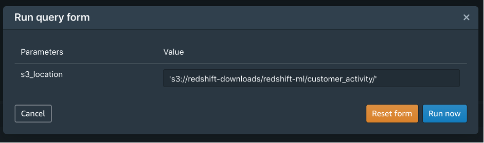
You would probably like to reuse the load query in the future to load data in from another S3 location. In that case, you can use the parameterized query by replacing the S3 URL of the as shown in the following screenshot:

SavingQ2

You can save the query, and then share the query with another user.

When you or other users run the query, a prompt for the parameter will appear as in the following screenshot:

SavingQ3

We discussed how data analysts could load data into their own or the group’s workspace.

We will now discuss using Query Editor V2 to create an external schema to extend your data warehouse to the data lake.

Extending the Data Warehouse to the Data Lake

Extending Data warehouses to Data lakes is part of modern data architecture practices. Amazon Redshift enables this with seamless integration through Data lake running on AWS. Redshift uses Spectrum to allow this extension. You can access data lakes from the Redshift Data warehouse by creating Redshift external schemas.

Query Editor V2 lets you create an external schema referencing an external database in AWS Glue Data Catalogue.

To extend your Data Warehouse to Data Lake, you should have an S3 data lake and AWS Glue Data Catalog database defined for the data lake. Grant permission on AWS Glue to Redshift Cluster Role. You can find more information about external Schema here.

You can navigate to the Create External Schema by using Create Schema wizard, and then selecting the External Schema as shown in the following screenshot:

The Query Editor V2 makes the schema creation experience very easy by hiding the intricacies of the create external schema syntax. You can use the simple interface and provide the required parameters, such as Glue data regions, external database name, and the IAM role. You can browse the Glue Catalog and view the database name.

After you use the create schema option, you can see the schemas in the tree-view. The Query Editor V2 uses distinct icons to distinguish between native Schema and external Schema.

Viewing External Table Definitions

The Query Editor V2 lets data analysts quickly view objects available in external databases and understand their metadata.

You can view tables and columns for a given table by clicking on external Schema and then on a table. When a particular table is selected, its metadata information is displayed in the bottom portion below the tree-view panel. This is a powerful feature, as an analyst can easily understand the data residing externally in the data lake.

You can now run queries against external tables in the external Schema.

In our fictitious enterprise, Marketing Department team members can load data in their own workspace and join the data from their own user/group workspace with the curated data in the enterprise data warehouse or data lake.

Conclusion

This post demonstrated how the Query Editor V2 enabled data analysts to create tables and load data from Amazon S3 easily with a simple wizard.

We also discussed how Query Editor V2 lets you extend the data warehouse to a data lake. The data analysts can easily browse tables in your local data warehouse, data shared from another cluster, or tables in the data lake. You can run queries that can join tables in your data warehouse and data lake. The Query Editor V2 also provides several features for the collaboration of query authoring. You can view the earlier blog to learn more about how the Query Editor V2 simplifies data analysis.

These features let organizations accelerate self-service analytics and end-users deliver the insights faster.

Happy querying!

About the Authors

Bhanu Pittampally is Analytics Specialist Solutions Architect based out of Dallas. He specializes in building analytical solutions. His background is in data warehouse – architecture, development and administration. He is in data and analytical field for over 13 years. His Linkedin profile is here.

Debu Panda is a Principal Product Manager at AWS, is an industry leader in analytics, application platform, and database technologies, and has more than 25 years of experience in the IT world.

Cansu Aksu is a Front End Engineer at AWS, has a several years of experience in developing user interfaces. She is detail oriented, eager to learn and passionate about delivering products and features that solve customer needs and problems

Chengyang Wang is a Frontend Engineer in Redshift Console Team. He worked on a number of new features delivered by redshift in the past 2 years. He thrives to deliver high quality products and aim to improve customer experience from UI

How to Accelerate Building a Lake House Architecture with AWS Glue

2021-08-24 Raghavarao Sodabathina

Post Syndicated from Raghavarao Sodabathina original https://aws.amazon.com/blogs/architecture/how-to-accelerate-building-a-lake-house-architecture-with-aws-glue/

Customers are building databases, data warehouses, and data lake solutions in isolation from each other, each having its own separate data ingestion, storage, management, and governance layers. Often these disjointed efforts to build separate data stores end up creating data silos, data integration complexities, excessive data movement, and data consistency issues. These issues are preventing customers from getting deeper insights. To overcome these issues and easily move data around, a Lake House approach on AWS was introduced.

In this blog post, we illustrate the AWS Glue integration components that you can use to accelerate building a Lake House architecture on AWS. We will also discuss how to derive persona-centric insights from your Lake House using AWS Glue.

Components of the AWS Glue integration system

AWS Glue is a serverless data integration service that facilitates the discovery, preparation, and combination of data. It can be used for analytics, machine learning, and application development. AWS Glue provides all of the capabilities needed for data integration. So you can start analyzing your data and putting it to use in minutes, rather than months.

The following diagram illustrates the various components of the AWS Glue integration system.

Figure 1. AWS Glue integration components

Connect – AWS Glue allows you to connect to various data sources anywhere

Glue connector: AWS Glue provides built-in support for the most commonly used data stores. You can use Amazon Redshift, Amazon RDS, Amazon Aurora, Microsoft SQL Server, MySQL, MongoDB, or PostgreSQL using JDBC connections. AWS Glue also allows you to use custom JDBC drivers in your extract, transform, and load (ETL) jobs. For data stores that are not natively supported such as SaaS applications, you can use connectors. You can also subscribe to several connectors offered in the AWS Marketplace.

Glue crawlers: You can use a crawler to populate the AWS Glue Data Catalog with tables. A crawler can crawl multiple data stores in a single pass. Upon completion, the crawler creates or updates one or more tables in your Data Catalog. Extract, transform, and load (ETL) jobs that you define in AWS Glue use these Data Catalog tables as sources and targets.

Catalog – AWS Glue simplifies data discovery and governance

Glue Data Catalog: The Data Catalog serves as the central metadata catalog for the entire data landscape.

Glue Schema Registry: The AWS Glue Schema Registry allows you to centrally discover, control, and evolve data stream schemas. With AWS Glue Schema Registry, you can manage and enforce schemas on your data streaming applications.

Data quality – AWS Glue helps you author and monitor data quality rules

Glue DataBrew: AWS Glue DataBrew allows data scientists and data analysts to clean and normalize data. You can use a visual interface, reducing the time it takes to prepare data by up to 80%. With Glue DataBrew, you can visualize, clean, and normalize data directly from your data lake, data warehouses, and databases.

Curate data: You can use either Glue development endpoint or AWS Glue Studio to curate your data.

AWS Glue development endpoint is an environment that you can use to develop and test your AWS Glue scripts. You can choose either Amazon SageMaker notebook or Apache Zeppelin notebook as an environment.

AWS Glue Studio is a new visual interface for AWS Glue that supports extract-transform-and-load (ETL) developers. You can author, run, and monitor AWS Glue ETL jobs. You can now use a visual interface to compose jobs that move and transform data, and run them on AWS Glue.

AWS Data Exchange makes it easy for AWS customers to securely exchange and use third-party data in AWS. This is for data providers who want to structure their data across multiple datasets or enrich their products with additional data. You can publish additional datasets to your products using the AWS Data Exchange.

Deequ is an open-source data quality library developed internally at Amazon, for data quality. It provides multiple features such as automatic constraint suggestions and verification, metrics computation, and data profiling.

Build a Lake House architecture faster, using AWS Glue

Figure 2 illustrates how you can build a Lake House using AWS Glue components.

Figure 2. Building Lake House architectures with AWS Glue

The architecture flow follows these general steps:

Glue crawlers scan the data from various data sources and populate the Data Catalog for your Lake House.
The Data Catalog serves as the central metadata catalog for the entire data landscape.
Once data is cataloged, fine-grained access control is applied to the tables through AWS Lake Formation.
Curate your data with business and data quality rules by using Glue Studio, Glue development endpoints, or Glue DataBrew. Place transformed data in a curated Amazon S3 for purpose built analytics downstream.
Facilitate data movement with AWS Glue to and from your data lake, databases, and data warehouse by using Glue connections. Use AWS Glue Elastic views to replicate the data across the Lake House.

Derive persona-centric insights from your Lake House using AWS Glue

Many organizations want to gather observations from increasingly larger volumes of acquired data. These insights help them make data-driven decisions with speed and agility. They must use a central data lake, a ring of purpose-built data services, and data warehouses based on persona or job function.

Figure 3 illustrates the Lake House inside-out data movement with AWS Glue DataBrew, Amazon Athena, Amazon Redshift, and Amazon QuickSight to perform persona-centric data analytics.

Figure 3. Lake House persona-centric data analytics using AWS Glue

This shows how Lake House components serve various personas in an organization:

Data ingestion: Data is ingested to Amazon Simple Storage Service (S3) from different sources.
Data processing: Data curators and data scientists use DataBrew to validate, clean, and enrich the data. Amazon Athena is also used to run improvised queries to analyze the data in the lake. The transformation is shared with data engineers to set up batch processing.
Batch data processing: Data engineers or developers set up batch jobs in AWS Glue and AWS Glue DataBrew. Jobs can be initiated by an event, or can be scheduled to run periodically.
Data analytics: Data/Business analysts can now analyze prepared dataset in Amazon Redshift or in Amazon S3 using Athena.
Data visualizations: Business analysts can create visuals in QuickSight. Data curators can enrich data from multiple sources. Admins can enforce security and data governance. Developers can embed QuickSight dashboard in applications.

Conclusion

Using a Lake House architecture will help you get persona-centric insights quickly from all of your data based on user role or job function. In this blog post, we describe several AWS Glue components and AWS purpose-built services that you can use to build Lake House architectures on AWS. We have also presented persona-centric Lake House analytics architecture using AWS Glue, to help you derive insights from your Lake House.

Read more and get started on building Lake House Architectures on AWS.

What is a Lake House approach?
Harness the power of your data with AWS Analytics
AWS Lake House reference architecture (scroll down in blog)
Derive Insights from AWS Lake House whitepaper
AWS Glue Developer Guide

How MEDHOST’s cardiac risk prediction successfully leveraged AWS analytic services

2021-08-23 Pandian Velayutham

Post Syndicated from Pandian Velayutham original https://aws.amazon.com/blogs/big-data/how-medhosts-cardiac-risk-prediction-successfully-leveraged-aws-analytic-services/

MEDHOST has been providing products and services to healthcare facilities of all types and sizes for over 35 years. Today, more than 1,000 healthcare facilities are partnering with MEDHOST and enhancing their patient care and operational excellence with its integrated clinical and financial EHR solutions. MEDHOST also offers a comprehensive Emergency Department Information System with business and reporting tools. Since 2013, MEDHOST’s cloud solutions have been utilizing Amazon Web Services (AWS) infrastructure, data source, and computing power to solve complex healthcare business cases.

MEDHOST can utilize the data available in the cloud to provide value-added solutions for hospitals solving complex problems, like predicting sepsis, cardiac risk, and length of stay (LOS) as well as reducing re-admission rates. This requires a solid foundation of data lake and elastic data pipeline to keep up with multi-terabyte data from thousands of hospitals. MEDHOST has invested a significant amount of time evaluating numerous vendors to determine the best solution for its data needs. Ultimately, MEDHOST designed and implemented machine learning/artificial intelligence capabilities by leveraging AWS Data Lab and an end-to-end data lake platform that enables a variety of use cases such as data warehousing for analytics and reporting.

Since you’re reading this post, you may also be interested in the following:

MEDHOST expands multi-tenant cloud EHR capabilities with AWS (AWS for Industries)

Getting started

MEDHOST’s initial objectives in evaluating vendors were to:

Build a low-cost data lake solution to provide cardiac risk prediction for patients based on health records
Provide an analytical solution for hospital staff to improve operational efficiency
Implement a proof of concept to extend to other machine learning/artificial intelligence solutions

The AWS team proposed AWS Data Lab to architect, develop, and test a solution to meet these objectives. The collaborative relationship between AWS and MEDHOST, AWS’s continuous innovation, excellent support, and technical solution architects helped MEDHOST select AWS over other vendors and products. AWS Data Lab’s well-structured engagement helped MEDHOST define clear, measurable success criteria that drove the implementation of the cardiac risk prediction and analytical solution platform. The MEDHOST team consisted of architects, builders, and subject matter experts (SMEs). By connecting MEDHOST experts directly to AWS technical experts, the MEDHOST team gained a quick understanding of industry best practices and available services allowing MEDHOST team to achieve most of the success criteria at the end of a four-day design session. MEDHOST is now in the process of moving this work from its lower to upper environment to make the solution available for its customers.

Solution

For this solution, MEDHOST and AWS built a layered pipeline consisting of ingestion, processing, storage, analytics, machine learning, and reinforcement components. The following diagram illustrates the Proof of Concept (POC) that was implemented during the four-day AWS Data Lab engagement.

Ingestion layer

The ingestion layer is responsible for moving data from hospital production databases to the landing zone of the pipeline.

The hospital data was stored in an Amazon RDS for PostgreSQL instance and moved to the landing zone of the data lake using AWS Database Migration Service (DMS). DMS made migrating databases to the cloud simple and secure. Using its ongoing replication feature, MEDHOST and AWS implemented change data capture (CDC) quickly and efficiently so MEDHOST team could spend more time focusing on the most interesting parts of the pipeline.

Processing layer

The processing layer was responsible for performing extract, tranform, load (ETL) on the data to curate them for subsequent uses.

MEDHOST used AWS Glue within its data pipeline for crawling its data layers and performing ETL tasks. The hospital data copied from RDS to Amazon S3 was cleaned, curated, enriched, denormalized, and stored in parquet format to act as the heart of the MEDHOST data lake and a single source of truth to serve any further data needs. During the four-day Data Lab, MEDHOST and AWS targeted two needs: powering MEDHOST’s data warehouse used for analytics and feeding training data to the machine learning prediction model. Even though there were multiple challenges, data curation is a critical task which requires an SME. AWS Glue’s serverless nature, along with the SME’s support during the Data Lab, made developing the required transformations cost efficient and uncomplicated. Scaling and cluster management was addressed by the service, which allowed the developers to focus on cleaning data coming from homogenous hospital sources and translating the business logic to code.

Storage layer

The storage layer provided low-cost, secure, and efficient storage infrastructure.

MEDHOST used Amazon S3 as a core component of its data lake. AWS DMS migration tasks saved data to S3 in .CSV format. Crawling data with AWS Glue made this landing zone data queryable and available for further processing. The initial AWS Glue ETL job stored the parquet formatted data to the data lake and its curated zone bucket. MEDHOST also used S3 to store the .CSV formatted data set that will be used to train, test, and validate its machine learning prediction model.

Analytics layer

The analytics layer gave MEDHOST pipeline reporting and dashboarding capabilities.

The data was in parquet format and partitioned in the curation zone bucket populated by the processing layer. This made querying with Amazon Athena or Amazon Redshift Spectrum fast and cost efficient.

From the Amazon Redshift cluster, MEDHOST created external tables that were used as staging tables for MEDHOST data warehouse and implemented an UPSERT logic to merge new data in its production tables. To showcase the reporting potential that was unlocked by the MEDHOST analytics layer, a connection was made to the Redshift cluster to Amazon QuickSight. Within minutes MEDHOST was able to create interactive analytics dashboards with filtering and drill-down capabilities such as a chart that showed the number of confirmed disease cases per US state.

Machine learning layer

The machine learning layer used MEDHOST’s existing data sets to train its cardiac risk prediction model and make it accessible via an endpoint.

Before getting into Data Lab, the MEDHOST team was not intimately familiar with machine learning. AWS Data Lab architects helped MEDHOST quickly understand concepts of machine learning and select a model appropriate for its use case. MEDHOST selected XGBoost as its model since cardiac prediction falls within regression technique. MEDHOST’s well architected data lake enabled it to quickly generate training, testing, and validation data sets using AWS Glue.

Amazon SageMaker abstracted underlying complexity of setting infrastructure for machine learning. With few clicks, MEDHOST started Jupyter notebook and coded the components leading to fitting and deploying its machine learning prediction model. Finally, MEDHOST created the endpoint for the model and ran REST calls to validate the endpoint and trained model. As a result, MEDHOST achieved the goal of predicting cardiac risk. Additionally, with Amazon QuickSight’s SageMaker integration, AWS made it easy to use SageMaker models directly in visualizations. QuickSight can call the model’s endpoint, send the input data to it, and put the inference results into the existing QuickSight data sets. This capability made it easy to display the results of the models directly in the dashboards. Read more about QuickSight’s SageMaker integration here.

Reinforcement layer

Finally, the reinforcement layer guaranteed that the results of the MEDHOST model were captured and processed to improve performance of the model.

The MEDHOST team went beyond the original goal and created an inference microservice to interact with the endpoint for prediction, enabled abstracting of the machine learning endpoint with the well-defined domain REST endpoint, and added a standard security layer to the MEDHOST application.

When there is a real-time call from the facility, the inference microservice gets inference from the SageMaker endpoint. Records containing input and inference data are fed to the data pipeline again. MEDHOST used Amazon Kinesis Data Streams to push records in real time. However, since retraining the machine learning model does not need to happen in real time, the Amazon Kinesis Data Firehose enabled MEDHOST to micro-batch records and efficiently save them to the landing zone bucket so that the data could be reprocessed.

Conclusion

Collaborating with AWS Data Lab enabled MEDHOST to:

Store single source of truth with low-cost storage solution (data lake)
Complete data pipeline for a low-cost data analytics solution
Create an almost production-ready code for cardiac risk prediction

The MEDHOST team learned many concepts related to data analytics and machine learning within four days. AWS Data Lab truly helped MEDHOST deliver results in an accelerated manner.

About the Authors

Pandian Velayutham is the Director of Engineering at MEDHOST. His team is responsible for delivering cloud solutions, integration and interoperability, and business analytics solutions. MEDHOST utilizes modern technology stack to provide innovative solutions to our customers. Pandian Velayutham is a technology evangelist and public cloud technology speaker.

George Komninos is a Data Lab Solutions Architect at AWS. He helps customers convert their ideas to a production-ready data product. Before AWS, he spent 3 years at Alexa Information domain as a data engineer. Outside of work, George is a football fan and supports the greatest team in the world, Olympiacos Piraeus.

Deploy data lake ETL jobs using CDK Pipelines

2021-07-30 Ravi Itha

Post Syndicated from Ravi Itha original https://aws.amazon.com/blogs/devops/deploying-data-lake-etl-jobs-using-cdk-pipelines/

Many organizations are building data lakes on AWS, which provides the most secure, scalable, comprehensive, and cost-effective portfolio of services. Like any application development project, a data lake must answer a fundamental question: “What is the DevOps strategy?” Defining a DevOps strategy for a data lake requires extensive planning and multiple teams. This typically requires multiple development and test cycles before maturing enough to support a data lake in a production environment. If an organization doesn’t have the right people, resources, and processes in place, this can quickly become daunting.

What if your data engineering team uses basic building blocks to encapsulate data lake infrastructure and data processing jobs? This is where CDK Pipelines brings the full benefit of infrastructure as code (IaC). CDK Pipelines is a high-level construct library within the AWS Cloud Development Kit (AWS CDK) that makes it easy to set up a continuous deployment pipeline for your AWS CDK applications. The AWS CDK provides essential automation for your release pipelines so that your development and operations team remain agile and focus on developing and delivering applications on the data lake.

In this post, we discuss a centralized deployment solution utilizing CDK Pipelines for data lakes. This implements a DevOps-driven data lake that delivers benefits such as continuous delivery of data lake infrastructure, data processing, and analytical jobs through a configuration-driven multi-account deployment strategy. Let’s dive in!

Data lakes on AWS

A data lake is a centralized repository where you can store all of your structured and unstructured data at any scale. Store your data as is, without having to first structure it, and run different types of analytics—from dashboards and visualizations to big data processing, real-time analytics, and machine learning in order to guide better decisions. To further explore data lakes, refer to What is a data lake?

We design a data lake with the following elements:

Secure data storage
Data cataloging in a central repository
Data movement
Data analysis

The following figure represents our data lake.

Data Lake on AWS

We use three Amazon Simple Storage Service (Amazon S3) buckets:

raw – Stores the input data in its original format
conformed – Stores the data that meets the data lake quality requirements
purpose-built – Stores the data that is ready for consumption by applications or data lake consumers

The data lake has a producer where we ingest data into the raw bucket at periodic intervals. We utilize the following tools: AWS Glue processes and analyzes the data. AWS Glue Data Catalog persists metadata in a central repository. AWS Lambda and AWS Step Functions schedule and orchestrate AWS Glue extract, transform, and load (ETL) jobs. Amazon Athena is used for interactive queries and analysis. Finally, we engage various AWS services for logging, monitoring, security, authentication, authorization, alerting, and notification.

A common data lake practice is to have multiple environments such as dev, test, and production. Applying the IaC principle for data lakes brings the benefit of consistent and repeatable runs across multiple environments, self-documenting infrastructure, and greater flexibility with resource management. The AWS CDK offers high-level constructs for use with all of our data lake resources. This simplifies usage and streamlines implementation.

Before exploring the implementation, let’s gain further scope of how we utilize our data lake.

The solution

Our goal is to implement a CI/CD solution that automates the provisioning of data lake infrastructure resources and deploys ETL jobs interactively. We accomplish this as follows: 1) applying separation of concerns (SoC) design principle to data lake infrastructure and ETL jobs via dedicated source code repositories, 2) a centralized deployment model utilizing CDK pipelines, and 3) AWS CDK enabled ETL pipelines from the start.

Data lake infrastructure

Our data lake infrastructure provisioning includes Amazon S3 buckets, S3 bucket policies, AWS Key Management Service (KMS) encryption keys, Amazon Virtual Private Cloud (Amazon VPC), subnets, route tables, security groups, VPC endpoints, and secrets in AWS Secrets Manager. The following diagram illustrates this.

Data Lake Infrastructure

Data lake ETL jobs

For our ETL jobs, we process New York City TLC Trip Record Data. The following figure displays our ETL process, wherein we run two ETL jobs within a Step Functions state machine.

AWS Glue ETL Jobs

Here are a few important details:

A file server uploads files to the S3 raw bucket of the data lake. The file server is a data producer and source for the data lake. We assume that the data is pushed to the raw bucket.
Amazon S3 triggers an event notification to the Lambda function.
The function inserts an item in the Amazon DynamoDB table in order to track the file processing state. The first state written indicates the AWS Step Function start.
The function starts the state machine.
The state machine runs an AWS Glue job (Apache Spark).
The job processes input data from the raw zone to the data lake conformed zone. The job also converts CSV input data to Parquet formatted data.
The job updates the Data Catalog table with the metadata of the conformed Parquet file.
A second AWS Glue job (Apache Spark) processes the input data from the conformed zone to the purpose-built zone of the data lake.
The job fetches ETL transformation rules from the Amazon S3 code bucket and transforms the input data.
The job stores the result in Parquet format in the purpose-built zone.
The job updates the Data Catalog table with the metadata of the purpose-built Parquet file.
The job updates the DynamoDB table and updates the job status to completed.
An Amazon Simple Notification Service (Amazon SNS) notification is sent to subscribers that states the job is complete.
Data engineers or analysts can now analyze data via Athena.

We will discuss data formats, Glue jobs, ETL transformation logics, data cataloging, auditing, notification, orchestration, and data analysis in more detail in AWS CDK Pipelines for Data Lake ETL Deployment GitHub repository. This will be discussed in the subsequent section.

Centralized deployment

Now that we have data lake infrastructure and ETL jobs ready, let’s define our deployment model. This model is based on the following design principles:

A dedicated AWS account to run CDK pipelines.
One or more AWS accounts into which the data lake is deployed.
The data lake infrastructure has a dedicated source code repository. Typically, data lake infrastructure is a one-time deployment and rarely evolves. Therefore, a dedicated code repository provides a landing zone for your data lake.
Each ETL job has a dedicated source code repository. Each ETL job may have unique AWS service, orchestration, and configuration requirements. Therefore, a dedicated source code repository will help you more flexibly build, deploy, and maintain ETL jobs.

We organize our source code repo into three branches: dev (main), test, and prod. In the deployment account, we manage three separate CDK Pipelines and each pipeline is sourced from a dedicated branch. Here we choose a branch-based software development method in order to demonstrate the strategy in more complex scenarios where integration testing and validation layers require human intervention. As well, these may not immediately follow with a corresponding release or deployment due to their manual nature. This facilitates the propagation of changes through environments without blocking independent development priorities. We accomplish this by isolating resources across environments in the central deployment account, allowing for the independent management of each environment, and avoiding cross-contamination during each pipeline’s self-mutating updates. The following diagram illustrates this method.

Centralized deployment

Note: This centralized deployment strategy can be adopted for trunk-based software development with minimal solution modification.

Deploying data lake ETL jobs

The following figure illustrates how we utilize CDK Pipelines to deploy data lake infrastructure and ETL jobs from a central deployment account. This model follows standard nomenclature from the AWS CDK. Each repository represents a cloud infrastructure code definition. This includes the pipelines construct definition. Pipelines have one or more actions, such as cloning the source code (source action) and synthesizing the stack into an AWS CloudFormation template (synth action). Each pipeline has one or more stages, such as testing and deploying. In an AWS CDK app context, the pipelines construct is a stack like any other stack. Therefore, when the AWS CDK app is deployed, a new pipeline is created in AWS CodePipeline.

This provides incredible flexibility regarding DevOps. In other words, as a developer with an understanding of AWS CDK APIs, you can harness the power and scalability of AWS services such as CodePipeline, AWS CodeBuild, and AWS CloudFormation.

Deploying data lake ETL jobs using CDK Pipelines

Here are a few important details:

The DevOps administrator checks in the code to the repository.
The DevOps administrator (with elevated access) facilitates a one-time manual deployment on a target environment. Elevated access includes administrative privileges on the central deployment account and target AWS environments.
CodePipeline periodically listens to commit events on the source code repositories. This is the self-mutating nature of CodePipeline. It’s configured to work with and can update itself according to the provided definition.
Code changes made to the main repo branch are automatically deployed to the data lake dev environment.
Code changes to the repo test branch are automatically deployed to the test environment.
Code changes to the repo prod branch are automatically deployed to the prod environment.

CDK Pipelines starter kits for data lakes

Want to get going quickly with CDK Pipelines for your data lake? Start by cloning our two GitHub repositories. Here is a summary:

AWS CDK Pipelines for Data Lake Infrastructure Deployment

This repository contains the following reusable resources:

CDK Application
CDK Pipelines stack
CDK Pipelines deploy stage
Amazon VPC stack
Amazon S3 stack

It also contains the following automation scripts:

AWS environments configuration
Deployment account bootstrapping
Target account bootstrapping
Account secrets configuration (e.g., GitHub access tokens)

AWS CDK Pipelines for Data Lake ETL Deployment

This repository contains the following reusable resources:

CDK Application
CDK Pipelines stack
CDK Pipelines deploy stage
Amazon DynamoDB stack
AWS Glue stack
AWS Step Functions stack

It also contains the following:

AWS Lambda scripts
AWS Glue scripts
AWS Step Functions State machine script

Advantages

This section summarizes some of the advantages offered by this solution.

Scalable and centralized deployment model

We utilize a scalable and centralized deployment model to deliver end-to-end automation. This allows DevOps and data engineers to use the single responsibility principal while maintaining precise control over the deployment strategy and code quality. The model can readily be expanded to more accounts, and the pipelines are responsive to custom controls within each environment, such as a production approval layer.

Configuration-driven deployment

Configuration in the source code and AWS Secrets Manager allow deployments to utilize targeted values that are declared globally in a single location. This provides consistent management of global configurations and dependencies such as resource names, AWS account Ids, Regions, and VPC CIDR ranges. Similarly, the CDK Pipelines export outputs from CloudFormation stacks for later consumption via other resources.

Repeatable and consistent deployment of new ETL jobs

Continuous integration and continuous delivery (CI/CD) pipelines allow teams to deploy to production more frequently. Code changes can be safely and securely propagated through environments and released for deployment. This allows rapid iteration on data processing jobs, and these jobs can be changed in isolation from pipeline changes, resulting in reliable workflows.

Cleaning up

You may delete the resources provisioned by utilizing the starter kits. You can do this by running the cdk destroy command using AWS CDK Toolkit. For detailed instructions, refer to the Clean up sections in the starter kit README files.

Conclusion

In this post, we showed how to utilize CDK Pipelines to deploy infrastructure and data processing ETL jobs of your data lake in dev, test, and production AWS environments. We provided two GitHub repositories for you to test and realize the full benefits of this solution first hand. We encourage you to fork the repositories, bring your ETL scripts, bootstrap your accounts, configure account parameters, and continuously delivery your data lake ETL jobs.

Let’s stay in touch via the GitHub—AWS CDK Pipelines for Data Lake Infrastructure Deployment and AWS CDK Pipelines for Data Lake ETL Deployment.

About the authors

Ravi Itha

Ravi Itha is a Sr. Data Architect at AWS. He works with customers to design and implement Data Lakes, Analytics, and Microservices on AWS. He is an open-source committer and has published more than a dozen solutions using AWS CDK, AWS Glue, AWS Lambda, AWS Step Functions, Amazon ECS, Amazon MQ, Amazon SQS, Amazon Kinesis Data Streams, and Amazon Kinesis Data Analytics for Apache Flink. His solutions can be found at his GitHub handle. Outside of work, he is passionate about books, cooking, movies, and yoga.

Isaiah Grant

Isaiah Grant is a Cloud Consultant at 2nd Watch. His primary function is to design architectures and build cloud-based applications and services. He leads customer engagements and helps customers with enterprise cloud adoptions. In his free time, he is engaged in local community initiatives and enjoys being outdoors with his family.

Zahid Ali

Zahid Ali is a Data Architect at AWS. He helps customers design, develop, and implement data warehouse and Data Lake solutions on AWS. Outside of work he enjoys playing tennis, spending time outdoors, and traveling.

Amazon MSK backup for Archival, Replay, or Analytics

2021-02-19 Rohit Yadav

Post Syndicated from Rohit Yadav original https://aws.amazon.com/blogs/architecture/amazon-msk-backup-for-archival-replay-or-analytics/

Amazon MSK is a fully managed service that helps you build and run applications that use Apache Kafka to process streaming data. Apache Kafka is an open-source platform for building real-time streaming data pipelines and applications. With Amazon MSK, you can use native Apache Kafka APIs to populate data lakes. You can also stream changes to and from databases, and power machine learning and analytics applications.

Amazon MSK simplifies the setup, scaling, and management of clusters running Apache Kafka. MSK manages the provisioning, configuration, and maintenance of resources for a highly available Kafka clusters. It is fully compatible with Apache Kafka and supports familiar community-build tools such as MirrorMaker 2.0, Kafka Connect and Kafka streams.

Introduction

In the past few years, the volume of data that companies must ingest has increased significantly. Information comes from various sources, like transactional databases, system logs, SaaS platforms, mobile, and IoT devices. Businesses want to act as soon as the data arrives. This has resulted in increased adoption of scalable real-time streaming solutions. These solutions scale horizontally to provide the needed throughput to process data in real time, with milliseconds of latency. Customers have adopted Amazon MSK as a top choice of streaming platforms. Amazon MSK gives you the flexibility to retain topic data for longer term (default 7 days). This supports replay, analytics, and machine learning based use cases. When IT and business systems are producing and processing terabytes of data per hour, it can become expensive to store, manage, and retrieve data. This has led to legacy data archival processes moving towards cheaper, reliable, and long-term storage solutions like Amazon Simple Storage Service (S3).

Following are some of the benefits of archiving Amazon MSK topic data to Amazon S3:

Reduced Cost – You only must retain the data in the cluster based on your Recovery Point Objective (RPO). Any historical data can be archived in Amazon S3 and replayed if necessary.
Integration with Enterprise Data Lake – Since your data is available in S3, you can now integrate with other data analytics services like Amazon EMR, AWS Glue, Amazon Athena, to run data aggregation and analytics. For example, you can build reports to visualize month over month changes.
Optimize Machine Learning Workloads – Machine learning applications will be able to train new models and improve predictions using historical streams of data available in Amazon S3. This also enables better integration with Amazon Machine Learning services.
Compliance – Long-term data archival for regulatory and security compliance.
Backloading data to other systems – Ability to rebuild data into other application environments such as pre-prod, testing, and more.

There are many benefits to using Amazon S3 as long-term storage for Amazon MSK topics. Let’s dive deeper into the recommended architecture for this pattern. We will present an architecture to back up Amazon MSK topics to Amazon S3 in real time. In addition, we’ll demonstrate some of the use cases previously mentioned.

Architecture

The diagram following illustrates the architecture for building a real-time archival pipeline to archive Amazon MSK topics to S3. This architecture uses an AWS Lambda function to process records from your Amazon MSK cluster when the cluster is configured as an event source. As a consumer, you don’t need to worry about infrastructure management or scaling with Lambda. You only pay for what you consume, so you don’t pay for over-provisioned infrastructure.

To create an event source mapping, you can add your Amazon MSK cluster in a Lambda function trigger. The Lambda service internally polls for new records or messages from the event source, and then synchronously invokes the target Lambda function. Lambda reads the messages in batches from one or more partitions and provides these to your function as an event payload. The function then processes records, and sends the payload to an Amazon Kinesis Data Firehose delivery stream. We use Kinesis Data Firehose delivery stream because it can natively batch, compress, transform, and encrypt your events before loading to S3.

In this architecture, Kinesis Data Firehose delivers the records received from Lambda in Gzip file to Amazon S3. These files are partitioned in hive style format by Kinesis Data Firehose:

data/year = yyyy/month = MM/day = dd/hour = HH

Figure 1. Archival Architecture

Let’s review some of the possible solutions that can be built on this archived data.

Integration with Enterprise Data Lake

The architecture diagram following shows how you can integrate the archived data in Amazon S3 with your Enterprise Data Lake. Since the data files are prefixed in hive style format, you can partition and store the Data Catalog in AWS Glue. With partitioning in place, you can perform optimizations like partition pruning, which enables predicate pushdown for improved performance of your analytics queries. You can also use AWS Data Analytics services like Amazon EMR and AWS Glue for batch analytics. Amazon Athena can be used to run serverless SQL-like interactive queries on visualization and data.

Data currently gets stored in JSON files. Following are some of the services/tools that can be integrated with your archive for reporting, analytics, visualization, and machine learning requirements.

Figure 2. Analytics Architecture

Cloning data into other application environments

There are use cases where you would want to use this data to clone other application environments using this archive.

These clusters could be used for testing or debugging purposes. You could decide to use only a subset of your data from the archive. Let’s say you want to debug an issue beyond the configured retention period, but not replicate all the data to your testing environment. With archived data in S3, you can build downstream jobs to filter data that can be loaded into a new Amazon MSK cluster. The following diagram highlights this pattern:

Figure 3. Replay Architecture

Ready for a Test Drive

To help you get started, we would like to introduce an AWS Solution: AWS Streaming Data Solution for Amazon MSK (scroll down and see Option 3 tab). There is a single-click AWS CloudFormation template, which can assist you in quickly provisioning resources. This will get your real-time archival pipeline for Amazon MSK up and running quickly. This solution shortens your development time by removing or reducing the need for you to:

Model and provision resources using AWS CloudFormation
Set up Amazon CloudWatch alarms, dashboards, and logging
Manually implement streaming data best practices in AWS

This solution is data and logic agnostic, enabling you to start with boilerplate code and start customizing quickly. After deployment, use this solution’s monitoring capabilities to transition easily to production.

Conclusion

In this post, we explained the architecture to build a scalable, highly available real-time archival of Amazon MSK topics to long term storage in Amazon S3. The architecture was built using Amazon MSK, AWS Lambda, Amazon Kinesis Data Firehose, and Amazon S3. The architecture also illustrates how you can integrate your Amazon MSK streaming data in S3 with your Enterprise Data Lake.

Use Macie to discover sensitive data as part of automated data pipelines

2020-12-09 Brandon Wu

Post Syndicated from Brandon Wu original https://aws.amazon.com/blogs/security/use-macie-to-discover-sensitive-data-as-part-of-automated-data-pipelines/

Data is a crucial part of every business and is used for strategic decision making at all levels of an organization. To extract value from their data more quickly, Amazon Web Services (AWS) customers are building automated data pipelines—from data ingestion to transformation and analytics. As part of this process, my customers often ask how to prevent sensitive data, such as personally identifiable information, from being ingested into data lakes when it’s not needed. They highlight that this challenge is compounded when ingesting unstructured data—such as files from process reporting, text files from chat transcripts, and emails. They also mention that identifying sensitive data inadvertently stored in structured data fields—such as in a comment field stored in a database—is also a challenge.

In this post, I show you how to integrate Amazon Macie as part of the data ingestion step in your data pipeline. This solution provides an additional checkpoint that sensitive data has been appropriately redacted or tokenized prior to ingestion. Macie is a fully managed data security and privacy service that uses machine learning and pattern matching to discover sensitive data in AWS.

When Macie discovers sensitive data, the solution notifies an administrator to review the data and decide whether to allow the data pipeline to continue ingesting the objects. If allowed, the objects will be tagged with an Amazon Simple Storage Service (Amazon S3) object tag to identify that sensitive data was found in the object before progressing to the next stage of the pipeline.

This combination of automation and manual review helps reduce the risk that sensitive data—such as personally identifiable information—will be ingested into a data lake. This solution can be extended to fit your use case and workflows. For example, you can define custom data identifiers as part of your scans, add additional validation steps, create Macie suppression rules to archive findings automatically, or only request manual approvals for findings that meet certain criteria (such as high severity findings).

Solution overview

Many of my customers are building serverless data lakes with Amazon S3 as the primary data store. Their data pipelines commonly use different S3 buckets at each stage of the pipeline. I refer to the S3 bucket for the first stage of ingestion as the raw data bucket. A typical pipeline might have separate buckets for raw, curated, and processed data representing different stages as part of their data analytics pipeline.

Typically, customers will perform validation and clean their data before moving it to a raw data zone. This solution adds validation steps to that pipeline after preliminary quality checks and data cleaning is performed, noted in blue (in layer 3) of Figure 1. The layers outlined in the pipeline are:

Ingestion – Brings data into the data lake.
Storage – Provides durable, scalable, and secure components to store the data—typically using S3 buckets.
Processing – Transforms data into a consumable state through data validation, cleanup, normalization, transformation, and enrichment. This processing layer is where the additional validation steps are added to identify instances of sensitive data that haven’t been appropriately redacted or tokenized prior to consumption.
Consumption – Provides tools to gain insights from the data in the data lake.

Figure 1: Data pipeline with sensitive data scan

The application runs on a scheduled basis (four times a day, every 6 hours by default) to process data that is added to the raw data S3 bucket. You can customize the application to perform a sensitive data discovery scan during any stage of the pipeline. Because most customers do their extract, transform, and load (ETL) daily, the application scans for sensitive data on a scheduled basis before any crawler jobs run to catalog the data and after typical validation and data redaction or tokenization processes complete.

You can expect that this additional validation will add 5–10 minutes to your pipeline execution at a minimum. The validation processing time will scale linearly based on object size, but there is a start-up time per job that is constant.

If sensitive data is found in the objects, an email is sent to the designated administrator requesting an approval decision, which they indicate by selecting the link corresponding to their decision to approve or deny the next step. In most cases, the reviewer will choose to adjust the sensitive data cleanup processes to remove the sensitive data, deny the progression of the files, and re-ingest the files in the pipeline.

Additional considerations for deploying this application for regular use are discussed at the end of the blog post.

Application components

The following resources are created as part of the application:

Identity and Access Management (IAM) managed policies grant the necessary permissions for the AWS Lambda functions to access AWS resources that are part of the application.
S3 buckets store data in various stages of processing: A raw data bucket for uploading objects for the data pipeline, a scanning bucket where objects are scanned for sensitive data, a manual review bucket holding objects where sensitive data was discovered, and a scanned data bucket for starting the next ingestion step of the data pipeline.
Lambda functions execute the logic to run the sensitive data scans and workflow.
AWS Step Functions Standard Workflows orchestrate the Lambda functions for the business logic.
Amazon Macie sensitive data discovery jobs scan the scanning stage S3 bucket for sensitive data.
An Amazon EventBridge rule starts the Step Functions workflow execution on a recurring schedule.
An Amazon Simple Notification Service (Amazon SNS) topic sends notifications to review sensitive data discovered in the pipeline.
An Amazon API Gateway REST API with two resources receives the decisions of the sensitive data reviewer as part of a manual workflow.

Note: the application uses various AWS services, and there are costs associated with these resources after the Free Tier usage. See AWS Pricing for details. The primary drivers of the solution cost will be the amount of data ingested through the pipeline, both for Amazon S3 storage and data processed for sensitive data discovery with Macie.

The architecture of the application is shown in Figure 2 and described in the text that follows.

Figure 2: Application architecture and logic

Application logic

Objects are uploaded to the raw data S3 bucket as part of the data ingestion process.
A scheduled EventBridge rule runs the sensitive data scan Step Functions workflow.
triggerMacieScan Lambda function moves objects from the raw data S3 bucket to the scan stage S3 bucket.
triggerMacieScan Lambda function creates a Macie sensitive data discovery job on the scan stage S3 bucket.
checkMacieStatus Lambda function checks the status of the Macie sensitive data discovery job.
isMacieStatusCompleteChoice Step Functions Choice state checks whether the Macie sensitive data discovery job is complete.
1. If yes, the getMacieFindingsCount Lambda function runs.
2. If no, the Step Functions Wait state waits 60 seconds and then restarts Step 5.
getMacieFindingsCount Lambda function counts all of the findings from the Macie sensitive data discovery job.
isSensitiveDataFound Step Functions Choice state checks whether sensitive data was found in the Macie sensitive data discovery job.
1. If there was sensitive data discovered, run the triggerManualApproval Lambda function.
2. If there was no sensitive data discovered, run the moveAllScanStageS3Files Lambda function.
moveAllScanStageS3Files Lambda function moves all of the objects from the scan stage S3 bucket to the scanned data S3 bucket.
triggerManualApproval Lambda function tags and moves objects with sensitive data discovered to the manual review S3 bucket, and moves objects with no sensitive data discovered to the scanned data S3 bucket. The function then sends a notification to the ApprovalRequestNotification Amazon SNS topic as a notification that manual review is required.
Email is sent to the email address that’s subscribed to the ApprovalRequestNotification Amazon SNS topic (from the application deployment template) for the manual review user with the option to Approve or Deny pipeline ingestion for these objects.
Manual review user assesses the objects with sensitive data in the manual review S3 bucket and selects the Approve or Deny links in the email.
The decision request is sent from the Amazon API Gateway to the receiveApprovalDecision Lambda function.
manualApprovalChoice Step Functions Choice state checks the decision from the manual review user.
1. If denied, run the deleteManualReviewS3Files Lambda function.
2. If approved, run the moveToScannedDataS3Files Lambda function.
deleteManualReviewS3Files Lambda function deletes the objects from the manual review S3 bucket.
moveToScannedDataS3Files Lambda function moves the objects from the manual review S3 bucket to the scanned data S3 bucket.
The next step of the automated data pipeline will begin with the objects in the scanned data S3 bucket.

Prerequisites

For this application, you need the following prerequisites:

The AWS Command Line Interface (AWS CLI) installed and configured for use.
The AWS Serverless Application Model (AWS SAM) CLI installed and configured for use.
An IAM role or user with permissions to publish serverless applications using the AWS SAM CLI.

You can use AWS Cloud9 to deploy the application. AWS Cloud9 includes the AWS CLI and AWS SAM CLI to simplify setting up your development environment.

Deploy the application with AWS SAM CLI

You can deploy this application using the AWS SAM CLI. AWS SAM uses AWS CloudFormation as the underlying deployment mechanism. AWS SAM is an open-source framework that you can use to build serverless applications on AWS.

To deploy the application

Initialize the serverless application using the AWS SAM CLI from the GitHub project in the aws-samples repository. This will clone the project locally which includes the source code for the Lambda functions, Step Functions state machine definition file, and the AWS SAM template. On the command line, run the following:
```
sam init --location gh: aws-samples/amazonmacie-datapipeline-scan
```
Alternatively, you can clone the Github project directly.

Deploy your application to your AWS account. On the command line, run the following:

sam deploy --guided

Complete the prompts during the guided interactive deployment. The first deployment prompt is shown in the following example.

Configuring SAM deploy
======================

        Looking for config file [samconfig.toml] :  Found
        Reading default arguments  :  Success

        Setting default arguments for 'sam deploy'
        =========================================
        Stack Name [maciepipelinescan]:

Settings:
- Stack Name – Name of the CloudFormation stack to be created.
- AWS Region – Region—for example, us-west-2, eu-west-1, ap-southeast-1—to deploy the application to. This application was tested in the us-west-2 and ap-southeast-1 Regions. Before selecting a Region, verify that the services you need are available in those Regions (for example, Macie and Step Functions).
- Parameter StepFunctionName – Name of the Step Functions state machine to be created—for example, maciepipelinescanstatemachine).
- Parameter BucketNamePrefix – Prefix to apply to the S3 buckets to be created (S3 bucket names are globally unique, so choosing a random prefix helps ensure uniqueness).
- Parameter ApprovalEmailDestination – Email address to receive the manual review notification.
- Parameter EnableMacie – Whether you need Macie enabled in your account or Region. You can select yes or no; select yes if you need Macie to be enabled for you as part of this template, select no, if you already have Macie enabled.
Confirm changes and provide approval for AWS SAM CLI to deploy the resources to your AWS account by responding y to prompts, as shown in the following example. You can accept the defaults for the SAM configuration file and SAM configuration environment prompts.
```
#Shows you resources changes to be deployed and require a 'Y' to initiate deploy
Confirm changes before deploy [y/N]: y
#SAM needs permission to be able to create roles to connect to the resources in your template
Allow SAM CLI IAM role creation [Y/n]: y
ReceiveApprovalDecisionAPI may not have authorization defined, Is this okay? [y/N]: y
ReceiveApprovalDecisionAPI may not have authorization defined, Is this okay? [y/N]: y
Save arguments to configuration file [Y/n]: y
SAM configuration file [samconfig.toml]: 
SAM configuration environment [default]:
```
Note: This application deploys an Amazon API Gateway with two REST API resources without authorization defined to receive the decision from the manual review step. You will be prompted to accept each resource without authorization. A token (Step Functions taskToken) is used to authenticate the requests.

This creates an AWS CloudFormation changeset. Once the changeset creation is complete, you must provide a final confirmation of y to Deploy the changeset? [y/N] when prompted as shown in the following example.

Changeset created successfully. arn:aws:cloudformation:ap-southeast-1:XXXXXXXXXXXX:changeSet/samcli-deploy1605213119/db681961-3635-4305-b1c7-dcc754c7XXXX


Previewing CloudFormation changeset before deployment
======================================================
Deploy this changeset? [y/N]:

Your application is deployed to your account using AWS CloudFormation. You can track the deployment events in the command prompt or via the AWS CloudFormation console.

After the application deployment is complete, you must confirm the subscription to the Amazon SNS topic. An email will be sent to the email address entered in Step 3 with a link that you need to select to confirm the subscription. This confirmation provides opt-in consent for AWS to send emails to you via the specified Amazon SNS topic. The emails will be notifications of potentially sensitive data that need to be approved. If you don’t see the verification email, be sure to check your spam folder.

Test the application

The application uses an EventBridge scheduled rule to start the sensitive data scan workflow, which runs every 6 hours. You can manually start an execution of the workflow to verify that it’s working. To test the function, you will need a file that contains data that matches your rules for sensitive data. For example, it is easy to create a spreadsheet, document, or text file that contains names, addresses, and numbers formatted like credit card numbers. You can also use this generated sample data to test Macie.

We will test by uploading a file to our S3 bucket via the AWS web console. If you know how to copy objects from the command line, that also works.

Upload test objects to the S3 bucket

Navigate to the Amazon S3 console and upload one or more test objects to the <BucketNamePrefix>-data-pipeline-raw bucket. <BucketNamePrefix> is the prefix you entered when deploying the application in the AWS SAM CLI prompts. You can use any objects as long as they’re a supported file type for Amazon Macie. I suggest uploading multiple objects, some with and some without sensitive data, in order to see how the workflow processes each.

Start the Scan State Machine

Navigate to the Step Functions state machines console. If you don’t see your state machine, make sure you’re connected to the same region that you deployed your application to.
Choose the state machine you created using the AWS SAM CLI as seen in Figure 3. The example state machine is maciepipelinescanstatemachine, but you might have used a different name in your deployment.

Figure 3: AWS Step Functions state machines console
Select the Start execution button and copy the value from the Enter an execution name – optional box. Change the Input – optional value replacing <execution id> with the value just copied as follows:
```
{
    “id”: “<execution id>”
}
```
In my example, the <execution id> is fa985a4f-866b-b58b-d91b-8a47d068aa0c from the Enter an execution name – optional box as shown in Figure 4. You can choose a different ID value if you prefer. This ID is used by the workflow to tag the objects being processed to ensure that only objects that are scanned continue through the pipeline. When the EventBridge scheduled event starts the workflow as scheduled, an ID is included in the input to the Step Functions workflow. Then select Start execution again.

Figure 4: New execution dialog box
You can see the status of your workflow execution in the Graph inspector as shown in Figure 5. In the figure, the workflow is at the pollForCompletionWait step.

Figure 5: AWS Step Functions graph inspector

The sensitive discovery job should run for about five to ten minutes. The jobs scale linearly based on object size, but there is a start-up time per job that is constant. If sensitive data is found in the objects uploaded to the <BucketNamePrefix>-data-pipeline-upload S3 bucket, an email is sent to the address provided during the AWS SAM deployment step, notifying the recipient requesting of the need for an approval decision, which they indicate by selecting the link corresponding to their decision to approve or deny the next step as shown in Figure 6.

Figure 6: Sensitive data identified email

When you receive this notification, you can investigate the findings by reviewing the objects in the <BucketNamePrefix>-data-pipeline-manual-review S3 bucket. Based on your review, you can either apply remediation steps to remove any sensitive data or allow the data to proceed to the next step of the data ingestion pipeline. You should define a standard response process to address discovery of sensitive data in the data pipeline. Common remediation steps include review of the files for sensitive data, deleting the files that you do not want to progress, and updating the ETL process to redact or tokenize sensitive data when re-ingesting into the pipeline. When you re-ingest the files into the pipeline without sensitive data, the files will not be flagged by Macie.

The workflow performs the following:

If you select Approve, the files are moved to the <BucketNamePrefix>-data-pipeline-scanned-data S3 bucket with an Amazon S3 SensitiveDataFound object tag with a value of true.
If you select Deny, the files are deleted from the <BucketNamePrefix>-data-pipeline-manual-review S3 bucket.
If no action is taken, the Step Functions workflow execution times out after five days and the file will automatically be deleted from the <BucketNamePrefix>-data-pipeline-manual-review S3 bucket after 10 days.

Clean up the application

You’ve successfully deployed and tested the sensitive data pipeline scan workflow. To avoid ongoing charges for resources you created, you should delete all associated resources by deleting the CloudFormation stack. In order to delete the CloudFormation stack, you must first delete all objects that are stored in the S3 buckets that you created for the application.

To delete the application

Empty the S3 buckets created in this application (<BucketNamePrefix>-data-pipeline-raw S3 bucket, <BucketNamePrefix>-data-pipeline-scan-stage, <BucketNamePrefix>-data-pipeline-manual-review, and <BucketNamePrefix>-data-pipeline-scanned-data).
Delete the CloudFormation stack used to deploy the application.

Considerations for regular use

Before using this application in a production data pipeline, you will need to stop and consider some practical matters. First, the notification mechanism used when sensitive data is identified in the objects is email. Email doesn’t scale: you should expand this solution to integrate with your ticketing or workflow management system. If you choose to use email, subscribe a mailing list so that the work of reviewing and responding to alerts is shared across a team.

Second, the application is run on a scheduled basis (every 6 hours by default). You should consider starting the application when your preliminary validations have completed and are ready to perform a sensitive data scan on the data as part of your pipeline. You can modify the EventBridge Event Rule to run in response to an Amazon EventBridge event instead of a scheduled basis.

Third, the application currently uses a 60 second Step Functions Wait state when polling for the Macie discovery job completion. In real world scenarios, the discovery scan will take 10 minutes at a minimum, likely several orders of magnitude longer. You should evaluate the typical execution times for your application execution and tune the polling period accordingly. This will help reduce costs related to running Lambda functions and log storage within CloudWatch Logs. The polling period is defined in the Step Functions state machine definition file (macie_pipeline_scan.asl.json) under the pollForCompletionWait state.

Fourth, the application currently doesn’t account for false positives in the sensitive data discovery job results. Also, the application will progress or delete all objects identified based on the decision by the reviewer. You should consider expanding the application to handle false positives through automation rather than manual review / intervention (such as deleting the files from the manual review bucket or removing the sensitive data tags applied).

Last, the solution will stop the ingestion of a subset of objects into your pipeline. This behavior is similar to other validation and data quality checks that most customers perform as part of the data pipeline. However, you should test to ensure that this will not cause unexpected outcomes and address them in your downstream application logic accordingly.

Conclusion

In this post, I showed you how to integrate sensitive data discovery using Macie as an additional validation step in an automated data pipeline. You’ve reviewed the components of the application, deployed it using the AWS SAM CLI, tested to validate that the application functions as expected, and cleaned up by removing deployed resources.

You now know how to integrate sensitive data scanning into your ETL pipeline. You can use automation and—where required—manual review to help reduce the risk of sensitive data, such as personally identifiable information, being inadvertently ingested into a data lake. You can take this application and customize it to fit your use case and workflows, such as using custom data identifiers as part of your scans, adding additional validation steps, creating Macie suppression rules to define cases to archive findings automatically, or only request manual approvals for findings that meet certain criteria (such as high severity findings).

If you have feedback about this post, submit comments in the Comments section below. If you have questions about this post, start a new thread on the Amazon Macie forum.

Want more AWS Security how-to content, news, and feature announcements? Follow us on Twitter.

How to delete user data in an AWS data lake

2020-09-18 George Komninos

Post Syndicated from George Komninos original https://aws.amazon.com/blogs/big-data/how-to-delete-user-data-in-an-aws-data-lake/

General Data Protection Regulation (GDPR) is an important aspect of today’s technology world, and processing data in compliance with GDPR is a necessity for those who implement solutions within the AWS public cloud. One article of GDPR is the “right to erasure” or “right to be forgotten” which may require you to implement a solution to delete specific users’ personal data.

In the context of the AWS big data and analytics ecosystem, every architecture, regardless of the problem it targets, uses Amazon Simple Storage Service (Amazon S3) as the core storage service. Despite its versatility and feature completeness, Amazon S3 doesn’t come with an out-of-the-box way to map a user identifier to S3 keys of objects that contain user’s data.

This post walks you through a framework that helps you purge individual user data within your organization’s AWS hosted data lake, and an analytics solution that uses different AWS storage layers, along with sample code targeting Amazon S3.

Reference architecture

To address the challenge of implementing a data purge framework, we reduced the problem to the straightforward use case of deleting a user’s data from a platform that uses AWS for its data pipeline. The following diagram illustrates this use case.

We’re introducing the idea of building and maintaining an index metastore that keeps track of the location of each user’s records and allows us locate to them efficiently, reducing the search space.

You can use the following architecture diagram to delete a specific user’s data within your organization’s AWS data lake.

For this initial version, we created three user flows that map each task to a fitting AWS service:

Flow 1: Real-time metastore update

The S3 ObjectCreated or ObjectDelete events trigger an AWS Lambda function that parses the object and performs an add/update/delete operation to keep the metadata index up to date. You can implement a simple workflow for any other storage layer, such as Amazon Relational Database Service (RDS), Amazon Aurora, or Amazon Elasticsearch Service (ES). We use Amazon DynamoDB and Amazon RDS for PostgreSQL as the index metadata storage options, but our approach is flexible to any other technology.

Flow 2: Purge data

When a user asks for their data to be deleted, we trigger an AWS Step Functions state machine through Amazon CloudWatch to orchestrate the workflow. Its first step triggers a Lambda function that queries the metadata index to identify the storage layers that contain user records and generates a report that’s saved to an S3 report bucket. A Step Functions activity is created and picked up by a Lambda Node JS based worker that sends an email to the approver through Amazon Simple Email Service (SES) with approve and reject links.

The following diagram shows a graphical representation of the Step Function state machine as seen on the AWS Management Console.

The approver selects one of the two links, which then calls an Amazon API Gateway endpoint that invokes Step Functions to resume the workflow. If you choose the approve link, Step Functions triggers a Lambda function that takes the report stored in the bucket as input, deletes the objects or records from the storage layer, and updates the index metastore. When the purging job is complete, Amazon Simple Notification Service (SNS) sends a success or fail email to the user.

The following diagram represents the Step Functions flow on the console if the purge flow completed successfully.

For the complete code base, see step-function-definition.json in the GitHub repo.

Flow 3: Batch metastore update

This flow refers to the use case of an existing data lake for which index metastore needs to be created. You can orchestrate the flow through AWS Step Functions, which takes historical data as input and updates metastore through a batch job. Our current implementation doesn’t include a sample script for this user flow.

Our framework

We now walk you through the two use cases we followed for our implementation:

You have multiple user records stored in each Amazon S3 file
A user has records stored in homogenous AWS storage layers

Within these two approaches, we demonstrate alternatives that you can use to store your index metastore.

Indexing by S3 URI and row number

For this use case, we use a free tier RDS Postgres instance to store our index. We created a simple table with the following code:

CREATE UNLOGGED TABLE IF NOT EXISTS user_objects (
				userid TEXT,
				s3path TEXT,
				recordline INTEGER
			);

You can index on user_id to optimize query performance. On object upload, for each row, you need to insert into the user_objects table a row that indicates the user ID, the URI of the target Amazon S3 object, and the row that corresponds to the record. For instance, when uploading the following JSON input, enter the following code:

{"user_id":"V34qejxNsCbcgD8C0HVk-Q","body":"…"}
{"user_id":"ofKDkJKXSKZXu5xJNGiiBQ","body":"…"}
{"user_id":"UgMW8bLE0QMJDCkQ1Ax5Mg","body ":"…"}

We insert the tuples into user_objects in the Amazon S3 location s3://gdpr-demo/year=2018/month=2/day=26/input.json. See the following code:

(“V34qejxNsCbcgD8C0HVk-Q”, “s3://gdpr-demo/year=2018/month=2/day=26/input.json”, 0)
(“ofKDkJKXSKZXu5xJNGiiBQ”, “s3://gdpr-demo/year=2018/month=2/day=26/input.json”, 1)
(“UgMW8bLE0QMJDCkQ1Ax5Mg”, “s3://gdpr-demo/year=2018/month=2/day=26/input.json”, 2)

You can implement the index update operation by using a Lambda function triggered on any Amazon S3 ObjectCreated event.

When we get a delete request from a user, we need to query our index to get some information about where we have stored the data to delete. See the following code:

SELECT s3path,
                ARRAY_AGG(recordline)
                FROM user_objects
                WHERE userid = ‘V34qejxNsCbcgD8C0HVk-Q’
                GROUP BY;

The preceding example SQL query returns rows like the following:

(“s3://gdpr-review/year=2015/month=12/day=21/review-part-0.json“, {2102,529})

The output indicates that lines 529 and 2102 of S3 object s3://gdpr-review/year=2015/month=12/day=21/review-part-0.json contain the requested user’s data and need to be purged. We then need to download the object, remove those rows, and overwrite the object. For a Python implementation of the Lambda function that implements this functionality, see deleteUserRecords.py in the GitHub repo.

Having the record line available allows you to perform the deletion efficiently in byte format. For implementation simplicity, we purge the rows by replacing the deleted rows with an empty JSON object. You pay a slight storage overhead, but you don’t need to update subsequent row metadata in your index, which would be costly. To eliminate empty JSON objects, we can implement an offline vacuum and index update process.

Indexing by file name and grouping by index key

For this use case, we created a DynamoDB table to store our index. We chose DynamoDB because of its ease of use and scalability; you can use its on-demand pricing model so you don’t need to guess how many capacity units you might need. When files are uploaded to the data lake, a Lambda function parses the file name (for example, 1001-.csv) to identify the user identifier and populates the DynamoDB metadata table. Userid is the partition key, and each different storage layer has its own attribute. For example, if user 1001 had data in Amazon S3 and Amazon RDS, their records look like the following code:

{"userid:": 1001, "s3":{"s3://path1", "s3://path2"}, "RDS":{"db1.table1.column1"}}

For a sample Python implementation of this functionality, see update-dynamo-metadata.py in the GitHub repo.

On delete request, we query the metastore table, which is DynamoDB, and generate a purge report that contains details on what storage layers contain user records, and storage layer specifics that can speed up locating the records. We store the purge report to Amazon S3. For a sample Lambda function that implements this logic, see generate-purge-report.py in the GitHub repo.

After the purging is approved, we use the report as input to delete the required resources. For a sample Lambda function implementation, see gdpr-purge-data.py in the GitHub repo.

Implementation and technology alternatives

We explored and evaluated multiple implementation options, all of which present tradeoffs, such as implementation simplicity, efficiency, critical data compliance, and feature completeness:

Scan every record of the data file to create an index – Whenever a file is uploaded, we iterate through its records and generate tuples (userid, s3Uri, row_number) that are then inserted to our metadata storing layer. On delete request, we fetch the metadata records for requested user IDs, download the corresponding S3 objects, perform the delete in place, and re-upload the updated objects, overwriting the existing object. This is the most flexible approach because it supports a single object to store multiple users’ data, which is a very common practice. The flexibility comes at a cost because it requires downloading and re-uploading the object, which introduces a network bottleneck in delete operations. User activity datasets such as customer product reviews are a good fit for this approach, because it’s unexpected to have multiple records for the same user within each partition (such as a date partition), and it’s preferable to combine multiple users’ activity in a single file. It’s similar to what was described in the section “Indexing by S3 URI and row number” and sample code is available in the GitHub repo.

Store metadata as file name prefix – Adding the user ID as the prefix of the uploaded object under the different partitions that are defined based on query pattern enables you to reduce the required search operations on delete request. The metadata handling utility finds the user ID from the file name and maintains the index accordingly. This approach is efficient in locating the resources to purge but assumes a single user per object, and requires you to store user IDs within the filename, which might require InfoSec considerations. Clickstream data, where you would expect to have multiple click events for a single customer on a single date partition during a session, is a good fit. We covered this approach in the section “Indexing by file name and grouping by index key” and you can download the codebase from the GitHub repo.

Use a metadata file – Along with uploading a new object, we also upload a metadata file that’s picked up by an indexing utility to create and maintain the index up to date. On delete request, we query the index, which points us to the records to purge. A good fit for this approach is a use case that already involves uploading a metadata file whenever a new object is uploaded, such as uploading multimedia data, along with their metadata. Otherwise, uploading a metadata file on every object upload might introduce too much of an overhead.

Use the tagging feature of AWS services – Whenever a new file is uploaded to Amazon S3, we use the Put Object Tagging Amazon S3 operation to add a key-value pair for the user identifier. Whenever there is a user data delete request, it fetches objects with that tag and deletes them. This option is straightforward to implement using the existing Amazon S3 API and can therefore be a very initial version of your implementation. However, it involves significant limitations. It assumes a 1:1 cardinality between Amazon S3 objects and users (each object only contains data for a single user), searching objects based on a tag is limited and inefficient, and storing user identifiers as tags might not be compliant with your organization’s InfoSec policy.

Use Apache Hudi – Apache Hudi is becoming a very popular option to perform record-level data deletion on Amazon S3. Its current version is restricted to Amazon EMR, and you can use it if you start to build your data lake from scratch, because you need to store your as Hudi datasets. Hudi is a very active project and additional features and integrations with more AWS services are expected.

The key implementation decision of our approach is separating the storage layer we use for our data and the one we use for our metadata. As a result, our design is versatile and can be plugged in any existing data pipeline. Similar to deciding what storage layer to use for your data, there are many factors to consider when deciding how to store your index:

Concurrency of requests – If you don’t expect too many simultaneous inserts, even something as simple as Amazon S3 could be a starting point for your index. However, if you get multiple concurrent writes for multiple users, you need to look into a service that copes better with transactions.

Existing team knowledge and infrastructure – In this post, we demonstrated using DynamoDB and RDS Postgres for storing and querying the metadata index. If your team has no experience with either of those but are comfortable with Amazon ES, Amazon DocumentDB (with MongoDB compatibility), or any other storage layer, use those. Furthermore, if you’re already running (and paying for) a MySQL database that’s not used to capacity, you could use that for your index for no additional cost.

Size of index – The volume of your metadata is orders of magnitude lower than your actual data. However, if your dataset grows significantly, you might need to consider going for a scalable, distributed storage solution rather than, for instance, a relational database management system.

Conclusion

GDPR has transformed best practices and introduced several extra technical challenges in designing and implementing a data lake. The reference architecture and scripts in this post may help you delete data in a manner that’s compliant with GDPR.

Let us know your feedback in the comments and how you implemented this solution in your organization, so that others can learn from it.

About the Authors

George Komninos is a Data Lab Solutions Architect at AWS. He helps customers convert their ideas to a production-ready data product. Before AWS, he spent 3 years at Alexa Information domain as a data engineer. Outside of work, George is a football fan and supports the greatest team in the world, Olympiacos Piraeus.

Sakti Mishra is a Data Lab Solutions Architect at AWS. He helps customers architect data analytics solutions, which gives them an accelerated path towards modernization initiatives. Outside of work, Sakti enjoys learning new technologies, watching movies, and travel.