All posts by Monika Singh

Minimizing on-call burnout through alerts observability

Post Syndicated from Monika Singh original https://blog.cloudflare.com/alerts-observability


Many people have probably come across the ‘this is fine’ meme or the original comic. This is what a typical day for a lot of on-call personnel looks like. On-calls get a lot of alerts, and dealing with too many alerts can result in alert fatigue – a feeling of exhaustion caused by responding to alerts that lack priority or clear actions. Ensuring the alerts are actionable and accurate, not false positives, is crucial because repeated false alarms can desensitize on-call personnel. To this end, within Cloudflare, numerous teams conduct periodic alert analysis, with each team developing its own dashboards for reporting. As members of the Observability team, we’ve encountered situations where teams reported inaccuracies in alerts or instances where alerts failed to trigger, as well as provided assistance in dealing with noisy/flapping alerts.

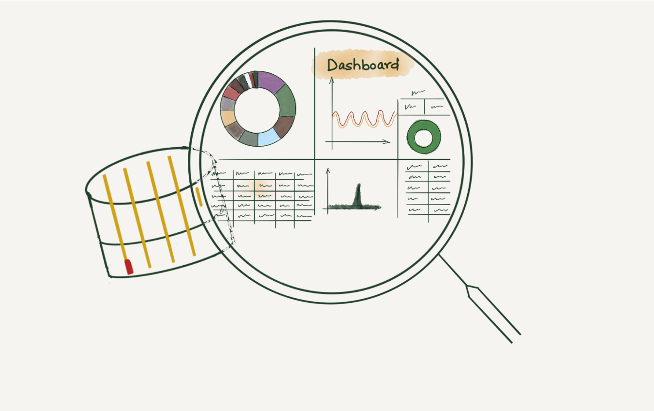
Observability aims to enhance insight into the technology stack by gathering and analyzing a broader spectrum of data. In this blog post, we delve into alert observability, discussing its importance and Cloudflare’s approach to achieving it. We’ll also explore how we overcome shortcomings in alert reporting within our architecture to simplify troubleshooting using open-source tools and best practices. Join us to understand how we use alerts effectively and use simple tools and practices to enhance our alerts observability, resilience, and on-call personnel health.

Being on-call can disrupt sleep patterns, impact social life, and hinder leisure activities, potentially leading to burnout. While burnout can be caused by several factors, one contributing factor can be excessively noisy alerts or receiving alerts that are neither important nor actionable. Analyzing alerts can help mitigate the risk of such burnout by reducing unnecessary interruptions and improving the overall efficiency of the on-call process. It involves periodic review and feedback to the system for improving alert quality. Unfortunately, only some companies or teams do alert analysis, even though it is essential information that every on-call or manager should have access to.

Alert analysis is useful for on-call personnel, enabling them to easily see which alerts have fired during their shift to help draft handover notes and not miss anything important. In addition, managers can generate reports from these stats to see the improvements over time, as well as helping assess on-call vulnerability to burnout. Alert analysis also helps with writing incident reports, to see if alerts were fired, or to determine when an incident started.

Let’s first understand the alerting stack and how we used open-source tools to gain greater visibility into it, which allowed us to analyze and optimize its effectiveness.

Prometheus architecture at Cloudflare

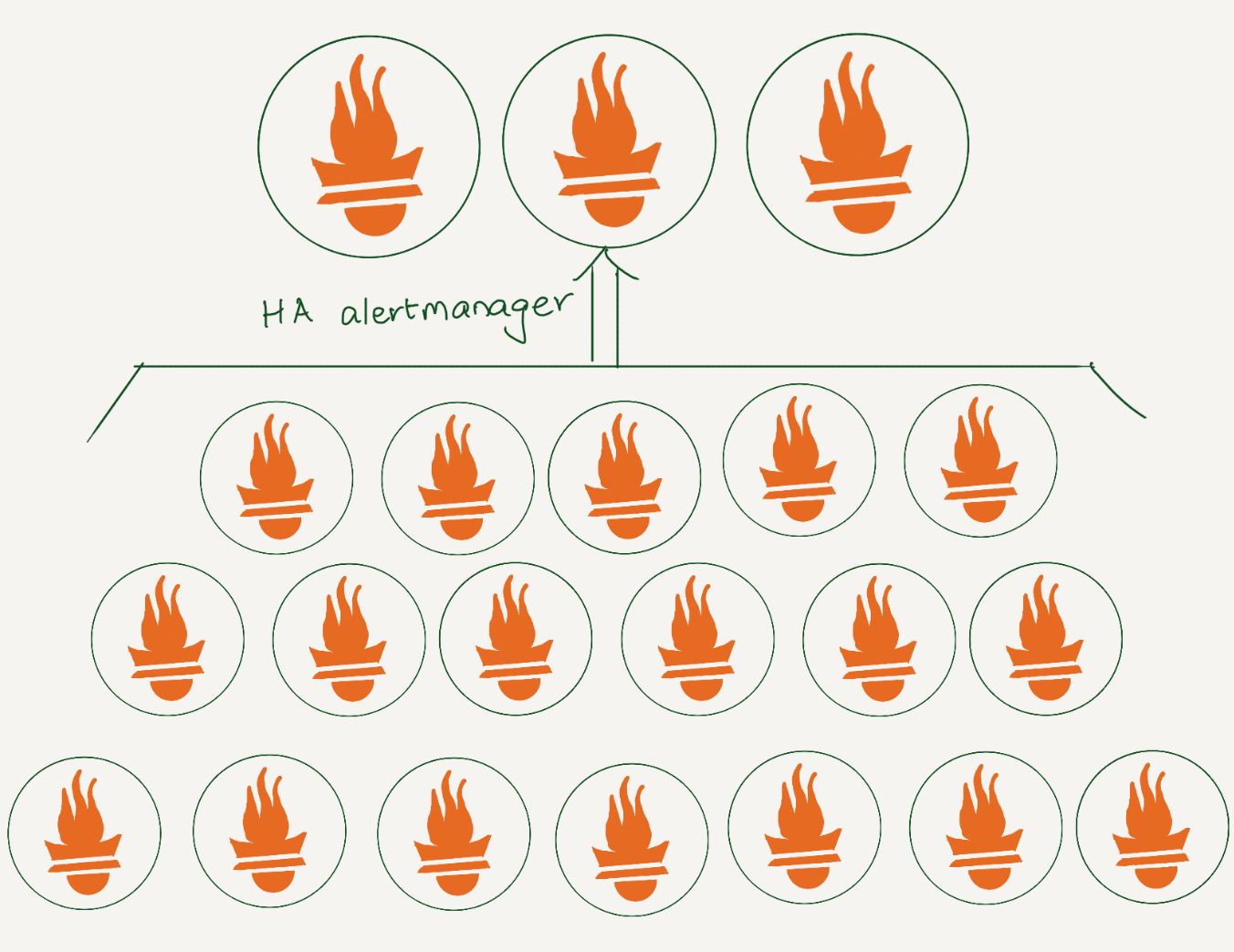
At Cloudflare, we rely heavily on Prometheus for monitoring. We have data centers in more than 310 cities, and each has several Prometheis. In total, we have over 1100 Prometheus servers. All alerts are sent to a central Alertmanager, where we have various integrations to route them. Additionally, using an alertmanager webhook, we store all alerts in a datastore for analysis.

Lifecycle of an alert

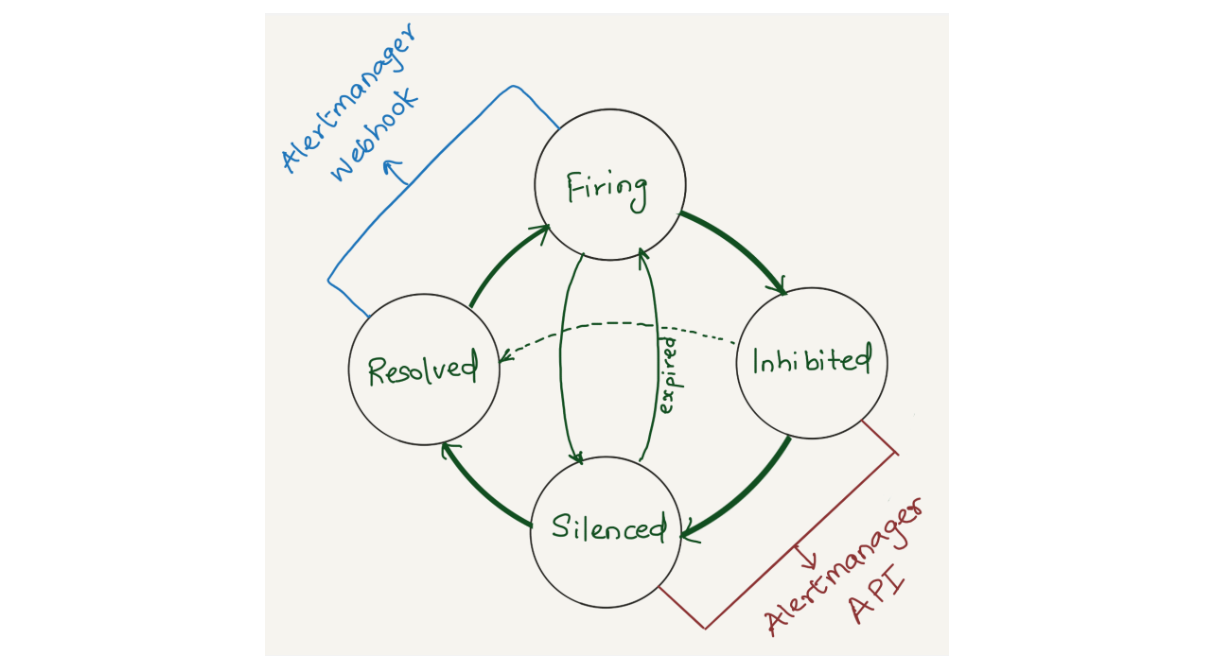
Prometheus collects metrics from configured targets at given intervals, evaluates rule expressions, displays the results, and can trigger alerts when the alerting conditions are met. Once an alert goes into firing state, it will be sent to the alertmanager.

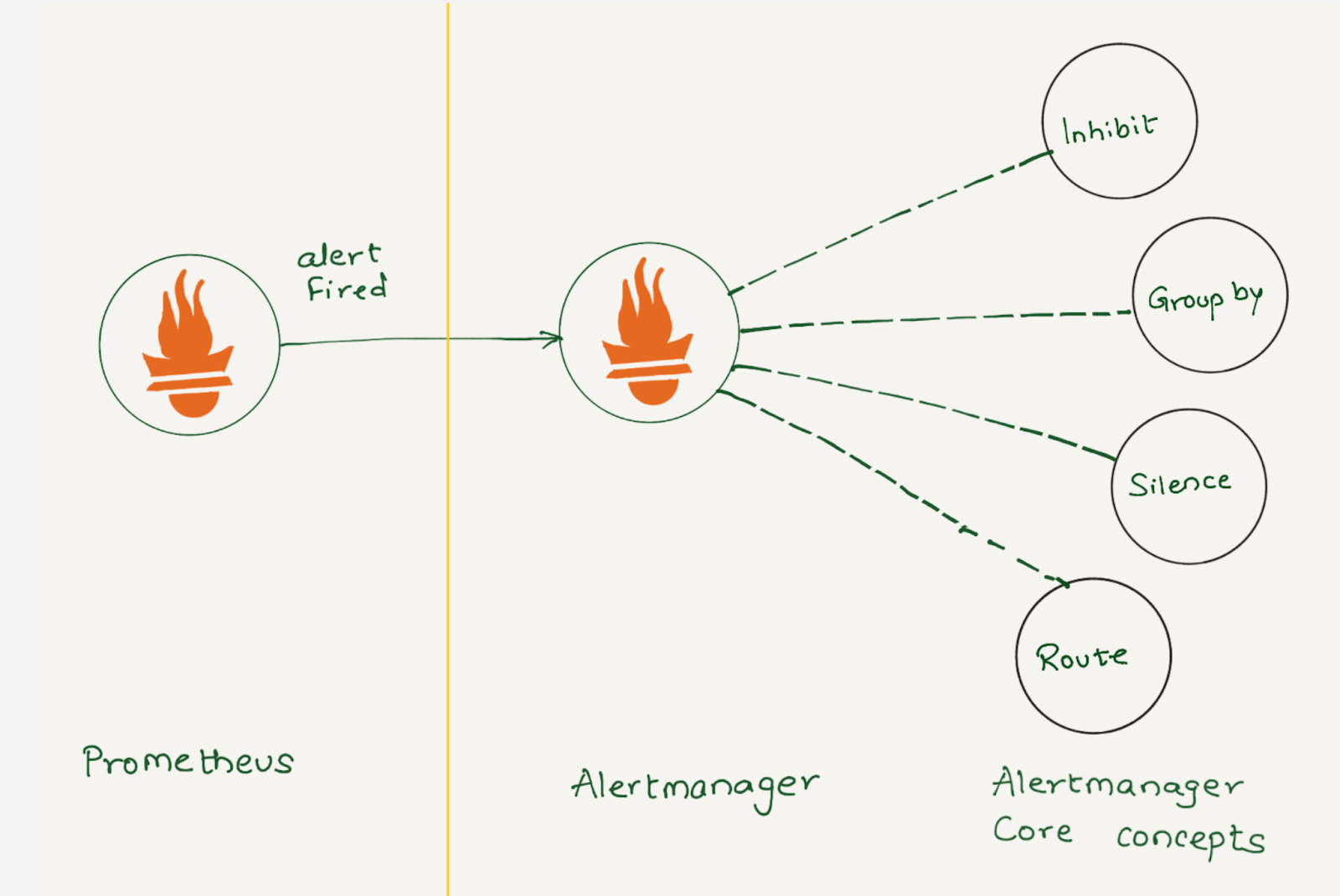
Depending on the configuration, once Alertmanager receives an alert, it can inhibit, group, silence, or route the alerts to the correct receiver integration, such as chat, PagerDuty, or ticketing system. When configured properly, Alertmanager can mitigate a lot of alert noise. Unfortunately, that is not the case all the time, as not all alerts are optimally configured.

In Alertmanager, alerts initially enter the firing state, where they may be inhibited or silenced. They return to the firing state when the silence expires or the inhibiting alert resolves, and eventually transition to the resolved state.

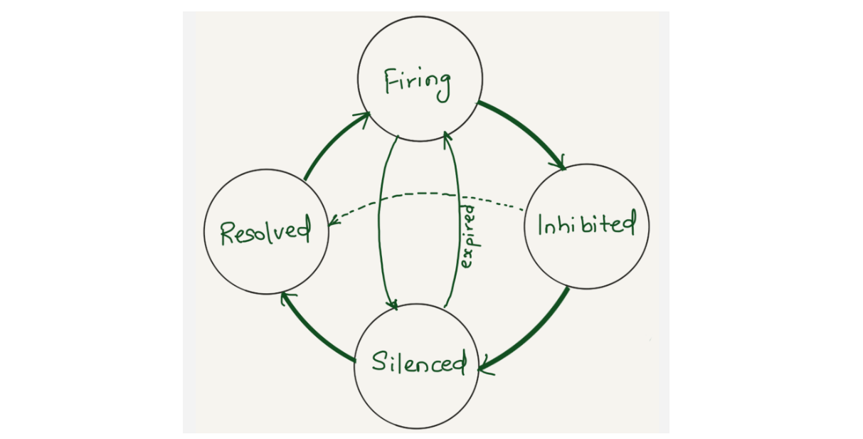
Alertmanager sends notifications for firing and resolved alert events via webhook integration. We were using alertmanager2es, which receives webhook alert notifications from Alertmanager and inserts them into an Elasticsearch index for searching and analysis. Alertmanager2es has been a reliable tool for us over the years, offering ways to monitor alerting volume, noisy alerts and do some kind of alert reporting. However, it had its limitations. The absence of silenced and inhibited alert states made troubleshooting issues challenging. We often found ourselves guessing why an alert didn’t trigger – was it silenced by another alert or perhaps inhibited by one? Without concrete data, we lacked the means to confirm what was truly happening.

Since the Alertmanager doesn’t provide notifications for silenced or inhibited alert events via webhook integration, the alert reporting we were doing was somewhat lacking or incomplete. However, the Alertmanager API provides querying capabilities and by querying the /api/alerts alertmanager endpoint, we can get the silenced and inhibited alert states. Having all four states in a datastore will enhance our ability to improve alert reporting and troubleshoot Alertmanager issues.

Interfaces for providing information about alert states

Solution

We opted to aggregate all states of the alerts (firing, silenced, inhibited, and resolved) into a datastore. Given that we’re gathering data from two distinct sources (the webhook and API) each in varying formats and potentially representing different events, we correlate alerts from both sources using the fingerprint field. The fingerprint is a unique hash of the alert’s label set which enables us to match alerts across responses from the Alertmanager webhook and API.

Alertmanager webhook and API response of same alert event

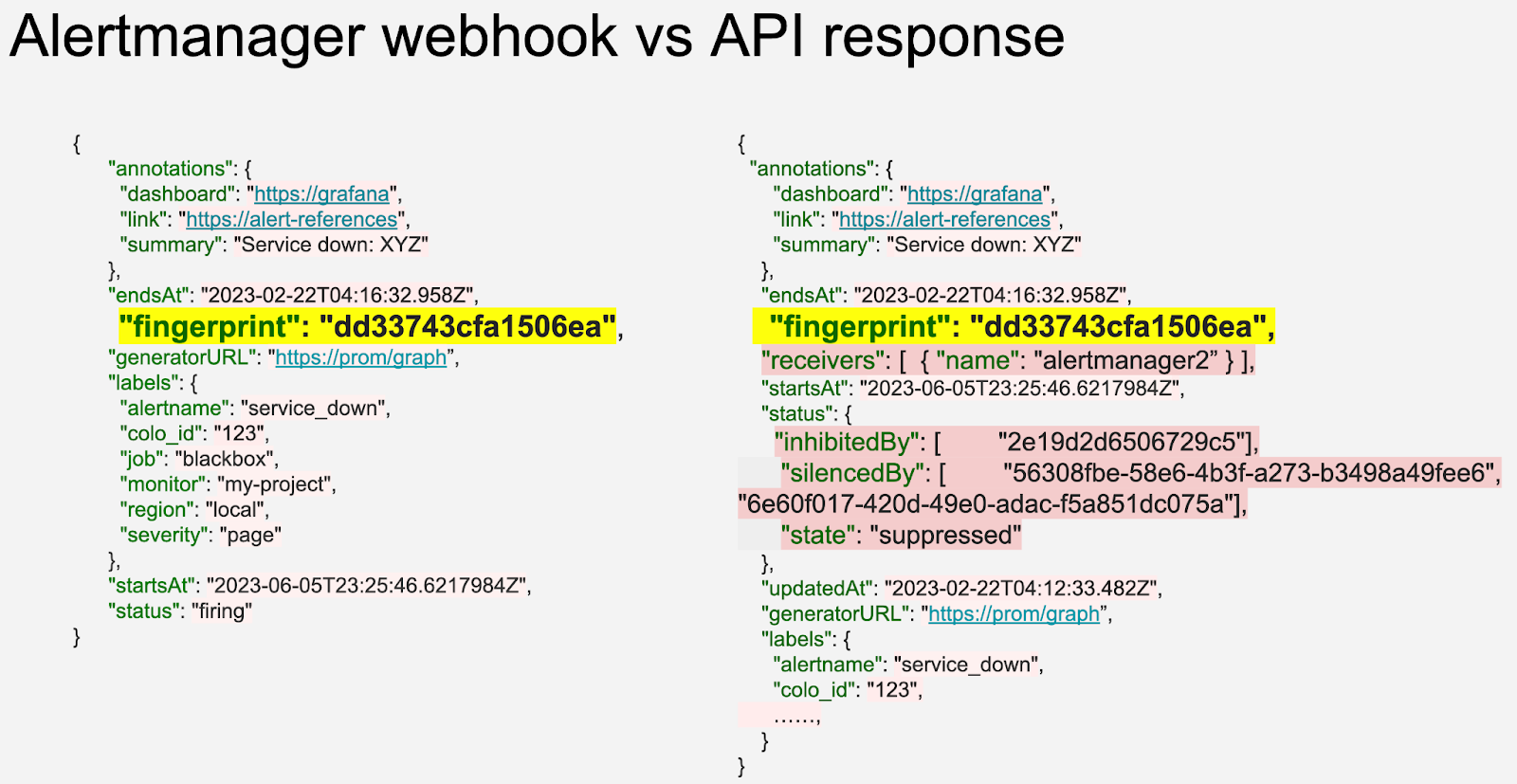
The Alertmanager API offers additional fields compared to the webhook (highlighted in pastel red on the right), such as silencedBy and inhibitedBy IDs, which aid in identifying silenced and inhibited alerts. We store both webhook and API responses in the datastore as separate rows. While querying, we match the alerts using the fingerprint field.

We decided to use a vector.dev instance to transform the data as necessary, and store it in a data store. Vector.dev (acquired by Datadog) is an open-source, high-performance, observability data pipeline that supports a vast range of sources to read data from and supports a lot of sinks for writing data to, as well as a variety of data transformation operations.

Here, we use one http_server vector instance to receive Alertmanager webhook notifications, two http_client sources to query alerts and silence API endpoints, and two sinks for writing all of the state logs in ClickHouse into alerts and silences tables

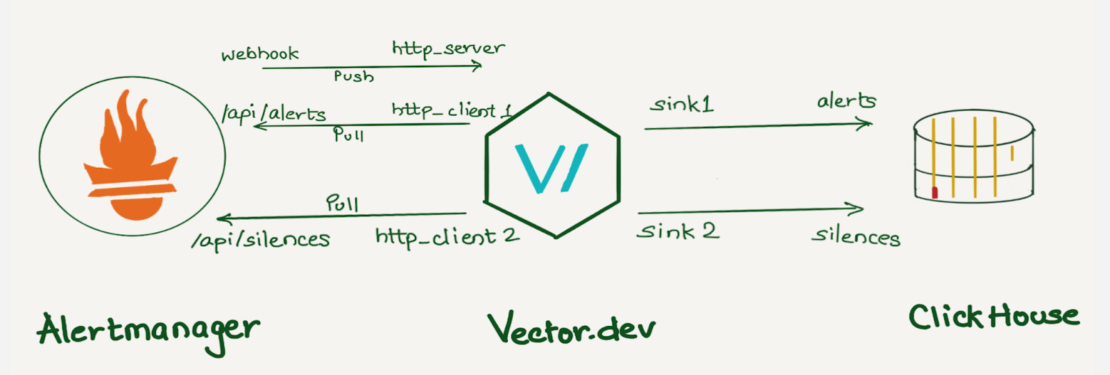
Although we use ClickHouse to store this data, any other database can be used here. ClickHouse was chosen as a data store because it provides various data manipulation options. It allows aggregating data during insertion using Materialized Views, reduces duplicates with the replacingMergeTree table engine, and supports JOIN statements.

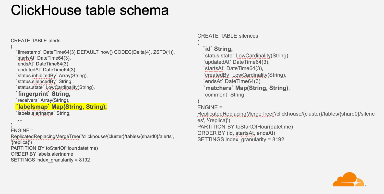
If we were to create individual columns for all the alert labels, the number of columns would grow exponentially with the addition of new alerts and unique labels. Instead, we decided to create individual columns for a few common labels like alert priority, instance, dashboard, alert-ref, alertname, etc., which helps us analyze the data in general and keep all other labels in a column of type Map(String, String). This was done because we wanted to keep all the labels in the datastore with minimal resource usage and allow users to query specific labels or filter alerts based on particular labels. For example, we can select all Prometheus alerts using  labelsmap[‘service’’] = ‘Prometheus’.

Dashboards

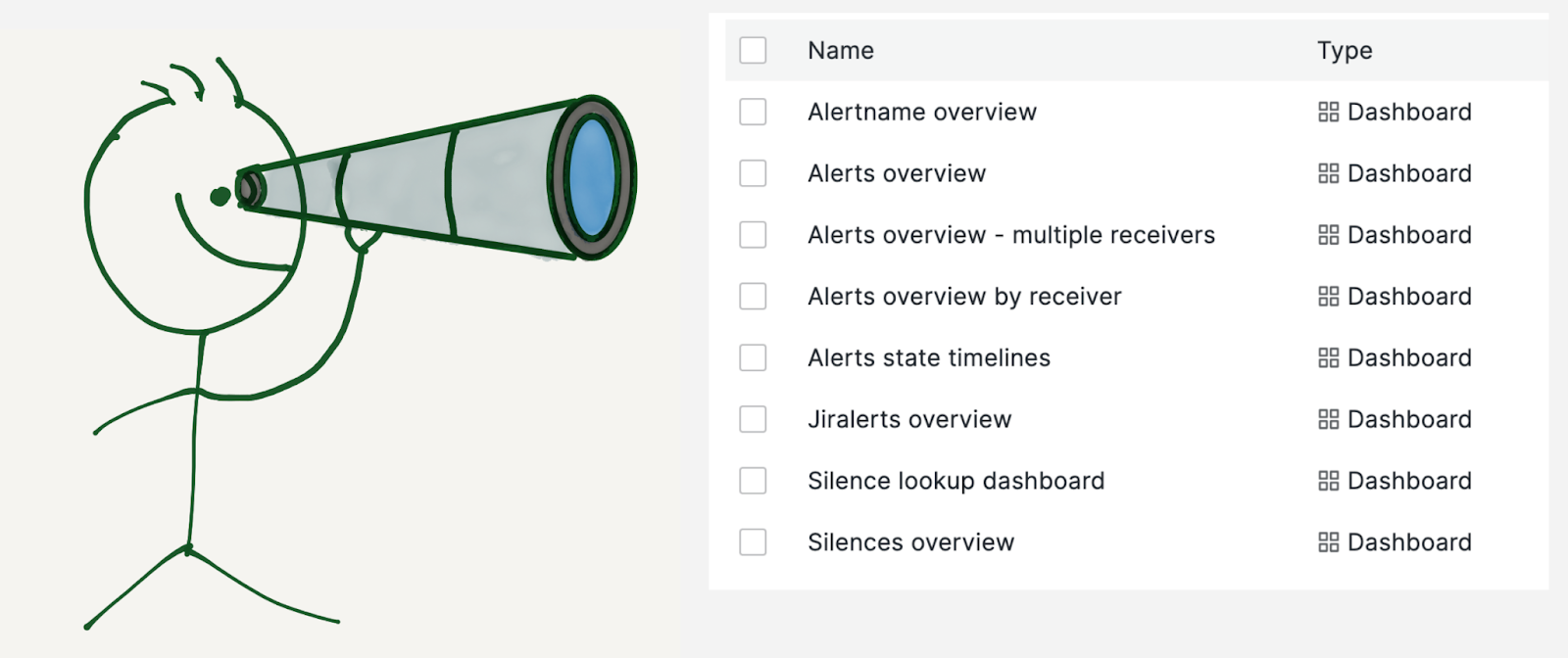
We built multiple dashboards on top of this data:

  • Alerts overview: To get insights into all the alerts the Alertmanager receives.
  • Alertname overview: To drill down on a specific alert.
  • Alerts overview by receiver: This is similar to alerts overview but specific to a team or receiver.
  • Alerts state timeline: This dashboard shows a snapshot of alert volume at a glance.
  • Jiralerts overview: To get insights into the alerts the ticket system receives.
  • Silences overview: To get insights into the Alertmanager silences.

Alerts overview

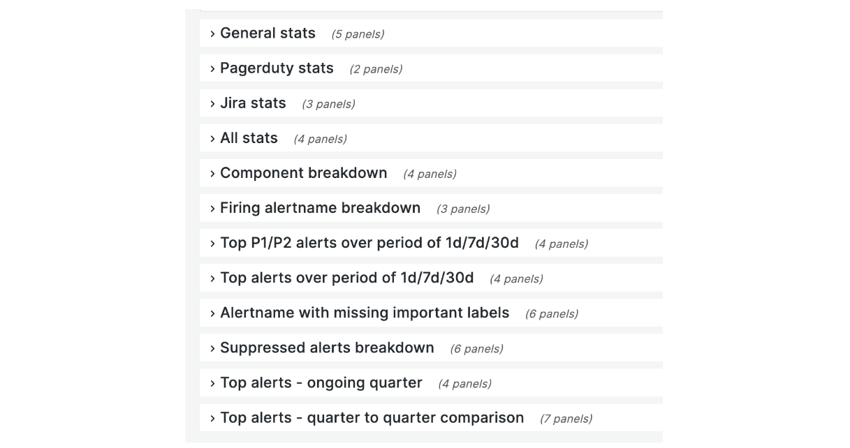
The image is a screenshot of the collapsed alerts overview dashboard by receiver. This dashboard comprises general stats, components, services, and alertname breakdown. The dashboard also highlights the number of P1 / P2 alerts in the last one day / seven days / thirty days, top alerts for the current quarter, and quarter-to-quarter comparison.

Component breakdown

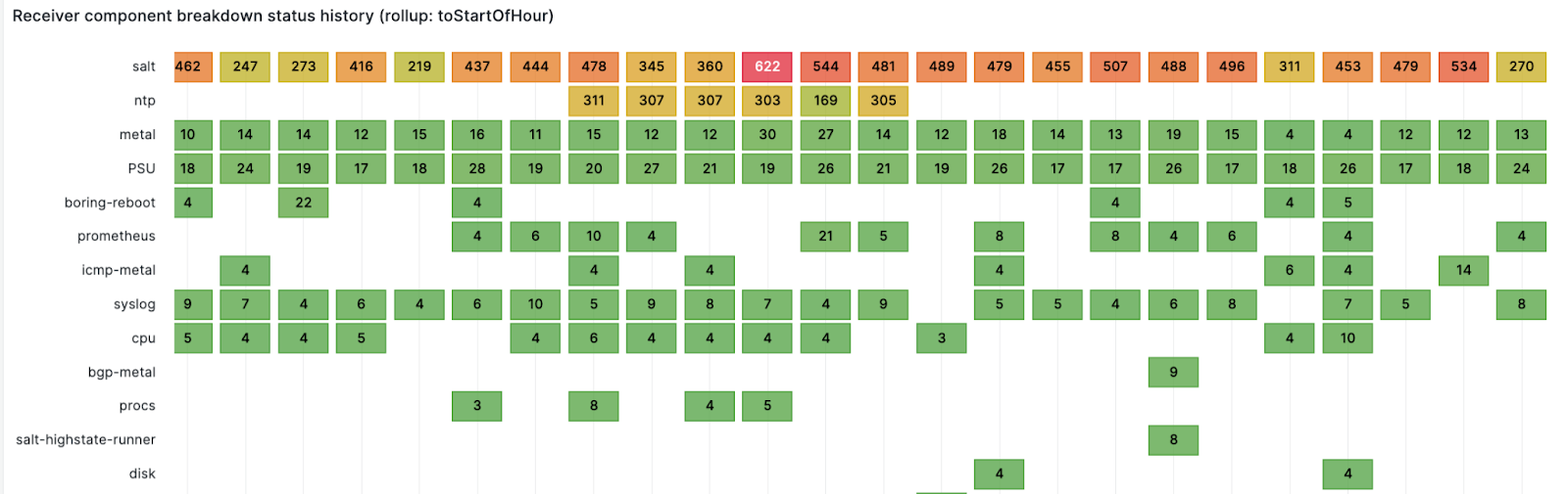
We route alerts to teams and a team can have multiple services or components. This panel shows firing alerts component counts over time for a receiver. For example, the alerts are sent to the observability team, which owns multiple components like logging, metrics, traces, and errors. This panel gives an alerting component count over time, and provides a good idea about which component is noisy and at what time at a glance.

Timeline of alerts

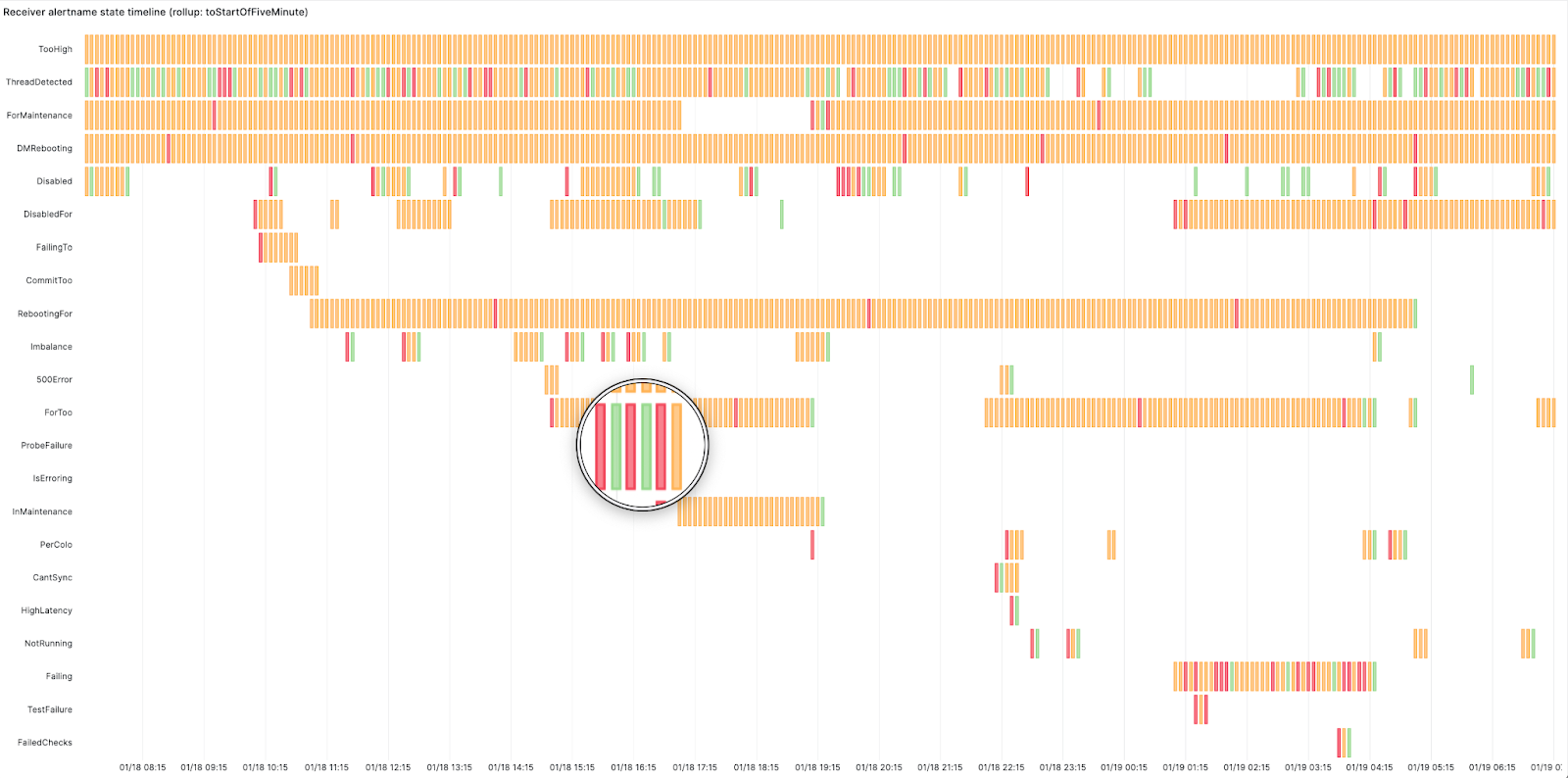
We created this swimlane view using Grafana’s state timeline panel for the receivers. The panel shows how busy the on-call was and at what point. Red here means the alert started firing, orange represents the alert is active and green means it has resolved. It displays the start time, active duration, and resolution of an alert. This highlighted alert is changing state too frequently from firing to resolved – this looks like a flapping alert. Flapping occurs when an alert changes state too frequently. This can happen when alerts are not configured properly and need tweaking, such as adjusting the alert threshold or increasing the for duration period in the alerting rule. The for duration field in the alerting rules adds time tolerance before an alert starts firing. In other words, the alert won’t fire unless the condition is met for ‘X’ minutes.

Findings

There were a few interesting findings within our analysis. We found a few alerts that were firing and did not have a notify label set, which means the alerts were firing but were not being sent or routed to any team, creating unnecessary load on the Alertmanager. We also found a few components generating a lot of alerts, and when we dug in, we found that they were for a cluster that was decommissioned where the alerts were not removed. These dashboards gave us excellent visibility and cleanup opportunities.

Alertmanager inhibitions

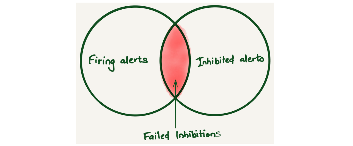
Alertmanager inhibition allows suppressing a set of alerts or notifications based on the presence of another set of alerts. We found that Alertmanager inhibitions were not working sometimes. Since there was no way to know about this, we only learned about it when a user reported getting alerted for inhibited alerts. Imagine a Venn diagram of firing and inhibited alerts to understand failed inhibitions. Ideally, there should be no overlap because the inhibited alerts shouldn’t be firing. But if there is an overlap, that means inhibited alerts are firing, and this overlap is considered a failed inhibition alert.

Failed inhibition venn diagram

After storing alert notifications in ClickHouse, we were able to come up with a query to find the fingerprint of the `alertnames` where the inhibitions were failing using the following query:

SELECT $rollup(timestamp) as t, count() as count
FROM
(
    SELECT
        fingerprint, timestamp
    FROM alerts
    WHERE
        $timeFilter
        AND status.state = 'firing'
    GROUP BY
        fingerprint, timestamp
) AS firing
ANY INNER JOIN
(
    SELECT
        fingerprint, timestamp
    FROM alerts
    WHERE
        $timeFilter
        AND status.state = 'suppressed' AND notEmpty(status.inhibitedBy)
    GROUP BY
        fingerprint, timestamp
) AS suppressed USING (fingerprint)
GROUP BY t

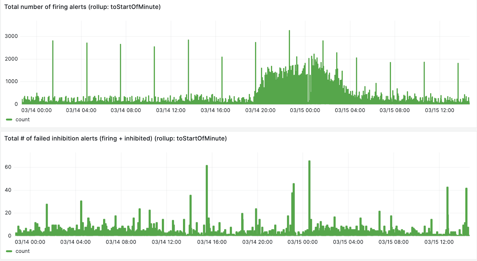
The first panel in the image below is the total number of firing alerts, the second panel is the number of failed inhibitions.

We can also create breakdown for each failed inhibited alert

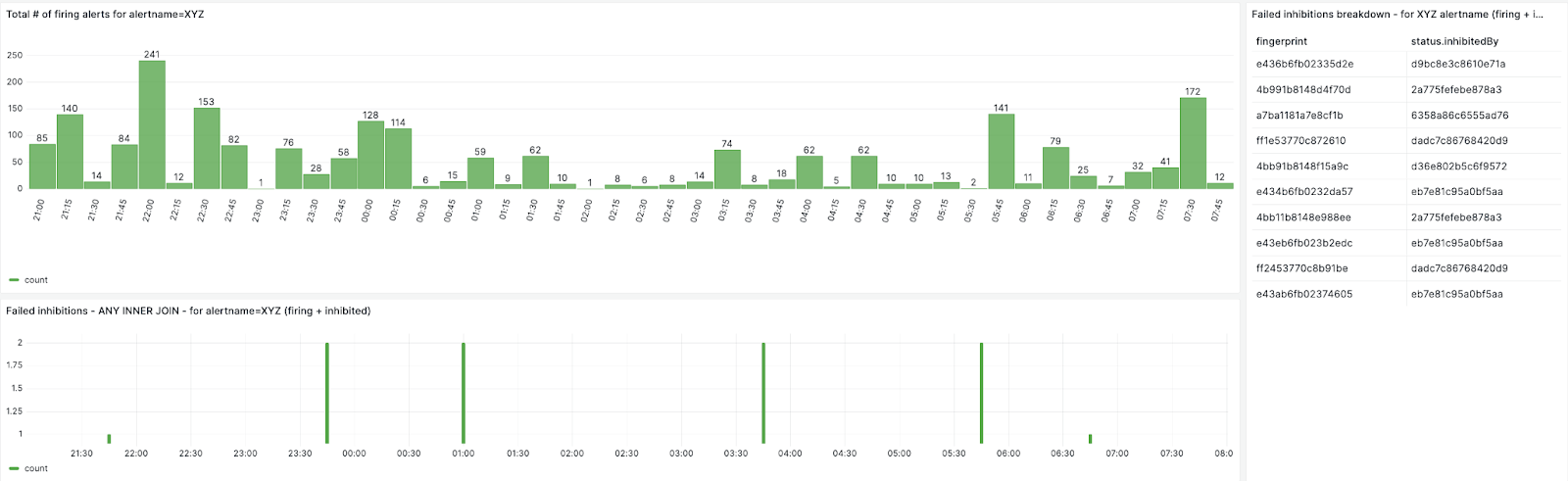
By looking up the fingerprint from the database, we could map the alert inhibitions and found that the failed inhibited alerts have an inhibition loop. For example, alert Service_XYZ_down is inhibited by alert server_OOR, alert server_OOR is inhibited by alert server_down, and server_down is inhibited by alert server_OOR.

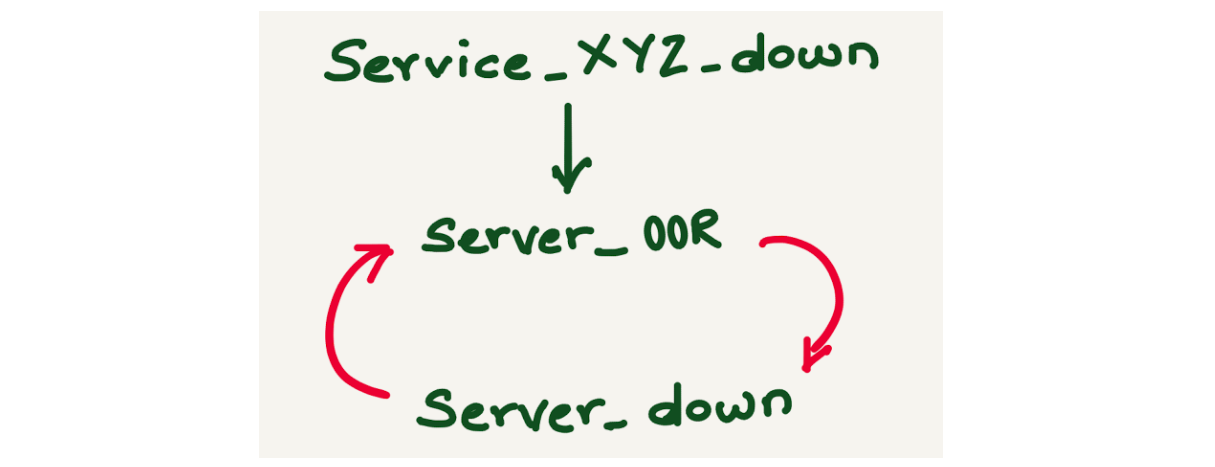
Failed inhibitions can be avoided if alert inhibitions are configured carefully.

Silences

Alertmanager provides a mechanism to silence an alert while it is being worked on or during maintenance. Silence can mute the alerts for a given time and it can be configured based on matchers, which can be an exact match, a regex, an alert name, or any other label. The silence matcher doesn’t necessarily translate to the alertname. By doing alert analysis, we could map the alerts and the silence ID by doing a JOIN query on the alerts and silences tables. We also discovered a lot of stale silences, where silence was created for a long duration and is not relevant anymore.

DIY Alert analysis

The directory contains a basic demo for implementing alerts observability. Running `docker-compose up` spawns several containers, including Prometheus, Alertmanager, Vector, ClickHouse, and Grafana. The vector.dev container queries the Alertmanager alerts API and writes the data into ClickHouse after transforming it. The Grafana dashboard showcases a demo of Alerts and Silences overview.

Make sure you have docker installed and run docker compose up to get started.

Visit http://localhost:3000/dashboards to explore the prebuilt demo dashboards.

Conclusion

As part of the observability team, we manage the Alertmanager, which is a multi-tenant system. It’s crucial for us to have visibility to detect and address system misuse, ensuring proper alerting. The use of alert analysis tools has significantly enhanced the experience for on-call personnel and our team, offering swift access to the alert system. Alerts observability has facilitated the troubleshooting of events such as why an alert did not fire, why an inhibited alert fired, or which alert silenced / inhibited another alert, providing valuable insights for improving alert management.

Moreover, alerts overview dashboards facilitate rapid review and adjustment, streamlining operations. Teams use these dashboards in the weekly alert reviews to provide tangible evidence of how an on-call shift went, identify which alerts fire most frequently, becoming candidates for cleanup or aggregation thus curbing system misuse and bolstering overall alert management. Additionally, we can pinpoint services that may require particular attention. Alerts observability has also empowered some teams to make informed decisions about on-call configurations, such as transitioning to longer but less frequent shifts or integrating on-call and unplanned work shifts.

In conclusion, alert observability plays a crucial role in averting burnout by minimizing interruptions and enhancing on-call duties’ efficiency. Offering alerts observability as a service benefits all teams by obviating the need for individual dashboard development and fostering a proactive monitoring culture.
If you found this blog post interesting and want to work on observability, please check out our job openings – we’re hiring for Alerting and Logging!

Log analytics using ClickHouse

Post Syndicated from Monika Singh original https://blog.cloudflare.com/log-analytics-using-clickhouse/

Log analytics using ClickHouse

This is an adapted transcript of a talk we gave at Monitorama 2022. You can find the slides with presenter’s notes here and video here.

Log analytics using ClickHouse

When a request at Cloudflare throws an error, information gets logged in our requests_error pipeline. The error logs are used to help troubleshoot customer-specific or network-wide issues.

We, Site Reliability Engineers (SREs), manage the logging platform. We have been running Elasticsearch clusters for many years and during these years, the log volume has increased drastically. With the log volume increase, we started facing a few issues. Slow query performance and high resource consumption to list a few. We aimed to improve the log consumer’s experience by improving query performance and providing cost-effective solutions for storing logs. This blog post discusses challenges with logging pipelines and how we designed the new architecture to make it faster and cost-efficient.

Before we dive into challenges in maintaining the logging pipelines, let us look at the characteristics of logs.

Characteristics of logs

Log analytics using ClickHouse

Unpredictable – In today’s world, where there are tons of microservices, the amount of logs a centralized logging system will receive is very unpredictable. There are various reasons why capacity estimation of log volume is so difficult. Primarily because new applications get deployed to production continuously, existing applications are automatically scaled up or down to handle business demands or sometimes application owners enable debug log levels and forget to turn it off.

Semi-structured – Every application adopts a different logging format. Some are represented in plain-text and others use JSON. The timestamp field within these log lines also varies. Multi-line exceptions and stack traces make them even more unstructured. Such logs add extra resource overhead, requiring additional data parsing and mangling.

Contextual – For debugging issues, often contextual information is required, that is, logs before and after an event happened. A single logline hardly helps, generally, it’s the group of loglines that helps in building the context. Also, we often need to correlate the logs from multiple applications to draw the full picture. Hence it’s essential to preserve the order in which logs get populated at the source.

Write-heavy – Any centralized logging system is write-intensive. More than 99% of logs that are written, are never read. They occupy space for some time and eventually get purged by the retention policies. The remaining less than 1% of the logs that are read are very important and we can’t afford to miss them.

Logging pipeline

Like most other companies, our logging pipeline consists of a producer, shipper, a queue, a consumer and a datastore.

Log analytics using ClickHouse

Applications (Producers) running on the Cloudflare global network generate the logs. These logs are written locally in Cap’n Proto serialized format. The Shipper (in-house solution) pushes the Cap’n Proto serialized logs through streams for processing to Kafka (queue). We run Logstash (consumer), which consumes from Kafka and writes the logs into ElasticSearch (datastore).The data is then visualized by using Kibana or Grafana. We have multiple dashboards built in both Kibana and Grafana to visualize the data.

Elasticsearch bottlenecks at Cloudflare

At Cloudflare, we have been running Elasticsearch clusters for many years. Over the years, log volume increased dramatically and while optimizing our Elasticsearch clusters to handle such volume, we found a few limitations.

Mapping Explosion

Log analytics using ClickHouse

Mapping Explosion is one of the very well-known limitations of Elasticsearch. Elasticsearch maintains a mapping that decides how a new document and its fields are stored and indexed. When there are too many keys in this mapping, it can take a significant amount of memory resulting in frequent garbage collection. One way to prevent this is to make the schema strict, which means any log line not following this strict schema will end up getting dropped. Another way is to make it semi-strict, which means any field not part of this mapping will not be searchable.

Multi-tenancy support

Log analytics using ClickHouse

Elasticsearch doesn’t have very good multi-tenancy support. One bad user can easily impact cluster performance. There is no way to limit the maximum number of documents or indexes a query can read or the amount of memory an Elasticsearch query can take. A bad query can easily degrade cluster performance and even after the query finishes, it can still leave its impact.

Cluster operational tasks

It is not easy to manage Elasticsearch clusters, especially multi-tenant ones. Once a cluster degrades, it takes significant time to get the cluster back to a fully healthy state. In Elasticsearch, updating the index template means reindexing the data, which is quite an overhead. We use hot and cold tiered storage, i.e., recent data in SSD and older data in magnetic drives. While Elasticsearch moves the data from hot to cold storage every day, it affects the read and write performance of the cluster.

Garbage collection

Log analytics using ClickHouse

Elasticsearch is developed in Java and runs on a Java Virtual Machine (JVM). It performs garbage collection to reclaim memory that was allocated by the program but is no longer referenced. Elasticsearch requires garbage collection tuning. The default garbage collection in the latest JVM is G1GC. We tried other GC like ZGC, which helped in lowering the GC pause but didn’t give us much performance benefit in terms of read and write throughput.

Log analytics using ClickHouse

Elasticsearch is a good tool for full-text search and these limitations are not significant with small clusters, but in Cloudflare, we handle over 35 to 45 million HTTP requests per second, out of which over 500K-800K requests fail per second. These failures can be due to an improper request, origin server errors, misconfigurations by users, network issues and various other reasons.

Our customer support team uses these error logs as the starting point to triage customer issues. The error logs have a number of fields metadata about various Cloudflare products that HTTP requests have been through. We were storing these error logs in Elasticsearch. We were heavily sampling them since storing everything was taking a few hundreds of terabytes crossing our resource allocation budget. Also, dashboards built over it were quite slow since they required heavy aggregation over various fields. We need to retain these logs for a few weeks per the debugging requirements.

Proposed solution

We wanted to remove sampling completely, that is, store every log line for the retention period, to provide fast query support over this huge amount of data and to achieve all this without increasing the cost.

To solve all these problems, we decided to do a proof of concept and see if we could accomplish our requirements using ClickHouse.

Cloudflare was an early adopter of ClickHouse and we have been managing ClickHouse clusters for years. We already had a lot of in-house tooling and libraries for inserting data into ClickHouse, which made it easy for us to do the proof of concept. Let us look at some of the ClickHouse features that make it the perfect fit for storing logs and which enabled us to build our new logging pipeline.

Log analytics using ClickHouse

ClickHouse is a column-oriented database which means all data related to a particular column is physically stored next to each other. Such data layout helps in fast sequential scan even on commodity hardware. This enabled us to extract maximum performance out of older generation hardware.

Log analytics using ClickHouse

ClickHouse is designed for analytical workloads where the data has a large number of fields that get represented as ClickHouse columns. We were able to design our new ClickHouse tables with a large number of columns without sacrificing performance.

Log analytics using ClickHouse

ClickHouse indexes work differently than those in relational databases. In relational databases, the primary indexes are dense and contain one entry per table row. So if you have 1 million rows in the table, the primary index will also have 1 million entries. While In ClickHouse, indexes are sparse, which means there will be only one index entry per a few thousand table rows. ClickHouse indexes enabled us to add new indexes on the fly.

ClickHouse compresses everything with LZ4 by default. An efficient compression not only helps in minimizing the storage needs but also lets ClickHouse use page cache efficiently.

One of the cool features of ClickHouse is that the compression codecs can be configured on a per-column basis. We decided to keep default LZ4 compression for all columns. We used special encodings like Double-Delta for the DateTime columns, Gorilla for Float columns and LowCardinality for fixed-size String columns.

ClickHouse is linearly scalable; that is, the writes can be scaled by adding new shards and the reads can be scaled by adding new replicas. Every node in a ClickHouse cluster is identical. Not having any special nodes helps in scaling the cluster easily.

Let’s look at some optimizations we leveraged to provide faster read/write throughput and better compression on log data.

Inserter

Having an efficient inserter is as important as having an efficient data store. At Cloudflare, we have been operating quite a few analytics pipelines from where we borrowed most of the concepts while writing our new inserter. We use Cap’n Proto messages as the transport data format since it provides fast data encoding and decoding. Scaling inserters is easy and can be done by adding more Kafka partitions and spawning new inserter pods.

Log analytics using ClickHouse

Batch Size

One of the key performance factors while inserting data into ClickHouse is the batch size. When batches are small, ClickHouse creates many small partitions, which it then merges into bigger ones. Thus smaller batch size creates extra work for ClickHouse to do in the background, thereby reducing ClickHouse’s performance. Hence it is crucial to set it big enough that ClickHouse can accept the data batch happily without hitting memory limits.

Log analytics using ClickHouse

Data modeling in ClickHouse.

ClickHouse provides in-built sharding and replication without any external dependency. Earlier versions of ClickHouse depended on ZooKeeper for storing replication information, but the recent version removed the ZooKeeper dependency by adding clickhouse-keeper.

To read data across multiple shards, we use distributed tables, a special kind of table. These tables don’t store any data themselves but act as a proxy over multiple underlying tables storing the actual data.

Log analytics using ClickHouse

Like any other database, choosing the right table schema is very important since it will directly impact the performance and storage utilization. We would like to discuss three ways you can store log data into ClickHouse.

Log analytics using ClickHouse

The first is the simplest and the most strict table schema where you specify every column name and data type. Any logline having a field outside this predefined schema will get dropped. From our experience, this schema will give you the fastest query capabilities. If you already know the list of all possible fields ahead, we would recommend using it. You can always add or remove columns by running ALTER TABLE queries.

The second schema uses a very new feature of ClickHouse, where it does most of the heavy lifting. You can insert logs as JSON objects and behind the scenes, ClickHouse will understand your log schema and dynamically add new columns with appropriate data type and compression. This schema should only be used if you have good control over the log schema and the number of total fields is less than 1,000. On the one hand it provides flexibility to add new columns as new log fields automatically, but at the same time, one lousy application can easily bring down the ClickHouse cluster.

The third schema stores all fields of the same data type in one array and then uses ClickHouse inbuilt array functions to query those fields. This schema scales pretty well even when there are more than 1,000 fields, as the number of columns depends on the data types used in the logs. If an array element is accessed frequently, it can be taken out as a dedicated column using the materialized column feature of ClickHouse. We recommend adopting this schema since it provides safeguards against applications logging too many fields.

Data partitioning

Log analytics using ClickHouse

A partition is a unit of ClickHouse data. One common mistake ClickHouse users make is overly granular partitioning keys, resulting in too many partitions. Since our logging pipeline generates TBs of data daily, we created the table partitioned with `toStartOfHour(dateTime).` With this partitioning logic, when a query comes with the timestamp in the WHERE clause, ClickHouse knows the partition and retrieves it quickly. It also helps design efficient data purging rules according to the data retention policies.

Primary key selection

Log analytics using ClickHouse

ClickHouse stores the data on disk sorted by primary key. Thus, selecting the primary key impacts the query performance and helps in better data compression. Unlike relational databases, ClickHouse doesn’t require a unique primary key per row and we can insert multiple rows with identical primary keys. Having multiple primary keys will negatively impact the insertion performance. One of the significant ClickHouse limitations is that once a table is created the primary key can not be updated.

Data skipping indexes

Log analytics using ClickHouse

ClickHouse query performance is directly proportional to whether it can use the primary key when evaluating the WHERE clause. We have many columns and all these columns can not be part of the primary key. Thus queries on these columns will have to do a full scan resulting in slower queries. In traditional databases, secondary indexes can be added to handle such situations. In ClickHouse, we can add another class of indexes called data skipping indexes, which uses bloom filters and skip reading significant chunks of data that are guaranteed to have no match.

ABR

We have multiple dashboards built over the requests_error logs. Loading these dashboards were often hitting the memory limits set for the individual query/user in ClickHouse.

The dashboards built over these logs were mainly used to identify anomalies. To visually identify an anomaly in a metric, the exact numbers are not required, but an approximate number would do. For instance, to understand that errors have increased in a data center, we don’t need the exact number of errors. So we decided to use an in-house library and tool built around a concept called ABR.

Log analytics using ClickHouse

ABR stands for “Adaptive Bit Rate” – the term ABR is mainly used in video streaming services where servers select the best resolution for a video stream to match the client and network connection. It is described in great detail in the blog post – Explaining Cloudflare’s ABR Analytics

In other words, the data is stored at multiple resolutions or sample intervals and the best solution is picked for each query.

The way ABR works is at the time of writing requests to ClickHouse, it writes the data in a number of tables with different sample intervals. For instance table_1 stores 100% of data, table_10 stores 10% of data, table_100 stores 1% of data and table_1000 stores 0.1% data so on and so forth. The data is duplicated between the tables. Table_10 would be a subset of table_1.

Demo

In Cloudflare, we use in-house libraries and tools to insert data into ClickHouse, but this can be achieved by using an open source tool – vector.dev

If you would like to test how log ingestion into ClickHouse works, you can refer or use the demo here.

Make sure you have docker installed and run `docker compose up` to get started.

This would bring up three containers, Vector.dev for generating vector demo logs, writing it into ClickHouse, ClickHouse container to store the logs and Grafana instance to visualize the logs.

When the containers are up, visit http://localhost:3000/dashboards to play with the prebuilt demo dashboard.

Conclusion

Log analytics using ClickHouse

Logs are supposed to be immutable by nature and ClickHouse works best with immutable data. We were able to migrate one of the critical and significant log-producing applications from Elasticsearch to a much smaller ClickHouse cluster.

CPU and memory consumption on the inserter side were reduced by eight times. Each Elasticsearch document which used 600 bytes, came down to 60 bytes per row in ClickHouse. This storage gain allowed us to store 100% of the events in a newer setup. On the query side, the 99th percentile of the query latency also improved drastically.

Elasticsearch is great for full-text search and ClickHouse is great for analytics.