Tag Archives: ClickHouse

Log analytics using ClickHouse

2022-09-02 Monika Singh

Post Syndicated from Monika Singh original https://blog.cloudflare.com/log-analytics-using-clickhouse/

Log analytics using ClickHouse

This is an adapted transcript of a talk we gave at Monitorama 2022. You can find the slides with presenter’s notes here and video here.

When a request at Cloudflare throws an error, information gets logged in our requests_error pipeline. The error logs are used to help troubleshoot customer-specific or network-wide issues.

We, Site Reliability Engineers (SREs), manage the logging platform. We have been running Elasticsearch clusters for many years and during these years, the log volume has increased drastically. With the log volume increase, we started facing a few issues. Slow query performance and high resource consumption to list a few. We aimed to improve the log consumer’s experience by improving query performance and providing cost-effective solutions for storing logs. This blog post discusses challenges with logging pipelines and how we designed the new architecture to make it faster and cost-efficient.

Before we dive into challenges in maintaining the logging pipelines, let us look at the characteristics of logs.

Characteristics of logs

Unpredictable – In today’s world, where there are tons of microservices, the amount of logs a centralized logging system will receive is very unpredictable. There are various reasons why capacity estimation of log volume is so difficult. Primarily because new applications get deployed to production continuously, existing applications are automatically scaled up or down to handle business demands or sometimes application owners enable debug log levels and forget to turn it off.

Semi-structured – Every application adopts a different logging format. Some are represented in plain-text and others use JSON. The timestamp field within these log lines also varies. Multi-line exceptions and stack traces make them even more unstructured. Such logs add extra resource overhead, requiring additional data parsing and mangling.

Contextual – For debugging issues, often contextual information is required, that is, logs before and after an event happened. A single logline hardly helps, generally, it’s the group of loglines that helps in building the context. Also, we often need to correlate the logs from multiple applications to draw the full picture. Hence it’s essential to preserve the order in which logs get populated at the source.

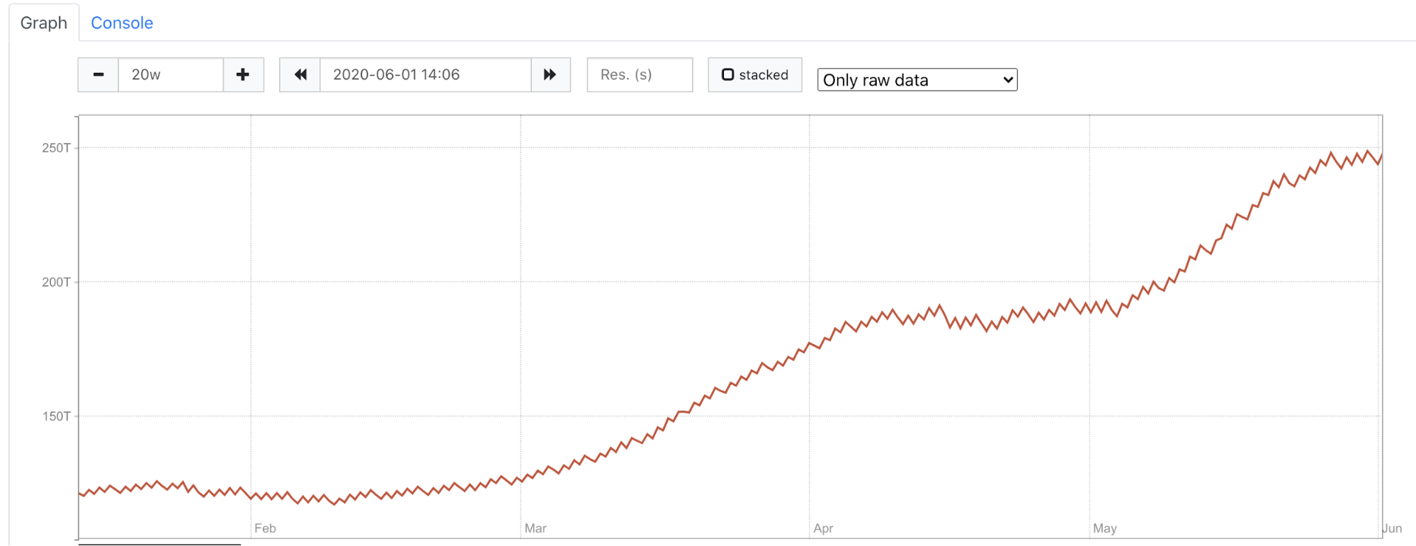
Write-heavy – Any centralized logging system is write-intensive. More than 99% of logs that are written, are never read. They occupy space for some time and eventually get purged by the retention policies. The remaining less than 1% of the logs that are read are very important and we can’t afford to miss them.

Logging pipeline

Like most other companies, our logging pipeline consists of a producer, shipper, a queue, a consumer and a datastore.

Applications (Producers) running on the Cloudflare global network generate the logs. These logs are written locally in Cap’n Proto serialized format. The Shipper (in-house solution) pushes the Cap’n Proto serialized logs through streams for processing to Kafka (queue). We run Logstash (consumer), which consumes from Kafka and writes the logs into ElasticSearch (datastore).The data is then visualized by using Kibana or Grafana. We have multiple dashboards built in both Kibana and Grafana to visualize the data.

Elasticsearch bottlenecks at Cloudflare

At Cloudflare, we have been running Elasticsearch clusters for many years. Over the years, log volume increased dramatically and while optimizing our Elasticsearch clusters to handle such volume, we found a few limitations.

Mapping Explosion

Mapping Explosion is one of the very well-known limitations of Elasticsearch. Elasticsearch maintains a mapping that decides how a new document and its fields are stored and indexed. When there are too many keys in this mapping, it can take a significant amount of memory resulting in frequent garbage collection. One way to prevent this is to make the schema strict, which means any log line not following this strict schema will end up getting dropped. Another way is to make it semi-strict, which means any field not part of this mapping will not be searchable.

Multi-tenancy support

Elasticsearch doesn’t have very good multi-tenancy support. One bad user can easily impact cluster performance. There is no way to limit the maximum number of documents or indexes a query can read or the amount of memory an Elasticsearch query can take. A bad query can easily degrade cluster performance and even after the query finishes, it can still leave its impact.

Cluster operational tasks

It is not easy to manage Elasticsearch clusters, especially multi-tenant ones. Once a cluster degrades, it takes significant time to get the cluster back to a fully healthy state. In Elasticsearch, updating the index template means reindexing the data, which is quite an overhead. We use hot and cold tiered storage, i.e., recent data in SSD and older data in magnetic drives. While Elasticsearch moves the data from hot to cold storage every day, it affects the read and write performance of the cluster.

Garbage collection

Elasticsearch is developed in Java and runs on a Java Virtual Machine (JVM). It performs garbage collection to reclaim memory that was allocated by the program but is no longer referenced. Elasticsearch requires garbage collection tuning. The default garbage collection in the latest JVM is G1GC. We tried other GC like ZGC, which helped in lowering the GC pause but didn’t give us much performance benefit in terms of read and write throughput.

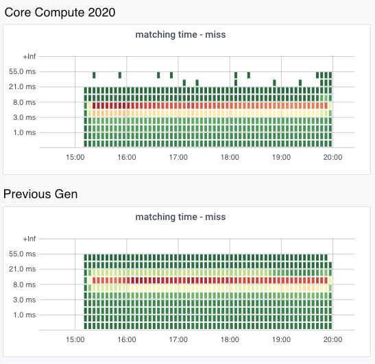
Elasticsearch is a good tool for full-text search and these limitations are not significant with small clusters, but in Cloudflare, we handle over 35 to 45 million HTTP requests per second, out of which over 500K-800K requests fail per second. These failures can be due to an improper request, origin server errors, misconfigurations by users, network issues and various other reasons.

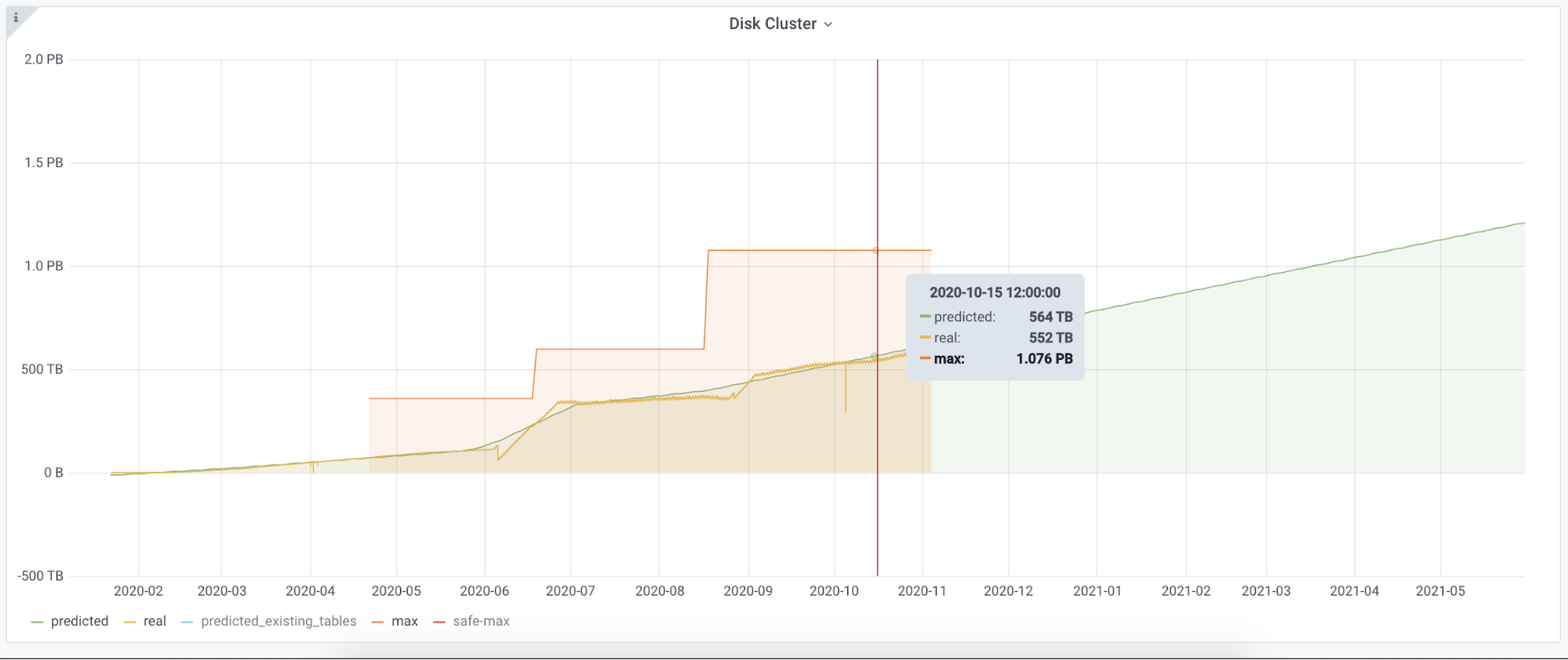
Our customer support team uses these error logs as the starting point to triage customer issues. The error logs have a number of fields metadata about various Cloudflare products that HTTP requests have been through. We were storing these error logs in Elasticsearch. We were heavily sampling them since storing everything was taking a few hundreds of terabytes crossing our resource allocation budget. Also, dashboards built over it were quite slow since they required heavy aggregation over various fields. We need to retain these logs for a few weeks per the debugging requirements.

Proposed solution

We wanted to remove sampling completely, that is, store every log line for the retention period, to provide fast query support over this huge amount of data and to achieve all this without increasing the cost.

To solve all these problems, we decided to do a proof of concept and see if we could accomplish our requirements using ClickHouse.

Cloudflare was an early adopter of ClickHouse and we have been managing ClickHouse clusters for years. We already had a lot of in-house tooling and libraries for inserting data into ClickHouse, which made it easy for us to do the proof of concept. Let us look at some of the ClickHouse features that make it the perfect fit for storing logs and which enabled us to build our new logging pipeline.

ClickHouse is a column-oriented database which means all data related to a particular column is physically stored next to each other. Such data layout helps in fast sequential scan even on commodity hardware. This enabled us to extract maximum performance out of older generation hardware.

ClickHouse is designed for analytical workloads where the data has a large number of fields that get represented as ClickHouse columns. We were able to design our new ClickHouse tables with a large number of columns without sacrificing performance.

ClickHouse indexes work differently than those in relational databases. In relational databases, the primary indexes are dense and contain one entry per table row. So if you have 1 million rows in the table, the primary index will also have 1 million entries. While In ClickHouse, indexes are sparse, which means there will be only one index entry per a few thousand table rows. ClickHouse indexes enabled us to add new indexes on the fly.

ClickHouse compresses everything with LZ4 by default. An efficient compression not only helps in minimizing the storage needs but also lets ClickHouse use page cache efficiently.

One of the cool features of ClickHouse is that the compression codecs can be configured on a per-column basis. We decided to keep default LZ4 compression for all columns. We used special encodings like Double-Delta for the DateTime columns, Gorilla for Float columns and LowCardinality for fixed-size String columns.

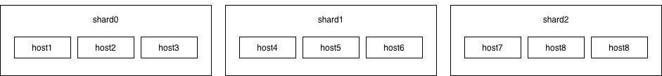
ClickHouse is linearly scalable; that is, the writes can be scaled by adding new shards and the reads can be scaled by adding new replicas. Every node in a ClickHouse cluster is identical. Not having any special nodes helps in scaling the cluster easily.

Let’s look at some optimizations we leveraged to provide faster read/write throughput and better compression on log data.

Inserter

Having an efficient inserter is as important as having an efficient data store. At Cloudflare, we have been operating quite a few analytics pipelines from where we borrowed most of the concepts while writing our new inserter. We use Cap’n Proto messages as the transport data format since it provides fast data encoding and decoding. Scaling inserters is easy and can be done by adding more Kafka partitions and spawning new inserter pods.

Batch Size

One of the key performance factors while inserting data into ClickHouse is the batch size. When batches are small, ClickHouse creates many small partitions, which it then merges into bigger ones. Thus smaller batch size creates extra work for ClickHouse to do in the background, thereby reducing ClickHouse’s performance. Hence it is crucial to set it big enough that ClickHouse can accept the data batch happily without hitting memory limits.

Data modeling in ClickHouse.

ClickHouse provides in-built sharding and replication without any external dependency. Earlier versions of ClickHouse depended on ZooKeeper for storing replication information, but the recent version removed the ZooKeeper dependency by adding clickhouse-keeper.

To read data across multiple shards, we use distributed tables, a special kind of table. These tables don’t store any data themselves but act as a proxy over multiple underlying tables storing the actual data.

Like any other database, choosing the right table schema is very important since it will directly impact the performance and storage utilization. We would like to discuss three ways you can store log data into ClickHouse.

The first is the simplest and the most strict table schema where you specify every column name and data type. Any logline having a field outside this predefined schema will get dropped. From our experience, this schema will give you the fastest query capabilities. If you already know the list of all possible fields ahead, we would recommend using it. You can always add or remove columns by running ALTER TABLE queries.

The second schema uses a very new feature of ClickHouse, where it does most of the heavy lifting. You can insert logs as JSON objects and behind the scenes, ClickHouse will understand your log schema and dynamically add new columns with appropriate data type and compression. This schema should only be used if you have good control over the log schema and the number of total fields is less than 1,000. On the one hand it provides flexibility to add new columns as new log fields automatically, but at the same time, one lousy application can easily bring down the ClickHouse cluster.

The third schema stores all fields of the same data type in one array and then uses ClickHouse inbuilt array functions to query those fields. This schema scales pretty well even when there are more than 1,000 fields, as the number of columns depends on the data types used in the logs. If an array element is accessed frequently, it can be taken out as a dedicated column using the materialized column feature of ClickHouse. We recommend adopting this schema since it provides safeguards against applications logging too many fields.

Data partitioning

A partition is a unit of ClickHouse data. One common mistake ClickHouse users make is overly granular partitioning keys, resulting in too many partitions. Since our logging pipeline generates TBs of data daily, we created the table partitioned with `toStartOfHour(dateTime).` With this partitioning logic, when a query comes with the timestamp in the WHERE clause, ClickHouse knows the partition and retrieves it quickly. It also helps design efficient data purging rules according to the data retention policies.

Primary key selection

ClickHouse stores the data on disk sorted by primary key. Thus, selecting the primary key impacts the query performance and helps in better data compression. Unlike relational databases, ClickHouse doesn’t require a unique primary key per row and we can insert multiple rows with identical primary keys. Having multiple primary keys will negatively impact the insertion performance. One of the significant ClickHouse limitations is that once a table is created the primary key can not be updated.

Data skipping indexes

ClickHouse query performance is directly proportional to whether it can use the primary key when evaluating the WHERE clause. We have many columns and all these columns can not be part of the primary key. Thus queries on these columns will have to do a full scan resulting in slower queries. In traditional databases, secondary indexes can be added to handle such situations. In ClickHouse, we can add another class of indexes called data skipping indexes, which uses bloom filters and skip reading significant chunks of data that are guaranteed to have no match.

ABR

We have multiple dashboards built over the requests_error logs. Loading these dashboards were often hitting the memory limits set for the individual query/user in ClickHouse.

The dashboards built over these logs were mainly used to identify anomalies. To visually identify an anomaly in a metric, the exact numbers are not required, but an approximate number would do. For instance, to understand that errors have increased in a data center, we don’t need the exact number of errors. So we decided to use an in-house library and tool built around a concept called ABR.

ABR stands for “Adaptive Bit Rate” – the term ABR is mainly used in video streaming services where servers select the best resolution for a video stream to match the client and network connection. It is described in great detail in the blog post – Explaining Cloudflare’s ABR Analytics

In other words, the data is stored at multiple resolutions or sample intervals and the best solution is picked for each query.

The way ABR works is at the time of writing requests to ClickHouse, it writes the data in a number of tables with different sample intervals. For instance table_1 stores 100% of data, table_10 stores 10% of data, table_100 stores 1% of data and table_1000 stores 0.1% data so on and so forth. The data is duplicated between the tables. Table_10 would be a subset of table_1.

Demo

In Cloudflare, we use in-house libraries and tools to insert data into ClickHouse, but this can be achieved by using an open source tool – vector.dev

If you would like to test how log ingestion into ClickHouse works, you can refer or use the demo here.

Make sure you have docker installed and run `docker compose up` to get started.

This would bring up three containers, Vector.dev for generating vector demo logs, writing it into ClickHouse, ClickHouse container to store the logs and Grafana instance to visualize the logs.

When the containers are up, visit http://localhost:3000/dashboards to play with the prebuilt demo dashboard.

Conclusion

Logs are supposed to be immutable by nature and ClickHouse works best with immutable data. We were able to migrate one of the critical and significant log-producing applications from Elasticsearch to a much smaller ClickHouse cluster.

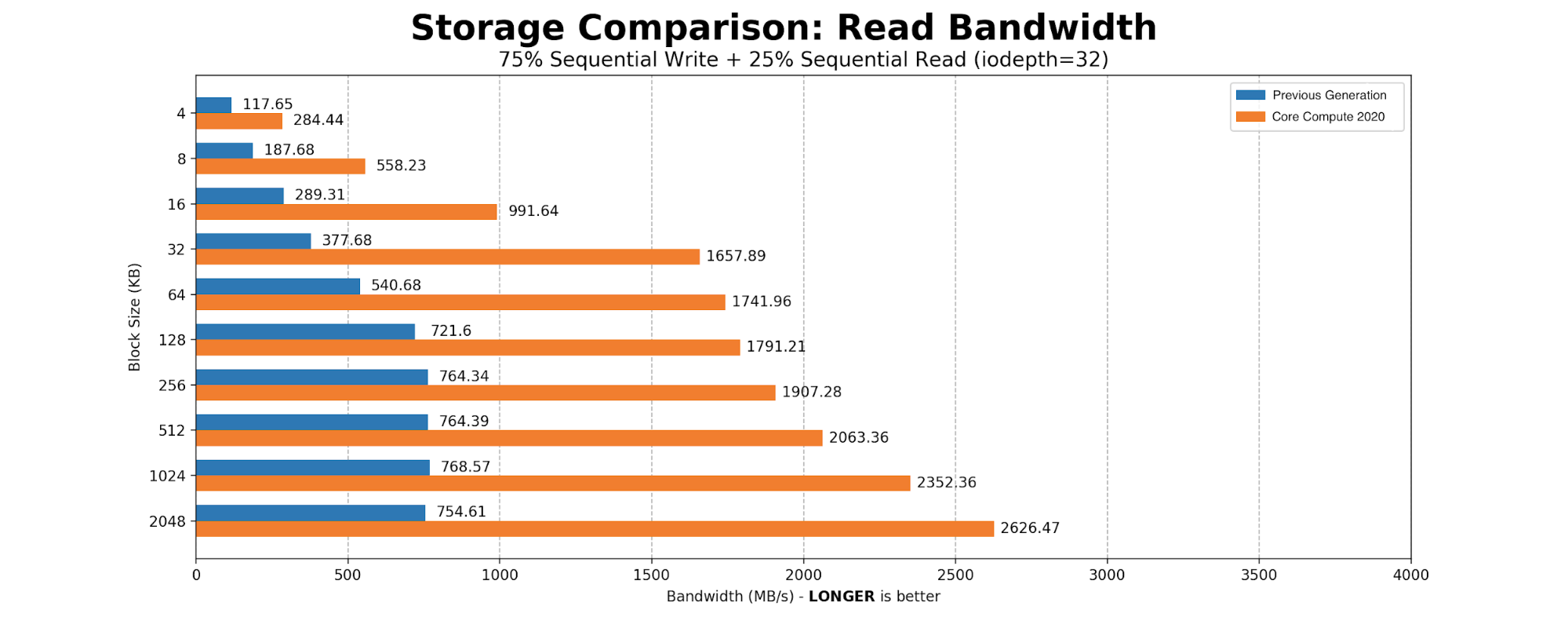
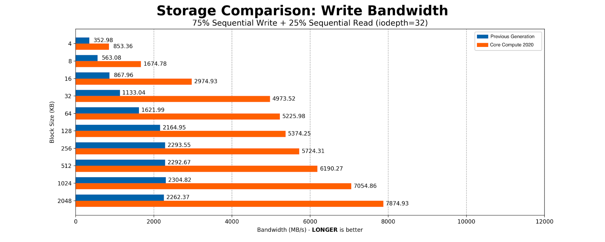
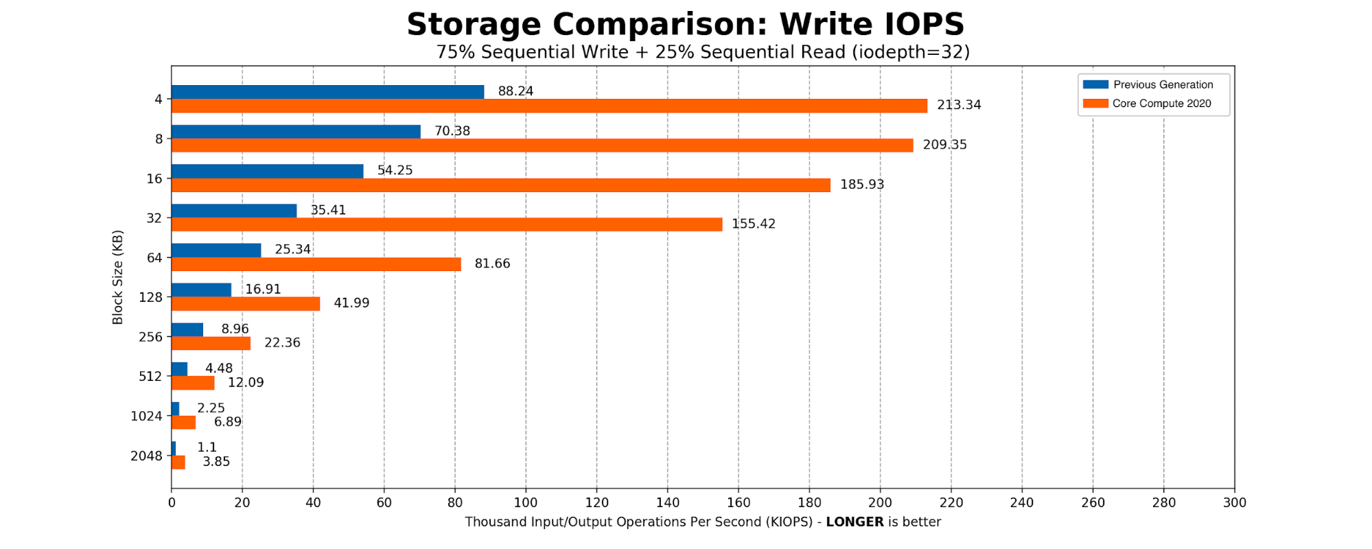
CPU and memory consumption on the inserter side were reduced by eight times. Each Elasticsearch document which used 600 bytes, came down to 60 bytes per row in ClickHouse. This storage gain allowed us to store 100% of the events in a newer setup. On the query side, the 99th percentile of the query latency also improved drastically.

Elasticsearch is great for full-text search and ClickHouse is great for analytics.

Getting to the Core: Benchmarking Cloudflare’s Latest Server Hardware

2020-11-20 Brian Bassett

Post Syndicated from Brian Bassett original https://blog.cloudflare.com/getting-to-the-core/

Getting to the Core: Benchmarking Cloudflare’s Latest Server Hardware

Maintaining a server fleet the size of Cloudflare’s is an operational challenge, to say the least. Anything we can do to lower complexity and improve efficiency has effects for our SRE (Site Reliability Engineer) and Data Center teams that can be felt throughout a server’s 4+ year lifespan.

At the Cloudflare Core, we process logs to analyze attacks and compute analytics. In 2020, our Core servers were in need of a refresh, so we decided to redesign the hardware to be more in line with our Gen X edge servers. We designed two major server variants for the core. The first is Core Compute 2020, an AMD-based server for analytics and general-purpose compute paired with solid-state storage drives. The second is Core Storage 2020, an Intel-based server with twelve spinning disks to run database workloads.

Core Compute 2020

Earlier this year, we blogged about our 10th generation edge servers or Gen X and the improvements they delivered to our edge in both performance and security. The new Core Compute 2020 server leverages many of our learnings from the edge server. The Core Compute servers run a variety of workloads including Kubernetes, Kafka, and various smaller services.

Configuration Changes (Kubernetes)

	Previous Generation Compute	Core Compute 2020
CPU	2 x Intel Xeon Gold 6262	1 x AMD EPYC 7642
Total Core / Thread Count	48C / 96T	48C / 96T
Base / Turbo Frequency	1.9 / 3.6 GHz	2.3 / 3.3 GHz
Memory	8 x 32GB DDR4-2666	8 x 32GB DDR4-2933
Storage	6 x 480GB SATA SSD	2 x 3.84TB NVMe SSD
Network	Mellanox CX4 Lx 2 x 25GbE	Mellanox CX4 Lx 2 x 25GbE

Configuration Changes (Kafka)

	Previous Generation (Kafka)	Core Compute 2020
CPU	2 x Intel Xeon Silver 4116	1 x AMD EPYC 7642
Total Core / Thread Count	24C / 48T	48C / 96T
Base / Turbo Frequency	2.1 / 3.0 GHz	2.3 / 3.3 GHz
Memory	6 x 32GB DDR4-2400	8 x 32GB DDR4-2933
Storage	12 x 1.92TB SATA SSD	10 x 3.84TB NVMe SSD
Network	Mellanox CX4 Lx 2 x 25GbE	Mellanox CX4 Lx 2 x 25GbE

Both previous generation servers were Intel-based platforms, with the Kubernetes server based on Xeon 6262 processors, and the Kafka server based on Xeon 4116 processors. One goal with these refreshed versions was to converge the configurations in order to simplify spare parts and firmware management across the fleet.

As the above tables show, the configurations have been converged with the only difference being the number of NVMe drives installed depending on the workload running on the host. In both cases we moved from a dual-socket configuration to a single-socket configuration, and the number of cores and threads per server either increased or stayed the same. In all cases, the base frequency of those cores was significantly improved. We also moved from SATA SSDs to NVMe SSDs.

Core Compute 2020 Synthetic Benchmarking

The heaviest user of the SSDs was determined to be Kafka. The majority of the time Kafka is sequentially writing 2MB blocks to the disk. We created a simple FIO script with 75% sequential write and 25% sequential read, scaling the block size from a standard page table entry size of 4096KB to Kafka’s write size of 2MB. The results aligned with what we expected from an NVMe-based drive.

Core Compute 2020 Production Benchmarking

Cloudflare runs many of our Core Compute services in Kubernetes containers, some of which are multi-core. By transitioning to a single socket, problems associated with dual sockets were eliminated, and we are guaranteed to have all cores allocated for any given container on the same socket.

Another heavy workload that is constantly running on Compute hosts is the Cloudflare CSAM Scanning Tool. Our Systems Engineering team isolated a Compute 2020 compute host and the previous generation compute host, had them run just this workload, and measured the time to compare the fuzzy hashes for images to the NCMEC hash lists and verify that they are a “miss”.

Because the CSAM Scanning Tool is very compute intensive we specifically isolated it to take a look at its performance with the new hardware. We’ve spent a great deal of effort on software optimization and improved algorithms for this tool but investing in faster, better hardware is also important.

In these heatmaps, the X axis represents time, and the Y axis represents “buckets” of time taken to verify that it is not a match to one of the NCMEC hash lists. For a given time slice in the heatmap, the red point is the bucket with the most times measured, the yellow point the second most, and the green points the least. The red points on the Compute 2020 graph are all in the 5 to 8 millisecond bucket, while the red points on the previous Gen heatmap are all in the 8 to 13 millisecond bucket, which shows that on average, the Compute 2020 host is verifying hashes significantly faster.

Core Storage 2020

Another major workload we identified was ClickHouse, which performs analytics over large datasets. The last time we upgraded our servers running ClickHouse was back in 2018.

Configuration Changes

	Previous Generation	Core Storage 2020
CPU	2 x Intel Xeon E5-2630 v4	1 x Intel Xeon Gold 6210U
Total Core / Thread Count	20C / 40T	20C / 40T
Base / Turbo Frequency	2.2 / 3.1 GHz	2.5 / 3.9 GHz
Memory	8 x 32GB DDR4-2400	8 x 32GB DDR4-2933
Storage	12 x 10TB 7200 RPM 3.5” SATA	12 x 10TB 7200 RPM 3.5” SATA
Network	Mellanox CX4 Lx 2 x 25GbE	Mellanox CX4 Lx 2 x 25GbE

CPU Changes

For ClickHouse, we use a 1U chassis with 12 x 10TB 3.5” hard drives. At the time we were designing Core Storage 2020 our server vendor did not yet have an AMD version of this chassis, so we remained on Intel. However, we moved Core Storage 2020 to a single 20 core / 40 thread Xeon processor, rather than the previous generation’s dual-socket 10 core / 20 thread processors. By moving to the single-socket Xeon 6210U processor, we were able to keep the same core count, but gained 17% higher base frequency and 26% higher max turbo frequency. Meanwhile, the total CPU thermal design profile (TDP), which is an approximation of the maximum power the CPU can draw, went down from 165W to 150W.

On a dual-socket server, remote memory accesses, which are memory accesses by a process on socket 0 to memory attached to socket 1, incur a latency penalty, as seen in this table:

	Previous Generation	Core Storage 2020
Memory latency, socket 0 to socket 0	81.3 ns	86.9 ns
Memory latency, socket 0 to socket 1	142.6 ns	N/A

An additional advantage of having a CPU with all 20 cores on the same socket is the elimination of these remote memory accesses, which take 76% longer than local memory accesses.

Memory Changes

The memory in the Core Storage 2020 host is rated for operation at 2933 MHz; however, in the 8 x 32GB configuration we need on these hosts, the Intel Xeon 6210U processor clocks them at 2666 MH. Compared to the previous generation, this gives us a 13% boost in memory speed. While we would get a slightly higher clock speed with a balanced, 6 DIMMs configuration, we determined that we are willing to sacrifice the slightly higher clock speed in order to have the additional RAM capacity provided by the 8 x 32GB configuration.

Storage Changes

Data capacity stayed the same, with 12 x 10TB SATA drives in RAID 0 configuration for best throughput. Unlike the previous generation, the drives in the Core Storage 2020 host are helium filled. Helium produces less drag than air, resulting in potentially lower latency.

Core Storage 2020 Synthetic benchmarking

We performed synthetic four corners benchmarking: IOPS measurements of random reads and writes using 4k block size, and bandwidth measurements of sequential reads and writes using 128k block size. We used the fio tool to see what improvements we would get in a lab environment. The results show a 10% latency improvement and 11% IOPS improvement in random read performance. Random write testing shows 38% lower latency and 60% higher IOPS. Write throughput is improved by 23%, and read throughput is improved by a whopping 90%.

	Previous Generation	Core Storage 2020	% Improvement
4k Random Reads (IOPS)	3,384	3,758	11.0%
4k Random Read Mean Latency (ms, lower is better)	75.4	67.8	10.1% lower
4k Random Writes (IOPS)	4,009	6,397	59.6%
4k Random Write Mean Latency (ms, lower is better)	63.5	39.7	37.5% lower
128k Sequential Reads (MB/s)	1,155	2,195	90.0%
128k Sequential Writes (MB/s)	1,265	1,558	23.2%

CPU frequencies

The higher base and turbo frequencies of the Core Storage 2020 host’s Xeon 6210U processor allowed that processor to achieve higher average frequencies while running our production ClickHouse workload. A recent snapshot of two production hosts showed the Core Storage 2020 host being able to sustain an average of 31% higher CPU frequency while running ClickHouse.

	Previous generation (average core frequency)	Core Storage 2020 (average core frequency)	% improvement
Mean Core Frequency	2441 MHz	3199 MHz	31%

Core Storage 2020 Production benchmarking

Our ClickHouse database hosts are continually performing merge operations to optimize the database data structures. Each individual merge operation takes just a few seconds on average, but since they’re constantly running, they can consume significant resources on the host. We sampled the average merge time every five minutes over seven days, and then sampled the data to find the average, minimum, and maximum merge times reported by a Compute 2020 host and by a previous generation host. Results are summarized below.

ClickHouse merge operation performance improvement
(time in seconds, lower is better)

Time	Previous generation	Core Storage 2020	% improvement
Mean time to merge	1.83	1.15	37% lower
Maximum merge time	3.51	2.35	33% lower
Minimum merge time	0.68	0.32	53% lower

Our lab-measured CPU frequency and storage performance improvements on Core Storage 2020 have translated into significantly reduced times to perform this database operation.

Conclusion

With our Core 2020 servers, we were able to realize significant performance improvements, both in synthetic benchmarking outside production and in the production workloads we tested. This will allow Cloudflare to run the same workloads on fewer servers, saving CapEx costs and data center rack space. The similarity of the configuration of the Kubernetes and Kafka hosts should help with fleet management and spare parts management. For our next redesign, we will try to further converge the designs on which we run the major Core workloads to further improve efficiency.

Special thanks to Will Buckner and Chris Snook for their help in the development of these servers, and to Tim Bart for validating CSAM Scanning Tool’s performance on Compute.

ClickHouse Capacity Estimation Framework

2020-11-05 Oxana Kharitonova

Post Syndicated from Oxana Kharitonova original https://blog.cloudflare.com/clickhouse-capacity-estimation-framework/

ClickHouse Capacity Estimation Framework

We use ClickHouse widely at Cloudflare. It helps us with our internal analytics workload, bot management, customer dashboards, and many other systems. For instance, before Bot Management can analyze and classify our traffic, we need to collect logs. The Firewall Analytics tool needs to store and query data somewhere too. The same goes for our new Cloudflare Radar project. We are using ClickHouse for this purpose. It is a big database that can store huge amounts of data and return it on demand. This is not the first time we have talked about ClickHouse, there is a dedicated blogpost on how we introduced ClickHouse for HTTP analytics.

Our biggest cluster has more than 100 nodes, another one about half that number. Besides that, we have over 20 clusters that have at least three nodes and the replication factor of three. Our current insertion rate is about 90M rows per second.

We use the standard approach in ClickHouse schema design. At the top level we have clusters, which hold shards, a group of nodes, and a node is a physical machine. You can find technical characteristics of the nodes here. Stored data is replicated between clusters. Different shards hold different parts of the data, but inside of each shard replicas are equal.

Schema of one cluster:

ClickHouse Capacity Estimation Framework

Capacity planning

As engineers, we periodically face the question of how many additional nodes we have to order to support the growing demand for the next X months, with disk space as our prime concern.

ClickHouse stores extensive information in system tables about the operating processes, which is helpful. From the early days of using ClickHouse we added clickhouse_exporter as part of our monitoring stack. One of the metrics we are interested in is exposed from the system.parts table. Roughly speaking, clickhouse_exporter runs SQL queries asking how many bytes are used by each table. After that, these metrics are sent from Prometheus to Thanos and stored for at least a year.

Every time we wanted to make a forecast of disk usage we queried Thanos for historical data using this expression:

sum by (table) (sum(table_parts_bytes{cluster="{cluster}"}))

After that, we uploaded data in dataframes to a Jupyter notebook.

There were a few problems with this approach. Only a few people knew where the notebooks were and how to get them running. It wasn’t trivial to download historical data. And most importantly, it was hard to look at past predictions and assess whether or not they were correct since results were not stored anywhere except internal blog posts. Also, as the number and size of clusters and products grew it became impossible for a single team to work on capacity planning and we needed to get engineers building products involved as they have the most context on how the growth will change in the future.

We wanted to automate this process and made calculations more transparent for our colleagues, including those who use ClickHouse for their services. Honestly, at the beginning we weren’t sure if it was even possible and what we would get out of it.

Finding the right metrics

The crucial moment of adding new nodes for us is a disk space, so this was a place to start. We decided to use system.parts, as we used it before with the manual approach.

Luckily, we started doing it for the cluster that had recently changed its topology. That cluster had two shards with four and five nodes in every shard. After the topology change, it was replaced with three shards and three nodes in every shard, but the number of machines and unreplicated data on the disks remained the same. However, it had an impact on our metrics: we previously had four replicated nodes in one shard and five replicated in another, we took one node off from the first shard and two nodes from the second and created a new one based on these three nodes. The new shard was empty, so we just added it, but the total amount of data in the first and the second shards was less as the count of the remaining nodes.

You can see on the graph below in April we had this sharp decrease caused by topology changes. We got ~550T instead of ~850T among all shards and replicas.

When we tried to train our model based on the real data due to the April drop it thought we had a downward trend. Which was incorrect as we only dropped replicated data. The trend for unreplicated data hadn’t changed. So we decided to take into account only unreplicated data. It saved us from the topology change and node replacement in case of problems with hardware.

The rule that we use for metrics now is:

sum by(cluster) (
max by (cluster, shardgroup) (
node_clickhouse_shardgroupinfo{} *
on (instance) group_right (cluster, shardgroup) sum(table_parts_bytes{cluster="%s"}) by (instance)
))

We continue using system.parts from clickhouse_exporter, but instead of counting the whole amount of data we use the maximum of unreplicated data from every shard.

In the image below there is the same cluster as in the image above but instead of counting the whole amount of data we look at unreplicated data from all shards. You can clearly see that we continued to grow and didn’t have any drop in data.

Another problem we faced was that we migrated some tables from one cluster to another because we were running out of space and it required immediate action. However, our model didn’t know that part of the tables didn’t live there anymore, and we didn’t want them to be a part of the prediction. To solve this problem we queried Prometheus to get the list of the tables that existed at the prediction time, then filtered historical data to include only these tables and used them as the input for training a model.

Load of metrics

After determining the correct metrics, we needed to obtain them for our forecasting procedure. Our long-term metrics solution, Thanos, stores billions of data points. Querying it for a cluster with over one hundred nodes even for one day takes a huge amount of time, and we needed these data points for a year.

As we planned to use Python we wrote a small client using aiohttp that concurrently sends HTTP requests to Thanos. The requests are sent in chunks, and every request has start/end dates with a difference of one hour. We needed to get the data for the whole year once and then append new ones day by day. We got csv files: one file for one cluster. The client became a part of the project, and it runs once a day, queries Thanos for new metrics (previous day) and appends data to the files.

Forecasting procedure

At this point, we have collected metrics in files, now it’s time to make a forecast. We needed something for time-series metrics, so we chose Prophet from Facebook. It’s very simple to use, you can follow the documentation and get good results even with the default parameters.

One challenge we faced using Prophet was the need to feed it one data point for a day. In the metric files we have thousands of those for every day. It looks logical to take the point at the end of every day, but it’s not really true. All tables have a retention period, the time for how long we store data in ClickHouse. We don’t know when the data is cleared, it happens gradually throughout the day. So, we decided to take the maximum number for a day.

Drawing Graphs

We chose Grafana to present results, though we needed to store predicted data points somewhere. The first thought was to use Prometheus, but because of high cardinality, we had about 300,000 points in summary for clusters and tables, so we passed. We decided to use ClickHouse itself. We wanted to have both graphs, real and predicted, on the same dashboard. We had real data points in Prometheus and with mixed data source could do this. However, the problem was the same as the loading of metrics into files, for some clusters it’s impossible to obtain metrics for a long period of time. We added functionality to upload real metrics in ClickHouse as well, now both real and predicted metrics are displayed in Grafana, taken from ClickHouse.

Summary

This is what we have in Grafana:

The yellow line shows the real data;
The green line was created based on Prophet output;
The red line – the maximum disk capacity. We already increased it twice.

We have a service running in Kubernetes that does all the toil, and we created an environment for other metrics. We have the place where we collect metrics from Thanos and expose them in the required format to Grafana. If we find the right metrics for accounting other resources like IO, CPU or other systems like Kafka we can easily add them to our framework. We can easily replace Prophet with another algorithm, and we can go back months and evaluate how close we were in our prediction according to the real data.

With this automation we were able to spot we were going out of disk space for a couple of clusters which we didn’t expect. We have over 20 clusters and have updates for all of them every day. This dashboard is used not only by our colleagues who are direct customers of ClickHouse but by the team who makes a plan for buying servers. It is easy to read and costs none of developers time.

This project was carried out by the Core SRE team to improve our daily work. If you are interested in this project, check out our job openings.

We didn’t know what we would get at the end, we discussed, looked for solutions and tried different approaches. Huge thanks for this to Nicolae Vartolomei, Alex Semiglazov and John Skopis.

Characteristics of logs

Logging pipeline

Elasticsearch bottlenecks at Cloudflare

Mapping Explosion

Multi-tenancy support

Cluster operational tasks

Garbage collection

Proposed solution

Inserter

Batch Size

Data modeling in ClickHouse.

Data partitioning

Primary key selection

Data skipping indexes

ABR

Demo

Conclusion

Core Compute 2020

Configuration Changes (Kubernetes)

Core Compute 2020 Synthetic Benchmarking

Core Compute 2020 Production Benchmarking

Core Storage 2020

Configuration Changes

Memory Changes

Storage Changes

Core Storage 2020 Synthetic benchmarking

CPU frequencies

Core Storage 2020 Production benchmarking

ClickHouse merge operation performance improvement(time in seconds, lower is better)

Conclusion

Capacity planning

Finding the right metrics

Load of metrics

Forecasting procedure

Drawing Graphs

Summary

The collective thoughts of the interwebz

ClickHouse merge operation performance improvement
(time in seconds, lower is better)