Tag Archives: observability

Announcing Workers automatic tracing, now in open beta

Post Syndicated from Nevi Shah original https://blog.cloudflare.com/workers-tracing-now-in-open-beta/

When your Worker slows down or starts throwing errors, finding the root cause shouldn’t require hours of log analysis and trial-and-error debugging. You should have clear visibility into what’s happening at every step of your application’s request flow. This is feedback we’ve heard loud and clear from developers using Workers, and today we’re excited to announce an Open Beta for tracing on Cloudflare Workers! You can now:  

  • Get automatic instrumentation for applications on the Workers platform: No manual setup, complex instrumentation, or code changes. It works out of the box. 

  • Explore and investigate traces in the Cloudflare dashboard: Your traces are processed and available in the Workers Observability dashboard alongside your existing logs.

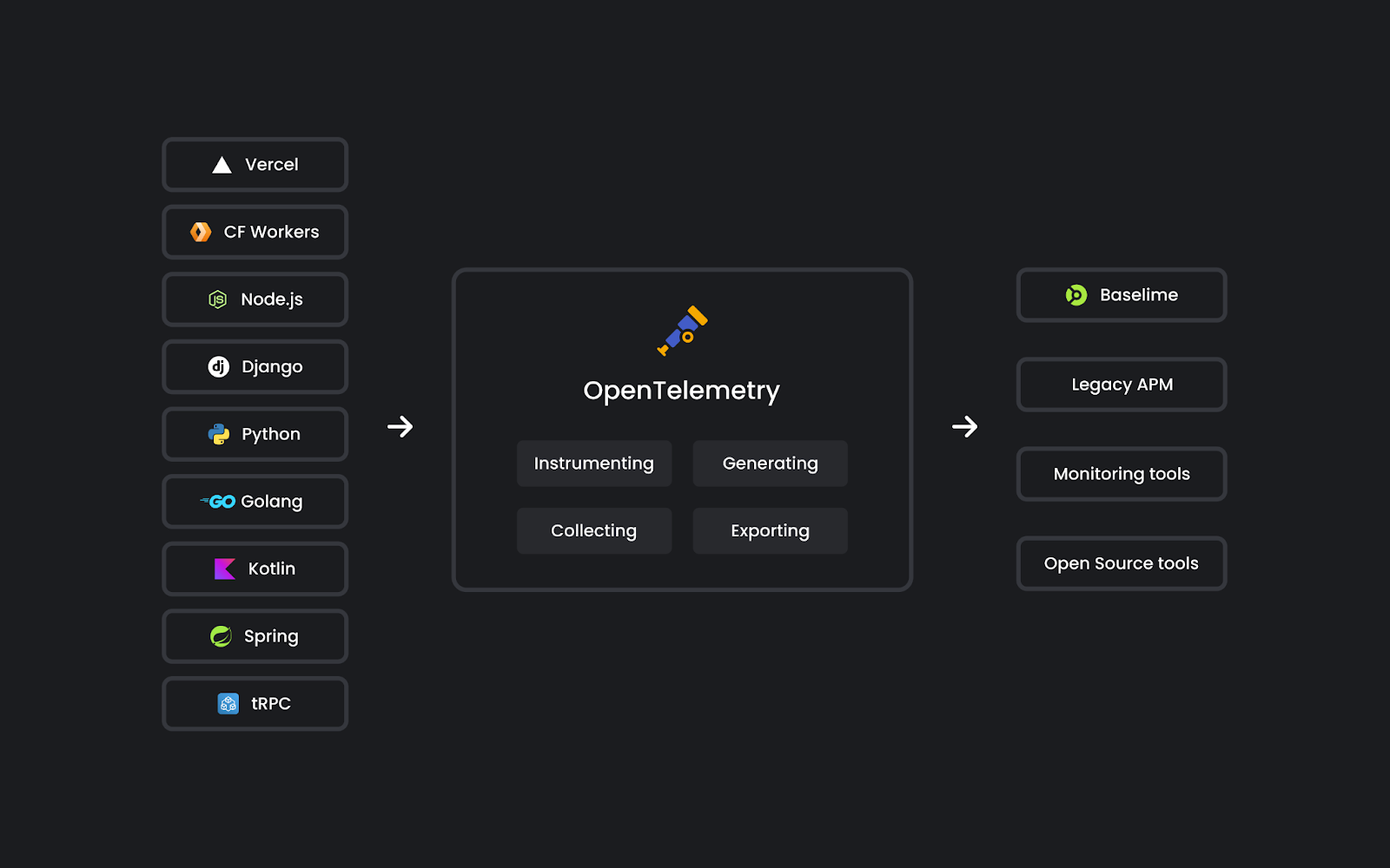
  • Export logs and traces to OpenTelemetry-compatible providers: Send OpenTelemetry traces (and correlated logs) to your observability provider of choice. 

In 2024, we set out to build the best first-party observability of any cloud platform. We launched a new metrics dashboard to give better insights into how your Worker is performing, Workers Logs to automatically ingest and store logs for your Workers, a query builder to explore your data across any dimension and real-time logs to stream your logs in real time with advanced filtering capabilities. Starting today, you can get an even deeper understanding of your Workers applications by enabling automatic tracing!

What is Workers Tracing? 

Workers traces capture and emit OpenTelemetry-compliant spans to show you detailed metadata and timing information on every operation your Worker performs. It helps you identify performance bottlenecks, resolve errors, and understand how your Worker interacts with other services on the Workers platform. You can now answer questions like:

  • Which calls are slowing down my application?

  • Which queries to my database take the longest? 

  • What happened within a request that resulted in an error?

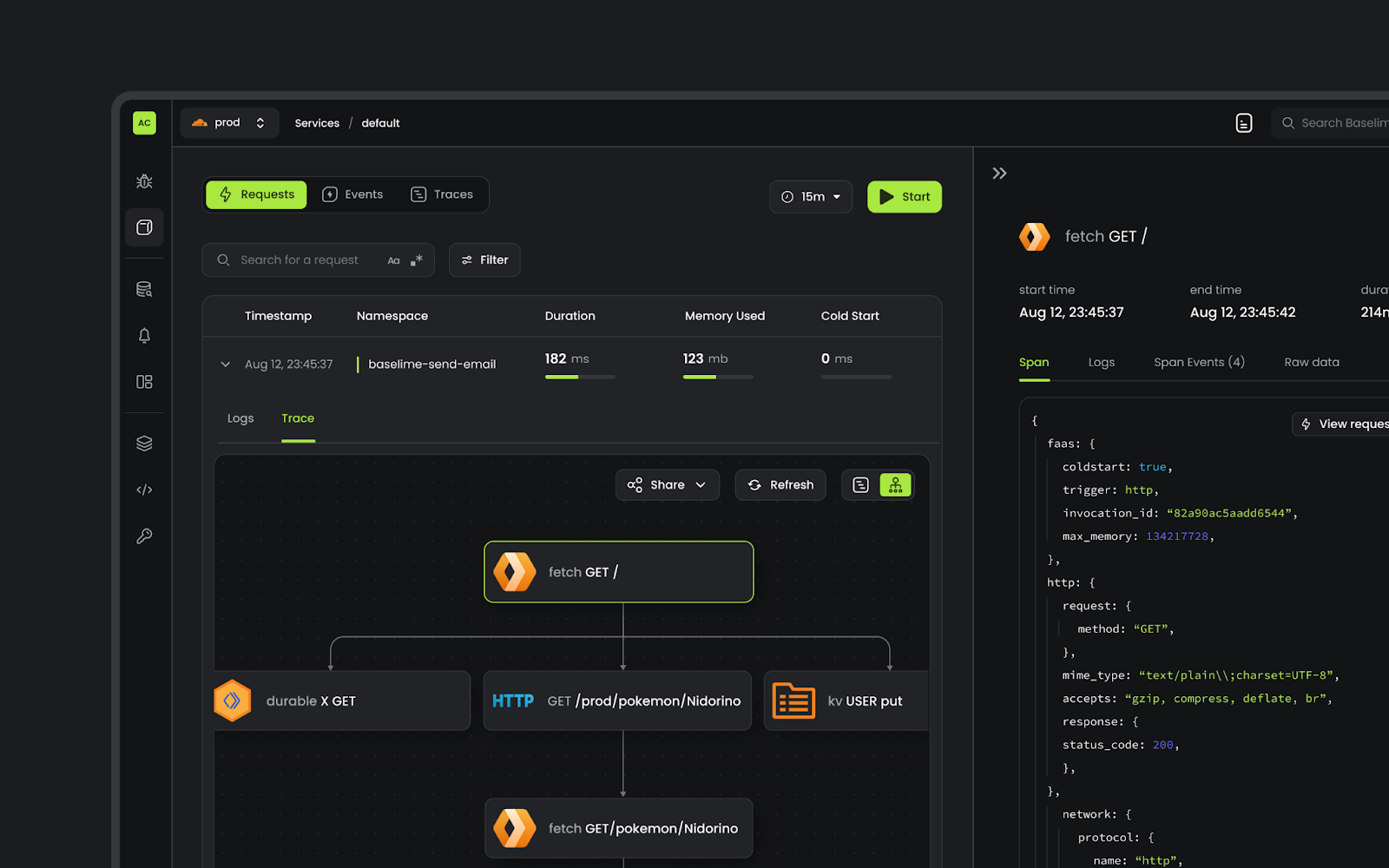
Tracing provides a visualization of each invocation’s journey through various operations. Each operation is captured as a span, a timed segment that shows what happened and how long it took. Child spans nest within parent spans to show sub-operations and dependencies, creating a hierarchical view of your invocation’s execution flow. Each span can include contextual metadata or attributes that provide details for debugging and filtering events.


Full automatic instrumentation, no code changes 

Previously, instrumenting your application typically required an understanding of the OpenTelemetry spec, multiple OTel libraries, and how they related to each other. Implementation was tedious and bloated your codebase with instrumentation code that obfuscated your application logic.

Setting up tracing typically meant spending hours integrating third-party SDKs, wrapping every database call and API request with instrumentation code, and debugging complex config files before you saw a single trace. This implementation overhead often makes observability an afterthought, leaving you without full visibility in production when issues arise.

What makes Workers Tracing truly magical is it’s completely automatic – no set up, no code changes, no wasted time. We took the approach of automatically instrumenting every I/O operation in your Workers, through a deep integration in workerd, our runtime, enabling us to capture the full extent of data flows through every invocation of your Workers.

You focus on your application logic. We take care of the instrumentation.

What you can trace today

The operations covered today are: 

  • Binding calls: Interactions with various Worker bindings. KV reads and writes, R2 object storage operations, Durable Object invocations, and many more binding calls are automatically traced. This gives you complete visibility into how your Worker uses other services.

  • Fetch calls: All outbound HTTP requests are automatically instrumented, capturing timing, status codes, and request metadata. This enables you to quickly identify which external dependencies are affecting your application’s performance.

  • Handler calls: Methods on a Worker that can receive and process external inputs, such as fetch handlers, scheduled handlers, and queue handlers. This gives you visibility into performance of how your Worker is being invoked.

Automatic attributes on every span 

Our automated instrumentation captures each operation as a span. For example, a span generated by an R2 binding call (like a get or put operation) will automatically contain any available attributes, such as the operation type, the error if applicable, the object key, and duration. These detailed attributes provide the context you need to answer precise questions about your application without needing to manually log every detail.


We will continue to add more detailed attributes to spans and add the ability to trace an invocation across multiple Workers or external services. Our documentation contains a complete list of all instrumented spans and their attributes.

Investigate traces in the Workers dashboard

You can easily view traces directly within a specific Worker application in the Cloudflare dashboard, giving you immediate visibility into your application’s performance. You’ll find a list of all trace events within your desired time frame and a trace visualization of each invocation including duration of each call and any available attributes. You can also query across all Workers on your account, letting you pinpoint issues occurring on multiple applications.


To get started viewing traces on your Workers application, you can set: 


Or if you already have observability.enabled=true configured, traces will be automatically emitted alongside your logs.


Export traces to OpenTelemetry compatible providers 

However, we realize that some development teams need Workers data to live alongside other telemetry data in the tools they are already using. That’s why we’re also adding tracing exports, letting your team send, visualize and query data with your existing observability stack! Starting today, you can export traces directly to providers like Honeycomb, Grafana or any other OpenTelemetry Protocol (OTLP) provider with an available endpoint.


Correlated logs and traces 

We also support exporting OTLP-formatted logs that share the same trace ID, enabling third-party platforms to automatically correlate log entries with their corresponding traces. This lets you easily jump between spans and related log messages.

Set up your destination, enable exports, and go! 

To start sending events to your destination of choice, first, configure your OTLP endpoint destination in the Cloudflare dashboard. For every destination you can specify a custom name and set custom headers to include API keys or app configuration. 

Once you have your destination set up (e.g. honeycomb-tracing), set the following in your wrangler.jsonc and deploy: 


Coming up for Workers observability

This is just the beginning of Workers providing the workflows and tools to get you the telemetry data you want, where you want it. We’re improving our support both for native tracing in the dashboard and for exporting other types of telemetry to 3rd parties. In the upcoming months we’ll be launching: 

  • Support for more spans and attributes: We are adding more automatic traces for every part of the Workers platform. While our first goal is to give you visibility into the duration of every operation within your request, we also want to add detailed attributes. Your feedback on what’s missing will be extremely valuable here. 

  • Trace context propagation: When building distributed applications, ensuring your traces connect across all of your services (even those outside of Cloudflare), automatically linking spans together to create complete, end-to-end visibility is critical. For example, a trace from Workers could be nested from a parent service or vice versa. When fully implemented, our automatic trace context propagation will follow W3C standards to ensure compatibility across your existing tools and services. 

  • Support for custom spans and attributes: While automatic instrumentation gives you visibility into what’s happening within the Workers platform, we know you need visibility into your own application logic too. So, we’ll give you the ability to manually add your own spans as well.

  • Ability to export metrics: Today, metrics, logs and traces are available for you to monitor and view within the Workers dashboard. But the final missing piece is giving you the ability to export both infrastructure metrics (like request volume, error rates, and execution duration) and custom application metrics to your preferred observability provider.

What you can expect from tracing pricing  

Today, at the start of beta, viewing traces in the Cloudflare dashboard and exporting traces to a 3rd party provider are both free. On January 15, 2026, tracing and log events will be charged the following pricing:

Viewing Workers traces in the Cloudflare dashboard

To view traces in the Cloudflare dashboard, you can do so on a Workers Free and Paid plan at the pricing shown below:

Workers Free Workers Paid
Included Volume 200K events per day 20M events per month
Additional Events N/A $0.60 per million logs
Retention 3 days 7 days

Exporting traces and logs 

To export traces to a 3rd-party OTLP-compatible destination, you will need a Workers Paid subscription. Pricing is based on total span or log events with the following inclusions:

Workers Free Workers Paid
Events Not available 10 million events per month
Additional events $0.05 per million batched events

Enable tracing today

Ready to get started with tracing on your Workers application? 

  • Check out our documentation: Learn how to get set up, read about current limitations and discover more about what’s coming up. 

  • Join the chatter in our GitHub discussion: Your feedback will be extremely valuable in our beta period on our automatic instrumentation, tracing dashboard, and OpenTelemetry export flow. Head to our GitHub discussion to raise issues, put in feature requests and get in touch with us!

Performance measurements… and the people who love them

Post Syndicated from Kevin Guthrie original https://blog.cloudflare.com/loving-performance-measurements/

⚠️ WARNING ⚠️ This blog post contains graphic depictions of probability. Reader discretion is advised.

Measuring performance is tricky. You have to think about accuracy and precision. Are your sampling rates high enough? Could they be too high?? How much metadata does each recording need??? Even after all that, all you have is raw data. Eventually for all this raw performance information to be useful, it has to be aggregated and communicated. Whether it’s in the form of a dashboard, customer report, or a paged alert, performance measurements are only useful if someone can see and understand them.

This post is a collection of things I’ve learned working on customer performance escalations within Cloudflare and analyzing existing tools (both internal and commercial) that we use when evaluating our own performance.  A lot of this information also comes from Gil Tene’s talk, How NOT to Measure Latency. You should definitely watch that too (but maybe after reading this, so you don’t spoil the ending). I was surprised by my own blind spots and which assumptions turned out to be wrong, even though they seemed “obviously true” at the start. I expect I am not alone in these regards. For that reason this journey starts by establishing fundamental definitions and ends with some new tools and techniques that we will be sharing as well as the surprising results that those tools uncovered.

Check your verbiage

So … what is performance? Alright, let’s start with something easy: definitions. “Performance” is not a very precise term because it gets used in too many contexts. Most of us as nerds and engineers have a gut understanding of what it means, without a real definition. We can’t really measure it because how “good” something is depends on what makes that thing good. “Latency” is better … but not as much as you might think. Latency does at least have an implicit time unit, so we can measure it. But … what is latency? There are lots of good, specific examples of measurements of latency, but we are going to use a general definition. Someone starts something, and then it finishes — the elapsed time between is the latency.


This seems a bit reductive, but it’s a surprisingly useful definition because it gives us a key insight. This fundamental definition of latency is based around the client’s perspective. Indeed, when we look at our internal measurements of latency for health checks and monitoring, they all have this one-sided caller/callee relationship. There is the latency of the caching layer from the point of view of the ingress proxy. There’s the latency of the origin from the cache’s point of view. Each component can measure the latency of its upstream counterparts, but not the other way around. 

This one-sided nature of latency observation is a real problem for us because Cloudflare only exists on the server side. This makes all of our internal measurements of latency purely estimations. Even if we did have full visibility into a client’s request timing, the start-to-finish latency of a request to Cloudflare isn’t a great measure of Cloudflare’s latency. The process of making an HTTP request has lots of steps, only a subset of which are affected by us. Time spent on things like DNS lookup, local computation for TLS, or resource contention do affect the client’s experience of latency, but only serve as sources of noise when we are considering our own performance.

There is a very useful and common metric that is used to measure web requests, and I’m sure lots of you have been screaming it in your brains from the second you read the title of this post. ✨Time to first byte✨. Clearly this is the answer, right?!  But … what is “Time to first byte”?

TTFB mine

Time to first byte (TTFB) on its face is simple. The name implies that it’s the time it takes (on the client’s side) to receive the first byte of the response from the server, but unfortunately, that only describes when the timer should end. It doesn’t say when the timer should start. This ambiguity is just one factor that leads to inconsistencies when trying to compare TTFB across different measurement platforms … or even across a single platform because there is no one definition of TTFB. Similar to “performance”, it is used in too many places to have a single definition. That being said, TTFB is a very useful concept, so in order to measure it and report it in an unambiguous way, we need to pick a definition that’s already in use.

We have mentioned TTFB in other blog posts, but this one sums up the problem best with “Time to first byte isn’t what it used to be.” You should read that article too, but the gist is that one popular TTFB definition used by browsers was changed in a confusing way with the introduction of early hints in June 2022. That post and others make the point that while TTFB is useful, it isn’t the best direct measurement for web performance. Later on in this post we will derive why that’s the case.

One common place we see TTFB used is our customers’ analysis comparing Cloudflare’s performance to our competitors through Catchpoint. Customers, as you might imagine, have a vested interest in measuring our latency, as it affects theirs. Catchpoint provides several tools built on their global Internet probe network for measuring HTTP request latency (among other things) and visualizing it in their web interface. In an effort to align better with our customers, we decided to adopt Catchpoint’s terminology for talking about latency, both internally and externally.

Catchpoint catch-up

While Catchpoint makes things like TTFB easy to plot over time, the visualization tool doesn’t give a definition of what TTFB is, but after going through all of their technical blog posts and combing through thousands of lines of raw data, we were able to get functional definitions for TTFB and other composite metrics. This was an important step because these metrics are how our customers are viewing our performance, so we all need to be able to understand exactly what they signify! The final report for this is internal (and long and dry), so in this post, I’ll give you the highlights in the form of colorful diagrams, starting with this one.


This diagram shows our customers’ most commonly viewed client metrics on Catchpoint and how they fit together into the processing of a request from the server side. Notice that some are directly measured, and some are calculated based on the direct measurements. Right in the middle is TTFB, which Catchpoint calculates as the sum of the DNS, Connect, TLS, and Wait times. It’s worth noting again that this is not the definition of TTFB, this is just Catchpoint’s definition, and now ours.

This breakdown of HTTPS phases is not the only one commonly used. Browsers themselves have a standard for measuring the stages of a request. The diagram below shows how most browsers are reporting request metrics. Luckily (and maybe unsurprisingly) these phases match Catchpoint’s very closely.


There are some differences beyond the inclusion of things like AppCache and Redirects (which are not directly impacted by Cloudflare’s latency). Browser timing metrics are based on timestamps instead of durations. The diagram subtly calls this out with gaps between the different phases indicating that there is the potential for the computer running the browser to do things that are not part of any phase. We can line up these timestamps with Catchpoint’s metrics like so:


Now that we, our customers, and our browsers (with data coming from RUM) have a common and well-defined language to talk about the phases of a request, we can start to measure, visualize, and compare the components that make up the network latency of a request. 

Visual basics

Now that we have defined what our key values for latency are, we can record numbers and put them in a chart and watch them roll by … except not directly. In most cases, the systems we use to record the data actively prevent us from seeing the recorded data in its raw form. Tools like Prometheus are designed to collect pre-aggregated data, not individual samples, and for a good reason. Storing every recorded metric (even compacted) would be an enormous amount of data. Even worse, the data loses its value exponentially over time, since the most recent data is the most actionable.

The unavoidable conclusion is that some aggregation has to be done before performance data can be visualized. In most cases, the aggregation means looking at a series of windowed percentiles over time. The most common are 50th percentile (median), 75th, 90th, and 99th if you’re really lucky. Here is an example of a latency visualization from one of our own internal dashboards.


It clearly shows a spike in latency around 14:40 UTC. Was it an incident? The p99 jumped by 1300% (500ms to 6500

ms) for multiple minutes while the p50 jumped by more than 13600% (4.4ms to 600ms). It is a clear signal, so something must have happened, but what was it? Let me keep you in suspense for a second while we talk about statistics and probability.

Uncooked math

Let me start with a quote from my dear, close, personal friend @ThePrimeagen:


It’s a good reminder that while statistics is a great tool for providing a simplified and generalized representation of a complex system, it can also obscure important subtleties of that system. A good way to think of statistical modeling is like lossy compression. In the latency visualization above (which is a plot of TTFB over time), we are compressing the entire spectrum of latency metrics into 4 percentile bands, and because we are only considering up to the 99th percentile, there’s an entire 1% of samples left over that we are ignoring! 

“What?” I hear you asking. “P99 is already well into perfection territory. We’re not trying to be perfectionists. Maybe we should get our p50s down first”. Let’s put things in perspective. This zone (www.cloudflare.com) is getting about 30,000 req/s and the 99th percentile latency is 500 ms. (Here we are defining latency as “Edge TTFB”, a server-side approximation of our now official definition.) So there are 300 req/s that are taking longer than half a second to complete, and that’s just the portion of the request that we can see. How much worse than 500 ms are those requests in the top 1%? If we look at the 100th percentile (the max), we get a much different vibe from our Edge TTFB plot.


Viewed like this, the spike in latency no longer looks so remarkable. Without seeing more of the picture, we could easily believe something was wrong when in reality, even if something is wrong, it is not localized to that moment. In this case, it’s like we are using our own statistics to lie to ourselves. 

The top 1% of requests have 99% of the latency

Maybe you’re still not convinced. It feels more intuitive to focus on the median because the latency experienced by 50 out of 100 people seems more important to focus on than that of 1 in 100. I would argue that is a totally true statement, but notice I said “people” and not “requests.” A person visiting a website is not likely to be doing it one request at a time.

Taking www.cloudflare.com as an example again, when a user opens that page, their browser makes more than 70 requests. It sounds big, but in the world of user-facing websites, it’s not that bad. In contrast, www.amazon.com issues more than 400 requests! It’s worth noting that not all those requests need to complete before a web page or application becomes usable. That’s why more advanced and browser-focused metrics exist, but I will leave a discussion of those for later blog posts. I am more interested in how making that many requests changes the probability calculations for expected latency on a per-user basis. 

Here’s a brief primer on combining probabilities that covers everything you need to know to understand this section.

  • The probability of two things happening is the probability of the first happening multiplied by the probability of the second thing happening. $$P(X\cap Y )=P(X) \times P (Y)$$

  • The probability of something in the $X^{th}$ percentile happening is $X\%$. $$P(pX) = X\%$$

Let’s define $P( pX_{N} )$ as the probability that someone on a website with $N$ requests experiences no latencies >= the $X^{th}$ percentile. For example, $P(p50_{2})$ would be the probability of getting no latencies greater than the median on a page with 2 requests. This is equivalent to the probability of one request having a latency less than the $p50$ and the other request having a latency less than the $p50$. We can use the first identities above. 

$$\begin{align}
P( p50_{2}) &= P\left ( p50 \cap p50 \right ) \\
  &= P( p50) \times P\left ( p50 \right ) \\
  &= 50\%^{2} \\
  &= 25\%
\end{align}$$

We can generalize this for any percentile and any number of requests. $$P( pX_{N}) = X\%^{N}$$

For www.cloudflare.com and its 70ish requests, the percentage of visitors that won’t experience a latency above the median is 

$$\begin{align}
P( p50_{70}) &= 50\%^{70} \\
  &\approx 0.000000000000000000001\%
\end{align}$$

This vanishingly small number should make you question why we would value the $p50$ latency so highly at all when effectively no one experiences it as their worst case latency.

So now the question is, what request latency percentile should we be looking at? Let’s go back to the statement at the beginning of this section. What does the median person experience on www.cloudflare.com? We can use a little algebra to solve for that.

$$\begin{align}
P( pX_{70}) &= 50\% \\
X^{70}  &= 50\% \\
X &= e^{ \frac{ln\left ( 50\% \right )}{70}} \\
X &\approx  99\%
\end{align}$$

This seems a little too perfect, but I am not making this up. For www.cloudflare.com, if you want to capture a value that’s representative of what the median user can expect, you need to look at $p99$ request latency. Extending this even further, if you want a value that’s representative of what 99% of users will experience, you need to look at the 99.99th percentile!

Spherical latency in a vacuum

Okay, this is where we bring everything together, so stay with me. So far, we have only talked about measuring the performance of a single system. This gives us absolute numbers to look at internally for monitoring, but if you’ll recall, the goal of this post was to be able to clearly communicate about performance outside the company. Often this communication takes the form of comparing Cloudflare’s performance against other providers. How are these comparisons done? By plotting a percentile request “latency” over time and eyeballing the difference.


With everything we have discussed in this post, it seems like we can devise a better method for doing this comparison. We saw how exposing more of the percentile spectrum can provide a new perspective on existing data, and how impactful higher percentile statistics can be when looking at a more complete user experience. Let me close this post with an example of how putting those two concepts together yields some intriguing results.

One last thing

Below is a comparison of the latency (defined here as the sum of the TLS, Connect, and Wait times or the equivalent of TTFB – DNS lookup time) for the customer when viewed through Cloudflare and a competing provider. This is the same data represented in the chart immediately above (containing 90,000 samples for each provider), just in a different form called a CDF plot, which is one of a few ways we are making it easier to visualize the entire percentile range. The chart shows the percentiles on the y-axis and latency measurements on the x-axis, so to see the latency value for a given percentile, you go up to the percentile you want and then over to the curve. Interpreting these charts is as easy as finding which curve is farther to the left for any given percentile. That curve will have the lower latency.


It’s pretty clear that for nearly the entire percentile range, the other provider has the lower latency by as much as 30ms. That is, until you get to the very top of the chart. There’s a little bit of blue that’s above (and therefore to the left) of the green. In order to see what’s going on there more clearly, we can use a different kind of visualization. This one is called a QQ-Plot, or quantile-quantile plot. This shows the same information as the CDF plot, but now each point on the represents a specific quantile, and the 2 axes are the latency values of the two providers at that percentile.


This chart looks complicated, but interpreting it is similar to the CDF plot. The blue is a dividing marker that shows where the latency of both providers is equal. Points below the line indicate percentiles where the other provider has a lower latency than Cloudflare, and points above the line indicate percentiles where Cloudflare is faster. We see again that for most of the percentile range, the other provider is faster, but for percentiles above 99, Cloudflare is significantly faster. 

This is not so compelling by itself, but what if we take into account the number of requests this page issues … which is over 180. Using the same math from above, and only considering half the requests to be required for the page to be considered loaded, yields this new effective QQ plot.


Taking multiple requests into account, we see that the median latency is close to even for both Cloudflare and the other provider, but the stories above and below that point are very different. A user has about an even chance of an experience where Cloudflare is significantly faster and one where Cloudflare is slightly slower than the other provider. We can show the impact of this shift in perspective more directly by calculating the expected value for request and experienced latency.

Latency Kind

Cloudflare (ms)

Other CDN (ms)

Difference (ms)

Expected Request Latency

141.9

129.9

+12.0

Expected Experienced Latency 

Based on 90 Requests 

207.9

281.8

-71.9

Shifting the focus from individual request latency to user latency we see that Cloudflare is 70 ms faster than the other provider. This is where our obsession with reliability and tail latency becomes a win for our customers, but without a large volume of raw data, knowledge, and tools, this win would be totally hidden. That is why in the near future we are going to be making this tool and others available to our customers so that we can all get a more accurate and clear picture of our users’ experiences with latency. Keep an eye out for more announcements to come later in 2025.

How Netflix Accurately Attributes eBPF Flow Logs

Post Syndicated from Netflix Technology Blog original https://netflixtechblog.com/how-netflix-accurately-attributes-ebpf-flow-logs-afe6d644a3bc

By Cheng Xie, Bryan Shultz, and Christine Xu

In a previous blog post, we described how Netflix uses eBPF to capture TCP flow logs at scale for enhanced network insights. In this post, we delve deeper into how Netflix solved a core problem: accurately attributing flow IP addresses to workload identities.

A Brief Recap

FlowExporter is a sidecar that runs alongside all Netflix workloads. It uses eBPF and TCP tracepoints to monitor TCP socket state changes. When a TCP socket closes, FlowExporter generates a flow log record that includes the IP addresses, ports, timestamps, and additional socket statistics. On average, 5 million records are produced per second.

In cloud environments, IP addresses are reassigned to different workloads as workload instances are created and terminated, so IP addresses alone cannot provide insights on which workloads are communicating. To make the flow logs useful, each IP address must be attributed to its corresponding workload identity. FlowCollector, a backend service, collects flow logs from FlowExporter instances across the fleet, attributes the IP addresses, and sends these attributed flows to Netflix’s Data Mesh for subsequent stream and batch processing.

The eBPF flow logs provide a comprehensive view of service topology and network health across Netflix’s extensive microservices fleet, regardless of the programming language, RPC mechanism, or application-layer protocol used by individual workloads.

The Problem with Misattribution

Accurately attributing flow IP addresses to workload identities has been a significant challenge since our eBPF flow logs were introduced.

As noted in our previous blog post, our initial attribution approach relied on Sonar, an internal IP address tracking service that emits an event whenever an IP address in Netflix’s AWS VPCs is assigned or unassigned to a workload. FlowCollector consumes a stream of IP address change events from Sonar and uses this information to attribute flow IP addresses in real-time.

The fundamental drawback of this method is that it can lead to misattribution. Delays and failures are inevitable in distributed systems, which may delay IP address change events from reaching FlowCollector. For instance, an IP address may initially be assigned to workload X but later reassigned to workload Y. However, if the change event for this reassignment is delayed, FlowCollector will continue to assume that the IP address belongs to workload X, resulting in misattributed flows. Additionally, event timestamps may be inaccurate depending on how they are captured.

Misattribution rendered the flow data unreliable for decision-making. Users often depend on flow logs to validate workload dependencies, but misattribution creates confusion. Without expert knowledge of expected dependencies, users would struggle to identify or confirm misattribution. Moreover, misattribution occurred frequently for critical services with a large footprint due to frequent IP address changes. Overall, misattribution makes fleet-wide dependency analysis impractical.

As a workaround, we made FlowCollector hold received flows for 15 minutes before attribution, allowing time for delayed IP address change events. While this approach reduced misattribution, it did not eliminate it. Moreover, the waiting period made the data less fresh, reducing its utility for real-time analysis.

Fully eliminating misattribution is crucial because it only takes a single misattributed flow to produce an incorrect workload dependency. Solving this problem required a complete rethinking of our approach. Over the past year, Netflix developed a new attribution method that has finally eliminated misattribution, as detailed in the rest of this post.

Attributing Local IP Addresses

Each socket has two IP addresses: a local IP address and a remote IP address. Previously, we used the same method to attribute both. However, attributing the local IP address should be a simpler task since the local IP address belongs to the instance where FlowExporter captures the socket. Therefore, FlowExporter should determine the local workload identity from its environment and attribute the local IP address before sending the flow to FlowCollector.

This is straightforward for workloads running directly on EC2 instances, as Netflix’s Metatron provisions workload identity certificates to each EC2 instance at boot time. FlowExporter can simply read these certificates from the local disk to determine the local workload identity.

Attributing local IP addresses for container workloads running on Netflix’s container platform, Titus, is more challenging. FlowExporter runs at the container host level, where each host manages multiple container workloads with different identities. When FlowExporter’s eBPF programs receive a socket event from TCP tracepoints in the kernel, the socket may have been created by one of the container workloads or by the host itself. Therefore, FlowExporter must determine which workload to attribute the socket’s local IP address to. To solve this problem, we leveraged IPMan, Netflix’s container IP address assignment service. IPManAgent, a daemon running on every container host, is responsible for assigning and unassigning IP addresses. As container workloads are launched, IPManAgent writes an IP-address-to-workload-ID mapping to an eBPF map, which FlowExporter’s eBPF programs can then use to look up the workload ID associated with a socket local IP address.

Another challenge was to accommodate Netflix’s IPv6 to IPv4 translation mechanism on Titus. To facilitate IPv6 migration, Netflix developed a mechanism that enables IPv6-only containers to communicate with IPv4 destinations without incurring NAT64 overhead. This mechanism intercepts connect syscalls and replaces the underlying socket with one that uses a shared IPv4 address assigned to the container host. This confuses FlowExporter because the kernel reports the same local IPv4 address for sockets created by different container workloads. To disambiguate, local port information is additionally required. We modified Titus to write a mapping of (local IPv4 address, local port) to the workload ID into an eBPF map whenever a connect syscall is intercepted. FlowExporter’s eBPF programs then use this map to correctly attribute sockets created by the translation mechanism.

With these problems solved, we can now accurately attribute the local IP address of every flow.

Attributing Remote IP Addresses

Once the local IP address attribution problem is solved, accurately attributing remote IP addresses becomes feasible. Now, each flow reported by FlowExporter includes the local IP address, the local workload identity, and connection start/end timestamps. As FlowCollector receives these flows, it can learn the time ranges during which each workload owns a given IP address. For instance, if FlowCollector sees a flow with local IP address 10.0.0.1 associated with workload X that starts at t1 and ends at t2, it can deduce that 10.0.0.1 belonged to workload X from t1 to t2. Since Netflix uses Amazon Time Sync across its fleet, the timestamps (captured by FlowExporter) are reliable.

The FlowCollector service cluster consists of many nodes. Every node must be capable of attributing arbitrary remote IP addresses and, therefore, requires knowledge of all workload IP addresses and their recent ownership records. To represent this knowledge, each node maintains an in-memory hashmap that maps an IP address to a list of time ranges, as illustrated by the following Go structs:

type IPAddressTracker struct {
ipToTimeRanges map[netip.Addr]timeRanges
}

type timeRanges []timeRange

type timeRange struct {
workloadID string
start time.Time
end time.Time
}

To populate the hashmap, FlowCollector extracts the local IP address, local workload identity, start time, and end time from each received flow and creates/extends the corresponding time ranges in the map. The time ranges for each IP address are sorted in ascending order, and they are non-overlapping since an IP address cannot belong to two different workloads simultaneously.

Since each flow is only sent to one FlowCollector node, each node must share the time ranges it learned from received flows with other nodes. We implemented a broadcasting mechanism using Kafka, where each node publishes learned time ranges to all other nodes. Although more efficient broadcasting implementations exist, the Kafka-based approach is simple and has worked well for us.

Now, FlowCollector can attribute remote IP addresses by looking them up in the populated map, which returns a list of time ranges. It then uses the flow’s start timestamp to determine the corresponding time range and associated workload identity. If the start time does not fall within any time range, FlowCollector will retry after a delay, eventually giving up if the retry fails. Such failures may occur when flows are lost or broadcast messages are delayed. For our use cases, it is acceptable to leave a small percentage of flows unattributed, but any misattribution is unacceptable.

This new method achieves accurate attribution thanks to the continuous heartbeats, each associated with a reliable time range of IP address ownership. It handles transient issues gracefully — a few delayed or lost heartbeats do not lead to misattribution. In contrast, the previous method relied solely on discrete IP address assignment and unassignment events. Lacking heartbeats, it had to presume an IP address remained assigned until notified otherwise (which can be hours or days later), making it vulnerable to misattribution when the notifications were delayed.

One detail is that when FlowCollector receives a flow, it cannot attribute its remote IP address right away because it requires the latest observed time ranges for the remote IP address. Since FlowExporter reports flows in batches every minute, FlowCollector must wait until it receives the flow batch from the remote workload FlowExporter for the last minute, which may not have arrived yet. To address this, FlowCollector temporarily stores received flows on disk for one minute before attributing their remote IP addresses. This introduces a 1-minute delay, but it is much shorter than the 15-minute delay with the previous approach.

In addition to producing accurate attribution, the new method is also cost-effective thanks to its simplicity and in-memory lookups. Because the in-memory state can be quickly rebuilt when a FlowCollector node starts up, no persistent storage is required. With 30 c7i.2xlarge instances, we can process 5 million flows per second across the entire Netflix fleet.

Attributing Cross-Regional IP Addresses

For simplicity, we have so far glossed over one topic: regionalization. Netflix’s cloud microservices operate across multiple AWS regions. To optimize flow reporting and minimize cross-regional traffic, a FlowCollector cluster runs in each major region, and FlowExporter agents send flows to their corresponding regional FlowCollector. When FlowCollector receives a flow, its local IP address is guaranteed to be within the region.

To minimize cross-region traffic, the broadcasting mechanism is limited to FlowCollector nodes within the same region. Consequently, the IP address time ranges map contains only IP addresses from that region. However, cross-regional flows have a remote IP address in a different region. To attribute these flows, the receiving FlowCollector node forwards them to nodes in the corresponding region. FlowCollector determines the region for a remote IP address by looking up a trie built from all Netflix VPC CIDRs. This approach is more efficient than broadcasting IP address time range updates across all regions, as only 1% of Netflix flows are cross-regional.

Attributing Non-Workload IP Addresses

So far, FlowCollector can accurately attribute IP addresses belonging to Netflix’s cloud workloads. However, not all flow IP addresses fall into this category. For instance, a significant portion of flows goes through AWS ELBs. For these flows, their remote IP addresses are associated with the ELBs, where we cannot run FlowExporter. Consequently, FlowCollector cannot determine their identities by simply observing the received flows. To attribute these remote IP addresses, we continue to use IP address change events from Sonar, which crawls AWS resources to detect changes in IP address assignments. Although this data stream may contain inaccurate timestamps and be delayed, misattribution is not a main concern since ELB IP address reassignment occurs very infrequently.

Verifying Correctness

Verifying that the new method has eliminated misattribution is challenging due to the lack of a definitive source of truth for workload dependencies to validate flow logs against; the flow logs themselves are intended to serve as this source of truth, after all. To build confidence, we analyzed the flow logs of a large service with well-understood dependencies. A large footprint is necessary, as misattribution is more prevalent in services with numerous instances, and there must be a reliable method to determine the dependencies for this service without relying on flow logs.

Netflix’s cloud gateway, Zuul, served this purpose perfectly due to its extensive footprint (handling all cloud ingress traffic), its large number of downstream dependencies, and our ability to derive its dependencies from its routing configurations as the source of truth for comparison with flow logs. We found no misattribution for flows through Zuul over a two-week window. This provided strong confidence that the new attribution method has eliminated misattribution. In the previous approach, approximately 40% of Zuul’s dependencies reported by the flow logs were misattributed.

Conclusion

With misattribution solved, eBPF flow logs now deliver dependable, fleet-wide insights into Netflix’s service topology and network health. This advancement unlocks numerous exciting opportunities in areas such as service dependency auditing, security analysis, and incident triage, while helping Netflix engineers develop a better understanding of our ever-evolving distributed systems.

Acknowledgments

We would like to thank Martin Dubcovsky, Joanne Koong, Taras Roshko, Nabil Schear, Jacob Meyers, Parsha Pourkhomami, Hechao Li, Donavan Fritz, Rob Gulewich, Amanda Li, John Salem, Hariharan Ananthakrishnan, Keerti Lakshminarayan, and other stunning colleagues for their feedback, inspiration, and contributions to the success of this effort.


How Netflix Accurately Attributes eBPF Flow Logs was originally published in Netflix TechBlog on Medium, where people are continuing the conversation by highlighting and responding to this story.

Title Launch Observability at Netflix Scale

Post Syndicated from Netflix Technology Blog original https://netflixtechblog.com/title-launch-observability-at-netflix-scale-8efe69ebd653

Part 3: System Strategies and Architecture

By: Varun Khaitan

With special thanks to my stunning colleagues: Mallika Rao, Esmir Mesic, Hugo Marques

This blog post is a continuation of Part 2, where we cleared the ambiguity around title launch observability at Netflix. In this installment, we will explore the strategies, tools, and methodologies that were employed to achieve comprehensive title observability at scale.

Defining the observability endpoint

To create a comprehensive solution, we decided to introduce observability endpoints first. Each microservice involved in our Personalization stack that integrated with our observability solution had to introduce a new “Title Health” endpoint. Our goal was for each new endpoint to adhere to a few principles:

  1. Accurate reflection of production behavior
  2. Standardization across all endpoints
  3. Answering the Insight Triad: “Healthy” or not, why not and how to fix it.

Accurately Reflecting Production Behavior

A key part of our solution is insights into production behavior, which necessitates our requests to the endpoint result in traffic to the real service functions that mimics the same pathways the traffic would take if it came from the usual callers.

In order to allow for this mimicking, many systems implement an “event” handling, where they convert our request into a call to the real service with properties enabled to log when titles are filtered out of their response and why. Building services that adhere to software best practices, such as Object-Oriented Programming (OOP), the SOLID principles, and modularization, is crucial to have success at this stage. Without these practices, service endpoints may become tightly coupled to business logic, making it challenging and costly to add a new endpoint that seamlessly integrates with the observability solution while following the same production logic.

A service with modular business logic facilitates the seamless addition of an observability endpoint.

Standardization

To standardize communication between our observability service and the personalization stack’s observability endpoints, we’ve developed a stable proto request/response format. This centralized format, defined and maintained by our team, ensures all endpoints adhere to a consistent protocol. As a result, requests are uniformly handled, and responses are processed cohesively. This standardization enhances adoption within the personalization stack, simplifies the system, and improves understanding and debuggability for engineers.

The request schema for the observability endpoint.

The Insight Triad API

To efficiently understand the health of a title and triage issues quickly, all implementations of the observability endpoint must answer: is the title eligible for this phase of promotion, if not — why is it not eligible, and what can be done to fix any problems.

The end-users of this observability system are Launch Managers, whose job it is to ensure smooth title launches. As such, they must be able to quickly see whether there is a problem, what the problem is, and how to solve it. Teams implementing the endpoint must provide as much information as possible so that a non-engineer (Launch Manager) can understand the root cause of the issue and fix any title setup issues as they arise. They must also provide enough information for partner engineers to identify the problem with the underlying service in cases of system-level issues.

These requirements are captured in the following protobuf object that defines the endpoint response.

The response schema for the observability endpoint.

High level architecture

We’ve distilled our comprehensive solution into the following key steps, capturing the essence of our approach:

  1. Establish observability endpoints across all services within our Personalization and Discovery Stack.
  2. Implement proactive monitoring for each of these endpoints.
  3. Track real-time title impressions from the Netflix UI.
  4. Store the data in an optimized, highly distributed datastore.
  5. Offer easy-to-integrate APIs for our dashboard, enabling stakeholders to track specific titles effectively.
  6. “Time Travel” to validate ahead of time.
Observability stack high level architecture diagram

In the following sections, we will explore each of these concepts and components as illustrated in the diagram above.

Key Features

Proactive monitoring through scheduled collectors jobs

Our Title Health microservice runs a scheduled collector job every 30 minutes for most of our personalization stack.

For each Netflix row we support (such as Trending Now, Coming Soon, etc.), there is a dedicated collector. These collectors retrieve the relevant list of titles from our catalog that qualify for a specific row by interfacing with our catalog services. These services are informed about the expected subset of titles for each row, for which we are assessing title health.

Once a collector retrieves its list of candidate titles, it orchestrates batched calls to assigned row services using the above standardized schema to retrieve all the relevant health information of the titles. Additionally, some collectors will instead poll our kafka queue for impressions data.

Real-time Title Impressions and Kafka Queue

In addition to evaluating title health via our personalization stack services, we also keep an eye on how our recommendation algorithms treat titles by reviewing impressions data. It’s essential that our algorithms treat all titles equitably, for each one has limitless potential.

This data is processed from a real-time impressions stream into a Kafka queue, which our title health system regularly polls. Specialized collectors access the Kafka queue every two minutes to retrieve impressions data. This data is then aggregated in minute(s) intervals, calculating the number of impressions titles receive in near-real-time, and presented as an additional health status indicator for stakeholders.

Data storage and distribution through Hollow Feeds

Netflix Hollow is an Open Source java library and toolset for disseminating in-memory datasets from a single producer to many consumers for high performance read-only access. Given the shape of our data, hollow feeds are an excellent strategy to distribute the data across our service boxes.

Once collectors gather health data from partner services in the personalization stack or from our impressions stream, this data is stored in a dedicated Hollow feed for each collector. Hollow offers numerous features that help us monitor the overall health of a Netflix row, including ensuring there are no large-scale issues across a feed publish. It also allows us to track the history of each title by maintaining a per-title data history, calculate differences between previous and current data versions, and roll back to earlier versions if a problematic data change is detected.

Observability Dashboard using Health Check Engine

We maintain several dashboards that utilize our title health service to present the status of titles to stakeholders. These user interfaces access an endpoint in our service, enabling them to request the current status of a title across all supported rows. This endpoint efficiently reads from all available Hollow Feeds to obtain the current status, thanks to Hollow’s in-memory capabilities. The results are returned in a standardized format, ensuring easy support for future UIs.

Additionally, we have other endpoints that can summarize the health of a title across subsets of sections to highlight specific member experiences.

Message depicting a dashboard request.

Time Traveling: Catching before launch

Titles launching at Netflix go through several phases of pre-promotion before ultimately launching on our platform. For each of these phases, the first several hours of promotion are critical for the reach and effective personalization of a title, especially once the title has launched. Thus, to prevent issues as titles go through the launch lifecycle, our observability system needs to be capable of simulating traffic ahead of time so that relevant teams can catch and fix issues before they impact members. We call this capability “Time Travel”.

Many of the metadata and assets involved in title setup have specific timelines for when they become available to members. To determine if a title will be viewable at the start of an experience, we must simulate a request to a partner service as if it were from a future time when those specific metadata or assets are available. This is achieved by including a future timestamp in our request to the observability endpoint, corresponding to when the title is expected to appear for a given experience. The endpoint then communicates with any further downstream services using the context of that future timestamp.

An example request with a future timestamp.

Conclusion

Throughout this series, we’ve explored the journey of enhancing title launch observability at Netflix. In Part 1, we identified the challenges of managing vast content launches and the need for scalable solutions to ensure each title’s success. Part 2 highlighted the strategic approach to navigating ambiguity, introducing “Title Health” as a framework to align teams and prioritize core issues. In this final part, we detailed the sophisticated system strategies and architecture, including observability endpoints, proactive monitoring, and “Time Travel” capabilities; all designed to ensure a thrilling viewing experience.

By investing in these innovative solutions, we enhance the discoverability and success of each title, fostering trust with content creators and partners. This journey not only bolsters our operational capabilities but also lays the groundwork for future innovations, ensuring that every story reaches its intended audience and that every member enjoys their favorite titles on Netflix.

Thank you for joining us on this exploration, and stay tuned for more insights and innovations as we continue to entertain the world.


Title Launch Observability at Netflix Scale was originally published in Netflix TechBlog on Medium, where people are continuing the conversation by highlighting and responding to this story.

Title Launch Observability at Netflix Scale

Post Syndicated from Netflix Technology Blog original https://netflixtechblog.com/title-launch-observability-at-netflix-scale-19ea916be1ed

Part 2: Navigating Ambiguity

By: Varun Khaitan

With special thanks to my stunning colleagues: Mallika Rao, Esmir Mesic, Hugo Marques

Building on the foundation laid in Part 1, where we explored the “what” behind the challenges of title launch observability at Netflix, this post shifts focus to the “how.” How do we ensure every title launches seamlessly and remains discoverable by the right audience?

In the dynamic world of technology, it’s tempting to leap into problem-solving mode. But the key to lasting success lies in taking a step back — understanding the broader context before diving into solutions. This thoughtful approach doesn’t just address immediate hurdles; it builds the resilience and scalability needed for the future. Let’s explore how this mindset drives results.

Understanding the Bigger Picture

Let’s take a comprehensive look at all the elements involved and how they interconnect. We should aim to address questions such as: What is vital to the business? Which aspects of the problem are essential to resolve? And how did we arrive at this point?

This process involves:

  1. Identifying Stakeholders: Determine who is impacted by the issue and whose input is crucial for a successful resolution. In this case, the main stakeholders are:

    Title Launch Operators
    Role:
    Responsible for setting up the title and its metadata into our systems.
    Challenge: Don’t understand the cascading effects of their setup on these perceived black box personalization systems

    Personalization System Engineers
    Role: Develop and operate the personalization systems.
    Challenge: End up spending unplanned cycles on title launch and personalization investigations.

    Product Managers
    Role: Ensure we put forward the best experience for our members.
    Challenge: Members may not connect with the most relevant title.

    Creative Representatives
    Role: Mediator between the content creators and Netflix.
    Challenge: Build trust in the Netflix brand with content creators.

  2. Mapping the Current Landscape: By charting the existing landscape, we can pinpoint areas ripe for improvement and steer clear of redundant efforts. Beyond the scattered solutions and makeshift scripts, it became evident that there was no established solution for title launch observability. This suggests that this area has been neglected for quite some time and likely requires significant investment. This situation presents both challenges and opportunities; while it may be more difficult to make initial progress, there are plenty of easy wins to capitalize on.
  3. Clarifying the Core Problem: By clearly defining the problem, we can ensure that our solutions address the root cause rather than just the symptoms. While there were many issues and problems we could address, the core problem here was to make sure every title was treated fairly by our personalization stack. If we can ensure fair treatment with confidence and bring that visibility to all our stakeholders, we can address all their challenges.
  4. Assessing Business Priorities: Understanding what is most important to the organization helps prioritize actions and resources effectively. In this context, we’re focused on developing systems that ensure successful title launches, build trust between content creators and our brand, and reduce engineering operational overhead. While this is a critical business need and we definitely should solve it, it’s essential to evaluate how it stacks up against other priorities across different areas of the organization.

Defining Title Health

Navigating such an ambiguous space required a shared understanding to foster clarity and collaboration. To address this, we introduced the term “Title Health,” a concept designed to help us communicate effectively and capture the nuances of maintaining each title’s visibility and performance. This shared language became a foundation for discussing the complexities of this domain.

“Title Health” encompasses various metrics and indicators that reflect how well a title is performing, in terms of discoverability and member engagement. The three main questions we try to answer are:

  1. Is this title visible at all to any member?
  2. Is this title visible to an appropriate audience size?
  3. Is this title reaching all the appropriate audiences?

Defining Title Health provided a framework to monitor and optimize each title’s lifecycle. It allowed us to align with partners on principles and requirements before building solutions, ensuring every title reaches its intended audience seamlessly. This common language not only introduced the problem space effectively but also accelerated collaboration and decision-making across teams.

Categories of issues

To build a robust plan for title launch observability, we first needed to categorize the types of issues we encounter. This structured approach allows us to address all aspects of title health comprehensively.

Currently, these issues are grouped into three primary categories:

1. Title Setup

A title’s setup includes essential attributes like metadata (e.g., launch dates, audio and subtitle languages, editorial tags) and assets (e.g., artwork, trailers, supplemental messages). These elements are critical for a title’s eligibility in a row, accurate personalization, and an engaging presentation. Since these attributes feed directly into algorithms, any delays or inaccuracies can ripple through the system.

The observability system must ensure that title setup is complete and validated in a timely manner, identify potential bottlenecks and ensure a smooth launch process.

2. Personalization Systems

Titles are eligible to be recommended across multiple canvases on product — HomePage, Coming Soon, Messaging, Search and more. Personalization systems handle the recommendation and serving of titles on these canvases, leveraging a vast ecosystem of microservices, caches, databases, code, and configurations to build these product canvases.

We aim to validate that titles are eligible in all appropriate product canvases across the end to end personalization stack during all of the title’s launch phases.

3. Algorithms

Complex algorithms drive each personalized product experience, recommending titles tailored to individual members. Observability here means validating the accuracy of algorithmic recommendations for all titles.
Algorithmic performance can be affected by various factors, such as model shortcomings, incomplete or inaccurate input signals, feature anomalies, or interactions between titles. Identifying and addressing these issues ensures that recommendations remain precise and effective.

By categorizing issues into these areas, we can systematically address challenges and deliver a reliable, personalized experience for every title on our platform.

Issue Analysis

Let’s also learn more about how often we see each of these types of issues and how much effort it takes to fix them once they come up.

From the above chart, we see that setup issues are the most common but they are also easy to fix since it’s relatively straightforward to go back and rectify a title’s metadata. System issues, which mostly manifest as bugs in our personalization microservices are not uncommon, and they take moderate effort to address. Algorithm issues, while rare, are really difficult to address since these often involve interpreting and retraining complex machine learning models.

Evaluating Our Options

Now that we understand more deeply about the problems we want to address and how we should go about prioritizing our resources. Lets go back to the two options we discussed in Part 1, and make an informed decision.

Ultimately, we realized this space demands the full spectrum of features we’ve discussed. But the question remained: Where do we start?
After careful consideration, we chose to focus on proactive issue detection first. Catching problems before launch offered the greatest potential for business impact, ensuring smoother launches, better member experiences, and stronger system reliability.

This decision wasn’t just about solving today’s challenges — it was about laying the foundation for a scalable, robust system that can grow with the complexities of our ever-evolving platform.

Up next

In the next iteration we will talk about how to design an observability endpoint that works for all personalization systems. What are the main things to keep in mind while creating a microservice API endpoint? How do we ensure standardization? What is the architecture of the systems involved?

Keep an eye out for our next binge-worthy episode!


Title Launch Observability at Netflix Scale was originally published in Netflix TechBlog on Medium, where people are continuing the conversation by highlighting and responding to this story.

Title Launch Observability at Netflix Scale

Post Syndicated from Netflix Technology Blog original https://netflixtechblog.com/title-launch-observability-at-netflix-scale-c88c586629eb

Part 1: Understanding The Challenges

By: Varun Khaitan

With special thanks to my stunning colleagues: Mallika Rao, Esmir Mesic, Hugo Marques

Introduction

At Netflix, we manage over a thousand global content launches each month, backed by billions of dollars in annual investment. Ensuring the success and discoverability of each title across our platform is a top priority, as we aim to connect every story with the right audience to delight our members. To achieve this, we are committed to building robust systems that deliver comprehensive observability, enabling us to take full accountability for every title on our service.

The Challenge of Title Launch Observability

As engineers, we’re wired to track system metrics like error rates, latencies, and CPU utilization — but what about metrics that matter to a title’s success?

Consider the following example of two different Netflix Homepages:

Sample Homepage A
Sample Homepage B

To a basic recommendation system, the two sample pages might appear equivalent as long as the viewer watches the top title. Yet, these pages couldn’t be more different. Each title represents countless hours of effort and creativity, and our systems need to honor that uniqueness.

How do we bridge this gap? How can we design systems that recognize these nuances and empower every title to shine and bring joy to our members?

The Operational Needs of a Personalization System

In the early days of Netflix Originals, our launch team would huddle together at midnight, manually verifying that titles appeared in all the right places. While this hands-on approach worked for a handful of titles, it quickly became clear that it couldn’t scale. As Netflix expanded globally and the volume of title launches skyrocketed, the operational challenges of maintaining this manual process became undeniable.

Operating a personalization system for a global streaming service involves addressing numerous inquiries about why certain titles appear or fail to appear at specific times and places.
Some examples:

  • Why is title X not showing on the Coming Soon row for a particular member?
  • Why is title Y missing from the search page in Brazil?
  • Is title Z being displayed correctly in all product experiences as intended?

As Netflix scaled, we faced the mounting challenge of providing accurate, timely answers to increasingly complex queries about title performance and discoverability. This led to a suite of fragmented scripts, runbooks, and ad hoc solutions scattered across teams — an approach that was neither sustainable nor efficient.

The stakes are even higher when ensuring every title launches flawlessly. Metadata and assets must be correctly configured, data must flow seamlessly, microservices must process titles without error, and algorithms must function as intended. The complexity of these operational demands underscored the urgent need for a scalable solution.

Automating the Operations

It becomes evident over time that we need to automate our operations to scale with the business. As we thought more about this problem and possible solutions, two clear options emerged.

Option 1: Log Processing

Log processing offers a straightforward solution for monitoring and analyzing title launches. By logging all titles as they are displayed, we can process these logs to identify anomalies and gain insights into system performance. This approach provides a few advantages:

  1. Low burden on existing systems: Log processing imposes minimal changes to existing infrastructure. By leveraging logs, which are already generated during regular operations, we can scale observability without significant system modifications. This allows us to focus on data analysis and problem-solving rather than managing complex system changes.
  2. Using the source of truth: Logs serve as a reliable “source of truth” by providing a comprehensive record of system events. They allow us to verify whether titles are presented as intended and investigate any discrepancies. This capability is crucial for ensuring our recommendation systems and user interfaces function correctly, supporting successful title launches.

However, taking this approach also presents several challenges:

  1. Catching Issues Ahead of Time: Logging primarily addresses post-launch scenarios, as logs are generated only after titles are shown to members. To detect issues proactively, we need to simulate traffic and predict system behavior in advance. Once artificial traffic is generated, discarding the response object and relying solely on logs becomes inefficient.
  2. Appropriate Accuracy: Comprehensive logging requires services to log both included and excluded titles, along with reasons for exclusion. This could lead to an exponential increase in logged data. Utilizing probabilistic logging methods could compromise accuracy, making it difficult to ascertain whether a title’s absence in logs is due to exclusion or random chance.
  3. SLA and Cost Considerations: Our existing online logging systems do not natively support logging at the title granularity level. While reengineering these systems to accommodate this additional axis is possible, it would entail increased costs. Additionally, the time-sensitive nature of these investigations precludes the use of cold storage, which cannot meet the stringent SLAs required.

Option 2: Observability Endpoints in Our Personalization Systems

To prioritize title launch observability, we could adopt a centralized approach. By introducing observability endpoints across all systems, we can enable real-time data flow into a dedicated microservice for title launch observability. This approach embeds observability directly into the very fabric of services managing title launches and personalization, ensuring seamless monitoring and insights. Key benefits and strategies include:

  1. Real-Time Monitoring: Observability endpoints enable real-time monitoring of system performance and title placements, allowing us to detect and address issues as they arise.
  2. Proactive Issue Detection: By simulating future traffic(an aspect we call “time travel”) and capturing system responses ahead of time, we can preemptively identify potential issues before they impact our members or the business.
  3. Enhanced Accuracy: Observability endpoints provide precise data on title inclusions and exclusions, allowing us to make accurate assertions about system behavior and title visibility. It also provides us with advanced debugability information needed to fix identified issues.
  4. Scalability and Cost Efficiency: While initial implementation required some investment, this approach ultimately offers a scalable and cost-effective solution to managing title launches at Netflix scale.

Choosing this option also comes with some tradeoffs:

  1. Significant Initial Investment: Several systems would need to create new endpoints and refactor their codebases to adopt this new method of prioritizing launches.
  2. Synchronization Risk: There would be a potential risk that these new endpoints may not accurately represent production behavior, thus necessitating conscious efforts to ensure all endpoints remain synchronized.

Up Next

By adopting a comprehensive observability strategy that includes real-time monitoring, proactive issue detection, and source of truth reconciliation, we’ve significantly enhanced our ability to ensure the successful launch and discovery of titles across Netflix, enriching the global viewing experience for our members. In the next part of this series, we’ll dive into how we achieved this, sharing key technical insights and details.

Stay tuned for a closer look at the innovation behind the scenes!


Title Launch Observability at Netflix Scale was originally published in Netflix TechBlog on Medium, where people are continuing the conversation by highlighting and responding to this story.

Introducing the AWS Network Firewall CloudWatch Dashboard

Post Syndicated from Ajinkya Patil original https://aws.amazon.com/blogs/security/introducing-the-aws-network-firewall-cloudwatch-dashboard/

Amazon CloudWatch dashboards are customizable pages in the CloudWatch console that you can use to monitor your resources in a single view. This post focuses on deploying a CloudWatch dashboard that you can use to create a customizable monitoring solution for your AWS Network Firewall firewall. It’s designed to provide deeper insights into your firewall’s performance and security events simplifying security monitoring.

Network Firewall is a managed service that you can use to deploy essential network protections to Amazon Virtual Private Clouds (Amazon VPCs). Network Firewall provides comprehensive logs and metrics through CloudWatch, and we’re expanding its capabilities with this CloudWatch dashboard. This enhancement makes it easier to visualize, analyze, and act on the wealth of data generated by your firewall.

This open source solution streamlines network security monitoring with a user-friendly AWS CloudFormation template that quickly deploys a dedicated monitoring dashboard. This solution incorporates a suite of CloudWatch features—basic monitoring metrics, vended logs, Logs Insights queries, Contributor Insights rules, and the dashboard itself—into a centralized view. Preconfigured widgets provide instant insights into critical areas such as top talkers, protocol distributions, and alert log trends, in addition to HTTP and TLS flow analysis. A consolidated view of key metrics and logs enables faster identification of potential security threats or performance issues. With all of this relevant network firewall data in one place, your team can respond more quickly to emerging security events.

In this blog post, we provide an overview of the dashboard and a step-by-step guide to deploy it in your environment.

Solution overview

The CloudWatch dashboard can be deployed in all AWS Regions where Network Firewall is available today, including the AWS GovCloud (US) Regions and China Regions. While the dashboard comes pre-configured, you can quickly adjust queries, time ranges, and refresh intervals to help meet your specific needs. By default, the dashboard queries firewall flow and alert log events over a 3-hour period, impacting the number of log events scanned. Logs Insights and Contributor Insights widgets showcase the top 10 data points by default, but you can enhance results by modifying queries or adjusting the Top Contributors value, though this might lead to increased costs. You can configure the auto-refresh interval of the widgets to get real-time visibility and optimize costs. See the Amazon CloudWatch Pricing guide for up-to-date free and paid tier pricing considerations.

The dashboard, shown in Figure 1, can be deployed using CloudFormation and includes data and analytics from the following sources:

  1. Native CloudWatch metrics from the AWS/NetworkFirewall and AWS/PrivateLinkEndpoints namespaces
  2. CloudWatch Logs Insights queries that analyze Network Firewall flow and alert logs
  3. CloudWatch Contributor Insights rules that aggregate data from Network Firewall flow and alert logs.

Figure 1: CloudWatch dashboard

Figure 1: CloudWatch dashboard

Walkthrough

In the dashboard, the Logs Insights and Contributor Insights widgets display the top 10 data points by default. You can edit the Insights queries or change the Top Contributors to a larger value to display more results, as shown in Figure 2.

Figure 2: Top Talkers dashboard showing a change to the Top Contributors value

Figure 2: Top Talkers dashboard showing a change to the Top Contributors value

You can also manually refresh the data within a single or multiple widgets, or you can configure the entire dashboard to automatically refresh at a configured time interval as shown in Figure 3. The dashboard won’t automatically refresh the widget data by default.

Figure 3: Configuring the dashboard to automatically refresh

Figure 3: Configuring the dashboard to automatically refresh

Prerequisites

Deploying the Network Firewall CloudWatch Dashboard is straightforward. You will need the following:

  1. A Network Firewall in your VPC.
  2. Your Network Firewall must be configured to publish firewall flow and alert logs to two different CloudWatch log groups. For example, firewall flow logs are published to /my-firewall-flow-logs and alert logs are published to /my-firewall-alert-logs.

If you haven’t deployed Network Firewall in your VPC, you can use one of the available AWS Network Firewall Deployment Architecture templates to create a firewall. After creating a firewall, configure CloudWatch log groups for the firewall flow and alert logs and configure stateful logging as described previously. Fine-tune your firewall policy and rule configuration and make sure that you’re routing traffic symmetrically through the firewall. With the firewall now in the routed path and publishing metrics and log events, you can proceed with this Network Firewall CloudWatch dashboard template.

Deployment

The Network Firewall dashboard CloudFormation template creates a monitoring dashboard for a single Network Firewall firewall. Make sure that you launch this CloudFormation stack in the same AWS Region and account as the firewall, regardless of whether the firewall is set up centrally or in a distributed manner.

To deploy the dashboard:

  1. Choose Launch Stack for the relevant AWS Region. Make sure that you’re signed in to the appropriate AWS account and Region.
    • Region: China

      Launch Stack

    • Region: Gov Cloud

      Launch Stack

    • Region: All other regions supported by AWS Network Firewall

      Launch Stack

  2. You will be redirected to the Create stack page in the AWS Management Console for CloudFormation. Make sure that you’re in the correct Region and using the correct template. Choose Next. The following are the Regions and their template names:
    1. China Region: nfw-cloudwatch-dashboard-china.yaml
    2. Gov Cloud Region: nfw-cloudwatch-dashboard-govcloud.yaml
    3. All other Regions: nfw-cloudwatch-dashboard.yaml
Figure 4: Make sure that you’re using the correct template

Figure 4: Make sure that you’re using the correct template

When launching the stack, you will need to enter the following parameters:

  1. Stack name: A descriptive name for this CloudFormation stack. For example, my-firewall-dashboard.
  2. Firewall name: The firewall name as seen in the Amazon VPC console. In the Amazon VPC console, choose Network Firewall in the navigation pane, then choose Firewalls.
  3. Firewall subnets: The firewall subnet IDs to which your firewall endpoints are attached. The firewall subnets can be found on the Firewall details tab of your firewall in the Amazon VPC
  4. Flow log group name: The name of the CloudWatch log group where your firewall flow logs are stored.
  5. Alert log group name: The name of the CloudWatch log group where your firewall alert logs are stored.
  6. Contributor Insights rule state: Enable or disable the Contributor Insights rules (the template defaults to enabled). Disabling will stop the rules from scanning log data and displaying results in the Contributor Insights widgets. After the rules are created, you can change the state of one or more Contributor Insights rules from CloudWatch console by choosing Insights from the navigation pane, and then choosing Contributor Insights.

After the stack reaches CREATE_COMPLETE status, go to the Outputs tab and choose the FirewallDashboardURI link to open the new dashboard in the CloudWatch Dashboards console. It might take a few minutes for the Logs Insights and Contributor Insights widgets to start displaying data. For more details about each widget, see the README. If you don’t have log events matching the query parameters in the widgets, some widgets might not show data points.

Troubleshooting

If you encounter issues during or after deployment, review the following:

  • Firewall logging is enabled and configured to use CloudWatch instead of Amazon Simple Storage Service (Amazon S3) or Amazon Kinesis.
  • Both firewall flow and alert logging are enabled, not just one.
  • Log group names are entered correctly; incorrect names will cause widgets to point to invalid data.
  • Correct subnets are selected. Incorrect choices can impact the PrivateLink metrics widgets.
  • Firewall name is entered correctly. An incorrect name can disrupt metrics widgets, dashboard, and Contributor Insights widget names and break the firewall link.

Cleaning up

You can delete the Network Firewall CloudWatch dashboard and all of the associated resources with a few clicks. Deleting the dashboard will not impact the routing and network traffic inspection performed by the firewall.

  1. Sign in to the CloudFormation console in the Region where you launched the stack and choose Stacks from the navigation pane.
  2. Select the Stack name you chose when launching the stack. For example, my-firewall-dashboard.
  3. Choose Delete.

Conclusion

We encourage you to see for yourself how this new dashboard can enhance your network security management. To get started with the AWS Network Firewall CloudWatch Dashboard, visit our GitHub repository for detailed instructions and the CloudFormation template. For a visual overview of the dashboard and its capabilities, check out our YouTube video.

If you have feedback about this post, submit comments in the Comments section below. If you have questions about this post, contact AWS Support.
 

Ajinkya Patil
Ajinkya Patil

Ajinkya is a Security Consultant at Amazon Professional Services, specializing in security consulting for AWS customers within the automotive industry since 2019. He has presented at AWS re:Inforce and contributed articles to the AWS Security blog and AWS Prescriptive Guidance. Beyond his professional commitments, he indulges in travel and photography.
Todd Pula
Todd Pula

Todd is a Sr. Cloud Support Engineer at AWS and a service experience owner for AWS Network Firewall. He is an accomplished problem solver helping customers build and troubleshoot complex cloud networking and security solutions. He has a Master’s degree in Information Technology and is a Cisco Certified Internetwork Expert (CCIE).
Amish Shah
Amish Shah

Amish is a seasoned product leader with over 15 years of experience in developing innovative and scalable solutions for networking, security, and cloud use cases. He currently leads the AWS Network Firewall service, where he helps to develop security solutions that protect AWS workloads. Outside of work, Amish enjoys playing cricket and soccer, loves to travel, and has recently picked up a hobby of collecting niche fragrances.

Moving Baselime from AWS to Cloudflare: simpler architecture, improved performance, over 80% lower cloud costs

Post Syndicated from Boris Tane original https://blog.cloudflare.com/80-percent-lower-cloud-cost-how-baselime-moved-from-aws-to-cloudflare

Introduction

When Baselime joined Cloudflare in April 2024, our architecture had evolved to hundreds of AWS Lambda functions, dozens of databases, and just as many queues. We were drowning in complexity and our cloud costs were growing fast. We are now building Baselime and Workers Observability on Cloudflare and will save over 80% on our cloud compute bill. The estimated potential Cloudflare costs are for Baselime, which remains a stand-alone offering, and the estimate is based on the Workers Paid plan. Not only did we achieve huge cost savings, we also simplified our architecture and improved overall latency, scalability, and reliability.

Daily Cost

Before (AWS)

After (Cloudflare)

Compute

$650 – AWS Lambda

$25 – Cloudflare Workers

CDN

$140 – Cloudfront

$0 – Free

Data Stream + Analytics database

$1,150 – Kinesis Data Stream + EC2

$300 – Workers Analytics Engine

Total

$1,940

$325 (83% cost reduction)

Table 1: Daily Costs Comparison ($USD)

When we joined Cloudflare, we immediately saw a surge in usage, and within the first week following the announcement, we were processing over a billion events daily and our weekly active users tripled.

As the platform grew, so did the challenges of managing real-time observability with new scalability, reliability, and cost considerations. This drove us to rebuild Baselime on the Cloudflare Developer Platform, where we could innovate quickly while reducing operational overhead.

Initial architecture — all on AWS

Our initial architecture was all on Amazon Web Services (AWS). We’ll focus here on the data pipeline, which covers ingestion, processing, and storage of tens of billions of events daily.

This pipeline was built on top of AWS Lambda, Cloudfront, Kinesis, EC2, DynamoDB, ECS, and ElastiCache.


Figure1: Initial data pipeline architecture

The key elements are:

  • Data receptors: Responsible for receiving telemetry data from multiple sources, including OpenTelemetry, Cloudflare Logpush, CloudWatch, Vercel, etc. They cover validation, authentication, and transforming data from each source into a common internal format. The data receptors were deployed either on AWS Lambda (using function URLs and Cloudfront) or ECS Fargate depending on the data source.

  • Kinesis Data Stream: Responsible for transporting the data from the receptors to the next step: data processing.

  • Processor: A single AWS Lambda function responsible for enriching and transforming the data for storage. It also performed real-time error tracking and detecting patterns in logs.

  • ClickHouse cluster: All the telemetry data was ultimately indexed and stored in a self-hosted ClickHouse cluster on EC2.

In addition to these key elements, the existing stack also included orchestration with Firehose, S3 buckets, SQS, DynamoDB and RDS for error handling, retries, and storing metadata.

While this architecture served us well in the early days, it started to show major cracks as we scaled our solution to more and larger customers.

Handling retries at the interface between the data receptors and the Kinesis Data Stream was complex, requiring introducing and orchestrating Firehose, S3 buckets, SQS, and another Lambda function.

Self-hosting ClickHouse also introduced major challenges at scale, as we continuously had to plan our capacity and update our setup to keep pace with our growing user base whilst attempting to maintain control over costs.

Costs began scaling unpredictably with our growing workloads, especially in AWS Lambda, Kinesis, and EC2, but also in less obvious ways, such as in Cloudfront (required for a custom domain in front of Lambda function URLs) and DynamoDB. Specifically, the time spent on I/O operations in AWS Lambda was a particularly costly piece. At every step, from the data receptors to the ClickHouse cluster, moving data to the next stage required waiting for a network request to complete, accounting for over 70% of wall time in the Lambda function.

In a nutshell, we were continuously paged by our alerts, innovating at a slower pace, and our costs were out of control.

Additionally, the entire solution was deployed in a single AWS region: eu-west-1. As a result, all developers located outside continental Europe were experiencing high latency when emitting logs and traces to Baselime. 

Modern architecture — transitioning to Cloudflare

The shift to the Cloudflare Developer Platform enabled us to rethink our architecture to be exceptionally fast, globally distributed, and highly scalable, without compromising on cost, complexity, or agility. This new architecture is built on top of Cloudflare primitives.


Figure 2: Modern data pipeline architecture

Cloudflare Workers: the core of Baselime

Cloudflare Workers are now at the core of everything we do. All the data receptors and the processor run in Workers. Workers minimize cold-start times and are deployed globally by default. As such, developers always experience lower latency when emitting events to Baselime.

Additionally, we heavily use JavaScript-native RPC for data transfer between steps of the pipeline. It’s low-latency, lightweight, and simplifies communication between components. This further simplifies our architecture, as separate components behave more as functions within the same process, rather than completely separate applications.

export default {
  async fetch(request: Request, env: Bindings, ctx: ExecutionContext): Promise<Response> {
      try {
        const { err, apiKey } = auth(request);
        if (err) return err;

        const data = {
          workspaceId: apiKey.workspaceId,
          environmentId: apiKey.environmentId,
          events: request.body
        };
        await env.PROCESSOR.ingest(data);

        return success({ message: "Request Accepted" }, 202);
      } catch (error) {
        return failure({ message: "Internal Error" });
      }
  },
};

Code Block 1: Simplified data receptor using JavaScript-native RPC to execute the processor.

Workers also expose a Rate Limiting binding that enables us to automatically add rate limiting to our services, which we previously had to build ourselves using a combination of DynamoDB and ElastiCache.

Moreover, we heavily use ctx.waitUntil within our Worker invocations, to offload data transformation outside the request / response path. This further reduces the latency of calls developers make to our data receptors.

Durable Objects: stateful data processing

Durable Objects is a unique service within the Cloudflare Developer Platform, as it enables building stateful applications in a serverless environment. We use Durable Objects in the data pipelines for both real-time error tracking and detecting log patterns.

For instance, to track errors in real-time, we create a durable object for each new type of error, and this durable object is responsible for keeping track of the frequency of the error, when to notify customers, and the notification channels for the error. This implementation with a single building block removes the need for ElastiCache, Kinesis, and multiple Lambda functions to coordinate protecting the RDS database from being overwhelmed by a high frequency error.


Figure 3: Real-time error detection architecture comparison

Durable Objects gives us precise control over consistency and concurrency of managing state in the data pipeline.

In addition to the data pipeline, we use Durable Objects for alerting. Our previous architecture required orchestrating EventBridge Scheduler, SQS, DynamoDB and multiple AWS Lambda functions, whereas with Durable Objects, everything is handled within the alarm handler. 

Workers Analytics Engine: high-cardinality analytics at scale

Though managing our own ClickHouse cluster was technically interesting and challenging, it took us away from building the best observability developer experience. With this migration, more of our time is spent enhancing our product and none is spent managing server instances.

Workers Analytics Engine lets us synchronously write events to a scalable high-cardinality analytics database. We built on top of the same technology that powers Workers Analytics Engine. We also made internal changes to Workers Analytics Engine to natively enable high dimensionality in addition to high cardinality.

Moreover, Workers Analytics Engine and our solution leverages Cloudflare’s ABR analytics. ABR stands for Adaptive Bit Rate, and enables us to store telemetry data in multiple tables with varying resolutions, from 100% to 0.0001% of the data. Querying the table with 0.0001% of the data will be several orders of magnitudes faster than the table with all the data, with a corresponding trade-off in accuracy. As such, when a query is sent to our systems, Workers Analytics Engine dynamically selects the most appropriate table to run the query, optimizing both query time and accuracy. Users always get the most accurate result with optimal query time, regardless of the size of their dataset or the timeframe of the query. Compared to our previous system, which was always running queries on the full dataset, the new system now delivers faster queries across our entire user base and use cases.

In addition to these core services (Workers, Durable Objects, Workers Analytics Engine), the new architecture leverages other building blocks from the Cloudflare Developer Platform. Queues for asynchronous messaging, decoupling services and enabling an event-driven architecture; D1 as our main database for transactional data (queries, alerts, dashboards, configurations, etc.); Workers KV for fast distributed storage; Hono for all our APIs, etc.

How did we migrate?

Baselime is built on an event-driven architecture, where every user action triggers an event. It operates on the principle that every user action is recorded as an event and emitted to the rest of the system — whether it’s creating a user, editing a dashboard, or performing any other action. Migrating to Cloudflare involved transitioning our event-driven architecture without compromising uptime and data consistency. Previously, this was powered by AWS EventBridge and SQS, and we moved entirely to Cloudflare Queues.

We followed the strangler fig pattern to incrementally migrate the solution from AWS to Cloudflare. It consists of gradually replacing specific parts of the system with newer services, with minimal disruption to the system. Early in the process, we created a central Cloudflare Queue which acted as the backbone for all transactional event processing during the migration. Every event, whether a new user signup or a dashboard edit, was funneled into this Queue. From there, events were dynamically routed, each event to the relevant part of the application. User actions were synced into D1 and KV, ensuring that all user actions were mirrored across both AWS and Cloudflare during the transition.

This syncing mechanism enabled us to maintain consistency and ensure that no data was lost as users continued to interact with Baselime.

Here’s an example of how events are processed:

export default {
  async queue(batch, env) {
    for (const message of batch.messages) {
      try {
        const event = message.body;
        switch (event.type) {
          case "WORKSPACE_CREATED":
            await workspaceHandler.create(env, event.data);
            break;
          case "QUERY_CREATED":
            await queryHandler.create(env, event.data);
            break;
          case "QUERY_DELETED":
            await queryHandler.remove(env, event.data);
            break;
          case "DASHBOARD_CREATED":
            await dashboardHandler.create(env, event.data);
            break;
          //
          // Many more events...
          //
          default:
            logger.info("Matched no events", { type: event.type });
        }
        message.ack();
      } catch (e) {
        if (message.attempts < 3) {
          message.retry({ delaySeconds: Math.ceil(30 ** message.attempts / 10), });
        } else {
          logger.error("Failed handling event - No more retrys", { event: message.body, attempts: message.attempts }, e);
        }
      }
    }
  },
} satisfies ExportedHandler<Env, InternalEvent>;

Code Block 2: Simplified internal events processing during migration.

We migrated the data pipeline from AWS to Cloudflare with an outside-in method: we started with the data receptors and incrementally moved the data processor and the ClickHouse cluster to the new architecture. We began writing telemetry data (logs, metrics, traces, wide-events, etc.) to both ClickHouse (in AWS) and to Workers Analytics Engine simultaneously for the duration of the retention period (30 days).

The final step was rewriting all of our endpoints, previously hosted on AWS Lambda and ECS containers, into Cloudflare Workers. Once those Workers were ready, we simply switched the DNS records to point to the Workers instead of the existing Lambda functions.

Despite the complexity, the entire migration process, from the data pipeline to all re-writing API endpoints, took our then team of 3 engineers less than three months.

We ended up saving over 80% on our cloud bill

Savings on the data receptors

After switching the data receptors from AWS to Cloudflare in early June 2024, our AWS Lambda cost was reduced by over 85%. These costs were primarily driven by I/O time the receptors spent sending data to a Kinesis Data Stream in the same region.


Figure 4: Baselime daily AWS Lambda cost [note: the gap in data is the result of AWS Cost Explorer losing data when the parent organization of the cloud accounts was changed.]

Moreover, we used Cloudfront to enable custom domains pointing to the data receptors. When we migrated the data receptors to Cloudflare, there was no need for Cloudfront anymore. As such, our Cloudfront cost was reduced to $0.


Figure 5: Baselime daily Cloudfront cost [note: the gap in data is the result of AWS Cost Explorer losing data when the parent organization of the cloud accounts was changed.]

If we were a regular Cloudflare customer, we estimate that our daily Cloudflare Workers bill would be around \$25 after the switch, against \$790 on AWS: over 95% cost reduction. These savings are primarily driven by the Workers pricing model, since Workers charge for CPU time, and the receptors are primarily just moving data, and as such, are mostly I/O bound.

Savings on the ClickHouse cluster

To evaluate the cost impact of switching from self-hosting ClickHouse to using Workers Analytics Engine, we need to take into account not only the EC2 instances, but also the disk space, networking, and the Kinesis Data Stream cost.

We completed this switch in late August, achieving over 95% cost reduction in both the Kinesis Data Stream and all EC2 related costs.


Figure 6: Baselime daily Kinesis Data Stream cost [note: the gap in data is the result of AWS Cost Explorer losing data when the parent organization of the cloud accounts was changed.]


Figure 7: Baselime daily EC2 cost [note: the gap in data is the result of AWS Cost Explorer losing data when the parent organization of the cloud accounts was changed.]

If we were a regular Cloudflare customer, we estimate that our daily Workers Analytics Engine cost would be around \$300 after the switch, compared to \$1150 on AWS, a cost reduction of over 70%.

Not only did we significantly reduce costs by migrating to Cloudflare, but we also improved performance across the board. Responses to users are now faster, with real-time event ingestion happening across Cloudflare’s network, closer to our users. Responses to users querying their data are also much faster, thanks to Cloudflare’s deep expertise in operating ClickHouse at scale.

Most importantly, we’re no longer bound by limitations in throughput or scale. We launched Workers Logs on September 26, 2024, and our system now handles a much higher volume of events than before, with no sacrifices in speed or reliability.

These cost savings are outstanding as is, and do not include the total cost of ownership of those systems. We significantly simplified our systems and our codebase, as the platform is taking care of more for us. We’re paged less, we spend less time monitoring infrastructure, and we can focus on delivering product improvements.

Conclusion

Migrating Baselime to Cloudflare has transformed how we build and scale our platform. With Workers, Durable Objects, Workers Analytics Engine, and other services, we now run a fully serverless, globally distributed system that’s more cost-efficient and agile. This shift has significantly reduced our operational overhead and enabled us to iterate faster, delivering better observability tooling to our users.

You can start observing your Cloudflare Workers today with Workers Logs. Looking ahead, we’re excited about the features we will deliver directly in the Cloudflare Dashboard, including real-time error tracking, alerting, and a query builder for high-cardinality and dimensionality events. All coming by early 2025.

Noisy Neighbor Detection with eBPF

Post Syndicated from Netflix Technology Blog original https://netflixtechblog.com/noisy-neighbor-detection-with-ebpf-64b1f4b3bbdd

By Jose Fernandez, Sebastien Dabdoub, Jason Koch, Artem Tkachuk

The Compute and Performance Engineering teams at Netflix regularly investigate performance issues in our multi-tenant environment. The first step is determining whether the problem originates from the application or the underlying infrastructure. One issue that often complicates this process is the "noisy neighbor" problem. On Titus, our multi-tenant compute platform, a "noisy neighbor" refers to a container or system service that heavily utilizes the server's resources, causing performance degradation in adjacent containers. We usually focus on CPU utilization because it is our workload's most frequent source of noisy neighbor issues.

Detecting the effects of noisy neighbors is complex. Traditional performance analysis tools such as perf can introduce significant overhead, risking further performance degradation. Additionally, these tools are typically deployed after the fact, which is too late for effective investigation. Another challenge is that debugging noisy neighbor issues requires significant low-level expertise and specialized tooling. In this blog post, we'll reveal how we leveraged eBPF to achieve continuous, low-overhead instrumentation of the Linux scheduler, enabling effective self-serve monitoring of noisy neighbor issues. Learn how Linux kernel instrumentation can improve your infrastructure observability with deeper insights and enhanced monitoring.

Continuous Instrumentation of the Linux Scheduler

To ensure the reliability of our workloads that depend on low latency responses, we instrumented the run queue latency for each container, which measures the time processes spend in the scheduling queue before being dispatched to the CPU. Extended waiting in this queue can be a telltale of performance issues, especially when containers are not utilizing their total CPU allocation. Continuous instrumentation is critical to catching such matters as they emerge, and eBPF, with its hooks into the Linux scheduler with minimal overhead, enabled us to monitor run queue latency efficiently.

To emit a run queue latency metric, we leveraged three eBPF hooks: sched_wakeup, sched_wakeup_new, and sched_switch.

The sched_wakeup and sched_wakeup_new hooks are invoked when a process changes state from 'sleeping' to 'runnable.' They let us identify when a process is ready to run and is waiting for CPU time. During this event, we generate a timestamp and store it in an eBPF hash map using the process ID as the key.

struct {
__uint(type, BPF_MAP_TYPE_HASH);
__uint(max_entries, MAX_TASK_ENTRIES);
__uint(key_size, sizeof(u32));
__uint(value_size, sizeof(u64));
} runq_lat SEC(".maps");

SEC("tp_btf/sched_wakeup")
int tp_sched_wakeup(u64 *ctx)
{
struct task_struct *task = (void *)ctx[0];
u32 pid = task->pid;
u64 ts = bpf_ktime_get_ns();

bpf_map_update_elem(&runq_lat, &pid, &ts, BPF_NOEXIST);
return 0;
}

Conversely, the sched_switch hook is triggered when the CPU switches between processes. This hook provides pointers to the process currently utilizing the CPU and the process about to take over. We use the upcoming task's process ID (PID) to fetch the timestamp from the eBPF map. This timestamp represents when the process entered the queue, which we had previously stored. We then calculate the run queue latency by simply subtracting the timestamps.

SEC("tp_btf/sched_switch")
int tp_sched_switch(u64 *ctx)
{
struct task_struct *prev = (struct task_struct *)ctx[1];
struct task_struct *next = (struct task_struct *)ctx[2];
u32 prev_pid = prev->pid;
u32 next_pid = next->pid;

// fetch timestamp of when the next task was enqueued
u64 *tsp = bpf_map_lookup_elem(&runq_lat, &next_pid);
if (tsp == NULL) {
return 0; // missed enqueue
}

// calculate runq latency before deleting the stored timestamp
u64 now = bpf_ktime_get_ns();
u64 runq_lat = now - *tsp;

// delete pid from enqueued map
bpf_map_delete_elem(&runq_lat, &next_pid);
....

One of the advantages of eBPF is its ability to provide pointers to the actual kernel data structures representing processes or threads, also known as tasks in kernel terminology. This feature enables access to a wealth of information stored about a process. We required the process's cgroup ID to associate it with a container for our specific use case. However, the cgroup information in the struct is safeguarded by an RCU (Read Copy Update) lock.

To safely access this RCU-protected information, we can leverage kfuncs in eBPF. kfuncs are kernel functions that can be called from eBPF programs. There are kfuncs available to lock and unlock RCU read-side critical sections. These functions ensure that our eBPF program remains safe and efficient while retrieving the cgroup ID from the task struct.

void bpf_rcu_read_lock(void) __ksym;
void bpf_rcu_read_unlock(void) __ksym;

u64 get_task_cgroup_id(struct task_struct *task)
{
struct css_set *cgroups;
u64 cgroup_id;
bpf_rcu_read_lock();
cgroups = task->cgroups;
cgroup_id = cgroups->dfl_cgrp->kn->id;
bpf_rcu_read_unlock();
return cgroup_id;
}

Having the data ready, we must package it and send it to userspace. For this purpose, we chose the eBPF ring buffer. It is efficient, high-performing, and user-friendly. It can handle variable-length data records and allows data reading without necessitating extra memory copying or syscalls. However, the sheer amount of data points was causing the userspace program to use too much CPU, so we implemented a rate limiter in eBPF to sample the data effectively.

struct {
__uint(type, BPF_MAP_TYPE_RINGBUF);
__uint(max_entries, 256 * 1024);
} events SEC(".maps");

struct {
__uint(type, BPF_MAP_TYPE_PERCPU_HASH);
__uint(max_entries, MAX_TASK_ENTRIES);
__uint(key_size, sizeof(u64));
__uint(value_size, sizeof(u64));
} cgroup_id_to_last_event_ts SEC(".maps");

struct runq_event {
u64 prev_cgroup_id;
u64 cgroup_id;
u64 runq_lat;
u64 ts;
};

SEC("tp_btf/sched_switch")
int tp_sched_switch(u64 *ctx)
{
// ....
// The previous code
// ....

u64 prev_cgroup_id = get_task_cgroup_id(prev);
u64 cgroup_id = get_task_cgroup_id(next);

// per-cgroup-id-per-CPU rate-limiting
// to balance observability with performance overhead
u64 *last_ts =
bpf_map_lookup_elem(&cgroup_id_to_last_event_ts, &cgroup_id);
u64 last_ts_val = last_ts == NULL ? 0 : *last_ts;

// check the rate limit for the cgroup_id in consideration
// before doing more work
if (now - last_ts_val < RATE_LIMIT_NS) {
// Rate limit exceeded, drop the event
return 0;
}

struct runq_event *event;
event = bpf_ringbuf_reserve(&events, sizeof(*event), 0);

if (event) {
event->prev_cgroup_id = prev_cgroup_id;
event->cgroup_id = cgroup_id;
event->runq_lat = runq_lat;
event->ts = now;
bpf_ringbuf_submit(event, 0);
// Update the last event timestamp for the current cgroup_id
bpf_map_update_elem(&cgroup_id_to_last_event_ts, &cgroup_id,
&now, BPF_ANY);

}

return 0;
}

Our userspace application, developed in Go, processes events from the ring buffer to emit metrics to our metrics backend, Atlas. Each event includes a run queue latency sample with a cgroup ID, which we associate with running containers on the host. We categorize it as a system service if no such association is found. When a cgroup ID correlates with a container, we emit a percentile timer Atlas metric (runq.latency) for that container. We also increment a counter metric (sched.switch.out) to monitor preemptions occurring for the container's processes. Access to the prev_cgroup_id of the preempted process allows us to tag the metric with the cause of the preemption, whether it's due to a process within the same container (or cgroup), a process in another container, or a system service.

It's important to highlight that both the runq.latency metric and the sched.switch.out metrics are needed to determine if a container is affected by noisy neighbors, which is the goal we aim to achieve — relying solely on the runq.latency metric can lead to misconceptions. For example, if a container is at or over its cgroup CPU limit, the scheduler will throttle it, resulting in an apparent spike in run queue latency due to delays in the queue. If we were only to consider this metric, we might incorrectly attribute the performance degradation to noisy neighbors when it's actually because the container is hitting its CPU request limits. However, simultaneous spikes in both metrics, mainly when the cause is a different container or system process, clearly indicate a noisy neighbor issue.

A Noisy Neighbor Story

Below is the runq.latency metric for a server running a single container with ample CPU overhead. The 99th percentile averages 83.4µs (microseconds), serving as our baseline. Although there are some spikes reaching 400µs, the latency remains within acceptable parameters.

container1’s 99th percentile runq.latency averages 83µs (microseconds), with spikes up to 400µs, without adjacent containers. This serves as our baseline for a container not contending for CPU on a host.

At 10:35, launching container2, which fully utilized all CPUs on the host, caused a significant 131-millisecond spike (131,000 microseconds) in container1's P99 run queue latency. This spike would be noticeable in the userspace application if it were serving HTTP traffic. If userspace app owners reported an unexplained latency spike, we could quickly identify the noisy neighbor issue through run queue latency metrics.

Launching container2 at 10:35, which maxes out all CPUs on the host, caused a 131-millisecond spike in container1’s P99 run queue latency due to increased preemptions by system processes. This indicates a noisy neighbor issue, where system services compete for CPU time with containers.

The sched.switch.out metric indicates that the spike was due to increased preemptions by system processes, highlighting a noisy neighbor issue where system services compete with containers for CPU time. Our metrics show that the noisy neighbors were actually system processes, likely triggered by container2 consuming all available CPU capacity.

Optimizing eBPF Code

We developed an open-source eBPF process monitor called bpftop to measure the overhead of eBPF code in this hot kernel path. Our estimates suggest that the instrumentation adds less than 600 nanoseconds to each sched_* hook. We conducted a performance analysis on a Java service running in a container, and the instrumentation did not introduce significant overhead. The performance variance with the run queue profiling code active versus inactive was not measurable in milliseconds.

During our research on how eBPF statistics are measured in the kernel, we identified an opportunity to improve its calculation. We submitted this patch, which was included in the Linux kernel 6.10 release.

Through trial and error and using bpftop, we identified several optimizations that helped maintain low overhead for this code:

  • We found that BPF_MAP_TYPE_HASH was the most performant for storing enqueued timestamps. Using BPF_MAP_TYPE_TASK_STORAGE resulted in nearly a twofold performance decline. BPF_MAP_TYPE_PERCPU_HASH was slightly less performant than BPF_MAP_TYPE_HASH, which was unexpected and requires further investigation.
  • The BPF_CORE_READ helper adds 20–30 nanoseconds per invocation. In the case of raw tracepoints, specifically those that are "BTF-enabled" (tp_btf/*), it is safe and more efficient to access the task struct members directly. Andrii Nakryiko recommends this approach in this blog post.
  • BPF_MAP_TYPE_LRU_HASH maps are 40–50 nanoseconds slower per operation than regular hash maps. Due to space concerns from PID churn, we initially used them for enqueued timestamps. We have since increased the map size, mitigating this risk.
  • The sched_switch, sched_wakeup, and sched_wakeup_new are all triggered for kernel tasks, which are identifiable by their PID of 0. We found monitoring these tasks unnecessary, so we implemented several early exit conditions and conditional logic to prevent executing costly operations, such as accessing BPF maps, when dealing with a kernel task. Notably, kernel tasks operate through the scheduler queue like any regular process.

Conclusion

Our findings highlight the value of low-overhead continuous instrumentation of the Linux kernel with eBPF. We have integrated these metrics into customer dashboards, enabling actionable insights and guiding multitenancy performance discussions. We can also now use these metrics to refine CPU isolation strategies to minimize the impact of noisy neighbors. Additionally, thanks to these metrics, we've gained deeper insights into the Linux scheduler.

This project has also deepened our understanding of eBPF technology and underscored the importance of tools like bpftop for optimizing eBPF code. As eBPF adoption increases, we foresee more infrastructure observability and business logic shifting to it. One promising project in this space is sched_ext, potentially revolutionizing how scheduling decisions are made and tailored to specific workload needs.


Noisy Neighbor Detection with eBPF was originally published in Netflix TechBlog on Medium, where people are continuing the conversation by highlighting and responding to this story.

Adopting OpenTelemetry for our logging pipeline

Post Syndicated from Colin Douch original https://blog.cloudflare.com/adopting-opentelemetry-for-our-logging-pipeline


Cloudflare’s logging pipeline is one of the largest data pipelines that Cloudflare has, serving millions of log events per second globally, from every server we run. Recently, we undertook a project to migrate the underlying systems of our logging pipeline from syslog-ng to OpenTelemetry Collector and in this post we want to share how we managed to swap out such a significant piece of our infrastructure, why we did it, what went well, what went wrong, and how we plan to improve the pipeline even more going forward.

Background

A full breakdown of our existing infrastructure can be found in our previous post An overview of Cloudflare’s logging pipeline, but to quickly summarize here:

  • We run a syslog-ng daemon on every server, reading from the local systemd-journald journal, and a set of named pipes.
  • We forward those logs to a set of centralized “log-x receivers”, in one of our core data centers.
  • We have a dead letter queue destination in another core data center, which receives messages that could not be sent to the primary receiver, and which get mirrored across to the primary receivers when possible.

The goal of this project was to replace those syslog-ng instances as transparently as possible. That means we needed to implement all these behaviors as precisely as possible, so that we didn’t need to modify any downstream systems.

There were a few reasons for wanting to make this shift, and enduring the difficulties of overhauling such a large part of our infrastructure:

  • syslog-ng is written in C, which is not a core competency of our team. While we have made upstream contributions to the project in the past, and the experience was great, having the OpenTelemetry collector in Go allows much more of our team to be able to contribute improvements to the system.
  • Building syslog-ng against our internal Post-Quantum cryptography libraries was difficult, due to having to maintain an often brittle C build chain, whereas our engineering teams have optimized the Go build model to make this as simple as possible.
  • OpenTelemetry Collectors have built in support for Prometheus metrics, which allows us to gather much deeper levels of telemetry data around what the collectors are doing, and surface these insights as “meta-observability” to our engineering teams.
  • We already use OpenTelemetry Collectors for some of our tracing infrastructure, so unifying onto one daemon rather than having separate collectors for all our different types of telemetry reduces the cognitive load on the team.

The Migration Process

What we needed to build

While the upstream contrib repository contains a wealth of useful components, all packaged into its own distribution, it became clear early on that we would need our own internal components. Having our own internal components would require us to build our own distribution, so one of the first things we did was turn to OCB (OpenTelemetry Collector Builder) to provide us a way to build an internal distribution of an OpenTelemetry Collector. We eventually ended up templating our OCB configuration file to automatically include all the internal components we have built, so that we didn’t have to add them manually.

In total, we built four internal components for our initial version of the collector.

cfjs1exporter

Internally, our logging pipeline uses a line format we call “cfjs1”. This format describes a JSON encoded log, with two fields: a format field, that decides the type of the log, and a “wrapper” field which contains the log body (which is a structured JSON object in and of itself), with a field name that changes depending on the format field. These two fields decide which Kafka topic our receivers will end up placing the log message in.

Because we didn’t want to make changes to other parts of the pipeline, we needed to support this format in our collector. To do this, we took inspiration from the contrib repository’s syslogexporter, building our cfjs1 format into it.

Ultimately, we would like to move towards using OTLP (OpenTelemetry Protocol) as our line format. This would allow us to remove our custom exporter, and utilize open standards, enabling easier migrations in the future.

fileexporter

While the upstream contrib repo does have a file exporter component, it only supports two formats: JSON and Protobuf. We needed to support two other formats, plain text and syslog, so we ended up forking the file exporter internally. Our plain text formatter simply outputs the body of the log message into a file, with newlines as a delimiter. Our syslog format outputs RFC 5424 formatted syslog messages into a file.

The other feature we implemented on our internal fork was custom permissions. The upstream file exporter is a bit of a mess, in that it actually has two different modes of operation – a standard mode, not utilizing any of the compression or rotation features, and a more advanced mode which uses those features. Crucially, if you want to use any of the rotation features, you end up using lumberjack, whereas without those features you use a more native file handling. This leads to strange issues where some features of the exporter are supported in one mode, but not the other. In the case of permissions, the community seems open to the idea in the native handling, but lumberjack seems against the idea. This dichotomy is what led us to implement it ourselves internally.

Ultimately, we would love to upstream these improvements should the community be open to them. Having support for custom marshallers (https://github.com/open-telemetry/opentelemetry-collector-contrib/issues/30331) would have made this a bit easier, however it’s not clear how that would work with OCB. Either that, or we could open source them in the Cloudflare organization, but we would love to remove the need to maintain our own fork in the future.

externaljsonprocessor

We want to set the value of an attribute/field that comes from external sources: either from an HTTP endpoint or an output from running a specific command. In syslog-ng, we have a sidecar service that generates a syslog-ng configuration to achieve this. In replacing syslog-ng with our OpenTelemetry Collector, we thought it would be easier to implement this feature as a custom component of our collector instead.

To that end, we implemented an “external JSON processor”, which is able to periodically query external data sources and add those fields to all the logs that flow through the processor. Cloudflare has many internal tools and APIs, and we use this processor to fetch data like the status of a data center, or the status of a systemd unit. This enables our engineers to have more filtering options, such as to exclude logs from data centers that are not supposed to receive customer traffic, or servers that are disabled for maintenance. Crucially, this allows us to update these values much faster than the standard three-hour cadence of other configuration updates through salt, allowing more rapid updates to these fields that may change quickly as we operate our network.

ratelimit processor

The last component we needed to implement was a replacement for the syslog-ng ratelimit filter, also contributed by us upstream. The ratelimit filter allows applying rate limits based on a specific field of a log message, dropping messages that exceed some limit (with an optional burst limit). In our case, we apply rate limits over the service field, ensuring that no individual service can degrade the log collection for any other.

While there has been some upstream discussion of similar components, we couldn’t find anything that explicitly fit our needs. This was especially true when you consider that in our case the data loss during the rate limiting process is intentional, something that might be hard to sell when trying to build something more generally applicable.

How we migrated

Once we had an OpenTelemetry Collector binary, we had to deploy it. Our deployment process took two forks: Deploying to our core data centers, and deploying to our edge data centers. For those unfamiliar, Cloudflare’s core data centers contain a small number of servers with a very diverse set of workloads, from Postgresql, to ElasticSearch, to Kubernetes, and everything in between. Our edge data centers, on the other hand, are much more homogenous. They contain a much larger number of servers, each one running the same set of services.

Both edge and core use salt to configure the services running on their servers. This meant that the first step was to write salt states that would install the OpenTelemetry collector, and write the appropriate configurations to disk. Once we had those in place, we also needed to write some temporary migration pieces that would disable syslog-ng and start the OpenTelemetry collector, as well as the inverse in the case of a roll back.

For the edge data centers, once we had a set of configurations written, it mostly came down to rolling the changes out gradually across the edge servers. Because edge servers run the same set of services, once we had gained confidence in our set of configurations, it became a matter of rolling out the changes slowly and monitoring the logging pipelines along the way. We did have a few false starts here, and needed to instrument our cfjs1exporter a bit more to work around issues surrounding some of our more niche services and general Internet badness which we’ll detail below in our lessons learned.

The core data centers required a more hands-on approach. Many of our services in core have custom syslog-ng configurations. For example, our Postgresql servers have custom handling for their audit logs, and our Kubernetes servers have custom handling for contour ingress and error logs. This meant that each role with a custom config had to be manually onboarded, with extensive testing on the designated canary nodes of each role to validate the configurations.

Lessons Learned

Failover

At Cloudflare, we regularly schedule chaos testing on our core data centers which contain our centralized log receivers. During one of these chaos tests, our cfjs1 exporter did not notice that it could not send to the primary central logging server. This caused our collector to not failover to the secondary central logging server and its log buffer to fill up, which resulted in the collector failing to consume logs from its receivers. This is not a problem with journal receivers since logs are buffered by journald before they get consumed by the collector, but it is a different case with named pipe receivers. Due to this bug, our collectors stopped consuming logs from named pipes, and services writing to these named pipes started blocking threads waiting to write to them. Our syslog-ng deployment solved this issue using a monit script to periodically kill the connections between syslog-ng and the central receivers, however we opted to solve this more explicitly in our exporter by building in much tighter timeouts, and modifying the upstream failover receiver to better respond to these partial failures.

Cutover delays

As we’ve previously blogged about, at Cloudflare, we use Nomad for running dynamic tasks in our edge data centers. We use a custom driver to run containers and this custom driver handles the shipping of logs from the container to a named pipe.

We did the migration from syslog-ng to OpenTelemetry Collectors while servers were live and running production services. During the migration, there was a gap when syslog-ng was stopped by our configuration management and our OpenTelemetry collector was started on the server. This gap caused the logs in the named pipe to not get consumed and similar to the previous named pipe, the services writing to the named pipe receiver in blocking mode got affected. Similar to NGINX and Postgresql, Cloudflare’s driver for Nomad also writes logs to the named pipe driver in blocking mode. Because of this delay, the driver timed out sending logs and rescheduled the containers.

We ultimately caught this pretty early on in testing, and changed our approach to the rollout. Instead of using Salt to separately stop syslog-ng and start the collector, we instead used salt to schedule a systemd “one shot” service that simultaneously stopped syslog-ng and started the collector, minimizing the downtime between the two.

What’s next?

Migrating such a critical part of our infrastructure is never easy, especially when it has remained largely untouched for nearly half a decade. Even with the issues we hit during our rollout, migrating to an OpenTelemetry Collector unlocks so many more improvements to our logging pipeline going forward. With the initial deployment complete, there are a number of changes we’re excited to work on next, including:
Better handling for log sampling, including tail sampling
Better insights for our engineering teams on their telemetry production
Migration to OTLP as our line protocol
Upstreaming of some of our custom components

If that sounds interesting to you, we’re hiring engineers to come work on our logging pipeline, so please reach out!

Reclaiming CPU for free with PGO

Post Syndicated from Colin Douch original https://blog.cloudflare.com/reclaiming-cpu-for-free-with-pgo


Golang 1.20 introduced support for Profile Guided Optimization (PGO) to the go compiler. This allows guiding the compiler to introduce optimizations based on the real world behaviour of your system. In the Observability Team at Cloudflare, we maintain a few Go-based services that use thousands of cores worldwide, so even the 2-7% savings advertised would drastically reduce our CPU footprint, effectively for free. This would reduce the CPU usage for our internal services, freeing up those resources to serve customer requests, providing measurable improvements to our customer experience. In this post, I will cover the process we created for experimenting with PGO – collecting representative profiles across our production infrastructure and then deploying new PGO binaries and measuring the CPU savings.

How does PGO work?

PGO itself is not a Go-specific tool, although it is relatively new. PGO allows you to take CPU profiles from a program running in production and use that to optimise the generated assembly for that program. This includes a bunch of different optimisations such as inlining heavily used functions more aggressively, reworking branch prediction to favour the more common branches, and rearranging the generated code to lump hot paths together to save on CPU cache swapping.

The general flow for using PGO is to compile a non-PGO binary and deploy it to production, collect CPU profiles from the binary in production, and then compile a second binary using that CPU profile. CPU Profiles contain samples of what the CPU was spending the most time on when executing a program, which provides valuable context to the compiler when it’s making decisions about optimising a program. For example, the compiler may choose to inline a function that is called many times to reduce the function call overhead, or it might choose to unroll a particularly jump-heavy loop. Crucially, using a profile from production can guide the compiler much more efficiently than any upfront heuristics.

A practical example

In the Observability team, we operate a system we call “wshim”. Wshim is a service that runs on every one of our edge servers, providing a push gateway for telemetry sourced from our internal Cloudflare Workers. Because this service runs on every server, and is called every time an internal worker is called, wshim requires a lot of CPU time to run. In order to track exactly how much, we put wshim into its own cgroup, and use cadvisor to expose Prometheus metrics pertaining to the resources that it uses.

Before deploying PGO, wshim was using over 3000 cores globally:

container_cpu_time_seconds is our internal metric that tracks the amount of time a CPU has spent running wshim across the world. Even a 2% saving would return 60 cores to our customers, making the Cloudflare network even more efficient.

The first step in deploying PGO was to collect representative profiles from our servers worldwide. The first problem we run into is that we run thousands of servers, each with different usage patterns at given points in time – a datacenter serving lots of requests during daytime hours will have a different usage pattern than a different data center that locally is in the middle of the night. As such, selecting exactly which servers to profile is paramount to collecting good profiles for PGO to use.

In the end, we decided that the best samples would be from those datacenters experiencing heavy load – those are the ones where the slowest parts of wshim would be most obvious. Even further, we will only collect profiles from our Tier 1 data centers. These are data centers that serve our most heavily populated regions, are generally our largest, and are generally under very heavy loads during peak hours.

Concretely, we can get a list of high CPU servers by querying our Thanos infrastructure:

num_profiles="1000"

# Fetch the top n CPU users for wshim across the edge using Thanos.
cloudflared access curl "https://thanos/api/v1/query?query=topk%28${num_profiles}%2Cinstance%3Acontainer_cpu_time_seconds_total%3Arate2m%7Bapp_name%3D%22wshim.service%22%7D%29&dedup=true&partial_response=true" --compressed | jq '.data.result[].metric.instance' -r > "${instances_file}"

Go makes actually fetching CPU profiles trivial with pprof. In order for our engineers to debug their systems in production, we provide a method to easily retrieve production profiles that we can use here. Wshim provides a pprof interface that we can use to retrieve profiles, and we can collect these again with bash:

# For every instance, attempt to pull a CPU profile. Note that due to the transient nature of some data centers
# a certain percentage of these will fail, which is fine, as long as we get enough nodes to form a representative sample.
while read instance; do fetch-pprof $instance –port 8976 –seconds 30' > "${working_dir}/${instance}.pprof" & done < "${instances_file}"

wait $(jobs -p)

And then merge all the gathered profiles into one, with go tool:

# Merge the fetched profiles into one.
go tool pprof -proto "${working_dir}/"*.pprof > profile.pprof

It’s this merged profile that we will use to compile our pprof binary. As such, we commit it to our repo so that it lives alongside all the other deployment components of wshim:

~/cf-repos/wshim ± master
23/01/2024 10:49:08 AEDT❯ tree pgo
pgo
├── README.md
├── fetch-profiles.sh
└── profile.pprof

And update our Makefile to pass in the -pgo flag to the go build command:

build:
       go build -pgo ./pgo/profile.pprof -o /tmp/wshim ./cmd/wshim

After that, we can build and deploy our new PGO optimized version of wshim, like any other version.

Results

Once our new version is deployed, we can review our CPU metrics to see if we have any meaningful savings. Resource usages are notoriously hard to compare. Because wshim’s CPU usage scales with the amount of traffic that any given server is receiving, it has a lot of potentially confounding variables, including the time of day, day of the year, and whether there are any active attacks affecting the datacenter. That being said, we can take a couple of numbers that might give us a good indication of any potential savings.

Firstly, we can look at the CPU usage of wshim immediately before and after the deployment. This may be confounded by the time difference between the sets, but it shows a decent improvement. Because our release takes just under two hours to roll to every tier 1 datacenter, we can use PromQLs `offset` operator to measure the difference:

This indicates that following the release, we’re using ~97 cores fewer than before the release, a ~3.5% reduction. This seems to be inline with the upstream documentation that gives numbers between 2% and 14%.

The second number we can look at is the usage at the same time of day on different days of the week. The average usage for the 7 days prior to the release was 3067.83 cores, whereas the 7 days after the release were 2996.78, a savings of 71 CPUs. Not quite as good as our 97 CPU savings, but still pretty substantial!

This seems to prove the benefits of PGO – without changing the code at all, we managed to save ourselves several servers worth of CPU time.

Future work

Looking at these initial results certainly seems to prove the case for PGO – saving multiple servers worth of CPU without any code changes is a big win for freeing up resources to better serve customer requests. However, there is definitely more work to be done here. In particular:

  • Automating the collection of profiles, perhaps using continuous profiling
  • Refining the deployment process to handle the new “two-step deployment”, deploying a non PGO binary, and then a PGO one
  • Refining our techniques to derive representative profiling samples
  • Implementing further improvements with BOLT, or other Link Time Optimization (LTO) techniques

If that sounds interesting to you, we’re hiring in both the USA and EMEA!

Cloudflare acquires Baselime to expand serverless application observability capabilities

Post Syndicated from Boris Tane original https://blog.cloudflare.com/cloudflare-acquires-baselime-expands-observability-capabilities


Today, we’re thrilled to announce that Cloudflare has acquired Baselime.

The cloud is changing. Just a few years ago, serverless functions were revolutionary. Today, entire applications are built on serverless architectures, from compute to databases, storage, queues, etc. — with Cloudflare leading the way in making it easier than ever for developers to build, without having to think about their architecture. And while the adoption of serverless has made it simple for developers to run fast, it has also made one of the most difficult problems in software even harder: how the heck do you unravel the behavior of distributed systems?

When I started Baselime 2 years ago, our goal was simple: enable every developer to build, ship, and learn from their serverless applications such that they can resolve issues before they become problems.

Since then, we built an observability platform that enables developers to understand the behaviour of their cloud applications. It’s designed for high cardinality and dimensionality data, from logs to distributed tracing with OpenTelemetry. With this data, we automatically surface insights from your applications, and enable you to quickly detect, troubleshoot, and resolve issues in production.

In parallel, Cloudflare has been busy the past few years building the next frontier of cloud computing: the connectivity cloud. The team is building primitives that enable developers to build applications with a completely new set of paradigms, from Workers to D1, R2, Queues, KV, Durable Objects, AI, and all the other services available on the Cloudflare Developers Platform.

This synergy makes Cloudflare the perfect home for Baselime. Our core mission has always been to simplify and innovate around observability for the future of the cloud, and Cloudflare’s ecosystem offers the ideal ground to further this cause. With Cloudflare, we’re positioned to deeply integrate into a platform that tens of thousands of developers trust and use daily, enabling them to quickly build, ship, and troubleshoot applications. We believe that every Worker, Queue, KV, Durable Object, AI call, etc. should have built-in observability by default.

That’s why we’re incredibly excited about the potential of what we can build together and the impact it will have on developers around the world.

To give you a preview into what’s ahead, I wanted to dive deeper into the 3 core concepts we followed while building Baselime.

High Cardinality and Dimensionality

Cardinality and dimensionality are best described using examples. Imagine you’re playing a board game with a deck of cards. High cardinality is like playing a game where every card is a unique character, making it hard to remember or match them. And high dimensionality is like each card has tons of details like strength, speed, magic, aura, etc., making the game’s strategy complex because there’s so much to consider.

This also applies to the data your application emits. For example, when you log an HTTP request that makes database calls.

  • High cardinality means that your logs can have a unique userId or requestId (which can take millions of distinct values). Those are high cardinality fields.
  • High dimensionality means that your logs can have thousands of possible fields. You can record each HTTP header of your request and the details of each database call. Any log can be a key-value object with thousands of individual keys.

The ability to query on high cardinality and dimensionality fields is key to modern observability. You can surface all errors or requests for a specific user, compute the duration of each of those requests, and group by location. You can answer all of those questions with a single tool.

OpenTelemetry

OpenTelemetry provides a common set of tools, APIs, SDKs, and standards for instrumenting applications. It is a game-changer for debugging and understanding cloud applications. You get to see the big picture: how fast your HTTP APIs are, which routes are experiencing the most errors, or which database queries are slowest. You can also get into the details by following the path of a single request or user across your entire application.

Baselime is OpenTelemetry native, and it is built from the ground up to leverage OpenTelemetry data. To support this, we built a set of OpenTelemetry SDKs compatible with several serverless runtimes.

Cloudflare is building the cloud of tomorrow and has developed workerd, a modern JavaScript runtime for Workers. With Cloudflare, we are considering embedding OpenTelemetry directly in the Workers’ runtime. That’s one more reason we’re excited to grow further at Cloudflare, enabling more developers to understand their applications, even in the most unconventional scenarios.

Developer Experience

Observability without action is just storage. I have seen too many developers pay for tools to store logs and metrics they never use, and the key reason is how opaque these tools are.

The crux of the issue in modern observability isn’t the technology itself, but rather the developer experience. Many tools are complex, with a significant learning curve. This friction reduces the speed at which developers can identify and resolve issues, ultimately affecting the reliability of their applications. Improving developer experience is key to unlocking the full potential of observability.

We built Baselime to be an exploratory solution that surfaces insights to you rather than requiring you to dig for them. For example, we notify you in real time when errors are discovered in your application, based on your logs and traces. You can quickly search through all of your data with full-text search, or using our powerful query engine, which makes it easy to correlate logs and traces for increased visibility, or ask our AI debugging assistant for insights on the issue you’re investigating.

It is always possible to go from one insight to another, asking questions about the state of your app iteratively until you get to the root cause of the issue you are troubleshooting.

Cloudflare has always prioritised the developer experience of its developer platform, especially with Wrangler, and we are convinced it’s the right place to solve the developer experience problem of observability.

What’s next?

Over the next few months, we’ll work to bring the core of Baselime into the Cloudflare ecosystem, starting with OpenTelemetry, real-time error tracking, and all the developer experience capabilities that make a great observability solution. We will keep building and improving observability for applications deployed outside Cloudflare because we understand that observability should work across providers.

But we don’t want to stop there. We want to push the boundaries of what modern observability looks like. For instance, directly connecting to your codebase and correlating insights from your logs and traces to functions and classes in your codebase. We also want to enable more AI capabilities beyond our debugging assistant. We want to deeply integrate with your repositories such that you can go from an error in your logs and traces to a Pull Request in your codebase within minutes.

We also want to enable everyone building on top of Large Language Models to do all your LLM observability directly within Cloudflare, such that you can optimise your prompts, improve latencies and reduce error rates directly within your cloud provider. These are just a handful of capabilities we can now build with the support of the Cloudflare platform.

Thanks

We are incredibly thankful to our community for its continued support, from day 0 to today. With your continuous feedback, you’ve helped us build something we’re incredibly proud of.

To all the developers currently using Baselime, you’ll be able to keep using the product and will receive ongoing support. Also, we are now making all the paid Baselime features completely free.

Baselime products remain available to sign up for while we work on integrating with the Cloudflare platform. We anticipate sunsetting the Baselime products towards the end of 2024 when you will be able to observe all of your applications within the Cloudflare dashboard. If you’re interested in staying up-to-date on our work with Cloudflare, we will release a signup link in the coming weeks!

We are looking forward to continuing to innovate with you.

New tools for production safety — Gradual deployments, Source maps, Rate Limiting, and new SDKs

Post Syndicated from Tanushree Sharma original https://blog.cloudflare.com/workers-production-safety


2024’s Developer Week is all about production readiness. On Monday. April 1, we announced that D1, Queues, Hyperdrive, and Workers Analytics Engine are ready for production scale and generally available. On Tuesday, April 2, we announced the same about our inference platform, Workers AI. And we’re not nearly done yet.

However, production readiness isn’t just about the scale and reliability of the services you build with. You also need tools to make changes safely and reliably. You depend not just on what Cloudflare provides, but on being able to precisely control and tailor how Cloudflare behaves to the needs of your application.

Today we are announcing five updates that put more power in your hands – Gradual Deployments, source mapped stack traces in Tail Workers, a new Rate Limiting API, brand-new API SDKs, and updates to Durable Objects – each built with mission-critical production services in mind. We build our own products using Workers, including Access, R2, KV, Waiting Room, Vectorize, Queues, Stream, and more. We rely on each of these new features ourselves to ensure that we are production ready – and now we’re excited to bring them to everyone.

Gradually deploy changes to Workers and Durable Objects

Deploying a Worker is nearly instantaneous – a few seconds and your change is live everywhere.

When you reach production scale, each change you make carries greater risk, both in terms of volume and expectations. You need to meet your 99.99% availability SLA, or have an ambitious P90 latency SLO. A bad deployment that’s live for 100% of traffic for 45 seconds could mean millions of failed requests. A subtle code change could cause a thundering herd of retries to an overwhelmed backend, if rolled out all at once. These are the kinds of risks we consider and mitigate ourselves for our own services built on Workers.

The way to mitigate these risks is to deploy changes gradually – commonly called rolling deployments:

  1. The current version of your application runs in production.
  2. You deploy the new version of your application to production, but only route a small percentage of traffic to this new version, and wait for it to “soak” in production, monitoring for regressions and bugs. If something bad happens, you’ve caught it early at a small percentage (e.g. 1%) of traffic and can revert quickly.
  3. You gradually increment the percentage of traffic until the new version receives 100%, at which point it is fully rolled out.

Today we’re opening up a first-class way to deploy code changes gradually to Workers and Durable Objects via the Cloudflare API, the Wrangler CLI, or the Workers dashboard. Gradual Deployments is entering open beta – you can use Gradual Deployments with any Cloudflare account that is on the Workers Free plan, and very soon you’ll be able to start using Gradual Deployments with Cloudflare accounts on the Workers Paid and Enterprise plans. You’ll see a banner on the Workers dashboard once your account has access.

When you have two versions of your Worker or Durable Object running concurrently in production, you almost certainly want to be able to filter your metrics, exceptions, and logs by version. This can help you spot production issues early, when the new version is only rolled out to a small percentage of traffic, or compare performance metrics when splitting traffic 50/50. We’ve also added observability at a version level across our platform:

  • You can filter analytics in the Workers dashboard and via the GraphQL Analytics API by version.
  • Workers Trace Events and Tail Worker events include the version ID of your Worker, along with optional version message and version tag fields.
  • When using wrangler tail to view live logs, you can view logs for a specific version.
  • You can access version ID, message, and tag from within your Worker’s code, by configuring the Version Metadata binding.

You may also want to make sure that each client or user only sees a consistent version of your Worker. We’ve added Version Affinity so that requests associated with a particular identifier (such as user, session, or any unique ID) are always handled by a consistent version of your Worker. Session Affinity, when used with Ruleset Engine, gives you full control over both the mechanism and identifier used to ensure “stickiness”.

Gradual Deployments is entering open beta. As we move towards GA, we’re working to support:

  • Version Overrides. Invoke a specific version of your Worker in order to test before it serves any production traffic. This will allow you to create Blue-Green Deployments.
  • Cloudflare Pages. Let the CI/CD system in Pages automatically progress the deployments on your behalf.
  • Automatic rollbacks. Roll back deployments automatically when the error rate spikes for a new version of your Worker.

We’re looking forward to hearing your feedback! Let us know what you think through this feedback form or reach out in our Developer Discord in the #workers-gradual-deployments-beta channel.

Source mapped stack traces in Tail Workers

Production readiness means tracking errors and exceptions, and trying to drive them down to zero. When an error occurs, the first thing you typically want to look at is the error’s stack trace – the specific functions that were called, in what order, from which line and file, and with what arguments.

Most JavaScript code – not just on Workers, but across platforms – is first bundled, often transpiled, and then minified before being deployed to production. This is done behind the scenes to create smaller bundles to optimize performance and convert from Typescript to JavaScript if needed.

If you’ve ever seen an exception return a stack trace like: /src/index.js:1:342,it means the error occurred on the 342nd character of your function’s minified code. This is clearly not very helpful for debugging.

Source maps solve this – they map compiled and minified code back to the original code that you wrote. Source maps are combined with the stack trace returned by the JavaScript runtime in order to present you with a human-readable stack trace. For example, the following stack trace shows that the Worker received an unexpected null value on line 30 of the down.ts file. This is a useful starting point for debugging, and you can move down the stack trace to understand the functions that were called that were set that resulted in the null value.

Unexpected input value: null
  at parseBytes (src/down.ts:30:8)
  at down_default (src/down.ts:10:19)
  at Object.fetch (src/index.ts:11:12)

Here’s how it works:

  1. When you set upload_source_maps = true in your wrangler.toml, Wrangler will automatically generate and upload any source map files when you run wrangler deploy or wrangler versions upload.
  2. When your Worker throws an uncaught exception, we fetch the source map and use it to map the stack trace of the exception back to lines of your Worker’s original source code.
  3. You can then view this deobfuscated stack trace in real-time logs or in Tail Workers.

Starting today, in open beta, you can upload source maps to Cloudflare when you deploy your Worker – get started by reading the docs. And starting on April 15th , the Workers runtime will start using source maps to deobfuscate stack traces. We’ll post a notification in the Cloudflare dashboard and post on our Cloudflare Developers X account when source mapped stack traces are available.

New Rate Limiting API in Workers

An API is only production ready if it has a sensible rate limit. And as you grow, so does the complexity and diversity of limits that you need to enforce in order to balance the needs of specific customers, protect the health of your service, or enforce and adjust limits in specific scenarios. Cloudflare’s own API has this challenge – each of our dozens of products, each with many API endpoints, may need to enforce different rate limits.

You’ve been able to configure Rate Limiting rules on Cloudflare since 2017. But until today, the only way to control this was in the Cloudflare dashboard or via the Cloudflare API. It hasn’t been possible to define behavior at runtime, or write code in a Worker that interacts directly with rate limits – you could only control whether a request is rate limited or not before it hits your Worker.

Today we’re introducing a new API, in open beta, that gives you direct access to rate limits from your Worker. It’s lightning fast, backed by memcached, and dead simple to add to your Worker. For example, the following configuration defines a rate limit of 100 requests within a 60-second period:

[[unsafe.bindings]]
name = "RATE_LIMITER"
type = "ratelimit"
namespace_id = "1001" # An identifier unique to your Cloudflare account

# Limit: the number of tokens allowed within a given period, in a single Cloudflare location
# Period: the duration of the period, in seconds. Must be either 60 or 10
simple = { limit = 100, period = 60 } 

Then, in your Worker, you can call the limit method on the RATE_LIMITER binding, providing a key of your choosing. Given the configuration above, this code will return a HTTP 429 response status code once more than 100 requests to a specific path are made within a 60-second period:

export default {
  async fetch(request, env) {
    const { pathname } = new URL(request.url)

    const { success } = await env.RATE_LIMITER.limit({ key: pathname })
    if (!success) {
      return new Response(`429 Failure – rate limit exceeded for ${pathname}`, { status: 429 })
    }

    return new Response(`Success!`)
  }
}

Now that Workers can connect directly to a data store like memcached, what else could we provide? Counters? Locks? An in-memory cache? Rate limiting is the first of many primitives that we’re exploring providing in Workers that address questions we’ve gotten for years about where a temporary shared state that spans many Worker isolates should live. If you rely on putting state in the global scope of your Worker today, we’re working on better primitives that are purpose-built for specific use cases.

The Rate Limiting API in Workers is in open beta, and you can get started by reading the docs.

New auto-generated SDKs for Cloudflare’s API

Production readiness means going from making changes by clicking buttons in a dashboard to making changes programmatically, using an infrastructure-as-code approach like Terraform or Pulumi, or by making API requests directly, either on your own or via an SDK.

The Cloudflare API is massive, and constantly adding new capabilities – on average we update our API schemas between 20 and 30 times per day. But to date, our API SDKs have been built and maintained manually, so we had a burning need to automate this.

We’ve done that, and today we’re announcing new client SDKs for the Cloudflare API in three languages – Typescript, Python and Go – with more languages on the way.

Each SDK is generated automatically using Stainless API, based on the OpenAPI schemas that define the structure and capabilities of each of our API endpoints. This means that when we add any new functionality to the Cloudflare API, across any Cloudflare product, these API SDKs are automatically regenerated, and new versions are published, ensuring that they are correct and up-to-date.

You can install the SDKs by running one of the following commands:

// Typescript
npm install cloudflare

// Python
pip install --pre cloudflare

// Go
go get -u github.com/cloudflare/cloudflare-go/v2

If you use Terraform or Pulumi, under the hood, Cloudflare’s Terraform Provider currently uses the existing, non-automated Go SDK. When you run terraform apply, the Cloudflare Terraform Provider determines which API requests to make in what order, and executes these using the Go SDK.

The new, auto-generated Go SDK clears a path towards more comprehensive Terraform support for all Cloudflare products, providing a base set of tools that can be relied upon to be both correct and up-to-date with the latest API changes. We’re building towards a future where any time a product team at Cloudflare builds a new feature that is exposed via the Cloudflare API, it is automatically supported by the SDKs. Expect more updates on this throughout 2024.

Durable Object namespace analytics and WebSocket Hibernation GA

Many of our own products, including Waiting Room, R2, and Queues, as well as platforms like PartyKit, are built using Durable Objects. Deployed globally, including newly added support for Oceania, you can think of Durable Objects like singleton Workers that can provide a single point of coordination and persist state. They’re perfect for applications that need real-time user coordination, like interactive chat or collaborative editing. Take Atlassian’s word for it:

One of our new capabilities is Confluence whiteboards, which provides a freeform way to capture unstructured work like brainstorming and early planning before teams document it more formally. The team considered many options for real-time collaboration and ultimately decided to use Cloudflare’s Durable Objects. Durable Objects have proven to be a fantastic fit for this problem space, with a unique combination of functionalities that has allowed us to greatly simplify our infrastructure and easily scale to a large number of users. – Atlassian

We haven’t previously exposed associated analytical trends in the dashboard, making it hard to understand the usage patterns and error rates within a Durable Objects namespace unless you used the GraphQL Analytics API directly. The Durable Objects dashboard has now been revamped, letting you drill down into metrics, and go as deep as you need.

From day one, Durable Objects have supported WebSockets, allowing many clients to directly connect to a Durable Object to send and receive messages.

However, sometimes client applications open a WebSocket connection and then eventually stop doing…anything. Think about that tab you’ve had sitting open in your browser for the last 5 hours, but haven’t touched. If it uses WebSockets to send and receive messages, it effectively has a long-lived TCP connection that isn’t being used for anything. If this connection is to a Durable Object, the Durable Object must stay running, waiting for something to happen, consuming memory, and costing you money.

We first introduced WebSocket Hibernation to solve this problem, and today we’re announcing that this feature is out of beta and is Generally Available. With WebSocket Hibernation, you set an automatic response to be used while hibernating and serialize state such that it survives hibernation. This gives Cloudflare the inputs we need in order to maintain open WebSocket connections from clients while “hibernating” the Durable Object such that it is not actively running, and you are not billed for idle time. The result is that your state is always available in-memory when you actually need it, but isn’t unnecessarily kept around when it’s not. As long as your Durable Object is hibernating, even if there are active clients still connected over a WebSocket, you won’t be billed for duration.

In addition, we’ve heard developer feedback on the costs of incoming WebSocket messages to Durable Objects, which favor smaller, more frequent messages for real-time communication. Starting today incoming WebSocket messages will be billed at the equivalent of 1/20th of a request (as opposed to 1 message being the equivalent of 1 request as it has been up until now). Following a pricing example:

WebSocket Connection Requests Incoming WebSocket Messages Billed Requests Request Billing
Before 10K 432M 432,010,000 $64.65
After 10K 432M 21,610,000 $3.09

Production ready, without production complexity

Becoming production ready on the last generation of cloud platforms meant slowing down how fast you shipped. It meant stitching together many disconnected tools or standing up whole teams to work on internal platforms. You had to retrofit your own productivity layers onto platforms that put up roadblocks.

The Cloudflare Developer Platform is grown up and production ready, and committed to being an integrated platform where products intuitively work together and where there aren’t 10 ways to do the same thing, with no need for a compatibility matrix to help understand what works together. Each of these updates shows this in action, integrating new functionality across products and parts of Cloudflare’s platform.

To that end, we want to hear from you about not only what you want to see next, but where you think we could be even simpler, or where you think our products could work better together. Tell us where you think we could do more – the Cloudflare Developers Discord is always open.

Minimizing on-call burnout through alerts observability

Post Syndicated from Monika Singh original https://blog.cloudflare.com/alerts-observability


Many people have probably come across the ‘this is fine’ meme or the original comic. This is what a typical day for a lot of on-call personnel looks like. On-calls get a lot of alerts, and dealing with too many alerts can result in alert fatigue – a feeling of exhaustion caused by responding to alerts that lack priority or clear actions. Ensuring the alerts are actionable and accurate, not false positives, is crucial because repeated false alarms can desensitize on-call personnel. To this end, within Cloudflare, numerous teams conduct periodic alert analysis, with each team developing its own dashboards for reporting. As members of the Observability team, we’ve encountered situations where teams reported inaccuracies in alerts or instances where alerts failed to trigger, as well as provided assistance in dealing with noisy/flapping alerts.

Observability aims to enhance insight into the technology stack by gathering and analyzing a broader spectrum of data. In this blog post, we delve into alert observability, discussing its importance and Cloudflare’s approach to achieving it. We’ll also explore how we overcome shortcomings in alert reporting within our architecture to simplify troubleshooting using open-source tools and best practices. Join us to understand how we use alerts effectively and use simple tools and practices to enhance our alerts observability, resilience, and on-call personnel health.

Being on-call can disrupt sleep patterns, impact social life, and hinder leisure activities, potentially leading to burnout. While burnout can be caused by several factors, one contributing factor can be excessively noisy alerts or receiving alerts that are neither important nor actionable. Analyzing alerts can help mitigate the risk of such burnout by reducing unnecessary interruptions and improving the overall efficiency of the on-call process. It involves periodic review and feedback to the system for improving alert quality. Unfortunately, only some companies or teams do alert analysis, even though it is essential information that every on-call or manager should have access to.

Alert analysis is useful for on-call personnel, enabling them to easily see which alerts have fired during their shift to help draft handover notes and not miss anything important. In addition, managers can generate reports from these stats to see the improvements over time, as well as helping assess on-call vulnerability to burnout. Alert analysis also helps with writing incident reports, to see if alerts were fired, or to determine when an incident started.

Let’s first understand the alerting stack and how we used open-source tools to gain greater visibility into it, which allowed us to analyze and optimize its effectiveness.

Prometheus architecture at Cloudflare

At Cloudflare, we rely heavily on Prometheus for monitoring. We have data centers in more than 310 cities, and each has several Prometheis. In total, we have over 1100 Prometheus servers. All alerts are sent to a central Alertmanager, where we have various integrations to route them. Additionally, using an alertmanager webhook, we store all alerts in a datastore for analysis.

Lifecycle of an alert

Prometheus collects metrics from configured targets at given intervals, evaluates rule expressions, displays the results, and can trigger alerts when the alerting conditions are met. Once an alert goes into firing state, it will be sent to the alertmanager.

Depending on the configuration, once Alertmanager receives an alert, it can inhibit, group, silence, or route the alerts to the correct receiver integration, such as chat, PagerDuty, or ticketing system. When configured properly, Alertmanager can mitigate a lot of alert noise. Unfortunately, that is not the case all the time, as not all alerts are optimally configured.

In Alertmanager, alerts initially enter the firing state, where they may be inhibited or silenced. They return to the firing state when the silence expires or the inhibiting alert resolves, and eventually transition to the resolved state.

Alertmanager sends notifications for firing and resolved alert events via webhook integration. We were using alertmanager2es, which receives webhook alert notifications from Alertmanager and inserts them into an Elasticsearch index for searching and analysis. Alertmanager2es has been a reliable tool for us over the years, offering ways to monitor alerting volume, noisy alerts and do some kind of alert reporting. However, it had its limitations. The absence of silenced and inhibited alert states made troubleshooting issues challenging. We often found ourselves guessing why an alert didn’t trigger – was it silenced by another alert or perhaps inhibited by one? Without concrete data, we lacked the means to confirm what was truly happening.

Since the Alertmanager doesn’t provide notifications for silenced or inhibited alert events via webhook integration, the alert reporting we were doing was somewhat lacking or incomplete. However, the Alertmanager API provides querying capabilities and by querying the /api/alerts alertmanager endpoint, we can get the silenced and inhibited alert states. Having all four states in a datastore will enhance our ability to improve alert reporting and troubleshoot Alertmanager issues.

Interfaces for providing information about alert states

Solution

We opted to aggregate all states of the alerts (firing, silenced, inhibited, and resolved) into a datastore. Given that we’re gathering data from two distinct sources (the webhook and API) each in varying formats and potentially representing different events, we correlate alerts from both sources using the fingerprint field. The fingerprint is a unique hash of the alert’s label set which enables us to match alerts across responses from the Alertmanager webhook and API.

Alertmanager webhook and API response of same alert event

The Alertmanager API offers additional fields compared to the webhook (highlighted in pastel red on the right), such as silencedBy and inhibitedBy IDs, which aid in identifying silenced and inhibited alerts. We store both webhook and API responses in the datastore as separate rows. While querying, we match the alerts using the fingerprint field.

We decided to use a vector.dev instance to transform the data as necessary, and store it in a data store. Vector.dev (acquired by Datadog) is an open-source, high-performance, observability data pipeline that supports a vast range of sources to read data from and supports a lot of sinks for writing data to, as well as a variety of data transformation operations.

Here, we use one http_server vector instance to receive Alertmanager webhook notifications, two http_client sources to query alerts and silence API endpoints, and two sinks for writing all of the state logs in ClickHouse into alerts and silences tables

Although we use ClickHouse to store this data, any other database can be used here. ClickHouse was chosen as a data store because it provides various data manipulation options. It allows aggregating data during insertion using Materialized Views, reduces duplicates with the replacingMergeTree table engine, and supports JOIN statements.

If we were to create individual columns for all the alert labels, the number of columns would grow exponentially with the addition of new alerts and unique labels. Instead, we decided to create individual columns for a few common labels like alert priority, instance, dashboard, alert-ref, alertname, etc., which helps us analyze the data in general and keep all other labels in a column of type Map(String, String). This was done because we wanted to keep all the labels in the datastore with minimal resource usage and allow users to query specific labels or filter alerts based on particular labels. For example, we can select all Prometheus alerts using  labelsmap[‘service’’] = ‘Prometheus’.

Dashboards

We built multiple dashboards on top of this data:

  • Alerts overview: To get insights into all the alerts the Alertmanager receives.
  • Alertname overview: To drill down on a specific alert.
  • Alerts overview by receiver: This is similar to alerts overview but specific to a team or receiver.
  • Alerts state timeline: This dashboard shows a snapshot of alert volume at a glance.
  • Jiralerts overview: To get insights into the alerts the ticket system receives.
  • Silences overview: To get insights into the Alertmanager silences.

Alerts overview

The image is a screenshot of the collapsed alerts overview dashboard by receiver. This dashboard comprises general stats, components, services, and alertname breakdown. The dashboard also highlights the number of P1 / P2 alerts in the last one day / seven days / thirty days, top alerts for the current quarter, and quarter-to-quarter comparison.

Component breakdown

We route alerts to teams and a team can have multiple services or components. This panel shows firing alerts component counts over time for a receiver. For example, the alerts are sent to the observability team, which owns multiple components like logging, metrics, traces, and errors. This panel gives an alerting component count over time, and provides a good idea about which component is noisy and at what time at a glance.

Timeline of alerts

We created this swimlane view using Grafana’s state timeline panel for the receivers. The panel shows how busy the on-call was and at what point. Red here means the alert started firing, orange represents the alert is active and green means it has resolved. It displays the start time, active duration, and resolution of an alert. This highlighted alert is changing state too frequently from firing to resolved – this looks like a flapping alert. Flapping occurs when an alert changes state too frequently. This can happen when alerts are not configured properly and need tweaking, such as adjusting the alert threshold or increasing the for duration period in the alerting rule. The for duration field in the alerting rules adds time tolerance before an alert starts firing. In other words, the alert won’t fire unless the condition is met for ‘X’ minutes.

Findings

There were a few interesting findings within our analysis. We found a few alerts that were firing and did not have a notify label set, which means the alerts were firing but were not being sent or routed to any team, creating unnecessary load on the Alertmanager. We also found a few components generating a lot of alerts, and when we dug in, we found that they were for a cluster that was decommissioned where the alerts were not removed. These dashboards gave us excellent visibility and cleanup opportunities.

Alertmanager inhibitions

Alertmanager inhibition allows suppressing a set of alerts or notifications based on the presence of another set of alerts. We found that Alertmanager inhibitions were not working sometimes. Since there was no way to know about this, we only learned about it when a user reported getting alerted for inhibited alerts. Imagine a Venn diagram of firing and inhibited alerts to understand failed inhibitions. Ideally, there should be no overlap because the inhibited alerts shouldn’t be firing. But if there is an overlap, that means inhibited alerts are firing, and this overlap is considered a failed inhibition alert.

Failed inhibition venn diagram

After storing alert notifications in ClickHouse, we were able to come up with a query to find the fingerprint of the `alertnames` where the inhibitions were failing using the following query:

SELECT $rollup(timestamp) as t, count() as count
FROM
(
    SELECT
        fingerprint, timestamp
    FROM alerts
    WHERE
        $timeFilter
        AND status.state = 'firing'
    GROUP BY
        fingerprint, timestamp
) AS firing
ANY INNER JOIN
(
    SELECT
        fingerprint, timestamp
    FROM alerts
    WHERE
        $timeFilter
        AND status.state = 'suppressed' AND notEmpty(status.inhibitedBy)
    GROUP BY
        fingerprint, timestamp
) AS suppressed USING (fingerprint)
GROUP BY t

The first panel in the image below is the total number of firing alerts, the second panel is the number of failed inhibitions.

We can also create breakdown for each failed inhibited alert

By looking up the fingerprint from the database, we could map the alert inhibitions and found that the failed inhibited alerts have an inhibition loop. For example, alert Service_XYZ_down is inhibited by alert server_OOR, alert server_OOR is inhibited by alert server_down, and server_down is inhibited by alert server_OOR.

Failed inhibitions can be avoided if alert inhibitions are configured carefully.

Silences

Alertmanager provides a mechanism to silence an alert while it is being worked on or during maintenance. Silence can mute the alerts for a given time and it can be configured based on matchers, which can be an exact match, a regex, an alert name, or any other label. The silence matcher doesn’t necessarily translate to the alertname. By doing alert analysis, we could map the alerts and the silence ID by doing a JOIN query on the alerts and silences tables. We also discovered a lot of stale silences, where silence was created for a long duration and is not relevant anymore.

DIY Alert analysis

The directory contains a basic demo for implementing alerts observability. Running `docker-compose up` spawns several containers, including Prometheus, Alertmanager, Vector, ClickHouse, and Grafana. The vector.dev container queries the Alertmanager alerts API and writes the data into ClickHouse after transforming it. The Grafana dashboard showcases a demo of Alerts and Silences overview.

Make sure you have docker installed and run docker compose up to get started.

Visit http://localhost:3000/dashboards to explore the prebuilt demo dashboards.

Conclusion

As part of the observability team, we manage the Alertmanager, which is a multi-tenant system. It’s crucial for us to have visibility to detect and address system misuse, ensuring proper alerting. The use of alert analysis tools has significantly enhanced the experience for on-call personnel and our team, offering swift access to the alert system. Alerts observability has facilitated the troubleshooting of events such as why an alert did not fire, why an inhibited alert fired, or which alert silenced / inhibited another alert, providing valuable insights for improving alert management.

Moreover, alerts overview dashboards facilitate rapid review and adjustment, streamlining operations. Teams use these dashboards in the weekly alert reviews to provide tangible evidence of how an on-call shift went, identify which alerts fire most frequently, becoming candidates for cleanup or aggregation thus curbing system misuse and bolstering overall alert management. Additionally, we can pinpoint services that may require particular attention. Alerts observability has also empowered some teams to make informed decisions about on-call configurations, such as transitioning to longer but less frequent shifts or integrating on-call and unplanned work shifts.

In conclusion, alert observability plays a crucial role in averting burnout by minimizing interruptions and enhancing on-call duties’ efficiency. Offering alerts observability as a service benefits all teams by obviating the need for individual dashboard development and fostering a proactive monitoring culture.
If you found this blog post interesting and want to work on observability, please check out our job openings – we’re hiring for Alerting and Logging!

Announcing bpftop: Streamlining eBPF performance optimization

Post Syndicated from Netflix Technology Blog original https://netflixtechblog.com/announcing-bpftop-streamlining-ebpf-performance-optimization-6a727c1ae2e5

By Jose Fernandez

Today, we are thrilled to announce the release of bpftop, a command-line tool designed to streamline the performance optimization and monitoring of eBPF applications. As Netflix increasingly adopts eBPF [1, 2], applying the same rigor to these applications as we do to other managed services is imperative. Striking a balance between eBPF’s benefits and system load is crucial, ensuring it enhances rather than hinders our operational efficiency. This tool enables Netflix to embrace eBPF’s potential.

Introducing bpftop

bpftop provides a dynamic real-time view of running eBPF programs. It displays the average execution runtime, events per second, and estimated total CPU % for each program. This tool minimizes overhead by enabling performance statistics only while it is active.

bpftop simplifies the performance optimization process for eBPF programs by enabling an efficient cycle of benchmarking, code refinement, and immediate feedback. Without bpftop, optimization efforts would require manual calculations, adding unnecessary complexity to the process. With bpftop, users can quickly establish a baseline, implement improvements, and verify enhancements, streamlining the process.

A standout feature of this tool is its ability to display the statistics in time series graphs. This approach can uncover patterns and trends that could be missed otherwise.

How it works

bpftop uses the BPF_ENABLE_STATS syscall command to enable global eBPF runtime statistics gathering, which is disabled by default to reduce performance overhead. It collects these statistics every second, calculating the average runtime, events per second, and estimated CPU utilization for each eBPF program within that sample period. This information is displayed in a top-like tabular format or a time series graph over a 10s moving window. Once bpftop terminates, it turns off the statistics-gathering function. The tool is written in Rust, leveraging the libbpf-rs and ratatui crates.

Getting started

Visit the project’s GitHub page to learn more about using the tool. We’ve open-sourced bpftop under the Apache 2 license and look forward to contributions from the community.


Announcing bpftop: Streamlining eBPF performance optimization was originally published in Netflix TechBlog on Medium, where people are continuing the conversation by highlighting and responding to this story.

Introducing Foundations – our open source Rust service foundation library

Post Syndicated from Ivan Nikulin http://blog.cloudflare.com/author/ivan-nikulin/ original https://blog.cloudflare.com/introducing-foundations-our-open-source-rust-service-foundation-library


In this blog post, we’re excited to present Foundations, our foundational library for Rust services, now released as open source on GitHub. Foundations is a foundational Rust library, designed to help scale programs for distributed, production-grade systems. It enables engineers to concentrate on the core business logic of their services, rather than the intricacies of production operation setups.

Originally developed as part of our Oxy proxy framework, Foundations has evolved to serve a wider range of applications. For those interested in exploring its technical capabilities, we recommend consulting the library’s API documentation. Additionally, this post will cover the motivations behind Foundations’ creation and provide a concise summary of its key features. Stay with us to learn more about how Foundations can support your Rust projects.

What is Foundations?

In software development, seemingly minor tasks can become complex when scaled up. This complexity is particularly evident when comparing the deployment of services on server hardware globally to running a program on a personal laptop.

The key question is: what fundamentally changes when transitioning from a simple laptop-based prototype to a full-fledged service in a production environment? Through our experience in developing numerous services, we’ve identified several critical differences:

  • Observability: locally, developers have access to various tools for monitoring and debugging. However, these tools are not as accessible or practical when dealing with thousands of software instances running on remote servers.
  • Configuration: local prototypes often use basic, sometimes hardcoded, configurations. This approach is impractical in production, where changes require a more flexible and dynamic configuration system. Hardcoded settings are cumbersome, and command-line options, while common, don’t always suit complex hierarchical configurations or align with the “Configuration as Code” paradigm.
  • Security: services in production face a myriad of security challenges, exposed to diverse threats from external sources. Basic security hardening becomes a necessity.

Addressing these distinctions, Foundations emerges as a comprehensive library, offering solutions to these challenges. Derived from our Oxy proxy framework, Foundations brings the tried-and-tested functionality of Oxy to a broader range of Rust-based applications at Cloudflare.

Foundations was developed with these guiding principles:

  • High modularity: recognizing that many services predate Foundations, we designed it to be modular. Teams can adopt individual components at their own pace, facilitating a smooth transition.
  • API ergonomics: a top priority for us is user-friendly library interaction. Foundations leverages Rust’s procedural macros to offer an intuitive, well-documented API, aiming for minimal friction in usage.
  • Simplified setup and configuration: our goal is for engineers to spend minimal time on setup. Foundations is designed to be ‘plug and play’, with essential functions working immediately and adjustable settings for fine-tuning. We understand that this focus on ease of setup over extreme flexibility might be debatable, as it implies a trade-off. Unlike other libraries that cater to a wide range of environments with potentially verbose setup requirements, Foundations is tailored for specific, production-tested environments and workflows. This doesn’t restrict Foundations’ adaptability to other settings, but we approach this with compile-time features to manage setup workflows, rather than a complex setup API.

Next, let’s delve into the components Foundations offers. To better illustrate the functionality that Foundations provides we will refer to the example web server from Foundations’ source code repository.

Telemetry

In any production system, observability, which we refer to as telemetry, plays an essential role. Generally, three primary types of telemetry are adequate for most service needs:

  • Logging: this involves recording arbitrary textual information, which can be enhanced with tags or structured fields. It’s particularly useful for documenting operational errors that aren’t critical to the service.
  • Tracing: this method offers a detailed timing breakdown of various service components. It’s invaluable for identifying performance bottlenecks and investigating issues related to timing.
  • Metrics: these are quantitative data points about the service, crucial for monitoring the overall health and performance of the system.

Foundations integrates an API that encompasses all these telemetry aspects, consolidating them into a unified package for ease of use.

Tracing

Foundations’ tracing API shares similarities with tokio/tracing, employing a comparable approach with implicit context propagation, instrumentation macros, and futures wrapping:

#[tracing::span_fn("respond to request")]
async fn respond(
    endpoint_name: Arc<String>,
    req: Request<Body>,
    routes: Arc<Map<String, ResponseSettings>>,
) -> Result<Response<Body>, Infallible> {
    …
}

Refer to the example web server and documentation for more comprehensive examples.

However, Foundations distinguishes itself in a few key ways:

  • Simplified API: we’ve streamlined the setup process for tracing, aiming for a more minimalistic approach compared to tokio/tracing.
  • Enhanced trace sampling flexibility: Foundations allows for selective override of the sampling ratio in specific code branches. This feature is particularly useful for detailed performance bug investigations, enabling a balance between global trace sampling for overall performance monitoring and targeted sampling for specific accounts, connections, or requests.
  • Distributed trace stitching: our API supports the integration of trace data from multiple services, contributing to a comprehensive view of the entire pipeline. This functionality includes fine-tuned control over sampling ratios, allowing upstream services to dictate the sampling of specific traffic flows in downstream services.
  • Trace forking capability: addressing the challenge of long-lasting connections with numerous multiplexed requests, Foundations introduces trace forking. This feature enables each request within a connection to have its own trace, linked to the parent connection trace. This method significantly simplifies the analysis and improves performance, particularly for connections handling thousands of requests.

We regard telemetry as a vital component of our software, not merely an optional add-on. As such, we believe in rigorous testing of this feature, considering it our primary tool for monitoring software operations. Consequently, Foundations includes an API and user-friendly macros to facilitate the collection and analysis of tracing data within tests, presenting it in a format conducive to assertions.

Logging

Foundations’ logging API shares its foundation with tokio/tracing and slog, but introduces several notable enhancements.

During our work on various services, we recognized the hierarchical nature of logging contextual information. For instance, in a scenario involving a connection, we might want to tag each log record with the connection ID and HTTP protocol version. Additionally, for requests served over this connection, it would be useful to attach the request URL to each log record, while still including connection-specific information.

Typically, achieving this would involve creating a new logger for each request, copying tags from the connection’s logger, and then manually passing this new logger throughout the relevant code. This method, however, is cumbersome, requiring explicit handling and storage of the logger object.

To streamline this process and prevent telemetry from obstructing business logic, we adopted a technique similar to tokio/tracing’s approach for tracing, applying it to logging. This method relies on future instrumentation machinery (tracing-rs documentation has a good explanation of the concept), allowing for implicit passing of the current logger. This enables us to “fork” logs for each request and use this forked log seamlessly within the current code scope, automatically propagating it down the call stack, including through asynchronous function calls:

 let conn_tele_ctx = TelemetryContext::current();

 let on_request = service_fn({
        let endpoint_name = Arc::clone(&endpoint_name);

        move |req| {
            let routes = Arc::clone(&routes);
            let endpoint_name = Arc::clone(&endpoint_name);

            // Each request gets independent log inherited from the connection log and separate
            // trace linked to the connection trace.
            conn_tele_ctx
                .with_forked_log()
                .with_forked_trace("request")
                .apply(async move { respond(endpoint_name, req, routes).await })
        }
});

Refer to example web server and documentation for more comprehensive examples.

In an effort to simplify the user experience, we merged all APIs related to context management into a single, implicitly available in each code scope, TelemetryContext object. This integration not only simplifies the process but also lays the groundwork for future advanced features. These features could blend tracing and logging information into a cohesive narrative by cross-referencing each other.

Like tracing, Foundations also offers a user-friendly API for testing service’s logging.

Metrics

Foundations incorporates the official Prometheus Rust client library for its metrics functionality, with a few enhancements for ease of use. One key addition is a procedural macro provided by Foundations, which simplifies the definition of new metrics with typed labels, reducing boilerplate code:

use foundations::telemetry::metrics::{metrics, Counter, Gauge};
use std::sync::Arc;

#[metrics]
pub(crate) mod http_server {
    /// Number of active client connections.
    pub fn active_connections(endpoint_name: &Arc<String>) -> Gauge;

    /// Number of failed client connections.
    pub fn failed_connections_total(endpoint_name: &Arc<String>) -> Counter;

    /// Number of HTTP requests.
    pub fn requests_total(endpoint_name: &Arc<String>) -> Counter;

    /// Number of failed requests.
    pub fn requests_failed_total(endpoint_name: &Arc<String>, status_code: u16) -> Counter;
}

Refer to the example web server and documentation for more information of how metrics can be defined and used.

In addition to this, we have refined the approach to metrics collection and structuring. Foundations offers a streamlined, user-friendly API for both these tasks, focusing on simplicity and minimalism.

Memory profiling

Recognizing the efficiency of jemalloc for long-lived services, Foundations includes a feature for enabling jemalloc memory allocation. A notable aspect of jemalloc is its memory profiling capability. Foundations packages this functionality into a straightforward and safe Rust API, making it accessible and easy to integrate.

Telemetry server

Foundations comes equipped with a built-in, customizable telemetry server endpoint. This server automatically handles a range of functions including health checks, metric collection, and memory profiling requests.

Security

A vital component of Foundations is its robust and ergonomic API for seccomp, a Linux kernel feature for syscall sandboxing. This feature enables the setting up of hooks for syscalls used by an application, allowing actions like blocking or logging. Seccomp acts as a formidable line of defense, offering an additional layer of security against threats like arbitrary code execution.

Foundations provides a simple way to define lists of all allowed syscalls, also allowing a composition of multiple lists (in addition, Foundations ships predefined lists for common use cases):

  use foundations::security::common_syscall_allow_lists::{ASYNC, NET_SOCKET_API, SERVICE_BASICS};
    use foundations::security::{allow_list, enable_syscall_sandboxing, ViolationAction};

    allow_list! {
        static ALLOWED = [
            ..SERVICE_BASICS,
            ..ASYNC,
            ..NET_SOCKET_API
        ]
    }

    enable_syscall_sandboxing(ViolationAction::KillProcess, &ALLOWED)
 

Refer to the web server example and documentation for more comprehensive examples of this functionality.

Settings and CLI

Foundations simplifies the management of service settings and command-line argument parsing. Services built on Foundations typically use YAML files for configuration. We advocate for a design where every service comes with a default configuration that’s functional right off the bat. This philosophy is embedded in Foundations’ settings functionality.

In practice, applications define their settings and defaults using Rust structures and enums. Foundations then transforms Rust documentation comments into configuration annotations. This integration allows the CLI interface to generate a default, fully annotated YAML configuration files. As a result, service users can quickly and easily understand the service settings:

use foundations::settings::collections::Map;
use foundations::settings::net::SocketAddr;
use foundations::settings::settings;
use foundations::telemetry::settings::TelemetrySettings;

#[settings]
pub(crate) struct HttpServerSettings {
    /// Telemetry settings.
    pub(crate) telemetry: TelemetrySettings,
    /// HTTP endpoints configuration.
    #[serde(default = "HttpServerSettings::default_endpoints")]
    pub(crate) endpoints: Map<String, EndpointSettings>,
}

impl HttpServerSettings {
    fn default_endpoints() -> Map<String, EndpointSettings> {
        let mut endpoint = EndpointSettings::default();

        endpoint.routes.insert(
            "/hello".into(),
            ResponseSettings {
                status_code: 200,
                response: "World".into(),
            },
        );

        endpoint.routes.insert(
            "/foo".into(),
            ResponseSettings {
                status_code: 403,
                response: "bar".into(),
            },
        );

        [("Example endpoint".into(), endpoint)]
            .into_iter()
            .collect()
    }
}

#[settings]
pub(crate) struct EndpointSettings {
    /// Address of the endpoint.
    pub(crate) addr: SocketAddr,
    /// Endoint's URL path routes.
    pub(crate) routes: Map<String, ResponseSettings>,
}

#[settings]
pub(crate) struct ResponseSettings {
    /// Status code of the route's response.
    pub(crate) status_code: u16,
    /// Content of the route's response.
    pub(crate) response: String,
}

The settings definition above automatically generates the following default configuration YAML file:

---
# Telemetry settings.
telemetry:
  # Distributed tracing settings
  tracing:
    # Enables tracing.
    enabled: true
    # The address of the Jaeger Thrift (UDP) agent.
    jaeger_tracing_server_addr: "127.0.0.1:6831"
    # Overrides the bind address for the reporter API.
    # By default, the reporter API is only exposed on the loopback
    # interface. This won't work in environments where the
    # Jaeger agent is on another host (for example, Docker).
    # Must have the same address family as `jaeger_tracing_server_addr`.
    jaeger_reporter_bind_addr: ~
    # Sampling ratio.
    #
    # This can be any fractional value between `0.0` and `1.0`.
    # Where `1.0` means "sample everything", and `0.0` means "don't sample anything".
    sampling_ratio: 1.0
  # Logging settings.
  logging:
    # Specifies log output.
    output: terminal
    # The format to use for log messages.
    format: text
    # Set the logging verbosity level.
    verbosity: INFO
    # A list of field keys to redact when emitting logs.
    #
    # This might be useful to hide certain fields in production logs as they may
    # contain sensitive information, but allow them in testing environment.
    redact_keys: []
  # Metrics settings.
  metrics:
    # How the metrics service identifier defined in `ServiceInfo` is used
    # for this service.
    service_name_format: metric_prefix
    # Whether to report optional metrics in the telemetry server.
    report_optional: false
  # Server settings.
  server:
    # Enables telemetry server
    enabled: true
    # Telemetry server address.
    addr: "127.0.0.1:0"
# HTTP endpoints configuration.
endpoints:
  Example endpoint:
    # Address of the endpoint.
    addr: "127.0.0.1:0"
    # Endoint's URL path routes.
    routes:
      /hello:
        # Status code of the route's response.
        status_code: 200
        # Content of the route's response.
        response: World
      /foo:
        # Status code of the route's response.
        status_code: 403
        # Content of the route's response.
        response: bar

Refer to the example web server and documentation for settings and CLI API for more comprehensive examples of how settings can be defined and used with Foundations-provided CLI API.

Wrapping Up

At Cloudflare, we greatly value the contributions of the open source community and are eager to reciprocate by sharing our work. Foundations has been instrumental in reducing our development friction, and we hope it can do the same for others. We welcome external contributions to Foundations, aiming to integrate diverse experiences into the project for the benefit of all.

If you’re interested in working on projects like Foundations, consider joining our team — we’re hiring!

An overview of Cloudflare’s logging pipeline

Post Syndicated from Colin Douch http://blog.cloudflare.com/author/colin/ original https://blog.cloudflare.com/an-overview-of-cloudflares-logging-pipeline


One of the roles of Cloudflare’s Observability Platform team is managing the operation, improvement, and maintenance of our internal logging pipelines. These pipelines are used to ship debugging logs from every service across Cloudflare’s infrastructure into a centralised location, allowing our engineers to operate and debug their services in near real time. In this post, we’re going to go over what that looks like, how we achieve high availability, and how we meet our Service Level Objectives (SLOs) while shipping close to a million log lines per second.

Logging itself is a simple concept. Virtually every programmer has written a Hello, World! program at some point. Printing something to the console like that is logging, whether intentional or not.

Logging pipelines have been around since the beginning of computing itself. Starting with putting string lines in a file, or simply in memory, our industry quickly outgrew the concept of each machine in the network having its own logs. To centralise logging, and to provide scaling beyond a single machine, we invented protocols such as the BSD Syslog Protocol to provide a method for individual machines to send logs over the network to a collector, providing a single pane of glass for logs over an entire set of machines.

Our logging infrastructure at Cloudflare is a bit more complicated, but still builds on these foundational principles.

The beginning

Logs at Cloudflare start the same as any other, with a println. Generally systems don’t call println directly however, they outsource that logic to a logging library. Systems at Cloudflare use various logging libraries such as Go’s zerolog, C++’s KJ_LOG, or Rusts log, however anything that is able to print lines to a program’s stdout/stderr streams is compatible with our pipeline. This offers our engineers the greatest flexibility in choosing tools that work for them and their teams.

Because we use systemd for most of our service management, these stdout/stderr streams are generally piped into systemd-journald which handles the local machine logs. With its RateLimitBurst and RateLimitInterval configurations, this gives us a simple knob to control the output of any given service on a machine. This has given our logging pipeline the colloquial name of the “journal pipeline”, however as we will see, our pipeline has expanded far beyond just journald logs.

Syslog-NG

While journald provides us a method to collect logs on every machine, logging onto each machine individually is impractical for debugging large scale services. To this end, the next step of our pipeline is syslog-ng. Syslog-ng is a daemon that implements the aforementioned BSD syslog protocol. In our case, it reads logs from journald, and applies another layer of rate limiting. It then applies rewriting rules to add common fields, such as the name of the machine that emitted the log, the name of the data center the machine is in, and the state of the data center that the machine is in. It then wraps the log in a JSON wrapper and forwards it to our Core data centers.

journald itself has an interesting feature that makes it difficult for some of our use cases – it guarantees a global ordering of every log on a machine. While this is convenient for the single node case, it imposes the limitation that journald is single-threaded. This means that for our heavier workloads, where every millisecond of delay counts, we provide a more direct path into our pipeline. In particular, we offer a Unix Domain Socket that syslog-ng listens on. This socket operates as a separate source of logs into the same pipeline that the journald logs follow, but allows greater throughput by eschewing the need for a global ordering that journald enforces. Logging in this manner is a bit more involved than outputting logs to the stdout streams, as services have to have a pipe created for them and then manually open that socket to write to. As such, this is generally reserved for services that need it, and don’t mind the management overhead it requires.

log-x

Our logging pipeline is a critical service at Cloudflare. Any potential delays or missing data can cause downstream effects that may hinder or even prevent the resolving of customer facing incidents. Because of this strict requirement, we have to offer redundancy in our pipeline. This is where the operation we call “log-x” comes into play.

We operate two main core data centers. One in the United States, and one in Europe. From each machine, we ship logs to both of these data centers. We call these endpoints log-a, and log-b. The log-a and log-b receivers will insert the logs into a Kafka topic for later consumption. By duplicating the data to two different locations, we achieve a level of redundancy that can handle the failure of either data center.

The next problem we encounter is that we have many data centers all around the world, which at any time due to changing Internet conditions may become disconnected from one, or both core data centers. If the data center is disconnected for long enough we may end up in a situation where we drop logs to either the log-a or log-b receivers. This would result in an incomplete view of logs from one data center and is unacceptable; Log-x was designed to alleviate this problem. In the event that syslog-ng fails to send logs to either log-a or log-b, it will actually send the log twice to the available receiver. This second copy will be marked as actually destined for the other log-x receiver. When a log-x receiver receives such a log, it will insert it into a different Kafka queue, known as the Dead Letter Queue (DLQ). We then use Kafka Mirror Maker to sync this DLQ across to the data center that was inaccessible. With this logic log-x allows us to maintain a full copy of all the logs in each core data center, regardless of any transient failures from any of our data centers.

Kafka

When logs arrive in the core data centers, we buffer them in a Kafka queue. This provides a few benefits. Firstly, it means that any consumers of the logs can be added without any changes – they only need to register with Kafka as a consumer group on the logs topic. Secondly, it allows us to tolerate transient failures of the consumers without losing any data. Because the Kafka clusters in the core data centers are much larger than any single machine, Kafka allows us to tolerate up to eight hours of total outage for our consumers without losing any data. This has proven to be enough to recover without data loss from all but the largest of incidents.

When it comes to partitioning our Kafka data, we have an interesting dilemma. Rather arbitrarily, the syslog protocol only supports timestamps up to microseconds. For our faster log emitters, this means that the syslog protocol cannot guarantee ordering with timestamps alone. To work around this limitation, we partition our logs using a key made up of both the host, and the service name. Because Kafka guarantees ordering within a partition, this means that any logs from a service on a machine are guaranteed to be ordered between themselves. Unfortunately, because logs from a service can have vastly different rates between different machines, this can result in unbalanced Kafka partitions. We have an ongoing project to move towards Open Telemetry Logs to combat this.

Onward to storage

With the logs in Kafka, we can proceed to insert them into a more long term storage. For storage, we operate two backends. An ElasticSearch/Logstash/Kibana (ELK) stack, and a Clickhouse cluster.

For ElasticSearch, we split our cluster of 90 nodes into a few types. The first being “master”

nodes. These nodes act as the ElasticSearch masters, and coordinate insertions into the cluster. We then have “data” nodes that handle the actual insertion and storage. Finally, we have the “HTTP” nodes that handle HTTP queries. Traditionally in an ElasticSearch cluster, all the data nodes will also handle HTTP queries, however because of the size of our cluster and shards we have found that designating only a few nodes to handle HTTP requests greatly reduces our query times by allowing us to take advantage of aggressive caching.

On the Clickhouse side, we operate a ten node Clickhouse cluster that stores our service logs. We are in the process of migrating this to be our primary storage, but at the moment it provides an alternative interface into the same logs that ElasticSearch provides, allowing our Engineers to use either Lucene through the ELK stack, or SQL and Bash scripts through the Clickhouse interface.

What’s next?

As Cloudflare continues to grow, our demands on our Observability systems, and our logging pipeline in particular continue to grow with it. This means that we’re always thinking ahead to what will allow us to scale and improve the experience for our engineers. On the horizon, we have a number of projects to further that goal including:

  • Increasing our multi-tenancy capabilities with better resource insights for our engineers
  • Migrating our syslog-ng pipeline towards Open Telemetry
  • Tail sampling rather than our probabilistic head sampling we have at the moment
  • Better balancing for our Kafka clusters

If you’re interested in working with logging at Cloudflare, then reach out – we’re hiring!

Cloudflare Integrations Marketplace introduces three new partners: Sentry, Momento and Turso

Post Syndicated from Tanushree Sharma original http://blog.cloudflare.com/cloudflare-integrations-marketplace-new-partners-sentry-momento-turso/

Cloudflare Integrations Marketplace introduces three new partners: Sentry, Momento and Turso

Cloudflare Integrations Marketplace introduces three new partners: Sentry, Momento and Turso

Building modern full-stack applications requires connecting to many hosted third party services, from observability platforms to databases and more. All too often, this means spending time doing busywork, managing credentials and writing glue code just to get started. This is why we’re building out the Cloudflare Integrations Marketplace to allow developers to easily discover, configure and deploy products to use with Workers.

Earlier this year, we introduced integrations with Supabase, PlanetScale, Neon and Upstash. Today, we are thrilled to introduce our newest additions to Cloudflare’s Integrations Marketplace – Sentry, Turso and Momento.

Let's take a closer look at some of the exciting integration providers that are now part of the Workers Integration Marketplace.

Improve performance and reliability by connecting Workers to Sentry

When your Worker encounters an error you want to know what happened and exactly what line of code triggered it. Sentry is an application monitoring platform that helps developers identify and resolve issues in real-time.

The Workers and Sentry integration automatically sends errors, exceptions and console.log() messages from your Worker to Sentry with no code changes required. Here’s how it works:

  1. You enable the integration from the Cloudflare Dashboard.
  2. The credentials from the Sentry project of your choice are automatically added to your Worker.
  3. You can configure sampling to control the volume of events you want sent to Sentry. This includes selecting the sample rate for different status codes and exceptions.
  4. Cloudflare deploys a Tail Worker behind the scenes that contains all the logic needed to capture and send data to Sentry.
  5. Like magic, errors, exceptions, and log messages are automatically sent to your Sentry project.

In the future, we’ll be improving this integration by adding support for uploading source maps and stack traces so that you can pinpoint exactly which line of your code caused the issue. We’ll also be tying in Workers deployments with Sentry releases to correlate new versions of your Worker with events in Sentry that help pinpoint problematic deployments. Check out our developer documentation for more information.

Develop at the Data Edge with Turso + Workers

Turso is an edge-hosted, distributed database based on libSQL, an open-source fork of SQLite. Turso focuses on providing a global service that minimizes query latency (and thus, application latency!). It’s perfect for use with Cloudflare Workers – both compute and data are served close to users.

Turso follows the model of having one primary database with replicas that are located globally, close to users. Turso automatically routes requests to a replica closest to where the Worker was invoked. This model works very efficiently for read heavy applications since read requests can be served globally. If you’re running an application that has heavy write workloads, or want to cut down on replication costs, you can run Turso with just the primary instance and use Smart Placement to speed up queries.

The Turso and Workers integration automatically pulls in Turso API credentials and adds them as secrets to your Worker, so that you can start using Turso by simply establishing a connection using the libsql SDK. Get started with the Turso and Workers Integration today by heading to our developer documentation.

Cache responses from data stores with Momento

Momento Cache is a low latency serverless caching solution that can be used on top of relational databases, key-value databases or object stores to get faster load times and better performance. Momento abstracts details like scaling, warming and replication so that users can deploy cache in a matter of minutes.

The Momento and Workers integration automatically pulls in your Momento API key using an OAuth2 flow. The Momento API key is added as a secret in Workers and, from there, you can start using the Momento SDK in Workers. Head to our developer documentation to learn more and use the Momento and Workers integration!

Try integrations out today

We want to give you back time, so that you can focus less on configuring and connecting third party tools to Workers and spend more time building. We’re excited to see what you build with integrations. Share your projects with us on Twitter (@CloudflareDev) and stay tuned for more exciting updates as we continue to grow our Integrations Marketplace!

If you would like to build an integration with Cloudflare Workers, fill out the integration request form and we’ll be in touch.

Directing ML-powered Operational Insights from Amazon DevOps Guru to your Datadog event stream

Post Syndicated from Bineesh Ravindran original https://aws.amazon.com/blogs/devops/directing_ml-powered_operational_insights_from_amazon_devops_guru_to_your_datadog_event_stream/

Amazon DevOps Guru is a fully managed AIOps service that uses machine learning (ML) to quickly identify when applications are behaving outside of their normal operating patterns and generates insights from its findings. These insights generated by DevOps Guru can be used to alert on-call teams to react to anomalies for business mission critical workloads. If you are already utilizing Datadog to automate infrastructure monitoring, application performance monitoring, and log management for real-time observability of your entire technology stack, then this blog is for you.

You might already be using Datadog for a consolidated view of your Datadog Events interface to search, analyze and filter events from many different sources in one place. Datadog Events are records of notable changes relevant for managing and troubleshooting IT Operations, such as code, deployments, service health, configuration changes and monitoring alerts.

Wherever DevOps Guru detects operational events in your AWS environment that could lead to outages, it generates insights and recommendations. These insights/recommendations are then pushed to a user specific Datadog endpoint using Datadog events API. Customers can then create dashboards, incidents, alarms or take corrective automated actions based on these insights and recommendations in Datadog.

Datadog collects and unifies all of the data streaming from these complex environments, with a 1-click integration for pulling in metrics and tags from over 90 AWS services. Companies can deploy the Datadog Agent directly on their hosts and compute instances to collect metrics with greater granularity—down to one-second resolution. And with Datadog’s out-of-the-box integration dashboards, companies get not only a high-level view into the health of their infrastructure and applications but also deeper visibility into individual services such as AWS Lambda and Amazon EKS.

This blogpost will show you how to utilize Amazon DevOps guru with Datadog to get real time insights and recommendations on their AWS Infrastructure. We will demonstrate how an insight generated by Amazon DevOps Guru for an anomaly can automatically be pushed to Datadog’s event streams which can then be used to create dashboards, create alarms and alerts to take corrective actions.

Solution Overview

When an Amazon DevOps Guru insight is created, an Amazon EventBridge rule is used to capture the insight as an event and routed to an AWS Lambda Function target. The lambda function interacts with Datadog using a REST API to push corresponding DevOps Guru events captured by Amazon EventBridge

The EventBridge rule can be customized to capture all DevOps Guru insights or narrowed down to specific insights. In this blog, we will be capturing all DevOps Guru insights and will be performing actions on Datadog for the below DevOps Guru events:

  • DevOps Guru New Insight Open
  • DevOps Guru New Anomaly Association
  • DevOps Guru Insight Severity Upgraded
  • DevOps Guru New Recommendation Created
  • DevOps Guru Insight Closed
Figure 1: Amazon DevOps Guru Integration with Datadog with Amazon EventBridge and AWS.

Figure 1: Amazon DevOps Guru Integration with Datadog with Amazon EventBridge and AWS.

Solution Implementation Steps

Pre-requisites

Before you deploy the solution, complete the following steps.

    • Datadog Account Setup: We will be connecting your AWS Account with Datadog. If you do not have a Datadog account, you can request a free trial developer instance through Datadog.
    • Datadog Credentials: Gather the credentials of Datadog keys that will be used to connect with AWS. Follow the steps below to create an API Key and Application Key
      Add an API key or client token

        1. To add a Datadog API key or client token:
        2. Navigate to Organization settings, then click the API keys or Client Tokens
        3. Click the New Key or New Client Token button, depending on which you’re creating.
        4. Enter a name for your key or token.
        5. Click Create API key or Create Client Token.
        6. Note down the newly generated API Key value. We will need this in later steps
        7. Figure 2: Create new API Key.

          Figure 2: Create new API Key.

      Add application keys

      • To add a Datadog application key, navigate to Organization Settings > Application Keys.If you have the permission to create application keys, click New Key.Note down the newly generated Application Key. We will need this in later steps

Add Application Key and API Key to AWS Secrets Manager : Secrets Manager enables you to replace hardcoded credentials in your code, including passwords, with an API call to Secrets Manager to retrieve the secret programmatically. This helps ensure the secret can’t be compromised by someone examining your code,because the secret no longer exists in the code.
Follow below steps to create a new secret in AWS Secrets Manager.

  1. Open the Secrets Manager console at https://console.aws.amazon.com/secretsmanager/
  2. Choose Store a new secret.
  3. On the Choose secret type page, do the following:
    1. For Secret type, choose other type of secret.
    2. In Key/value pairs, either enter your secret in Key/value
      pairs
Figure 3: Create new secret in Secret Manager.

Figure 3: Create new secret in Secret Manager.

Click next and enter “DatadogSecretManager” as the secret name followed by Review and Finish

Figure 4: Configure secret in Secret Manager.

Figure 4: Configure secret in Secret Manager.

Option 1: Deploy Datadog Connector App from AWS Serverless Repository

The DevOps Guru Datadog Connector application is available on the AWS Serverless Application Repository which is a managed repository for serverless applications. The application is packaged with an AWS Serverless Application Model (SAM) template, definition of the AWS resources used and the link to the source code. Follow the steps below to quickly deploy this serverless application in your AWS account

      • Login to the AWS management console of the account to which you plan to deploy this solution.
      • Go to the DevOps Guru Datadog Connector application in the AWS Serverless Repository and click on “Deploy”.
      • The Lambda application deployment screen will be displayed where you can enter the Datadog Application name
        Figure 5: DevOps Guru Datadog connector.

        Figure 5: DevOps Guru Datadog connector.

         Figure 6: Serverless Application DevOps Guru Datadog connector.

        Figure 6: Serverless Application DevOps Guru Datadog connector.

      • After successful deployment the AWS Lambda Application page will display the “Create complete” status for the serverlessrepo-DevOps-Guru-Datadog-Connector application. The CloudFormation template creates four resources,
        1. Lambda function which has the logic to integrate to the Datadog
        2. Event Bridge rule for the DevOps Guru Insights
        3. Lambda permission
        4. IAM role
      • Now skip Option 2 and follow the steps in the “Test the Solution” section to trigger some DevOps Guru insights/recommendations and validate that the events are created and updated in Datadog.

Option 2: Build and Deploy sample Datadog Connector App using AWS SAM Command Line Interface

As you have seen above, you can directly deploy the sample serverless application form the Serverless Repository with one click deployment. Alternatively, you can choose to clone the GitHub source repository and deploy using the SAM CLI from your terminal.

The Serverless Application Model Command Line Interface (SAM CLI) is an extension of the AWS CLI that adds functionality for building and testing serverless applications. The CLI provides commands that enable you to verify that AWS SAM template files are written according to the specification, invoke Lambda functions locally, step-through debug Lambda functions, package and deploy serverless applications to the AWS Cloud, and so on. For details about how to use the AWS SAM CLI, including the full AWS SAM CLI Command Reference, see AWS SAM reference – AWS Serverless Application Model.

Before you proceed, make sure you have completed the pre-requisites section in the beginning which should set up the AWS SAM CLI, Maven and Java on your local terminal. You also need to install and set up Docker to run your functions in an Amazon Linux environment that matches Lambda.

Clone the source code from the github repo

git clone https://github.com/aws-samples/amazon-devops-guru-connector-datadog.git

Build the sample application using SAM CLI

$cd DatadogFunctions

$sam build
Building codeuri: $\amazon-devops-guru-connector-datadog\DatadogFunctions\Functions runtime: java11 metadata: {} architecture: x86_64 functions: Functions
Running JavaMavenWorkflow:CopySource
Running JavaMavenWorkflow:MavenBuild
Running JavaMavenWorkflow:MavenCopyDependency
Running JavaMavenWorkflow:MavenCopyArtifacts

Build Succeeded

Built Artifacts  : .aws-sam\build
Built Template   : .aws-sam\build\template.yaml

Commands you can use next
=========================
[*] Validate SAM template: sam validate
[*] Invoke Function: sam local invoke
[*] Test Function in the Cloud: sam sync --stack-name {{stack-name}} --watch
[*] Deploy: sam deploy --guided

This command will build the source of your application by installing dependencies defined in Functions/pom.xml, create a deployment package and saves it in the. aws-sam/build folder.

Deploy the sample application using SAM CLI

$sam deploy --guided

This command will package and deploy your application to AWS, with a series of prompts that you should respond to as shown below:

      • Stack Name: The name of the stack to deploy to CloudFormation. This should be unique to your account and region, and a good starting point would be something matching your project name.
      • AWS Region: The AWS region you want to deploy your application to.
      • Confirm changes before deploy: If set to yes, any change sets will be shown to you before execution for manual review. If set to no, the AWS SAM CLI will automatically deploy application changes.
      • Allow SAM CLI IAM role creation:Many AWS SAM templates, including this example, create AWS IAM roles required for the AWS Lambda function(s) included to access AWS services. By default, these are scoped down to minimum required permissions. To deploy an AWS CloudFormation stack which creates or modifies IAM roles, the CAPABILITY_IAM value for capabilities must be provided. If permission isn’t provided through this prompt, to deploy this example you must explicitly pass --capabilities CAPABILITY_IAM to the sam deploy command.
      • Disable rollback [y/N]: If set to Y, preserves the state of previously provisioned resources when an operation fails.
      • Save arguments to configuration file (samconfig.toml): If set to yes, your choices will be saved to a configuration file inside the project, so that in the future you can just re-run sam deploy without parameters to deploy changes to your application.

After you enter your parameters, you should see something like this if you have provided Y to view and confirm ChangeSets. Proceed here by providing ‘Y’ for deploying the resources.

Initiating deployment
=====================

        Uploading to sam-app-datadog/0c2b93e71210af97a8c57710d0463c8b.template  1797 / 1797  (100.00%)


Waiting for changeset to be created..

CloudFormation stack changeset
---------------------------------------------------------------------------------------------------------------------
Operation                     LogicalResourceId             ResourceType                  Replacement
---------------------------------------------------------------------------------------------------------------------
+ Add                         FunctionsDevOpsGuruPermissi   AWS::Lambda::Permission       N/A
                              on
+ Add                         FunctionsDevOpsGuru           AWS::Events::Rule             N/A
+ Add                         FunctionsRole                 AWS::IAM::Role                N/A
+ Add                         Functions                     AWS::Lambda::Function         N/A
---------------------------------------------------------------------------------------------------------------------


Changeset created successfully. arn:aws:cloudformation:us-east-1:867001007349:changeSet/samcli-deploy1680640852/bdc3039b-cdb7-4d7a-a3a0-ed9372f3cf9a


Previewing CloudFormation changeset before deployment
======================================================
Deploy this changeset? [y/N]: y

2023-04-04 15:41:06 - Waiting for stack create/update to complete

CloudFormation events from stack operations (refresh every 5.0 seconds)
---------------------------------------------------------------------------------------------------------------------
ResourceStatus                ResourceType                  LogicalResourceId             ResourceStatusReason
---------------------------------------------------------------------------------------------------------------------
CREATE_IN_PROGRESS            AWS::IAM::Role                FunctionsRole                 -
CREATE_IN_PROGRESS            AWS::IAM::Role                FunctionsRole                 Resource creation Initiated
CREATE_COMPLETE               AWS::IAM::Role                FunctionsRole                 -
CREATE_IN_PROGRESS            AWS::Lambda::Function         Functions                     -
CREATE_IN_PROGRESS            AWS::Lambda::Function         Functions                     Resource creation Initiated
CREATE_COMPLETE               AWS::Lambda::Function         Functions                     -
CREATE_IN_PROGRESS            AWS::Events::Rule             FunctionsDevOpsGuru           -
CREATE_IN_PROGRESS            AWS::Events::Rule             FunctionsDevOpsGuru           Resource creation Initiated
CREATE_COMPLETE               AWS::Events::Rule             FunctionsDevOpsGuru           -
CREATE_IN_PROGRESS            AWS::Lambda::Permission       FunctionsDevOpsGuruPermissi   -
                                                            on
CREATE_IN_PROGRESS            AWS::Lambda::Permission       FunctionsDevOpsGuruPermissi   Resource creation Initiated
                                                            on
CREATE_COMPLETE               AWS::Lambda::Permission       FunctionsDevOpsGuruPermissi   -
                                                            on
CREATE_COMPLETE               AWS::CloudFormation::Stack    sam-app-datadog               -
---------------------------------------------------------------------------------------------------------------------


Successfully created/updated stack - sam-app-datadog in us-east-1

Once the deployment succeeds, you should be able to see the successful creation of your resources. Also, you can find your Lambda, IAM Role and EventBridge Rule in the CloudFormation stack output values.

You can also choose to test and debug your function locally with sample events using the SAM CLI local functionality.Test a single function by invoking it directly with a test event. An event is a JSON document that represents the input that the function receives from the event source. Refer the Invoking Lambda functions locally – AWS Serverless Application Model link here for more details.

$ sam local invoke Functions -e ‘event/event.json’

Once you are done with the above steps, move on to “Test the Solution” section below to trigger some DevOps Guru insights and validate that the events are created and pushed to Datadog.

Test the Solution

To test the solution, we will simulate a DevOps Guru Insight. You can also simulate an insight by following the steps in this blog. After an anomaly is detected in the application, DevOps Guru creates an insight as shown below

 Figure 7: DevOps Guru insight for DynamoDB

Figure 7: DevOps Guru insight for DynamoDB

For the DevOps Guru insight shown above, a corresponding event is automatically created and pushed to Datadog as shown below. In addition to the events creation, any new anomalies and recommendations from DevOps Guru is also associated with the events

Figure 8 : DevOps Guru Insight pushed to Datadog event stream.

Figure 8 : DevOps Guru Insight pushed to Datadog event stream.

Cleaning Up

To delete the sample application that you created, In your Cloud 9 environment open a new terminal. Now type in the AWS CLI command below and pass the stack name you provided in the deploy step

aws cloudformation delete-stack --stack-name <Stack Name>

Alternatively ,you could also use the AWS CloudFormation Console to delete the stack

Conclusion

This article highlights how Amazon DevOps Guru monitors resources within a specific region of your AWS account, automatically detecting operational issues, predicting potential resource exhaustion, identifying probable causes, and recommending remediation actions. It describes a bespoke solution enabling integration of DevOps Guru insights with Datadog, enhancing management and oversight of AWS services. This solution aids customers using Datadog to bolster operational efficiencies, delivering customized insights, real-time alerts, and management capabilities directly from DevOps Guru, offering a unified interface to swiftly restore services and systems.

To start gaining operational insights on your AWS Infrastructure with Datadog head over to Amazon DevOps Guru documentation page.

About the authors:

Bineesh Ravindran

Bineesh Ravindran

Bineesh is Solutions Architect at Amazon Webservices (AWS) who is passionate about technology and love to help customers solve problems. Bineesh has over 20 years of experience in designing and implementing enterprise applications. He works with AWS partners and customers to provide them with architectural guidance for building scalable architecture and execute strategies to drive adoption of AWS services. When he’s not working, he enjoys biking, aquascaping and playing badminton..

David Ernst

David is a Sr. Specialist Solution Architect – DevOps, with 20+ years of experience in designing and implementing software solutions for various industries. David is an automation enthusiast and works with AWS customers to design, deploy, and manage their AWS workloads/architectures.

Integrating DevOps Guru Insights with CloudWatch Dashboard

Post Syndicated from Suresh Babu original https://aws.amazon.com/blogs/devops/integrating-devops-guru-insights-with-cloudwatch-dashboard/

Many customers use Amazon CloudWatch dashboards to monitor applications and often ask how they can integrate Amazon DevOps Guru Insights in order to have a unified dashboard for monitoring.  This blog post showcases integrating DevOps Guru proactive and reactive insights to a CloudWatch dashboard by using Custom Widgets. It can help you to correlate trends over time and spot issues more efficiently by displaying related data from different sources side by side and to have a single pane of glass visualization in the CloudWatch dashboard.

Amazon DevOps Guru is a machine learning (ML) powered service that helps developers and operators automatically detect anomalies and improve application availability. DevOps Guru’s anomaly detectors can proactively detect anomalous behavior even before it occurs, helping you address issues before they happen; detailed insights provide recommendations to mitigate that behavior.

Amazon CloudWatch dashboard is a customizable home page in the CloudWatch console that monitors multiple resources in a single view. You can use CloudWatch dashboards to create customized views of the metrics and alarms for your AWS resources.

Solution overview

This post will help you to create a Custom Widget for Amazon CloudWatch dashboard that displays DevOps Guru Insights. A custom widget is part of your CloudWatch dashboard that calls an AWS Lambda function containing your custom code. The Lambda function accepts custom parameters, generates your dataset or visualization, and then returns HTML to the CloudWatch dashboard. The CloudWatch dashboard will display this HTML as a widget. In this post, we are providing sample code for the Lambda function that will call DevOps Guru APIs to retrieve the insights information and displays as a widget in the CloudWatch dashboard. The architecture diagram of the solution is below.

Solution Architecture

Figure 1: Reference architecture diagram

Prerequisites and Assumptions

  • An AWS account. To sign up:
  • DevOps Guru should be enabled in the account. For enabling DevOps guru, see DevOps Guru Setup
  • Follow this Workshop to deploy a sample application in your AWS Account which can help generate some DevOps Guru insights.

Solution Deployment

We are providing two options to deploy the solution – using the AWS console and AWS CloudFormation. The first section has instructions to deploy using the AWS console followed by instructions for using CloudFormation. The key difference is that we will create one Widget while using the Console, but three Widgets are created when we use AWS CloudFormation.

Using the AWS Console:

We will first create a Lambda function that will retrieve the DevOps Guru insights. We will then modify the default IAM role associated with the Lambda function to add DevOps Guru permissions. Finally we will create a CloudWatch dashboard and add a custom widget to display the DevOps Guru insights.

  1. Navigate to the Lambda Console after logging to your AWS Account and click on Create function.

    Figure 2a: Create Lambda Function

    Figure 2a: Create Lambda Function

  2. Choose Author from Scratch and use the runtime Node.js 16.x. Leave the rest of the settings at default and create the function.

    Figure 2b: Create Lambda Function

    Figure 2b: Create Lambda Function

  3. After a few seconds, the Lambda function will be created and you will see a code source box. Copy the code from the text box below and replace the code present in code source as shown in screen print below.
    // SPDX-License-Identifier: MIT-0
    // CloudWatch Custom Widget sample: displays count of Amazon DevOps Guru Insights
    const aws = require('aws-sdk');
    
    const DOCS = `## DevOps Guru Insights Count
    Displays the total counts of Proactive and Reactive Insights in DevOps Guru.
    `;
    
    async function getProactiveInsightsCount(DevOpsGuru, StartTime, EndTime) {
        let NextToken = null;
        let proactivecount=0;
    
        do {
            const args = { StatusFilter: { Any : { StartTimeRange: { FromTime: StartTime, ToTime: EndTime }, Type: 'PROACTIVE'  }}}
            const result = await DevOpsGuru.listInsights(args).promise();
            console.log(result)
            NextToken = result.NextToken;
            result.ProactiveInsights.forEach(res =&gt; {
            console.log(result.ProactiveInsights[0].Status)
            proactivecount++;
            });
            } while (NextToken);
        return proactivecount;
    }
    
    async function getReactiveInsightsCount(DevOpsGuru, StartTime, EndTime) {
        let NextToken = null;
        let reactivecount=0;
    
        do {
            const args = { StatusFilter: { Any : { StartTimeRange: { FromTime: StartTime, ToTime: EndTime }, Type: 'REACTIVE'  }}}
            const result = await DevOpsGuru.listInsights(args).promise();
            NextToken = result.NextToken;
            result.ReactiveInsights.forEach(res =&gt; {
            reactivecount++;
            });
            } while (NextToken);
        return reactivecount;
    }
    
    function getHtmlOutput(proactivecount, reactivecount, region, event, context) {
    
        return `DevOps Guru Proactive Insights&lt;br&gt;&lt;font size="+10" color="#FF9900"&gt;${proactivecount}&lt;/font&gt;
        &lt;p&gt;DevOps Guru Reactive Insights&lt;/p&gt;&lt;font size="+10" color="#FF9900"&gt;${reactivecount}`;
    }
    
    exports.handler = async (event, context) =&gt; {
        if (event.describe) {
            return DOCS;
        }
        const widgetContext = event.widgetContext;
        const timeRange = widgetContext.timeRange.zoom || widgetContext.timeRange;
        const StartTime = new Date(timeRange.start);
        const EndTime = new Date(timeRange.end);
        const region = event.region || process.env.AWS_REGION;
        const DevOpsGuru = new aws.DevOpsGuru({ region });
    
        const proactivecount = await getProactiveInsightsCount(DevOpsGuru, StartTime, EndTime);
        const reactivecount = await getReactiveInsightsCount(DevOpsGuru, StartTime, EndTime);
    
        return getHtmlOutput(proactivecount, reactivecount, region, event, context);
        
    };

    Figure 3: Lambda Function Source Code

    Figure 3: Lambda Function Source Code

  4. Click on Deploy to save the function code
  5. Since we used the default settings while creating the function, a default Execution role is created and associated with the function. We will need to modify the IAM role to grant DevOps Guru permissions to retrieve Proactive and Reactive insights.
  6. Click on the Configuration tab and select Permissions from the left side option list. You can see the IAM execution role associated with the function as shown in figure 4.

    Figure 4: Lambda function execution role

    Figure 4: Lambda function execution role

  7. Click on the IAM role name to open the role in the IAM console. Click on Add Permissions and select Attach policies.

    Figure 5: IAM Role Update

    Figure 5: IAM Role Update

  8. Search for DevOps and select the AmazonDevOpsGuruReadOnlyAccess. Click on Add permissions to update the IAM role.

    Figure 6: IAM Role Policy Update

    Figure 6: IAM Role Policy Update

  9. Now that we have created the Lambda function for our custom widget and assigned appropriate permissions, we can navigate to CloudWatch to create a Dashboard.
  10. Navigate to CloudWatch and click on dashboards from the left side list. You can choose to create a new dashboard or add the widget in an existing dashboard.
  11. We will choose to create a new dashboard

    Figure 7: Create New CloudWatch dashboard

    Figure 7: Create New CloudWatch dashboard

  12. Choose Custom Widget in the Add widget page

    Figure 8: Add widget

    Figure 8: Add widget

  13. Click Next in the custom widge page without choosing a sample

    Figure 9: Custom Widget Selection

    Figure 9: Custom Widget Selection

  14. Choose the region where devops guru is enabled. Select the Lambda function that we created earlier. In the preview pane, click on preview to view DevOps Guru metrics. Once the preview is successful, create the Widget.

    Figure 10: Create Custom Widget

    Figure 10: Create Custom Widget

  15. Congratulations, you have now successfully created a CloudWatch dashboard with a custom widget to get insights from DevOps Guru. The sample code that we provided can be customized to suit your needs.

Using AWS CloudFormation

You may skip this step and move to future scope section if you have already created the resources using AWS Console.

In this step we will show you how to  deploy the solution using AWS CloudFormation. AWS CloudFormation lets you model, provision, and manage AWS and third-party resources by treating infrastructure as code. Customers define an initial template and then revise it as their requirements change. For more information on CloudFormation stack creation refer to  this blog post.

The following resources are created.

  • Three Lambda functions that will support CloudWatch Dashboard custom widgets
  • An AWS Identity and Access Management (IAM) role to that allows the Lambda function to access DevOps Guru Insights and to publish logs to CloudWatch
  • Three Log Groups under CloudWatch
  • A CloudWatch dashboard with widgets to pull data from the Lambda Functions

To deploy the solution by using the CloudFormation template

  1. You can use this downloadable template  to set up the resources. To launch directly through the console, choose Launch Stack button, which creates the stack in the us-east-1 AWS Region.
  2. Choose Next to go to the Specify stack details page.
  3. (Optional) On the Configure Stack Options page, enter any tags, and then choose Next.
  4. On the Review page, select I acknowledge that AWS CloudFormation might create IAM resources.
  5. Choose Create stack.

It takes approximately 2-3 minutes for the provisioning to complete. After the status is “Complete”, proceed to validate the resources as listed below.

Validate the resources

Now that the stack creation has completed successfully, you should validate the resources that were created.

  • On AWS Console, head to CloudWatch, under Dashboards – there will be a dashboard created with name <StackName-Region>.
  • On AWS Console, head to CloudWatch, under LogGroups there will be 3 new log-groups created with the name as:
    • lambdaProactiveLogGroup
    • lambdaReactiveLogGroup
    • lambdaSummaryLogGroup
  • On AWS Console, head to Lambda, there will be lambda function(s) under the name:
    • lambdaFunctionDGProactive
    • lambdaFunctionDGReactive
    • lambdaFunctionDGSummary
  • On AWS Console, head to IAM, under Roles there will be a new role created with name “lambdaIAMRole”

To View Results/Outcome

With the appropriate time-range setup on CloudWatch Dashboard, you will be able to navigate through the insights that have been generated from DevOps Guru on the CloudWatch Dashboard.

Figure 11: DevOpsGuru Insights in Cloudwatch Dashboard

Figure 11: DevOpsGuru Insights in Cloudwatch Dashboard

Cleanup

For cost optimization, after you complete and test this solution, clean up the resources. You can delete them manually if you used the AWS Console or by deleting the AWS CloudFormation stack called devopsguru-cloudwatch-dashboard if you used AWS CloudFormation.

For more information on deleting the stacks, see Deleting a stack on the AWS CloudFormation console.

Conclusion

This blog post outlined how you can integrate DevOps Guru insights into a CloudWatch Dashboard. As a customer, you can start leveraging CloudWatch Custom Widgets to include DevOps Guru Insights in an existing Operational dashboard.

AWS Customers are now using Amazon DevOps Guru to monitor and improve application performance. You can start monitoring your applications by following the instructions in the product documentation. Head over to the Amazon DevOps Guru console to get started today.

To learn more about AIOps for Serverless using Amazon DevOps Guru check out this video.

Suresh Babu

Suresh Babu is a DevOps Consultant at Amazon Web Services (AWS) with 21 years of experience in designing and implementing software solutions from various industries. He helps customers in Application Modernization and DevOps adoption. Suresh is a passionate public speaker and often speaks about DevOps and Artificial Intelligence (AI)

Venkat Devarajan

Venkat Devarajan is a Senior Solutions Architect at Amazon Webservices (AWS) supporting enterprise automotive customers. He has over 18 years of industry experience in helping customers design, build, implement and operate enterprise applications.

Ashwin Bhargava

Ashwin is a DevOps Consultant at AWS working in Professional Services Canada. He is a DevOps expert and a security enthusiast with more than 15 years of development and consulting experience.

Murty Chappidi

Murty is an APJ Partner Solutions Architecture Lead at Amazon Web Services with a focus on helping customers with accelerated and seamless journey to AWS by providing solutions through our GSI partners. He has more than 25 years’ experience in software and technology and has worked in multiple industry verticals. He is the APJ SME for AI for DevOps Focus Area. In his free time, he enjoys gardening and cooking.