All posts by Noritaka Sekiyama

End-to-end development lifecycle for data engineers to build a data integration pipeline using AWS Glue

Post Syndicated from Noritaka Sekiyama original https://aws.amazon.com/blogs/big-data/end-to-end-development-lifecycle-for-data-engineers-to-build-a-data-integration-pipeline-using-aws-glue/

Data is a key enabler for your business. Many AWS customers have integrated their data across multiple data sources using AWS Glue, a serverless data integration service, in order to make data-driven business decisions. To grow the power of data at scale for the long term, it’s highly recommended to design an end-to-end development lifecycle for your data integration pipelines. The following are common asks from our customers:

  • Is it possible to develop and test AWS Glue data integration jobs on my local laptop?
  • Are there recommended approaches to provisioning components for data integration?
  • How can we build a continuous integration and continuous delivery (CI/CD) pipeline for our data integration pipeline?
  • What is the best practice to move from a pre-production environment to production?

To tackle these asks, this post defines the development lifecycle for data integration and demonstrates how software engineers and data engineers can design an end-to-end development lifecycle using AWS Glue, including development, testing, and CI/CD, using a sample baseline template.

End-to-end development lifecycle for a data integration pipeline

Today, it’s common to define not only data integration jobs but also all the data components in code. This means that you can rely on standard software best practices to build your data integration pipeline. The software development lifecycle on AWS defines the following six phases: Plan, Design, Implement, Test, Deploy, and Maintain.

In this section, we discuss each phase in the context of data integration pipeline.

Plan

In the planning phase, developers collect requirements from stakeholders such as end-users to define a data requirement. This could be what the use cases are (for example, ad hoc queries, dashboard, or troubleshooting), how much data to process (for example, 1 TB per day), what kinds of data, how many different data sources to pull from, how much data latency to accept to make it queryable (for example, 15 minutes), and so on.

Design

In the design phase, you analyze requirements and identify the best solution to build the data integration pipeline. In AWS, you need to choose the right services to achieve the goal and come up with the architecture by integrating those services and defining dependencies between components. For example, you may choose AWS Glue jobs as a core component for loading data from different sources, including Amazon Simple Storage Service (Amazon S3), then integrating them and preprocessing and enriching data. Then you may want to chain multiple AWS Glue jobs and orchestrate them. Finally, you may want to use Amazon Athena and Amazon QuickSight to present the enriched data to end-users.

Implement

In the implementation phase, data engineers code the data integration pipeline. They analyze the requirements to identify coding tasks to achieve the final result. The code includes the following:

  • AWS resource definition
  • Data integration logic

When using AWS Glue, you can define the data integration logic in a job script, which can be written in Python or Scala. You can use your preferred IDE to implement AWS resource definition using the AWS Cloud Development Kit (AWS CDK) or AWS CloudFormation, and also the business logic of AWS Glue job scripts for data integration. To learn more about how to implement your AWS Glue job scripts locally, refer to Develop and test AWS Glue version 3.0 and 4.0 jobs locally using a Docker container.

Test

In the testing phase, you check the implementation for bugs. Quality analysis includes testing the code for errors and checking if it meets the requirements. Because many teams immediately test the code you write, the testing phase often runs parallel to the development phase. There are different types of testing:

  • Unit testing
  • Integration testing
  • Performance testing

For unit testing, even for data integration, you can rely on a standard testing framework such as pytest and ScalaTest. To learn more about how to achieve unit testing locally, refer to Develop and test AWS Glue version 3.0 and 4.0 jobs locally using a Docker container.

Deploy

When data engineers develop a data integration pipeline, you code and test on a different copy of the product than the one that the end-users have access to. The environment that end-users use is called production, whereas other copies are said to be in the development or the pre-production environment.

Having separate build and production environments ensures that you can continue to use the data integration pipeline even while it’s being changed or upgraded. The deployment phase includes several tasks to move the latest build copy to the production environment, such as packaging, environment configuration, and installation.

The following components are deployed through the AWS CDK or AWS CloudFormation:

  • AWS resources
  • Data integration job scripts for AWS Glue

AWS CodePipeline helps you to build a mechanism to automate deployments among different environments, including development, pre-production, and production. When you commit your code to AWS CodeCommit, CodePipeline automatically provisions AWS resources based on the CloudFormation templates included in the commit and uploads script files included in the commit to Amazon S3.

Maintain

Even after you deploy your solution to a production environment, it’s not the end of your project. You need to monitor the data integration pipeline continuously and keep maintaining and improving it. More specifically, you also need to fix bugs, resolve customer issues, and manage software changes. In addition, you need to monitor the overall system performance, security, and user experience to identify new ways to improve the existing data integration pipeline.

Solution overview

Typically, you have multiple accounts to manage and provision resources for your data pipeline. In this post, we assume the following three accounts:

  • Pipeline account – This hosts the end-to-end pipeline
  • Dev account – This hosts the integration pipeline in the development environment
  • Prod account – This hosts the data integration pipeline in the production environment

If you want, you can use the same account and the same Region for all three.

To start applying this end-to-end development lifecycle model to your data platform easily and quickly, we prepared the baseline template aws-glue-cdk-baseline using the AWS CDK. The template is built on top of AWS CDK v2 and CDK Pipelines. It provisions two kinds of stacks:

  • AWS Glue app stack – This provisions the data integration pipeline: one in the dev account and one in the prod account
  • Pipeline stack – This provisions the Git repository and CI/CD pipeline in the pipeline account

The AWS Glue app stack provisions the data integration pipeline, including the following resources:

  • AWS Glue jobs
  • AWS Glue job scripts

The following diagram illustrates this architecture.

At the time of publishing of this post, the AWS CDK has two versions of the AWS Glue module: @aws-cdk/aws-glue and @aws-cdk/aws-glue-alpha, containing L1 constructs and L2 constructs, respectively. The sample AWS Glue app stack is defined using aws-glue-alpha, the L2 construct for AWS Glue, because it’s straightforward to define and manage AWS Glue resources. If you want to use the L1 construct, refer to Build, Test and Deploy ETL solutions using AWS Glue and AWS CDK based CI/CD pipelines.

The pipeline stack provisions the entire CI/CD pipeline, including the following resources:

The following diagram illustrates the pipeline workflow.

Every time the business requirement changes (such as adding data sources or changing data transformation logic), you make changes on the AWS Glue app stack and re-provision the stack to reflect your changes. This is done by committing your changes in the AWS CDK template to the CodeCommit repository, then CodePipeline reflects the changes on AWS resources using CloudFormation change sets.

In the following sections, we present the steps to set up the required environment and demonstrate the end-to-end development lifecycle.

Prerequisites

You need the following resources:

Initialize the project

To initialize the project, complete the following steps:

  1. Clone the baseline template to your workplace:
    $ git clone [email protected]:aws-samples/aws-glue-cdk-baseline.git
    $ cd aws-glue-cdk-baseline.git

  2. Create a Python virtual environment specific to the project on the client machine:
    $ python3 -m venv .venv

We use a virtual environment in order to isolate the Python environment for this project and not install software globally.

  1. Activate the virtual environment according to your OS:
    • On MacOS and Linux, use the following command:
      $ source .venv/bin/activate

    • On a Windows platform, use the following command:
      % .venv\Scripts\activate.bat

After this step, the subsequent steps run within the bounds of the virtual environment on the client machine and interact with the AWS account as needed.

  1. Install the required dependencies described in requirements.txt to the virtual environment:
    $ pip install -r requirements.txt
    $ pip install -r requirements-dev.txt

  2. Edit the configuration file default-config.yaml based on your environments (replace each account ID with your own):
    pipelineAccount:
    awsAccountId: 123456789101
    awsRegion: us-east-1
    
    devAccount:
    awsAccountId: 123456789102
    awsRegion: us-east-1
    
    prodAccount:
    awsAccountId: 123456789103
    awsRegion: us-east-1

  3. Run pytest to initialize the snapshot test files by running the following command:
    $ python3 -m pytest --snapshot-update

Bootstrap your AWS environments

Run the following commands to bootstrap your AWS environments:

  1. In the pipeline account, replace PIPELINE-ACCOUNT-NUMBER, REGION, and PIPELINE-PROFILE with your own values:
    $ cdk bootstrap aws://<PIPELINE-ACCOUNT-NUMBER>/<REGION> --profile <PIPELINE-PROFILE> \
    --cloudformation-execution-policies arn:aws:iam::aws:policy/AdministratorAccess

  2. In the dev account, replace PIPELINE-ACCOUNT-NUMBER, DEV-ACCOUNT-NUMBER, REGION, and DEV-PROFILE with your own values:
    $ cdk bootstrap aws://<DEV-ACCOUNT-NUMBER>/<REGION> --profile <DEV-PROFILE> \
    --cloudformation-execution-policies arn:aws:iam::aws:policy/AdministratorAccess \
    --trust <PIPELINE-ACCOUNT-NUMBER>

  3. In the prod account, replace PIPELINE-ACCOUNT-NUMBER, PROD-ACCOUNT-NUMBER, REGION, and PROD-PROFILE with your own values:
    $ cdk bootstrap aws://<PROD-ACCOUNT-NUMBER>/<REGION> --profile <PROD-PROFILE> \
    --cloudformation-execution-policies arn:aws:iam::aws:policy/AdministratorAccess \
    --trust <PIPELINE-ACCOUNT-NUMBER>

When you use only one account for all environments, you can just run the cdk bootstrap command one time.

Deploy your AWS resources

Run the command using the pipeline account to deploy the resources defined in the AWS CDK baseline template:

$ cdk deploy --profile <PIPELINE-PROFILE>

This creates the pipeline stack in the pipeline account and the AWS Glue app stack in the development account.

When the cdk deploy command is completed, let’s verify the pipeline using the pipeline account.

On the CodePipeline console, navigate to GluePipeline. Then verify that GluePipeline has the following stages: Source, Build, UpdatePipeline, Assets, DeployDev, and DeployProd. Also verify that the stages Source, Build, UpdatePipeline, Assets, DeployDev have succeeded, and DeployProd is pending. It can take about 15 minutes.

Now that the pipeline has been created successfully, you can also verify the AWS Glue app stack resource on the AWS CloudFormation console in the dev account.

At this step, the AWS Glue app stack is deployed only in the dev account. You can try to run the AWS Glue job ProcessLegislators to see how it works.

Configure your Git repository with CodeCommit

In an earlier step, you cloned the Git repository from GitHub. Although it’s possible to configure the AWS CDK template to work with GitHub, GitHub Enterprise, or Bitbucket, for this post, we use CodeCommit. If you prefer those third-party Git providers, configure the connections and edit pipeline_stack.py to define the variable source to use the target Git provider using CodePipelineSource.

Because you already ran the cdk deploy command, the CodeCommit repository has already been created with all the required code and related files. The first step is to set up access to CodeCommit. The next step is to clone the repository from the CodeCommit repository to your local. Run the following commands:

$ mkdir aws-glue-cdk-baseline-codecommit
$ cd aws-glue-cdk-baseline-codecommit
$ git clone ssh://git-codecommit.us-east-1.amazonaws.com/v1/repos/aws-glue-cdk-baseline

In the next step, we make changes in this local copy of the CodeCommit repository.

End-to-end development lifecycle

Now that the environment has been successfully created, you’re ready to start developing a data integration pipeline using this baseline template. Let’s walk through end-to-end development lifecycle.

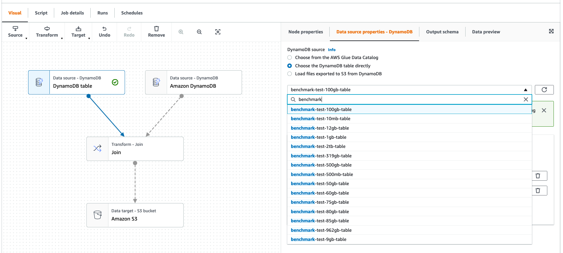
When you want to define your own data integration pipeline, you need to add more AWS Glue jobs and implement job scripts. For this post, let’s assume the use case to add a new AWS Glue job with a new job script to read multiple S3 locations and join them.

Implement and test in your local environment

First, implement and test the AWS Glue job and its job script in your local environment using Visual Studio Code.

Set up your development environment by following the steps in Develop and test AWS Glue version 3.0 and 4.0 jobs locally using a Docker container. The following steps are required in the context of this post:

  1. Start Docker.
  2. Pull the Docker image that has the local development environment using the AWS Glue ETL library:
    $ docker pull public.ecr.aws/glue/aws-glue-libs:glue_libs_4.0.0_image_01

  3. Run the following command to define the AWS named profile name:
    $ PROFILE_NAME="<DEV-PROFILE>"

  4. Run the following command to make it available with the baseline template:
    $ cd aws-glue-cdk-baseline/
    $ WORKSPACE_LOCATION=$(pwd)

  5. Run the Docker container:
    $ docker run -it -v ~/.aws:/home/glue_user/.aws -v $WORKSPACE_LOCATION:/home/glue_user/workspace/ -e AWS_PROFILE=$PROFILE_NAME -e DISABLE_SSL=true 
    --rm -p 4040:4040 -p 18080:18080 
    --name glue_pyspark public.ecr.aws/glue/aws-glue-libs:glue_libs_4.0.0_image_01 pyspark

  6. Start Visual Studio Code.
  7. Choose Remote Explorer in the navigation pane, then choose the arrow icon of the workspace folder in the container public.ecr.aws/glue/aws-glue-libs:glue_libs_4.0.0_image_01.

If the workspace folder is not shown, choose Open folder and select /home/glue_user/workspace.

Then you will see a view similar to the following screenshot.

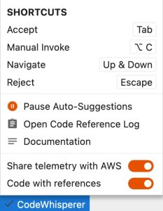
Optionally, you can install AWS Tool Kit for Visual Studio Code, and start Amazon CodeWhisperer to enable code recommendations powered by machine learning model. For example, in aws_glue_cdk_baseline/job_scripts/process_legislators.py, you can put comments like “# Write a DataFrame in Parquet format to S3”, press Enter key, then CodeWhisperer will recommend a code snippet similar to the following:

CodeWhisperer on Visual Studio Code

Now you install the required dependencies described in requirements.txt to the container environment.

  1. Run the following commands in the terminal in Visual Studio Code:
    $ pip install -r requirements.txt
    $ pip install -r requirements-dev.txt

  2. Implement the code.

Now let’s make the required changes for a new AWS Glue job here.

  1. Edit the file aws_glue_cdk_baseline/glue_app_stack.py. Let’s add the following new code block after the existing job definition of ProcessLegislators in order to add the new AWS Glue job JoinLegislators:
            self.new_glue_job = glue.Job(self, "JoinLegislators",
                executable=glue.JobExecutable.python_etl(
                    glue_version=glue.GlueVersion.V4_0,
                    python_version=glue.PythonVersion.THREE,
                    script=glue.Code.from_asset(
                        path.join(path.dirname(__file__), "job_scripts/join_legislators.py")
                    )
                ),
                description="a new example PySpark job",
                default_arguments={
                    "--input_path_orgs": config[stage]['jobs']['JoinLegislators']['inputLocationOrgs'],
                    "--input_path_persons": config[stage]['jobs']['JoinLegislators']['inputLocationPersons'],
                    "--input_path_memberships": config[stage]['jobs']['JoinLegislators']['inputLocationMemberships']
                },
                tags={
                    "environment": self.environment,
                    "artifact_id": self.artifact_id,
                    "stack_id": self.stack_id,
                    "stack_name": self.stack_name
                }
            )

Here, you added three job parameters for different S3 locations using the variable config. It is the dictionary generated from default-config.yaml. In this baseline template, we use this central config file for managing parameters for all the Glue jobs in the structure <stage name>/jobs/<job name>/<parameter name>. In the proceeding steps, you provide those locations through the AWS Glue job parameters.

  1. Create a new job script called aws_glue_cdk_baseline/job_scripts/join_legislators.py:
    aws_glue_cdk_baseline/job_scripts/join_legislators.py:
    
    import sys
    from pyspark.context import SparkContext
    from awsglue.context import GlueContext
    from awsglue.job import Job
    from awsglue.transforms import Join
    from awsglue.utils import getResolvedOptions
    
    
    class JoinLegislators:
        def __init__(self):
            params = []
            if '--JOB_NAME' in sys.argv:
                params.append('JOB_NAME')
                params.append('input_path_orgs')
                params.append('input_path_persons')
                params.append('input_path_memberships')
            args = getResolvedOptions(sys.argv, params)
    
            self.context = GlueContext(SparkContext.getOrCreate())
            self.job = Job(self.context)
    
            if 'JOB_NAME' in args:
                jobname = args['JOB_NAME']
                self.input_path_orgs = args['input_path_orgs']
                self.input_path_persons = args['input_path_persons']
                self.input_path_memberships = args['input_path_memberships']
            else:
                jobname = "test"
                self.input_path_orgs = "s3://awsglue-datasets/examples/us-legislators/all/organizations.json"
                self.input_path_persons = "s3://awsglue-datasets/examples/us-legislators/all/persons.json"
                self.input_path_memberships = "s3://awsglue-datasets/examples/us-legislators/all/memberships.json"
            self.job.init(jobname, args)
        
        def run(self):
            dyf = join_legislators(self.context, self.input_path_orgs, self.input_path_persons, self.input_path_memberships)
            df = dyf.toDF()
            df.printSchema()
            df.show()
            print(df.count())
    
    def read_dynamic_frame_from_json(glue_context, path):
        return glue_context.create_dynamic_frame.from_options(
            connection_type='s3',
            connection_options={
                'paths': [path],
                'recurse': True
            },
            format='json'
        )
    
    def join_legislators(glue_context, path_orgs, path_persons, path_memberships):
        orgs = read_dynamic_frame_from_json(glue_context, path_orgs)
        persons = read_dynamic_frame_from_json(glue_context, path_persons)
        memberships = read_dynamic_frame_from_json(glue_context, path_memberships)
        orgs = orgs.drop_fields(['other_names', 'identifiers']).rename_field('id', 'org_id').rename_field('name', 'org_name')
        dynamicframe_joined = Join.apply(orgs, Join.apply(persons, memberships, 'id', 'person_id'), 'org_id', 'organization_id').drop_fields(['person_id', 'org_id'])
        return dynamicframe_joined
    
    if __name__ == '__main__':
        JoinLegislators().run()

  2. Create a new unit test script for the new AWS Glue job called aws_glue_cdk_baseline/job_scripts/tests/test_join_legislators.py:
    import pytest
    import sys
    import join_legislators
    from pyspark.context import SparkContext
    from awsglue.context import GlueContext
    from awsglue.job import Job
    from awsglue.utils import getResolvedOptions
    
    @pytest.fixture(scope="module", autouse=True)
    def glue_context():
        sys.argv.append('--JOB_NAME')
        sys.argv.append('test_count')
    
        args = getResolvedOptions(sys.argv, ['JOB_NAME'])
        context = GlueContext(SparkContext.getOrCreate())
        job = Job(context)
        job.init(args['JOB_NAME'], args)
    
        yield(context)
    
    def test_counts(glue_context):
        dyf = join_legislators.join_legislators(glue_context, 
            "s3://awsglue-datasets/examples/us-legislators/all/organizations.json",
            "s3://awsglue-datasets/examples/us-legislators/all/persons.json", 
            "s3://awsglue-datasets/examples/us-legislators/all/memberships.json")
        assert dyf.toDF().count() == 10439

  3. In default-config.yaml, add the following under prod and dev:
     JoinLegislators:
          inputLocationOrgs: "s3://awsglue-datasets/examples/us-legislators/all/organizations.json"
          inputLocationPersons: "s3://awsglue-datasets/examples/us-legislators/all/persons.json"
          inputLocationMemberships: "s3://awsglue-datasets/examples/us-legislators/all/memberships.json"

  4. Add the following under "jobs" in the variable config in tests/unit/test_glue_app_stack.py, tests/unit/test_pipeline_stack.py, and tests/snapshot/test_snapshot_glue_app_stack.py (no need to replace S3 locations):
    ,
                "JoinLegislators": {
                    "inputLocationOrgs": "s3://path_to_data_orgs",
                    "inputLocationPersons": "s3://path_to_data_persons",
                    "inputLocationMemberships": "s3://path_to_data_memberships"
                }

  5. Choose Run at the top right to run the individual job scripts.

If the Run button is not shown, install Python into the container through Extensions in the navigation pane.

  1. For local unit testing, run the following command in the terminal in Visual Studio Code:
    $ cd aws_glue_cdk_baseline/job_scripts/
    $ python3 -m pytest

Then you can verify that the newly added unit test passed successfully.

  1. Run pytest to initialize the snapshot test files by running following command:
    $ cd ../../
    $ python3 -m pytest --snapshot-update

Deploy to the development environment

Complete following steps to deploy the AWS Glue app stack to the development environment and run integration tests there:

  1. Set up access to CodeCommit.
  2. Commit and push your changes to the CodeCommit repo:
    $ git add .
    $ git commit -m "Add the second Glue job"
    $ git push

You can see that the pipeline is successfully triggered.

Integration test

There is nothing required for running the integration test for the newly added AWS Glue job. The integration test script integ_test_glue_app_stack.py runs all the jobs including a specific tag, then verifies the state and its duration. If you want to change the condition or the threshold, you can edit assertions at the end of the integ_test_glue_job method.

Deploy to the production environment

Complete the following steps to deploy the AWS Glue app stack to the production environment:

  1. On the CodePipeline console, navigate to GluePipeline.
  2. Choose Review under the DeployProd stage.
  3. Choose Approve.

Wait for the DeployProd stage to complete, then you can verify the AWS Glue app stack resource in the dev account.

Clean up

To clean up your resources, complete following steps:

  1. Run the following command using the pipeline account:
    $ cdk destroy --profile <PIPELINE-PROFILE>

  2. Delete the AWS Glue app stack in the dev account and prod account.

Conclusion

In this post, you learned how to define the development lifecycle for data integration and how software engineers and data engineers can design an end-to-end development lifecycle using AWS Glue, including development, testing, and CI/CD, through a sample AWS CDK template. You can get started building your own end-to-end development lifecycle for your workload using AWS Glue.


About the author

Noritaka Sekiyama is a Principal Big Data Architect on the AWS Glue team. He works based in Tokyo, Japan. He is responsible for building software artifacts to help customers. In his spare time, he enjoys cycling with his road bike.

Build data integration jobs with AI companion on AWS Glue Studio notebook powered by Amazon CodeWhisperer

Post Syndicated from Noritaka Sekiyama original https://aws.amazon.com/blogs/big-data/build-data-integration-jobs-with-ai-companion-on-aws-glue-studio-notebook-powered-by-amazon-codewhisperer/

Data is essential for businesses to make informed decisions, improve operations, and innovate. Integrating data from different sources can be a complex and time-consuming process. AWS offers AWS Glue to help you integrate your data from multiple sources on serverless infrastructure for analysis, machine learning (ML), and application development. AWS Glue provides different authoring experiences for you to build data integration jobs. One of the most common options is the notebook. Data scientists tend to run queries interactively and retrieve results immediately to author data integration jobs. This interactive experience can accelerate building data integration pipelines.

Recently, AWS announced general availability of Amazon CodeWhisperer. Amazon CodeWhisperer is an AI coding companion that uses foundational models under the hood to improve developer productivity. This works by generating code suggestions in real time based on developers’ comments in natural language and prior code in their integrated development environment (IDE). AWS also announced the Amazon CodeWhisperer Jupyter extension to help Jupyter users by generating real-time, single-line, or full-function code suggestions for Python notebooks on Jupyter Lab and Amazon SageMaker Studio.

Today, we are excited to announce that AWS Glue Studio notebooks now support Amazon CodeWhisperer for AWS Glue users to improve your experience and help boost development productivity. Now, in your Glue Studio notebook, you can write a comment in natural language (in English) that outlines a specific task, such as “Create a Spark DataFrame from a json file.”. Based on this information, CodeWhisperer recommends one or more code snippets directly in the notebook that can accomplish the task. You can quickly accept the top suggestion, view more suggestions, or continue writing your own code.

This post demonstrates how the user experience on AWS Glue Studio notebook has been changed with the Amazon CodeWhisperer integration.

Prerequisites

Before going forward with this tutorial, you need to complete the following prerequisites:

  1. Set up AWS Glue Studio.
  2. Configure an AWS Identity and Access Management (IAM) role to interact with Amazon CodeWhisperer. Attach the following policy to your IAM role for the AWS Glue Studio notebook:
    {
        "Version": "2012-10-17",
        "Statement": [
            {
                "Sid": "CodeWhispererPermissions",
                "Effect": "Allow",
                "Action": [
                    "codewhisperer:GenerateRecommendations"
                ],
                "Resource": "*"
            }
        ]
    }

Getting Started

Let’s get started. Create a new AWS Glue Studio notebook job by completing the following steps:

  1. On the AWS Glue console, choose Notebooks under ETL jobs in the navigation pane.
  2. Select Jupyter Notebook and choose Create.
  3. For Job name, enter codewhisperer-demo.
  4. For IAM Role, select your IAM role that you configured as a prerequisite.
  5. Choose Start notebook.

A new notebook is created with sample cells.

At the bottom, there is a menu named CodeWhisperer. By choosing this menu, you can see the shortcuts and several options, including disabling auto-suggestions.

Let’s try your first recommendation by Amazon CodeWhisperer. Note that this post contains examples of recommendations, but you may see different code snippets recommended by Amazon CodeWhisperer.

Add a new cell and enter your comment to describe what you want to achieve. After you press Enter, the recommended code is shown.

If you press Tab, then code is chosen. If you press arrow keys, then you can select other recommendations. You can learn more in User actions.

Now let’s read a JSON file from Amazon Simple Storage Service (Amazon S3). Enter the following code comment into a notebook cell and press Enter:

# Create a Spark DataFrame from a json file

CodeWhisperer will recommend a code snippet similar to the following:

def create_spark_df_from_json(spark, file_path):
    return spark.read.json(file_path)

Now use this method to utilize the suggested code snippet:

df = create_spark_df_from_json(spark, "s3://awsglue-datasets/examples/us-legislators/all/persons.json")
df.show()

The proceeding code returns the following output:

+----------+--------------------+----------+-----------+------+----------+--------------------+--------------------+--------------------+--------------------+--------------------+------------------+--------------------+----------------+
|birth_date|     contact_details|death_date|family_name|gender|given_name|                  id|         identifiers|               image|              images|               links|              name|         other_names|       sort_name|
+----------+--------------------+----------+-----------+------+----------+--------------------+--------------------+--------------------+--------------------+--------------------+------------------+--------------------+----------------+
|1944-10-15|                null|      null|    Collins|  male|   Michael|0005af3a-9471-4d1...|[{C000640, biogui...|https://theunited...|[{https://theunit...|[{Wikipedia (de),...|       Mac Collins|[{bar, Mac Collin...|Collins, Michael|
|1969-01-31|[{fax, 202-226-07...|      null|   Huizenga|  male|      Bill|00aa2dc0-bfb6-441...|[{Bill Huizenga, ...|https://theunited...|[{https://theunit...|[{Wikipedia (de),...|     Bill Huizenga|[{da, Bill Huizen...|  Huizenga, Bill|
|1959-09-28|[{phone, 202-225-...|      null|    Clawson|  male|    Curtis|00aca284-9323-495...|[{C001102, biogui...|https://theunited...|[{https://theunit...|[{Wikipedia (comm...|      Curt Clawson|[{bar, Curt Claws...| Clawson, Curtis|
|1930-08-14|                null|2001-10-26|    Solomon|  male|    Gerald|00b73df5-4180-441...|[{S000675, biogui...|https://theunited...|[{https://theunit...|[{Wikipedia (de),...|    Gerald Solomon|[{null, Gerald B....| Solomon, Gerald|
|1960-05-28|[{fax, 202-225-42...|      null|     Rigell|  male|    Edward|00bee44f-db04-4a7...|[{R000589, biogui...|https://theunited...|[{https://theunit...|[{Wikipedia (de),...|   E. Scott Rigell|[{null, Scott Rig...|  Rigell, Edward|
|1951-05-20|[{twitter, MikeCr...|      null|      Crapo|  male|   Michael|00f8f12d-6e27-4a2...|[{Mike Crapo, bal...|https://theunited...|[{https://theunit...|[{Wikipedia (da),...|        Mike Crapo|[{da, Mike Crapo,...|  Crapo, Michael|
|1926-05-12|                null|      null|      Hutto|  male|      Earl|015d77c8-6edb-4ed...|[{H001018, biogui...|https://theunited...|[{https://theunit...|[{Wikipedia (de),...|        Earl Hutto|[{null, Earl Dewi...|     Hutto, Earl|
|1937-11-07|                null|2015-11-19|      Ertel|  male|     Allen|01679bc3-da21-482...|[{E000208, biogui...|https://theunited...|[{https://theunit...|[{Wikipedia (de),...|       Allen Ertel|[{null, Allen E. ...|    Ertel, Allen|
|1916-09-01|                null|2007-11-24|     Minish|  male|    Joseph|018247d0-2961-423...|[{M000796, biogui...|https://theunited...|[{https://theunit...|[{Wikipedia (de),...|     Joseph Minish|[{bar, Joseph Min...|  Minish, Joseph|
|1957-08-04|[{phone, 202-225-...|      null|    Andrews|  male|    Robert|01b100ac-192e-4b5...|[{A000210, biogui...|https://theunited...|[{https://theunit...|[{Wikipedia (de),...| Robert E. Andrews|[{null, Rob Andre...| Andrews, Robert|
|1957-01-10|[{fax, 202-225-57...|      null|     Walden|  male|      Greg|01bc21bf-8939-487...|[{Greg Walden, ba...|https://theunited...|[{https://theunit...|[{Wikipedia (comm...|       Greg Walden|[{bar, Greg Walde...|    Walden, Greg|
|1919-01-17|                null|1987-11-29|      Kazen|  male|   Abraham|02059c1e-0bdf-481...|[{K000025, biogui...|https://theunited...|[{https://theunit...|[{Wikipedia (de),...|Abraham Kazen, Jr.|[{null, Abraham K...|  Kazen, Abraham|
|1960-01-11|[{fax, 202-225-67...|      null|     Turner|  male|   Michael|020aa7dd-54ef-435...|[{Michael R. Turn...|https://theunited...|[{https://theunit...|[{Wikipedia (comm...| Michael R. Turner|[{null, Mike Turn...| Turner, Michael|
|1942-06-28|                null|      null|      Kolbe|  male|     James|02141651-eca2-4aa...|[{K000306, biogui...|https://theunited...|[{https://theunit...|[{Wikipedia (de),...|         Jim Kolbe|[{ca, Jim Kolbe, ...|    Kolbe, James|
|1941-03-08|[{fax, 202-225-79...|      null|  Lowenthal|  male|      Alan|0231c6ef-6e92-49b...|[{Alan Lowenthal,...|https://theunited...|[{https://theunit...|[{Wikipedia (de),...| Alan S. Lowenthal|[{null, Alan Lowe...| Lowenthal, Alan|
|1952-01-09|[{fax, 202-225-93...|      null|    Capuano|  male|   Michael|0239032f-be5c-4af...|[{Michael Capuano...|https://theunited...|[{https://theunit...|[{Wikipedia (de),...|Michael E. Capuano|[{null, Mike Capu...|Capuano, Michael|
|1951-10-19|[{fax, 202-225-56...|      null|   Schrader|  male|      Kurt|0263f619-eff8-4e1...|[{Kurt Schrader, ...|https://theunited...|[{https://theunit...|[{Wikipedia (de),...|     Kurt Schrader|[{bar, Kurt Schra...|  Schrader, Kurt|
|1947-06-13|[{fax, 202-225-69...|      null|     Nadler|  male|   Jerrold|029e793d-ec40-4a1...|[{N000002, biogui...|https://theunited...|[{https://theunit...|[{Wikipedia (de),...|    Jerrold Nadler|[{ca, Jerrold Nad...| Nadler, Jerrold|
|1970-02-03|[{fax, 202-225-82...|      null|     Graves|  male|       Tom|02b621fc-0523-449...|[{Tom Graves, bal...|https://theunited...|[{https://theunit...|[{Wikipedia (de),...|        Tom Graves|[{bar, Tom Graves...|     Graves, Tom|
|1932-05-09|                null|      null|   McMillan|  male|      John|03018f7c-f866-419...|[{M000566, biogui...|https://theunited...|[{https://theunit...|[{Wikipedia (de),...|     John McMillan|[{null, Alex McMi...|  McMillan, John|
+----------+--------------------+----------+-----------+------+----------+--------------------+--------------------+--------------------+--------------------+--------------------+------------------+--------------------+----------------+
only showing top 20 rows

As you can see from the result, you can quickly utilize the code snippet recommended by Amazon CodeWhisperer.

Examples of code recommendations

In this section, we provide additional examples of code recommendations. Note that these are just our examples, and different code snippets may be suggested by Amazon CodeWhisperer.

Add a column with a calculation

In extract, transform, and load (ETL) use cases, it’s common to add new columns from existing columns. When we need to add columns to our Spark DataFrame, we can articulate with a high level of detail to Amazon CodeWhisperer what type of column we need added and its respective attributes:

# Add age column to a given person DataFrame
# age is calculated from current date and birth_date. When death_date is not null, then use death_date to calculate age

Amazon CodeWhisperer will recommend a code snippet similar to the following:

def add_age_column(df):
    # Use current date to calculate age
    current_date = current_timestamp()
    # Use birth_date column to calculate age
    df = df.withColumn("age", datediff(current_date, df.birth_date) / 365)
    # Use death_date column to calculate age
    df = df.withColumn("age", when(df.death_date.isNull(), df.age).otherwise(datediff(df.death_date, df.birth_date) / 365))
    return df

It can be utilized as follows:

df = add_age_column(df)
df.show()

The preceding code returns the following output:

+----------+--------------------+----------+-----------+------+----------+--------------------+--------------------+--------------------+--------------------+--------------------+------------------+--------------------+----------------+------------------+--------------------+
|birth_date|     contact_details|death_date|family_name|gender|given_name|                  id|         identifiers|               image|              images|               links|              name|         other_names|       sort_name|               age|        current_date|
+----------+--------------------+----------+-----------+------+----------+--------------------+--------------------+--------------------+--------------------+--------------------+------------------+--------------------+----------------+------------------+--------------------+
|1944-10-15|                null|      null|    Collins|  male|   Michael|0005af3a-9471-4d1...|[{C000640, biogui...|https://theunited...|[{https://theunit...|[{Wikipedia (de),...|       Mac Collins|[{bar, Mac Collin...|Collins, Michael| 78.71506849315068|2023-06-14 06:12:...|
|1969-01-31|[{fax, 202-226-07...|      null|   Huizenga|  male|      Bill|00aa2dc0-bfb6-441...|[{Bill Huizenga, ...|https://theunited...|[{https://theunit...|[{Wikipedia (de),...|     Bill Huizenga|[{da, Bill Huizen...|  Huizenga, Bill|  54.4027397260274|2023-06-14 06:12:...|
|1959-09-28|[{phone, 202-225-...|      null|    Clawson|  male|    Curtis|00aca284-9323-495...|[{C001102, biogui...|https://theunited...|[{https://theunit...|[{Wikipedia (comm...|      Curt Clawson|[{bar, Curt Claws...| Clawson, Curtis| 63.75342465753425|2023-06-14 06:12:...|
|1930-08-14|                null|2001-10-26|    Solomon|  male|    Gerald|00b73df5-4180-441...|[{S000675, biogui...|https://theunited...|[{https://theunit...|[{Wikipedia (de),...|    Gerald Solomon|[{null, Gerald B....| Solomon, Gerald| 71.24931506849315|2023-06-14 06:12:...|
|1960-05-28|[{fax, 202-225-42...|      null|     Rigell|  male|    Edward|00bee44f-db04-4a7...|[{R000589, biogui...|https://theunited...|[{https://theunit...|[{Wikipedia (de),...|   E. Scott Rigell|[{null, Scott Rig...|  Rigell, Edward|63.087671232876716|2023-06-14 06:12:...|
|1951-05-20|[{twitter, MikeCr...|      null|      Crapo|  male|   Michael|00f8f12d-6e27-4a2...|[{Mike Crapo, bal...|https://theunited...|[{https://theunit...|[{Wikipedia (da),...|        Mike Crapo|[{da, Mike Crapo,...|  Crapo, Michael| 72.11780821917809|2023-06-14 06:12:...|
|1926-05-12|                null|      null|      Hutto|  male|      Earl|015d77c8-6edb-4ed...|[{H001018, biogui...|https://theunited...|[{https://theunit...|[{Wikipedia (de),...|        Earl Hutto|[{null, Earl Dewi...|     Hutto, Earl| 97.15616438356165|2023-06-14 06:12:...|
|1937-11-07|                null|2015-11-19|      Ertel|  male|     Allen|01679bc3-da21-482...|[{E000208, biogui...|https://theunited...|[{https://theunit...|[{Wikipedia (de),...|       Allen Ertel|[{null, Allen E. ...|    Ertel, Allen| 78.08493150684932|2023-06-14 06:12:...|
|1916-09-01|                null|2007-11-24|     Minish|  male|    Joseph|018247d0-2961-423...|[{M000796, biogui...|https://theunited...|[{https://theunit...|[{Wikipedia (de),...|     Joseph Minish|[{bar, Joseph Min...|  Minish, Joseph|  91.2904109589041|2023-06-14 06:12:...|
|1957-08-04|[{phone, 202-225-...|      null|    Andrews|  male|    Robert|01b100ac-192e-4b5...|[{A000210, biogui...|https://theunited...|[{https://theunit...|[{Wikipedia (de),...| Robert E. Andrews|[{null, Rob Andre...| Andrews, Robert|  65.9041095890411|2023-06-14 06:12:...|
|1957-01-10|[{fax, 202-225-57...|      null|     Walden|  male|      Greg|01bc21bf-8939-487...|[{Greg Walden, ba...|https://theunited...|[{https://theunit...|[{Wikipedia (comm...|       Greg Walden|[{bar, Greg Walde...|    Walden, Greg| 66.46849315068494|2023-06-14 06:12:...|
|1919-01-17|                null|1987-11-29|      Kazen|  male|   Abraham|02059c1e-0bdf-481...|[{K000025, biogui...|https://theunited...|[{https://theunit...|[{Wikipedia (de),...|Abraham Kazen, Jr.|[{null, Abraham K...|  Kazen, Abraham| 68.91232876712328|2023-06-14 06:12:...|
|1960-01-11|[{fax, 202-225-67...|      null|     Turner|  male|   Michael|020aa7dd-54ef-435...|[{Michael R. Turn...|https://theunited...|[{https://theunit...|[{Wikipedia (comm...| Michael R. Turner|[{null, Mike Turn...| Turner, Michael|63.465753424657535|2023-06-14 06:12:...|
|1942-06-28|                null|      null|      Kolbe|  male|     James|02141651-eca2-4aa...|[{K000306, biogui...|https://theunited...|[{https://theunit...|[{Wikipedia (de),...|         Jim Kolbe|[{ca, Jim Kolbe, ...|    Kolbe, James| 81.01643835616439|2023-06-14 06:12:...|
|1941-03-08|[{fax, 202-225-79...|      null|  Lowenthal|  male|      Alan|0231c6ef-6e92-49b...|[{Alan Lowenthal,...|https://theunited...|[{https://theunit...|[{Wikipedia (de),...| Alan S. Lowenthal|[{null, Alan Lowe...| Lowenthal, Alan| 82.32328767123288|2023-06-14 06:12:...|
|1952-01-09|[{fax, 202-225-93...|      null|    Capuano|  male|   Michael|0239032f-be5c-4af...|[{Michael Capuano...|https://theunited...|[{https://theunit...|[{Wikipedia (de),...|Michael E. Capuano|[{null, Mike Capu...|Capuano, Michael| 71.47671232876712|2023-06-14 06:12:...|
|1951-10-19|[{fax, 202-225-56...|      null|   Schrader|  male|      Kurt|0263f619-eff8-4e1...|[{Kurt Schrader, ...|https://theunited...|[{https://theunit...|[{Wikipedia (de),...|     Kurt Schrader|[{bar, Kurt Schra...|  Schrader, Kurt|  71.7013698630137|2023-06-14 06:12:...|
|1947-06-13|[{fax, 202-225-69...|      null|     Nadler|  male|   Jerrold|029e793d-ec40-4a1...|[{N000002, biogui...|https://theunited...|[{https://theunit...|[{Wikipedia (de),...|    Jerrold Nadler|[{ca, Jerrold Nad...| Nadler, Jerrold| 76.05479452054794|2023-06-14 06:12:...|
|1970-02-03|[{fax, 202-225-82...|      null|     Graves|  male|       Tom|02b621fc-0523-449...|[{Tom Graves, bal...|https://theunited...|[{https://theunit...|[{Wikipedia (de),...|        Tom Graves|[{bar, Tom Graves...|     Graves, Tom|53.394520547945206|2023-06-14 06:12:...|
|1932-05-09|                null|      null|   McMillan|  male|      John|03018f7c-f866-419...|[{M000566, biogui...|https://theunited...|[{https://theunit...|[{Wikipedia (de),...|     John McMillan|[{null, Alex McMi...|  McMillan, John| 91.15890410958905|2023-06-14 06:12:...|
+----------+--------------------+----------+-----------+------+----------+--------------------+--------------------+--------------------+--------------------+--------------------+------------------+--------------------+----------------+------------------+--------------------+
only showing top 20 rows

Sort and extract records

You can use Amazon CodeWhisperer for sorting data and extracting records within a Spark DataFrame as well:

# Show top 5 oldest persons from DataFrame
# Use age column

Amazon CodeWhisperer will recommend a code snippet similar to the following:

def get_oldest_person(df):
    return df.orderBy(desc("age")).limit(5)

It can be utilized as follows:

get_oldest_person(df).show()

The preceding code returns the following output:

+----------+---------------+----------+-----------+------+----------+--------------------+--------------------+--------------------+--------------------+--------------------+---------------+--------------------+---------------+------------------+--------------------+
|birth_date|contact_details|death_date|family_name|gender|given_name|                  id|         identifiers|               image|              images|               links|           name|         other_names|      sort_name|               age|        current_date|
+----------+---------------+----------+-----------+------+----------+--------------------+--------------------+--------------------+--------------------+--------------------+---------------+--------------------+---------------+------------------+--------------------+
|1919-08-22|           null|      null|       Winn|  male|    Edward|942d20ed-d838-436...|[{W000636, biogui...|https://theunited...|[{https://theunit...|[{Wikipedia (de),...|Larry Winn, Jr.|[{null, Larry Win...|   Winn, Edward|103.88219178082191|2023-06-14 06:13:...|
|1920-03-23|           null|      null|      Smith|  male|      Neal|84a9cbe4-651b-46d...|[{S000596, biogui...|https://theunited...|[{https://theunit...|[{Wikipedia (de),...|     Neal Smith|[{null, Neal Edwa...|    Smith, Neal| 103.2958904109589|2023-06-14 06:13:...|
|1920-09-17|           null|      null|       Holt|female|  Marjorie|8bfb671a-3147-4bc...|[{H000747, biogui...|https://theunited...|[{https://theunit...|[{Wikipedia (de),...|  Marjorie Holt|[{bar, Marjorie H...| Holt, Marjorie| 102.8082191780822|2023-06-14 06:13:...|
|1921-03-05|           null|      null|     Bedell|  male|   Berkley|896f0ce3-afe4-4ea...|[{B000298, biogui...|https://theunited...|[{https://theunit...|[{Wikipedia (de),...| Berkley Bedell|[{ca, Berkley Bed...|Bedell, Berkley|102.34520547945205|2023-06-14 06:13:...|
|1921-06-23|           null|      null|    Findley|  male|      Paul|2811f793-1108-4fb...|[{F000123, biogui...|https://theunited...|[{https://theunit...|[{Wikipedia (azb)...|   Paul Findley|[{azb, پاول فایند...|  Findley, Paul|102.04383561643836|2023-06-14 06:13:...|
+----------+---------------+----------+-----------+------+----------+--------------------+--------------------+--------------------+--------------------+--------------------+---------------+--------------------+---------------+------------------+--------------------+

Generate sample datasets in a Spark DataFrame

Amazon CodeWhisperer is powerful enough to generate sample Spark DataFrames as well, which can be done like so:

# Generate sample Spark DataFrame of country name and country code
# First column name is country_name, and second column name is country_code

Amazon CodeWhisperer will recommend a code snippet similar to the following:

def get_country_code_df(spark):
    return spark.createDataFrame(
        [("United States", "US"), ("United Kingdom", "UK"), ("Canada", "CA")],
        ["country_name", "country_code"]
    )

It can be utilized as follows:

df = get_country_code_df(spark)
df.show()

The preceding code returns the following output:

+--------------+------------+
|  country_name|country_code|
+--------------+------------+
| United States|          US|
|United Kingdom|          UK|
|        Canada|          CA|
+--------------+------------+

Generate transformations in SQL

We can also use Amazon CodeWhisperer to create a code snippet for transformation in SQL and create a new table from the SQL query results (CTAS) like so:

# Generate CTAS query by selecting all the records in a table with grouping by a given column

Amazon CodeWhisperer will recommend a code snippet similar to following:

def generate_ctas_query_with_group_by(table_name, group_by_col):
    ctas_query = "CREATE TABLE " + table_name + " AS SELECT * FROM " + table_name + " GROUP BY " + group_by_col
    return ctas_query

Conclusion

In this post, we demonstrated how AWS Glue Studio notebook integration with Amazon CodeWhisperer helps you build data integration jobs faster. This integration is available today in US East (N. Virginia). You can start using the AWS Glue Studio notebook with Amazon CodeWhisperer to accelerate building your data integration jobs. To get started with AWS Glue, visit AWS Glue.

Learn more

To learn more about using AWS Glue notebooks and Amazon CodeWhisperer, check out the following video.


About the authors

Noritaka Sekiyama is a Principal Big Data Architect on the AWS Glue team. He works based in Tokyo, Japan. He is responsible for building software artifacts to help customers. In his spare time, he enjoys cycling with his road bike.

Gal blog picGal Heyne is a Product Manager for AWS Glue with a strong focus on AI/ML, data engineering, and BI, and is based in California. She is passionate about developing a deep understanding of customers’ business needs and collaborating with engineers to design easy-to-use data products. In her spare time, she enjoys playing card games.

Scale your AWS Glue for Apache Spark jobs with new larger worker types G.4X and G.8X

Post Syndicated from Noritaka Sekiyama original https://aws.amazon.com/blogs/big-data/scale-your-aws-glue-for-apache-spark-jobs-with-new-larger-worker-types-g-4x-and-g-8x/

Hundreds of thousands of customers use AWS Glue, a serverless data integration service, to discover, prepare, and combine data for analytics, machine learning (ML), and application development. AWS Glue for Apache Spark jobs work with your code and configuration of the number of data processing units (DPU). Each DPU provides 4 vCPU, 16 GB memory, and 64 GB disk. AWS Glue manages running Spark and adjusts workers to achieve the best price performance. For workloads such as data transforms, joins, and queries, you can use G.1X (1 DPU) and G.2X (2 DPU) workers, which offer a scalable and cost-effective way to run most jobs. With exponentially growing data sources and data lakes, customers want to run more data integration workloads, including their most demanding transforms, aggregations, joins, and queries. These workloads require higher compute, memory, and storage per worker.

Today we are pleased to announce the general availability of AWS Glue G.4X (4 DPU) and G.8X (8 DPU) workers, the next series of AWS Glue workers for the most demanding data integration workloads. G.4X and G.8X workers offer increased compute, memory, and storage, making it possible for you to vertically scale and run intensive data integration jobs, such as memory-intensive data transforms, skewed aggregations, and entity detection checks involving petabytes of data. Larger worker types not only benefit the Spark executors, but also in cases where the Spark driver needs larger capacity—for instance, because the job query plan is quite large.

This post demonstrates how AWS Glue G.4X and G.8X workers help you scale your AWS Glue for Apache Spark jobs.

G.4X and G.8X workers

AWS Glue G.4X and G.8X workers give you more compute, memory, and storage to run your most demanding jobs. G.4X workers provide 4 DPU, with 16 vCPU, 64 GB memory, and 256 GB of disk per node. G.8X workers provide 8 DPU, with 32 vCPU, 128 GB memory, and 512 GB of disk per node. You can enable G.4X and G.8X workers with a single parameter change in the API, AWS Command Line Interface (AWS CLI), or visually in AWS Glue Studio. Regardless of the worker used, all AWS Glue jobs have the same capabilities, including auto scaling and interactive job authoring via notebooks. G.4X and G.8X workers are available with AWS Glue 3.0 and 4.0.

The following table shows compute, memory, disk, and Spark configurations per worker type in AWS Glue 3.0 or later.

AWS Glue Worker Type DPU per Node vCPU Memory (GB) Disk (GB) Number of Spark Executors per Node Number of Cores per Spark Executor
G.1X 1 4 16 64 1 4
G.2X 2 8 32 128 1 8
G.4X (new) 4 16 64 256 1 16
G.8X (new) 8 32 128 512 1 32

To use G.4X and G.8X workers on an AWS Glue job, change the setting of the worker type parameter to G.4X or G.8X. In AWS Glue Studio, you can choose G 4X or G 8X under Worker type.

In the AWS API or AWS SDK, you can specify G.4X or G.8X in the WorkerType parameter. In the AWS CLI, you can use the --worker-type parameter in a create-job command.

To use G.4X and G.8X on an AWS Glue Studio notebook or interactive sessions, set G.4X or G.8X in the %worker_type magic:

Performance characteristics using the TPC-DS benchmark

In this section, we use the TPC-DS benchmark to showcase performance characteristics of the new G.4X and G.8X worker types. We used AWS Glue version 4.0 jobs.

G.2X, G.4X, and G.8X results with the same number of workers

Compared to the G.2X worker type, the G.4X worker has 2 times the DPUs and the G.8X worker has 4 times the DPUs. We ran over 100 TPC-DS queries against the 3 TB TPC-DS dataset with the same number of workers but on different worker types. The following table shows the results of the benchmark.

Worker Type Number of Workers Number of DPUs Duration (minutes) Cost at $0.44/DPU-hour ($)
G.2X 30 60 537.4 $236.46
G.4X 30 120 264.6 $232.85
G.8X 30 240 122.6 $215.78

When running jobs on the same number of workers, the new G.4X and G.8x workers achieved roughly linear vertical scalability.

G.2X, G.4X, and G.8X results with the same number of DPUs

We ran over 100 TPC-DS queries against the 10 TB TPC-DS dataset with the same number of DPUs but on different worker types. The following table shows the results of the experiments.

Worker Type Number of Workers Number of DPUs Duration (minutes) Cost at $0.44/DPU-hour ($)
G.2X 40 80 1323 $776.16
G.4X 20 80 1191 $698.72
G.8X 10 80 1190 $698.13

When running jobs on the same number of total DPUs, the job performance stayed mostly the same with new worker types.

Example: Memory-intensive transformations

Data transformations are an essential step to preprocess and structure your data into an optimal form. Bigger memory footprints are consumed in some transformations such as aggregation, join, your own custom logic using user-defined functions (UDFs), and so on. The new G.4X and G.8X workers enable you to run larger memory-intensive transformations at scale.

The following example reads large JSON files compressed in GZIP from an input Amazon Simple Storage Service (Amazon S3) location, performs groupBy, calculates groups based on K-means clustering using a Pandas UDF, then shows the results. Note that this UDF-based K-means is used just for illustration purposes; it’s recommended to use native K-means clustering for production purposes.

With G.2X workers

When an AWS Glue job runs on 12 G.2X workers (24 DPU), it failed due to a No space left on device error. On the Spark UI, the Stages tab for the failed stage shows that there were multiple failed tasks in the AWS Glue job due to the error.

The Executor tab shows failed tasks per executor.

Generally, G.2X workers can process memory-intensive workload well. This time, we used a special Pandas UDF that consumes a significant amount of memory, and it caused a failure due to a large amount of shuffle writes.

With G.8X workers

When an AWS Glue job runs on 3 G.8X workers (24 DPU), it succeeded without any failures, as shown on the Spark UI’s Jobs tab.

The Executors tab also explains that there were no failed tasks.

From this result, we observed that G.8X workers processed the same workload without failures.

Conclusion

In this post, we demonstrated how AWS Glue G.4X and G.8X workers can help you vertically scale your AWS Glue for Apache Spark jobs. G.4X and G.8X workers are available today in US East (Ohio), US East (N. Virginia), US West (Oregon), Asia Pacific (Singapore), Asia Pacific (Sydney), Asia Pacific (Tokyo), Canada (Central), Europe (Frankfurt), Europe (Ireland), and Europe (Stockholm). You can start using the new G.4X and G.8X worker types to scale your workload from today. To get started with AWS Glue, visit AWS Glue.


About the authors

Noritaka Sekiyama is a Principal Big Data Architect on the AWS Glue team. He works based in Tokyo, Japan. He is responsible for building software artifacts to help customers. In his spare time, he enjoys cycling with his road bike.

Tomohiro Tanaka is a Senior Cloud Support Engineer on the AWS Support team. He’s passionate about helping customers build data lakes using ETL workloads. In his free time, he enjoys coffee breaks with his colleagues and making coffee at home.

Chuhan LiuChuhan Liu is a Software Development Engineer on the AWS Glue team. He is passionate about building scalable distributed systems for big data processing, analytics, and management. In his spare time, he enjoys playing tennis.

Matt Su is a Senior Product Manager on the AWS Glue team. He enjoys helping customers uncover insights and make better decisions using their data with AWS Analytic services. In his spare time, he enjoys skiing and gardening.

Introducing native support for Apache Hudi, Delta Lake, and Apache Iceberg on AWS Glue for Apache Spark, Part 2: AWS Glue Studio Visual Editor

Post Syndicated from Noritaka Sekiyama original https://aws.amazon.com/blogs/big-data/part-2-glue-studio-visual-editor-introducing-native-support-for-apache-hudi-delta-lake-and-apache-iceberg-on-aws-glue-for-apache-spark/

In the first post of this series, we described how AWS Glue for Apache Spark works with Apache Hudi, Linux Foundation Delta Lake, and Apache Iceberg datasets tables using the native support of those data lake formats. This native support simplifies reading and writing your data for these data lake frameworks so you can more easily build and maintain your data lakes in a transactionally consistent manner. This feature removes the need to install a separate connector and reduces the configuration steps required to use these frameworks in AWS Glue for Apache Spark jobs.

These data lake frameworks help you store data more efficiently and enable applications to access your data faster. Unlike simpler data file formats such as Apache Parquet, CSV, and JSON, which can store big data, data lake frameworks organize distributed big data files into tabular structures that enable basic constructs of databases on data lakes.

Expanding on the functionality we announced at AWS re:Invent 2022, AWS Glue now natively supports Hudi, Delta Lake and Iceberg through the AWS Glue Studio visual editor. If you prefer authoring AWS Glue for Apache Spark jobs using a visual tool, you can now choose any of these three data lake frameworks as a source or target through a graphical user interface (GUI) without any custom code.

Even without prior experience using Hudi, Delta Lake or Iceberg, you can easily achieve typical use cases. In this post, we demonstrate how to ingest data stored in Hudi using the AWS Glue Studio visual editor.

Example scenario

To demonstrate the visual editor experience, this post introduces the Global Historical Climatology Network Daily (GHCN-D) dataset. The data is publicly accessible through an Amazon Simple Storage Service (Amazon S3) bucket. For more information, see the Registry of Open Data on AWS. You can also learn more in Visualize over 200 years of global climate data using Amazon Athena and Amazon QuickSight.

The Amazon S3 location s3://noaa-ghcn-pds/csv/by_year/ has all the observations from 1763 to the present organized in CSV files, one file for each year. The following block shows an example of what the records look like:

ID,DATE,ELEMENT,DATA_VALUE,M_FLAG,Q_FLAG,S_FLAG,OBS_TIME
AE000041196,20220101,TAVG,204,H,,S,
AEM00041194,20220101,TAVG,211,H,,S,
AEM00041217,20220101,TAVG,209,H,,S,
AEM00041218,20220101,TAVG,207,H,,S,
AE000041196,20220102,TAVG,226,H,,S,
...
AE000041196,20221231,TMAX,243,,,S,
AE000041196,20221231,PRCP,0,D,,S,
AE000041196,20221231,TAVG,202,H,,S,

The records have fields including ID, DATE, ELEMENT, and more. Each combination of ID, DATE, and ELEMENT represents a unique record in this dataset. For example, the record with ID as AE000041196, ELEMENT as TAVG, and DATE as 20220101 is unique.

In this tutorial, we assume that the files are updated with new records every day, and want to store only the latest record per the primary key (ID and ELEMENT) to make the latest snapshot data queryable. One typical approach is to do an INSERT for all the historical data, and calculate the latest records in queries; however, this can introduce additional overhead in all the queries. When you want to analyze only the latest records, it’s better to do an UPSERT (update and insert) based on the primary key and DATE field rather than just an INSERT in order to avoid duplicates and maintain a single updated row of data.

Prerequisites

To continue this tutorial, you need to create the following AWS resources in advance:

Process a Hudi dataset on the AWS Glue Studio visual editor

Let’s author an AWS Glue job to read daily records in 2022, and write the latest snapshot into the Hudi table on your S3 bucket using UPSERT. Complete following steps:

  1. Open AWS Glue Studio.
  2. Choose Jobs.
  3. Choose Visual with a source and target.
  4. For Source and Target, choose Amazon S3, then choose Create.

A new visual job configuration appears. The next step is to configure the data source to read an example dataset:

  1. Under Visual, choose Data source – S3 bucket.
  2. Under Node properties, for S3 source type, select S3 location.
  3. For S3 URL, enter s3://noaa-ghcn-pds/csv/by_year/2022.csv.

The data source is configured.

data-source

The next step is to configure the data target to ingest data in Apache Hudi on your S3 bucket:

  1. Choose Data target – S3 bucket.
  2. Under Data target properties- S3, for Format, choose Apache Hudi.
  3. For Hudi Table Name, enter ghcn.
  4. For Hudi Storage Type, choose Copy on write.
  5. For Hudi Write Operation, choose Upsert.
  6. For Hudi Record Key Fields, choose ID.
  7. For Hudi Precombine Key Field, choose DATE.
  8. For Compression Type, choose GZIP.
  9. For S3 Target location, enter s3://<Your S3 bucket name>/<Your S3 bucket prefix>/hudi_native/ghcn/. (Provide your S3 bucket name and prefix.)

To make it easy to discover the sample data, and also make it queryable from Athena, configure the job to create a table definition on the AWS Glue Data Catalog:

  1. For Data Catalog update options, select Create a table in the Data Catalog and on subsequent runs, update the schema and add new partitions.
  2. For Database, choose hudi_native.
  3. For Table name, enter ghcn.
  4. For Partition keys – optional, choose ELEMENT.

Now your data integration job is authored in the visual editor completely. Let’s add one remaining setting about the IAM role, then run the job:

  1. Under Job details, for IAM Role, choose your IAM role.
  2. Choose Save, then choose Run.

data-target

  1. Navigate to the Runs tab to track the job progress and wait for it to complete.

job-run

Query the table with Athena

Now that the job has successfully created the Hudi table, you can query the table through different engines, including Amazon Athena, Amazon EMR, and Amazon Redshift Spectrum, in addition to AWS Glue for Apache Spark.

To query through Athena, complete the following steps:

  1. On the Athena console, open the query editor.
  2. In the query editor, enter the following SQL and choose Run:
SELECT * FROM "hudi_native"."ghcn" limit 10;

The following screenshot shows the query result.
athena-query1

Let’s dive deep into the table to understand how the data is ingested and focus on the records with ID=’AE000041196′.

  1. Run the following query to focus on the very specific example records with ID='AE000041196':
SELECT * FROM "hudi_native"."ghcn" WHERE ID='AE000041196';

The following screenshot shows the query result.
athena-query2

The original source file 2022.csv has historical records for record ID='USW00012894' from 20220101 to 20221231, however the query result shows only four records, one record per ELEMENT at the latest snapshot of the day 20221230 or 20221231. Because we used the UPSERT write option when writing data, we configured the ID field as a Hudi record key field, the DATE field as a Hudi precombine field, and the ELEMENT field as partition key field. When two records have the same key value, Hudi picks the one with the largest value for the precombine field. When the job ingested data, it compared all the values in the DATE field for each pair of ID and ELEMENT, and then picked the record with the largest value in the DATE field.

According to the preceding result, we were able to ingest the latest snapshot from all the 2022 data. Now let’s do an UPSERT of the new 2023 data to overwrite the records on the target Hudi table.

  1. Go back to AWS Glue Studio console, modify the source S3 location to s3://noaa-ghcn-pds/csv/by_year/2023.csv, then save and run the job.

upsert-data-source

  1. Run the same Athena query from the Athena console.

athena-query3
Now you see that the four records have been updated with the new records in 2023.

If you have further future records, this approach works well to upsert new records based on the Hudi record key and Hudi precombine key.

Clean up

Now to the final step, cleaning up the resources:

  1. Delete the AWS Glue database hudi_native.
  2. Delete the AWS Glue table ghcn.
  3. Delete the S3 objects under s3://<Your S3 bucket name>/<Your S3 bucket prefix>/hudi_native/ghcn2022/.

Conclusion

This post demonstrated how to process Hudi datasets using the AWS Glue Studio visual editor. The AWS Glue Studio visual editor enables you to author jobs while taking advantage of data lake formats and without needing expertise in them. If you have comments or feedback, please feel free to leave them in the comments.


About the authors

Noritaka Sekiyama is a Principal Big Data Architect on the AWS Glue team. He is responsible for building software artifacts to help customers. In his spare time, he enjoys cycling with his new road bike.

Scott Long is a Front End Engineer on the AWS Glue team. He is responsible for implementing new features in AWS Glue Studio. In his spare time, he enjoys socializing with friends and participating in various outdoor activities.

Sean Ma is a Principal Product Manager on the AWS Glue team. He has an 18+ year track record of innovating and delivering enterprise products that unlock the power of data for users. Outside of work, Sean enjoys scuba diving and college football.

Introducing native Delta Lake table support with AWS Glue crawlers

Post Syndicated from Noritaka Sekiyama original https://aws.amazon.com/blogs/big-data/introducing-native-delta-lake-table-support-with-aws-glue-crawlers/

Delta Lake is an open-source project that helps implement modern data lake architectures commonly built on Amazon S3 or other cloud storages. With Delta Lake, you can achieve ACID transactions, time travel queries, CDC, and other common use cases on the cloud. Delta Lake is available with multiple AWS services, such as AWS Glue Spark jobs, Amazon EMR, Amazon Athena, and Amazon Redshift Spectrum.

AWS Glue includes Delta crawler, a capability that makes discovering datasets simpler by scanning Delta Lake transaction logs in Amazon Simple Storage Service (Amazon S3), extracting their schema, creating manifest files in Amazon S3, and automatically populating the AWS Glue Data Catalog, which keeps the metadata current.  The newly created AWS Glue Data Catalog table has format SymlinkTextInputFormat. Delta crawler creates a manifest file, which is a text file containing the list of data files that query engines such as Presto, Trino, or Athena can use to query the table rather than finding the files with the directory listing. A previous blog post demonstrated how it works. Manifest files needed to be regenerated on a periodic basis to include newer transactions in the original Delta Lake tables which resulted in expensive I/O operations, longer processing times, and increased storage footprint.

With today’s launch, Glue crawler is adding support for creating AWS Glue Data Catalog tables for native Delta Lake tables and does not require generating manifest files. This improves customer experience because now you don’t have to regenerate manifest files whenever a new partition becomes available or a table’s metadata changes. With the native Delta Lake tables and automatic schema evolution with no additional manual intervention, this reduces the time to insight by making newly ingested data quickly available for analysis with your preferred analytics and machine learning (ML) tools.

Amazon Athena SQL engine version 3 started supporting Delta Lake native connector. AWS Glue for Apache Spark also started supporting Delta Lake native connector in Glue version 3.0 and later. Amazon EMR started supporting Delta Lake in EMR release version 6.9.0 and later. It means that you can query the Delta transaction log directly in Amazon Athena, AWS Glue for Apache Spark, and Amazon EMR. It makes the experience of working with native Delta Lake tables seamless across the platforms.

This post demonstrates how AWS Glue crawlers work with native Delta Lake tables and describes typical use cases to query native Delta Lake tables.

How AWS Glue crawler works with native Delta Lake tables

Now AWS Glue crawler has two different options:

  • Native table: Create a native Delta Lake table definition on AWS Glue Data Catalog.
  • Symlink table: Create a symlink-based manifest table definition on AWS Glue Data Catalog from a Delta Lake table, and generate its symlink files on Amazon S3.

Native table

Native Delta Lake tables are accessible from Amazon Athena (engine version 3), AWS Glue for Apache Spark (Glue version 3.0 and later), Amazon EMR (release version 6.9.0 and later), and other platforms that support Delta Lake tables. With the native Delta Lake tables, you have the capabilities such as ACID transactions, all while needing to maintain just a single source of truth.

Symlink table

Symlink tables are a consistent snapshot of a native Delta Lake table, represented using the SymlinkTextInputFormat using parquet files. The symlink tables are accessible from Amazon Athena and Amazon Redshift Spectrum.

Since the symlink tables are a snapshot of the original native Delta Lake tables, you need to maintain both the original native Delta Lake tables and the symlink tables. When the data or schema in an original Delta Lake table is updated, the symlink tables in the AWS Glue Data Catalog may become out of sync. It means that you can still query the symlink table and get a consistent result, but the result of the table is at the previous point in time.

Crawl native Delta Lake tables using AWS Glue crawler

In this section, let’s go through how to crawl native Delta Lake tables using AWS Glue crawler.

Prerequisite

Here’s the prerequisite for this tutorial:

  1. Install and configure AWS Command Line Interface (AWS CLI).
  2. Create your S3 bucket if you do not have it.
  3. Create your IAM role for AWS Glue crawler if you do not have it.
  4. Run the following command to copy the sample Delta Lake table into your S3 bucket. (Replace your_s3_bucket with your S3 bucket name.)
$ aws s3 sync s3://aws-bigdata-blog/artifacts/delta-lake-crawler/sample_delta_table/ s3://your_s3_bucket/data/sample_delta_table

Create a Delta Lake crawler

A Delta Lake crawler can be created through the AWS Glue console, AWS Glue SDK, or AWS CLI. Specify a DeltaTarget with the following configurations:

  • DeltaTables – A list of S3 DeltaPaths where the Delta Lake tables are located. (Note that each path must be the parent of a _delta_log folder. If the Delta transaction log is located at s3://bucket/sample_delta_table/_delta_log, then the path s3://bucket/sample_delta_table/ should be provided.
  • WriteManifest – A Boolean value indicating whether or not the crawler should write the manifest files for each DeltaPath. This parameter is only applicable for Delta Lake tables created via manifest files
  • CreateNativeDeltaTable – A Boolean value indicating whether the crawler should create a native Delta Lake table. If set to False, the crawler would create a symlink table instead. Note that both WriteManifest and CreateNativeDeltaTable options can’t be set to True.
  • ConnectionName – An optional connection name stored in the Data Catalog that the crawler should use to access Delta Lake tables backed by a VPC.

In this instruction, create the crawler through the console. Complete the following steps to create a Delta Lake crawler:

  1. Open the AWS Glue console.
  2. Choose Crawlers.
  3. Choose Create crawler.
  4. For Name, enter delta-lake-native-crawler, and choose Next.
  5. Under Data sources, choose Add a data source.
  6. For Data source, select Delta Lake.
  7. For Include delta lake table path(s), enter s3://your_s3_bucket/data/sample_delta_table/.
  8. For Create tables for querying, choose Create Native tables,
  9. Choose Add a Delta Lake data source.
  10. Choose Next.
  11. For Existing IAM role, choose your IAM role, then choose Next.
  12. For Target database, choose Add database, then Add database dialog appears. For Database name, enter delta_lake_native, then choose Create. Choose Next.
  13. Choose Create crawler.
  14. The Delta Lake crawler can be triggered to run through the console or through the SDK or AWS CLI using the StartCrawl API. It could also be scheduled through the console to trigger the crawlers at specific times. In this instruction, run the crawler through the console.
  15. Select delta-lake-native-crawler, and choose Run.
  16. Wait for the crawler to complete.

After the crawler has run, you can see the Delta Lake table definition in the AWS Glue console:

You can also verify an AWS Glue table definition through the following AWS CLI command:

$ aws glue get-table --database delta_lake_native --name sample_delta_table
{
    "Table": {
        "Name": "sample_delta_table",
        "DatabaseName": "delta_lake_native",
        "Owner": "owner",
        "CreateTime": "2022-11-08T12:11:20+09:00",
        "UpdateTime": "2022-11-08T13:19:06+09:00",
        "LastAccessTime": "2022-11-08T13:19:06+09:00",
        "Retention": 0,
        "StorageDescriptor": {
            "Columns": [
                {
                    "Name": "product_id",
                    "Type": "string"
                },
                {
                    "Name": "product_name",
                    "Type": "string"
                },
                {
                    "Name": "price",
                    "Type": "bigint"
                },
                {
                    "Name": "currency",
                    "Type": "string"
                },
                {
                    "Name": "category",
                    "Type": "string"
                },
                {
                    "Name": "updated_at",
                    "Type": "double"
                }
            ],
            "Location": "s3://your_s3_bucket/data/sample_delta_table/",
            "AdditionalLocations": [],
            "InputFormat": "org.apache.hadoop.mapred.SequenceFileInputFormat",
            "OutputFormat": "org.apache.hadoop.hive.ql.io.HiveSequenceFileOutputFormat",
            "Compressed": false,
            "NumberOfBuckets": -1,
            "SerdeInfo": {
                "SerializationLibrary": "org.apache.hadoop.hive.serde2.lazy.LazySimpleSerDe",
                "Parameters": {
                    "serialization.format": "1",
                    "path": "s3://your_s3_bucket/data/sample_delta_table/"
                }
            },
            "BucketColumns": [],
            "SortColumns": [],
            "Parameters": {
                "EXTERNAL": "true",
                "UPDATED_BY_CRAWLER": "delta-lake-native-connector",
                "spark.sql.sources.schema.part.0": "{\"type\":\"struct\",\"fields\":[{\"name\":\"product_id\",\"type\":\"string\",\"nullable\":true,\"metadata\":{}},{\"name\":\"product_name\",\"type\":\"string\",\"nullable\":true,\"metadata\":{}},{\"name\":\"price\",\"type\":\"long\",\"nullable\":true,\"metadata\":{}},{\"name\":\"CURRENCY\",\"type\":\"string\",\"nullable\":true,\"metadata\":{}},{\"name\":\"category\",\"type\":\"string\",\"nullable\":true,\"metadata\":{}},{\"name\":\"updated_at\",\"type\":\"double\",\"nullable\":true,\"metadata\":{}}]}",
                "CrawlerSchemaSerializerVersion": "1.0",
                "CrawlerSchemaDeserializerVersion": "1.0",
                "spark.sql.partitionProvider": "catalog",
                "classification": "delta",
                "spark.sql.sources.schema.numParts": "1",
                "spark.sql.sources.provider": "delta",
                "delta.lastCommitTimestamp": "1653462383292",
                "delta.lastUpdateVersion": "6",
                "table_type": "delta"
            },
            "StoredAsSubDirectories": false
        },
        "PartitionKeys": [],
        "TableType": "EXTERNAL_TABLE",
        "Parameters": {
            "EXTERNAL": "true",
            "UPDATED_BY_CRAWLER": "delta-lake-native-connector",
            "spark.sql.sources.schema.part.0": "{\"type\":\"struct\",\"fields\":[{\"name\":\"product_id\",\"type\":\"string\",\"nullable\":true,\"metadata\":{}},{\"name\":\"product_name\",\"type\":\"string\",\"nullable\":true,\"metadata\":{}},{\"name\":\"price\",\"type\":\"long\",\"nullable\":true,\"metadata\":{}},{\"name\":\"CURRENCY\",\"type\":\"string\",\"nullable\":true,\"metadata\":{}},{\"name\":\"category\",\"type\":\"string\",\"nullable\":true,\"metadata\":{}},{\"name\":\"updated_at\",\"type\":\"double\",\"nullable\":true,\"metadata\":{}}]}",
            "CrawlerSchemaSerializerVersion": "1.0",
            "CrawlerSchemaDeserializerVersion": "1.0",
            "spark.sql.partitionProvider": "catalog",
            "classification": "delta",
            "spark.sql.sources.schema.numParts": "1",
            "spark.sql.sources.provider": "delta",
            "delta.lastCommitTimestamp": "1653462383292",
            "delta.lastUpdateVersion": "6",
            "table_type": "delta"
        },
        "CreatedBy": "arn:aws:sts::012345678901:assumed-role/AWSGlueServiceRole/AWS-Crawler",
        "IsRegisteredWithLakeFormation": false,
        "CatalogId": "012345678901",
        "IsRowFilteringEnabled": false,
        "VersionId": "1",
        "DatabaseId": "0bd458e335a2402c828108f267bc770c"
    }
}

After you create the table definition on AWS Glue Data Catalog, AWS analytics services such as Athena and AWS Glue Spark jobs are able to query the Delta Lake table.

Query Delta Lake tables using Amazon Athena

Amazon Athena is an interactive query service that makes it easy to analyze data in Amazon Simple Storage Service (Amazon S3) using standard SQL. Athena is serverless, so there is no infrastructure to manage, and you pay only for the queries that you run on datasets at petabyte scale. You can use Athena to query your S3 data lake for use cases such as data exploration for machine learning (ML) and AI, business intelligence (BI) reporting, and ad hoc querying.

There are now two ways to use Delta Lake tables in Athena:

  • For native table: Use Athena’s newly launched native support for Delta Lake tables. You can learn more in Querying Delta Lake tables. This method no longer requires regenerating manifest files after every transaction. Data updates are available for queries in Athena as soon as they are performed in the original Delta Lake tables, and you get up to 40 percent improvement in query performance over querying manifest files. Since Athena optimizes data scans in native Delta Lake queries using statistics in Delta Lake files, you get the advantage of reduced cost for Athena queries. This post focuses on this approach.
  • For symlink table: Use SymlinkTextInputFormat to query symlink tables through manifest files generated from Delta Lake tables. This was previously the only manner in which Delta Lake table querying was supported via Athena and is no longer recommended when you use only Athena to query the Delta Lake tables.

To use the native Delta Lake connector in Athena, you need to use Athena engine version 3. If you are using an older engine version, change the engine version.

Complete following steps to start queries on Athena:

  1. Open the Amazon Athena console.
  2. Run the following query.
SELECT * FROM "delta_lake_native"."sample_delta_table" limit 10;

The following screenshot shows our output:

Query Delta Lake tables using AWS Glue for Apache Spark

AWS Glue for Apache Spark natively supports Delta Lake. AWS Glue version 3.0 (Apache Spark 3.1.1) supports Delta Lake 1.0.0, and AWS Glue version 4.0 (Apache Spark 3.3.0) supports Delta Lake 2.1.0. With this native support for Delta Lake, what you need for configuring Delta Lake is to provide a single job parameter --datalake-formats delta. There is no need to configure a separate connector for Delta Lake in AWS Marketplace. It reduces the configuration steps required to use these frameworks in AWS Glue for Apache Spark.

AWS Glue also provides a serverless notebook interface called AWS Glue Studio notebook to query and process data interactively. Complete the following steps to launch AWS Glue Studio notebook and query a Delta Lake table:

  1. On the AWS Glue console, choose Jobs in the navigation plane.
  2. Under Create job, select Jupyter Notebook.
  3. Choose Create a new notebook from scratch, and choose Create.
  4. For Job name, enter delta-sql.
  5. For IAM role,  choose your IAM role. If you don’t have your own role for the AWS Glue job, create it by following the steps documented in the AWS Glue Developer Guide.
  6. Choose Start notebook job.
  7. Copy and paste the following code to the first cell and run the cell.
    %glue_version 3.0
    %%configure
    {
      "--datalake-formats": "delta"
    }

  8. Run the existing cell containing the following code.
    import sys
    from awsglue.transforms import *
    from awsglue.utils import getResolvedOptions
    from pyspark.context import SparkContext
    from awsglue.context import GlueContext
    from awsglue.job import Job
      
    sc = SparkContext.getOrCreate()
    glueContext = GlueContext(sc)
    spark = glueContext.spark_session
    job = Job(glueContext)

  9. Copy and paste the following code to the third cell and run the cell.
    %%sql
    SELECT * FROM `delta_lake_native`.`sample_delta_table` limit 10

The following screenshot shows our output:

Clean up

Now for the final step, cleaning up the resources:

  • Delete your data under your S3 path: s3://your_s3_bucket/data/sample_delta_table/.
  • Delete the AWS Glue crawler delta-lake-native-crawler.
  • Delete the AWS Glue database delta_lake_native.
  • Delete the AWS Glue notebook job delta-sql.

Conclusion

This post demonstrated how to crawl native Delta Lake tables using an AWS Glue crawler and how to query the crawled tables from Athena and Glue Spark jobs. Start using AWS Glue crawlers for your own native Delta Lake tables.

If you have comments or feedback, please feel free to leave them in the comments.


About the authors

Noritaka Sekiyama is a Principal Big Data Architect on the AWS Glue team. He works based in Tokyo, Japan. He is responsible for building software artifacts to help customers. In his spare time, he enjoys cycling with his road bike.

Kyle Duong is a Software Development Engineer on the AWS Glue and Lake Formation team. He is passionate about building big data technologies and distributed systems. In his free time, he enjoys cycling or playing basketball.

Sandeep Adwankar is a Senior Technical Product Manager at AWS. Based in the California Bay Area, he works with customers around the globe to translate business and technical requirements into products that enable customers to improve how they manage, secure, and access data.

Introducing the Cloud Shuffle Storage Plugin for Apache Spark

Post Syndicated from Noritaka Sekiyama original https://aws.amazon.com/blogs/big-data/introducing-the-cloud-shuffle-storage-plugin-for-apache-spark/

AWS Glue is a serverless data integration service that makes it easy to discover, prepare, and combine data for analytics, machine learning (ML), and application development. In AWS Glue, you can use Apache Spark, an open-source, distributed processing system for your data integration tasks and big data workloads.

Apache Spark utilizes in-memory caching and optimized query execution for fast analytic queries against your datasets, which are split into multiple Spark partitions on different nodes so that you can process a large amount of data in parallel. In Apache Spark, shuffling happens when data needs to be redistributed across the cluster. During a shuffle, data is written to local disk and transferred across the network. The shuffle operation is often constrained by the available local disk capacity, or data skew, which can cause straggling executors. Spark often throws a No space left on device or MetadataFetchFailedException error when there isn’t enough disk space left on the executor and there is no recovery. Such Spark jobs can’t typically succeed without adding additional compute and attached storage, wherein compute is often idle, and results in additional cost.

In 2021, we launched Amazon S3 shuffle for AWS Glue 2.0 with Spark 2.4. This feature disaggregated Spark compute and shuffle storage by utilizing Amazon Simple Storage Service (Amazon S3) to store Spark shuffle files. Using Amazon S3 for Spark shuffle storage enabled you to run data-intensive workloads more reliably. After the launch, we continued investing in this area, and collected customer feedback.

Today, we’re pleased to release Cloud Shuffle Storage Plugin for Apache Spark. It supports the latest Apache Spark 3.x distribution so you can take advantage of the plugin in AWS Glue or any other Spark environments. It’s now also natively available to use in AWS Glue Spark jobs on AWS Glue 3.0 and the latest AWS Glue version 4.0 without requiring any extra setup or bringing external libraries. Like the Amazon S3 shuffle for AWS Glue 2.0, the Cloud Shuffle Storage Plugin helps you solve constrained disk space errors during shuffle in serverless Spark environments.

We’re also excited to announce the release of software binaries for the Cloud Shuffle Storage Plugin for Apache Spark under the Apache 2.0 license. You can download the binaries and run them on any Spark environment. The new plugin is open-cloud, comes with out-of-the box support for Amazon S3, and can be easily configured to use other forms of cloud storage such as Google Cloud Storage and Microsoft Azure Blob Storage.

Understanding a shuffle operation in Apache Spark

In Apache Spark, there are two types of transformations:

  • Narrow transformation – This includes map, filter, union, and mapPartition, where each input partition contributes to only one output partition.
  • Wide transformation – This includes join, groupBykey, reduceByKey, and repartition, where each input partition contributes to many output partitions. Spark SQL queries including JOIN, ORDER BY, GROUP BY require wide transformations.

A wide transformation triggers a shuffle, which occurs whenever data is reorganized into new partitions with each key assigned to one of them. During a shuffle phase, all Spark map tasks write shuffle data to a local disk that is then transferred across the network and fetched by Spark reduce tasks. The volume of data shuffled is visible in the Spark UI. When shuffle writes take up more space than the local available disk capacity, it causes a No space left on device error.

To illustrate one of the typical scenarios, let’s use the query q80.sql from the standard TPC-DS 3 TB dataset as an example. This query attempts to calculate the total sales, returns, and eventual profit realized during a specific time frame. It involves multiple wide transformations (shuffles) caused by left outer join and group by.

Let’s run the following query on AWS Glue 3.0 job with 10 G1.X workers where a total of 640GB of local disk space is available:

with ssr as
 (select  s_store_id as store_id,
          sum(ss_ext_sales_price) as sales,
          sum(coalesce(sr_return_amt, 0)) as returns,
          sum(ss_net_profit - coalesce(sr_net_loss, 0)) as profit
  from store_sales left outer join store_returns on
         (ss_item_sk = sr_item_sk and ss_ticket_number = sr_ticket_number),
     date_dim, store, item, promotion
 where ss_sold_date_sk = d_date_sk
       and d_date between cast('2000-08-23' as date)
                  and (cast('2000-08-23' as date) + interval '30' day)
       and ss_store_sk = s_store_sk
       and ss_item_sk = i_item_sk
       and i_current_price > 50
       and ss_promo_sk = p_promo_sk
       and p_channel_tv = 'N'
 group by s_store_id),
 csr as
 (select  cp_catalog_page_id as catalog_page_id,
          sum(cs_ext_sales_price) as sales,
          sum(coalesce(cr_return_amount, 0)) as returns,
          sum(cs_net_profit - coalesce(cr_net_loss, 0)) as profit
  from catalog_sales left outer join catalog_returns on
         (cs_item_sk = cr_item_sk and cs_order_number = cr_order_number),
     date_dim, catalog_page, item, promotion
 where cs_sold_date_sk = d_date_sk
       and d_date between cast('2000-08-23' as date)
                  and (cast('2000-08-23' as date) + interval '30' day)
        and cs_catalog_page_sk = cp_catalog_page_sk
       and cs_item_sk = i_item_sk
       and i_current_price > 50
       and cs_promo_sk = p_promo_sk
       and p_channel_tv = 'N'
 group by cp_catalog_page_id),
 wsr as
 (select  web_site_id,
          sum(ws_ext_sales_price) as sales,
          sum(coalesce(wr_return_amt, 0)) as returns,
          sum(ws_net_profit - coalesce(wr_net_loss, 0)) as profit
  from web_sales left outer join web_returns on
         (ws_item_sk = wr_item_sk and ws_order_number = wr_order_number),
     date_dim, web_site, item, promotion
 where ws_sold_date_sk = d_date_sk
       and d_date between cast('2000-08-23' as date)
                  and (cast('2000-08-23' as date) + interval '30' day)
        and ws_web_site_sk = web_site_sk
       and ws_item_sk = i_item_sk
       and i_current_price > 50
       and ws_promo_sk = p_promo_sk
       and p_channel_tv = 'N'
 group by web_site_id)
 select channel, id, sum(sales) as sales, sum(returns) as returns, sum(profit) as profit
 from (select
        'store channel' as channel, concat('store', store_id) as id, sales, returns, profit
      from ssr
      union all
      select
        'catalog channel' as channel, concat('catalog_page', catalog_page_id) as id,
        sales, returns, profit
      from csr
      union all
      select
        'web channel' as channel, concat('web_site', web_site_id) as id, sales, returns, profit
      from  wsr) x
 group by rollup (channel, id)
 order by channel, id

The following screenshot shows the Executor tab in the Spark UI.
Spark UI Executor Tab

The following screenshot shows the status of Spark jobs included in the AWS Glue job run.
Spark UI Jobs
In the failed Spark job (job ID=7), we can see the failed Spark stage in the Spark UI.
Spark UI Failed stage
There was 167.8GiB shuffle write during the stage, and 14 tasks failed due to the error java.io.IOException: No space left on device because the host 172.34.97.212 ran out of local disk.
Spark UI Tasks

Cloud Shuffle Storage for Apache Spark

Cloud Shuffle Storage for Apache Spark allows you to store Spark shuffle files on Amazon S3 or other cloud storage services. This gives complete elasticity to Spark jobs, thereby allowing you to run your most data intensive workloads reliably. The following figure illustrates how Spark map tasks write the shuffle files to the Cloud Shuffle Storage. Reducer tasks consider the shuffle blocks as remote blocks and read them from the same shuffle storage.

This architecture enables your serverless Spark jobs to use Amazon S3 without the overhead of running, operating, and maintaining additional storage or compute nodes.
Chopper diagram
The following Glue job parameters enable and tune Spark to use S3 buckets for storing shuffle data. You can also enable at-rest encryption when writing shuffle data to Amazon S3 by using security configuration settings.

Key Value Explanation
--write-shuffle-files-to-s3 TRUE This is the main flag, which tells Spark to use S3 buckets for writing and reading shuffle data.
--conf spark.shuffle.storage.path=s3://<shuffle-bucket> This is optional, and specifies the S3 bucket where the plugin writes the shuffle files. By default, we use –TempDir/shuffle-data.

The shuffle files are written to the location and create files such as following:

s3://<shuffle-storage-path>/<Spark application ID>/[0-9]/<Shuffle ID>/shuffle_<Shuffle ID>_<Mapper ID>_0.data

With the Cloud Shuffle Storage plugin enabled and using the same AWS Glue job setup, the TPC-DS query now succeeded without any job or stage failures.
Spark UI Jobs with Chopper plugin

Software binaries for the Cloud Shuffle Storage Plugin

You can now also download and use the plugin in your own Spark environments and with other cloud storage services. The plugin binaries are available for use under the Apache 2.0 license.

Bundle the plugin with your Spark applications

You can bundle the plugin with your Spark applications by adding it as a dependency in your Maven pom.xml as you develop your Spark applications, as shown in the follwoing code. For more details on the plugin and Spark versions, refer to Plugin versions.

<repositories>
   ...
    <repository>
        <id>aws-glue-etl-artifacts</id>
        <url>https://aws-glue-etl-artifacts.s3.amazonaws.com/release/</url>
    </repository>
</repositories>
...
<dependency>
    <groupId>com.amazonaws</groupId>
    <artifactId>chopper-plugin</artifactId>
    <version>3.1-amzn-LATEST</version>
</dependency>

You can alternatively download the binaries from AWS Glue Maven artifacts directly and include them in your Spark application as follows:

#!/bin/bash
sudo wget -v https://aws-glue-etl-artifacts.s3.amazonaws.com/release/com/amazonaws/chopper-plugin/3.1-amzn-LATEST/chopper-plugin-3.1-amzn-LATEST.jar -P /usr/lib/spark/jars

Submit the Spark application by including the JAR files on the classpath and specifying the two Spark configs for the plugin:

spark-submit --deploy-mode cluster \
--conf spark.shuffle.sort.io.plugin.class=com.amazonaws.spark.shuffle.io.cloud.ChopperPlugin \
--conf spark.shuffle.storage.path=s3://<s3 bucket>/<shuffle-dir> \
 --class <your class> <your application jar> 

The following Spark parameters enable and configure Spark to use an external storage URI such as Amazon S3 for storing shuffle files; the URI protocol determines which storage system to use.

Key Value Explanation
spark.shuffle.storage.path s3://<shuffle-storage-path> It specifies an URI where the shuffle files are stored, which much be a valid Hadoop FileSystem and be configured as needed
spark.shuffle.sort.io.plugin.class com.amazonaws.spark.shuffle.io.cloud.ChopperPlugin The entry class in the plugin

Other cloud storage integration

This plugin comes with out-of-the box support for Amazon S3 and can also be configured to use other forms of cloud storage such as Google Cloud Storage and Microsoft Azure Blob Storage. To enable other Hadoop FileSystem compatible cloud storage services, you can simply add a storage URI for the corresponding service scheme, such as gs:// for Google Cloud Storage instead of s3:// for Amazon S3, add the FileSystem JAR files for the service, and set the appropriate authentication configurations.

For more information about how to integrate the plugin with Google Cloud Storage and Microsoft Azure Blob Storage, refer to Using AWS Glue Cloud Shuffle Plugin for Apache Spark with Other Cloud Storage Services.

Best practices and considerations

Note the following considerations:

  • This feature replaces local shuffle storage with Amazon S3. You can use it to address common failures with price/performance benefits for your serverless analytics jobs and pipelines. We recommend enabling this feature when you want to ensure reliable runs of your data-intensive workloads that create a large amount of shuffle data or when you’re getting No space left on device error. You can also use this plugin if your job encounters fetch failures org.apache.spark.shuffle.MetadataFetchFailedException or if your data is skewed.
  • We recommend setting S3 bucket lifecycle policies on the shuffle bucket (spark.shuffle.storage.s3.path) in order to clean up old shuffle data automatically.
  • The shuffle data on Amazon S3 is encrypted by default. You can also encrypt the data with your own AWS Key Management Service (AWS KMS) keys.

Conclusion

This post introduced the new Cloud Shuffle Storage Plugin for Apache Spark and described its benefits to independently scale storage in your Spark jobs without adding additional workers. With this plugin, you can expect jobs processing terabytes of data to run much more reliably.

The plugin is available in AWS Glue 3.0 and 4.0 Spark jobs in all AWS Glue supported Regions. We’re also releasing the plugin’s software binaries under the Apache 2.0 license. You can use the plugin in AWS Glue or other Spark environments. We look forward to hearing your feedback.


About the Authors

Noritaka Sekiyama s a Principal Big Data Architect on the AWS Glue team. He is responsible for building software artifacts that help customers build data lakes on the cloud.

Rajendra Gujja is a Senior Software Development Engineer on the AWS Glue team. He is passionate about distributed computing and everything and anything about the data.

Chuhan Liu is a Software Development Engineer on the AWS Glue team.

Gonzalo Herreros is a Senior Big Data Architect on the AWS Glue team.

Mohit Saxena is a Senior Software Development Manager on the AWS Glue team. His team focuses on building distributed systems to enable customers with data integration and connectivity to a variety of sources, efficiently manage data lakes on Amazon S3, and optimizes Apache Spark for fault-tolerance with ETL workloads.

Process Apache Hudi, Delta Lake, Apache Iceberg dataset at scale, part 2: Using AWS Glue Studio Visual Editor

Post Syndicated from Noritaka Sekiyama original https://aws.amazon.com/blogs/big-data/part-2-integrate-apache-hudi-delta-lake-apache-iceberg-dataset-at-scale-using-aws-glue-studio-visual-editor/

Transactional data lake technologies such as Apache Hudi, Delta Lake, Apache Iceberg, and AWS Lake Formation governed tables is evolving rapidly, and gaining great popularity. These technologies simplified the data processing pipeline significantly, and they provided further useful capabilities like upserts, rolling back, and time travel queries.

In the first post of this series, we went through how to process Apache Hudi, Delta Lake, and Apache Iceberg datasets using AWS Glue connectors. AWS Glue simplifies reading and writing your data in those data lake formats, and building the data lakes on top of those technologies. Running the sample notebooks on AWS Glue Studio notebook, you could interactively develop and run your code, then immediately see the results. The notebooks let you explore how those technologies work when you have coding experience.

This second post focuses on other use cases for customers who prefer visual job authoring without writing custom code. Even without coding experience, you can easily build your transactional data lakes on AWS Glue Studio visual editor, and take advantage of those transactional data lake technologies. In addition, you can also use Amazon Athena to query the data stored using Hudi and Iceberg. This tutorial demonstrates how to read and write each format on AWS Glue Studio visual editor, and then how to query from Athena.

Process Apache Hudi, Delta Lake, Apache Iceberg dataset at scale

Prerequisites

The following are the instructions to read/write tables using each data lake format on AWS Glue Studio Visual Editor. You can use any of the marketplace connector or the custom connector based on your requirements.

To continue this tutorial, you must create the following AWS resources in advance:

Reads/writes using the connector on AWS Glue Studio Visual Editor

In this tutorial, you read and write each of the transaction data lake format data on the AWS Glue Studio Visual Editor. There are three main configurations: connection, connection options, and job parameters that you must configure per the data lake format. Note that no code is included in this tutorial. Let’s see how it works.

Apache Hudi writes

Complete following steps to write into Apache Hudi table using the connector:

  1. Open AWS Glue Studio.
  2. Choose Jobs.
  3. Choose Visual with a source and target.
  4. For Source, choose Amazon S3.
  5. For Target, choose hudi-0101-byoc-connector.
  6. Choose Create.
  7. Under Visual, choose Data source – S3 bucket.
  8. Under Node properties, for S3 source type, choose S3 location.
  9. For S3 URL, enter s3://covid19-lake/rearc-covid-19-world-cases-deaths-testing/json/.
  10. Choose Data target – Connector.
  11. Under Node properties, for Connection, choose hudi-0101-byoc-connection.
  12. For Connection options, enter the following pairs of Key and Value (choose Add new option to enter a new pair).
    1. Key: path. Value: <Your S3 path for Hudi table location>
    2. Key: hoodie.table.name, Value: test
    3. Key: hoodie.datasource.write.storage.type, Value: COPY_ON_WRITE
    4. Key: hoodie.datasource.write.operation, Value: upsert
    5. Key: hoodie.datasource.write.recordkey.field, Value: location
    6. Key: hoodie.datasource.write.precombine.field, Value: date
    7. Key: hoodie.datasource.write.partitionpath.field, Value: iso_code
    8. Key: hoodie.datasource.write.hive_style_partitioning, Value: true
    9. Key: hoodie.datasource.hive_sync.enable, Value: true
    10. Key: hoodie.datasource.hive_sync.database, Value: hudi
    11. Key: hoodie.datasource.hive_sync.table, Value: test
    12. Key: hoodie.datasource.hive_sync.partition_fields, Value: iso_code
    13. Key: hoodie.datasource.hive_sync.partition_extractor_class, Value: org.apache.hudi.hive.MultiPartKeysValueExtractor
    14. Key: hoodie.datasource.hive_sync.use_jdbc, Value: false
    15. Key: hoodie.datasource.hive_sync.mode, Value: hms
  13. Under Job details, for IAM Role, choose your IAM role.
  14. Under Advanced properties, for Job parameters, choose Add new parameter.
  15. For Key, enter --conf.
  16. For Value, enter spark.serializer=org.apache.spark.serializer.KryoSerializer.
  17. Choose Save.
  18. Choose Run.

Apache Hudi reads

Complete following steps to read from the Apache Hudi table that you created in the previous section using the connector:

  1. Open AWS Glue Studio.
  2. Choose Jobs.
  3. Choose Visual with a source and target.
  4. For Source, choose hudi-0101-byoc-connector.
  5. For Target, choose Amazon S3.
  6. Choose Create.
  7. Under Visual, choose Data source – Connection.
  8. Under Node properties, for Connection, choose hudi-0101-byoc-connection.
  9. For Connection options, choose Add new option.
  10. For Key, enter path. For Value, enter your S3 path for your Hudi table that you created in the previous section.
  11. Choose Transform – ApplyMapping, and choose Remove.
  12. Choose Data target – S3 bucket.
  13. Under Data target properties, for Format, choose JSON.
  14. For S3 Target type. choose S3 location.
  15. For S3 Target Location enter your S3 path for output location.
  16. Under Job details, for IAM Role, choose your IAM role.
  17. Choose Save.
  18. Choose Run.

Delta Lake writes

Complete the following steps to write into the Delta Lake table using the connector:

  1. Open AWS Glue Studio.
  2. Choose Jobs.
  3. Choose Visual with a source and target.
  4. For Source, choose Amazon S3.
  5. For Target, choose delta-100-byoc-connector.
  6. Choose Create.
  7. Under Visual, choose Data source – S3 bucket.
  8. Under Node properties, for S3 source type, choose S3 location.
  9. For S3 URL, enter s3://covid19-lake/rearc-covid-19-world-cases-deaths-testing/json/.
  10. Choose Data target – Connector.
  11. Under Node properties, for Connection, choose your delta-100-byoc-connection.
  12. For Connection options, choose Add new option.
  13. For Key, enter path. For Value, enter your S3 path for Delta table location. Choose Add new option.
  14. For Key, enter partitionKeys. For Value, enter iso_code.
  15. Under Job details, for IAM Role, choose your IAM role.
  16. Under Advanced properties, for Job parameters, choose Add new parameter.
  17. For Key, enter --conf.
  18. For Value, enter spark.sql.extensions=io.delta.sql.DeltaSparkSessionExtension --conf spark.sql.catalog.spark_catalog=org.apache.spark.sql.delta.catalog.DeltaCatalog.
  19. Choose Save.
  20. Choose Run.

Delta Lake reads

Complete the following steps to read from the Delta Lake table that you created in the previous section using the connector:

  1. Open AWS Glue Studio.
  2. Choose Jobs.
  3. Choose Visual with a source and target.
  4. For Source, choose delta-100-byoc-connector.
  5. For Target, choose Amazon S3.
  6. Choose Create.
  7. Under Visual, choose Data source – Connection.
  8. Under Node properties, for Connection, choose delta-100-byoc-connection.
  9. For Connection options, choose Add new option.
  10. For Key, enter path. For Value, enter your S3 path for Delta table that you created in the previous section. Choose Add new option.
  11. For Key, enter partitionKeys. For Value, enter iso_code.
  12. Choose Transform – ApplyMapping, and choose Remove.
  13. Choose Data target – S3 bucket.
  14. Under Data target properties, for Format, choose JSON.
  15. For S3 Target type, choose S3 location.
  16. For S3 Target Location enter your S3 path for output location.
  17. Under Job details, for IAM Role, choose your IAM role.
  18. Under Advanced properties, for Job parameters, choose Add new parameter.
  19. For Key, enter --conf.
  20. For Value, enter spark.sql.extensions=io.delta.sql.DeltaSparkSessionExtension --conf spark.sql.catalog.spark_catalog=org.apache.spark.sql.delta.catalog.DeltaCatalog.
  21. Choose Save.
  22. Choose Run.

Apache Iceberg writes

Complete the following steps to write into Apache Iceberg table using the connector:

  1. Open AWS Glue console.
  2. Choose Databases.
  3. Choose Add database.
  4. For database name, enter iceberg, and choose Create.
  5. Open AWS Glue Studio.
  6. Choose Jobs.
  7. Choose Visual with a source and target.
  8. For Source, choose Amazon S3.
  9. For Target, choose iceberg-0131-byoc-connector.
  10. Choose Create.
  11. Under Visual, choose Data source – S3 bucket.
  12. Under Node properties, for S3 source type, choose S3 location.
  13. For S3 URL, enter s3://covid19-lake/rearc-covid-19-world-cases-deaths-testing/json/.
  14. Choose Data target – Connector.
  15. Under Node properties, for Connection, choose iceberg-0131-byoc-connection.
  16. For Connection options, choose Add new option.
  17. For Key, enter path. For Value, enter glue_catalog.iceberg.test.
  18. Choose SQL under Transform to create a new AWS Glue Studio node.
  19. Under Node properties, for Node parents, choose ApplyMapping.
  20. Under Transform, for SQL alias, verify that myDataSource is entered.
  21. For SQL query, enter CREATE TABLE glue_catalog.iceberg.test AS SELECT * FROM myDataSource WHERE 1=2. This is to create a table definition with no records because the Iceberg target requires table definition before data ingestion.
  22. Under Job details, for IAM Role, choose your IAM role.
  23. Under Advanced properties, for Job parameters, choose Add new parameter.
  24. For Key, enter --conf.
  25. For Value, enter the following value (replace the placeholder your_s3_bucket with your S3 bucket name): spark.sql.catalog.glue_catalog=org.apache.iceberg.spark.SparkCatalog --conf spark.sql.catalog.glue_catalog.warehouse=s3://your_s3_bucket/iceberg/warehouse --conf spark.sql.catalog.glue_catalog.catalog-impl --conf park.sql.catalog.glue_catalog.io-impl=org.apache.iceberg.aws.s3.S3FileIO --conf spark.sql.catalog.glue_catalog.lock-impl=org.apache.iceberg.aws.glue.DynamoLockManager --conf spark.sql.catalog.glue_catalog.lock.table=iceberg_lock --conf spark.sql.extensions=org.apache.iceberg.spark.extensions.IcebergSparkSessionExtensions
  26. Choose Save.
  27. Choose Run.

Apache Iceberg reads

Complete the following steps to read from Apache Iceberg table that you created in the previous section using the connector:

  1. Open AWS Glue Studio.
  2. Choose Jobs.
  3. Choose Visual with a source and target.
  4. For Source, choose Apache Iceberg Connector for AWS Glue 3.0.
  5. For Target, choose Amazon S3.
  6. Choose Create.
  7. Under Visual, choose Data source – Connection.
  8. Under Node properties, for Connection, choose your Iceberg connection name.
  9. For Connection options, choose Add new option.
  10. For Key, enter path. For Value, enter glue_catalog.iceberg.test.
  11. Choose Transform – ApplyMapping, and choose Remove.
  12. Choose Data target – S3 bucket.
  13. Under Data target properties, for Format, choose JSON.
  14. For S3 Target type, choose S3 location.
  15. For S3 Target Location enter your S3 path for the output location.
  16. Under Job details, for IAM Role, choose your IAM role.
  17. Under Advanced properties, for Job parameters, choose Add new parameter.
  18. For Key, enter --conf.
  19. For Value, enter the following value (replace the placeholder your_s3_bucket with your S3 bucket name): spark.sql.catalog.glue_catalog=org.apache.iceberg.spark.SparkCatalog --conf spark.sql.catalog.glue_catalog.warehouse=s3://your_s3_bucket/iceberg/warehouse --conf spark.sql.catalog.glue_catalog.catalog-impl --conf park.sql.catalog.glue_catalog.io-impl=org.apache.iceberg.aws.s3.S3FileIO --conf spark.sql.catalog.glue_catalog.lock-impl=org.apache.iceberg.aws.glue.DynamoLockManager --conf spark.sql.catalog.glue_catalog.lock.table=iceberg_lock --conf spark.sql.extensions=org.apache.iceberg.spark.extensions.IcebergSparkSessionExtensions
  20. Choose Save.
  21. Choose Run.

Query from Athena

The Hudi table and the iceberg tables created with the above instructions are also queryable from Athena.

  1. Open the Athena console.
  2. Run the following SQL to query the Hudi table:
    SELECT * FROM "hudi"."test" LIMIT 10

  3. Run the following SQL to query the Iceberg table:
    SELECT * FROM "iceberg"."test" LIMIT 10

If you want to query the Delta table from Athena, follow Presto, Trino, and Athena to Delta Lake integration using manifests.

Conclusion

This post summarized how to utilize Apache Hudi, Delta Lake, and Apache Iceberg on AWS Glue platform, as well as demonstrated how each format works with the AWS Glue Studio Visual Editor. You can start using those data lake formats easily in any of the AWS Glue DynamicFrames, Spark DataFrames, and Spark SQL on the AWS Glue jobs, the AWS Glue Studio notebooks, and the AWS Glue Studio visual editor.


About the Author

Noritaka Sekiyama is a Principal Big Data Architect on the AWS Glue team. He enjoys collaborating with different teams to deliver results like this post. In his spare time, he enjoys playing video games with his family.

Process Apache Hudi, Delta Lake, Apache Iceberg datasets at scale, part 1: AWS Glue Studio Notebook

Post Syndicated from Noritaka Sekiyama original https://aws.amazon.com/blogs/big-data/part-1-integrate-apache-hudi-delta-lake-apache-iceberg-datasets-at-scale-aws-glue-studio-notebook/

Cloud data lakes provides a scalable and low-cost data repository that enables customers to easily store data from a variety of data sources. Data scientists, business analysts, and line of business users leverage data lake to explore, refine, and analyze petabytes of data. AWS Glue is a serverless data integration service that makes it easy to discover, prepare, and combine data for analytics, machine learning, and application development. Customers use AWS Glue to discover and extract data from a variety of data sources, enrich and cleanse the data before storing it in data lakes and data warehouses.

Over years, many table formats have emerged to support ACID transaction, governance, and catalog usecases. For example, formats such as Apache Hudi, Delta Lake, Apache Iceberg, and AWS Lake Formation governed tables, enabled customers to run ACID transactions on Amazon Simple Storage Service (Amazon S3). AWS Glue supports these table formats for batch and streaming workloads. This post focuses on Apache Hudi, Delta Lake, and Apache Iceberg, and summarizes how to use them in AWS Glue 3.0 jobs. If you’re interested in AWS Lake Formation governed tables, then visit Effective data lakes using AWS Lake Formation series.

Bring libraries for the data lake formats

Today, there are three available options for bringing libraries for the data lake formats on the AWS Glue job platform: Marketplace connectors, custom connectors (BYOL), and extra library dependencies.

Marketplace connectors

AWS Glue Connector Marketplace is the centralized repository for cataloging the available Glue connectors provided by multiple vendors. You can subscribe to more than 60 connectors offered in AWS Glue Connector Marketplace as of today. There are marketplace connectors available for Apache Hudi, Delta Lake, and Apache Iceberg. Furthermore, the marketplace connectors are hosted on Amazon Elastic Container Registry (Amazon ECR) repository, and downloaded to the Glue job system in runtime. When you prefer simple user experience by subscribing to the connectors and using them on your Glue ETL jobs, the marketplace connector is a good option.

Custom connectors as bring-your-own-connector (BYOC)

AWS Glue custom connector enables you to upload and register your own libraries located in Amazon S3 as Glue connectors. You have more control over the library versions, patches, and dependencies. Since it uses your S3 bucket, you can configure the S3 bucket policy to share the libraries only with specific users, you can configure private network access to download the libraries using VPC Endpoints, etc. When you prefer having more control over those configurations, the custom connector as BYOC is a good option.

Extra library dependencies

There is another option – to download the data lake format libraries, upload them to your S3 bucket, and add extra library dependencies to them. With this option, you can add libraries directly to the job without a connector and use them. In Glue job, you can configure in Dependent JARs path. In API, it’s the --extra-jars parameter. In Glue Studio notebook, you can configure in the %extra_jars magic. To download the relevant JAR files, see the library locations in the section Create a Custom connection (BYOC).

Create a Marketplace connection

To create a new marketplace connection for Apache Hudi, Delta Lake, or Apache Iceberg, complete the following steps.

Apache Hudi 0.10.1

Complete the following steps to create a marketplace connection for Apache Hudi 0.10.1:

  1. Open AWS Glue Studio.
  2. Choose Connectors.
  3. Choose Go to AWS Marketplace.
  4. Search for Apache Hudi Connector for AWS Glue, and choose Apache Hudi Connector for AWS Glue.
  5. Choose Continue to Subscribe.
  6. Review the Terms and conditions, pricing, and other details, and choose the Accept Terms button to continue.
  7. Make sure that the subscription is complete and you see the Effective date populated next to the product, and then choose Continue to Configuration.
  8. For Delivery Method, choose Glue 3.0.
  9. For Software version, choose 0.10.1.
  10. Choose Continue to Launch.
  11. Under Usage instructions, choose Activate the Glue connector in AWS Glue Studio. You’re redirected to AWS Glue Studio.
  12. For Name, enter a name for your connection.
  13. Optionally, choose a VPC, subnet, and security group.
  14. Choose Create connection.

Delta Lake 1.0.0

Complete the following steps to create a marketplace connection for Delta Lake 1.0.0:

  1. Open AWS Glue Studio.
  2. Choose Connectors.
  3. Choose Go to AWS Marketplace.
  4. Search for Delta Lake Connector for AWS Glue, and choose Delta Lake Connector for AWS Glue.
  5. Choose Continue to Subscribe.
  6. Review the Terms and conditions, pricing, and other details, and choose the Accept Terms button to continue.
  7. Make sure that the subscription is complete and you see the Effective date populated next to the product, and then choose Continue to Configuration.
  8. For Delivery Method, choose Glue 3.0.
  9. For Software version, choose 1.0.0-2.
  10. Choose Continue to Launch.
  11. Under Usage instructions, choose Activate the Glue connector in AWS Glue Studio. You’re redirected to AWS Glue Studio.
  12. For Name, enter a name for your connection.
  13. Optionally, choose a VPC, subnet, and security group.
  14. Choose Create connection.

Apache Iceberg 0.12.0

Complete the following steps to create a marketplace connection for Apache Iceberg 0.12.0:

  1. Open AWS Glue Studio.
  2. Choose Connectors.
  3. Choose Go to AWS Marketplace.
  4. Search for Apache Iceberg Connector for AWS Glue, and choose Apache Iceberg Connector for AWS Glue.
  5. Choose Continue to Subscribe.
  6. Review the Terms and conditions, pricing, and other details, and choose the Accept Terms button to continue.
  7. Make sure that the subscription is complete and you see the Effective date populated next to the product, and then choose Continue to Configuration.
  8. For Delivery Method, choose Glue 3.0.
  9. For Software version, choose 0.12.0-2.
  10. Choose Continue to Launch.
  11. Under Usage instructions, choose Activate the Glue connector in AWS Glue Studio. You’re redirected to AWS Glue Studio.
  12. For Name, enter iceberg-0120-mp-connection.
  13. Optionally, choose a VPC, subnet, and security group.
  14. Choose Create connection.

Create a Custom connection (BYOC)

You can create your own custom connectors from JAR files. In this section, you can see the exact JAR files that are used in the marketplace connectors. You can just use the files for your custom connectors for Apache Hudi, Delta Lake, and Apache Iceberg.

To create a new custom connection for Apache Hudi, Delta Lake, or Apache Iceberg, complete the following steps.

Apache Hudi 0.9.0

Complete following steps to create a custom connection for Apache Hudi 0.9.0:

  1. Download the following JAR files, and upload them to your S3 bucket.
    1. https://repo1.maven.org/maven2/org/apache/hudi/hudi-spark3-bundle_2.12/0.9.0/hudi-spark3-bundle_2.12-0.9.0.jar
    2. https://repo1.maven.org/maven2/org/apache/hudi/hudi-utilities-bundle_2.12/0.9.0/hudi-utilities-bundle_2.12-0.9.0.jar
    3. https://repo1.maven.org/maven2/org/apache/parquet/parquet-avro/1.10.1/parquet-avro-1.10.1.jar
    4. https://repo1.maven.org/maven2/org/apache/spark/spark-avro_2.12/3.1.1/spark-avro_2.12-3.1.1.jar
    5. https://repo1.maven.org/maven2/org/apache/calcite/calcite-core/1.10.0/calcite-core-1.10.0.jar
    6. https://repo1.maven.org/maven2/org/datanucleus/datanucleus-core/4.1.17/datanucleus-core-4.1.17.jar
    7. https://repo1.maven.org/maven2/org/apache/thrift/libfb303/0.9.3/libfb303-0.9.3.jar
  2. Open AWS Glue Studio.
  3. Choose Connectors.
  4. Choose Create custom connector.
  5. For Connector S3 URL, enter comma separated Amazon S3 paths for the above JAR files.
  6. For Name, enter hudi-090-byoc-connector.
  7. For Connector Type, choose Spark.
  8. For Class name, enter org.apache.hudi.
  9. Choose Create connector.
  10. Choose hudi-090-byoc-connector.
  11. Choose Create connection.
  12. For Name, enter hudi-090-byoc-connection.
  13. Optionally, choose a VPC, subnet, and security group.
  14. Choose Create connection.

Apache Hudi 0.10.1

Complete the following steps to create a custom connection for Apache Hudi 0.9.0:

  1. Download following JAR files, and upload them to your S3 bucket.
    1. hudi-utilities-bundle_2.12-0.10.1.jar
    2. hudi-spark3.1.1-bundle_2.12-0.10.1.jar
    3. spark-avro_2.12-3.1.1.jar
  2. Open AWS Glue Studio.
  3. Choose Connectors.
  4. Choose Create custom connector.
  5. For Connector S3 URL, enter comma separated Amazon S3 paths for the above JAR files.
  6. For Name, enter hudi-0101-byoc-connector.
  7. For Connector Type, choose Spark.
  8. For Class name, enter org.apache.hudi.
  9. Choose Create connector.
  10. Choose hudi-0101-byoc-connector.
  11. Choose Create connection.
  12. For Name, enter hudi-0101-byoc-connection.
  13. Optionally, choose a VPC, subnet, and security group.
  14. Choose Create connection.

Note that the above Hudi 0.10.1 installation on Glue 3.0 does not fully support Merge On Read (MoR) tables.

Delta Lake 1.0.0

Complete the following steps to create a custom connector for Delta Lake 1.0.0:

  1. Download the following JAR file, and upload it to your S3 bucket.
    1. https://repo1.maven.org/maven2/io/delta/delta-core_2.12/1.0.0/delta-core_2.12-1.0.0.jar
  2. Open AWS Glue Studio.
  3. Choose Connectors.
  4. Choose Create custom connector.
  5. For Connector S3 URL, enter a comma separated Amazon S3 path for the above JAR file.
  6. For Name, enter delta-100-byoc-connector.
  7. For Connector Type, choose Spark.
  8. For Class name, enter org.apache.spark.sql.delta.sources.DeltaDataSource.
  9. Choose Create connector.
  10. Choose delta-100-byoc-connector.
  11. Choose Create connection.
  12. For Name, enter delta-100-byoc-connection.
  13. Optionally, choose a VPC, subnet, and security group.
  14. Choose Create connection.

Apache Iceberg 0.12.0

Complete the following steps to create a custom connection for Apache Iceberg 0.12.0:

  1. Download the following JAR files, and upload them to your S3 bucket.
    1. https://search.maven.org/remotecontent?filepath=org/apache/iceberg/iceberg-spark3-runtime/0.12.0/iceberg-spark3-runtime-0.12.0.jar
    2. https://repo1.maven.org/maven2/software/amazon/awssdk/bundle/2.15.40/bundle-2.15.40.jar
    3. https://repo1.maven.org/maven2/software/amazon/awssdk/url-connection-client/2.15.40/url-connection-client-2.15.40.jar
  2. Open AWS Glue Studio.
  3. Choose Connectors.
  4. Choose Create custom connector.
  5. For Connector S3 URL, enter comma separated Amazon S3 paths for the above JAR files.
  6. For Name, enter iceberg-0120-byoc-connector.
  7. For Connector Type, choose Spark.
  8. For Class name, enter iceberg.
  9. Choose Create connector.
  10. Choose iceberg-0120-byoc-connector.
  11. Choose Create connection.
  12. For Name, enter iceberg-0120-byoc-connection.
  13. Optionally, choose a VPC, subnet, and security group.
  14. Choose Create connection.

Apache Iceberg 0.13.1

Complete the following steps to create a custom connection for Apache Iceberg 0.13.1:

  1. Download the following JAR files, and upload them to your S3 bucket.
    1. iceberg-spark-runtime-3.1_2.12-0.13.1.jar
    2. https://repo1.maven.org/maven2/software/amazon/awssdk/bundle/2.17.161/bundle-2.17.161.jar
    3. https://repo1.maven.org/maven2/software/amazon/awssdk/url-connection-client/2.17.161/url-connection-client-2.17.161.jar
  2. Open AWS Glue Studio.
  3. Choose Connectors.
  4. Choose Create custom connector.
  5. For Connector S3 URL, enter comma separated Amazon S3 paths for the above JAR files.
  6. For Name, enter iceberg-0131-byoc-connector.
  7. For Connector Type, choose Spark.
  8. For Class name, enter iceberg.
  9. Choose Create connector.
  10. Choose iceberg-0131-byoc-connector.
  11. Choose Create connection.
  12. For Name, enter iceberg-0131-byoc-connection.
  13. Optionally, choose a VPC, subnet, and security group.
  14. Choose Create connection.

Prerequisites

To continue this tutorial, you must create the following AWS resources in advance:

  • AWS Identity and Access Management (IAM) role for your ETL job or notebook as instructed in Set up IAM permissions for AWS Glue Studio. Note that AmazonEC2ContainerRegistryReadOnly or equivalent permissions are needed when you use the marketplace connectors.
  • Amazon S3 bucket for storing data.
  • Glue connection (one of the marketplace connector or the custom connector corresponding to the data lake format).

Reads/writes using the connector on AWS Glue Studio Notebook

The following are the instructions to read/write tables using each data lake format on AWS Glue Studio Notebook. As a prerequisite, make sure that you have created a connector and a connection for the connector using the information above.
The example notebooks are hosted on AWS Glue Samples GitHub repository. You can find 7 notebooks available. In the following instructions, we will use one notebook per data lake format.

Apache Hudi

To read/write Apache Hudi tables in the AWS Glue Studio notebook, complete the following:

  1. Download hudi_dataframe.ipynb.
  2. Open AWS Glue Studio.
  3. Choose Jobs.
  4. Choose Jupyter notebook and then choose Upload and edit an existing notebook. From Choose file, select your ipynb file and choose Open, then choose Create.
  5. On the Notebook setup page, for Job name, enter your job name.
  6. For IAM role, select your IAM role. Choose Create job. After a short time period, the Jupyter notebook editor appears.
  7. In the first cell, replace the placeholder with your Hudi connection name, and run the cell:
    %connections hudi-0101-byoc-connection (Alternatively you can use your connection name created from the marketplace connector).
  8. In the second cell, replace the S3 bucket name placeholder with your S3 bucket name, and run the cell.
  9. Run the cells in the section Initialize SparkSession.
  10. Run the cells in the section Clean up existing resources.
  11. Run the cells in the section Create Hudi table with sample data using catalog sync to create a new Hudi table with sample data.
  12. Run the cells in the section Read from Hudi table to verify the new Hudi table. There are five records in this table.
  13. Run the cells in the section Upsert records into Hudi table to see how upsert works on Hudi. This code inserts one new record, and updates the one existing record. You can verify that there is a new record product_id=00006, and the existing record product_id=00001’s price has been updated from 250 to 400.
  14. Run the cells in the section Delete a Record. You can verify that the existing record product_id=00001 has been deleted.
  15. Run the cells in the section Point in time query. You can verify that you’re seeing the previous version of the table where the upsert and delete operations haven’t been applied yet.
  16. Run the cells in the section Incremental Query. You can verify that you’re seeing only the recent commit about product_id=00006.

On this notebook, you could complete the basic Spark DataFrame operations on Hudi tables.

Delta Lake

To read/write Delta Lake tables in the AWS Glue Studio notebook, complete following:

  1. Download delta_sql.ipynb.
  2. Open AWS Glue Studio.
  3. Choose Jobs.
  4. Choose Jupyter notebook, and then choose Upload and edit an existing notebook. From Choose file, select your ipynb file and choose Open, then choose Create.
  5. On the Notebook setup page, for Job name, enter your job name.
  6. For IAM role, select your IAM role. Choose Create job. After a short time period, the Jupyter notebook editor appears.
  7. In the first cell, replace the placeholder with your Delta connection name, and run the cell:
    %connections delta-100-byoc-connection
  8. In the second cell, replace the S3 bucket name placeholder with your S3 bucket name, and run the cell.
  9. Run the cells in the section Initialize SparkSession.
  10. Run the cells in the section Clean up existing resources.
  11. Run the cells in the section Create Delta table with sample data to create a new Delta table with sample data.
  12. Run the cells in the section Create a Delta Lake table.
  13. Run the cells in the section Read from Delta Lake table to verify the new Delta table. There are five records in this table.
  14. Run the cells in the section Insert records. The query inserts two new records: record_id=00006, and record_id=00007.
  15. Run the cells in the section Update records. The query updates the price of the existing records record_id=00007, and record_id=00007 from 500 to 300.
  16. Run the cells in the section Upsert records. to see how upsert works on Delta. This code inserts one new record, and updates the one existing record. You can verify that there is a new record product_id=00008, and the existing record product_id=00001’s price has been updated from 250 to 400.
  17. Run the cells in the section Alter DeltaLake table. The queries add one new column, and update the values in the column.
  18. Run the cells in the section Delete records. You can verify that the record product_id=00006 because it’s product_name is Pen.
  19. Run the cells in the section View History to describe the history of operations that was triggered against the target Delta table.

On this notebook, you could complete the basic Spark SQL operations on Delta tables.

Apache Iceberg

To read/write Apache Iceberg tables in the AWS Glue Studio notebook, complete the following:

  1. Download iceberg_sql.ipynb.
  2. Open AWS Glue Studio.
  3. Choose Jobs.
  4. Choose Jupyter notebook and then choose Upload and edit an existing notebook. From Choose file, select your ipynb file and choose Open, then choose Create.
  5. On the Notebook setup page, for Job name, enter your job name.
  6. For IAM role, select your IAM role. Choose Create job. After a short time period, the Jupyter notebook editor appears.
  7. In the first cell, replace the placeholder with your Delta connection name, and run the cell:
    %connections iceberg-0131-byoc-connection (Alternatively you can use your connection name created from the marketplace connector).
  8. In the second cell, replace the S3 bucket name placeholder with your S3 bucket name, and run the cell.
  9. Run the cells in the section Initialize SparkSession.
  10. Run the cells in the section Clean up existing resources.
  11. Run the cells in the section Create Iceberg table with sample data to create a new Iceberg table with sample data.
  12. Run the cells in the section Read from Iceberg table.
  13. Run the cells in the section Upsert records into Iceberg table.
  14. Run the cells in the section Delete records.
  15. Run the cells in the section View History and Snapshots.

On this notebook, you could complete the basic Spark SQL operations on Iceberg tables.

Conclusion

This post summarized how to utilize Apache Hudi, Delta Lake, and Apache Iceberg on AWS Glue platform, as well as demonstrate how each format works with a Glue Studio notebook. You can start using those data lake formats easily in Spark DataFrames and Spark SQL on the Glue jobs or the Glue Studio notebooks.

This post focused on interactive coding and querying on notebooks. The upcoming part 2 will focus on the experience using AWS Glue Studio Visual Editor and Glue DynamicFrames for customers who prefer visual authoring without the need to write code.


About the Authors

Noritaka Sekiyama is a Principal Big Data Architect on the AWS Glue team. He enjoys learning different use cases from customers and sharing knowledge about big data technologies with the wider community.

Dylan Qu is a Specialist Solutions Architect focused on Big Data & Analytics with AWS. He helps customers architect and build highly scalable, performant, and secure cloud-based solutions on AWS.

Monjumi Sarma is a Data Lab Solutions Architect at AWS. She helps customers architect data analytics solutions, which gives them an accelerated path towards modernization initiatives.

Accelerate Amazon DynamoDB data access in AWS Glue jobs using the new AWS Glue DynamoDB Export connector

Post Syndicated from Noritaka Sekiyama original https://aws.amazon.com/blogs/big-data/accelerate-amazon-dynamodb-data-access-in-aws-glue-jobs-using-the-new-aws-glue-dynamodb-elt-connector/

Modern data architectures encourage the integration of data lakes, data warehouses, and purpose-built data stores, enabling unified governance and easy data movement. With a modern data architecture on AWS, you can store data in a data lake and use a ring of purpose-built data services around the lake, allowing you to make decisions with speed and agility.

To achieve a modern data architecture, AWS Glue is the key service that integrates data over a data lake, data warehouse, and purpose-built data stores. AWS Glue simplifies data movement like inside-out, outside-in, or around the perimeter. A powerful purpose-built data store is Amazon DynamoDB, which is widely used by hundreds of thousands of companies, including Amazon.com. It’s common to move data from DynamoDB to a data lake built on top of Amazon Simple Storage Service (Amazon S3). Many customers move data from DynamoDB to Amazon S3 using AWS Glue extract, transform, and load (ETL) jobs.

Today, we’re pleased to announce the general availability of a new AWS Glue DynamoDB export connector. It’s built on top of the DynamoDB table export feature. It’s a scalable and cost-efficient way to read large DynamoDB table data in AWS Glue ETL jobs. This post describes the benefit of this new export connector and its use cases.

The following are typical use cases to read from DynamoDB tables using AWS Glue ETL jobs:

  • Move the data from DynamoDB tables to different data stores
  • Integrate the data with other services and applications
  • Retain historical snapshots for auditing
  • Build an S3 data lake from the DynamoDB data and analyze the data from various services, such as Amazon Athena, Amazon Redshift, and Amazon SageMaker

The new AWS Glue DynamoDB export connector

The old version of the AWS Glue DynamoDB connector reads DynamoDB tables through the DynamoDB Scan API. Instead, the new AWS Glue DynamoDB export connector reads DynamoDB data from the snapshot, which is exported from DynamoDB tables. This approach has following benefits:

  • It doesn’t consume read capacity units of the source DynamoDB tables
  • The read performance is consistent for large DynamoDB tables

Especially for large DynamoDB tables more than 100 GB, this new connector is significantly faster than the traditional connector.

To use this new export connector, you need to enable point-in-time recovery (PITR) for the source DynamoDB table in advance.

How to use the new connector on AWS Glue Studio Visual Editor

AWS Glue Studio Visual Editor is a graphical interface that makes it easy to create, run, and monitor AWS Glue ETL jobs in AWS Glue. The new DynamoDB export connector is available on AWS Glue Studio Visual Editor. You can choose Amazon DynamoDB as the source.

After you choose Create, you see the visual Directed Acyclic Graph (DAG). Here, you can choose your DynamoDB table that exists in this account or Region. This allows you to select DynamoDB tables (with PITR enabled) directly as a source in AWS Glue Studio. This provides a one-click export from any of your DynamoDB tables to Amazon S3. You can also easily add any data sources and targets or transformations to the DAG. For example, it allows you to join two different DynamoDB tables and export the result to Amazon S3, as shown in the following screenshot.

The following two connection options are automatically added. This location is used to store temporary data during the DynamoDB export phase. You can set S3 bucket lifecycle policies to expire temporary data.

  • dynamodb.s3.bucket – The S3 bucket to store temporary data during DynamoDB export
  • dynamodb.s3.prefix – The S3 prefix to store temporary data during DynamoDB export

How to use the new connector on the job script code

You can use the new export connector when you create an AWS Glue DynamicFrame in the job script code by configuring the following connection options:

  • dynamodb.export – (Required) You need to set this to ddb or s3
  • dynamodb.tableArn – (Required) Your source DynamoDB table ARN
  • dynamodb.unnestDDBJson – (Optional) If set to true, performs an unnest transformation of the DynamoDB JSON structure that is present in exports. The default value is false.
  • dynamodb.s3.bucket – (Optional) The S3 bucket to store temporary data during DynamoDB export
  • dynamodb.s3.prefix – (Optional) The S3 prefix to store temporary data during DynamoDB export

The following is the sample Python code to create a DynamicFrame using the new export connector:

dyf = glue_context.create_dynamic_frame.from_options(
    connection_type="dynamodb",
    connection_options={
        "dynamodb.export": "ddb",
        "dynamodb.tableArn": "test_source",
        "dynamodb.unnestDDBJson": True,
        "dynamodb.s3.bucket": "bucket name",
        "dynamodb.s3.prefix": "bucket prefix"
    }
)

The new export connector doesn’t require configurations related to AWS Glue job parallelism, unlike the old connector. Now you no longer need to change the configuration when you scale out the AWS Glue job. It also doesn’t require any configuration regarding DynamoDB table read/write capacity and its capacity mode (on demand or provisioned).

DynamoDB table schema handling

By default, the new export connector reads data in DynamoDB JSON structure that is present in exports. The following is an example schema of the frame using the Amazon Customer Review Dataset:

root
|-- Item: struct (nullable = true)
| |-- product_id: struct (nullable = true)
| | |-- S: string (nullable = true)
| |-- review_id: struct (nullable = true)
| | |-- S: string (nullable = true)
| |-- total_votes: struct (nullable = true)
| | |-- N: string (nullable = true)
| |-- product_title: struct (nullable = true)
| | |-- S: string (nullable = true)
| |-- star_rating: struct (nullable = true)
| | |-- N: string (nullable = true)
| |-- customer_id: struct (nullable = true)
| | |-- S: string (nullable = true)
| |-- marketplace: struct (nullable = true)
| | |-- S: string (nullable = true)
| |-- helpful_votes: struct (nullable = true)
| | |-- N: string (nullable = true)
| |-- review_headline: struct (nullable = true)
| | |-- S: string (nullable = true)
| | |-- NULL: boolean (nullable = true)
| |-- review_date: struct (nullable = true)
| | |-- S: string (nullable = true)
| |-- vine: struct (nullable = true)
| | |-- S: string (nullable = true)
| |-- review_body: struct (nullable = true)
| | |-- S: string (nullable = true)
| | |-- NULL: boolean (nullable = true)
| |-- verified_purchase: struct (nullable = true)
| | |-- S: string (nullable = true)
| |-- product_category: struct (nullable = true)
| | |-- S: string (nullable = true)
| |-- year: struct (nullable = true)
| | |-- N: string (nullable = true)
| |-- product_parent: struct (nullable = true)
| | |-- S: string (nullable = true)

To read DynamoDB item columns without handling nested data, you can set dynamodb.unnestDDBJson to True. The following is an example of the schema of the same data where dynamodb.unnestDDBJson is set to True:

root
|-- product_id: string (nullable = true)
|-- review_id: string (nullable = true)
|-- total_votes: string (nullable = true)
|-- product_title: string (nullable = true)
|-- star_rating: string (nullable = true)
|-- customer_id: string (nullable = true)
|-- marketplace: string (nullable = true)
|-- helpful_votes: string (nullable = true)
|-- review_headline: string (nullable = true)
|-- review_date: string (nullable = true)
|-- vine: string (nullable = true)
|-- review_body: string (nullable = true)
|-- verified_purchase: string (nullable = true)
|-- product_category: string (nullable = true)
|-- year: string (nullable = true)
|-- product_parent: string (nullable = true)

Data freshness

Data freshness is the measure of staleness of the data from the live tables in the original source. In the new export connecor, the option dynamodb.export impacts data freshness.

When dynamodb.export is set to ddb, the AWS Glue job invokes a new export and then reads the export placed in an S3 bucket into DynamicFrame. It reads exports of the live table, so data can be fresh. On the other hand, when dynamodb.export is set to s3, the AWS Glue job skips invoking a new export and directly reads an export already placed in an S3 bucket. It reads exports of the past table, so data can be stale, but you can reduce overhead to trigger the exports.

The following table explains the data freshness and pros and cons of each option.

.. dynamodb.export Config Data Freshness Data Source Pros Cons
New export connector s3 Stale Export of the past table
  • RCU is not consumed
  • Can skip triggering exports
  • Data can be stale
New export connector ddb Fresh Export of the live table
  • Data can be fresh
  • RCU is not consumed
  • Overhead to trigger exports and wait for completion
Old connector N/A Most fresh Scan of the live tables
  • Data can be fresh
  • Read capacity unit (RCU) is consumed

Performance

The following benchmark shows the performance improvements between the old version of the AWS Glue DynamoDB connector and the new export connector. The comparison uses the DynamoDB tables storing the TPC-DS benchmark dataset with different scales from 10 MB to 2 TB. The sample Spark job reads from the DynamoDB table and calculates the count of the items. All the Spark jobs are run on AWS Glue 3.0, G.2X, 60 workers.

The following chart compares AWS Glue job duration between the old connector and the new export connector. For small DynamoDB tables, the old connector is faster. For large tables more than 80 GB, the new export connector is faster. In other words, the DynamoDB export connector is recommended for jobs that take the old connector more than 5–10 minutes to run. Also, the chart shows that the duration of the new export connector increases slowly as data size increases, although the duration of the old connector increases rapidly as data size increases. This means that the new export connector is suitable especially for larger tables.

The following chart compares dollar cost between the old connector and the new export connector. It contains the AWS Glue DPU hour cost summed with the cost for reading data from DynamoDB. For the old connector, we include the read request cost. For the new export connector, we include the cost in the DynamoDB data export to Amazon S3. Both are calculated in DynamoDB on-demand capacity mode.

With AWS Glue Auto Scaling

AWS Glue Auto Scaling is a new feature to automatically resize computing resources for better performance at lower cost. You can take advantage of AWS Glue Auto Scaling with the new DynamoDB export connector.

As the following chart shows, with AWS Glue Auto Scaling, the duration of the new export connector is shorter than the old connector when the size of the source DynamoDB table is 100 GB or more. It shows a similar trend without AWS Glue Auto Scaling.

You get the cost benefits as only Spark driver is active for most of the time duration during the DynamoDB export (which is nearly 30% of the total job duration time with the old scan-based connector).

Conclusion

AWS Glue is a key service to integrate with multiple data stores. At AWS, we keep improving the performance and cost-efficiency of our services. In this post, we announced the availability of the new AWS Glue DynamoDB export connector. With this new connector, you can easily integrate your large data on DynamoDB tables with different data stores. It helps you read the large tables faster from AWS Glue jobs at lower cost.

The new AWS Glue DynamoDB export connector is now generally available in all supported Glue Regions. Let’s start using the new AWS Glue DynamoDB export connector today! We are looking forward to your feedback and stories on how you utilize the connector for your needs.


About the Authors

Noritaka Sekiyama is a Principal Big Data Architect on the AWS Glue team. He is responsible for building software artifacts that help customers build data lakes on the cloud.

Neil Gupta is a Software Development Engineer on the AWS Glue team. He enjoys tackling big data problems and learning more about distributed systems.

Andrew Kim is a Software Development Engineer on the AWS Glue team. His passion is to build scalable and effective solutions to challenging problems and working with distributed systems.

Savio Dsouza is a Software Development Manager on the AWS Glue team. His team works on distributed systems for efficiently managing data lakes on AWS and optimizing Apache Spark for performance and reliability.

Synchronize your AWS Glue Studio Visual Jobs to different environments 

Post Syndicated from Noritaka Sekiyama original https://aws.amazon.com/blogs/big-data/synchronize-your-aws-glue-studio-visual-jobs-to-different-environments/

AWS Glue has become a popular option for integrating data from disparate data sources due to its ability to integrate large volumes of data using distributed data processing frameworks. Many customers use AWS Glue to build data lakes and data warehouses. Data engineers who prefer to develop data processing pipelines visually using AWS Glue Studio to create data integration jobs. This post introduces Glue Visual Job API to author the Glue Studio Visual Jobs programmatically, and Glue Job Sync utility that uses the API to easily synchronize Glue jobs to different environments without losing the visual representation.

Glue Job Visual API

AWS Glue Studio has a graphical interface called Visual Editor that makes it easy to author extract, transform, and load (ETL) jobs in AWS Glue. The Glue jobs created in the Visual Editor contain its visual representation that composes data transformation. In this post, we call the jobs Glue Studio Visual Jobs.

For example, it’s common to develop and test AWS Glue jobs in a dev account, and then promote the jobs to a prod account. Previously, when you copied the AWS Glue Studio Visual jobs to a different environment, there was no mechanism to copy the visual representation together. This means that the visual representation of the job was lost and you could only copy the code produced with Glue Studio. It can be time consuming and tedious to either copy the code or recreate the job.

AWS Glue Job Visual API lets you programmatically create and update Glue Studio Visual Jobs by providing a JSON object that indicates visual representation, and also retrieve the visual representation from existing Glue Studio Visual Jobs. A Glue Studio Visual Job consists of data source nodes for reading the data, transform nodes for modifying the data, and data target nodes for writing the data.

There are some typical use cases for Glue Visual Job API:

  • Automate creation of Glue Visual Jobs.
  • Migrate your ETL jobs from third-party or on-premises ETL tools to AWS Glue. Many AWS partners, such as Bitwise, Bladebridge, and others have built convertors from the third-party ETL tools to AWS Glue.
  • Synchronize AWS Glue Studio Visual jobs from one environment to another without losing visual representation.

In this post, we focus on a utility that uses Glue Job Visual APIs to achieve the mass synchronization of your Glue Studio Visual Jobs without losing the visual representation.

Glue Job Sync Utility

There are common requirements to synchronize the Glue Visual Jobs between different environments.

  • Promote Glue Visual Jobs from a dev account to a prod account.
  • Transfer ownership of Glue Visual Jobs between different AWS accounts.
  • Replicate Glue Visual Job configurations from one region to another for disaster recovery purpose.

Glue Job Sync Utility is built on top of Glue Visual Job API, and the utility lets you synchronize the jobs to different accounts without losing the visual representation. The Glue Job Sync Utility is a python application that enables you to synchronize your AWS Glue Studio Visual jobs to different environments using the new Glue Job Visual API. This utility requires that you provide source and target AWS environment profiles. Optionally, you can provide a list of jobs that you want to synchronize, and specify how the utility should replace your environment-specific objects using a mapping file. For example, Amazon Simple Storage Service (Amazon S3) locations in your development environment and role can be different than your production environment. The mapping config file will be used to replace the environment specific objects.

How to use Glue Job Sync Utility

In this example, we’re synchronizing two AWS Glue Studio Visual jobs, test1 and test2, from the development environment to the production environment in a different account.

  • Source environment (dev environment)
    • AWS Account ID: 123456789012
    • AWS Region: eu-west-3 (Paris)
    • AWS Glue Studio Visual jobs: test1, test2
    • AWS Identity and Access Management (IAM) Role ARN for Glue job execution role: arn:aws:iam::123456789012:role/GlueServiceRole
    • Amazon S3 bucket for Glue job script and other asset location: s3://aws-glue-assets-123456789012-eu-west-3/
    • Amazon S3 bucket for data location: s3://dev-environment/
  • Destination environment (prod environment)
    • AWS Account ID: 234567890123
    • AWS Region: eu-west-3 (Paris)
    • IAM Role ARN for Glue job execution role: arn:aws:iam::234567890123:role/GlueServiceRole
    • Amazon S3 bucket for Glue job script and other asset location: s3://aws-glue-assets-234567890123-eu-west-3/
    • Amazon S3 bucket for data location: s3://prod-environment/

Set up the utility in your local environment

You will need the following prerequisites for this utility:

  • Python 3.6 or later.
  • Latest version of boto3.
  • Create two AWS named profiles, dev and prod, with the corresponding credentials in your environment. Follow this instruction.

Download the Glue Job Sync Utility

Download the sync utility from the GitHub repository to your local machine.

Create AWS Glue Studio Visual Jobs

  1. Create two AWS Glue Studio Visual jobs, test1, and test2, in the source account.
    • If you don’t have any AWS Glue Studio Visual jobs, then follow this instruction to create the Glue Studio Visual jobs.

  2. Open AWS Glue Studio in the destination account and verify that the test1 and test2 jobs aren’t present.

Run the Job Sync Utility

  1. Create a new file named mapping.json, and enter the following JSON code. With the configuration in line 1, the sync utility will replace all of the Amazon S3 references within the job (in this case s3://aws-glue-assets-123456789012-eu-west-3) to the mapped location (in this case s3://aws-glue-assets-234567890123-eu-west-3). Then, the utility will create the job to the destination environment. Along these lines, line 2 and line 3 will trigger appropriate substitutions in the job. Note that these are example values and you’ll need to substitute the right values that match your environment.

    {
        "s3://aws-glue-assets-123456789012-eu-west-3": "s3://aws-glue-assets-234567890123-eu-west-3",
        "arn:aws:iam::123456789012:role/GlueServiceRole": "arn:aws:iam::234567890123:role/GlueServiceRole",
        "s3://dev-environment": "s3://prod-environment"
    }

  2. Execute the utility by running the following command:
    $ python3 sync.py --src-profile dev --src-region eu-west-3 --dst-profile prod --dst-region eu-west-3 --src-job-names test1,test2 --config-path mapping.json

  3. Verify successful synchronization by opening AWS Glue Studio in the destination account:
  4. Open the Glue Studio Visual jobs, test1, and test2, and verify the visual representation of the DAG.

The screenshot above shows that you were able to copy the jobs test1 and test2 while keeping DAG into the destination account.

Conclusion

AWS Glue Job Visual API and the AWS Glue Sync Utility simplify how you synchronize your jobs to different environments. These are designed to easily integrate into your Continuous Integration pipelines while retaining the visual representation that improves the readability of the ETL pipeline.


About the Authors

Noritaka Sekiyama is a Principal Big Data Architect on the AWS Glue team. He is responsible for designing AWS features, implementing software artifacts, and helping customer architectures. In his spare time, he enjoys watching anime in Prime Video.

Aaron Meltzer is a Software Engineer on the AWS Glue Studio team. He leads the design and implementation of features to simplify the management of AWS Glue jobs. Outside of work, Aaron likes to read and learn new recipes.

Mohamed Kiswani is the Software Development Manager on the AWS Glue Team

Shiv Narayanan is a Senior Technical Product Manager on the AWS Glue team.

Introducing AWS Glue Auto Scaling: Automatically resize serverless computing resources for lower cost with optimized Apache Spark

Post Syndicated from Noritaka Sekiyama original https://aws.amazon.com/blogs/big-data/introducing-aws-glue-auto-scaling-automatically-resize-serverless-computing-resources-for-lower-cost-with-optimized-apache-spark/

Data created in the cloud is growing fast in recent days, so scalability is a key factor in distributed data processing. Many customers benefit from the scalability of the AWS Glue serverless Spark runtime. Today, we’re pleased to announce the release of AWS Glue Auto Scaling, which helps you scale your AWS Glue Spark jobs automatically based on the requirements calculated dynamically during the job run, and accelerate job runs at lower cost without detailed capacity planning.

Before AWS Glue Auto Scaling, you had to predict workload patterns in advance. For example, in cases when you don’t have expertise in Apache Spark, when it’s the first time you’re processing the target data, or when the volume or variety of the data is significantly changing, it’s not so easy to predict the workload and plan the capacity for your AWS Glue jobs. Under-provisioning is error-prone and can lead to either missed SLA or unpredictable performance. On the other hand, over-provisioning can cause underutilization of resources and cost overruns. Therefore, it was a common best practice to experiment with your data, monitor the metrics, and adjust the number of AWS Glue workers before you deployed your Spark applications to production.

With AWS Glue Auto Scaling, you no longer need to plan AWS Glue Spark cluster capacity in advance. You can just set the maximum number of workers and run your jobs. AWS Glue monitors the Spark application execution, and allocates more worker nodes to the cluster in near-real time after Spark requests more executors based on your workload requirements. When there are idle executors that don’t have intermediate shuffle data, AWS Glue Auto Scaling removes the executors to save the cost.

AWS Glue Auto Scaling is available with the optimized Spark runtime on AWS Glue version 3.0, and you can start using it today. This post describes possible use cases and how it works.

Use cases and benefits for AWS Glue Auto Scaling

Traditionally, AWS Glue launches a serverless Spark cluster of a fixed size. The computing resources are held for the whole job run until it is completed. With the new AWS Glue Auto Scaling feature, after you enable it for your AWS Glue Spark jobs, AWS Glue dynamically allocates compute resource considering the given maximum number of workers. It also supports dynamic scale-out and scale-in of the AWS Glue Spark cluster size over the course of job. As more executors are requested by Spark, more AWS Glue workers are added to the cluster. When the executor has been idle without active computation tasks for a period of time and associated shuffle dependencies, the executor and corresponding worker are removed.

AWS Glue Auto Scaling makes it easy to run your data processing in the following typical use cases:

  • Batch jobs to process unpredictable amounts of data
  • Jobs containing driver-heavy workloads (for example, processing many small files)
  • Jobs containing multiple stages with uneven compute demands or due to data skews (for example, reading from a data store, repartitioning it to have more parallelism, and then processing further analytic workloads)
  • Jobs to write large amouns of data into data warehouses such as Amazon Redshift or read and write from databases

Configure AWS Glue Auto Scaling

AWS Glue Auto Scaling is available with the optimized Spark runtime on Glue version 3.0. To enable Auto Scaling on the AWS Glue Studio console, complete the following steps:

  1. Open AWS Glue Studio.
  2. Choose Jobs.
  3. Choose your job.
  4. Choose the Job details tab.
  5. For Glue version, choose Glue 3.0 – Supports spark 3.1, Scala 2, Python.
  6. Select Automatically scale the number of workers.
  7. For Maximum number of workers, enter the maximum workers that can be vended to the job run.
  8. Choose Save.

To enable Auto Scaling in the AWS Glue API or AWS Command Line Interface (AWS CLI), set the following job parameters:

  • Key--enable-auto-scaling
  • Valuetrue

Monitor AWS Glue Auto Scaling

In this section, we discuss three ways to monitor AWS Glue Auto Scaling: via Amazon CloudWatch metrics or Spark UI.

CloudWatch metrics

After you enable AWS Glue Auto Scaling, Spark dynamic allocation is enabled and the executor metrics are visible in CloudWatch. You can review the following metrics to understand the demand and optimized usage of executors in their Spark applications enabled with Auto Scaling:

  • glue.driver.ExecutorAllocationManager.executors.numberAllExecutors
  • glue.driver.ExecutorAllocationManager.executors.numberMaxNeededExecutors

AWS Glue Studio Monitoring page

In the Monitoring page in AWS Glue Studio, you can monitor the DPU hours you spent for a specific job run. The following screenshot shows two job runs that processed the same dataset; one without Auto Scaling which spent 8.71 DPU hours, and another one with Auto Scaling enabled which spent only 1.48 DPU hours. The DPU hour values per job run are also available with GetJobRun API responses.

Spark UI

With the Spark UI, you can monitor that the AWS Glue Spark cluster dynamically scales out and scales in with AWS Glue Auto Scaling. The event timeline shows when each executor is added and removed gradually over the Spark application run.

In the following sections, we demonstrate AWS Glue Auto Scaling with two use cases: jobs with driver-heavy workloads, and jobs with multiple stages.

Example 1: Jobs containing driver-heavy workloads

A typical workload for AWS Glue Spark jobs is to process many small files to prepare the data for further analysis. For such workloads, AWS Glue has built-in optimizations, including file grouping, a Glue S3 Lister, partition pushdown predicates, partition indexes, and more. For more information, see Optimize memory management in AWS Glue. All those optimizations execute on the Spark driver and speed up the planning phase on Spark driver to compute and distribute the work for parallel processing with Spark executors. However, without AWS Glue Auto Scaling, Spark executors are idle during the planning phase. With Auto Scaling, Glue jobs only allocate executors when the driver work is complete, thereby saving executor cost.

Here’s the example DAG shown in AWS Glue Studio. This AWS Glue job reads from an Amazon Simple Storage Service (Amazon S3) bucket, performs the ApplyMapping transformation, runs a simple SELECT query repartitioning data to have 800 partitions, and writes back to another location in Amazon S3.

Without AWS Glue Auto Scaling

The following screenshot shows the executor timeline in Spark UI when the AWS Glue job ran with 20 workers without Auto Scaling. You can confirm that all 20 workers started at the beginning of the job run.

With AWS Glue Auto Scaling

In contrast, the following screenshot shows the executor timeline of the same job with Auto Scaling enabled and the maximum workers set to 20. The driver and one executor started at the beginning, and other executors started only after the driver finished its computation for listing 367,920 partitions on the S3 bucket. These 19 workers were not charged during the long-running driver task.

Both jobs completed in 44 minutes. With AWS Glue Auto Scaling, the job completed in the same amount of time with lower cost.

Example 2: Jobs containing multiple stages

Another typical workload in AWS Glue is to read from the data store or large compressed files, repartition it to have more parallelism for downstream processing, and process further analytic queries. For example, when you want to read from a JDBC data store, you may not want to have many concurrent connections, so you can avoid impacting source database performance. For such workloads, you can have a small number of connections to read data from the JDBC data store, then repartition the data with higher parallelism for further analysis.

Here’s the example DAG shown in AWS Glue Studio. This AWS Glue job reads from the JDBC data source, runs a simple SELECT query adding one more column (mod_id) calculated from the column ID, performs the ApplyMapping node, then writes to an S3 bucket with partitioning by this new column mod_id. Note that the JDBC data source was already registered in the AWS Glue Data Catalog, and the table has two parameters, hashfield=id and hashpartitions=5, to read from JDBC through five concurrent connections.

Without AWS Glue Auto Scaling

The following screenshot shows the executor timeline in the Spark UI when the AWS Glue job ran with 20 workers without Auto Scaling. You can confirm that all 20 workers started at the beginning of the job run.

With AWS Glue Auto Scaling

The following screenshot shows the same executor timeline in the Spark UI with Auto Scaling enabled with 20 maximum workers. The driver and two executors started at the beginning, and other executors started later. The first two executors read data from the JDBC source with fewer number of concurrent connections. Later, the job increased parallelism and more executors were started. You can also observe that there were 16 executors, not 20, which further reduced cost.

Conclusion

This post discussed AWS Glue Auto Scaling, which automatically resizes the computing resources of your AWS Glue Spark job capacity and reduce cost. You can start using AWS Glue Auto Scaling for both your existing workloads and future new workloads, and take advantage of it today! For more information about AWS Glue Auto Scaling, see Using Auto Scaling for AWS Glue. Migrate your jobs to Glue version 3.0 and get the benefits of Auto Scaling.

Special thanks to everyone who contributed to the launch: Raghavendhar Thiruvoipadi Vidyasagar, Ping-Yao Chang, Shashank Bhardwaj, Sampath Shreekantha, Vaibhav Porwal, and Akash Gupta.


About the Authors

Noritaka Sekiyama is a Principal Big Data Architect on the AWS Glue team. He is passionate about architecting fast-growing data platforms, diving deep into distributed big data software like Apache Spark, building reusable software artifacts for data lakes, and sharing the knowledge in AWS Big Data blog posts. In his spare time, he enjoys taking care of killifish, hermit crabs, and grubs with his children.

Bo Li is a Software Development Engineer on the AWS Glue team. He is devoted to designing and building end-to-end solutions to address customers’ data analytic and processing needs with cloud-based, data-intensive technologies.

Rajendra Gujja is a Software Development Engineer on the AWS Glue team. He is passionate about distributed computing and everything and anything about data.

Mohit Saxena is a Senior Software Development Manager on the AWS Glue team. His team works on distributed systems for efficiently managing data lakes on AWS and optimizes Apache Spark for performance and reliability.

Best practices to optimize data access performance from Amazon EMR and AWS Glue to Amazon S3

Post Syndicated from Noritaka Sekiyama original https://aws.amazon.com/blogs/big-data/best-practices-to-optimize-data-access-performance-from-amazon-emr-and-aws-glue-to-amazon-s3/

Customers are increasingly building data lakes to store data at massive scale in the cloud. It’s common to use distributed computing engines, cloud-native databases, and data warehouses when you want to process and analyze your data in data lakes. Amazon EMR and AWS Glue are two key services you can use for such use cases. Amazon EMR is a managed big data framework that supports several different applications, including Apache Spark, Apache Hive, Presto, Trino, and Apache HBase. AWS Glue Spark jobs run on top of Apache Spark, and distribute data processing workloads in parallel to perform extract, transform, and load (ETL) jobs to enrich, denormalize, mask, and tokenize data on a massive scale.

For data lake storage, customers typically use Amazon Simple Storage Service (Amazon S3) because it’s secure, scalable, durable, and highly available. Amazon S3 is designed for 11 9’s of durability and stores over 200 trillion objects for millions of applications around the world, making it the ideal storage destination for your data lake. Amazon S3 averages over 100 million operations per second, so your applications can easily achieve high request rates when using Amazon S3 as your data lake.

This post describes best practices to achieve the performance scaling you need when analyzing data in Amazon S3 using Amazon EMR and AWS Glue. We specifically focus on optimizing for Apache Spark on Amazon EMR and AWS Glue Spark jobs.

Optimizing Amazon S3 performance for large Amazon EMR and AWS Glue jobs

Amazon S3 is a very large distributed system, and you can scale to thousands of transactions per second in request performance when your applications read and write data to Amazon S3. Amazon S3 performance isn’t defined per bucket, but per prefix in a bucket. Your applications can achieve at least 3,500 PUT/COPY/POST/DELETE or 5,500 GET/HEAD requests per second per prefix in a bucket. Additionally, there are no limits to the number of prefixes in a bucket, so you can horizontally scale your read or write performance using parallelization. For example, if you create 10 prefixes in an S3 bucket to parallelize reads, you could scale your read performance to 55,000 read requests per second. You can similarly scale writes by writing data across multiple prefixes.

You can scale performance by utilizing automatic scaling in Amazon S3 and scan millions of objects for queries run over petabytes of data. Amazon S3 automatically scales in response to sustained new request rates, dynamically optimizing performance. While Amazon S3 is internally optimizing for a new request rate, you receive HTTP 503 request responses temporarily until the optimization completes:

AmazonS3Exception: Please reduce your request rate. (Service: Amazon S3; Status Code: 503; Error Code: SlowDown)

Such situations require the application to retry momentarily, but after Amazon S3 internally optimizes performance for the new request rate, all requests are generally served without retries. One such situation is when multiple workers in distributed compute engines such as Amazon EMR and AWS Glue momentarily generate a high number of requests to access data under the same prefix.

When using Amazon EMR and AWS Glue to process data in Amazon S3, you can employ certain best practices to manage request traffic and avoid HTTP Slow Down errors. Let’s look at some of these strategies.

Best practices to manage HTTP Slow Down responses

You can use the following approaches to take advantage of the horizontal scaling capability in Amazon S3 and improve the success rate of your requests when accessing Amazon S3 data using Amazon EMR and AWS Glue:

  • Modify the retry strategy for Amazon S3 requests
  • Adjust the number of Amazon S3 objects processed
  • Adjust the number of concurrent Amazon S3 requests

We recommend choosing and applying the options that fit best for your use case to optimize data processing on Amazon S3. In the following sections, we describe best practices of each approach.

Modify the retry strategy for Amazon S3 requests

This is the easiest way to avoid HTTP 503 Slow Down responses and improve the success rate of your requests. To access Amazon S3 data, both Amazon EMR and AWS Glue use the EMR File System (EMRFS), which retries Amazon S3 requests with jitters when it receives 503 Slow Down responses. To improve the success rate of your Amazon S3 requests, you can adjust your retry strategy by configuring certain properties. In Amazon EMR, you can configure parameters in your emrfs-site configuration. In AWS Glue, you can configure the parameters in job parameters. You can adjust your retry strategy in the following ways:

  • Increase the EMRFS default retry limit – By default, EMRFS uses an exponential backoff strategy to retry requests to Amazon S3. The default EMRFS retry limit is 15. However, you can increase this limit when you create a new cluster, on a running cluster, or at application runtime. To increase the retry limit, you can change the value of the fs.s3.maxRetries parameter. Note that you may experience longer job duration if you set a higher value for this parameter. We recommend experimenting with different values, such as 20 as a starting point, confirm the duration overhead of the jobs for each value, and then adjust this parameter based on your requirement.
  • For Amazon EMR, use the AIMD retry strategy – With Amazon EMR versions 6.4.0 and later, EMRFS supports an alternative retry strategy based on an additive-increase/multiplicative-decrease (AIMD) model. This strategy can be useful in shaping the request rate from large clusters. Instead of treating each request in isolation, this mode keeps track of the rate of recent successful and throttled requests. Requests are limited to a rate determined from the rate of recent successful requests. This decreases the number of throttled requests, and therefore the number of attempts needed per request. To enable the AIMD retry strategy, you can set the fs.s3.aimd.enabled property to true. You can further refine the AIMD retry strategy using the advanced AIMD retry settings.

Adjust the number of Amazon S3 objects processed

Another approach is to adjust the number of Amazon S3 objects processed so you have fewer requests made concurrently. When you lower the number of objects to be processed in a job, you use fewer Amazon S3 requests, thereby lowering the request rate or transactions per second (TPS) required for each job. Note the following considerations:

  • Preprocess the data by aggregating multiple smaller files into fewer, larger chunks – For example, use s3-dist-cp or an AWS Glue compaction blueprint to merge a large number of small files (generally less than 64 MB) into a smaller number of optimally sized files (such as 128–512 MB). This approach reduces the number of requests required, while simultaneously improving the aggregate throughput to read and process data in Amazon S3. You may need to experiment to arrive at the optimal size for your workload, because creating extremely large files can reduce the parallelism of the job.
  • Use partition pruning to scan data under specific partitions – In Apache Hive and Hive Metastore-compatible applications such as Apache Spark or Presto, one table can have multiple partition folders. Partition pruning is a technique to scan only the required data in a specific partition folder of a table. It’s useful when you want to read a specific portion from the entire table. To take advantage of predicate pushdown, you can use partition columns in the WHERE clause in Spark SQL or the filter expression in a DataFrame. In AWS Glue, you can also use a partition pushdown predicate when creating DynamicFrames.
  • For AWS Glue, enable job bookmarks – You can use AWS Glue job bookmarks to process continuously ingested data repeatedly. It only picks unprocessed data from the previous job run, thereby reducing the number of objects read or retrieved from Amazon S3.
  • For AWS Glue, enable bounded executionsAWS Glue bounded execution is a technique to only pick unprocessed data, with an upper bound on the dataset size or the number of files to be processed. This is another way to reduce the number of requests made to Amazon S3.

Adjust the number of concurrent Amazon S3 requests

To adjust the number of Amazon S3 requests to have fewer concurrent reads per prefix, you can configure Spark parameters. By default, Spark populates 10,000 tasks to list prefixes when creating Spark DataFrames. You may experience Slow Down responses, especially when you read from a table with highly nested prefix structures. In this case, it’s a good idea to configure Spark to limit the number of maximum listing parallelism by decreasing the parameter spark.sql.sources.parallelPartitionDiscovery.parallelism (the default is 10000).

To have fewer concurrent write requests per prefix, you can use the following techniques:

  • Reduce the number of Spark RDD partitions before writes – You can do this by using df.repartition(n) or df.coalesce(n) in DataFrames. For Spark SQL, you can also use query hints like REPARTITION or COALESCE. You can see the number of tasks (=RDD partitions) on the Spark UI.
  • For AWS Glue, group the input data – If the datasets are made up of small files, we recommend grouping the input data because it reduces the number of RDD partitions, and reduces the number of Amazon S3 requests to write the files.
  • Use the EMRFS S3-optimized committer – The EMRFS S3-optimized committer is used by default in Amazon EMR 5.19.0 and later, and AWS Glue 3.0. In AWS Glue 2.0, you can configure it in the job parameter --enable-s3-parquet-optimized-committer. The committer uses Amazon S3 multipart uploads instead of renaming files, and it usually reduces the number of HEAD/LIST requests significantly.

The following are other techniques to adjust the Amazon S3 request rate in Amazon EMR and AWS Glue. These options have the net effect of reducing parallelism of the Spark job, thereby reducing the probability of Amazon S3 Slow Down responses, although it can lead to longer job duration. We recommend testing and adjusting these values for your use case.

  • Reduce the number of concurrent jobs – Start with the most read/write heavy jobs. If you configured cross-account access for Amazon S3, keep in mind that other accounts might also be submitting jobs to the prefix.
  • Reduce the number of concurrent Spark tasks – You have several options:
    • For Amazon EMR, set the number of Spark executors (for example, the spark-submit option --num-executors and Spark parameter spark.executor.instance).
    • For AWS Glue, set the number of workers in the NumberOfWorkers parameter.
    • For AWS Glue, change the WorkerType parameter to a smaller one (for example, G.2X to G.1X).
    • Configure Spark parameters:
      • Decrease the number of spark.default.parallelism.
      • Decrease the number of spark.sql.shuffle.partitions.
      • Increase the number of spark.task.cpus (the default is 1) to allocate more CPU cores per Spark task.

Conclusion

In this post, we described the best practices to optimize data access from Amazon EMR and AWS Glue to Amazon S3. With these best practices, you can easily run Amazon EMR and AWS Glue jobs by taking advantage of Amazon S3 horizontal scaling, and process data in a highly distributed way at a massive scale.

For further guidance, please reach out to AWS Premium Support.

Appendix A: Configure CloudWatch request metrics

To monitor Amazon S3 requests, you can enable request metrics in Amazon CloudWatch for the bucket. Then, define a filter for the prefix. For a list of useful metrics to monitor, see Monitoring metrics with Amazon CloudWatch. After you enable metrics, use the data in the metrics to determine which of the aforementioned options is best for your use case.

Appendix B: Configure Spark parameters

To configure Spark parameters in Amazon EMR, there are several options:

  • spark-submit command – You can pass Spark parameters via the --conf option.
  • Job script – You can set Spark parameters in the SparkConf object in the job script codes.
  • Amazon EMR configurations – You can configure Spark parameters via API using Amazon EMR configurations. For more information, see Configure Spark.

To configure Spark parameters in AWS Glue, you can configure AWS Glue job parameters using key --conf with value like spark.hadoop.fs.s3.maxRetries=50.

To set multiple configs, configure your job parameters using key --conf with value like spark.hadoop.fs.s3.maxRetries=50 --conf spark.task.cpus=2.


About the Authors

Noritaka Sekiyama is a Principal Big Data Architect on the AWS Glue team. He is passionate about releasing AWS Glue connector custom blueprints and other software artifacts to help customers build their data lakes. In his spare time, he enjoys watching hermit crabs with his children.

Aditya Kalyanakrishnan is a Senior Product Manager on the Amazon S3 team at AWS. He enjoys learning from customers about how they use Amazon S3 and helping them scale performance. Adi’s based in Seattle, and in his spare time enjoys hiking and occasionally brewing beer.

Improve Amazon Athena query performance using AWS Glue Data Catalog partition indexes

Post Syndicated from Noritaka Sekiyama original https://aws.amazon.com/blogs/big-data/improve-amazon-athena-query-performance-using-aws-glue-data-catalog-partition-indexes/

The AWS Glue Data Catalog provides partition indexes to accelerate queries on highly partitioned tables. In the post Improve query performance using AWS Glue partition indexes, we demonstrated how partition indexes reduce the time it takes to fetch partition information during the planning phase of queries run on Amazon EMR, Amazon Redshift Spectrum, and AWS Glue extract, transform, and load (ETL) jobs.

We’re pleased to announce Amazon Athena support for AWS Glue Data Catalog partition indexes. You can use the same indexes configured for Amazon EMR, Redshift Spectrum, and AWS Glue ETL jobs with Athena to reduce query planning times for highly partitioned tables, which is common in most data lakes on Amazon Simple Storage Service (Amazon S3).

In this post, we describe how to set up partition indexes and perform a few sample queries to demonstrate the performance improvement on Athena queries.

Set up resources with AWS CloudFormation

To help you get started quickly, we provide an AWS CloudFormation template, the same template we used in a previous post. You can review and customize it to suit your needs. Some of the resources this stack deploys incur costs when in use.

The CloudFormation template generates the following resources:

If you’re using AWS Lake Formation permissions, you need to make sure that the IAM user or role running AWS CloudFormation has the required permissions to create a database on the AWS Glue Data Catalog.

The tables created by the CloudFormation template use sample data located in an S3 public bucket. The data is partitioned by the columns year, month, day, and hour. There are 367,920 partition folders in total, and each folder has a single file in JSON format that contains an event similar to the following:

{
  "id": "95c4c9a7-4718-4031-9e79-b56b72220fbc",
  "value": 464.22130592811703
}

To create your resources, complete the following steps:

  1. Sign in to the AWS CloudFormation console.
  2. Choose Launch Stack:
  3. Choose Next.
  4. For DatabaseName, leave as the default.
  5. Choose Next.
  6. On the next page, choose Next.
  7. Review the details on the final page and select I acknowledge that AWS CloudFormation might create IAM resources.
  8. Choose Create.

Stack creation can take up to 5 minutes. When the stack is complete, you have two Data Catalog tables: table_with_index and table_without_index. Both tables point to the same S3 bucket, as mentioned previously, which holds data for more than 42 years (1980–2021) in 367,920 partitions. Each partition folder includes a data.json file containing the event data. In the following sections, we demonstrate how the partition indexes improve query performance with these tables using an example that represents large datasets in a data lake.

Set up partition indexes

You can create up to three partition indexes per table for new and existing tables. If you want to create a new table with partition indexes, you can include a list of PartitionIndex objects with the CreateTable API call. To add a partition index to an existing table, use the CreatePartitionIndex API call. You can also perform these actions from the AWS Glue console.

Let’s configure a new partition index for the table table_with_index we created with the CloudFormation template.

  1. On the AWS Glue console, choose Tables.
  2. Choose the table table_with_index.
  3. Choose Partitions and indices.
  4. Choose Add new index.
  5. For Index name, enter year-month-day-hour.
  6. For Selected keys from schema, select year, month, day, and hour. Make that you choose each column in this order, and confirm that Partition key for each column is correctly configured as follows:
    1. year: Partition (0)
    2. month: Partition (1)
    3. day: Partition (2)
    4. hour: Partition (3)
  7. Choose Add index.

The Status column of the newly created partition index shows as Creating. We need to wait for the partition index to be Active before it can be used by query engines. It should take about 1 hour to process and build the index for 367,920 partitions.

When the partition index is ready for table_with_index, you can use it when querying with Athena. For table_without_index, you should expect to see no change in query latency because no partition indexes were configured.

Enable partition filtering

To enable partition filtering in Athena, you need to update the table properties as follows:

  1. On the AWS Glue console, choose Tables.
  2. Choose the table table_with_index.
  3. Choose Edit table.
  4. Under Table properties, add the following:
    1. Keypartition_filtering.enabled
    2. Valuetrue
  5. Choose Apply.

Alternatively, you can set this parameter by running an ALTER TABLE SET PROPERTIES query in Athena:

ALTER TABLE partition_index.table_with_index
SET TBLPROPERTIES ('partition_filtering.enabled' = 'true')

Query tables using Athena

Now that your table has filtering enabled for Athena, let’s query both tables to see the performance differences.

First, query the table without using the partition index. In the Athena query editor, enter the following query:

SELECT count(*), sum(value) 
FROM partition_index.table_without_index 
WHERE year='2021' AND month='04' AND day='01'

The following screenshot shows the query took 44.9 seconds.

Next, query the table with using the partition index. You need to use the columns that are configured for the indexes in the WHERE clause to gain these performance benefits. Run the following query:

SELECT count(*), sum(value) 
FROM partition_index.table_with_index 
WHERE year='2021' AND month='04' AND day='01'

The following screenshot shows the query took just 1.3 seconds to complete, which is significantly faster than the table without indexes.

Query planning is the phase where the table and partition metadata are fetched from the AWS Glue Data Catalog. With partition indexes enabled, retrieving only the partitions required by the query can be done more efficiently and therefore quicker. Let’s retrieve the execution details of each query by using the AWS Command Line Interface (AWS CLI) to compare planning statistics.

The following is the query execution details for the query that ran against a table without partition indexes:

$ aws athena get-query-execution --query-execution-id 5e972df6-11f8-467a-9eea-77f509a23573 --query QueryExecution.Statistics --output table
--------------------------------------------
|             GetQueryExecution            |
+---------------------------------+--------+
|  DataScannedInBytes             |  1782  |
|  EngineExecutionTimeInMillis    |  44914 |
|  QueryPlanningTimeInMillis      |  44451 |
|  QueryQueueTimeInMillis         |  278   |
|  ServiceProcessingTimeInMillis  |  47    |
|  TotalExecutionTimeInMillis     |  45239 |
+---------------------------------+--------+

The following is the query execution details for a query that ran against a table with partition indexes:

% aws athena get-query-execution --query-execution-id 31d0b4ae-ae8d-4836-b20b-317fa9d9b79a --query QueryExecution.Statistics --output table
-------------------------------------------
|            GetQueryExecution            |
+---------------------------------+-------+
|  DataScannedInBytes             |  1782 |
|  EngineExecutionTimeInMillis    |  1361 |
|  QueryPlanningTimeInMillis      |  384  |
|  QueryQueueTimeInMillis         |  190  |
|  ServiceProcessingTimeInMillis  |  58   |
|  TotalExecutionTimeInMillis     |  1609 |
+---------------------------------+-------+

QueryPlanningTimeInMillis represents the number of milliseconds that Athena took to plan the query processing flow. This includes the time spent retrieving table partitions from the data source. Because the query engine performs the query planning, the query planning time is a subset of engine processing time.

Comparing the stats for both queries, we can see that QueryPlanningTimeInMillis is significantly lower in the query using partition indexes. It went from 44 seconds to 0.3 seconds when using partition indexes. The improvement in query planning resulted in a faster overall query runtime, going from 45 seconds to 1.3 seconds—a 35 times greater performance improvement.

Clean up

Now to the final step, cleaning up the resources:

  1. Delete the CloudFormation stack.
  2. Confirm both tables have been deleted from the AWS Glue Data Catalog.

Conclusion

At AWS, we strive to improve the performance of our services and our customers’ experience. The AWS Glue Data Catalog is a fully managed, Apache Hive compatible metastore that enables a wide range of big data, analytics, and machine learning services, like Athena, Amazon EMR, Redshift Spectrum, and AWS Glue ETL, to access data in the data lake. Athena customers can now further reduce query latency by enabling partition indexes for your tables in Amazon S3. Using partition indexes can improve the efficiency of retrieving metadata for highly partitioned tables ranging in the tens and hundreds of thousands and millions of partitions.

You can learn more about AWS Glue Data Catalog partition indexes in Working with Partition Indexes, and more about Athena best practices in Best Practices When Using Athena with AWS Glue.


About the Author

Noritaka Sekiyama is a Principal Big Data Architect on the AWS Glue team. He is passionate about architecting fast-growing data platforms, diving deep into distributed big data software like Apache Spark, building reusable software artifacts for data lakes, and sharing the knowledge in AWS Big Data blog posts. In his spare time, he enjoys having and watching killifish, hermit crabs, and grubs with his children.

Stream data from relational databases to Amazon Redshift with upserts using AWS Glue streaming jobs

Post Syndicated from Noritaka Sekiyama original https://aws.amazon.com/blogs/big-data/stream-data-from-relational-databases-to-amazon-redshift-with-upserts-using-aws-glue-streaming-jobs/

Traditionally, read replicas of relational databases are often used as a data source for non-online transactions of web applications such as reporting, business analysis, ad hoc queries, operational excellence, and customer services. Due to the exponential growth of data volume, it became common practice to replace such read replicas with data warehouses or data lakes to have better scalability and performance. In most real-world use cases, it’s important to replicate the data from a source relational database to the target in real time. Change data capture (CDC) is one of the most common design patterns to capture the changes made in the source database and relay them to other data stores.

AWS offers a broad selection of purpose-built databases for your needs. For analytic workloads such as reporting, business analysis, and ad hoc queries, Amazon Redshift is powerful option. With Amazon Redshift, you can query and combine exabytes of structured and semi-structured data across your data warehouse, operational database, and data lake using standard SQL.

To achieve CDC from Amazon Relational Database Service (Amazon RDS) or other relational databases to Amazon Redshift, the simplest solution is to create an AWS Database Migration Service (AWS DMS) task from the database to Amazon Redshift. This approach works well for simple data replication. To have more flexibility to denormalize, transform, and enrich the data, we recommend using Amazon Kinesis Data Streams and AWS Glue streaming jobs between AWS DMS tasks and Amazon Redshift. This post demonstrates how this second approach works in a customer scenario.

Example use case

For our example use case, we have a database that stores data of a fictional organization that holds sports events. We have three dimension tables: sport_event, ticket, and customer, and one fact table: ticket_activity. The table sport_event stores sport type (such as baseball or football), date, and location. The table ticket stores seat level, location, and ticket policy for the target sport event. The table customer stores individual customer names, email addresses, and phone numbers, which are sensitive information. When a customer buys a ticket, the activity (e.g. who purchased the ticket) is recorded in the table ticket_activity. One record is inserted into the table ticket_activity every time a customer buys a ticket, so new records are being ingested into this fact table continuously. The records ingested into the table ticket_activity are only updated when needed, when an administrator maintains the data.

We assume a persona, a data analyst, who is responsible for analyzing trends of the sports activity from this continuous data in real time. To use Amazon Redshift as a primary data mart, the data analyst needs to enrich and clean the data so that users like business analysts can understand and utilize the data easily.

The following are examples of the data in each table.

The following is the dimension table sport_event.

event_id sport_type start_date location
1 35 Baseball 9/1/2021 Seattle, US
2 36 Baseball 9/18/2021 New York, US
3 37 Football 10/5/2021 San Francisco, US

The following is the dimension table ticket (the field event_id is the foreign key for the field event_id in the table sport_event).

ticket_id event_id seat_level seat_location ticket_price
1 1315 35 Standard S-1 100
2 1316 36 Standard S-2 100
3 1317 37 Premium P-1 300

The following is the dimension table customer.

customer_id name email phone
1 222 Teresa Stein [email protected] +1-296-605-8486
2 223 Caleb Houston [email protected] 087-237-9316×2670
3 224 Raymond Turner [email protected] +1-786-503-2802×2357

The following is the fact table ticket_activity (the field purchased_by is the foreign key for the field customer_id in the table customer).

ticket_id purchased_by created_by updated_by
1 1315 222 8/15/2021 8/15/2021
2 1316 223 8/30/2021 8/30/2021
3 1317 224 8/31/2021 8/31/2021

To make the data easy to analyze, the data analyst wants to have only one table that includes all the information instead of joining all four tables every time they want to analyze. They also want to mask the field phone_number and tokenize the field email_address as sensitive information. To meet this requirement, we merge these four tables into one table and denormalize, tokenize, and mask the data.

The following is the destination table for analysis, sport_event_activity.

ticket_id event_id sport_type start_date location seat_level seat_location ticket_price purchased_by name email_address phone_number created_at updated_at
1 1315 35 Baseball 9/1/2021 Seattle, USA Standard S-1 100 222 Teresa Stein 990d081b6a420d04fbe07dc822918c7ec3506b12cd7318df7eb3af6a8e8e0fd6 +*-***-***-**** 8/15/2021 8/15/2021
2 1316 36 Baseball 9/18/2021 New York, USA Standard S-2 100 223 Caleb Houston c196e9e58d1b9978e76953ffe0ee3ce206bf4b88e26a71d810735f0a2eb6186e ***-***-****x**** 8/30/2021 8/30/2021
3 1317 37 Football 10/5/2021 San Francisco, US Premium P-1 300 224 Raymond Turner 885ff2b56effa0efa10afec064e1c27d1cce297d9199a9d5da48e39df9816668 +*-***-***-****x**** 8/31/2021 8/31/2021

Solution overview

The following diagram depicts the architecture of the solution that we deploy using AWS CloudFormation.

We use an AWS DMS task to capture the changes in the source RDS instance, Kinesis Data Streams as a destination of the AWS DMS task CDC replication, and an AWS Glue streaming job to read changed records from Kinesis Data Streams and perform an upsert into the Amazon Redshift cluster. In the AWS Glue streaming job, we enrich the sports-event records.

Set up resources with AWS CloudFormation

This post includes a CloudFormation template for a quick setup. You can review and customize it to suit your needs.

The CloudFormation template generates the following resources:

  • An Amazon RDS database instance (source).
  • An AWS DMS replication instance, used to replicate the table ticket_activity to Kinesis Data Streams.
  • A Kinesis data stream.
  • An Amazon Redshift cluster (destination).
  • An AWS Glue streaming job, which reads from Kinesis Data Streams and the RDS database instance, denormalizes, masks, and tokenizes the data, and upserts the records into the Amazon Redshift cluster.
  • Three AWS Glue Python shell jobs:
    • rds-ingest-data-initial-<CloudFormation Stack name> creates four source tables on Amazon RDS and ingests the initial data into the tables sport_event, ticket, and customer. Sample data is automatically generated at random by Faker library.
    • rds-ingest-data-incremental-<CloudFormation Stack name> ingests new ticket activity data into the source table ticket_activity on Amazon RDS continuously. This job simulates customer activity.
    • rds-upsert-data-<CloudFormation Stack name> upserts specific records in the source table ticket_activity on Amazon RDS. This job simulates administrator activity.
  • AWS Identity and Access Management (IAM) users and policies.
  • An Amazon VPC, a public subnet, two private subnets, an internet gateway, a NAT gateway, and route tables.
    • We use private subnets for the RDS database instance, AWS DMS replication instance, and Amazon Redshift cluster.
    • We use the NAT gateway to have reachability to pypi.org to use MySQL Connector for Python from the AWS Glue Python shell jobs. It also provides reachability to Kinesis Data Streams and an Amazon Simple Storage Service (Amazon S3) API endpoint.

The following diagram illustrates this architecture.

To set up these resources, you must have the following prerequisites:

To launch the CloudFormation stack, complete the following steps:

  1. Sign in to the AWS CloudFormation console.
  2. Choose Launch Stack:
  3. Choose Next.
  4. For S3BucketName, enter the name of your new S3 bucket.
  5. For VPCCIDR, enter the CIDR IP address range that doesn’t conflict with your existing networks.
  6. For PublicSubnetCIDR, enter the CIDR IP address range within the CIDR you gave in VPCCIDR.
  7. For PrivateSubnetACIDR and PrivateSubnetBCIDR, enter the CIDR IP address range within the CIDR you gave for VPCCIDR.
  8. For SubnetAzA and SubnetAzB, choose the subnets you want to use.
  9. For DatabaseUserName, enter your database user name.
  10. For DatabaseUserPassword, enter your database user password.
  11. Choose Next.
  12. On the next page, choose Next.
  13. Review the details on the final page and select I acknowledge that AWS CloudFormation might create IAM resources with custom names.
  14. Choose Create stack.

Stack creation can take about 20 minutes.

Ingest new records

In this section, we walk you through the steps to ingest new records.

Set up an initial source table

To set up an initial source table in Amazon RDS, complete the following steps:

  1. On the AWS Glue console, choose Jobs.
  2. Select the job rds-ingest-data-initial-<CloudFormation stack name>.
  3. On the Actions menu, choose Run job.
  4. Wait for the Run status to show as SUCCEEDED.

This AWS Glue job creates a source table event on the RDS database instance.

Start data ingestion to the source table on Amazon RDS

To start data ingestion to the source table on Amazon RDS, complete the following steps:

  1. On the AWS Glue console, choose Triggers.
  2. Select the trigger periodical-trigger-<CloudFormation stack name>.
  3. On the Actions menu, choose Activate trigger.
  4. Choose Enable.

This trigger runs the job rds-ingest-data-incremental-<CloudFormation stack name> to ingest one record every minute.

Start data ingestion to Kinesis Data Streams

To start data ingestion from Amazon RDS to Kinesis Data Streams, complete the following steps:

  1. On the AWS DMS console, choose Database migration tasks.
  2. Select the task rds-to-kinesis-<CloudFormation stack name> .
  3. On the Actions menu, choose Restart/Resume.
  4. Wait for the Status to show as Load complete, replication ongoing.

The AWS DMS replication task ingests data from Amazon RDS to Kinesis Data Streams continuously.

Start data ingestion to Amazon Redshift

Next, to start data ingestion from Kinesis Data Streams to Amazon Redshift, complete the following steps:

  1. On the AWS Glue console, choose Jobs.
  2. Select the job streaming-cdc-kinesis2redshift-<CloudFormation stack name>.
  3. On the Actions menu, choose Run job.
  4. Choose Run job again.

This AWS Glue streaming job is implemented based on the guidelines in Updating and inserting new data. It performs the following actions:

  • Creates a staging table on the Amazon Redshift cluster using the Amazon Redshift Data API
  • Reads from Kinesis Data Streams, and creates a DataFrame with filtering only INSERT and UPDATE records
  • Reads from three dimension tables on the RDS database instance
  • Denormalizes, masks, and tokenizes the data
  • Writes into a staging table on the Amazon Redshift cluster
  • Merges the staging table into the destination table
  • Drops the staging table

After about 2 minutes from starting the job, the data should be ingested into the Amazon Redshift cluster.

Validate the ingested data

To validate the ingested data in the Amazon Redshift cluster, complete the following steps:

  1. On the Amazon Redshift console, choose EDITOR in the navigation pane.
  2. Choose Connect to database.
  3. For Connection, choose Create a new connection.
  4. For Authentication, choose Temporary credentials.
  5. For Cluster, choose the Amazon Redshift cluster cdc-sample-<CloudFormation stack name>.
  6. For Database name, enter dev.
  7. For Database user, enter the user that was specified in the CloudFormation template (for example, dbmaster).
  8. Choose Connect.
  9. Enter the query SELECT * FROM sport_event_activity and choose Run.

Now you can see the ingested records in the table sport_event_activity on the Amazon Redshift cluster. Let’s note the value of ticket_id from one of the records. For this post, we choose 1317 as an example.

Update existing records

Your Amazon Redshift cluster now has the latest data ingested from the tables on the source RDS database instance. Let’s update the data in the source table ticket_activity on the RDS database instance to see that the updated records are replicated to the Amazon Redshift cluster side.

The CloudFormation template creates another AWS Glue job. This job upserts the data with specific IDs on the source table event. To upsert the records in the source table, complete the following steps:

  1. On the AWS Glue console, choose Jobs.
  2. Choose the job rds-upsert-data-<CloudFormation stack name>.
  3. On the Actions menu, choose Edit job.
  4. Under Security configuration, script libraries, and job parameters (optional), for Job parameters, update the following parameters:
    1. For Key, enter --ticket_id_to_be_updated.
    2. For Value, replace 1 with one of the ticket IDs you observed on the Amazon Redshift console.
  5. Choose Save.
  6. Choose the job rds-upsert-data-<CloudFormation stack name>.
  7. On the Actions menu, choose Run job.
  8. Choose Run job.

This AWS Glue Python shell job simulates a customer activity to buy a ticket. It updates a record in the source table ticket_activity on the RDS database instance using the ticket ID passed in the job argument --ticket_id_to_be_updated. It automatically selects one customer, updates the field purchased_by with the customer ID, and updates the field updated_at with the current timestamp.

To validate the ingested data in the Amazon Redshift cluster, run the same query SELECT * FROM sport_event_activity. You can filter the record with the ticket_id value you noted earlier.

According to the rows returned to the query, the record ticket_id=1317 has been updated. The field updated_at has been updated from 2021-08-16 06:05:01 to 2021-08-16 06:53:52, and the field purchased_by has been updated from 449 to 14. From this result, you can see that this record has been successfully updated on the Amazon Redshift cluster side as well. You can also choose Queries in the left pane to see past query runs.

Clean up

Now to the final step, cleaning up the resources.

  1. Stop the AWS DMS replication task rds-to-kinesis-<CloudFormation stack name>.
  2. Stop the AWS Glue streaming job streaming-cdc-kinesis2redshift-<CloudFormation stack name>.
  3. Delete the CloudFormation stack.

Conclusion

In this post, we demonstrated how you can stream data—not only new records, but also updated records from relational databases—to Amazon Redshift. With this approach, you can easily achieve upsert use cases on Amazon Redshift clusters. In the AWS Glue streaming job, we demonstrated the common technique to denormalize, mask, and tokenize data for real-world use cases.


About the Authors

Noritaka Sekiyama is a Principal Big Data Architect on the AWS Glue team. He enjoys collaborating with different teams to deliver results like this post. In his spare time, he enjoys playing video games with his family.

Roman Gavrilov is an Engineering Manager at AWS Glue. He has over a decade of experience building scalable Big Data and Event-Driven solutions. His team works on Glue Streaming ETL to allow near real time data preparation and enrichment for machine learning and analytics.

­­­­­­Introducing AWS Glue 3.0 with optimized Apache Spark 3.1 runtime for faster data integration

Post Syndicated from Noritaka Sekiyama original https://aws.amazon.com/blogs/big-data/introducing-aws-glue-3-0-with-optimized-apache-spark-3-1-runtime-for-faster-data-integration/

In August 2020, we announced the availability of AWS Glue 2.0. AWS Glue 2.0 reduced job startup times by 10x, enabling customers to reali­­ze an average of 45% cost savings on their extract, transform, and load (ETL) jobs. The fast start time allows customers to easily adopt AWS Glue for batching, micro-batching, and streaming use cases. In the last year, AWS Glue has evolved from an ETL service to a serverless data integration service, offering all the required capabilities needed to build, operate and scale a modern data platform. The following are some of the use cases you can accomplish with AWS Glue:

  • Move data to and from a broad variety of data sources and software as a service (SaaS) applications using AWS Glue custom connectors
  • Populate a central AWS Glue Data Catalog using AWS Glue crawlers, which are capable of inferring the schema, detecting data drift, and keeping the metadata up to date easily and quickly
  • Build and share reusable data pipelines running on AWS Glue workflows using custom blueprints
  • Process data in near-real time using event-driven workflows and AWS Glue streaming.
  • Visually clean and prepare data for analysis using AWS Glue DataBrew
  • Visually author AWS Glue ETL jobs in AWS Glue Studio to simplify how you build, maintain and monitor data pipelines.

Today, we are pleased to announce AWS Glue version 3.0.  AWS Glue 3.0 introduces a performance-optimized Apache Spark 3.1 runtime for batch and stream processing. The new engine speeds up data ingestion, processing and integration allowing you to hydrate your data lake and extract insights from data quicker.

AWS Glue version 3.0 highlights

Performance-optimized Spark runtime based on open-source Apache Spark 3.1.1 and enhanced with innovative optimizations developed by the AWS Glue and Amazon EMR teams. These optimizations accelerate data integration and query processing with advanced techniques, such as SIMD based vectorized readers developed in native language (C++), in-memory columnar formats for processing, optimized shuffles, partition coalescing, and Spark’s adaptive query execution. The AWS Glue 3.0 runtime is built with upgraded JDBC drivers for all AWS Glue native sources, including MySQL, Microsoft SQL Server, Oracle, PostgreSQL, and MongoDB, to enable simpler, faster, and secure integration with new versions of database engines.

Faster read and write access with the AWS Glue 3.0 runtime to Amazon Simple Storage Service (Amazon S3) using vectorized readers and Amazon S3 optimized output committers. These optimizations improve Spark application performance for popular customer workloads reading row-based formats such as CSV and writing to columnar formats such as Apache Parquet.

Faster and efficient partition pruning with the AWS Glue 3.0 runtime when analyzing large, highly partitioned tables managed AWS Glue Data Catalog. For highly partitioned datasets, partition pruning can significantly reduce the cost of catalog partition listing and query planning by filtering out unnecessary partitions using partition indexes.

Fine-grained access control with the AWS Glue 3.0 runtime for your batch jobs using AWS Lake Formation. You can now access your data at the database, table, column, row, and cell-level using resource names and Lake Formation tag attributes (available in preview).

ACID transactions offered with the AWS Glue 3.0 runtime for Lake Formation Governed Tables and query acceleration with automatic file compaction on your data lake (available in preview).

Improved user experience for monitoring, debugging, and tuning Spark applications. Spark 3.1.1 enables an improved Spark UI experience that includes new Spark executor memory metrics and Spark Structured Streaming metrics that are useful for AWS Glue streaming jobs.

With AWS Glue 3.0, you continue to benefit from reduced startup latency, which improves overall job execution times and makes job and pipeline development more interactive. AWS Glue 3.0 Spark jobs are billed per second, with a 1-minute minimum, similar to AWS Glue 2.0.

Getting started with AWS Glue 3.0

You can start using AWS Glue 3.0 via AWS Glue Studio, the AWS Glue console, the latest AWS SDK, and the AWS Command Line Interface (AWS CLI).

To start using AWS Glue 3.0 in AWS Glue Studio, choose the version Glue 3.0 – Supports spark 3.1, Scala 2, Python 3.

To migrate your existing AWS Glue jobs from AWS Glue 0.9, 1.0, and 2.0 to AWS Glue 3.0, see Migrating AWS Glue jobs to AWS Glue version 3.0.

Performance of AWS Glue 3.0

AWS Glue 3.0 speeds up your Spark applications in addition to offering reduced startup latencies. The following benchmark shows the performance improvements between AWS Glue 3.0 and AWS Glue 2.0 for a popular customer workload to convert large datasets from CSV to Apache Parquet format. The comparison uses the largest store_sales table in the TPC-DS benchmark dataset (3 TB). All Spark jobs run on warm 60 G.2X workers. All values in store_sales table are numeric. We compare performance with schema enforcement, casting values into numeric data type and without schema enforcement, casting them to string type. Enforcing schema to numeric types allows for compact in-memory representations and faster deserialization. No schema enforcement allows for flexibility with string types.

AWS Glue 3.0 speeds up performance by as much as 2.4 times compared to AWS Glue 2.0 with the use of vectorized readers, which are implemented in C++. It also uses micro-parallel SIMD CPU instructions for faster data parsing, tokenization and indexing. Additionally, it reads data into in-memory columnar formats based on Apache Arrow for improved memory bandwidth utilization and direct conversion to columnar storage format such as Apache Parquet.

Conclusion

In this post, we introduced a faster, more efficient AWS Glue engine based on Apache Spark 3.1 that includes innovative features to enable your jobs to run faster and reduce costs. With only minor changes to your job configurations and scripts, you can start using AWS Glue 3.0 today. To learn more about new features, library versions, and dependencies in AWS Glue 3.0, see Migrating AWS Glue jobs to AWS Glue version 3.0.


About the Authors

Noritaka Sekiyama is a Senior Big Data Architect on the AWS Glue team. He is passionate about architecting fast-growing data platforms, diving deep into distributed big data softwares like Apache Spark, building reusable software artifacts for data lakes, and sharing the knowledge in AWS Big Data blog posts.


Neil Gupta is a Software Development Engineer on the AWS Glue team. He enjoys tackling big data problems and learning more about distributed systems.


XiaoRun Yu is a Software Development Engineer on the AWS Glue team.


Rajendra Gujja is a Software Development Engineer on the AWS Glue team. He is passionate about distributed computing and everything and anything about the data.


Mohit Saxena is a Software Engineering Manager on the AWS Glue team. His team works on distributed systems for efficiently managing data lakes on AWS and optimizes Apache Spark for performance and reliability.


Kinshuk Pahare is a Principal Product Manager on the AWS Glue team.

Effective data lakes using AWS Lake Formation, Part 5: Securing data lakes with row-level access control

Post Syndicated from Noritaka Sekiyama original https://aws.amazon.com/blogs/big-data/effective-data-lakes-using-aws-lake-formation-part-5-secure-data-lakes-with-row-level-access-control/

Increasingly, customers are looking at data lakes as a core part of their strategy to democratize data access across the organization. Data lakes enable you to handle petabytes and exabytes of data coming from a multitude of sources in varying formats, and gives users the ability to access it from their choice of analytics and machine learning tools. Fine-grained access controls are needed to ensure data is protected and access is granted to only those who require it.

AWS Lake Formation is a fully managed service that helps you build, secure, and manage data lakes, and provide access control for data in the data lake. Lake Formation row-level permissions allow you to restrict access to specific rows based on data compliance and governance policies. Lake Formation also provides centralized auditing and compliance reporting by identifying which principals accessed what data, when, and through which services.

Effective data lakes using AWS Lake Formation

This post demonstrates how row-level access controls work in Lake Formation, and how to set them up.

If you have large fact tables storing billions of records, you need a way to enable different users and teams to access only the data they’re allowed to see. Row-level access control is a simple and performant way to protect data, while giving users access to the data they need to perform their job. In the retail industry for instance, you may want individual departments to only see their own transactions, but allow regional managers access to transactions from every department.

Traditionally you can achieve row-level access control in a data lake through two common approaches:

  • Duplicate the data, redact sensitive information, and grant coarse-grained permissions on the redacted dataset
  • Load data into a database or a data warehouse, create a view with a WHERE clause to select only specific records, and grant permission on the resulting view

These solutions work well when dealing with a small number of tables, principals, and permissions. However, they make it difficult to audit and maintain because access controls are spread across multiple systems and methods. To make it easier to manage and enforce fine-grained access controls in a data lake, we announced a preview of Lake Formation row-level access controls. With this preview feature, you can create row-level filters and attach them to tables to restrict access to data for AWS Identity and Access Management (IAM) and SAMLv2 federated identities.

How data filters work for row-level security

Granting permissions on a table with row-level security (row filtering) restricts access to only specific rows in the table. The filtering is based on the values of one or more columns. For example, a salesperson analyzing sales opportunities should only be allowed to see those opportunities in their assigned territory and not others. We can define row-level filters to restrict access where the value of the territory column matches the assigned territory of the user.

With row-level security, we introduced the concept of data filters. Data filters make it simpler to manage and assign a large number of fine-grained permissions. You can specify the row filter expression using the WHERE clause syntax described in the PartiQL dialect.

Example use case

In this post, a fictional ecommerce company sells many different products, like books, videos, and toys. Customers can leave reviews and star ratings for each product, so other customers can make informed decisions about what they should buy. We use the Amazon Customer Reviews Dataset, which includes different products and customer reviews.

To illustrate the different roles and responsibilities of a data owner and a data consumer, we assume two personas: a data lake administrator and a data analyst. The administrator is responsible for setting up the data lake, creating data filters, and granting permissions to data analysts. Data analysts residing in different countries (for our use case, the US and Japan) can only analyze product reviews for customers located in their own country and for compliance reasons, shouldn’t be able to see data for customers located in other countries. We have two data analysts: one responsible for the US marketplace and another for the Japanese marketplace. Each analyst uses Amazon Athena to analyze customer reviews for their specific marketplace only.

Set up resources with AWS CloudFormation

This post includes an AWS CloudFormation template for a quick setup. You can review and customize it to suit your needs.

The CloudFormation template generates the following resources:

  • An AWS Lambda function (for Lambda-backed AWS CloudFormation custom resources). We use the function to copy sample data files from the public S3 bucket to your Amazon Simple Storage Service (Amazon S3) bucket.
  • An S3 bucket to serve as our data lake.
  • IAM users and policies:
    • DataLakeAdmin
    • DataAnalystUS
    • DataAnalystJP
  • An AWS Glue Data Catalog database, table, and partition.
  • Lake Formation data lake settings and permissions.

When following the steps in this section, use either us-east-1 or us-west-2 Regions (where the preview functionality is currently available).

Before launching the CloudFormation template, you need to ensure that you disabled Use only IAM access control for new databases/tables by following steps:

  1. Sign in to the Lake Formation console in the us-east-1 or us-west-2 Region.
  2. Under Data catalog, choose Settings.
  3. Deselect Use only IAM access control for new databases and Use only IAM access control for new tables in new databases.
  4. Choose Save.

To launch the CloudFormation stack, complete the following steps:

  1. Sign in to the CloudFormation console in the same Region.
  2. Choose Launch Stack:
  3. Choose Next.
  4. For DatalakeAdminUserName and DatalakeAdminUserPassword, enter the user name and password you want for the data lake admin IAM user.
  5. For DataAnalystUsUserName and DataAnalystUsUserPassword, enter the user name and password you want for the data analyst user who is responsible for the US marketplace.
  6. For DataAnalystJpUserName and DataAnalystJpUserPassword, enter the user name and password you want for the data analyst user who is responsible for the Japanese marketplace.
  7. For DataLakeBucketName, enter the name of your data lake bucket.
  8. For DatabaseName and TableName, leave as the default.
  9. Choose Next.
  10. On the next page, choose Next.
  11. Review the details on the final page and select I acknowledge that AWS CloudFormation might create IAM resources.
  12. Choose Create.

Stack creation can take about 1 minute.

Query without data filters

After you set up the environment, you can query the product reviews table. Let’s first query the table without row-level access controls to make sure we can see the data. If you’re running queries in Athena for the first time, you need to configure the query result location.

Sign in to the Athena console using the DatalakeAdmin user, and run the following query:

SELECT * 
FROM lakeformation_tutorial_row_security.amazon_reviews
LIMIT 10

The following screenshot shows the query result. This table has only one partition, product_category=Video, so each record is a review comment for a video product.

Let’s run an aggregation query to retrieve the total number of records per marketplace:

SELECT marketplace, count(*) as total_count
FROM lakeformation_tutorial_row_security.amazon_reviews
GROUP BY marketplace

The following screenshot shows the query result. The marketplace column has five different values. In the subsequent steps, we set up row-based filters using the marketplace column.

Set up data filters

Let’s start by creating two different data filters, one for the analyst responsible for the US marketplace, and another for the one responsible for the Japanese marketplace. The we grant the users their respective permissions.

Create a filter for the US marketplace data

Let’s first set up a filter for the US marketplace data.

  1. As the DatalakeAdmin user, open the Lake Formation console.
  2. Choose Data filters.
  3. Choose Create new filter.
  4. For Data filter name, enter amazon_reviews_US.
  5. For Target database, choose the database lakeformation_tutorial_row_security.
  6. For Target table, choose the table amazon_reviews.
  7. For Column-level access, leave as the default.
  8. For Row filter expression, enter marketplace='US'.
  9. Choose Create filter.

Create a filter for the Japanese marketplace data

Let’s create another data filter to restrict access to the Japanese marketplace data.

  1. On the Data filters page, choose Create new filter.
  2. For Data filter name, enter amazon_reviews_JP.
  3. For Target database, choose the database lakeformation_tutorial_row_security.
  4. For Target table, choose the table amazon_reviews.
  5. For Column-level access, leave as the default.
  6. For Row filter expression, enter marketplace='JP'.
  7. Choose Create filter.

Grant permissions to the US data analyst

Now we have two data filters. Next, we need to grant permissions using these data filters to our analysts. We start by granting permissions to the DataAnalystUS user.

  1. On the Data permissions page, choose Grant.
  2. For Principals, choose IAM users and roles, and choose the user DataAnalystUS.
  3. For Policy tags or catalog resources, choose Named data catalog resources.
  4. For Database, choose the database lakeformation_tutorial_row_security.
  5. For Table, choose the table amazon_reviews.
  6. For Table permissions, select Select.
  7. For Data permissions, select Advanced cell-level filters.
  8. Select the filter amazon_reviews_US.
  9. Choose Grant.

The following screenshot show the available data filters you can attach to a table when configuring permissions.

Grant permissions to the Japanese data analyst

Next, complete the following steps to configure permissions for the user DataAnalystJP:

  1. On the Data permissions page, choose Grant.
  2. For Principals, choose IAM users and roles, and choose the user DataAnalystJP.
  3. For Policy tags or catalog resources, choose Named data catalog resources.
  4. For Database, choose the database lakeformation_tutorial_row_security.
  5. For Table, choose the table amazon_reviews.
  6. For Table permissions, select Select.
  7. For Data permissions, select Advanced cell-level filters.
  8. Select the filter amazon_reviews_JP.
  9. Choose Grant.

Query with data filters

With the data filters attached to the product reviews table, we’re ready to run some queries and see how permissions are enforced by Lake Formation. Because row-level security is in preview as of this writing, we need to create a special Athena workgroup named AmazonAthenaLakeFormationPreview, and switch to using it. For more information, see Managing Workgroups.

Sign in to the Athena console using the DataAnalystUS user and switch to the AmazonAthenaLakeFormationPreview workgroup. Run the following query to retrieve a few records, which are filtered based on the row-level permissions we defined:

SELECT * 
FROM lakeformation.lakeformation_tutorial_row_security.amazon_reviews
LIMIT 10

Note the prefix of lakeformation. before the database name; this is required for the preview only.

The following screenshot shows the query result.

Similarly, run a query to count the total number of records per marketplace:

SELECT marketplace, count(*) as total_count
FROM lakeformation.lakeformation_tutorial_row_security.amazon_reviews
GROUP BY marketplace 

The following screenshot shows the query result. Only the marketplace US shows in the results. This is because our user is only allowed to see rows where the marketplace column value is equal to US.

Switch to the DataAnalystJP user and run the same query:

SELECT * 
FROM lakeformation.lakeformation_tutorial_row_security.amazon_reviews
LIMIT 10

The following screenshot shows the query result. All of the records belong to the JP marketplace.

Run the query to count the total number of records per marketplace:

SELECT marketplace, count(*) as total_count
FROM lakeformation.lakeformation_tutorial_row_security.amazon_reviews
GROUP BY marketplace

The following screenshot shows the query result. Again, only the row belonging to the JP marketplace is returned.

Clean up

Now to the final step, cleaning up the resources.

  1. Delete the CloudFormation stack.
  2. Delete the Athena workgroup AmazonAthenaLakeFormationPreview.

Conclusion

In this post, we covered how row-level security in Lake Formation enables you to control data access without needing to duplicate it or manage complicated alternatives such as views. We demonstrated how Lake Formation data filters can make creating, managing, and enforcing row-level permissions simple and easy.

When you want to grant permission on specific cell, you can include or exclude columns in the data filters in addition to the row filter expression. You can learn more about the cell filters in Part 4: Implementing cell-level and row-level security.

You can get started with Lake Formation today by visiting the AWS Lake Formation product page. If you want to try out row-level security, as well as the other exciting new features like ACID transactions and acceleration currently available for preview in the US East (N. Virginia) and the US West (Oregon) Regions, sign up for the preview.


About the Authors

Noritaka Sekiyama is a Senior Big Data Architect on the AWS Glue and AWS Lake Formation team. He has 11 years of experience working in the software industry. Based in Tokyo, Japan, he is responsible for implementing software artifacts, building libraries, troubleshooting complex issues and helping guide customer architectures.


Sanjay Srivastava is a Principal Product Manager for AWS Lake Formation. He is passionate about building products, in particular products that help customers get more out of their data. During his spare time, he loves to spend time with his family and engage in outdoor activities including hiking, running, and gardening.


Build a serverless event-driven workflow with AWS Glue and Amazon EventBridge

Post Syndicated from Noritaka Sekiyama original https://aws.amazon.com/blogs/big-data/build-a-serverless-event-driven-workflow-with-aws-glue-and-amazon-eventbridge/

Customers are adopting event-driven-architectures to improve the agility and resiliency of their applications. As a result, data engineers are increasingly looking for simple-to-use yet powerful and feature-rich data processing tools to build pipelines that enrich data, move data in and out of their data lake and data warehouse, and analyze data. AWS Glue is a serverless data integration service that makes it easy to discover, prepare, and combine data for analytics, machine learning, and application development. AWS Glue provides all the capabilities needed for data integration so that you can start analyzing your data and putting it to use in minutes instead of months.

Data integration jobs have varying degrees of priority and time sensitivity. For example, you can use batch processing to process weekly sales data but in some cases, data needs to be processed immediately. Fraud detection applications, for example, require near-real-time processing of security logs. Or if a partner uploads product information to your Amazon Simple Storage Service (Amazon S3) bucket, it needs to be processed right away to ensure that your website has the latest product information.

This post discusses how to configure AWS Glue workflows to run based on real-time events. You no longer need to set schedules or build complex solutions to trigger jobs based on events; AWS Glue event-driven workflows manage it all for you.

Get started with AWS Glue event-driven workflows

As a business requirement, most companies need to hydrate their data lake and data warehouse with data in near-real time. They run their pipelines on a schedule (hourly, daily, or even weekly) or trigger the pipeline through an external system. It’s difficult to predict the frequency at which upstream systems generate data, which makes it difficult to plan and schedule ETL pipelines to run efficiently. Scheduling ETL pipelines to run too frequently can be expensive, whereas scheduling pipelines to run infrequently can lead to making decisions based on stale data. Similarly, triggering pipelines from an external process can increase complexity, cost, and job startup time.

AWS Glue now supports event-driven workflows, a capability that lets developers start AWS Glue workflows based on events delivered by Amazon EventBridge. With this new feature, you can trigger a data integration workflow from any events from AWS services, software as a service (SaaS) providers, and any custom applications. For example, you can react to an S3 event generated when new buckets are created and when new files are uploaded to a specific S3 location. In addition, if your environment generates many events, AWS Glue allows you to batch them either by time duration or by the number of events. Event-driven workflows make it easy to start an AWS Glue workflow based on real-time events.

To get started, you simply create a new AWS Glue trigger of type EVENT and place it as the first trigger in your workflow. You can optionally specify a batching condition. Without event batching, the AWS Glue workflow is triggered every time an EventBridge rule matches which may result in multiple concurrent workflow runs. In some environments, starting many concurrent workflow runs could lead to throttling, reaching service quota limits, and potential cost overruns. This can also result in workflow execution failures in case the concurrency limit specified on the workflow and the jobs within the workflow do not match. Event batching allows you to configure the number of events to buffer or the maximum elapsed time before firing the particular trigger. Once the batching condition is met, a workflow run is started. For example, you can trigger your workflow when 100 files are uploaded in S3 or 5 minutes after the first upload. We recommend configuring event batching to avoid too many concurrent workflow runs, and optimize resource usage and cost.

Overview of the solution

In this post, we walk through a solution to set up an AWS Glue workflow that listens to S3 PutObject data events captured by AWS CloudTrail. This workflow is configured to run when five new files are added or the batching window time of 900 seconds expires after first file is added. The following diagram illustrates the architecture.

The steps in this solution are as follows:

  1. Create an AWS Glue workflow with a starting trigger of EVENT type and configure the batch size on the trigger to be five and batch window to be 900 seconds.
  2. Configure Amazon S3 to log data events, such as PutObject API calls to CloudTrail.
  3. Create a rule in EventBridge to forward the PutObject API events to AWS Glue when they are emitted by CloudTrail.
  4. Add an AWS Glue event-driven workflow as a target to the EventBridge rule.
  5. To start the workflow, upload files to the S3 bucket. Remember you need to have at least five files before the workflow is triggered.

Deploy the solution with AWS CloudFormation

For a quick start of this solution, you can deploy the provided AWS CloudFormation stack. This creates all the required resources in your account.

The CloudFormation template generates the following resources:

  • S3 bucket – This is used to store data, CloudTrail logs, job scripts, and any temporary files generated during the AWS Glue ETL job run.
  • CloudTrail trail with S3 data events enabled – This enables EventBridge to receive PutObject API call data on specific bucket.
  • AWS Glue workflow – A data processing pipeline that is comprised of a crawler, jobs, and triggers. This workflow converts uploaded data files into Apache Parquet format.
  • AWS Glue database – The AWS Glue Data Catalog database that is used to hold the tables created in this walkthrough.
  • AWS Glue table – The Data Catalog table representing the Parquet files being converted by the workflow.
  • AWS Lambda function – This is used as an AWS CloudFormation custom resource to copy job scripts from an AWS Glue-managed GitHub repository and an AWS Big Data blog S3 bucket to your S3 bucket.
  • IAM roles and policies – We use the following AWS Identity and Access Management (IAM) roles:
    • LambdaExecutionRole – Runs the Lambda function that has permission to upload the job scripts to the S3 bucket.
    • GlueServiceRole – Runs the AWS Glue job that has permission to download the script, read data from the source, and write data to the destination after conversion.
    • EventBridgeGlueExecutionRole – Has permissions to invoke the NotifyEvent API for an AWS Glue workflow.

To launch the CloudFormation stack, complete the following steps:

  1. Sign in to the AWS CloudFormation console.
  2. Choose Launch Stack:

  1. Choose Next.
  2. For S3BucketName, enter the unique name of your new S3 bucket.
  3. For WorkflowName, DatabaseName, and TableName, leave as the default.
  4. Choose Next.

  1. On the next page, choose Next.
  2. Review the details on the final page and select I acknowledge that AWS CloudFormation might create IAM resources.
  3. Choose Create.

It takes a few minutes for the stack creation to complete; you can follow the progress on the Events tab.

By default, the workflow runs whenever a single file is uploaded to the S3 bucket, resulting in a PutObject API call. In the next section, we configure the event batching to change this behavior.

Review the AWS Glue trigger and add event batching conditions

The CloudFormation template provisioned an AWS Glue workflow including a crawler, jobs, and triggers. The first trigger in the workflow is configured as an event-based trigger. Next, we update this trigger to batch five events or wait for 900 seconds after the first event before it starts the workflow.

Before we make any changes, let’s review the trigger on the AWS Glue console:

  1. On the AWS Glue console, under ETL, choose Triggers.
  2. Choose <Workflow-name>_pre_job_trigger.
  3. Choose Edit.

We can see the trigger’s type is set to EventBridge event, which means it’s an event-based trigger. Let’s change the event batching condition to run the workflow after five files are uploaded to Amazon S3.

  1. For Number of events, enter 5.
  2. For Time delay (sec), enter 900.
  3. Choose Next.

  1. On the next screen, under Choose jobs to trigger, leave as the default and choose Next.
  2. Choose Finish.

Review the EventBridge rule

The CloudFormation template created an EventBridge rule to forward S3 PutObject API events to AWS Glue. Let’s review the configuration of the EventBridge rule:

  1. On the EventBridge console, under Events, choose Rules.
  2. Choose s3_file_upload_trigger_rule-<CloudFormation-stack-name>.
  3. Review the information in the Event pattern section.

The event pattern shows that this rule is triggered when an S3 object is uploaded to s3://<bucket_name>/data/products_raw/. CloudTrail captures the PutObject API calls made and relays them as events to EventBridge.

  1. In the Targets section, you can verify that this EventBridge rule is configured with an AWS Glue workflow as a target.

Trigger the AWS Glue workflow by uploading files to Amazon S3

To test your workflow, we upload files to Amazon S3 using the AWS Command Line Interface (AWS CLI). If you don’t have the AWS CLI, see Installing, updating, and uninstalling the AWS CLI.

Let’s upload some small files to your S3 bucket.

  1. Run the following command to upload the first file to your S3 bucket:
$ echo '{"product_id": "00001", "product_name": "Television", "created_at": "2021-06-01"}' > product_00001.json
$ aws s3 cp product_00001.json s3://<bucket-name>/data/products_raw/
  1. Run the following command to upload the second file:
$ echo '{"product_id": "00002", "product_name": "USB charger", "created_at": "2021-06-02"}' > product_00002.json
$ aws s3 cp product_00002.json s3://<bucket-name>/data/products_raw/
  1. Run the following command to upload the third file:
$ echo '{"product_id": "00003", "product_name": "USB charger", "created_at": "2021-06-03"}' &gt; product_00003.json<br />
$ aws s3 cp product_00003.json s3://<bucket-name>/data/products_raw/
  1. Run the following command to upload the fourth file:
$ echo '{"product_id": "00004", "product_name": "USB charger", "created_at": "2021-06-04"}' &gt; product_00004.json<br />
$ aws s3 cp product_00004.json s3://<bucket-name>/data/products_raw/

These events didn’t trigger the workflow because it didn’t meet the batch condition of five events.

  1. Run the following command to upload the fifth file:
$ echo '{"product_id": "00005", "product_name": "USB charger", "created_at": "2021-06-05"}' > product_00005.json
$ aws s3 cp product_00005.json s3://<bucket-name>/data/products_raw/

Now the five JSON files have been uploaded to Amazon S3.

Verify the AWS Glue workflow is triggered successfully

Now the workflow should be triggered. Open the AWS Glue console to validate that your workflow is in the RUNNING state.

To view the run details, complete the following steps:

  1. On the History tab of the workflow, choose the current or most recent workflow run.
  2. Choose View run details.

When the workflow run status changes to Completed, let’s see the converted files in your S3 bucket.

  1. Switch to the Amazon S3 console, and navigate to your bucket.

You can see the Parquet files under s3://<bucket-name>/data/products/.

Congratulations! Your workflow ran successfully based on S3 events triggered by uploading files to your bucket. You can verify everything works as expected by running a query against the generated table using Amazon Athena.

Verify the metrics for the EventBridge rule

Optionally, you can use Amazon CloudWatch metrics to validate the events were sent to the AWS Glue workflow.

  1. On the EventBridge console, in the navigation pane, choose Rules.
  2. Select your EventBridge rule s3_file_upload_trigger_rule-<Workflow-name> and choose Metrics for the rule.

When the target workflow is invoked by the rule, the metrics Invocations and TriggeredRules are published.

The metric FailedInvocations is published if the EventBridge rule is unable to trigger the AWS Glue workflow. In that case, we recommend you check the following configurations:

  • Verify the IAM role provided to the EventBridge rule allows the glue:NotifyEvent permission on the AWS Glue workflow.
  • Verify the trust relationship on the IAM role provides the events.amazonaws.com service principal the ability to assume the role.
  • Verify the starting trigger on your target AWS Glue workflow is an event-based trigger.

Clean up

Now to the final step, cleaning up the resources. Delete the CloudFormation stack to remove any resources you created as part of this walkthrough.

Conclusion

AWS Glue event-driven workflows enable data engineers to easily build event driven ETL pipelines that respond in near-real time, delivering fresh data to business users. In this post, we demonstrated how to configure a rule in EventBridge to forward events to AWS Glue. We also saw how to create an event-based trigger that either immediately, or after a set number of events or period of time, starts a Glue ETL workflow. Migrating your existing AWS Glue workflows to make them event-driven is easy. This can be simply done by replacing the first trigger in the workflow to be of type EVENT and adding this workflow as a target to an EventBridge rule that captures events of your interest.

For more information about event-driven AWS Glue workflows, see Starting an AWS Glue Workflow with an Amazon EventBridge Event.


About the Authors

Noritaka Sekiyama is a Senior Big Data Architect on the AWS Glue and AWS Lake Formation team. In his spare time, he enjoys playing with his children. They are addicted to grabbing crayfish and worms in the park, and putting them in the same jar to observe what happens.


Karan Vishwanathan is a Software Development Engineer on the AWS Glue team. He enjoys working on distributed systems problems and playing golf.


Keerthi Chadalavada is a Software Development Engineer on the AWS Glue team. She is passionate about building fault tolerant and reliable distributed systems at scale.

Improve query performance using AWS Glue partition indexes

Post Syndicated from Noritaka Sekiyama original https://aws.amazon.com/blogs/big-data/improve-query-performance-using-aws-glue-partition-indexes/

While creating data lakes on the cloud, the data catalog is crucial to centralize metadata and make the data visible, searchable, and queryable for users. With the recent exponential growth of data volume, it becomes much more important to optimize data layout and maintain the metadata on cloud storage to keep the value of data lakes.

Partitioning has emerged as an important technique for optimizing data layout so that the data can be queried efficiently by a variety of analytic engines. Data is organized in a hierarchical directory structure based on the distinct values of one or more columns. Over time, hundreds of thousands of partitions get added to a table, resulting in slow queries. To speed up query processing of highly partitioned tables cataloged in AWS Glue Data Catalog, you can take advantage of AWS Glue partition indexes.

Partition indexes are available for queries in Amazon EMRAmazon Redshift Spectrum, and AWS Glue extract, transform, and load (ETL) jobs (Spark DataFrame). When partition indexes are enabled on the heavily partitioned AWS Glue Data Catalog tables, all these query engines are accelerated. You can add partition indexes to both new tables and existing tables. This post demonstrates how to utilize partition indexes, and discusses the benefit you can get with partition indexes when working with highly partitioned data.

Partition indexes

AWS Glue partition indexes are an important configuration to reduce overall data transfers and processing, and reduce query processing time. In the AWS Glue Data Catalog, the GetPartitions API is used to fetch the partitions in the table. The API returns partitions that match the expression provided in the request. If no partition indexes are present on the table, all the partitions of the table are loaded, and then filtered using the query expression provided by the user in the GetPartitions request. The query takes more time to run as the number of partitions increase on a table with no indexes. With an index, the GetPartitions request tries to fetch a subset of the partitions instead of loading all the partitions in the table.

The following are key benefits of partition indexes:

  • Increased query performance
  • Increased concurrency as a result of fewer GetPartitions API calls
  • Cost savings:
    • Analytic engine cost (query performance is related to the charges in Amazon EMR and AWS Glue ETL)
    • AWS Glue Data Catalog API request cost

Setting up resources with AWS CloudFormation

This post provides an AWS CloudFormation template for a quick setup. You can review and customize it to suit your needs. Some of the resources that this stack deploys incur costs when in use.

The CloudFormation template generates the following resources:

If you’re using AWS Lake Formation permissions, you need to ensure that the IAM user or role running AWS CloudFormation has the required permissions (to create a database on the Data Catalog).

The tables use sample data located in an Amazon Simple Storage Service (Amazon S3) public bucket. Initially, no partition indexes are configured in these AWS Glue Data Catalog tables.

To create your resources, complete the following steps:

  1. Sign in to the CloudFormation console.
  2. Choose Launch Stack:
  3. Choose Next.
  4. For DatabaseName, leave as the default.
  5. Choose Next.
  6. On the next page, choose Next.
  7. Review the details on the final page and select I acknowledge that AWS CloudFormation might create IAM resources.
  8. Choose Create.

Stack creation can take up to 5 minutes. When the stack is completed, you have two Data Catalog tables: table_with_index and table_without_index. Both tables point to the same S3 bucket, and the data is highly partitioned based on yearmonthday, and hour columns for more than 42 years (1980-2021). In total, there are 367,920 partitions, and each partition has one JSON file, data.json. In the following sections, you see how the partition indexes work with these sample tables.

Setting up a partition index on the AWS Glue console

You can create partition indexes at any time. If you want to create a new table with partition indexes, you can make the CreateTable API call with a list of PartitionIndex objects. If you want to add a partition index to an existing table, make the CreatePartitionIndex API call. You can also perform these actions on the AWS Glue console. You can create up to three partition indexes on a table.

Let’s configure a new partition index for the table table_with_index we created with the CloudFormation template.

  1. On the AWS Glue console, choose Tables.
  2. Choose the table table_with_index.
  3. Choose Partitions and indices.
  4. Choose Add new index.
  5. For Index name, enter year-month-day-hour.
  6. For Selected keys from schema, select year, month, day, and hour.
  7. Choose Add index.

The Status column of the newly created partition index shows the status as Creating. Wait for the partition index to be Active. The process takes about 1 hour because more number of partitions longer it takes for index creation and we have 367,920 partitions on this table.

Now the partition index is ready for the table table_with_index. You can use this index from various analytic engines when you query against the table. You see default behavior in the table table_without_index because no partition indexes are configured for this table.

You can follow (or skip) any of the following sections based on your interest.

Making a GetPartitions API call with an expression

Before we use the partition index from various query engines, let’s try making the GetPartitions API call using AWS Command Line Interface (AWS CLI) to see the difference. The AWS CLI get-partitions command makes multiple GetPartitions API calls if needed. In this section, we simply use the time command to compare the duration for each table, and use the debug logging to compare the number of API calls for each table.

  1. Run the get-partitions command against the table table_without_index with the expression year='2021' and month='04' and day='01':
    $ time aws glue get-partitions --database-name partition_index --table-name table_without_index --expression "year='2021' and month='04' and day='01'"
    ...
    real    3m57.438s
    user    0m2.872s
    sys    0m0.248s
    

The command took about 4 minutes. Note that you used only three partition columns out of four.

  1. Run the same command with debug logging to get the number of the GetPartitionsAPI calls:
    $ aws glue get-partitions --database-name partition_index --table-name table_without_index --expression "year='2021' and month='04' and day='01'" --debug 2>get-partitions-without-index.log
    $ cat get-partitions-without-index.log | grep x-amz-target:AWSGlue.GetPartitions | wc -l
         737

There were 737 GetPartitions API calls when the partition indexes aren’t used.

  1. Next, run the get-partitions command against table_with_index with the same expression:
    $ time aws glue get-partitions --database-name partition_index --table-name table_with_index --expression "year='2020' and month='07' and day='01' and hour='09'"
    ...
    real    0m2.697s
    user    0m0.442s
    sys    0m0.163s

The command took just 2.7 seconds. You can see how quickly the required partitions were returned.

  1. Run the same command with debug logging to get the number of the GetPartitionsAPI calls:
    $ aws glue get-partitions --database-name partition_index --table-name table_with_index --expression "year='2021' and month='04' and day='01'" --debug 2>get-partitions-with-index.log
    $ cat get-partitions-with-index.log | grep x-amz-target:AWSGlue.GetPartitions | wc -l
           4
    

There were only four GetPartitions API calls when the partition indexes are used.

Querying a table using Apache Spark on Amazon EMR

In this section, we explore querying a table using Apache Spark on Amazon EMR.

  1. Launch a new EMR cluster with Apache Spark.

For instructions, see Setting Up Amazon EMR. You need to specify the AWS Glue Data Catalog as the metastore. In this example, we use the default EMR cluster (release: emr-6.2.0, three m5.xlarge nodes).

  1. Connect to the EMR node using SSH.
  2. Run the spark-sql command on the EMR node to start an interactive shell for Spark SQL:
    $ spark-sql

  3. Run the following SQL against partition_index.table_without_index:
    spark-sql> SELECT count(*), sum(value) FROM partition_index.table_without_index WHERE year='2021' AND month='04' AND day='01';
    24    13840.894731640636
    Time taken: 35.518 seconds, Fetched 1 row(s)

The query took 35 seconds. Even though you aggregated records only in the specific partition, the query took so long because there are many partitions and the GetPartitions API call takes time.

Now let’s run the same query against table_with_index to see how much benefit the partition index introduces.

  1. Run the following SQL against partition_index.table_with_index:
    spark-sql> SELECT count(*), sum(value) FROM partition_index.table_with_index WHERE year='2021' AND month='04' AND day='01';
    24    13840.894731640636
    Time taken: 2.247 seconds, Fetched 1 row(s)

The query took just 2 seconds. The reason for the difference in query duration is because the number of GetPartitions calls is smaller because of the partition index.

The following chart shows the granular metrics for query planning time without and with the partition index. The query planning time with the index is far less than that without the index.

For more information about comparing metrics in Apache Spark, see Appendix 2 at the end of this post.

Querying a table using Redshift Spectrum

To query with Redshift Spectrum, complete the following steps:

  1. Launch a new Redshift cluster.

You need to configure an IAM role for the cluster to utilize Redshift Spectrum and the Amazon Redshift query editor. Choose dc2.large, 1 node in this example. You need to launch the cluster in the us-east-1 Region because you need to place your cluster in the same Region as the bucket location.

  1. Connect with the Redshift query editor. For instructions, see Querying a database using the query editor.
  2. Create an external schema for the partition_index database to use it in Redshift Spectrum: (replace <your IAM role ARN> with your IAM role ARN).
    create external schema spectrum from data catalog 
    database 'partition_index' 
    iam_role '<your IAM role ARN>'
    create external database if not exists;

  3. Run the following SQL against spectrum_schema.table_without_index:
    SELECT count(*), sum(value) FROM spectrum.table_without_index WHERE year='2021' AND month='04' AND day='01'

The following screenshot shows our output.

The query took more than 3 minutes.

  1. Run the following SQL against spectrum_schema.table_with_index:
    SELECT count(*), sum(value) FROM spectrum.table_with_index WHERE year='2021' AND month='04' AND day='01'

The following screenshot shows our output.

The query for the table using indexes took just 8 seconds, which is much faster than the table without indexes.

Querying a table using AWS Glue ETL

Let’s launch an AWS Glue development endpoint and an Amazon SageMaker notebook.

  1. Open the AWS Glue console, choose Dev endpoints.
  2. Choose Add endpoint.
  3. For Development endpoint name, enter partition-index.
  4. For IAM role, choose your IAM role.

For more information about roles, see Managing Access Permissions for AWS Glue Resources.

  1. For Worker type under Security configuration, script libraries, and job parameters (optional), choose 1X.
  2. For Number of workers, enter 4.
  3. For Dependent jar path, enter s3://crawler-public/json/serde/json-serde.jar.
  4. Select Use Glue data catalog as the Hive metastore under Catalog options (optional).
  5. Choose Next.
  6. For Networking, leave as is (by default, Skip networking configuration is selected), and choose Next.
  7. For Add an SSH public key (Optional), leave it blank, and choose Next.
  8. Choose Finish.
  9. Wait for the development endpoint partition-index to show as READY.

The endpoint may take up to 10 minutes to be ready.

  1. Select the development endpoint partition-index, and choose Create SageMaker notebook on the Actions
  2. For Notebook name, enter partition-index.
  3. Select Create an IAM role.
  4. For IAM role, enter partition-index.
  5. Choose Create notebook.
  6. Wait for the notebook aws-glue-partition-index to show the status as Ready.

The notebook may take up to 3 minutes to be ready.

  1. Select the notebook aws-glue-partition-index, and choose Open notebook.
  2. Choose Sparkmagic (PySpark)on the New
  3. Enter the following code snippet against table_without_index, and run the cell:
    %%time
    %%sql
    SELECT count(*), sum(value) FROM partition_index.table_without_index WHERE year='2021' AND month='04' AND day='01'

The following screenshot shows our output.

The query took 3 minutes.

  1. Enter the following code snippet against partition_index.table_with_index, and run the cell:
    %%time
    %%sql
    SELECT count(*), sum(value) FROM partition_index.table_with_index WHERE year='2021' AND month='04' AND day='01'

The following screenshot shows our output.

The cell took just 7 seconds. The query for the table using indexes is faster than the table without indexes.

Cleaning up

Now to the final step, cleaning up the resources:

  1. Delete the CloudFormation stack. 
  2. Delete the EMR cluster.
  3. Delete the Amazon Redshift cluster.
  4. Delete the AWS Glue development endpoint and SageMaker notebook.

Conclusion

In this post, we explained how to use partition indexes and how they accelerate queries in various query engines. If you have several millions of partitions, the performance benefit is significantly more. You can learn about partition indexes more deeply in Working with Partition Indexes.


Appendix 1: Setting up a partition index using AWS CLI

If you prefer using the AWS CLI, run the following create-partition-index command to set up a partition index:

$ aws glue create-partition-index --database-name partition_index --table-name table_with_index --partition-index Keys=year,month,day,hour,IndexName=year-month-day-hour

To get the status of the partition index, run the following get-partition-indexes command:

$ aws glue get-partition-indexes --database-name partition_index --table-name table_with_index
{
    "PartitionIndexDescriptorList": [
        {
            "IndexName": "year-month-day-hour",
            "Keys": [
                {
                    "Name": "year",
                    "Type": "string"
                },
                {
                    "Name": "month",
                    "Type": "string"
                },
                {
                    "Name": "day",
                    "Type": "string"
                },
                {
                    "Name": "hour",
                    "Type": "string"
                }
            ],
            "IndexStatus": "CREATING"
        }
    ]
}

Appendix 2: Comparing breakdown metrics in Apache Spark

If you’re interested in comparing the breakdown metrics for query planning time, you can register a SQL listener with the following Scala code snippet:

spark.listenerManager.register(new org.apache.spark.sql.util.QueryExecutionListener {
  override def onSuccess(funcName: String, qe: org.apache.spark.sql.execution.QueryExecution, durationNs: Long): Unit = {
    val metricMap = qe.tracker.phases.mapValues { ps => ps.endTimeMs - ps.startTimeMs }
    println(metricMap.toSeq)
  }
  override def onFailure(funcName: String, qe: org.apache.spark.sql.execution.QueryExecution, exception: Exception): Unit = {}
})

If you use spark-shell, you can register the listener as follows:

$ spark-shell
...
scala> spark.listenerManager.register(new org.apache.spark.sql.util.QueryExecutionListener {
     |   override def onSuccess(funcName: String, qe: org.apache.spark.sql.execution.QueryExecution, durationNs: Long): Unit = {
     |     val metricMap = qe.tracker.phases.mapValues { ps => ps.endTimeMs - ps.startTimeMs }
     |     println(metricMap.toSeq)
     |   }
     |   override def onFailure(funcName: String, qe: org.apache.spark.sql.execution.QueryExecution, exception: Exception): Unit = {}
     | })

Then run the same query without using the index to get the breakdown metrics:

scala> spark.sql("SELECT count(*), sum(value) FROM partition_index.table_without_index WHERE year='2021' AND month='04' AND day='01'").show()
Vector((planning,208), (optimization,29002), (analysis,4))
+--------+------------------+
|count(1)|        sum(value)|
+--------+------------------+
|      24|13840.894731640632|
+--------+------------------+

In this example, we use the same setup for the EMR cluster (release: emr-6.2.0, three m5.xlarge nodes). The console has additional line:

Vector((planning,208), (optimization,29002), (analysis,4)) 

Apache Spark’s query planning mechanism has three phases: analysis, optimization, and physical planning (shown as just planning). This line means that the query planning took 4 milliseconds in analysis, 29,002 milliseconds in optimization, and 208 milliseconds in physical planning.

Let’s try running the same query using the index:

scala> spark.sql("SELECT count(*), sum(value) FROM partition_index.table_with_index WHERE year='2021' AND month='04' AND day='01'").show()
Vector((planning,7), (optimization,608), (analysis,2))                          
+--------+------------------+
|count(1)|        sum(value)|
+--------+------------------+
|      24|13840.894731640634|
+--------+------------------+

The query planning took 2 milliseconds in analysis, 608 milliseconds in optimization, and 7 milliseconds in physical planning.


About the Authors

Noritaka Sekiyama is a Senior Big Data Architect at AWS Glue and AWS Lake Formation. He is passionate about big data technology and open source software, and enjoys building and experimenting in the analytics area.


Sachet Saurabh is a Senior Software Development Engineer at AWS Glue and AWS Lake Formation. He is passionate about building fault tolerant and reliable distributed systems at scale.


Vikas Malik is a Software Development Manager at AWS Glue. He enjoys building solutions that solve business problems at scale. In his free time, he likes playing and gardening with his kids and exploring local areas with family.


Effective data lakes using AWS Lake Formation, Part 1: Getting started with governed tables

Post Syndicated from Noritaka Sekiyama original https://aws.amazon.com/blogs/big-data/part-1-effective-data-lakes-using-aws-lake-formation-part-1-getting-started-with-governed-tables/

Thousands of customers are building their data lakes on Amazon Simple Storage Service (Amazon S3). You can use AWS Lake Formation to build your data lakes easily—in a matter of days as opposed to months. However, there are still some difficult challenges to address with your data lakes:

  • Supporting streaming updates and deletes in your data lakes, for example, database replication, and supporting privacy regulations such as GDPR and CCPA
  • Achieving fine-grained secure sharing not only with table- or column-level access control, but with row-level access control
  • Optimizing the layout of various tables and files on Amazon S3 to improve analytics performance

We announced Lake Formation transactions, row-level security, and acceleration for preview at AWS re:Invent 2020. These capabilities are available via new, open, and public update and access APIs for data lakes. These APIs extend the governance capabilities of Lake Formation with row-level security, and provide transactions semantics on data lakes.

In this series of the posts, we provide a step-by-step instruction to use these new Lake Formation features. In this post, we focus on the first step of setting up governed tables.

Lake Formations transactions, row-level security, and acceleration are currently available for preview in the US East (N. Virginia) AWS Region. To get early access to these capabilities, sign up for the preview. You need to be approved for the preview to gain access to these features.

Governed Table

The Data Catalog supports a new type of metadata tables: governed tables. Governed tables are unique to Lake Formation. Governed tables are a new Amazon S3 table type that supports atomic, consistent, isolated, and durable (ACID) transactions. Lake Formation transactions simplify ETL script and workflow development, and allow multiple users to concurrently and reliably insert, delete, and modify rows across multiple governed tables. Lake Formation automatically compacts and optimizes storage of governed tables in the background to improve query performance. When you create a table, you can specify whether or not the table is governed.

Setting up resources with AWS CloudFormation

In this post, I demonstrate how you can create a new governed table using existing data on Amazon S3. We use the Amazon Customer Reviews Dataset, which is stored in a public S3 bucket as sample data. You don’t need to copy the data to your bucket or worry about Amazon S3 storage costs. You can just set up a governed table pointing to this existing public data to see how it works.

This post includes an AWS CloudFormation template for a quick setup. You can review and customize it to suit your needs. If you prefer setting up resources on the AWS Management Console rather than AWS CloudFormation, see the instructions in the appendix at the end of this post.

The CloudFormation template generates the following resources:

To create your resources, complete the following steps:

  1. Sign in to the CloudFormation console in us-east-1 Region.
  2. Choose Launch Stack:
  3. Choose Next.
  4. For DatalakeAdminUserNameand DatalakeAdminUserPassword, enter your IAM user name and password for data lake admin user.
  5. For DataAnalystUserNameand DataAnalystUserPassword, enter your IAM user name and password for data analyst user.
  6. For DatabaseName, leave as the default.
  7. Choose Next.
  8. On the next page, choose Next.
  9. Review the details on the final page and select I acknowledge that AWS CloudFormation might create IAM resources.
  10. Choose Create.

Stack creation can take up to 2 minutes.

Setting up a governed table

Now you can create and configure your first governed table in AWS Lake Formation.

Creating a governed table

To create your governed table, complete the following steps:

  1. Sign in to the Lake Formation console in us-east-1 Region using the DatalakeAdmin1 user.
  2. Choose Tables.
  3. Choose Create table.
  4. For Name, enter amazon_reviews_governed.
  5. For Database, enter lakeformation_tutorial_amazon_reviews.
  6. Select Enable governed data access and management.
  7. Select Enable row based permissions.

Select Enable row based permissions.

    1. For Data is located in, choose Specified path in another account.
    2. Enter the path s3://amazon-reviews-pds/parquet/.
    3. For Classification, choose PARQUET.
    4. Choose Upload Schema.
    5. Enter the following JSON array into the text box:
[
    {
        "Name": "marketplace",
        "Type": "string"
    },
    {
        "Name": "customer_id",
        "Type": "string"
    },
    {
        "Name": "review_id",
        "Type": "string"
    },
    {
        "Name": "product_id",
        "Type": "string"
    },
    {
        "Name": "product_parent",
        "Type": "string"
    },
    {
        "Name": "product_title",
        "Type": "string"
    },
    {
        "Name": "star_rating",
        "Type": "int"
    },
    {
        "Name": "helpful_votes",
        "Type": "int"
    },
    {
        "Name": "total_votes",
        "Type": "int"
    },
    {
        "Name": "vine",
        "Type": "string"
    },
    {
        "Name": "verified_purchase",
        "Type": "string"
    },
    {
        "Name": "review_headline",
        "Type": "string"
    },
    {
        "Name": "review_body",
        "Type": "string"
    },
    {
        "Name": "review_date",
        "Type": "bigint"
    },
    {
        "Name": "year",
        "Type": "int"
    }
]
  1. Choose Upload.
  2. Choose Add column.
  3. For Column name, enter product_category.
  4. For Data type, choose String.
  5. Select Partition Key.
  6. Choose Add.
  7. Choose Submit.

Now you can see that the new governed table has been created.

When you choose the table name, you can see the details of the governed table, and you can also see Governance: Enabled in this view. It means that it’s a Lake Formation governed table. If you have other existing tables, it should show as Governance: Disabled because the tables are not governed tables.
Now you can see that the new governed table has been created.

You can also see lakeformation.aso.status: true under Table properties. It means that automatic compaction is enabled for this table. For this post, we use a read-only table and don’t utilize automatic compaction. To disable the automatic compaction, complete the following steps:

  1. Choose Edit table.
  2. Deselect Automatic compaction.
  3. Choose Save.

Currently, no data and no partitions are registered to this governed table. In the next step, we register existing S3 objects to the governed table using Lake Formation manifest APIs.

Even if you locate your data in the table location of the governed table, the data isn’t recognized yet. To make the governed table aware of the data, you need to make a Lake Formation API call, or use an AWS Glue job with Lake Formation transactions.

Even if you locate your data in the table location of the governed table, the data isn’t recognized yet.

Configuring Lake Formation permissions

You need to grant Lake Formation permissions for your governed table. Complete the following steps:

Table-level permissions

  1. Sign in to the Lake Formation console in us-east-1 Region using the DatalakeAdmin1 user.
  2. Under Permissions, choose Data permissions.
  3. Under Data permission, choose Grant.
  4. For Database, choose lakeformation_tutorial_amazon_reviews.
  5. For Table, choose amazon_reviews_governed.
  6. For IAM users and roles, choose the role LFRegisterLocationServiceRole-<CloudFormation stack name> and the user DatalakeAdmin1.
  7. Select Table permissions.
  8. Under Table permissions, select Alter, Insert, Drop, Delete, Select, and Describe.
  9. Choose Grant.
  10. Under Data permission, choose Grant.
  11. For Database, choose lakeformation_tutorial_amazon_reviews.
  12. For Table, choose amazon_reviews_governed.
  13. For IAM users and roles, choose the user DataAnalyst1.
  14. Under Table permissions, select Select and Describe.
  15. Choose Grant.

Row-level permissions

  1. Under Permissions, choose Data permissions.
  2. Under Data permission, choose Grant.
  3. For Database, choose lakeformation_tutorial_amazon_reviews.
  4. For Table, choose amazon_reviews_governed.
  5. For IAM users and roles, choose the role LFRegisterLocationServiceRole-<CloudFormation stack name>, the users DatalakeAdmin1 and DataAnalyst.
  6. Select Row-based permissions.
  7. For Filter name, enter allowAll.
  8. For Choose filter type, select Allow access to all rows.
  9. Choose Grant.

Adding table objects into the governed table

To register S3 objects to a governed table, you need to call the UpdateTableObjects API needs for the objects. You can call it using the AWS Command Line Interface (AWS CLI) and SDK, and also the AWS Glue ETL library (the API is called implicitly in the library). For this post, we use the AWS CLI to explain the behavior in the API level. If you don’t have the AWS CLI, see Installing, updating, and uninstalling the AWS CLI. You also need to install the service model file provided in the Lake Formation preview program. You need to run the following commands using DatalakeAdmin1 user’s credential (or an IAM role or user where sufficient permissions are granted).

First, begin a new transaction with the BeginTransaction API:

$ aws lakeformation-preview begin-transaction
{
    "TransactionId": "7e5d506a757f32252ae3402a10191b13bfd1d7aa1c26a099d4a1911241589b8f"
}

Now you can register any files on the location. For this post, we choose one sample partition product_category=Camera from the amazon-reviews-pds table, and choose one file under this partition. Uri, ETag, and Size are the required information for further steps, so you need to copy them.

$ aws s3 ls s3://amazon-reviews-pds/parquet/product_category=Camera/
2018-04-09 15:37:05   65386769 part-00000-495c48e6-96d6-4650-aa65-3c36a3516ddd.c000.snappy.parquet
2018-04-09 15:37:06   65619234 part-00001-495c48e6-96d6-4650-aa65-3c36a3516ddd.c000.snappy.parquet
2018-04-09 15:37:06   64564669 part-00002-495c48e6-96d6-4650-aa65-3c36a3516ddd.c000.snappy.parquet
2018-04-09 15:37:07   65148225 part-00003-495c48e6-96d6-4650-aa65-3c36a3516ddd.c000.snappy.parquet
2018-04-09 15:37:07   65227429 part-00004-495c48e6-96d6-4650-aa65-3c36a3516ddd.c000.snappy.parquet
2018-04-09 15:37:07   65269357 part-00005-495c48e6-96d6-4650-aa65-3c36a3516ddd.c000.snappy.parquet
2018-04-09 15:37:08   65595867 part-00006-495c48e6-96d6-4650-aa65-3c36a3516ddd.c000.snappy.parquet
2018-04-09 15:37:08   65012056 part-00007-495c48e6-96d6-4650-aa65-3c36a3516ddd.c000.snappy.parquet
2018-04-09 15:37:09   65137504 part-00008-495c48e6-96d6-4650-aa65-3c36a3516ddd.c000.snappy.parquet
2018-04-09 15:37:09   64992488 part-00009-495c48e6-96d6-4650-aa65-3c36a3516ddd.c000.snappy.parquet

$ aws s3api head-object --bucket amazon-reviews-pds --key parquet/product_category=Camera/part-00004-495c48e6-96d6-4650-aa65-3c36a3516ddd.c000.snappy.parquet
{
    "AcceptRanges": "bytes",
    "LastModified": "Mon, 09 Apr 2018 06:37:07 GMT",
    "ContentLength": 65227429,
    "ETag": "\"980669fcf6ccf31d2d686b9cccdd45e3-8\"",
    "ContentType": "binary/octet-stream",
    "Metadata": {}
}

Create a new file named write-operations1.json and enter the following JSON: (replace Uri, ETag, and Size with the values you copied.)

[
    {
        "AddObject": {
            "Uri": "s3://amazon-reviews-pds/parquet/product_category=Camera/part-00000-495c48e6-96d6-4650-aa65-3c36a3516ddd.c000.snappy.parquet",
            "ETag": "d4c25c40f33071620fb31cf0346ed2ec-8",
            "Size": 65386769,
            "PartitionValues": [
                "Camera"
            ]
        }
    }
]

Let’s register an existing object on the bucket to the governed table by making an UpdateTableObjects API call using write-operations1.json you created. (replace <transaction-id> with the transaction id you got in begin-transaction command.)

$ aws lakeformation-preview update-table-objects --database-name lakeformation_tutorial_amazon_reviews --table-name amazon_reviews_governed --transaction-id <transaction-id> --write-operations file://./write-operations1.json$ 
Note current date time right after making the UpdateTableObjects API call here. We use this timestamp for time travel queries later.
$ date -u
Tue Feb  2 12:12:00 UTC 2021

You can ensure the change before the transaction commit by making the GetTableObjects API call with the same transaction ID: (Replace <transaction-id> with the id you got in begin-transaction command.)

$ aws lakeformation-preview get-table-objects --database-name lakeformation_tutorial_amazon_reviews --table-name amazon_reviews_governed --transaction-id <transaction-id>
{
    "Objects": [
        {
            "PartitionValues": [
                "Camera"
            ],
            "Objects": [
                {
                    "Uri": "s3://amazon-reviews-pds/parquet/product_category=Camera/part-00000-495c48e6-96d6-4650-aa65-3c36a3516ddd.c000.snappy.parquet",
                    "ETag": "d4c25c40f33071620fb31cf0346ed2ec-8",
                    "Size": 65386769
                }
            ]
        }
    ]
}

To make this data available for other transactions, you need to call the CommitTransaction API: (replace <transaction-id> with the transaction id you got in begin-transaction command.)

$ aws lakeformation-preview commit-transaction --transaction-id <transaction-id>
After running the preceding command, you can see the partition on the Lake Formation console.

After running the preceding command, you can see the partition on the Lake Formation console.

Let’s add one more partition into this table. This time we add one file per partition, and add only two partitions as an example. For actual usage, you need to add all the files under all the partitions that you need.

Add partitions with following commands:

  1. Call the BeginTransaction API to start another Lake Formation transaction:
    $ aws lakeformation-preview begin-transaction
    {
         "TransactionId": "d70c60e859e832b312668723cf48c1b84ef9109c5dbf6e9dbe8834c481c0ec81"
    }

  2. List Amazon S3 objects located on amazon-reviews-pds bucket to choose another sample file:
    $ aws s3 ls s3://amazon-reviews-pds/parquet/product_category=Books/
    2018-04-09 15:35:58 1094842361 part-00000-495c48e6-96d6-4650-aa65-3c36a3516ddd.c000.snappy.parquet
    2018-04-09 15:35:59 1093295804 part-00001-495c48e6-96d6-4650-aa65-3c36a3516ddd.c000.snappy.parquet
    2018-04-09 15:36:00 1095643518 part-00002-495c48e6-96d6-4650-aa65-3c36a3516ddd.c000.snappy.parquet
    2018-04-09 15:36:00 1095218865 part-00003-495c48e6-96d6-4650-aa65-3c36a3516ddd.c000.snappy.parquet
    2018-04-09 15:36:00 1094787237 part-00004-495c48e6-96d6-4650-aa65-3c36a3516ddd.c000.snappy.parquet
    2018-04-09 15:36:33 1094302491 part-00005-495c48e6-96d6-4650-aa65-3c36a3516ddd.c000.snappy.parquet
    2018-04-09 15:36:35 1094565655 part-00006-495c48e6-96d6-4650-aa65-3c36a3516ddd.c000.snappy.parquet
    2018-04-09 15:36:35 1095288096 part-00007-495c48e6-96d6-4650-aa65-3c36a3516ddd.c000.snappy.parquet
    2018-04-09 15:36:35 1092058864 part-00008-495c48e6-96d6-4650-aa65-3c36a3516ddd.c000.snappy.parquet
    2018-04-09 15:36:35 1093613569 part-00009-495c48e6-96d6-4650-aa65-3c36a3516ddd.c000.snappy.parquet

  3. Call the HeadObject API against one sample file in order to copy ETag and Size
    $ aws s3api head-object --bucket amazon-reviews-pds --key parquet/product_category=Books/part-00000-495c48e6-96d6-4650-aa65-3c36a3516ddd.c000.snappy.parquet
    {
         "AcceptRanges": "bytes",
         "LastModified": "Mon, 09 Apr 2018 06:35:58 GMT",
         "ContentLength": 1094842361,
         "ETag": "\"9805c2c9a0459ccf337e01dc727f8efc-131\"",
         "ContentType": "binary/octet-stream",
         "Metadata": {}
    }

  4. Create a new file named write-operations2.json and enter the following JSON: (Replace Uri, ETag, and Size with the values you copied.)
    [
        {
                "AddObject": {
                "Uri": "s3://amazon-reviews-pds/parquet/product_category=Books/part-00000-495c48e6-96d6-4650-aa65-3c36a3516ddd.c000.snappy.parquet",
                "ETag": "9805c2c9a0459ccf337e01dc727f8efc-131",
                "Size": 1094842361,
                "PartitionValues": [
                    "Books"
               ]
           }
        }
    ]

  5. Call the UpdateTableObjects API using write-operations2.json: (replace <transaction-id> with the transaction id you got in begin-transaction command.)
    $ aws lakeformation-preview update-table-objects --database-name lakeformation_tutorial_amazon_reviews --table-name amazon_reviews_governed --transaction-id <transaction-id> --write-operations file://./write-operations2.json

    Call the CommitTransaction API: (replace <transaction-id> with the transaction id you got in begin-transaction command.)

    $ aws lakeformation-preview commit-transaction --transaction-id <transaction-id>

    Now the two partitions are visible on the Lake Formation console.

Now the two partitions are visible on the Lake Formation console.

Querying the governed table using Amazon Athena

Now your governed table is ready! Let’s start querying the governed table using Amazon Athena. Sign in to the Athena console in us-east-1 Region using DataAnalyst1 user.

If it’s your first time running queries on Athena, you need to configure a query result location. For more information, see Specifying a Query Result Location.

To utilize Lake Formation preview features, you need to create a special workgroup named AmazonAthenaLakeFormationPreview, and join the workgroup. For more information, see Managing Workgroups.

Running a simple query

Sign in to the Athena console in us-east-1 Region using the DataAnalyst1 user. First, let’s preview 10 records stored in a governed table:

SELECT * 
FROM lakeformation.lakeformation_tutorial_amazon_reviews.amazon_reviews_governed
LIMIT 10

The following screenshot shows the query results.

The following screenshot shows the query results.

Running an analytic query

Next, let’s run an analytic query with aggregation for simulating real-world use cases:

SELECT product_category, count(*) as TotalReviews, avg(star_rating) as AverageRating
FROM lakeformation.lakeformation_tutorial_amazon_reviews.amazon_reviews_governed 
GROUP BY product_category

The following screenshot shows the results. This query returned the total number of reviews and average rating per product category.

The following screenshot shows the results

Running an analytic query with time travel

Each governed table maintains a versioned manifest of the Amazon S3 objects that it comprises. You can use previous versions of the manifest for time travel queries. Your queries against governed tables in Athena can include a timestamp to indicate that you want to discover the state of the data at a particular date and time.

To submit a time travel query in Athena, add a WHERE clause that sets the column __asOfDate to the epoch time (long integer) representation of the required date and time. Let’s run the time travel query: (replace <epoch-milliseconds> with the timestamp which is right after you made the first UpdateTableObjects call. To retrieve the epoch milliseconds, see the tips introduced after the screenshots in this post.)

SELECT product_category, count(*) as TotalReviews, avg(star_rating) as AverageRating
FROM lakeformation.lakeformation_tutorial_amazon_reviews.amazon_reviews_governed
WHERE __asOfDate = <epoch-milliseconds>
GROUP BY product_category

The following screenshot shows the query results. The result only includes the record of product_category=Camera. This is because that the file under product_category=Books has been added after this timestamp (1612267920000 ms = 2021/02/02 12:12:00 UTC), which has been specified in the time travel column __asOfDate.

The following screenshot shows the query results.

To retrieve epoch time from commands, you can run below commands.

The following command is for Linux (GNU date command):

$ echo $(($(date -u -d '2021/02/02 12:12:00' +%s%N)/1000000)) 
1612267920000

The following command is for OSX (BSD date command):

$ echo $(($(date -u -j -f "%Y/%m/%d %T" "2021/02/02 12:12:00" +'%s * 1000 + %-N / 1000000')))
1612267920000

Cleaning up

Now to the final step, cleaning up the resources.

  1. Delete the CloudFormation stack. The governed table you created is automatically deleted with the stack.
  2. Delete the Athena workgroup AmazonAthenaLakeFormationPreview.

Conclusion

In this blog post, we explained how to create a Lake Formation governed table with existing data in an AWS public dataset. In addition, we explained how to query against governed tables and how to run time travel queries for governed tables. With Lake Formation governed tables, you can achieve transactions, row-level security, and query acceleration. In Part 2 of this series, we show you how to create a governed table for streaming data sources and demonstrate how Lake Formation transactions work.

Lake Formations transactions, row-level security, and acceleration are currently available for preview in the US East (N. Virginia) AWS Region. To get early access to these capabilities, please sign up for the preview.


Appendix: Setting up resources via the console

When following the steps in this section, use the Region us-east-1 because as of this writing, this Lake Formation preview feature is available only in us-east-1.

Configuring IAM roles and IAM users

First, you need to set up two IAM roles, one is for AWS Glue ETL jobs, another is for the Lake Formation data lake location.

IAM policies

To create your policies, complete the following steps:

  1. On the IAM console, create a new Policy for Amazon S3.
  2. Save the policy as S3DataLakePolicy as follows:
    {
        "Version": "2012-10-17",
        "Statement": [
            {
                "Effect": "Allow",
                "Action": [
                    "s3:PutObject",
                    "s3:GetObject",
                    "s3:DeleteObject"
                ],
                "Resource": [
                    "arn:aws:s3:::amazon-reviews-pds/*"
                ]
            },
            {
                "Effect": "Allow",
                "Action": [
                    "s3:ListBucket"
                ],
                "Resource": [
                    "arn:aws:s3:::amazon-reviews-pds"
                ]
            }
        ]
    }

  3. Create a new IAM policy named LFLocationPolicy with the following statements:
    {
        "Version": "2012-10-17",
        "Statement": [
            {
                "Sid": "LFPreview1",
                "Effect": "Allow",
                "Action": "execute-api:Invoke",
                "Resource": "arn:aws:execute-api:*:*:*/*/POST/reportStatus"
            },
            {
                "Sid": "LFPreview2",
                "Effect": "Allow",
                "Action": [
                    "lakeformation:BeginTransaction",
                    "lakeformation:CommitTransaction",
                    "lakeformation:AbortTransaction",
                    "lakeformation:GetTableObjects",
                    "lakeformation:UpdateTableObjects"
                ],
                "Resource": "*"
            }
        ]
    }


  4. Create a new IAM policy named LFQuery Policy with the following statements:
    {
        "Version": "2012-10-17",
        "Statement": [
            {
                "Sid": "LFPreview1",
                "Effect": "Allow",
                "Action": "execute-api:Invoke",
                "Resource": "arn:aws:execute-api:*:*:*/*/POST/reportStatus"
            },
            {
                "Sid": "LFPreview2",
                "Effect": "Allow",
                "Action": [
                    "lakeformation:BeginTransaction",
                    "lakeformation:CommitTransaction",
                    "lakeformation:AbortTransaction",
                    "lakeformation:ExtendTransaction",
                    "lakeformation:PlanQuery",
                    "lakeformation:GetTableObjects",
                    "lakeformation:GetQueryState",
                    "lakeformation:GetWorkUnits",
                    "lakeformation:Execute"
                ],
                "Resource": "*"
            }
        ]
    }

    IAM role for AWS Lake Formation

To create your IAM role for the Lake Formation data lake location, complete the following steps:

  1. Create a new Lake Formation role called LFRegisterLocationServiceRole with a Lake Formation trust relationship:
    {
      "Version": "2012-10-17",
      "Statement": [
        {
          "Effect": "Allow",
          "Principal": {
            "Service": [
              "lakeformation.amazonaws.com"
            ]
          },
          "Action": "sts:AssumeRole"
        }
      ]
    }
    

    Attach the customer managed policies S3DataLakePolicy and LFLocationPolicy you created in the previous step.

This role is used to register locations with Lake Formation which in-turn performs credential vending for Athena at query time.

IAM users

To create your users, complete the following steps:

  1. Create an IAM user named DatalakeAdmin.
  2. Attach the following AWS managed policies:
    1. AWSLakeFormationDataAdmin
    2. AmazonAthenaFullAccess
    3. IAMReadOnlyAccess
  3. Attach the customer managed policy LFQueryPolicy.
  4. Create an IAM user named DataAnalyst that can use Athena to query data.
  5. Attach the AWS managed policy AmazonAthenaFullAccess.
  6. Attach the customer managed policy LFQueryPolicy.

Configuring Lake Formation

If you’re new to Lake Formation, you can follow below steps for getting started with AWS Lake Formation.

  1. On the Lake Formation console, under Permissions, choose Admins and database creators.
  2. In the Data lake administratorssection, choose Grant.
  3. For IAM users and roles, choose your IAM user DatalakeAdmin.
  4. Choose Save.
  5. In the Database creators section, choose Grant.
  6. For IAM users and roles, choose the LFRegisterLocationServiceRole.
  7. Select Create Database.
  8. Choose Grant.
  9. Under Register and ingest, choose Data lake locations.
  10. Choose Register location.
  11. For Amazon S3 path, enter your Amazon S3 path to the bucket where your data is stored. This needs to be the same bucket you listed in LFLocationPolicy. Lake Formation uses this role to vend temporary Amazon S3 credentials to query services that need read/write access to the bucket and all prefixes under it.
  12. For IAM role, choose the LFRegisterLocationServiceRole.
  13. Choose Register location.
  14. Under Data catalog, choose Settings.
  15. Make sure that both check boxes for Use only IAM access control for new databases and Use only IAM access control for new tables in new databases are deselected.
  16. Under Data catalog, choose Databases.
  17. Choose Create database.
  18. Select Database.
  19. For Name, enter lakeformation_tutorial_amazon_reviews.
  20. Choose Create database.

About the Author

Noritaka Sekiyama is a Senior Big Data Architect at AWS Glue & Lake Formation. His passion is for implementing software artifacts for building data lakes more effectively and easily. During his spare time, he loves to spend time with his family, especially hunting bugs—not software bugs, but bugs like butterflies, pill bugs, snails, and grasshoppers.