Post Syndicated from Noritaka Sekiyama original https://aws.amazon.com/blogs/big-data/scale-your-aws-glue-for-apache-spark-jobs-with-r-type-g-12x-and-g-16x-workers/
With AWS Glue, organizations can discover, prepare, and combine data for analytics, machine learning (ML), AI, and application development. At its core, AWS Glue for Apache Spark jobs operate by specifying your code and the number of Data Processing Units (DPUs) needed, with each DPU providing computing resources to power your data integration tasks. However, although the existing workers effectively serve most data integration needs, today’s data landscapes are becoming increasingly complex at larger scale. Organizations are dealing with larger data volumes, more diverse data sources, and increasingly sophisticated transformation requirements.
Although horizontal scaling (adding more workers) effectively addresses many data processing challenges, certain workloads benefit significantly from vertical scaling (increasing the capacity of individual workers). These scenarios include processing large, complex query plans, handling memory-intensive operations, or managing workloads that require substantial per-worker resources for operations such as large join operations, complex aggregations, and data skew scenarios. The ability to scale both horizontally and vertically provides the flexibility needed to optimize performance across diverse data processing requirements.
Responding to these growing demands, today we are pleased to announce the general availability of AWS Glue R type, G.12X, and G.16X workers, the new AWS Glue worker types for the most demanding data integration workloads. G.12X and G.16X workers offer increased compute, memory, and storage, making it possible for you to vertically scale and run even more intensive data integration jobs. R type workers offer increased memory to meet even more memory-intensive requirements. Larger worker types not only benefit the Spark executors, but also in cases where the Spark driver needs larger capacity—for instance, because the job query plan is large. To learn more about Spark driver and executors, see Key topics in Apache Spark.
This post demonstrates how AWS Glue R type, G.12X, and G.16X workers help you scale up your AWS Glue for Apache Spark jobs.
R type workers
AWS Glue R type workers are designed for memory-intensive workloads where you need more memory per worker than G worker types. G worker types run with a 1:4 vCPU to memory (GB) ratio, whereas R worker types run with a 1:8 vCPU to memory (GB) ratio. R.1X workers provide 1 DPU, with 4 vCPU, 32 GB memory, and 94 GB of disk per node. R.2X workers provide 2 DPU, with 8 vCPU, 64 GB memory, and 128 GB of disk per node. R.4X workers provide 4 DPU, with 16 vCPU, 128 GB memory, and 256 GB of disk per node. R.8X workers provide 8 DPU, with 32 vCPU, 256 GB memory, and 512 GB of disk per node. As with G worker types, you can choose R type workers with a single parameter change in the API, AWS Command Line Interface (AWS CLI), or AWS Glue Studio. Regardless of the worker used, the AWS Glue jobs have the same capabilities, including automatic scaling and interactive job authoring using notebooks. R type workers are available with AWS Glue 4.0 and 5.0.
The following table shows compute, memory, disk, and Spark configurations for each R worker type.
| AWS Glue Worker Type | DPU per Node | vCPU | Memory (GB) | Disk (GB) | Approximate Free Disk Space (GB) | Number of Spark Executors per Node | Number of Cores per Spark Executor |
| R.1X | 1 | 4 | 32 | 94 | 44 | 1 | 4 |
| R.2X | 2 | 8 | 64 | 128 | 78 | 1 | 8 |
| R.4X | 4 | 16 | 128 | 256 | 230 | 1 | 16 |
| R.8X | 8 | 32 | 256 | 512 | 485 | 1 | 32 |
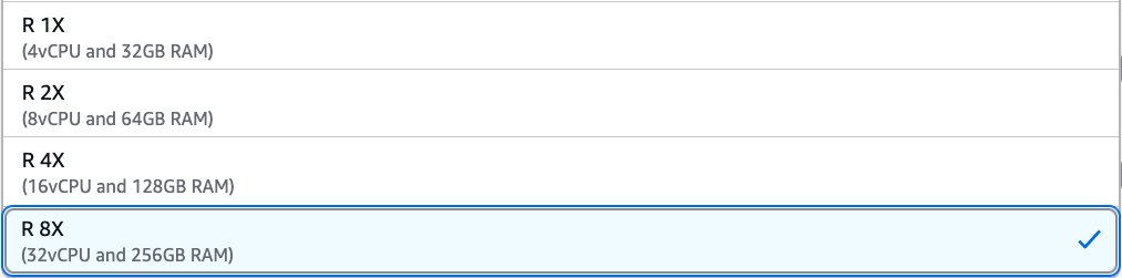
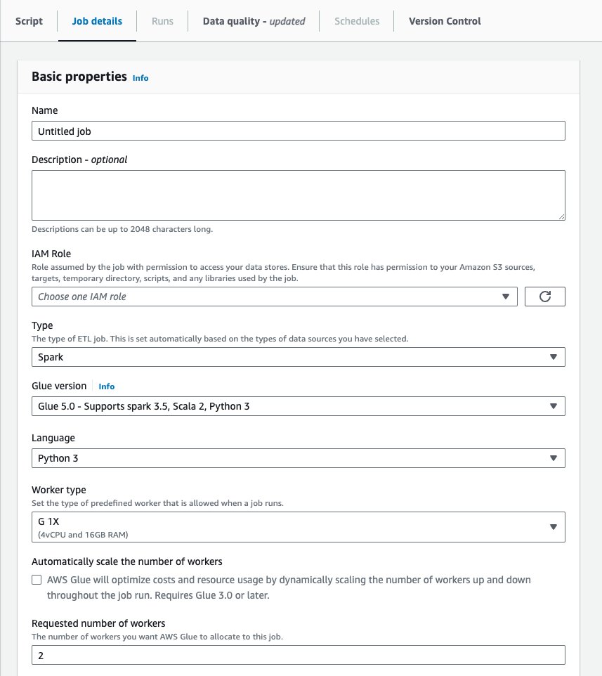
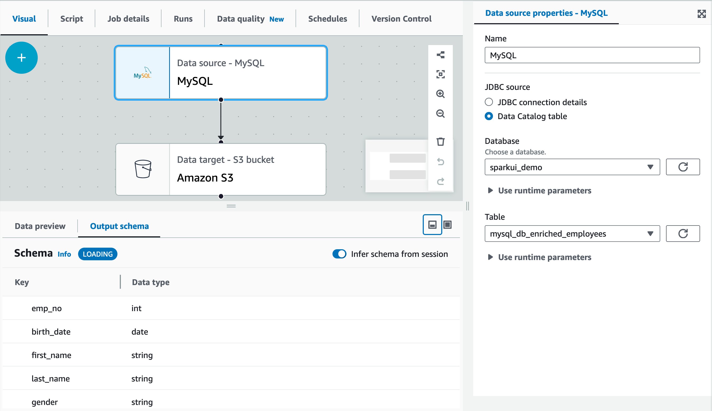
To use R type workers on an AWS Glue job, change the setting of the worker type parameter. In AWS Glue Studio, you can choose R 1X, R 2X, R 4X, or R 8X under Worker type.
In the AWS API or AWS SDK, you can specify R worker types in the WorkerType parameter. In the AWS CLI, you can use the --worker-type parameter in a create-job command.
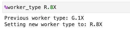
To use R worker types on an AWS Glue Studio notebook or interactive sessions, set R.1X, R.2X, R.4X, or R.8X in the %worker_type magic:
R type workers are priced at $0.52 per DPU-hour for each job, billed per second with a 1-minute minimum.
G.12X and G.16X workers
AWS Glue G.12X and G.16X workers give you more compute, memory, and storage to run your most demanding jobs. G.12X workers provide 12 DPU, with 48 vCPU, 192 GB memory, and 768 GB of disk per worker node. G.16X workers provide 16 DPU, with 64 vCPU, 256 GB memory, and 1024 GB of disk per node. G.16x is double the resources of the existing largest worker type G.8X. You can enable G.12X and G.16X workers with a single parameter change in the API, AWS CLI, or AWS Glue Studio. Regardless of the worker used, the AWS Glue jobs have the same capabilities, including automatic scaling and interactive job authoring using notebooks. G.12X and G.16X workers are available with AWS Glue 4.0 and 5.0.The following table shows compute, memory, disk, and Spark configurations for each G worker type.
| AWS Glue Worker Type | DPU per Node | vCPU | Memory (GB) | Disk (GB) | Approximate Free Disk Space (GB) | Number of Spark Executors per Node | Number of Cores per Spark Executor |
| G.025X | 0.25 | 2 | 4 | 84 | 34 | 1 | 2 |
| G.1X | 1 | 4 | 16 | 94 | 44 | 1 | 4 |
| G.2X | 2 | 8 | 32 | 138 | 78 | 1 | 8 |
| G.4X | 4 | 16 | 64 | 256 | 230 | 1 | 16 |
| G.8X | 8 | 32 | 128 | 512 | 485 | 1 | 32 |
| G.12X (new) | 12 | 48 | 192 | 768 | 741 | 1 | 48 |
| G.16X (new) | 16 | 64 | 256 | 1024 | 996 | 1 | 64 |
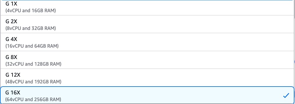
To use G.12X and G.16X workers on an AWS Glue job, change the setting of the worker type parameter to G.12X or G.16X. In AWS Glue Studio, you can choose G 12X or G 16X under Worker type.
In the AWS API or AWS SDK, you can specify G.12X or G.16X in the WorkerType parameter. In the AWS CLI, you can use the --worker-type parameter in a create-job command.
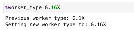
To use G.12X and G.16X on an AWS Glue Studio notebook or interactive sessions, set G.12X or G.16X in the %worker_type magic:
G type workers are priced at $0.44 per DPU-hour for each job, billed per second with a 1-minute minimum. This is the same pricing as the existing worker types.
Choose the right worker type for your workload
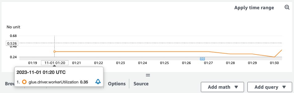
To optimize job resource utilization, run your expected application workload to identify the ideal worker type that aligns with your application’s requirements. Start with general worker types like G.1X or G.2X, and monitor your job run from AWS Glue job metrics, observability metrics, and Spark UI. For more details about how to monitor the resource metrics for AWS Glue jobs, see Best practices for performance tuning AWS Glue for Apache Spark jobs.
When your data processing workload is well distributed across workers, G.1X or G.2X work very well. However, some workloads might require more resources per worker. You can use the new G.12X, G.16X, and R type workers to address them. In this section, we discuss typical use cases where vertical scaling is effective.
Large join operations
Some joins might involve large tables where one or both sides need to be broadcast. Multi-way joins require multiple large datasets to be held in memory. With skewed joins, certain partition keys have disproportionately large data volumes. Horizontal scaling doesn’t help when the entire dataset needs to be in memory on each node for broadcast joins.
High-cardinality group by operations
This use case includes aggregations on columns with many unique values, operations requiring maintenance of large hash tables for grouping, and distinct counts on columns with high uniqueness. High-cardinality operations often result in large hash tables that need to be maintained in memory on each node. Adding more nodes doesn’t reduce the size of these per-node data structures.
Window functions and complex aggregations
Some operations might require a large window frame, or involve computing percentiles, medians, or other rank-based analytics across large datasets, in addition to complex grouping sets or CUBE operations on high-cardinality columns. These operations often require keeping large portions of data in memory per partition. Adding more nodes doesn’t reduce the memory requirement for each individual window or grouping operation.
Complex query plans
Complex query plans can have many stages and deep dependency chains, operations requiring large shuffle buffers, or multiple transformations that need to maintain large intermediate results. These query plans often involve large amounts of intermediate data that need to be held in memory. More nodes don’t necessarily simplify the plan or reduce per-node memory requirements.
Machine learning and complex analytics
With ML and analytics use cases, model training might involve large feature sets, wide transformations requiring substantial intermediate data, or complex statistical computations requiring entire datasets in memory. Many ML algorithms and complex analytics require the entire dataset or large portions of it to be processed together, which can’t be effectively distributed across more nodes.
Data skew scenarios
In some data skew scenarios, you might have to process heavily skewed data where certain partitions are significantly larger, or perform operations on datasets with high-cardinality keys, leading to uneven partition sizes. Horizontal scaling can’t address the fundamental issue of data skew, where some partitions remain much larger than others regardless of the number of nodes.
State-heavy stream processing
State-heavy stream processing can include stateful operations with large state requirements, windowed operations over streaming data with large window sizes, or processing micro-batches with complex state management. Stateful stream processing often requires maintaining large amounts of state per key or window, which can’t be easily distributed across more nodes without compromising the integrity of the state.
In-memory caching
These scenarios might include large datasets that must be be cached for repeated access, iterative algorithms requiring multiple passes over the same data, or caching large datasets for fast access, which often requires keeping substantial portions of data in each node’s memory. Horizontal scaling might not help if the entire dataset needs to be cached on each node for optimal performance.
Data skew example scenarios
Several common patterns can typically cause data skew, such as sorting or groupBy transformations on columns with non-uniformed value distributions, and join operations where certain keys appear more frequently than other keys.
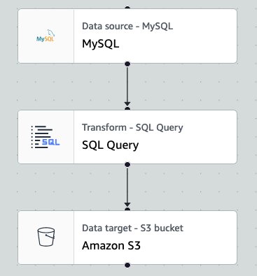
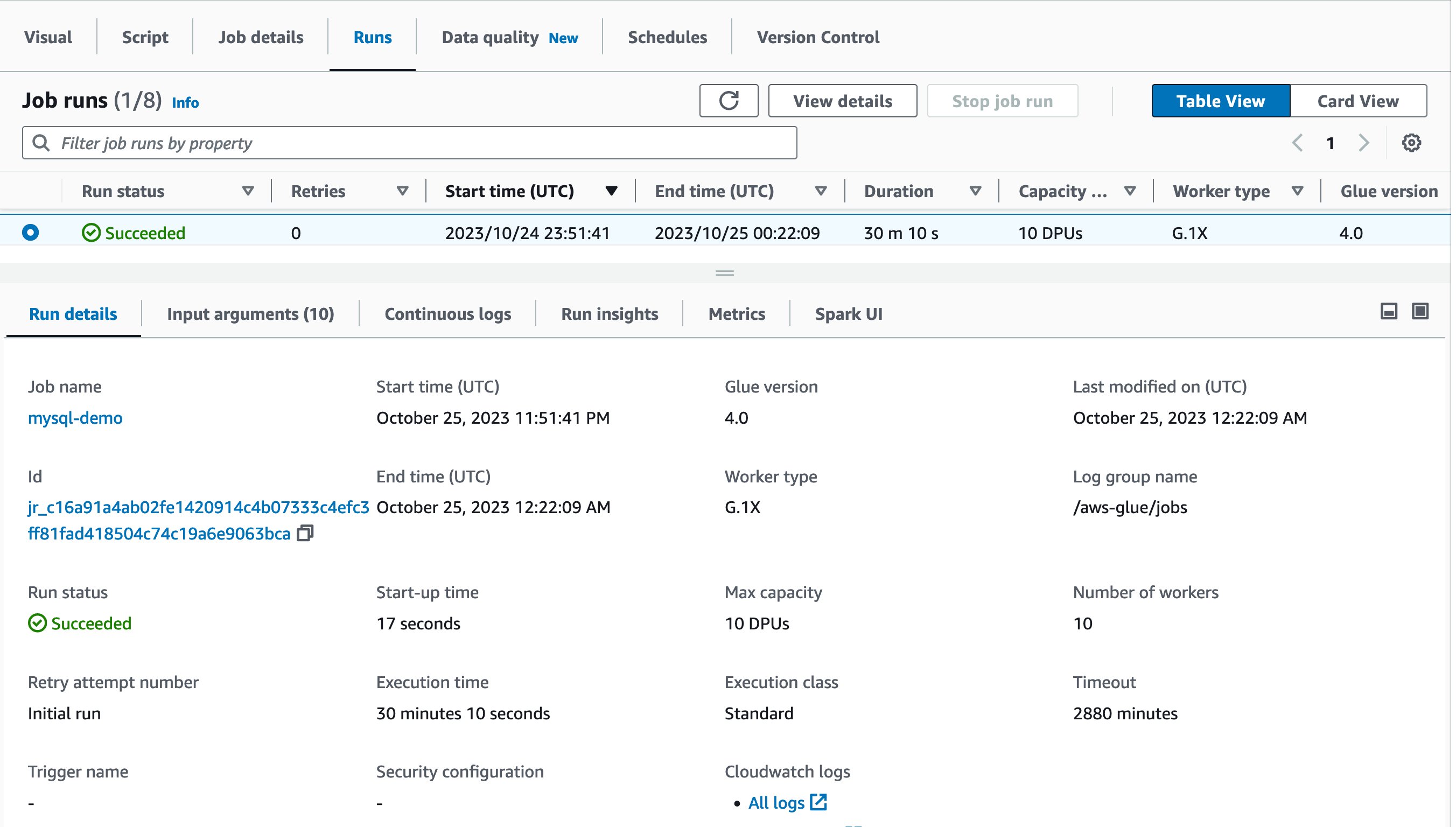
In the following example, we compare the behavior with two different worker types, G.2X and R.2X in the same sample workload to process skewed data.
With G.2X workers
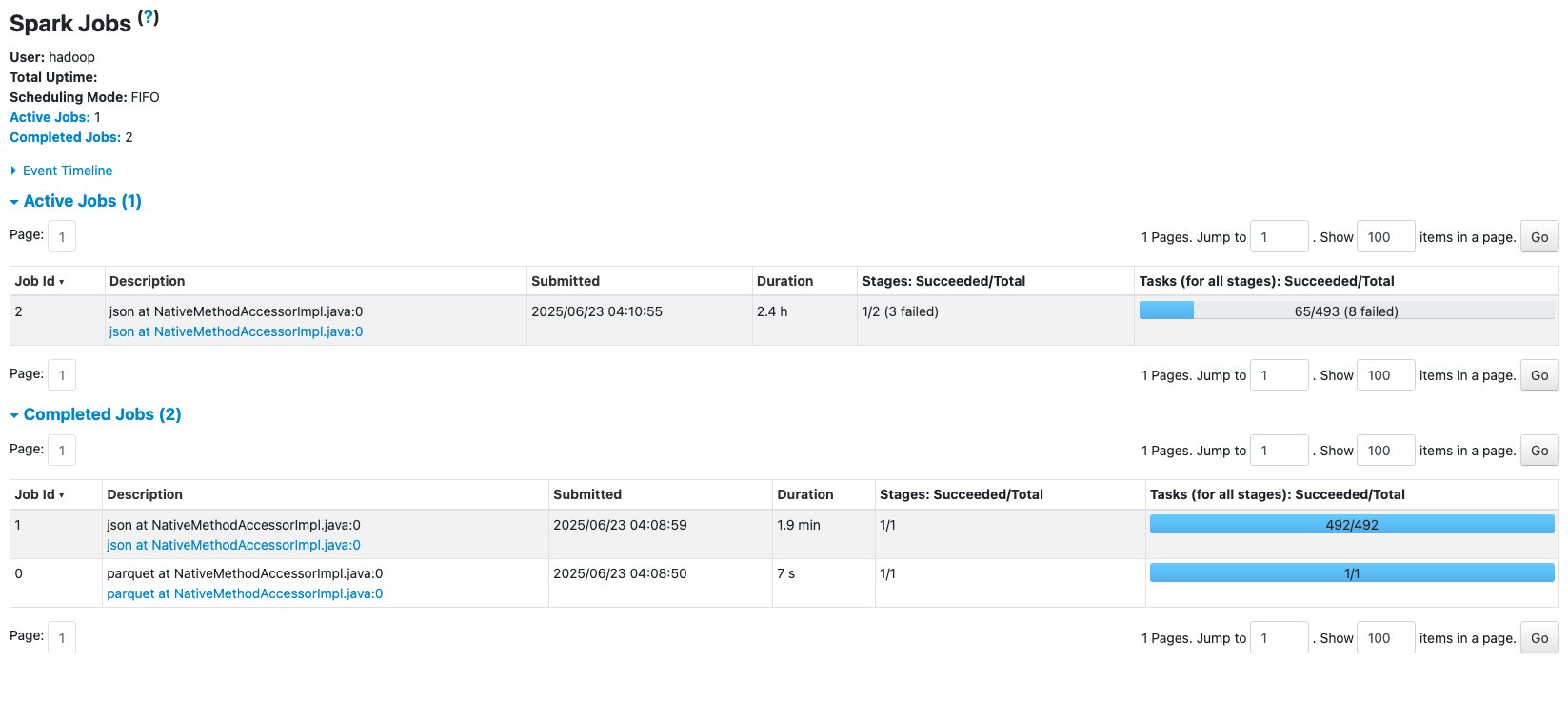
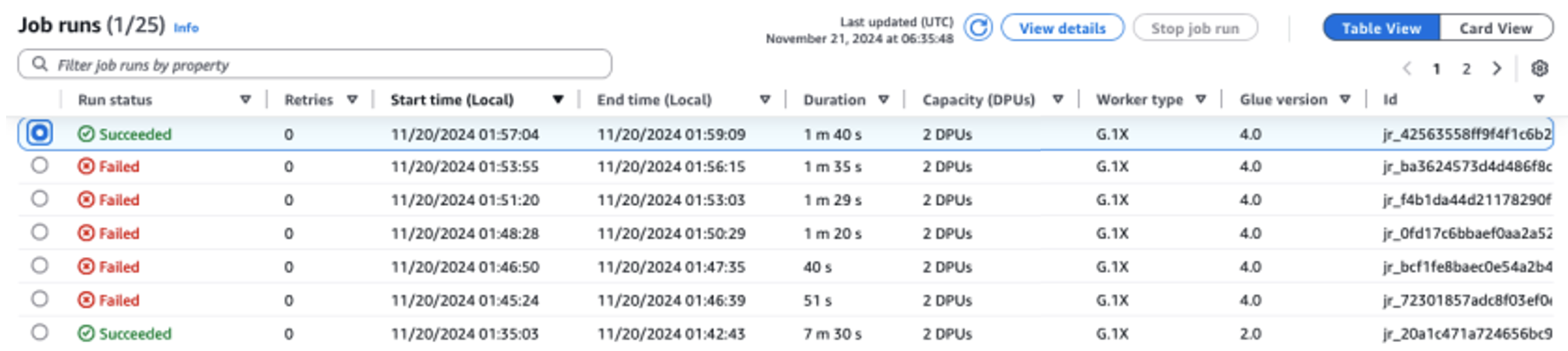
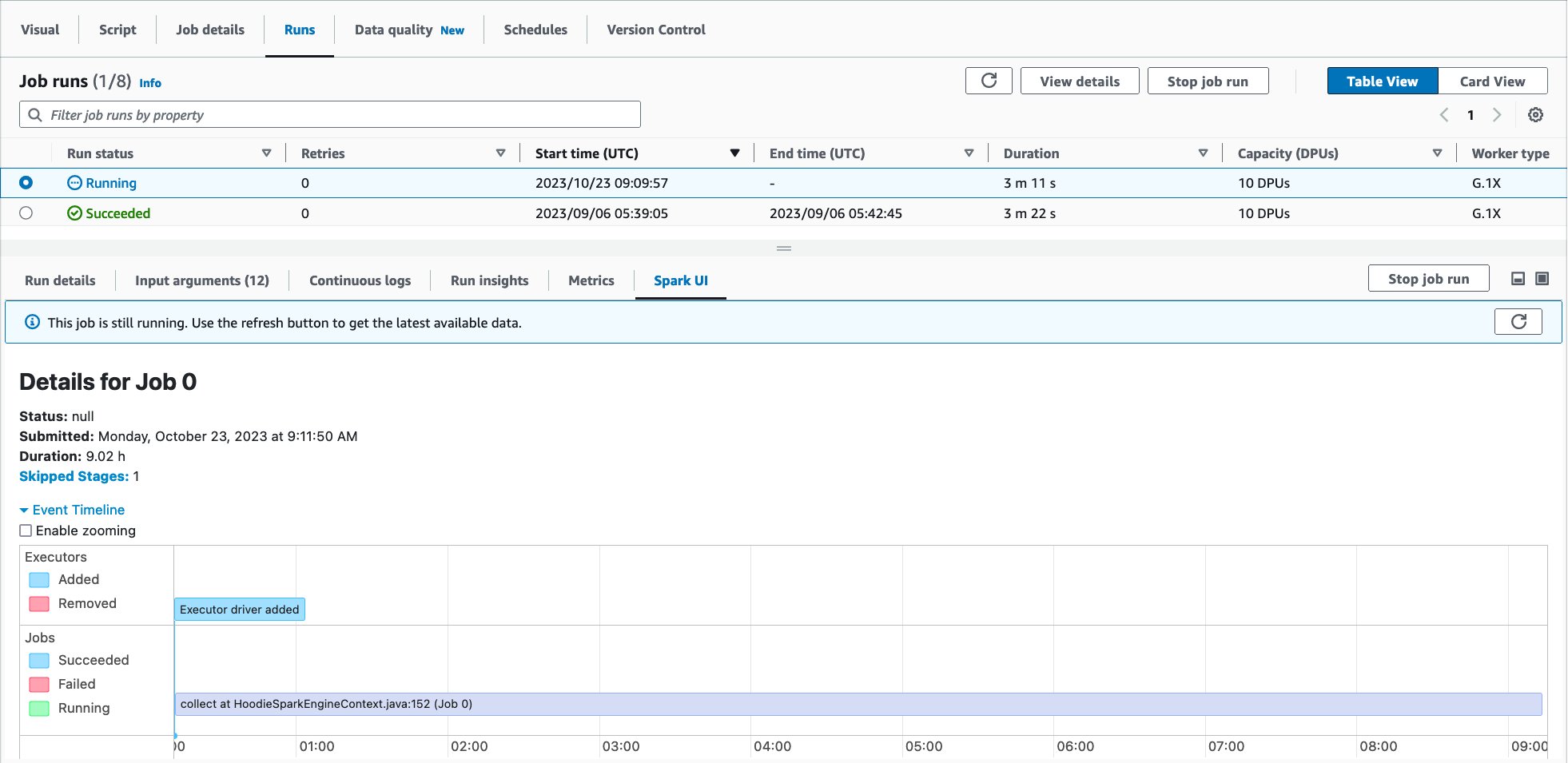
With the G.2X worker type, an AWS Glue job with 10 workers failed due to a No space on left device error while writing records into Amazon Simple Storage Service (Amazon S3). This was mainly caused by large shuffling on a specific column. The following Spark UI view shows the job details.
The Jobs tab shows two completed jobs and one active job where 8 tasks failed out of 493 tasks. Let’s drill down to the details.
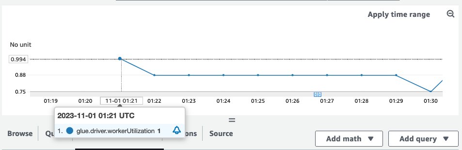
The Executors tab shows an uneven distribution of data processing across the Spark executors, which indicates data skew in this failed job. Executors with IDs 2, 7, and 10 have failed tasks and read approximately 64.5 GiB of shuffle data as shown in the Shuffle Read column. In contrast, the other executors show 0.0 B of shuffle data in the Shuffle Read column.
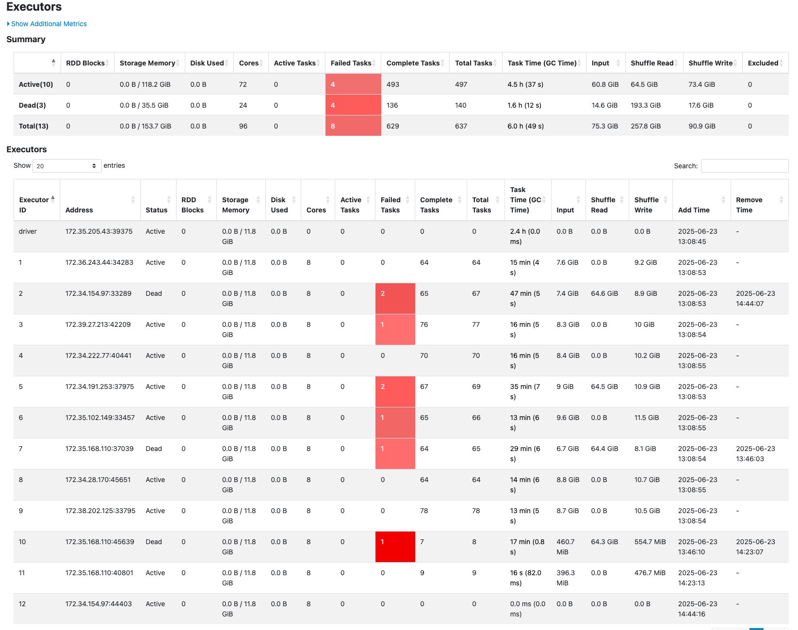
The G.2X worker type can handle most Spark workloads such as data transformations and join operations. However, in this example, there was significant data skew, which caused certain executors to fail due to exceeding the allocated memory.
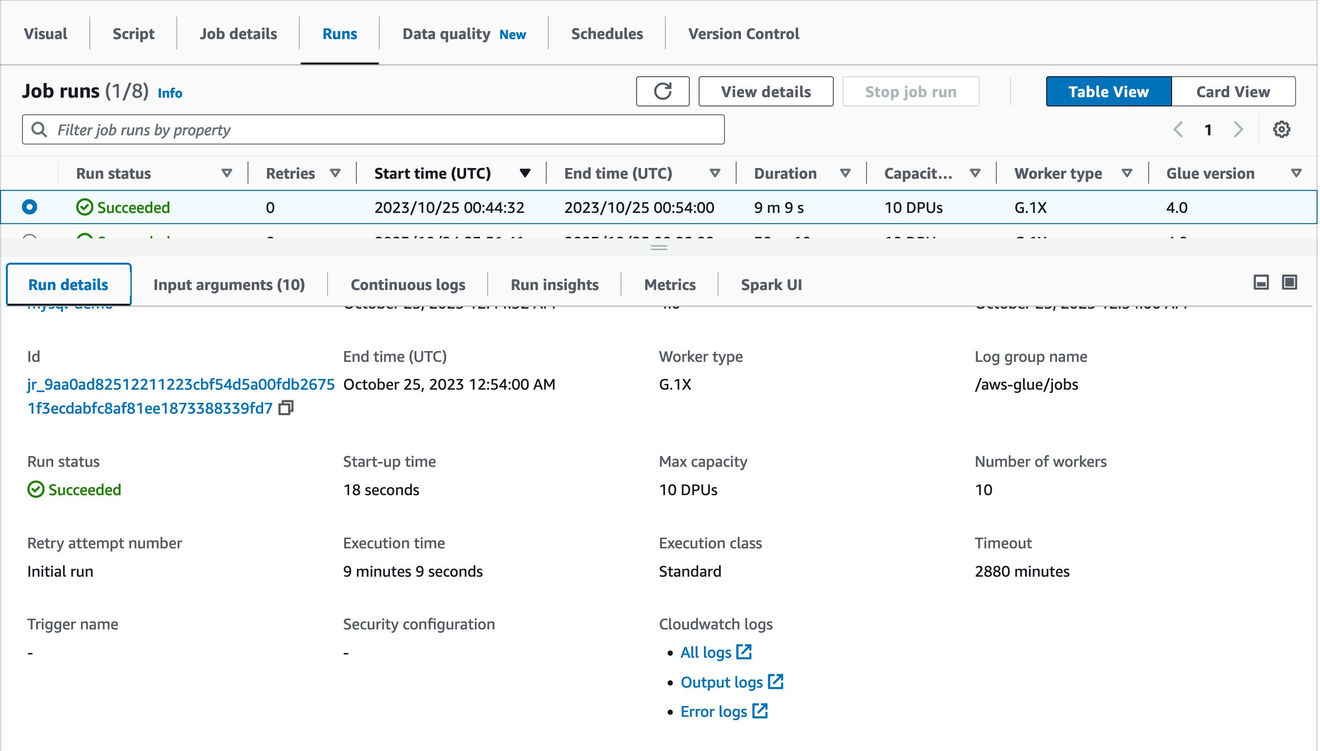
With R.2X workers
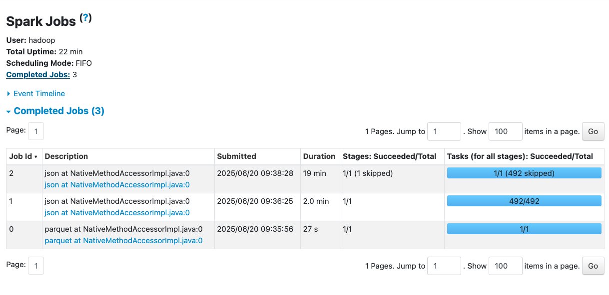
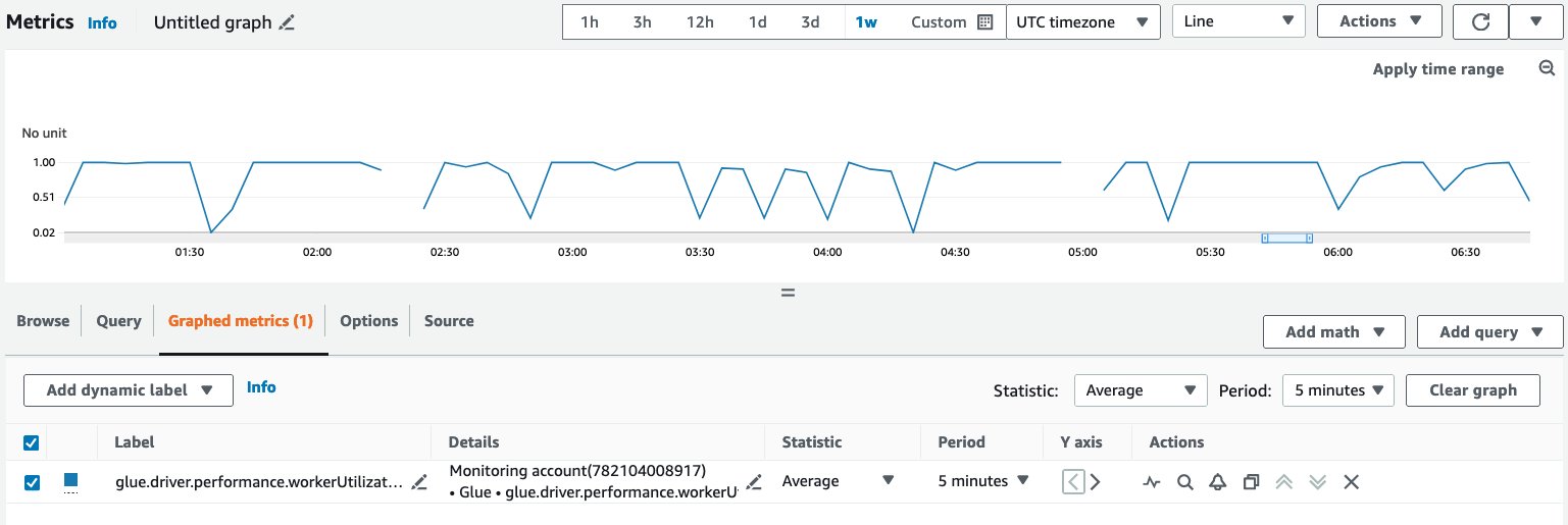
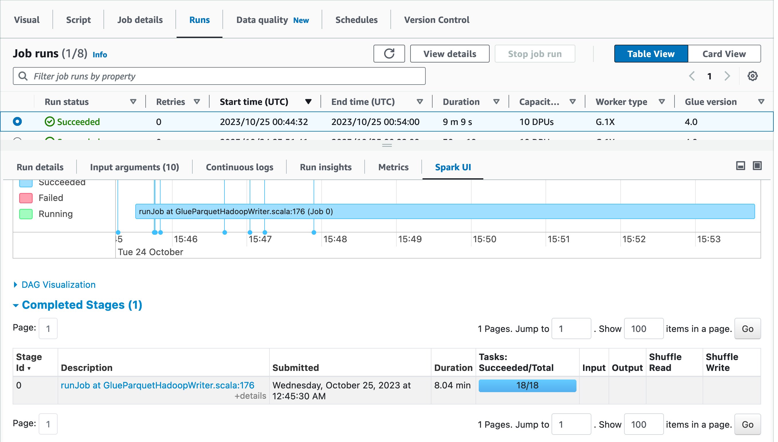
With the R.2X worker type, an AWS Glue job with 10 workers successfully ran without any failures. The number of workers is the same as the previous example—the only difference is the worker type. R workers have two times more memory compared to G workers. The following Spark UI view shows more details.
The Jobs tab shows three completed jobs. No failures are shown on this page.
The Executors tab shows no failed tasks per executor even though there’s an uneven distribution of shuffle reads across executors.
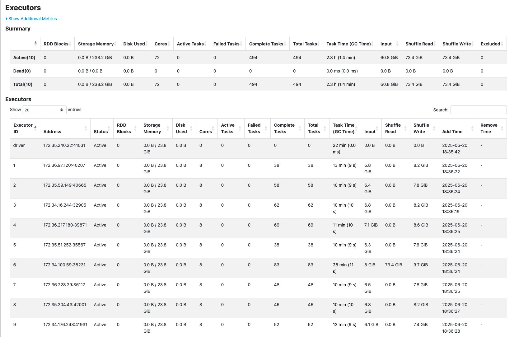
The results showed that R.2X workers successfully completed the workload that failed on G.2X workers using the same number of executors but with the additional memory capacity to handle the skewed data distribution.
Conclusion
In this post, we demonstrated how AWS Glue R type, G.12X, and G.16X workers can help you vertically scale your AWS Glue for Apache Spark jobs. You can start using the new R type, G.12X, and G.16X workers to scale your workload today. For more information on these new worker types and AWS Regions where the new workers are available, visit the AWS Glue documentation.
To learn more, see Getting Started with AWS Glue.
About the Authors
 Noritaka Sekiyama is a Principal Big Data Architect with AWS Analytics services. He’s responsible for building software artifacts to help customers. In his spare time, he enjoys cycling on his road bike.
 Tomohiro Tanaka is a Senior Cloud Support Engineer at Amazon Web Services. He’s passionate about helping customers use Apache Iceberg for their data lakes on AWS. In his free time, he enjoys a coffee break with his colleagues and making coffee at home.
 Peter Tsai is a Software Development Engineer at AWS, where he enjoys solving challenges in the design and performance of the AWS Glue runtime. In his leisure time, he enjoys hiking and cycling.
 Matt Su is a Senior Product Manager on the AWS Glue team. He enjoys helping customers uncover insights and make better decisions using their data with AWS Analytics services. In his spare time, he enjoys skiing and gardening.
 Sean McGeehan is a Software Development Engineer at AWS, where he builds features for the AWS Glue fulfillment system. In his leisure time, he explores his home of Philadelphia and work city of New York.


 Stefano Sandonà is a Senior Big Data Specialist Solution Architect at Amazon Web Services (AWS). Passionate about data, distributed systems, and security, he helps customers worldwide architect high-performance, efficient, and secure data solutions.
 Derek Liu is a Senior Solutions Architect based out of Vancouver, BC. He enjoys helping customers solve big data challenges through Amazon Web Services (AWS) analytic services.
 Raj Ramasubbu is a Senior Analytics Specialist Solutions Architect focused on big data and analytics and AI/ML with Amazon Web Services (AWS). He helps customers architect and build highly scalable, performant, and secure cloud-based solutions on AWS. Raj provided technical expertise and leadership in building data engineering, big data analytics, business intelligence, and data science solutions for over 18 years prior to joining AWS. He helped customers in various industry verticals like healthcare, medical devices, life science, retail, asset management, car insurance, residential REIT, agriculture, title insurance, supply chain, document management, and real estate.
 Angel Conde Manjon is a Sr. EMEA Data & AI PSA, based in Madrid. He has previously worked on research related to data analytics and AI in diverse European research projects. In his current role, Angel helps partners develop businesses centered on data and AI.


 Noritaka Sekiyama is a Principal Big Data Architect for AWS Analytics services with a strong focus on data engineering. He is responsible for building software artifacts to help customers. In his spare time, he enjoys cycling on his road bike.
 Daniel Obi is a Frontend Engineer on the Amazon SageMaker Unified Studio team. He is dedicated to building intuitive and effective solutions that enhance user experience and technical functionality. Outside of his professional work, he enjoys watching and playing basketball.
 Vasudevan Venkataramanan is a Senior Software Engineer on the Amazon SageMaker Unified Studio team. He is responsible for technical direction of scheduling and orchestration within SageMaker Unified Studio. Outside of his professional work, he enjoys spending time with his kid, and playing pickleball and cricket.
 Yuhang Huang is a Software Development Manager on the Amazon SageMaker Unified Studio team. He leads the engineering team to design, build, and operate scheduling and orchestration capabilities in SageMaker Unified Studio. In his free time, he enjoys playing tennis.
 Gal Heyne is a Senior Technical Product Manager for AWS Analytics services with a strong focus on AI/ML and data engineering. She is passionate about developing a deep understanding of customers’ business needs and collaborating with engineers to design simple-to-use data products.


 Chiho Sugimoto is a Cloud Support Engineer on the AWS Big Data Support team. She is passionate about helping customers build data lakes using ETL workloads. She loves planetary science and enjoys studying the asteroid Ryugu on weekends.
 Zach Mitchell is a Sr. Big Data Architect. He works within the product team to enhance understanding between product engineers and their customers while guiding customers through their journey to develop data lakes and other data solutions on AWS analytics services.
 Chanu Damarla is a Principal Product Manager on the Amazon SageMaker Unified Studio team. He works with customers around the globe to translate business and technical requirements into products that delight customers and enable them to be more productive with their data, analytics, and AI.


 Stuti Deshpande is a Big Data Specialist Solutions Architect at AWS. She works with customers around the globe, providing them strategic and architectural guidance on implementing analytics solutions using AWS. She has extensive experience in big data, ETL, and analytics. In her free time, Stuti likes to travel, learn new dance forms, and enjoy quality time with family and friends.
 Martin Ma is a Software Development Engineer on the AWS Glue team. He is passionate about improving the customer experience by applying problem-solving skills to invent new software solutions, as well as constantly searching for ways to simplify existing ones. In his spare time, he enjoys singing and playing the guitar.
 Anshul Sharma is a Software Development Engineer in AWS Glue Team.
 Rajendra Gujja is a Software Development Engineer on the AWS Glue team. He is passionate about distributed computing and everything and anything about data.
 Maheedhar Reddy Chappidi is a Sr. Software Development Engineer on the AWS Glue team. He is passionate about building fault tolerant and reliable distributed systems at scale. Outside of his work, Maheedhar is passionate about listening to podcasts and playing with his two-year-old kid.
 Savio Dsouza is a Software Development Manager on the AWS Glue team. His team works on generative AI applications for the Data Integration domain and distributed systems for efficiently managing data lakes on AWS and optimizing Apache Spark for performance and reliability.
 Kartik Panjabi is a Software Development Manager on the AWS Glue team. His team builds generative AI features for the Data Integration and distributed system for data integration.
 Mohit Saxena is a Senior Software Development Manager on the AWS Glue and Amazon EMR team. His team focuses on building distributed systems to enable customers with simple-to-use interfaces and AI-driven capabilities to efficiently transform petabytes of data across data lakes on Amazon S3, and databases and data warehouses on the cloud.


 Noritaka Sekiyama is a Principal Big Data Architect on the AWS Glue team. He is responsible for building software artifacts to help customers. In his spare time, he enjoys cycling with his road bike.
 Vishal Kajjam is a Software Development Engineer on the AWS Glue team. He is passionate about distributed computing and using ML/AI for designing and building end-to-end solutions to address customers’ data integration needs. In his spare time, he enjoys spending time with family and friends.
 Shubham Mehta is a Senior Product Manager at AWS Analytics. He leads generative AI feature development across services such as AWS Glue, Amazon EMR, and Amazon MWAA, using AI/ML to simplify and enhance the experience of data practitioners building data applications on AWS.
 Wei Tang is a Software Development Engineer on the AWS Glue team. She is strong developer with deep interests in solving recurring customer problems with distributed systems and AI/ML.
 XiaoRun Yu is a Software Development Engineer on the AWS Glue team. He is working on building new features for AWS Glue to help customers. Outside of work, Xiaorun enjoys exploring new places in the Bay Area.
 Jake Zych is a Software Development Engineer on the AWS Glue team. He has deep interest in distributed systems and machine learning. In his spare time, Jake likes to create video content and play board games.
 Savio Dsouza is a Software Development Manager on the AWS Glue team. His team works on distributed systems & new interfaces for data integration and efficiently managing data lakes on AWS.


 Keerthi Chadalavada is a Senior Software Development Engineer at AWS Glue, focusing on combining generative AI and data integration technologies to design and build comprehensive solutions for customers’ data and analytics needs.
 Pradeep Patel is a Software Development Manager on the AWS Glue team. He is passionate about helping customers solve their problems by using the power of the AWS Cloud to deliver highly scalable and robust solutions. In his spare time, he loves to hike and play with web applications.
 Chuhan Liu is a Software Engineer at AWS Glue. He is passionate about building scalable distributed systems for big data processing, analytics, and management. He is also keen on using generative AI technologies to provide brand-new experience to customers. In his spare time, he likes sports and enjoys playing tennis.
 Vaibhav Naik is a software engineer at AWS Glue, passionate about building robust, scalable solutions to tackle complex customer problems. With a keen interest in generative AI, he likes to explore innovative ways to develop enterprise-level solutions that harness the power of cutting-edge AI technologies.


 Paul Villena is an Analytics Solutions Architect in AWS with expertise in building modern data and analytics solutions to drive business value. He works with customers to help them harness the power of the cloud. His areas of interest are infrastructure as code, serverless technologies, and coding in Python.
 Justin Lin is a software engineer on the AWS Lake Formation team. He works on delivering managed optimization solutions for open table formats to enhance customer data management and query performance. In his spare time, he enjoys playing tennis.
 Himani Desai is a Software Engineer on the AWS Lake Formation team. She works on providing managed optimization solutions for Iceberg tables.
 Abishek Shankar is a software engineer on the AWS Lake Formation team, working on providing managed optimization solutions for Iceberg tables.
 Shyam Rathi is a Software Development Manager on the AWS Lake Formation team, working on delivering new features and enhancements related to modern data lakes.
 Sandeep Adwankar is a Senior Product Manager at AWS. Based in the California Bay Area, he works with customers around the globe to translate business and technical requirements into products that enable customers to improve how they manage, secure, and access data.


 Gyan Radhakrishnan is a Software Development Engineer on the AWS Glue team. He is working on designing and building end-to-end solutions for data intensive applications.
 Simon Kern is a Software Development Engineer on the AWS Glue team. He is enthusiastic about serverless technologies, data engineering and building great services.
 Dana Adylova is a Software Development Engineer on the AWS Glue team. She is working on building software for supporting data intensive applications. In her spare time, she enjoys knitting and reading sci-fi.


 Vaibhav Porwal is a Senior Software Development Engineer on the AWS Glue and AWS Data Pipeline team. He is working on solving problems in orchestration space by building low cost, repeatable, scalable workflow systems that enables customers to create their ETL pipelines seamlessly.
 Sriram Ramarathnam is a Software Development Manager on the AWS Glue and AWS Data Pipeline team. His team works on solving challenging distributed systems problems for data integration across AWS serverless and serverfull compute offerings.


 Gonzalo Herreros is a Senior Big Data Architect on the AWS Glue team, with a background in machine learning and AI.


 Sean Ma is a Principal Product Manager on the AWS Glue team. He has a track record of more than 18 years innovating and delivering enterprise products that unlock the power of data for users. Outside of work, Sean enjoys scuba diving and college football.


 Xiaoxi Liu is a Software Development Engineer on the AWS Glue team. Her passion is building scalable distributed systems for efficiently managing big data on the cloud, and her concentrations are distributed system, big data, and cloud computing.
 Akira Ajisaka is a Senior Software Development Engineer on the AWS Glue team. He likes open source software and distributed systems. In his spare time, he enjoys playing arcade games.
 Shenoda Guirguis is a Senior Software Development Engineer on the AWS Glue team. His passion is in building scalable and distributed data infrastructure and processing systems. When he gets a chance, Shenoda enjoys reading and playing soccer.


 Kinshuk Pahare is a leader in AWS Glue’s product management team. He drives efforts on the platform, developer experience, and big data processing frameworks like Apache Spark, Ray, and Python Shell.


 Benjamin Menuet is a Senior Data Architect on the AWS Professional Services team at Amazon Web Services. He helps customers develop data and analytics solutions to accelerate their business outcomes. Outside of work, Benjamin is a trail runner and has finished some iconic races like the UTMB.
 Akira Ajisaka is a Senior Software Development Engineer on the AWS Glue team. He likes open source software and distributed systems. In his spare time, he enjoys playing arcade games.
 Jason Ganz is the manager of the Developer Experience (DX) team at dbt Labs


 Kyle Duong is a Software Development Engineer on the AWS Glue and Lake Formation team. He is passionate about building big data technologies and distributed systems.
 Sandeep Adwankar is a Senior Technical Product Manager at AWS. Based in the California Bay Area, he works with customers around the globe to translate business and technical requirements into products that enable customers to improve how they manage, secure, and access data.

 Alexandra Tello is a Senior Front End Engineer with the AWS Glue team in New York City. She is a passionate advocate for usability and accessibility. In her free time, she’s an espresso enthusiast and enjoys building mechanical keyboards.
 Matt Sampson is a Software Development Manager on the AWS Glue team. He loves working with his other Glue team members to make services that our customers benefit from. Outside of work, he can be found fishing and maybe singing karaoke.


