All posts by Raj Ramasubbu

Build stateful streaming applications with Apache Spark 4.0 on Amazon EMR Serverless

Post Syndicated from Raj Ramasubbu original https://aws.amazon.com/blogs/big-data/build-stateful-streaming-applications-with-apache-spark-4-0-on-amazon-emr-serverless/

Apache Spark 4.0 represents a major milestone in stream processing, introducing new capabilities that fundamentally change how developers build stateful streaming applications. At the heart of these improvements is the transformWithState API – a new capability that enables first-class support for timers, automatic state management, and schema evolution to Spark Structured Streaming.

With Spark 4.0 now available on Amazon EMR Serverless, developers can build stateful streaming applications using the transformWithState API in a fully managed, serverless environment that automatically scales based on workload demands. This combination delivers the power of sophisticated stream processing without the operational overhead of cluster management.

In this post, we demonstrate how to build a production-ready IoT device monitoring system using Spark 4.0’s transformWithState API on Amazon EMR Serverless. This example showcases the key capabilities of stateful streaming and provides a template you can adapt for your own use cases.

Apache Spark 4.0: introducing transformWithState

Apache Spark 4.0’s latest streaming features solve common production challenges in stateful applications by introducing native timer support and advance state management capabilities for complex event processing workflows. The new transformWithState API provides:

Key features of transformWithState

  • Native timer support: Register timers that fire callbacks at specific times for use cases like heartbeat monitoring, session timeout detection, and SLA violation alerts.
  • Automatic state TTL (Time-To-Live): Configure automatic expiration policies to prevent state from growing indefinitely. This is useful for use cases like session state size control, clearing stale device telemetry, maintaining a recency cache, or tracking invalid logins within the last hour for fraud detection.
  • Schema evolution: Evolve state schema without restarting from a new checkpoint. Add optional fields, remove fields, or widen numeric types. This is particularly valuable for use cases where data structures are dynamic, and application downtime for schema migration is not acceptable, enabling more resilient and flexible real-time streaming applications.
  • Multiple state variables: Support for multiple independent state variables (ValueState, ListState, MapState) per key, well-suited for building complex, real-time applications that require sophisticated state management, such as storing a history of recent error codes, tracking counts of various alert types, or maintaining multiple dimensions of user activity within a single stateful operator.
  • State observability: Query application state mid-stream using the State Data Source Reader for debugging and monitoring. This is especially valuable in applications that require maintaining and evolving state through several steps, such as detection of sophisticated event patterns across multiple streams and over time, where visibility into state transitions is critical for troubleshooting and validation.
  • Operator chaining: Chain multiple stateful operators together for complex multi-stage processing pipelines.

These capabilities make Spark 4.0 ideal for applications that were previously difficult or impossible to implement efficiently, such as complex event processing, session analytics, anomaly detection, and real-time monitoring systems.

Use case: IoT heartbeat monitoring

Consider a fleet of 100,000 IoT sensors deployed across manufacturing facilities. Each sensor sends a heartbeat signal every 20 seconds to indicate it’s operational. Your operations team needs to be alerted within 30 seconds if any sensor goes offline, with repeat alerts every 60 seconds until the sensor comes back online.

This seemingly simple requirement presents several technical challenges. The application must maintain the last heartbeat timestamp for each of the 100,000 devices while independently managing timers to detect missed signals per device. It also needs to handle out-of-order heartbeats caused by network delays and clean up state for decommissioned devices to prevent unbounded memory growth. All of this must happen at scale, processing millions of events per minute with low latency, while recovering gracefully from failures without losing state.

To address the specific challenges of IoT heartbeat monitoring described above, we present a solution built on the transformWithState API in Spark 4.0. With its native timer support, automatic state management, and built-in fault tolerance, making it the ideal solution for IoT heartbeat monitoring at scale.

Solution overview

Our solution architecture follows a serverless, event-driven design:
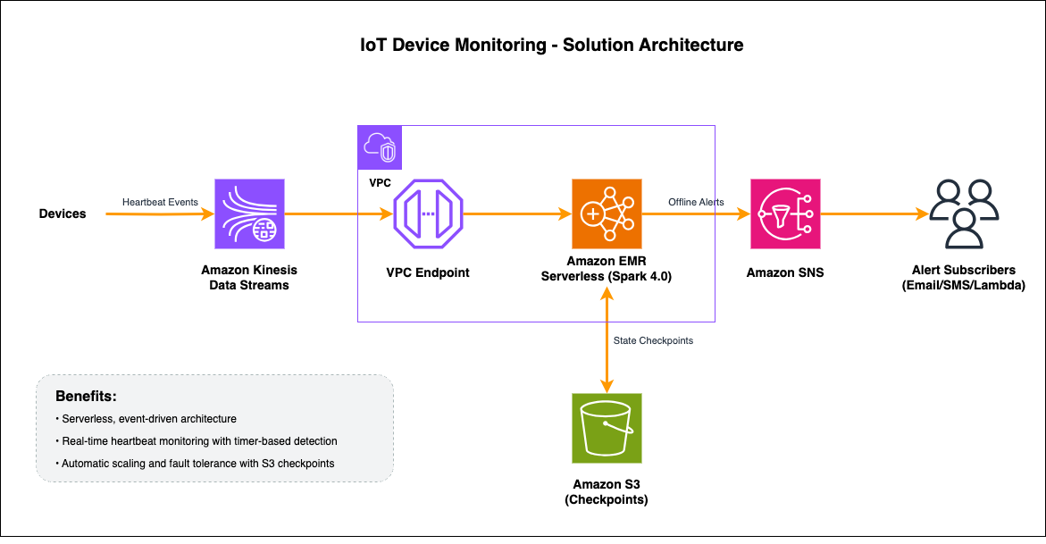
Solution architecture showing IoT devices sending heartbeats to Kinesis Data Streams, processed by EMR Serverless with transformWithState, checkpointed to Amazon S3, and alerts delivered via Amazon SNS

  1. IoT devices send heartbeat events to Amazon Kinesis Data Streams containing device ID, timestamp, and metadata (battery level, signal strength, firmware version).
  2. Amazon EMR Serverless reads from Kinesis using the Spark aws-kinesis connector using VPC Endpoint for Kinesis, then parses JSON events into structured DataFrames and grouping by device_id.
  3. transformWithState processes each device’s stream. On heartbeat arrival, it updates state and registers a 30-second timer; when the timer expires without a new heartbeat, it emits an offline alert.
  4. State is automatically persisted to RocksDB locally and checkpointed to Amazon Simple Storage Service (Amazon S3), enabling fault-tolerant recovery and exactly-once processing semantics.
  5. Alerts are delivered via Amazon Simple Notification Service (Amazon SNS) to configured subscribers (email, SMS, AWS Lambda, webhooks).

Prerequisites

Before implementing this solution, verify that you have:

  1. AWS account: With permissions for EMR Serverless, Kinesis, SNS, S3, VPC, and IAM.
  2. AWS Command Line Interface (AWS CLI): Configured with appropriate credentials.
  3. VPC setup: VPC with private subnets and security groups configured.
  4. Kinesis VPC interface endpoint: VPC endpoint for private connectivity to Kinesis.
  5. Kinesis Data Stream: Created for ingesting heartbeat events (for example, iot-heartbeats). For testing your streaming data solution, refer to Test your streaming data solution with the new Amazon Kinesis Data Generator.
  6. SNS topic: Created for sending alerts (for example, iot-alerts).
  7. S3 bucket: For storing application code, dependencies, and checkpoints.

Step-by-step implementation

The following steps walk you through setting up an EMR Serverless application with Spark 4.0, configuring the stateful streaming processor, and deploying the IoT heartbeat monitoring solution.

Step 1: Create the EMR serverless application

Run the following command in your terminal using the AWS CLI. Replace the subnet and security group IDs with the values from your VPC setup.

# Create EMR Serverless application with Spark 4.0 and VPC
aws emr-serverless create-application \
  --name "iot-heartbeat-monitor" \
  --release-label "emr-spark-8.0.0" \
  --type "SPARK" \
  --network-configuration '{
    "subnetIds": ["subnet-xxxxx", "subnet-yyyyy"],
    "securityGroupIds": ["sg-zzzzz"]
  }' \
  --region us-east-1

The command returns a JSON response containing the application details. Note the applicationId value from the output, as you will need it in subsequent steps.

Step 2: Implement the heartbeat monitor

The core of our solution is the HeartbeatMonitor class that extends StatefulProcessor. This class demonstrates the key features of Spark 4.0’s transformWithState API. Download the full implementation script and upload it to your local S3 bucket for execution. Let’s walk through each component to understand how it works.

2.1 Initialize state variables

The init() method is called once when the processor is initialized. This is where we define and register our state variables.

from pyspark.sql.streaming.stateful_processor import (
    StatefulProcessor, StatefulProcessorHandle
)

class HeartbeatMonitor(StatefulProcessor):

    def init(self, handle: StatefulProcessorHandle) -> None:
        self.handle = handle

        # Define state schemas
        last_seen_schema = StructType([
            StructField("timestamp", TimestampType(), True)
        ])

        device_info_schema = StructType([
            StructField("battery_level", StringType(), True),
            StructField("firmware_version", StringType(), True)
        ])

        # Initialize multiple independent state variables
        self.last_seen = handle.getValueState("last_seen", last_seen_schema)
        self.device_info = handle.getValueState(
            "device_info", device_info_schema
        )

In the init() method, we use StatefulProcessorHandle to define and initialize two per-key state variables, last_seen and device_info, using Spark’s StructType schemas and the getValueState() API. These state variables are automatically stored in RocksDB and checkpointed to S3, allowing for fault-tolerant state management across streaming micro-batches.

2.2 Handle incoming heartbeat events and register timers

The handleInputRows() method is called whenever new events arrive for a device. This is where we update state and register timers.

def handleInputRows(
    self, key: tuple, rows: Iterator[pd.DataFrame], timerValues
) -> Iterator[pd.DataFrame]:
    device_id = key[0]

    # Process incoming heartbeats - iterate through all rows to find latest
    latest_timestamp = None
    for pdf in rows:
        for _, row in pdf.iterrows():
            ts = row['timestamp']
            if pd.isna(ts):
                continue
            if latest_timestamp is None or ts > latest_timestamp:
                latest_timestamp = ts

    if latest_timestamp is None:
        yield pd.DataFrame()
        return

    # Check if we have existing state
    existing_timestamp = None
    if self.last_seen.exists():
        existing_state = self.last_seen.get()
        existing_timestamp = existing_state[0]

    # Update state only if new heartbeat is more recent
    if existing_timestamp is None or latest_timestamp > existing_timestamp:
        # Cancel existing timers (device is back online)
        for timer in self.handle.listTimers():
            self.handle.deleteTimer(timer)

        # Update state with new timestamp
        self.last_seen.update((latest_timestamp,))

        # Register timer for heartbeat deadline detection
        current_time_ms = timerValues.getCurrentProcessingTimeInMs()
        deadline_ms = current_time_ms + HEARTBEAT_INTERVAL_MS
        # 30 seconds from now
        self.handle.registerTimer(deadline_ms)

    yield pd.DataFrame()  # No output from input handling

The handleInputRows() method processes incoming heartbeat events for each device by extracting the latest timestamp, updating the last_seen state, and managing timers. It cancels existing ones and registering a new 30-second expiry timer to detect future inactivity. Because alerts are only emitted upon timer expiration, the method yields an empty dataframe during normal heartbeat processing.

2.3 Handle timer expiration and emit alerts

The handleExpiredTimer() method is called when a registered timer fires. This is where we detect offline devices and emit alerts.

def handleExpiredTimer(
    self, key: tuple, timerValues, expiredTimerInfo
) -> Iterator[pd.DataFrame]:
    device_id = key[0]
    current_time_ms = timerValues.getCurrentProcessingTimeInMs()

    # Verify state exists
    if not self.last_seen.exists():
        yield pd.DataFrame()
        return

    # Get last seen timestamp from state
    last_seen_state = self.last_seen.get()
    last_seen_timestamp = last_seen_state[0]

    if last_seen_timestamp is None or pd.isna(last_seen_timestamp):
        yield pd.DataFrame()
        return

    # Calculate how long device has been offline
    last_seen_ms = int(last_seen_timestamp.timestamp() * 1000)
    offline_duration_ms = current_time_ms - last_seen_ms
    offline_duration_seconds = offline_duration_ms / 1000.0

    # Create alert as a Pandas DataFrame
    alert_df = pd.DataFrame({
        "device_id": [device_id],
        "alert_type": ["DEVICE_OFFLINE"],
        "last_seen": [last_seen_timestamp],
        "offline_duration_seconds": [offline_duration_seconds],
        "alert_timestamp": [datetime.fromtimestamp(current_time_ms / 1000.0)]
    })

    # Register another timer for repeat alerts (every 60 seconds)
    next_alert_time = current_time_ms + ALERT_REPEAT_INTERVAL_MS
    self.handle.registerTimer(next_alert_time)

    yield alert_df  # Emit the alert

The handleExpiredTimer() method is triggered automatically when a device’s inactivity timer expires, retrieving the last_seen state to calculate the offline duration and yielding an alert dataframe to the output stream. It also registers a follow-up timer for repeat alerts every 60 seconds, which continues until a new heartbeat arrives and cancels the timer via handleInputRows().

There are several ways you could extend this solution for production use. You could implement exponential backoff for repeat alerts to reduce noise, for example, alerting after 60 seconds, then 2 minutes, then 5 minutes, and so on. Other improvements could include adding severity escalation based on offline duration, integrating with notification services like Amazon SNS for downstream alerting, or setting a maximum retry limit to stop alerts for permanently decommissioned devices.

2.4 Apply transformWithState to the streaming DataFrame

Now we connect everything together by applying our HeartbeatMonitor processor to the streaming data.

# Read and parse heartbeat events from Kinesis
parsed_df = kinesis_df \
    .selectExpr("CAST(data AS STRING) as json_data") \
    .select(from_json(col("json_data"), heartbeat_schema).alias("heartbeat")) \
    .select(
        col("heartbeat.device_id"),
        to_timestamp(col("heartbeat.timestamp")).alias("timestamp"),
        col("heartbeat.battery_level"),
        col("heartbeat.signal_strength"),
        col("heartbeat.firmware_version")
    )

# Apply transformWithState for stateful processing
alerts_df = parsed_df \
    .groupBy("device_id") \
    .transformWithStateInPandas(
        statefulProcessor=HeartbeatMonitor(),
        outputStructType=alert_output_schema,
        outputMode="append",
        timeMode="processingTime"
    )

# Write alerts to SNS
query = alerts_df.writeStream \
    .outputMode("append") \
    .foreachBatch(send_to_sns) \
    .option("checkpointLocation", CHECKPOINT_LOCATION) \
    .trigger(processingTime="10 seconds") \
    .start()

# Send to SNS for alerts
def send_to_sns(batch_df, batch_id):
    if batch_df.count() > 0:
        sns_client = boto3.client('sns', region_name=KINESIS_REGION)
        for row in batch_df.collect():
            message = {
                "device_id": row["device_id"],
                "alert_type": row["alert_type"],
                "last_seen": str(row["last_seen"]),
                "offline_duration_seconds": row["offline_duration_seconds"],
                "alert_timestamp": str(row["alert_timestamp"])
            }
            sns_client.publish(
                TopicArn=SNS_TOPIC_ARN,
                Message=json.dumps(message),
                Subject=f"Device Offline Alert: {row['device_id']}"
            )

The streaming pipeline parses JSON heartbeat events from Kinesis, partitions them by device_id, and applies the HeartbeatMonitor stateful processor using transformWithStateInPandas() with processing-time timers and append output mode. The resulting alert stream is written to SNS via foreachBatch() with checkpointing enabled for fault tolerance and micro-batches triggered every 10 seconds.

To summarize, implementing the heartbeat monitor requires just three methods. The init() method sets up your state variables, handleInputRows() processes incoming heartbeats and manages timers, and handleExpiredTimer() generates offline alerts. The transformWithState API handles the underlying complexity of state management, checkpointing, and timer scheduling automatically.

Step 3: Create IAM role for job execution

Create an IAM role that allows EMR Serverless to assume it for running your Spark job. For detailed instructions on creating an IAM role, see Creating an IAM role. Use the following trust policy for the role.

{
  "Version": "2012-10-17",
  "Statement": [{
    "Effect": "Allow",
    "Principal": {
      "Service": "emr-serverless.amazonaws.com"
    },
    "Action": "sts:AssumeRole"
  }]
}

Attach a permissions policy that grants the role access to read from the Kinesis stream, write to the S3 bucket for checkpoints and application artifacts, and publish alerts to the SNS topic:

{
  "Version": "2012-10-17",
  "Statement": [
    {
      "Sid": "KinesisAccess",
      "Effect": "Allow",
      "Action": [
        "kinesis:GetRecords",
        "kinesis:GetShardIterator",
        "kinesis:DescribeStream",
        "kinesis:DescribeStreamSummary",
        "kinesis:ListShards",
        "kinesis:SubscribeToShard"
      ],
      "Resource": "arn:aws:kinesis:us-east-1:*:stream/iot-heartbeats"
    },
    {
      "Sid": "SNSPublish",
      "Effect": "Allow",
      "Action": "sns:Publish",
      "Resource": "arn:aws:sns:us-east-1:*:iot-alerts"
    },
    {
      "Sid": "S3Access",
      "Effect": "Allow",
      "Action": [
        "s3:GetObject",
        "s3:PutObject",
        "s3:DeleteObject",
        "s3:ListBucket"
      ],
      "Resource": [
        "arn:aws:s3:::your-bucket",
        "arn:aws:s3:::your-bucket/*"
      ]
    }
  ]
}

Step 4: Upload external dependencies required for executing the streaming job

In this step, you will download the required external dependencies and upload them to your S3 bucket to make them available for your EMR Serverless streaming job.

  • Spark-kinesis-connector.jar (download link) and copy to local S3 bucket s3://your-bucket/jars/spark-kinesis-connector.jar.
  • Protobuf Dependency (download link) and copy to local S3 bucket s3://your-bucket/pyfiles/protobuf_pkg.tar.gz.

Step 5: Submit the streaming job

Now that the application, IAM role, and dependencies are in place, you can submit the streaming job. This step configures the Spark job parameters and submits it to your EMR Serverless application in streaming mode. For more details on submitting jobs, see Starting a job run.

First, create a file named job-driver.json with the following content. Replace the S3 paths with the locations where you uploaded your script and dependencies in the previous steps.

{
  "sparkSubmit": {
    "entryPoint": "s3://your-bucket/scripts/heartbeat_monitor.py",
    "sparkSubmitParameters": "--jars s3://your-bucket/jars/spark-kinesis-connector.jar --archives s3://your-bucket/pyfiles/protobuf_pkg.tar.gz#protobuf_pkg --conf spark.executor.cores=4 --conf spark.executor.memory=16g --conf spark.driver.cores=4 --conf spark.driver.memory=16g --conf spark.executor.instances=3 --conf spark.sql.streaming.stateStore.providerClass=org.apache.spark.sql.execution.streaming.state.RocksDBStateStoreProvider --conf spark.sql.streaming.stateStore.rocksdb.changelogCheckpointing.enabled=true --conf spark.emr-serverless.driverEnv.PYTHONPATH=./protobuf_pkg --conf spark.executorEnv.PYTHONPATH=./protobuf_pkg"
  }
}

Then, run the following command to submit the job. Replace the application ID and account ID with your own values.

aws emr-serverless start-job-run \
  --application-id <YOUR_APPLICATION_ID> \
  --execution-role-arn arn:aws:iam::<ACCOUNT_ID>:role/EMRServerlessJobRole \
  --job-driver file://job-driver.json \
  --mode STREAMING \
  --retry-policy maxFailedAttemptsPerHour=1 \
  --region us-east-1

Running transformWithState on Amazon EMR Serverless provides several operational advantages over self-managed Spark clusters. In streaming mode, the Spark driver remains alive between micro-batches, eliminating the overhead of repeatedly starting and stopping the application. You don’t need to provision or manage executors because EMR Serverless automatically scales compute resources up and down based on workload demands, so you only pay for what you use. Your IoT heartbeat monitor can handle traffic spikes, such as thousands of devices reconnecting simultaneously after a network outage, without manual intervention. EMR Serverless also provides built-in job resiliency, real-time monitoring, and enhanced log management, reducing the operational burden of running streaming applications in production.

Testing the solution

Now that our streaming application is deployed, let’s test it by sending heartbeat events and observing the offline detection behavior.

Step 1: Open AWS CloudShell

Open AWS CloudShell in your AWS account from the AWS Management Console.

Step 2: Send heartbeat events using CLI

Execute the following bash script to send heartbeat events every 10s.

#!/bin/bash

while true; do
  aws kinesis put-record \
    --stream-name iot-heartbeats \
    --partition-key device-001 \
    --data $(echo "{\"device_id\":\"device-001\",\"timestamp\":\"$(date -u +%Y-%m-%dT%H:%M:%SZ)\",\"battery_level\":87.5,\"signal_strength\":-42.3,\"firmware_version\":\"v2.1.0\"}" | base64) \
    --region us-east-1

  aws kinesis put-record \
    --stream-name iot-heartbeats \
    --partition-key device-002 \
    --data $(echo "{\"device_id\":\"device-002\",\"timestamp\":\"$(date -u +%Y-%m-%dT%H:%M:%SZ)\",\"battery_level\":87.5,\"signal_strength\":-42.3,\"firmware_version\":\"v2.1.0\"}" | base64) \
    --region us-east-1

  aws kinesis put-record \
    --stream-name iot-heartbeats \
    --partition-key device-003 \
    --data $(echo "{\"device_id\":\"device-003\",\"timestamp\":\"$(date -u +%Y-%m-%dT%H:%M:%SZ)\",\"battery_level\":87.5,\"signal_strength\":-42.3,\"firmware_version\":\"v2.1.0\"}" | base64) \
    --region us-east-1

  sleep 10
done

Update the timestamp field to use the current time for each event or use a script to automate sending events at regular intervals.

Step 3: Observe normal operation

As you send heartbeat events every 10 seconds, the Spark application receives each event and updates the device’s state. A timer is then registered for 30 seconds in the future. Each new heartbeat cancels the existing timer and registers a new one, effectively resetting the countdown. As long as heartbeats continue to arrive within the 30-second window, no alerts are sent.
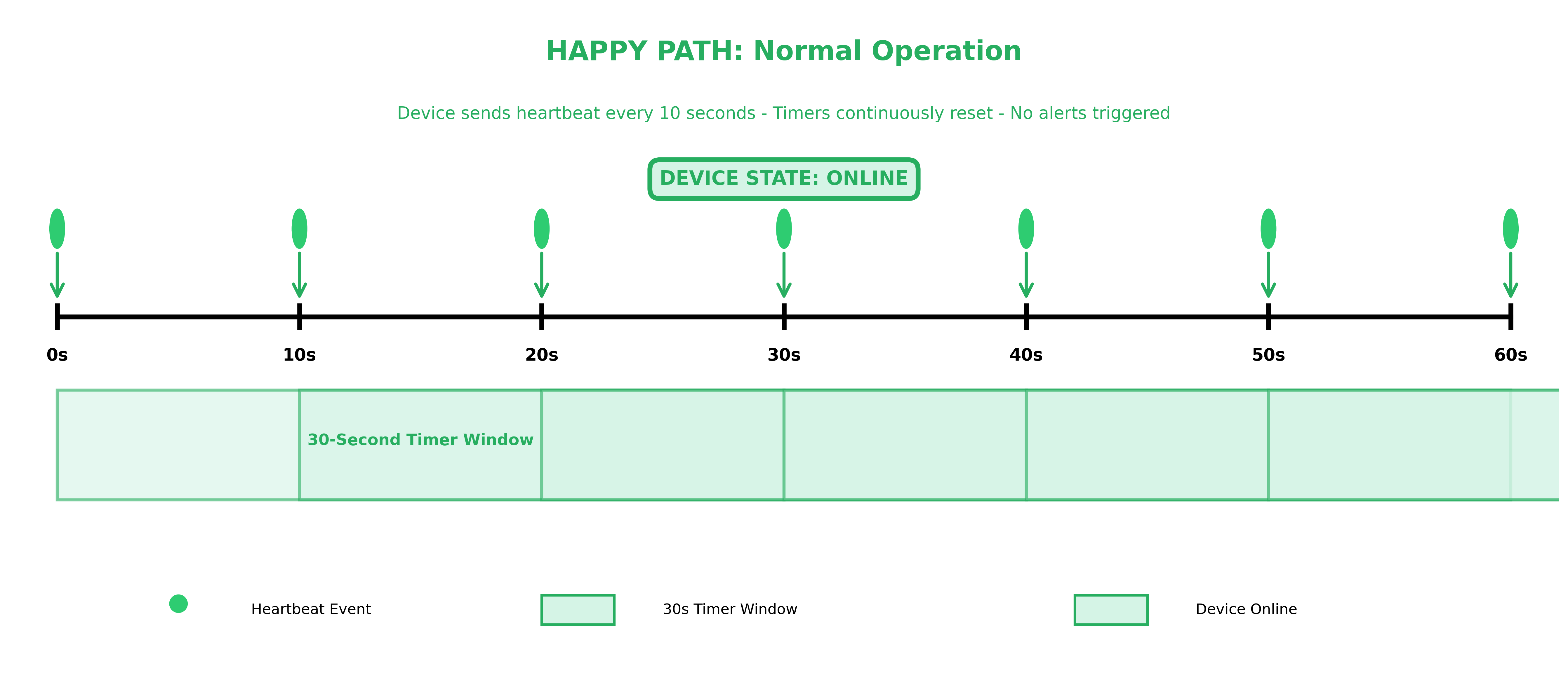
Timeline diagram showing normal device operation over 60 seconds with heartbeats arriving every 10 seconds, each resetting the 30-second timer

The above timeline diagram shows a 60-second window of normal device operation. Heartbeat events arrive every 10 seconds (at 0s, 10s, 20s, 30s, 40s, 50s, and 60s), each resetting the 30-second timer window. Because every heartbeat arrives well within the 30-second threshold, the timer never expires, the device state remains online, and no alerts are triggered.

Step 4: Test offline detection

Stop sending heartbeat events for the device and wait 30 seconds. You should receive an SNS alert indicating the device is offline.
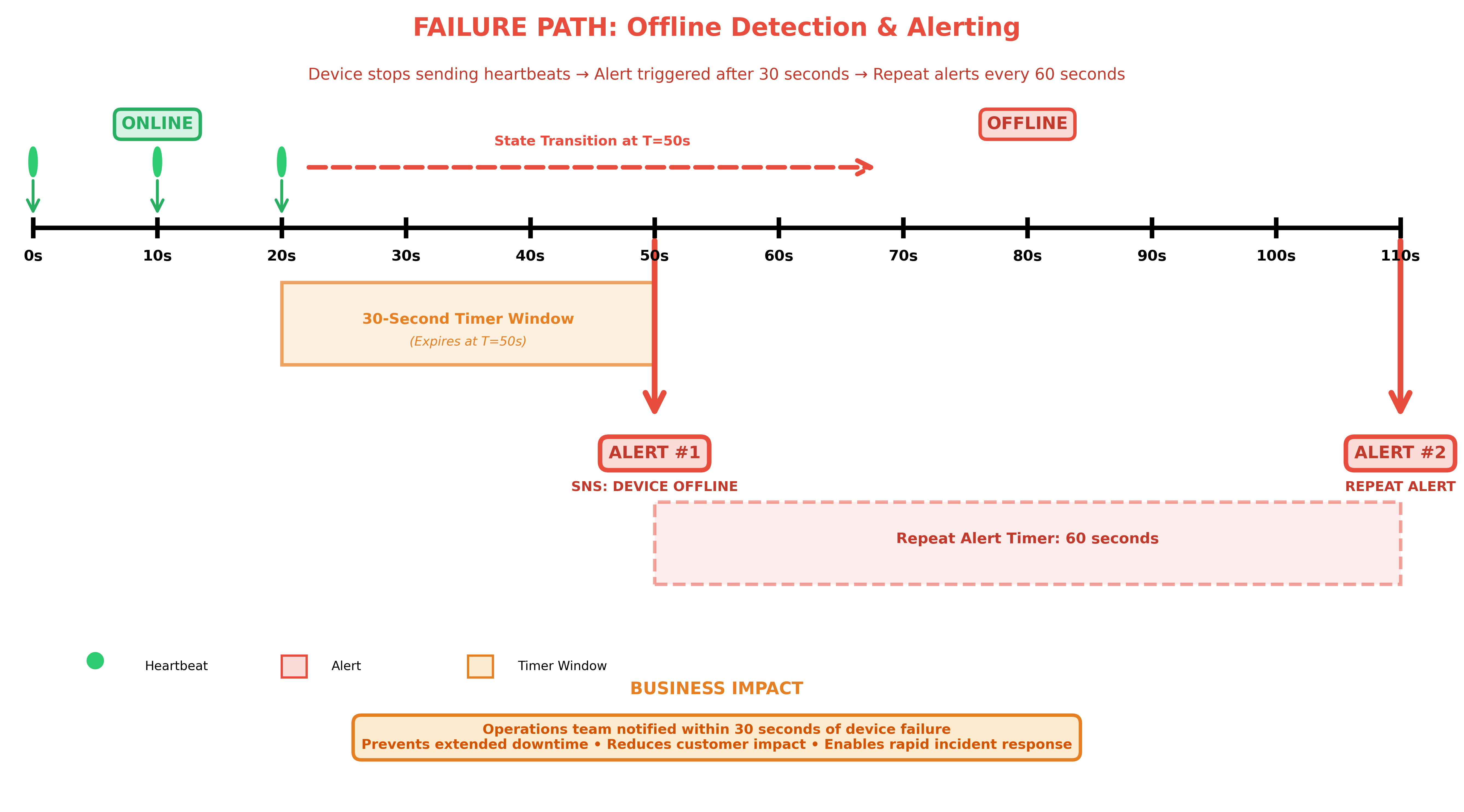
Timeline diagram showing offline detection over 110 seconds with the 30-second timer expiring and triggering SNS alerts

Timeline diagram showing offline detection over 110 seconds. Device sends heartbeats at 0s, 10s, and 20s before going offline. The 30-second timer expires at 50s triggering Alert #1 via SNS, followed by a repeat Alert #2 at 110s after a 60-second repeat timer.

If you continue to not send heartbeats, additional alerts will be sent every 60 seconds.

Step 5: Test device recovery

Resume sending heartbeat events using the same CLI command. The application will cancel all existing timers for the device and will stop sending SNS alerts.
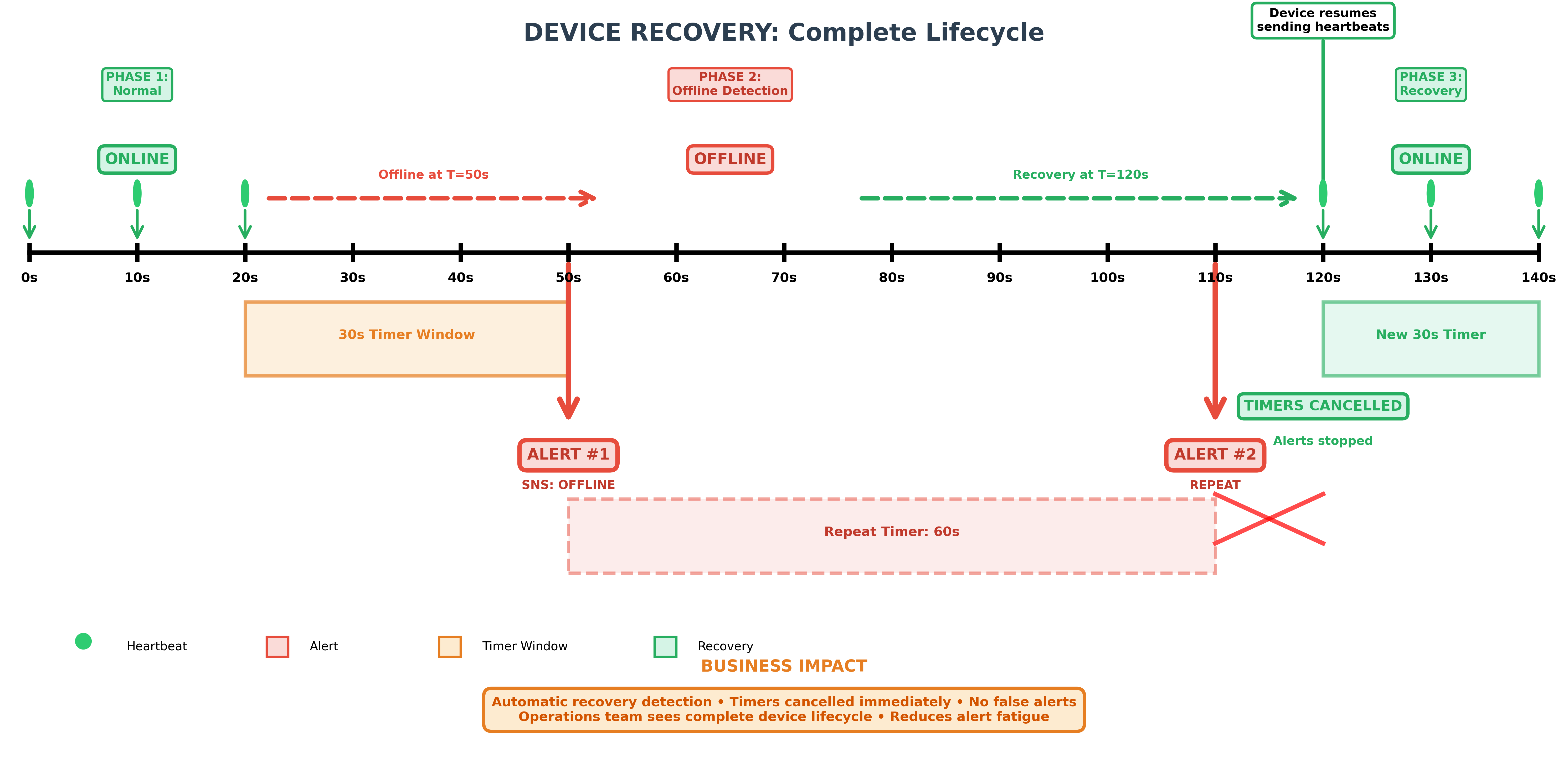
Timeline diagram showing device recovery lifecycle with timers canceled and device returning to online state

Timeline diagram showing the complete device recovery lifecycle over 140 seconds across three phases: normal operation with heartbeats, offline detection with SNS alerts, and recovery where timers are canceled and the device returns to online state

Clean up

To avoid incurring ongoing charges, follow these steps to clean up the resources.

Step 1: Stop the EMR serverless application

Stop your running streaming job:

aws emr-serverless stop-job-run \
  --application-id <your-application-id> \
  --job-run-id <your-job-run-id>

Step 2: Delete the EMR serverless application

aws emr-serverless delete-application \
  --application-id <your-application-id>

Step 3: Delete kinesis data stream

aws kinesis delete-stream --stream-name iot-heartbeat

Step 4: Remove S3 objects

Delete the checkpoint data, scripts, and dependencies from your S3 bucket:

aws s3 rm s3://your-bucket/checkpoints/ --recursive
aws s3 rm s3://your-bucket/scripts/ --recursive
aws s3 rm s3://your-bucket/jars/ --recursive
aws s3 rm s3://your-bucket/pyfiles/ --recursive

Real-world use cases for stateful streaming

The transformWithState API enables developers to build sophisticated streaming applications that were previously difficult to implement. Here are a few examples of how it can be applied across industries.

Telecommunications and network monitoring: Telecom providers need to detect network anomalies and SLA violations as they happen across millions of concurrent sessions. With transformWithState, developers can maintain per-session state to track call detail records, compare real-time network metrics against established baselines, and trigger alerts the moment thresholds are breached. Automatic state TTL ensures that completed session records are cleaned up without manual intervention.

Financial services and fraud detection: Detecting fraud requires correlating multiple signals across a sequence of transactions in real time. With transformWithState, developers can maintain per-account state that tracks transaction histories, flags suspicious patterns like rapid purchases across geographies, and calculates rolling risk scores. Multiple state variables per key allow tracking different dimensions of activity, such as transaction velocity, location changes, and spending deviations, within a single stateful operator.

E-commerce and customer engagement: Understanding customer behavior in real time is critical for driving conversions. Using transformWithState, developers can build session-aware applications that track browsing and cart activity with timer-based state expiration, detecting cart abandonment after a configurable timeout and triggering personalized re-engagement notifications. The State Data Source Reader enables teams to inspect session state mid-stream, making it easier to debug and validate real-time customer journey logic.

Conclusion

Apache Spark 4.0’s transformWithState API represents a significant advancement in stateful stream processing, making it simpler to build complex real-time applications like IoT device monitoring. Combined with Amazon EMR Serverless, you get a fully managed platform that scales automatically and eliminates infrastructure management overhead.

This post demonstrates how to use the native timer support capability of transformWithState to build a real-time IoT device monitoring application. We encourage you to explore other capabilities such as Automatic State TTL, Schema Evolution, and Multiple State Variables on Amazon EMR Serverless to build more sophisticated streaming applications tailored to your needs.

About the authors

Raj Ramasubbu

Raj Ramasubbu

Raj Ramasubbu is a Senior Specialist Solutions Architect for Analytics and AI at AWS. He partners with ISV customers to design and implement modern data platforms that balance performance, cost efficiency, and operational resilience at scale. With over two decades of experience spanning data engineering, advanced analytics, and machine learning across industries such as healthcare, financial services, and retail, Raj brings a practitioner’s perspective to solving complex data challenges in the cloud.

Rekha Veeraraghavan

Rekha Veeraraghavan

Rekha Veeraraghavan is a Technical Account Manager at Amazon Web Services (AWS). She serves as a Subject Matter Expert in AWS Analytics services, specializing in AWS Glue and Amazon Athena. Rekha provides expert guidance and technical support to enterprise and strategic customers, helping them optimize data analytics solutions. With deep expertise in data engineering, she enables organizations to build scalable, efficient, and cost-effective data processing pipelines on AWS.

Praveen Krishnamoorthy Ravikumar

Praveen Krishnamoorthy Ravikumar

Praveen Krishnamoorthy Ravikumar is an Analytics Specialist Solutions Architect at AWS. He helps customers design and implement modern data and analytics platforms that leverage the scalability, flexibility, and innovation of the cloud. He is passionate about solving complex data challenges and enabling organizations to unlock actionable insights from their data.

Deploy real-time analytics with StarTree for managed Apache Pinot on AWS

Post Syndicated from Raj Ramasubbu original https://aws.amazon.com/blogs/big-data/deploy-real-time-analytics-with-startree-for-managed-apache-pinot-on-aws/

This post is cowritten with Mayank Shrivastava and Barkha Herman from StarTree.

Building a low-latency, high-concurrency, real-time online analytical processing (OLAP) solution has been previously explored on the AWS Big Data Blog, where we walked through how to build a real-time analytics solution with Apache Pinot on AWS, in which streaming sources, such as Amazon Managed Streaming for Apache Kafka (Amazon MSK) and Amazon Kinesis Data Streams, produce events that are ingested and processed in real time within Apache Pinot.

However, this approach requires self-management of the infrastructure required to run Pinot, as well as a number of manual processes to run in production. StarTree is a managed alternative that offers similar benefits for real-time analytics use cases.

In this post, we introduce StarTree as a managed solution on AWS for teams seeking the advantages of Pinot. We highlight the key distinctions between open-source Pinot and StarTree, and provide valuable insights for organizations considering a more streamlined approach to their real-time analytics infrastructure.

By examining these aspects, you can make an informed decision between open source Pinot and StarTree for your specific real-time analytics needs.

StarTree overview

One of the founders of Apache Pinot, Kishore Gopalakrishna, launched StarTree to equip organizations globally with the power of real-time data and build a fully managed platform for real-time analytics. Handling over 1 billion queries per week and ingesting over 1 million events per second, StarTree Cloud removes the burden of infrastructure management so companies can focus on delivering real-time insights to end-users.

Open source Pinot requires in-house expertise that can challenge well-established technical teams to provision hardware, configure environments, tune performance, maintain security, adhere to data governance requirements, manage software updates, and constantly monitor for system issues. Organizations interested in decreasing their time to value with a managed Pinot solution can take advantage of the expertise of StarTree’s team to accelerate setup, deploy an architecture ready for scale, and offload infrastructure maintenance.

Improving security with SOC 2, SSO, and RBAC

Critical enterprise security features can be challenging to implement in open source Pinot environments. With StarTree’s managed Pinot, role-based access control (RBAC) simplifies administration for Pinot and allows organizations to assign and monitor user access based on roles to enforce secure and efficient access to sensitive data. StarTree Cloud provides enterprise-grade security with SOC 2 compliance, enhanced encryption, and single sign-on (SSO) capabilities.

Using automated data ingestion at scale

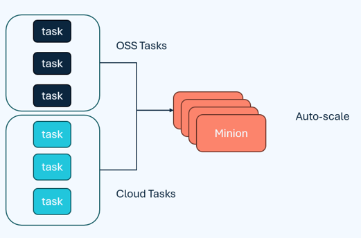
The minion task framework is a native component of Pinot to offload computationally intensive tasks away from the other Pinot components to conserve resources for low-latency queries and support real-time stream ingestion. StarTree can handle larger volumes of data efficiently with highly scalable implementations of minion tasks and a minion auto scaling feature that eliminates unnecessary infrastructure costs during idle times, as seen in the below figure.

StarTree’s automatic data ingestion framework is ideal for enterprise workloads because it improves scalability and reduces the data maintenance complexity often found in open source Pinot deployments. StarTree supports a large number of managed connectors, which are used to maintain metadata about the source and ingest data seamlessly into the platform. The data is then modelled to help you organize and structure the data fetched from the selected data source into Pinot tables. Indexes are then configured to optimize query performance, as per the flow in the diagram below.

Tiered storage for real-time query processing

With open source Pinot, tiered storage can be used for deep storage like Amazon Simple Storage Service (Amazon S3) for backup but not query processing, because storage is tightly coupled with compute and requires manual configuration of tenants with different storage speeds and server specifications. In the following diagram, an Amazon S3 tier is defined for the data to be moved from tightly coupled SSD to cloud storage when the data is 30 days old.


On the other hand, StarTree transitions less-frequently accessed data to cost-effective storage like Amazon S3, while maintaining quick access to frequently accessed data. StarTree’s tiered storage enables automation for real-time query processing with index pinning, prefetching, and intelligent data movement between hot and cold storage, optimizing both performance and cost. StarTree’s sophisticated approach to tiered storage is highly flexible and reduces replication overhead by keeping a single copy in cloud storage, which prevents the limitations of compressed deep store copies, as you can see in the below diagram

Improving scalability with off-heap upserts

Companies like Amberdata benefit from StarTree’s upsert support to routinely upsert 350,000 events per second, with peak workloads reaching 1 million upserts per second. StarTree Cloud enhanced upsert functionality boosts efficiency, usability, and scalability through the implementation of off-heap upserts. Behind the scenes, Pinot servers manage specific upsert metadata to determine if a newly inserted record’s primary key was previously encountered and identifies the current segment holding it. As shown below, StarTree Cloud moves this off-heap, enabling a scalable cache of metadata as the on-heap memory restrictions are removed

Customer success stories using Pinot with StarTree for real-time analytics

The following customers highlight their success using Pinot for StarTree:

Flexible deployment options for StarTree Cloud

StarTree offers multiple deployment options, including a StarTree hosted software as a service (SaaS) or customer hosted SaaS. StarTree hosted SaaS is ideal for organizations interested in fully offloading the operational burden of infrastructure management, scaling, performance tuning, and security from their team so they can focus on analytics. StarTree’s customer hosted SaaS provides flexibility for customers interested in deploying the solution within their AWS environment or other platform of choice. This is suitable for organizations who require higher infrastructure management controls in their perimeter but still want the operational ease of a managed service.

Self-managed Pinot or StarTree

Pinot can deliver value for real-time analytics scenarios with different deployment methods. The choice of deployment method will come down to organizational priorities and trade-offs. Teams with the capability and willingness to manage open source software on a commodity infrastructure at scale might opt to deploy self-managed Pinot on AWS. Teams interested in reducing time troubleshooting performance bottlenecks, optimizing resource usage, and minimizing downtime can use StarTree’s managed service.

Conclusion

In this post, we presented StarTree as a managed solution on AWS for teams seeking the advantages of Apache Pinot. Like Pinot, StarTree addresses the need for a low-latency, high-concurrency, real-time online analytical processing (OLAP) solution. In addition, StarTree offers a managed experience for real-time and batch Pinot workloads, offering enhanced security, automated data ingestion, tiered storage, and off-heap upserts. These features improve security, scalability, and manageablity for organizations looking to run Pinot in production.

Developers interested in learning more about managed Pinot can deploy real-time analytics with StarTree to test it out or join a session with StarTree’s head of product. StarTree is an AWS ISVA partner and is available on AWS Marketplace.


About the Authors

Raj Ramasubbu is a Senior Analytics Specialist Solutions Architect focused on big data and analytics and AI/ML with Amazon Web Services. He helps customers architect and build highly scalable, performant, and secure cloud-based solutions on AWS. Raj provided technical expertise and leadership in building data engineering, big data analytics, business intelligence, and data science solutions for over 18 years prior to joining AWS. He helped customers in various industry verticals like healthcare, medical devices, life science, retail, asset management, car insurance, residential REIT, agriculture, title insurance, supply chain, document management, and real estate.

Francisco Morillo is a Streaming Solutions Architect at AWS. Francisco works with AWS customers, helping them design real-time analytics architectures using AWS services, supporting Amazon Managed Streaming for Apache Kafka (Amazon MSK) and Amazon Managed Service for Apache Flink.

Ismail Makhlouf is a Senior Specialist Solutions Architect for Data Analytics at AWS. Ismail focuses on architecting solutions for organizations across their end-to-end data analytics estate, including batch and real-time streaming, big data, data warehousing, and data lake workloads. He primarily partners with airlines, manufacturers, and retail organizations to support them to achieve their business objectives with well-architected data platforms.

Renee Berry is a Senior Partner Development Manager with the AWS Global Startup Program, working with venture backed startups partnering with AWS to scale their growth.

Mayank Shrivastava is a founding engineer of Apache Pinot and a PMC member for the project. He is currently a Fellow at StarTree Inc., where he also heads their Center of Excellence.

Barkha Herman is a technologist and developer advocate who founded WiTVoices and South Florida Women in Tech. She fosters inclusive tech communities.

Read and write S3 Iceberg table using AWS Glue Iceberg Rest Catalog from Open Source Apache Spark

Post Syndicated from Raj Ramasubbu original https://aws.amazon.com/blogs/big-data/read-and-write-s3-iceberg-table-using-aws-glue-iceberg-rest-catalog-from-open-source-apache-spark/

In today’s data-driven world, organizations are constantly seeking efficient ways to process and analyze vast amounts of information across data lakes and warehouses.

Enter Amazon SageMaker Lakehouse, which you can use to unify all your data across Amazon Simple Storage Service (Amazon S3) data lakes and Amazon Redshift data warehouses, helping you build powerful analytics and AI and machine learning (AI/ML) applications on a single copy of data. SageMaker Lakehouse gives you the flexibility to access and query your data in-place with all Apache Iceberg compatible tools and engines. This opens up exciting possibilities for Open Source Apache Spark users who want to use SageMaker Lakehouse capabilities. Further you can secure your data in SageMaker Lakehouse by defining fine-grained permissions, which are enforced across all analytics and ML tools and engines.

In this post, we will explore how to harness the power of Open source Apache Spark and configure a third-party engine to work with AWS Glue Iceberg REST Catalog. The post will include details on how to perform read/write data operations against Amazon S3 tables with AWS Lake Formation managing metadata and underlying data access using temporary credential vending.

Solution overview

In this post, the customer uses Data Catalog to centrally manage technical metadata for structured and semi-structured datasets in their organization and wants to enable their data team to use Apache Spark for data processing. The customer will create an AWS Glue database and configure Apache Spark to interact with Glue Data Catalog using the Iceberg Rest API for writing/reading Iceberg data on Amazon S3 using Lake Formation permission control.

We will start by running an extract, transform, and load (ETL) script using Apache Spark to create an Iceberg table on Amazon S3 and access the table using the Glue Iceberg REST Catalog. The ETL script will add data to the Iceberg table and then read it back using Spark SQL. This post will showcase how this data can also be queried by other data teams using Amazon Athena .

Prerequisites

Access to an AWS Identity and Access Management (IAM) role that is a Lake Formation data lake administrator in the account that has the Data Catalog. For instructions, see Create a data lake administrator.

  1. Verify that you have Python version 3.7 or later installed. Check if pip3 version is 22.2.2 or higher is installed.
  2. Install or update the latest AWS Command Line Interface (AWS CLI). For instructions, see Installing or updating the latest version of the AWS CLI. Run aws configure using AWS CLI to point to your AWS account.
  3. Create an S3 bucket to store the customer Iceberg table. For this post, we will be using the us-east-2 AWS Region and will name the bucket: ossblog-customer-datalake.
  4. Create an IAM role that will be used in OSS Spark for data access using an AWS Glue Iceberg REST catalog endpoint. Make sure that the role has AWS Glue and Lake Formation policies as defined in Data engineer permissions. For this post, we will use an IAM role named spark_role.

Enable Lake Formation permissions for third-party access

In this section, you will register the S3 bucket with Lake Formation. This step allows Lake Formation to act as a centralized permissions management system for metadata and data stored in Amazon S3, enabling more efficient and secure data governance in data lake environments.

  1. Create a user defined IAM role following the instructions in Requirements for roles used to register locations. For this post, we will use the IAM role: LFRegisterRole.
  2. Register the S3 bucket ossblog-customer-datalake using the IAM role LFRegisterRole by running the following command:
    aws lakeformation register-resource \
    --resource-arn '< S3 bucket ARN for amzn-s3-demo-bucket>' \
    --role-arn '< IAM Role ARN for LFRegisterRole >' \
    --region <aws_region>

Alternatively you can use the AWS Management Console for Lake Formation.

  1. Navigate to the Lake Formation console, choose Administration in the navigation pane, and then Data lake locations and provide the following values:
    1. For Amazon S3 path, select s3://ossblog-customer-datalake.
    2. For IAM role, select LFRegisterRole
    3. For Permission mode, choose Lake Formation.
    4. Choose Register location.
  1. In Lake Formation, enable full table access for external engines to access data.
    1. Sign in as an admin user, choose Administration in the navigation pane.
    2. Choose Application integration settings and select Allow external engines to access data in Amazon S3 locations with full table access.
    3. Choose Save.

Set up resource access for the OSS Spark role:

  1. Create an AWS Glue database called ossblogdb in the default catalog by going to the Lake Formation console and choosing Databases in the navigation pane.
  2. Select the database, choose Edit and clear the checkbox for Use only IAM access control for new tables in this database.

Grant resource permission to OSS  Spark role:

To enable OSS Spark to create and populate the dataset in the ossblogdb database, you will use the IAM role (spark_role) for Apache Spark instance that you created in step 4 of the prerequisites section. Apache Spark will assume this role to create an Iceberg table, add records to it and read from it. To enable this functionality, grant full table access to spark_role and provide data location permission to the S3 bucket where the table data can be stored.

Grant create table permission to the spark_role:

Sign in as Datalake Admin and run the following command using AWS CLI:

aws lakeformation grant-permissions \
--principal '{"DataLakePrincipalIdentifier":"arn:aws:iam::<aws_account_id>:role/<iam_role_name>"}' \
--permissions '["CREATE_TABLE","DESCRIBE"]'\
--resource '{"Database":{"CatalogId":"<aws_account_id>","Name":"ossblogdb"}}' \
--region <aws_region>

Alternatively on the console:

  1. In the Lake Formation console navigation pane, choose Data lake permissions, and then choose Grant.
  2. In the Principals section, for IAM users and roles, select spark_role.
  3. In the LF-Tags or catalog resources section, select Named Data Catalog resources:
    1. Select <accountid> for Catalogs.
    2. Select ossblogdb for Databases.
  4. Select DESCRIBE and CREATE TABLE for Database permissions.
  5. Choose Grant.

Grant data location permission to the spark_role:

Sign in as Datalake Admin and run the following command using the AWS CLI:

aws lakeformation grant-permissions 
--principal '{"DataLakePrincipalIdentifier":"<Principal>"}' 
--permissions DATA_LOCATION_ACCESS 
--resource '{"DataLocation":{"CatalogId":"<Catalog ID>","ResourceArn":"<S3 bucket ARN>"}}' 
--region <aws_region>

Alternatively on the console:

  1. In the Lake Formation console navigation pane, choose Data Locations, and then choose Grant.
  2. For IAM users and roles, select spark_role.
  3. For Storage locations, select the bucket_name
  4. Choose Grant.

Set up a Spark script to use an AWS Glue Iceberg REST catalog endpoint:

Create a file named oss_spark_customer_etl.py in your environment with the following content:

import sys
import os
import time
from pyspark.sql import SparkSession

#Replace <aws_region> with AWS region name.
#Replace <aws_account_id> with AWS account ID.

spark = SparkSession.builder.appName('osspark') \
.config('spark.jars.packages', 'org.apache.iceberg:iceberg-spark-runtime-3.5_2.12:1.4.1,software.amazon.awssdk:bundle:2.20.160,software.amazon.awssdk:url-connection-client:2.20.160') \
.config('spark.sql.extensions', 'org.apache.iceberg.spark.extensions.IcebergSparkSessionExtensions') \
.config('spark.sql.defaultCatalog', 'spark_catalog') \
.config('spark.sql.catalog.spark_catalog', 'org.apache.iceberg.spark.SparkCatalog') \
.config('spark.sql.catalog.spark_catalog.type', 'rest') \
.config('spark.sql.catalog.spark_catalog.uri','https://glue.<aws_region>.amazonaws.com/iceberg') \
.config('spark.sql.catalog.spark_catalog.warehouse','<aws_account_id>') \
.config('spark.sql.catalog.spark_catalog.rest.sigv4-enabled','true') \
.config('spark.sql.catalog.spark_catalog.rest.signing-name','glue') \
.config('spark.sql.catalog.spark_catalog.rest.signing-region', <aws_region>) \
.config('spark.sql.catalog.spark_catalog.io-impl','org.apache.iceberg.aws.s3.S3FileIO') \
.config('spark.hadoop.fs.s3a.aws.credentials.provider','org.apache.hadoop.fs.s3a.SimpleAWSCredentialProvider') \
.config('spark.sql.catalog.spark_catalog.rest-metrics-reporting-enabled','false') \
.getOrCreate()
spark.sql("use ossblogdb").show()
spark.sql("""CREATE TABLE ossblogdb.customer (name string) USING iceberg location 's3://<3_bucket_name>/customer'""")
time.sleep(120)
spark.sql("insert into ossblogdb.customer values('Alice') ").show()
spark.sql("select * from ossblogdb.customer").show()

Launch Pyspark locally and validate read/write to the Iceberg table on Amazon S3

Run pip install pyspark. Save the script locally and set the environment variables (AWS_ACCESS_KEY_ID, AWS_SECRET_ACCESS_KEY, and AWS_SESSION_TOKEN) with temporary credentials for the spark_role IAM role.

Run python /path/to/oss_spark_customer_etl.py

You can also use Athena to view the data in the Iceberg table:

To enable the other data team to view the content, provide read access to the data team IAM role using the Lake Formation console:

  1. In the Lake Formation console navigation pane, choose Data lake permissions, and then choose Grant.
  2. In the Principals section, for IAM users and roles choose <iam_role>.
  3. In the LF-Tags or catalog resources section, select Named Data Catalog resources:
    1. Select <accountid> for Catalogs.
    2. Select ossblogdb for Databases.
    3. Select customer for Tables.
  4. Select DESCRIBE and SELECT for Table permissions.
  5. Choose Grant.

Sign in as the IAM role and run the command:

SELECT * FROM "ossblogdb"."customer" limit 10;

Clean up

To clean up your resources, complete the following steps:

  1. Delete the resources database/table created in Data Catalog.
  2. Empty and then delete the S3 bucket

Conclusion

In this post, we’ve walked through the seamless integration between Apache Spark and an AWS Glue Iceberg Rest Catalog for accessing Iceberg tables in Amazon S3, demonstrating how to effectively perform read and write operations using Iceberg REST API. The beauty of this solution lies in its flexibility—whether you’re running Spark on bare metal servers in your data center, in a Kubernetes cluster, or any other environment, this architecture can be adapted to suit your needs.


About the Authors

Raj RamasubbuRaj Ramasubbu is a Sr. Analytics Specialist Solutions Architect focused on big data and analytics and AI/ML with Amazon Web Services. He helps customers architect and build highly scalable, performant, and secure cloud-based solutions on AWS. Raj provided technical expertise and leadership in building data engineering, big data analytics, business intelligence, and data science solutions for over 20 years prior to joining AWS. He helped customers in various industry verticals like healthcare, medical devices, life science, retail, asset management, car insurance, residential REIT, agriculture, title insurance, supply chain, document management, and real estate.

Srividya Parthasarathy is a Senior Big Data Architect on the AWS Lake Formation team. She works with product team and customer to build robust features and solutions for their analytical data platform.  She enjoys building data mesh solutions and sharing them with the community.

Pratik Das is a Senior Product Manager with AWS Lake Formation. He is passionate about all things data and works with customers to understand their requirements and build delightful experiences. He has a background in building data-driven solutions and machine learning systems in production.

Build a real-time analytics solution with Apache Pinot on AWS

Post Syndicated from Raj Ramasubbu original https://aws.amazon.com/blogs/big-data/build-a-real-time-analytics-solution-with-apache-pinot-on-aws/

Online Analytical Processing (OLAP) is crucial in modern data-driven apps, acting as an abstraction layer connecting raw data to users for efficient analysis. It organizes data into user-friendly structures, aligning with shared business definitions, ensuring users can analyze data with ease despite changes. OLAP combines data from various data sources and aggregates and groups them as business terms and KPIs. In essence, it’s the foundation for user-centric data analysis in modern apps, because it’s the layer that translates technical assets into business-friendly terms that enable users to extract actionable insights from data.

Real-time OLAP

Traditionally, OLAP datastores were designed for batch processing to serve internal business reports. The scope of data analytics has grown, and more user personas are now seeking to extract insights themselves. These users often prefer to have direct access to the data and the ability to analyze it independently, without relying solely on scheduled updates or reports provided at fixed intervals. This has led to the emergence of real-time OLAP solutions, which are particularly relevant in the following use cases:

  • User-facing analytics – Incorporating analytics into products or applications that consumers use to gain insights, sometimes referred to as data products.
  • Business metrics – Providing KPIs, scorecards, and business-relevant benchmarks.
  • Anomaly detection – Identifying outliers or unusual behavior patterns.
  • Internal dashboards – Providing analytics that are relevant to stakeholders across the organization for internal use.
  • Queries – Offering subsets of data to users based on their roles and security levels, allowing them to manipulate data according to their specific requirements.

Overview of Apache Pinot

Building these capabilities in real time means that real-time OLAP solutions have stricter SLAs and larger scalability requirements than traditional OLAP datastores. Accordingly, a purpose-built solution is needed to address these new requirements.

Apache Pinot is an open source real-time distributed OLAP datastore designed to meet these requirements, including low latency (tens of milliseconds), high concurrency (hundreds of thousands of queries per second), near real-time data freshness, and handling petabyte-scale data volumes. It ingests data from both streaming and batch sources and organizes it into logical tables distributed across multiple nodes in a Pinot cluster, ensuring scalability.

Pinot provides functionality similar to other modern big data frameworks, supporting SQL queries, upserts, complex joins, and various indexing options.

Pinot has been tested at very large scale in large enterprises, serving over 70 LinkedIn data products, handling over 120,000 Queries Per Second (QPS), ingesting over 1.5 million events per second, and analyzing over 10,000 business metrics across over 50,000 dimensions. A notable use case is the user-facing Uber Eats Restaurant Manager dashboard, serving over 500,000 users with instant insights into restaurant performance.

Pinot clusters are designed for high availability, horizontal scalability, and live configuration changes without impacting performance. To that end, Pinot is architected as a distributed datastore to enable all of the above requirements, and utilizes similar architectural constructs as Apache Kafka and Apache Hadoop in its design.

Solution overview

In this, we will provide a step-by-step guide showing you how you can build a real-time OLAP datastore on Amazon Web Services (AWS) using Apache Pinot on Amazon Elastic Compute Cloud (Amazon EC2) and do near real-time visualization using Tableau. You can use Apache Pinot for batch processing use cases as well but, in this post, we will focus on a near real-time analytics use case.

You can use Amazon Managed Service for Apache Flink service. The objective in the preceding figure is to ingest streaming data into Pinot, where it can perform.

Blog post architecture

The objective in the preceding figure is to ingest streaming data into Pinot, where it can perform aggregations, update current data models, and serve OLAP queries in real time to consuming users and applications, which in this case is a user-facing Tableau dashboard.

The data flow as follows:

  • Data is ingested from a real-time source, such as clickstream data from a website. For the purposes of this post, we will use the Amazon Kinesis Data Generator to simulate the production of events.
  • Events are captured in a streaming storage platform such as or Amazon Managed Streaming for Apache Kafka (MSK) for downstream consumption.
  • The events are then ingested into the real-time server within Apache Pinot, which is used to process data coming from streaming sources, such as MSK and KDS. Apache Pinot consists of logical tables, which are partitioned into segments. Due to the time sensitive nature of streaming, events are directly written into memory as consuming segments, which can be thought of as parts of an active table that are continuously ingesting new data. Consuming segments are available for query processing immediately, thereby enabling low latency and high data freshness.
  • After the segments reach a threshold in terms of time or number of rows, they are moved into Amazon Simple Storage Service (Amazon S3), which serves as deep storage for the Apache Pinot cluster. Deep storage is the permanent location for segment files. Segments used for batch processing are also stored there.
  • In parallel, the Pinot controller tracks the metadata of the cluster and performs actions required to keep the cluster in an ideal state. Its primary function is to orchestrate cluster resources as well as manage connections between resources within the cluster and data sources outside of it. Under the hood, the controller uses Apache Helix to manage cluster state, failover, distribution, and scalability and Apache Zookeeper to handles distributed coordination functions such as leader election, locks, queue management, and state tracking.
  • To enable the distributed aspect of the Pinot architecture, the broker accepts queries from the clients and forwards them to servers and collects the results and sends them back. The broker manages and optimizes the queries, distributes them across the servers, combines the results, and returns the result set. The broker sends the request to the right segments on the right servers, optimizes segment pruning, and splits the queries across servers appropriately. The results of each query are then merged and sent back to the requesting client.
  • The results of the queries are updated in real time in the Tableau dashboard.

To ensure high availability, the solution deploys application load balancers for the brokers and servers. We can access the Apache Pinot UI using the controller load balancer and use it to run queries and monitor the Apache Pinot cluster

Let’s start to deploy this solution and perform near real-time visualizations using Apache Pinot and Tableau.

Prerequisites

Before you get started, make sure you have the following prerequisites:

Deploy the Apache Pinot solution using the AWS CDK

The AWS CDK is an open source project that you can use to define your cloud infrastructure using familiar programming languages. It uses high-level constructs to represent AWS components to simplify the build process. In this post, we use TypeScript and Python to define the cloud infrastructure.

  1. First, bootstrap the AWS CDK. This sets up the resources required by the AWS CDK to deploy into the AWS account. This step is only required if you haven’t used the AWS CDK in the deployment account and Region. The format for the bootstrap command is cdk bootstrap aws://<account-id>/<aws-region>.

In the following example, I’m running a bootstrap command for a fictitious AWS account with ID 123456789000 and us-east-1 N.Virginia Region:

cdk bootstrap aws://123456789000/us-east-1

Bootstrap command

  1. Next, clone the GitHub repository and install all the dependencies from package.json by running the following commands from the root of the cloned repository.
    git clonehttps://github.com/aws-samples/near-realtime-apache-pinot-workshop
    
    cd near-realtime-apache-pinot-workshop
    
    npm i

  2. Deploy the AWS CDK stack to create the AWS Cloud infrastructure by running the following command and enter y when prompted. Enter the IP address that you want to use to access the Apache Pinot controller and broker in /32 subnet mask format.
    cdk deploy --parameters IpAddress="<YOUR-IP-ADDRESS-IN-/32-SUBNET-MASK-FORMAT>"

Deployment of the AWS CDK stack takes approximately 10–12 minutes. You should see a stack deployment message that will display the creation of AWS objects, followed by the deployment time, the Stack ARN, and the total time, similar to the following screenshot:

CDK deployment screenshot

  1. Now, you can get the Apache Pinot controller Application Load Balancer (ALB) DNS name from the Copy the value for ControllerDNSUrl.
  2. Launch a browser session and paste the DNS name to see the Apache Pinot controller—it should look like the following screenshot, where you will see:
    • Number of controllers, brokers, servers, minions, tenants, and tables
    • List of tenants
    • List of controllers
    • List of brokers

Pinot management console

Near real-time visualization using Tableau

Now that we have provisioned all AWS Cloud resources, we will stream some sample web transactions to a Kinesis data stream and visualize the data in near real time from Tableau Desktop.

You can follow these steps to open the Tableau workbook to visualize

  1. Download the Tableau workbook to your local machine and open the workbook from Tableau Desktop.
  2. Get the DNS name for Apache Pinot broker’s Application Load Balancer DNS name from the CloudFormation console. Choose Stacks, select the ApachePinotSolutionStack, and then choose Outputs and copy the value for BrokerDNSUrl.
  3. Choose Edit connection and enter the URL in the following format:
    jdbc:pinot://<Apache-Pinot-Controller-DNS-Name>?brokers=<Apache-Pinot-Broker-DNS-Name>

  4. Enter admin for both the username and password.
  5. Access the KDG tool by following the instructions. Use the record template that follows to send sample web transactions data to Kinesis Data streams called pinot-stream by choosing Send dataas shown in the following screenshot. Stop sending data after sending a handful of records by choosing Stop sending data to Kinesis.
{
"userID" : "{{random.number(
{
"min":1,
"max":100
}
)}}",
"productName" : "{{commerce.productName}}",
"color" : "{{commerce.color}}",
"department" : "{{commerce.department}}",
"product" : "{{commerce.product}}",
"campaign" : "{{random.arrayElement(
["BlackFriday","10Percent","NONE"]
)}}",
"price" : {{random.number(
{   "min":10,
"max":150
}
)}},
"creationTimestamp" : "{{date.now("YYYY-MM-DD hh:mm:ss")}}"
}

Kinesis Data Generator configuration

You should be able to see the web transactions data in Tableau Desktop as shown in the following screenshot.

Clean up

To clean up the AWS resources you created:

  1. Disable termination protection on the following EC2 instances by going to the Amazon EC2 console and choosing Instance from the navigation pane. Choose Actions, Instance Settings, and then Change termination protection and clear the Termination protection checkbox.
    • ApachePinotSolutionStack/bastionHost
    • ApachePinotSolutionStack/zookeeperNode1
    • ApachePinotSolutionStack/zookeeperNode2
    • ApachePinotSolutionStack/zookeeperNode3
  2. Run the following command from the cloned GitHub repo and enter y when prompted.
    cdk destroy

Scaling the solution to production

The example in this post uses minimal resources to demonstrate functionality. Taking this to production requires a higher level of scalability. The solution provides autoscaling policies for independently scaling brokers and servers in and out, allowing the Apache Pinot custer to scale based on CPU requirements.

When autoscaling is initiated, the solution will invoke an AWS Lambda Function, to run the logic needed to add or remove brokers and servers in Apache Pinot.

In Apache Pinot, tables are tagged with an identifier that’s used for routing queries to the appropriate servers. When creating a table, you can specify a table name and optionally tag it. This is useful when you want to route queries to specific servers or build a multi-tenant Apache Pinot cluster. However, tagging adds additional considerations when removing brokers or servers. You need to make sure that neither have any active tables or tags associated with them. And when adding new components, rebalance the segments, so you can use the new brokers and servers.

Therefore, when scaling is needed in the solution, the autoscaling policy will invoke a Lambda function that either rebalances the segments of the tables when you add a new broker or server, or removes any tags associated with the broker or server you remove from the cluster.

Summary

Just like you would commonly use a distributed NoSQL datastore to serve a mobile application that requires low latency, high concurrency, high data freshness, high data volume, and high throughput, a distributed real-time OLAP datastore like Apache Pinot is purpose-built for achieving the same requirements for the analytics workload within your user-facing application. In this post, we walked you through how to deploy a scalable Apache Pinot-based near real-time user facing analytics solution on AWS. If you have any questions or suggestions, write to us in the comments section


About the authors

Raj RamasubbuRaj Ramasubbu is a Senior Analytics Specialist Solutions Architect focused on big data and analytics and AI/ML with Amazon Web Services. He helps customers architect and build highly scalable, performant, and secure cloud-based solutions on AWS. Raj provided technical expertise and leadership in building data engineering, big data analytics, business intelligence, and data science solutions for over 18 years prior to joining AWS. He helped customers in various industry verticals like healthcare, medical devices, life science, retail, asset management, car insurance, residential REIT, agriculture, title insurance, supply chain, document management, and real estate.

Francisco MorilloFrancisco Morillo is a Streaming Solutions Architect at AWS. Francisco works with AWS customers, helping them design real-time analytics architectures using AWS services, supporting Amazon Managed Streaming for Apache Kafka (Amazon MSK) and Amazon Managed Service for Apache Flink.

Ismail Makhlouf is a Senior Specialist Solutions Architect for Data Analytics at AWS. Ismail focuses on architecting solutions for organizations across their end-to-end data analytics estate, including batch and real-time streaming, big data, data warehousing, and data lake workloads. He primarily partners with airlines, manufacturers, and retail organizations to support them to achieve their business objectives with well-architected data platforms.

Monitoring Amazon OpenSearch Serverless using AWS User Notifications

Post Syndicated from Raj Ramasubbu original https://aws.amazon.com/blogs/big-data/monitoring-amazon-opensearch-serverless-using-aws-user-notifications/

Amazon OpenSearch Serverless is a serverless deployment option for Amazon OpenSearch Service that makes it simple for you to run search and analytics workloads without having to think about infrastructure management. The compute capacity used for data ingestion, and search and query in OpenSearch Serverless is measured in OpenSearch Compute Units (OCUs). Customers can configure maximum OCU limits in their AWS account to control costs. In the past, customers had to monitor resource usage metrics to make sure that the collections did not deplete their configured storage and computational capacity. With the new AWS User Notification integration, you can configure the system to send notifications whenever the capacity threshold is breached. The User Notification feature eliminates the need to monitor the service constantly. AWS User Notifications enables users to centrally set up and view notifications from various AWS services across accounts and regions in a human-friendly format. Users can view notifications in a Console Notifications Center and also configure various delivery channels.

You can now use AWS User Notifications to set up delivery channels to get notified when resource usage is nearing or exceeding the capacity threshold. You receive a notification when an event matches a rule that you specify. There are multiple channels for receiving notifications, including email, AWS Chatbot chat notifications, and AWS Console Mobile Application push notifications. In this post, you will see how you can use AWS user notifications to receive notifications for OCU threshold breaches across all your OpenSearch Serverless collections.

Solution overview

OpenSearch Serverless allows you to receive OCU utilization notifications for both search and indexing in the two scenarios listed below. OCU utilization percent is calculated based on your configured maximum capacity limit and the current OCU consumption.

  • OCU Utilization Approaching Max Limit – OpenSearch Serverless sends this event through AWS User Notifications when current OCU usage percent reaches greater than or equal to 75 percent of the configured maximum OCU capacity.
  • OCU Utilization Reached Max Limit – OpenSearch Serverless sends this event when OCU usage percent reaches 100 percent of the configured maximum OCU capacity.

If you receive OCU utilization notification, you can adjust the maximum capacity limit for your collection using either the console or AWS CLI.

The following sections detail the steps you can take to receive both these OCU utilization notifications for all collections.

Prerequisites

As a prerequisite to receive OCU utilization notifications, you will set up notification configuration in notification hubs to store the notifications data. This has to be done only once, and at least one AWS region should be selected. The following screenshot shows a sample notification hub configuration for the US East (Ohio) AWS Region.

Also, please configure the maximum OCU capacity depending on your requirements for all collections.

Set up OCU utilization notifications

To set up the notifications, complete the following steps:

  1. On the AWS User Notifications console, create a notification configuration to receive notifications about OCU utilization.
  2. Choose Amazon OpenSearch Serverless for the service name and choose OCU Utilization Approaching Max Limit for the event type.
  3. Click Add another event rule and choose OCU Utilization Reached Max Limit for the event type.
  4. Using AWS User Notifications, you can receive the notifications as soon as they occur or receive them within 5 minutes to avoid receiving too many notifications all at once. We recommend receiving notifications every 5 minutes. Choose Receive within 5 minutes (recommended).
  5. You can opt to receive notifications through many delivery channels like the AWS Console Mobile Application and chat channels like Slack. For this blog post, to keep it simple, you can add your email address as the delivery channel, as shown in the following image.
  6. After you complete the configuration, your notification configurations page should look like the following screenshot.
  7. Once the OCU consumption for any of your collections reaches greater than or equal to 75 percent of the configured maximum OCU capacity, you will get a notification to your configured email address within 5 minutes, as shown in the following image.
  8. Once the OCU consumption reaches 100 percent of allocated OCU capacity for any of your collections, you will get a notification to your configured email address within 5 minutes, as shown in the following image.
  9. You can also see notifications in the AWS User Notifications console, as shown in the following screenshots

Summary

You can use AWS User Notifications to get notifications from various AWS services in one place. Now with Amazon OpenSearch Serverless integration, you can receive OCU utilization notifications as well. In this post, we explored how to enable notifications for all Amazon OpenSearch Serverless collections and receive notifications using an email delivery channel. If you have any questions or suggestions, please write to us in the comments section.


About the Author

Raj Ramasubbu is a Senior Analytics Specialist Solutions Architect focused on big data and analytics and AI/ML with Amazon Web Services. He helps customers architect and build highly scalable, performant, and secure cloud-based solutions on AWS. Raj provided technical expertise and leadership in building data engineering, big data analytics, business intelligence, and data science solutions for over 18 years prior to joining AWS. He helped customers in various industry verticals like healthcare, medical devices, life science, retail, asset management, car insurance, residential REIT, agriculture, title insurance, supply chain, document management, and real estate.

Create an Apache Hudi-based near-real-time transactional data lake using AWS DMS, Amazon Kinesis, AWS Glue streaming ETL, and data visualization using Amazon QuickSight

Post Syndicated from Raj Ramasubbu original https://aws.amazon.com/blogs/big-data/create-an-apache-hudi-based-near-real-time-transactional-data-lake-using-aws-dms-amazon-kinesis-aws-glue-streaming-etl-and-data-visualization-using-amazon-quicksight/

With the rapid growth of technology, more and more data volume is coming in many different formats—structured, semi-structured, and unstructured. Data analytics on operational data at near-real time is becoming a common need. Due to the exponential growth of data volume, it has become common practice to replace read replicas with data lakes to have better scalability and performance. In most real-world use cases, it’s important to replicate the data from the relational database source to the target in real time. Change data capture (CDC) is one of the most common design patterns to capture the changes made in the source database and reflect them to other data stores.

We recently announced support for streaming extract, transform, and load (ETL) jobs in AWS Glue version 4.0, a new version of AWS Glue that accelerates data integration workloads in AWS. AWS Glue streaming ETL jobs continuously consume data from streaming sources, clean and transform the data in-flight, and make it available for analysis in seconds. AWS also offers a broad selection of services to support your needs. A database replication service such as AWS Database Migration Service (AWS DMS) can replicate the data from your source systems to Amazon Simple Storage Service (Amazon S3), which commonly hosts the storage layer of the data lake. Although it’s straightforward to apply updates on a relational database management system (RDBMS) that backs an online source application, it’s difficult to apply this CDC process on your data lakes. Apache Hudi, an open-source data management framework used to simplify incremental data processing and data pipeline development, is a good option to solve this problem.

This post demonstrates how to apply CDC changes from Amazon Relational Database Service (Amazon RDS) or other relational databases to an S3 data lake, with flexibility to denormalize, transform, and enrich the data in near-real time.

Solution overview

We use an AWS DMS task to capture near-real-time changes in the source RDS instance, and use Amazon Kinesis Data Streams as a destination of the AWS DMS task CDC replication. An AWS Glue streaming job reads and enriches changed records from Kinesis Data Streams and performs an upsert into the S3 data lake in Apache Hudi format. Then we can query the data with Amazon Athena visualize it in Amazon QuickSight. AWS Glue natively supports continuous write operations for streaming data to Apache Hudi-based tables.

The following diagram illustrates the architecture used for this post, which is deployed through an AWS CloudFormation template.

Prerequisites

Before you get started, make sure you have the following prerequisites:

Source data overview

To illustrate our use case, we assume a data analyst persona who is interested in analyzing near-real-time data for sport events using the table ticket_activity. An example of this table is shown in the following screenshot.

Apache Hudi connector for AWS Glue

For this post, we use AWS Glue 4.0, which already has native support for the Hudi framework. Hudi, an open-source data lake framework, simplifies incremental data processing in data lakes built on Amazon S3. It enables capabilities including time travel queries, ACID (Atomicity, Consistency, Isolation, Durability) transactions, streaming ingestion, CDC, upserts, and deletes.

Set up resources with AWS CloudFormation

This post includes a CloudFormation template for a quick setup. You can review and customize it to suit your needs.

The CloudFormation template generates the following resources:

  • An RDS database instance (source).
  • An AWS DMS replication instance, used to replicate the data from the source table to Kinesis Data Streams.
  • A Kinesis data stream.
  • Four AWS Glue Python shell jobs:
    • rds-ingest-rds-setup-<CloudFormation Stack name> – creates one source table called ticket_activity on Amazon RDS.
    • rds-ingest-data-initial-<CloudFormation Stack name> – Sample data is automatically generated at random by the Faker library and loaded to the ticket_activity table.
    • rds-ingest-data-incremental-<CloudFormation Stack name> – Ingests new ticket activity data into the source table ticket_activity continuously. This job simulates customer activity.
    • rds-upsert-data-<CloudFormation Stack name> – Upserts specific records in the source table ticket_activity. This job simulates administrator activity.
  • AWS Identity and Access Management (IAM) users and policies.
  • An Amazon VPC, a public subnet, two private subnets, internet gateway, NAT gateway, and route tables.
    • We use private subnets for the RDS database instance and AWS DMS replication instance.
    • We use the NAT gateway to have reachability to pypi.org to use the MySQL connector for Python from the AWS Glue Python shell jobs. It also provides reachability to Kinesis Data Streams and an Amazon S3 API endpoint

To set up these resources, you must have the following prerequisites:

The following diagram illustrates the architecture of our provisioned resources.

To launch the CloudFormation stack, complete the following steps:

  1. Sign in to the AWS CloudFormation console.
  2. Choose Launch Stack
  3. Choose Next.
  4. For S3BucketName, enter the name of your new S3 bucket.
  5. For VPCCIDR, enter a CIDR IP address range that doesn’t conflict with your existing networks.
  6. For PublicSubnetCIDR, enter the CIDR IP address range within the CIDR you gave for VPCCIDR.
  7. For PrivateSubnetACIDR and PrivateSubnetBCIDR, enter the CIDR IP address range within the CIDR you gave for VPCCIDR.
  8. For SubnetAzA and SubnetAzB, choose the subnets you want to use.
  9. For DatabaseUserName, enter your database user name.
  10. For DatabaseUserPassword, enter your database user password.
  11. Choose Next.
  12. On the next page, choose Next.
  13. Review the details on the final page and select I acknowledge that AWS CloudFormation might create IAM resources with custom names.
  14. Choose Create stack.

Stack creation can take about 20 minutes.

Set up an initial source table

The AWS Glue job rds-ingest-rds-setup-<CloudFormation stack name> creates a source table called event on the RDS database instance. To set up the initial source table in Amazon RDS, complete the following steps:

  1. On the AWS Glue console, choose Jobs in the navigation pane.
  2. Choose rds-ingest-rds-setup-<CloudFormation stack name> to open the job.
  3. Choose Run.
  4. Navigate to the Runs tab and wait for Run status to show as SUCCEEDED.

This job will only create the one table, ticket_activity, in the MySQL instance (DDL). See the following code:

CREATE TABLE ticket_activity (
ticketactivity_id INT NOT NULL AUTO_INCREMENT PRIMARY KEY,
sport_type VARCHAR(256) NOT NULL,
start_date DATETIME NOT NULL,
location VARCHAR(256) NOT NULL,
seat_level VARCHAR(256) NOT NULL,
seat_location VARCHAR(256) NOT NULL,
ticket_price INT NOT NULL,
customer_name VARCHAR(256) NOT NULL,
email_address VARCHAR(256) NOT NULL,
created_at DATETIME NOT NULL,
updated_at DATETIME NOT NULL )

Ingest new records

In this section, we detail the steps to ingest new records. Implement following steps to star the execution of the jobs.

Start data ingestion to Kinesis Data Streams using AWS DMS

To start data ingestion from Amazon RDS to Kinesis Data Streams, complete the following steps:

  1. On the AWS DMS console, choose Database migration tasks in the navigation pane.
  2. Select the task rds-to-kinesis-<CloudFormation stack name>.
  3. On the Actions menu, choose Restart/Resume.
  4. Wait for the status to show as Load complete and Replication ongoing.

The AWS DMS replication task ingests data from Amazon RDS to Kinesis Data Streams continuously.

Start data ingestion to Amazon S3

Next, to start data ingestion from Kinesis Data Streams to Amazon S3, complete the following steps:

  1. On the AWS Glue console, choose Jobs in the navigation pane.
  2. Choose streaming-cdc-kinesis2hudi-<CloudFormation stack name> to open the job.
  3. Choose Run.

Do not stop this job; you can check the run status on the Runs tab and wait for it to show as Running.

Start the data load to the source table on Amazon RDS

To start data ingestion to the source table on Amazon RDS, complete the following steps:

  1. On the AWS Glue console, choose Jobs in the navigation pane.
  2. Choose rds-ingest-data-initial-<CloudFormation stack name> to open the job.
  3. Choose Run.
  4. Navigate to the Runs tab and wait for Run status to show as SUCCEEDED.

Validate the ingested data

After about 2 minutes from starting the job, the data should be ingested into the Amazon S3. To validate the ingested data in the Athena, complete the following steps:

  1. On the Athena console, complete the following steps if you’re running an Athena query for the first time:
    • On the Settings tab, choose Manage.
    • Specify the stage directory and the S3 path where Athena saves the query results.
    • Choose Save.

  1. On the Editor tab, run the following query against the table to check the data:
SELECT * FROM "database_<account_number>_hudi_cdc_demo"."ticket_activity" limit 10;

Note that AWS Cloud Formation will create the database with the account number as database_<your-account-number>_hudi_cdc_demo.

Update existing records

Before you update the existing records, note down the ticketactivity_id value of a record from the ticket_activity table. Run the following SQL using Athena. For this post, we use ticketactivity_id = 46 as an example:

SELECT * FROM "database_<account_number>_hudi_cdc_demo"."ticket_activity" limit 10;

To simulate a real-time use case, update the data in the source table ticket_activity on the RDS database instance to see that the updated records are replicated to Amazon S3. Complete the following steps:

  1. On the AWS Glue console, choose Jobs in the navigation pane.
  2. Choose rds-ingest-data-incremental-<CloudFormation stack name> to open the job.
  3. Choose Run.
  4. Choose the Runs tab and wait for Run status to show as SUCCEEDED.

To upsert the records in the source table, complete the following steps:

  1. On the AWS Glue console, choose Jobs in the navigation pane.
  2. Choose the job rds-upsert-data-<CloudFormation stack name>.
  3. On the Job details tab, under Advanced properties, for Job parameters, update the following parameters:
    • For Key, enter --ticketactivity_id.
    • For Value, replace 1 with one of the ticket IDs you noted above (for this post, 46).

  1. Choose Save.
  2. Choose Run and wait for the Run status to show as SUCCEEDED.

This AWS Glue Python shell job simulates a customer activity to buy a ticket. It updates a record in the source table ticket_activity on the RDS database instance using the ticket ID passed in the job argument --ticketactivity_id. It will update ticket_price=500 and updated_at with the current timestamp.

To validate the ingested data in Amazon s3, run the same query from Athena and check the ticket_activity value you noted earlier to observe the ticket_price and updated_at fields:

SELECT * FROM "database_<account_number>_hudi_cdc_demo"."ticket_activity" where ticketactivity_id = 46 ;

Visualize the data in QuickSight

After you have the output file generated by the AWS Glue streaming job in the S3 bucket, you can use QuickSight to visualize the Hudi data files. QuickSight is a scalable, serverless, embeddable, ML-powered business intelligence (BI) service built for the cloud. QuickSight lets you easily create and publish interactive BI dashboards that include ML-powered insights. QuickSight dashboards can be accessed from any device and seamlessly embedded into your applications, portals, and websites.

Build a QuickSight dashboard

To build a QuickSight dashboard, complete the following steps:

  1. Open the QuickSight console.

You’re presented with the QuickSight welcome page. If you haven’t signed up for QuickSight, you may have to complete the signup wizard. For more information, refer to Signing up for an Amazon QuickSight subscription.

After you have signed up, QuickSight presents a “Welcome wizard.” You can view the short tutorial, or you can close it.

  1. On the QuickSight console, choose your user name and choose Manage QuickSight.
  2. Choose Security & permissions, then choose Manage.
  3. Select Amazon S3 and select the buckets that you created earlier with AWS CloudFormation.
  4. Select Amazon Athena.
  5. Choose Save.
  6. If you changed your Region during the first step of this process, change it back to the Region that you used earlier during the AWS Glue jobs.

Create a dataset

Now that you have QuickSight up and running, you can create your dataset. Complete the following steps:

  1. On the QuickSight console, choose Datasets in the navigation pane.
  2. Choose New dataset.
  3. Choose Athena.
  4. For Data source name, enter a name (for example, hudi-blog).
  5. Choose Validate.
  6. After the validation is successful, choose Create data source.
  7. For Database, choose database_<your-account-number>_hudi_cdc_demo.
  8. For Tables, select ticket_activity.
  9. Choose Select.
  10. Choose Visualize.
  11. Choose hour and then ticket_activity_id to get the count of ticket_activity_id by hour.

Clean up

To clean up your resources, complete the following steps:

  1. Stop the AWS DMS replication task rds-to-kinesis-<CloudFormation stack name>.
  2. Navigate to the RDS database and choose Modify.
  3. Deselect Enable deletion protection, then choose Continue.
  4. Stop the AWS Glue streaming job streaming-cdc-kinesis2redshift-<CloudFormation stack name>.
  5. Delete the CloudFormation stack.
  6. On the QuickSight dashboard, choose your user name, then choose Manage QuickSight.
  7. Choose Account settings, then choose Delete account.
  8. Choose Delete account to confirm.
  9. Enter confirm and choose Delete account.

Conclusion

In this post, we demonstrated how you can stream data—not only new records, but also updated records from relational databases—to Amazon S3 using an AWS Glue streaming job to create an Apache Hudi-based near-real-time transactional data lake. With this approach, you can easily achieve upsert use cases on Amazon S3. We also showcased how to visualize the Apache Hudi table using QuickSight and Athena. As a next step, refer to the Apache Hudi performance tuning guide for a high-volume dataset. To learn more about authoring dashboards in QuickSight, check out the QuickSight Author Workshop.


About the Authors

Raj Ramasubbu is a Sr. Analytics Specialist Solutions Architect focused on big data and analytics and AI/ML with Amazon Web Services. He helps customers architect and build highly scalable, performant, and secure cloud-based solutions on AWS. Raj provided technical expertise and leadership in building data engineering, big data analytics, business intelligence, and data science solutions for over 18 years prior to joining AWS. He helped customers in various industry verticals like healthcare, medical devices, life science, retail, asset management, car insurance, residential REIT, agriculture, title insurance, supply chain, document management, and real estate.

Rahul Sonawane is a Principal Analytics Solutions Architect at AWS with AI/ML and Analytics as his area of specialty.

Sundeep Kumar is a Sr. Data Architect, Data Lake at AWS, helping customers build data lake and analytics platform and solutions. When not building and designing data lakes, Sundeep enjoys listening music and playing guitar.

Access Amazon OpenSearch Serverless collections using a VPC endpoint

Post Syndicated from Raj Ramasubbu original https://aws.amazon.com/blogs/big-data/access-amazon-opensearch-serverless-collections-using-a-vpc-endpoint/

Amazon OpenSearch Serverless helps you index, analyze, and search your logs and data using OpenSearch APIs and dashboards. The OpenSearch Serverless collection is a group of indexes. API and dashboard clients can access the collections from public networks or one or more VPCs. For VPC access to collections and dashboards, you can create VPC endpoints. In this post, we demonstrate how you can create and use VPC endpoints and OpenSearch Serverless network policies to control access to your collections and OpenSearch dashboards from multiple network locations.

The demo in this post uses an AWS Lambda-based client in a VPC to ingest data into a collection via a VPC endpoint and a browser in a public network accessing the same collection.

Solution overview

To illustrate how you can ingest data into an OpenSearch Serverless collection from within a VPC, we use a Lambda function. We use a VPC-hosted Lambda function to create an index in an OpenSearch Serverless collection and add documents to the index using a VPC endpoint. We then use a publicly accessible OpenSearch Serverless dashboard to see the documents ingested from Lambda function.

The following sections detail the steps to ingest data into the collection using Lambda and access the OpenSearch Serverless dashboard.

Prerequisites

This setup assumes that you have already created a VPC with private subnets.

Ingest data using Lambda and access the OpenSearch Serverless dashboard

To set up your solution, complete the following steps:

  1. On the OpenSearch Service console, create a private connection between your VPC and OpenSearch Serverless using a VPC endpoint. Use the private subnets and a security group from your VPC.
  2. Create an OpenSearch collection using the VPC endpoint created in the previous step.
  3. Create a network policy to enable VPC access to the OpenSearch endpoint so the Lambda function can ingest documents to the collection. You should also enable public access to the OpenSearch dashboard endpoint so we can see the documents ingested.
  4. After you create the collection, create a data access policy to grant ingestion access to the Lambda function’s AWS Identity and Access Management (IAM) role.
  5. Additionally, grant read access to the dashboard user’s IAM role.
  6. Add IAM permissions to the Lambda function’s IAM role and the dashboard user’s IAM role for the OpenSearch Serverless collection.
  7. Create a Lambda function in the same VPC and subnet that we used for the OpenSearch endpoint (see the following code). This function creates an index called sitcoms-eighties in the OpenSearch Serverless collection and adds a sample document to the index:
import datetime
import time
from opensearchpy import OpenSearch, RequestsHttpConnection
from requests_aws4auth import AWS4Auth
import boto3

host = '<Insert-OpenSearch-Serverless-Endpoint>'
region = 'us-east-1'
service = 'aoss'
credentials = boto3.Session().get_credentials()
awsauth = AWS4Auth(credentials.access_key, credentials.secret_key, region, service,session_token=credentials.token)

# Build the OpenSearch client
client = OpenSearch(
    hosts=[{'host': host, 'port': 443}],
    http_auth=awsauth,
    use_ssl=True,
    verify_certs=True,
    connection_class=RequestsHttpConnection,
    timeout=300
)

def lambda_handler (event, context):

    # Create index
    response = client.indices.create('sitcoms-eighties')
    print('\nCreating index:')
    print(response)
    time.sleep(5)
    
    dt = datetime.datetime.now()
    # Add a document to the index.
    response = client.index(
        index='sitcoms-eighties',
        body={
            'title': 'Seinfeld',
            'creator': 'Larry David',
            'year': 1989,
            'createtime': dt
        },
        id='1',
    )
    print('\nDocument added:')
    print(response)
  1. Run the Lambda function, and you should see the output as shown in the following screenshot.
  2. You can now see the documents from this index through your publicly accessible OpenSearch Dashboards URL.
  3. Create the index pattern in OpenSearch Dashboards, and then you can see the documents as shown in the following screenshot.

Use a VPC DNS resolver from your network

A client in your VPN network can connect to the collection or dashboards over a VPC endpoint. The client needs to find the VPC endpoint’s IP address using an Amazon Route 53 inbound resolver endpoint. To learn more about Route 53 inbound resolver endpoints, refer to Resolving DNS queries between VPCs and your network. The following diagram shows a sample setup.

The flow for this architecture is as follows:

  1. The DNS query for the OpenSearch Serverless client is routed to a locally configured on-premises DNS server.
  2. The on-premises DNS as configured performs conditional forwarding for the zone us-east-1.aoss.amazonaws.com to a Route 53 inbound resolver endpoint IP address. You must replace your Region name in the preceding zone name.
  3. The inbound resolver endpoint performs DNS resolution by forwarding the query to the private hosted zone that was created along with the OpenSearch Serverless VPC endpoint.
  4. The IP addresses returned by the DNS query are the private IP addresses of the interface VPC endpoint, which allow your on-premises host to establish private connectivity over AWS Site-to-Site VPN.
  5. The interface endpoint is a collection of one or more elastic network interfaces with a private IP address in your account that serves as an entry point for traffic going to an OpenSearch Serverless endpoint.

Summary

OpenSearch Serverless allows you to set up and control access to the service using VPC endpoints and network policies. In this post, we explored how to access an OpenSearch Serverless collection API and dashboard from within a VPC, on premises, and public networks. If you have any questions or suggestions, please write to us in the comments section.


About the Authors

Raj Ramasubbu is a Senior Analytics Specialist Solutions Architect focused on big data and analytics and AI/ML with Amazon Web Services. He helps customers architect and build highly scalable, performant, and secure cloud-based solutions on AWS. Raj provided technical expertise and leadership in building data engineering, big data analytics, business intelligence, and data science solutions for over 18 years prior to joining AWS. He helped customers in various industry verticals like healthcare, medical devices, life science, retail, asset management, car insurance, residential REIT, agriculture, title insurance, supply chain, document management, and real estate.

Vivek Kansal works with the Amazon OpenSearch team. In his role as Principal Software Engineer, he uses his experience in the areas of security, policy engines, cloud-native solutions, and networking to help secure customer data in OpenSearch Service and OpenSearch Serverless in an evolving threat landscape.