Tag Archives: Apache Hudi

Simplify operational data processing in data lakes using AWS Glue and Apache Hudi

Post Syndicated from Ravi Itha original https://aws.amazon.com/blogs/big-data/simplify-operational-data-processing-in-data-lakes-using-aws-glue-and-apache-hudi/

The Analytics specialty practice of AWS Professional Services (AWS ProServe) helps customers across the globe with modern data architecture implementations on the AWS Cloud. A modern data architecture is an evolutionary architecture pattern designed to integrate a data lake, data warehouse, and purpose-built stores with a unified governance model. It focuses on defining standards and patterns to integrate data producers and consumers and move data between data lakes and purpose-built data stores securely and efficiently. Out of the many data producer systems that feed data to a data lake, operational databases are most prevalent, where operational data is stored, transformed, analyzed, and finally used to enhance business operations of an organization. With the emergence of open storage formats such as Apache Hudi and its native support from AWS Glue for Apache Spark, many AWS customers have started adding transactional and incremental data processing capabilities to their data lakes.

AWS has invested in native service integration with Apache Hudi and published technical contents to enable you to use Apache Hudi with AWS Glue (for example, refer to Introducing native support for Apache Hudi, Delta Lake, and Apache Iceberg on AWS Glue for Apache Spark, Part 1: Getting Started). In AWS ProServe-led customer engagements, the use cases we work on usually come with technical complexity and scalability requirements. In this post, we discuss a common use case in relation to operational data processing and the solution we built using Apache Hudi and AWS Glue.

Use case overview

AnyCompany Travel and Hospitality wanted to build a data processing framework to seamlessly ingest and process data coming from operational databases (used by reservation and booking systems) in a data lake before applying machine learning (ML) techniques to provide a personalized experience to its users. Due to the sheer volume of direct and indirect sales channels the company has, its booking and promotions data are organized in hundreds of operational databases with thousands of tables. Of those tables, some are larger (such as in terms of record volume) than others, and some are updated more frequently than others. In the data lake, the data to be organized in the following storage zones:

  1. Source-aligned datasets – These have an identical structure to their counterparts at the source
  2. Aggregated datasets – These datasets are created based on one or more source-aligned datasets
  3. Consumer-aligned datasets – These are derived from a combination of source-aligned, aggregated, and reference datasets enriched with relevant business and transformation logics, usually fed as inputs to ML pipelines or any consumer applications

The following are the data ingestion and processing requirements:

  1. Replicate data from operational databases to the data lake, including insert, update, and delete operations.
  2. Keep the source-aligned datasets up to date (typically within the range of 10 minutes to a day) in relation to their counterparts in the operational databases, ensuring analytics pipelines refresh consumer-aligned datasets for downstream ML pipelines in a timely fashion. Moreover, the framework should consume compute resources as optimally as possible per the size of the operational tables.
  3. To minimize DevOps and operational overhead, the company wanted to templatize the source code wherever possible. For example, to create source-aligned datasets in the data lake for 3,000 operational tables, the company didn’t want to deploy 3,000 separate data processing jobs. The smaller the number of jobs and scripts, the better.
  4. The company wanted the ability to continue processing operational data in the secondary Region in the rare event of primary Region failure.

As you can guess, the Apache Hudi framework can solve the first requirement. Therefore, we will put our emphasis on the other requirements. We begin with a Data lake reference architecture followed by an overview of operational data processing framework. By showing you our open-source solution on GitHub, we delve into framework components and walk through their design and implementation aspects. Finally, by testing the framework, we summarize how it meets the aforementioned requirements.

Data lake reference architecture

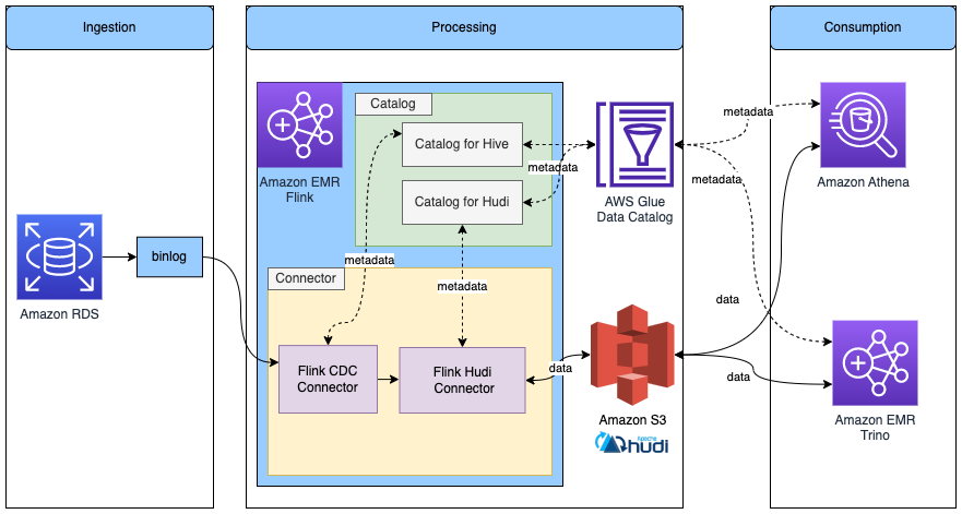
Let’s begin with a big picture: a data lake solves a variety of analytics and ML use cases dealing with internal and external data producers and consumers. The following diagram represents a generic data lake architecture. To ingest data from operational databases to an Amazon Simple Storage Service (Amazon S3) staging bucket of the data lake, either AWS Database Migration Service (AWS DMS) or any AWS partner solution from AWS Marketplace that has support for change data capture (CDC) can fulfill the requirement. AWS Glue is used to create source-aligned and consumer-aligned datasets and separate AWS Glue jobs to do feature engineering part of ML engineering and operations. Amazon Athena is used for interactive querying and AWS Lake Formation is used for access controls.

Data Lake Reference Architecture

Operational data processing framework

The operational data processing (ODP) framework contains three components: File Manager, File Processor, and Configuration Manager. Each component runs independently to solve a portion of the operational data processing use case. We have open-sourced this framework on GitHub—you can clone the code repo and inspect it while we walk you through the design and implementation of the framework components. The source code is organized in three folders, one for each component, and if you customize and adopt this framework for your use case, we recommend promoting these folders as separate code repositories in your version control system. Consider using the following repository names:

  1. aws-glue-hudi-odp-framework-file-manager
  2. aws-glue-hudi-odp-framework-file-processor
  3. aws-glue-hudi-odp-framework-config-manager

With this modular approach, you can independently deploy the components to your data lake environment by following your preferred CI/CD processes. As illustrated in the preceding diagram, these components are deployed in conjunction with a CDC solution.

Component 1: File Manager

File Manager detects files emitted by a CDC process such as AWS DMS and tracks them in an Amazon DynamoDB table. As shown in the following diagram, it consists of an Amazon EventBridge event rule, an Amazon Simple Queue Service (Amazon SQS) queue, an AWS Lambda function, and a DynamoDB table. The EventBridge rule uses Amazon S3 Event Notifications to detect the arrival of CDC files in the S3 bucket. The event rule forwards the object event notifications to the SQS queue as messages. The File Manager Lambda function consumes those messages, parses the metadata, and inserts the metadata to the DynamoDB table odpf_file_tracker. These records will then be processed by File Processor, which we discuss in the next section.

ODPF Component: File Manager

Component 2: File Processor

File Processor is the workhorse of the ODP framework. It processes files from the S3 staging bucket, creates source-aligned datasets in the raw S3 bucket, and adds or updates metadata for the datasets (AWS Glue tables) in the AWS Glue Data Catalog.

We use the following terminology when discussing File Processor:

  1. Refresh cadence – This represents the data ingestion frequency (for example, 10 minutes). It usually goes with AWS Glue worker type (one of G.1X, G.2X, G.4X, G.8X, G.025X, and so on) and batch size.
  2. Table configuration – This includes the Hudi configuration (primary key, partition key, pre-combined key, and table type (Copy on Write or Merge on Read)), table data storage mode (historical or current snapshot), S3 bucket used to store source-aligned datasets, AWS Glue database name, AWS Glue table name, and refresh cadence.
  3. Batch size – This numeric value is used to split tables into smaller batches and process their respective CDC files in parallel. For example, a configuration of 50 tables with a 10-minute refresh cadence and a batch size of 5 results in a total of 10 AWS Glue job runs, each processing CDC files for 5 tables.
  4. Table data storage mode – There are two options:
    • Historical – This table in the data lake stores historical updates to records (always append).
    • Current snapshot – This table in the data lake stores latest versioned records (upserts) with the ability to use Hudi time travel for historical updates.
  5. File processing state machine – It processes CDC files that belong to tables that share a common refresh cadence.
  6. EventBridge rule association with the file processing state machine – We use a dedicated EventBridge rule for each refresh cadence with the file processing state machine as target.
  7. File processing AWS Glue job – This is a configuration-driven AWS Glue extract, transform, and load (ETL) job that processes CDC files for one or more tables.

File Processor is implemented as a state machine using AWS Step Functions. Let’s use an example to understand this. The following diagram illustrates running File Processor state machine with a configuration that includes 18 operational tables, a refresh cadence of 10 minutes, a batch size of 5, and an AWS Glue worker type of G.1X.

ODP framework component: File Processor

The workflow includes the following steps:

  1. The EventBridge rule triggers the File Processor state machine every 10 minutes.
  2. Being the first state in the state machine, the Batch Manager Lambda function reads configurations from DynamoDB tables.
  3. The Lambda function creates four batches: three of them will be mapped to five operational tables each, and the fourth one is mapped to three operational tables. Then it feeds the batches to the Step Functions Map state.
  4. For each item in the Map state, the File Processor Trigger Lambda function will be invoked, which in turn runs the File Processor AWS Glue job.
  5. Each AWS Glue job performs the following actions:
    • Checks the status of an operational table and acquires a lock when it is not processed by any other job. The odpf_file_processing_tracker DynamoDB table is used for this purpose. When a lock is acquired, it inserts a record in the DynamoDB table with the status updating_table for the first time; otherwise, it updates the record.
    • Processes the CDC files for the given operational table from the S3 staging bucket and creates a source-aligned dataset in the S3 raw bucket. It also updates technical metadata in the AWS Glue Data Catalog.
    • Updates the status of the operational table to completed in the odpf_file_processing_tracker table. In case of processing errors, it updates the status to refresh_error and logs the stack trace.
    • It also inserts this record into the odpf_file_processing_tracker_history DynamoDB table along with additional details such as insert, update, and delete row counts.
    • Moves the records that belong to successfully processed CDC files from odpf_file_tracker to the odpf_file_tracker_history table with file_ingestion_status set to raw_file_processed.
    • Moves to the next operational table in the given batch.
    • Note: a failure to process CDC files for one of the operational tables of a given batch does not impact the processing of other operational tables.

Component 3: Configuration Manager

Configuration Manager is used to insert configuration details to the odpf_batch_config and odpf_raw_table_config tables. To keep this post concise, we provide two architecture patterns in the code repo and leave the implementation details to you.

Solution overview

Let’s test the ODP framework by replicating data from 18 operational tables to a data lake and creating source-aligned datasets with 10-minute refresh cadence. We use Amazon Relational Database Service (Amazon RDS) for MySQL to set up an operational database with 18 tables, upload the New York City Taxi – Yellow Trip Data dataset, set up AWS DMS to replicate data to Amazon S3, process the files using the framework, and finally validate the data using Amazon Athena.

Create S3 buckets

For instructions on creating an S3 bucket, refer to Creating a bucket. For this post, we create the following buckets:

  1. odpf-demo-staging-EXAMPLE-BUCKET – You will use this to migrate operational data using AWS DMS
  2. odpf-demo-raw-EXAMPLE-BUCKET – You will use this to store source-aligned datasets
  3. odpf-demo-code-artifacts-EXAMPLE-BUCKET – You will use this to store code artifacts

Deploy File Manager and File Processor

Deploy File Manager and File Processor by following instructions from this README and this README, respectively.

Set up Amazon RDS for MySQL

Complete the following steps to set up Amazon RDS for MySQL as the operational data source:

  1. Provision Amazon RDS for MySQL. For instructions, refer to Create and Connect to a MySQL Database with Amazon RDS.
  2. Connect to the database instance using MySQL Workbench or DBeaver.
  3. Create a database (schema) by running the SQL command CREATE DATABASE taxi_trips;.
  4. Create 18 tables by running the SQL commands in the ops_table_sample_ddl.sql script.

Populate data to the operational data source

Complete the following steps to populate data to the operational data source:

  1. To download the New York City Taxi – Yellow Trip Data dataset for January 2021 (Parquet file), navigate to NYC TLC Trip Record Data, expand 2021, and choose Yellow Taxi Trip records. A file called yellow_tripdata_2021-01.parquet will be downloaded to your computer.
  2. On the Amazon S3 console, open the bucket odpf-demo-staging-EXAMPLE-BUCKET and create a folder called nyc_yellow_trip_data.
  3. Upload the yellow_tripdata_2021-01.parquet file to the folder.
  4. Navigate to the bucket odpf-demo-code-artifacts-EXAMPLE-BUCKET and create a folder called glue_scripts.
  5. Download the file load_nyc_taxi_data_to_rds_mysql.py from the GitHub repo and upload it to the folder.
  6. Create an AWS Identity and Access Management (IAM) policy called load_nyc_taxi_data_to_rds_mysql_s3_policy. For instructions, refer to Creating policies using the JSON editor. Use the odpf_setup_test_data_glue_job_s3_policy.json policy definition.
  7. Create an IAM role called load_nyc_taxi_data_to_rds_mysql_glue_role. Attach the policy created in the previous step.
  8. On the AWS Glue console, create a connection for Amazon RDS for MySQL. For instructions, refer to Adding a JDBC connection using your own JDBC drivers and Setting up a VPC to connect to Amazon RDS data stores over JDBC for AWS Glue. Name the connection as odpf_demo_rds_connection.
  9. In the navigation pane of the AWS Glue console, choose Glue ETL jobs, Python Shell script editor, and Upload and edit an existing script under Options.
  10. Choose the file load_nyc_taxi_data_to_rds_mysql.py and choose Create.
  11. Complete the following steps to create your job:
    • Provide a name for the job, such as load_nyc_taxi_data_to_rds_mysql.
    • For IAM role, choose load_nyc_taxi_data_to_rds_mysql_glue_role.
    • Set Data processing units to 1/16 DPU.
    • Under Advanced properties, Connections, select the connection you created earlier.
    • Under Job parameters, add the following parameters:
      • input_sample_data_path = s3://odpf-demo-staging-EXAMPLE-BUCKET/nyc_yellow_trip_data/yellow_tripdata_2021-01.parquet
      • schema_name = taxi_trips
      • table_name = table_1
      • rds_connection_name = odpf_demo_rds_connection
    • Choose Save.
  12. On the Actions menu, run the job.
  13. Go back to your MySQL Workbench or DBeaver and validate the record count by running the SQL command select count(1) row_count from taxi_trips.table_1. You will get an output of 1369769.
  14. Populate the remaining 17 tables by running the SQL commands from the populate_17_ops_tables_rds_mysql.sql script.
  15. Get the row count from the 18 tables by running the SQL commands from the ops_data_validation_query_rds_mysql.sql script. The following screenshot shows the output.
    Record volumes (for 18 Tables) in Operational Database

Configure DynamoDB tables

Complete the following steps to configure the DynamoDB tables:

  1. Download file load_ops_table_configs_to_ddb.py from the GitHub repo and upload it to the folder glue_scripts in the S3 bucket odpf-demo-code-artifacts-EXAMPLE-BUCKET.
  2. Create an IAM policy called load_ops_table_configs_to_ddb_ddb_policy. Use the odpf_setup_test_data_glue_job_ddb_policy.json policy definition.
  3. Create an IAM role called load_ops_table_configs_to_ddb_glue_role. Attach the policy created in the previous step.
  4. On the AWS Glue console, choose Glue ETL jobs, Python Shell script editor, and Upload and edit an existing script under Options.
  5. Choose the file load_ops_table_configs_to_ddb.py and choose Create.
  6. Complete the following steps to create a job:
    • Provide a name, such as load_ops_table_configs_to_ddb.
    • For IAM role, choose load_ops_table_configs_to_ddb_glue_role.
    • Set Data processing units to 1/16 DPU.
    • Under Job parameters, add the following parameters
      • batch_config_ddb_table_name = odpf_batch_config
      • raw_table_config_ddb_table_name = odpf_demo_taxi_trips_raw
      • aws_region = e.g., us-west-1
    • Choose Save.
  7. On the Actions menu, run the job.
  8. On the DynamoDB console, get the item count from the tables. You will find 1 item in the odpf_batch_config table and 18 items in the odpf_demo_taxi_trips_raw table.

Set up a database in AWS Glue

Complete the following steps to create a database:

  1. On the AWS Glue console, under Data catalog in the navigation pane, choose Databases.
  2. Create a database called odpf_demo_taxi_trips_raw.

Set up AWS DMS for CDC

Complete the following steps to set up AWS DMS for CDC:

  1. Create an AWS DMS replication instance. For Instance class, choose dms.t3.medium.
  2. Create a source endpoint for Amazon RDS for MySQL.
  3. Create target endpoint for Amazon S3. To configure the S3 endpoint settings, use the JSON definition from dms_s3_endpoint_setting.json.
  4. Create an AWS DMS task.
    • Use the source and target endpoints created in the previous steps.
    • To create AWS DMS task mapping rules, use the JSON definition from dms_task_mapping_rules.json.
    • Under Migration task startup configuration, select Automatically on create.
  5. When the AWS DMS task starts running, you will see a task summary similar to the following screenshot.
    DMS Task Summary
  6. In the Table statistics section, you will see an output similar to the following screenshot. Here, the Full load rows and Total rows columns are important metrics whose counts should match with the record volumes of the 18 tables in the operational data source.
    DMS Task Statistics
  7. As a result of successful full load completion, you will find Parquet files in the S3 staging bucket—one Parquet file per table in a dedicated folder, similar to the following screenshot. Similarly, you will find 17 such folders in the bucket.
    DMS Output in S3 Staging Bucket for Table 1

File Manager output

The File Manager Lambda function consumes messages from the SQS queue, extracts metadata for the CDC files, and inserts one item per file to the odpf_file_tracker DynamoDB table. When you check the items, you will find 18 items with file_ingestion_status set to raw_file_landed, as shown in the following screenshot.

CDC Files in File Tracker DynamoDB Table

File Processor output

  1. On the subsequent tenth minute (since the activation of the EventBridge rule), the event rule triggers the File Processor state machine. On the Step Functions console, you will notice that the state machine is invoked, as shown in the following screenshot.
    File Processor State Machine Run Summary
  2. As shown in the following screenshot, the Batch Generator Lambda function creates four batches and constructs a Map state for parallel running of the File Processor Trigger Lambda function.
    File Processor State Machine Run Details
  3. Then, the File Processor Trigger Lambda function runs the File Processor Glue Job, as shown in the following screenshot.
    File Processor Glue Job Parallel Runs
  4. Then, you will notice that the File Processor Glue Job runs create source-aligned datasets in Hudi format in the S3 raw bucket. For Table 1, you will see an output similar to the following screenshot. There will be 17 such folders in the S3 raw bucket.
    Data in S3 raw bucket
  5. Finally, in AWS Glue Data Catalog, you will notice 18 tables created in the odpf_demo_taxi_trips_raw database, similar to the following screenshot.
    Tables in Glue Database

Data validation

Complete the following steps to validate the data:

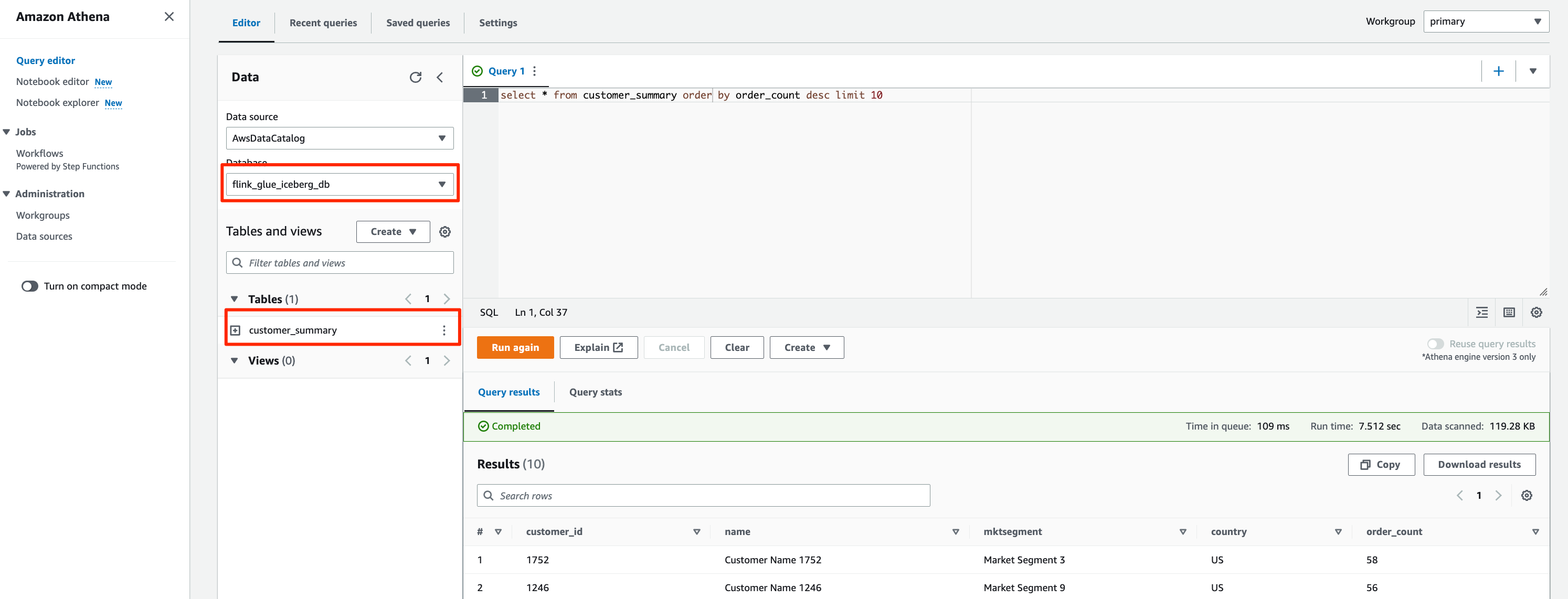
  1. On the Amazon Athena console, open the query editor, and select a workgroup or create a new workgroup.
  2. Choose AwsDataCatalog for Data source and odpf_demo_taxi_trips_raw for Database.
  3. Run the raw_data_validation_query_athena.sql SQL query. You will get an output similar to the following screenshot.
    Raw Data Validation via Amazon Athena

Validation summary: The counts in Amazon Athena match with the counts of the operational tables and it proves that the ODP framework has processed all the files and records successfully. This concludes the demo. To test additional scenarios, refer to Extended Testing in the code repo.

Outcomes

Let’s review how the ODP framework addressed the aforementioned requirements.

  1. As discussed earlier in this post, by logically grouping tables by refresh cadence and associating them to EventBridge rules, we ensured that the source-aligned tables are refreshed by the File Processor AWS Glue jobs. With the AWS Glue worker type configuration setting, we selected the appropriate compute resources while running the AWS Glue jobs (the instances of the AWS Glue job).
  2. By applying table-specific configurations (from odpf_batch_config and odpf_raw_table_config) dynamically, we were able to use one AWS Glue job to process CDC files for 18 tables.
  3. You can use this framework to support a variety of data migration use cases that require quicker data migration from on-premises storage systems to data lakes or analytics platforms on AWS. You can reuse File Manager as is and customize File Processor to work with other storage frameworks such as Apache Iceberg, Delta Lake, and purpose-built data stores such as Amazon Aurora and Amazon Redshift.
  4. To understand how the ODP framework met the company’s disaster recovery (DR) design criterion, we first need to understand the DR architecture strategy at a high level. The DR architecture strategy has the following aspects:
    • One AWS account and two AWS Regions are used for primary and secondary environments.
    • The data lake infrastructure in the secondary Region is kept in sync with the one in the primary Region.
    • Data is stored in S3 buckets, metadata data is stored in the AWS Glue Data Catalog, and access controls in Lake Formation are replicated from the primary to secondary Region.
    • The data lake source and target systems have their respective DR environments.
    • CI/CD tooling (version control, CI server, and so on) are to be made highly available.
    • The DevOps team needs to be able to deploy CI/CD pipelines of analytics frameworks (such as this ODP framework) to either the primary or secondary Region.
    • As you can imagine, disaster recovery on AWS is a vast subject, so we keep our discussion to the last design aspect.

By designing the ODP framework with three components and externalizing operational table configurations to DynamoDB global tables, the company was able to deploy the framework components to the secondary Region (in the rare event of a single-Region failure) and continue to process CDC files from the point it last processed in the primary Region. Because the CDC file tracking and processing audit data is replicated to the DynamoDB replica tables in the secondary Region, the File Manager microservice and File Processor can seamlessly run.

Clean up

When you’re finished testing this framework, you can delete the provisioned AWS resources to avoid any further charges.

Conclusion

In this post, we took a real-world operational data processing use case and presented you the framework we developed at AWS ProServe. We hope this post and the operational data processing framework using AWS Glue and Apache Hudi will expedite your journey in integrating operational databases into your modern data platforms built on AWS.


About the authors

Ravi-IthaRavi Itha is a Principal Consultant at AWS Professional Services with specialization in data and analytics and generalist background in application development. Ravi helps customers with enterprise data strategy initiatives across insurance, airlines, pharmaceutical, and financial services industries. In his 6-year tenure at Amazon, Ravi has helped the AWS builder community by publishing approximately 15 open-source solutions (accessible via GitHub handle), four blogs, and reference architectures. Outside of work, he is passionate about reading India Knowledge Systems and practicing Yoga Asanas.

srinivas-kandiSrinivas Kandi is a Data Architect at AWS Professional Services. He leads customer engagements related to data lakes, analytics, and data warehouse modernizations. He enjoys reading history and civilizations.

Create an Apache Hudi-based near-real-time transactional data lake using AWS DMS, Amazon Kinesis, AWS Glue streaming ETL, and data visualization using Amazon QuickSight

Post Syndicated from Raj Ramasubbu original https://aws.amazon.com/blogs/big-data/create-an-apache-hudi-based-near-real-time-transactional-data-lake-using-aws-dms-amazon-kinesis-aws-glue-streaming-etl-and-data-visualization-using-amazon-quicksight/

With the rapid growth of technology, more and more data volume is coming in many different formats—structured, semi-structured, and unstructured. Data analytics on operational data at near-real time is becoming a common need. Due to the exponential growth of data volume, it has become common practice to replace read replicas with data lakes to have better scalability and performance. In most real-world use cases, it’s important to replicate the data from the relational database source to the target in real time. Change data capture (CDC) is one of the most common design patterns to capture the changes made in the source database and reflect them to other data stores.

We recently announced support for streaming extract, transform, and load (ETL) jobs in AWS Glue version 4.0, a new version of AWS Glue that accelerates data integration workloads in AWS. AWS Glue streaming ETL jobs continuously consume data from streaming sources, clean and transform the data in-flight, and make it available for analysis in seconds. AWS also offers a broad selection of services to support your needs. A database replication service such as AWS Database Migration Service (AWS DMS) can replicate the data from your source systems to Amazon Simple Storage Service (Amazon S3), which commonly hosts the storage layer of the data lake. Although it’s straightforward to apply updates on a relational database management system (RDBMS) that backs an online source application, it’s difficult to apply this CDC process on your data lakes. Apache Hudi, an open-source data management framework used to simplify incremental data processing and data pipeline development, is a good option to solve this problem.

This post demonstrates how to apply CDC changes from Amazon Relational Database Service (Amazon RDS) or other relational databases to an S3 data lake, with flexibility to denormalize, transform, and enrich the data in near-real time.

Solution overview

We use an AWS DMS task to capture near-real-time changes in the source RDS instance, and use Amazon Kinesis Data Streams as a destination of the AWS DMS task CDC replication. An AWS Glue streaming job reads and enriches changed records from Kinesis Data Streams and performs an upsert into the S3 data lake in Apache Hudi format. Then we can query the data with Amazon Athena visualize it in Amazon QuickSight. AWS Glue natively supports continuous write operations for streaming data to Apache Hudi-based tables.

The following diagram illustrates the architecture used for this post, which is deployed through an AWS CloudFormation template.

Prerequisites

Before you get started, make sure you have the following prerequisites:

Source data overview

To illustrate our use case, we assume a data analyst persona who is interested in analyzing near-real-time data for sport events using the table ticket_activity. An example of this table is shown in the following screenshot.

Apache Hudi connector for AWS Glue

For this post, we use AWS Glue 4.0, which already has native support for the Hudi framework. Hudi, an open-source data lake framework, simplifies incremental data processing in data lakes built on Amazon S3. It enables capabilities including time travel queries, ACID (Atomicity, Consistency, Isolation, Durability) transactions, streaming ingestion, CDC, upserts, and deletes.

Set up resources with AWS CloudFormation

This post includes a CloudFormation template for a quick setup. You can review and customize it to suit your needs.

The CloudFormation template generates the following resources:

  • An RDS database instance (source).
  • An AWS DMS replication instance, used to replicate the data from the source table to Kinesis Data Streams.
  • A Kinesis data stream.
  • Four AWS Glue Python shell jobs:
    • rds-ingest-rds-setup-<CloudFormation Stack name> – creates one source table called ticket_activity on Amazon RDS.
    • rds-ingest-data-initial-<CloudFormation Stack name> – Sample data is automatically generated at random by the Faker library and loaded to the ticket_activity table.
    • rds-ingest-data-incremental-<CloudFormation Stack name> – Ingests new ticket activity data into the source table ticket_activity continuously. This job simulates customer activity.
    • rds-upsert-data-<CloudFormation Stack name> – Upserts specific records in the source table ticket_activity. This job simulates administrator activity.
  • AWS Identity and Access Management (IAM) users and policies.
  • An Amazon VPC, a public subnet, two private subnets, internet gateway, NAT gateway, and route tables.
    • We use private subnets for the RDS database instance and AWS DMS replication instance.
    • We use the NAT gateway to have reachability to pypi.org to use the MySQL connector for Python from the AWS Glue Python shell jobs. It also provides reachability to Kinesis Data Streams and an Amazon S3 API endpoint

To set up these resources, you must have the following prerequisites:

The following diagram illustrates the architecture of our provisioned resources.

To launch the CloudFormation stack, complete the following steps:

  1. Sign in to the AWS CloudFormation console.
  2. Choose Launch Stack
  3. Choose Next.
  4. For S3BucketName, enter the name of your new S3 bucket.
  5. For VPCCIDR, enter a CIDR IP address range that doesn’t conflict with your existing networks.
  6. For PublicSubnetCIDR, enter the CIDR IP address range within the CIDR you gave for VPCCIDR.
  7. For PrivateSubnetACIDR and PrivateSubnetBCIDR, enter the CIDR IP address range within the CIDR you gave for VPCCIDR.
  8. For SubnetAzA and SubnetAzB, choose the subnets you want to use.
  9. For DatabaseUserName, enter your database user name.
  10. For DatabaseUserPassword, enter your database user password.
  11. Choose Next.
  12. On the next page, choose Next.
  13. Review the details on the final page and select I acknowledge that AWS CloudFormation might create IAM resources with custom names.
  14. Choose Create stack.

Stack creation can take about 20 minutes.

Set up an initial source table

The AWS Glue job rds-ingest-rds-setup-<CloudFormation stack name> creates a source table called event on the RDS database instance. To set up the initial source table in Amazon RDS, complete the following steps:

  1. On the AWS Glue console, choose Jobs in the navigation pane.
  2. Choose rds-ingest-rds-setup-<CloudFormation stack name> to open the job.
  3. Choose Run.
  4. Navigate to the Runs tab and wait for Run status to show as SUCCEEDED.

This job will only create the one table, ticket_activity, in the MySQL instance (DDL). See the following code:

CREATE TABLE ticket_activity (
ticketactivity_id INT NOT NULL AUTO_INCREMENT PRIMARY KEY,
sport_type VARCHAR(256) NOT NULL,
start_date DATETIME NOT NULL,
location VARCHAR(256) NOT NULL,
seat_level VARCHAR(256) NOT NULL,
seat_location VARCHAR(256) NOT NULL,
ticket_price INT NOT NULL,
customer_name VARCHAR(256) NOT NULL,
email_address VARCHAR(256) NOT NULL,
created_at DATETIME NOT NULL,
updated_at DATETIME NOT NULL )

Ingest new records

In this section, we detail the steps to ingest new records. Implement following steps to star the execution of the jobs.

Start data ingestion to Kinesis Data Streams using AWS DMS

To start data ingestion from Amazon RDS to Kinesis Data Streams, complete the following steps:

  1. On the AWS DMS console, choose Database migration tasks in the navigation pane.
  2. Select the task rds-to-kinesis-<CloudFormation stack name>.
  3. On the Actions menu, choose Restart/Resume.
  4. Wait for the status to show as Load complete and Replication ongoing.

The AWS DMS replication task ingests data from Amazon RDS to Kinesis Data Streams continuously.

Start data ingestion to Amazon S3

Next, to start data ingestion from Kinesis Data Streams to Amazon S3, complete the following steps:

  1. On the AWS Glue console, choose Jobs in the navigation pane.
  2. Choose streaming-cdc-kinesis2hudi-<CloudFormation stack name> to open the job.
  3. Choose Run.

Do not stop this job; you can check the run status on the Runs tab and wait for it to show as Running.

Start the data load to the source table on Amazon RDS

To start data ingestion to the source table on Amazon RDS, complete the following steps:

  1. On the AWS Glue console, choose Jobs in the navigation pane.
  2. Choose rds-ingest-data-initial-<CloudFormation stack name> to open the job.
  3. Choose Run.
  4. Navigate to the Runs tab and wait for Run status to show as SUCCEEDED.

Validate the ingested data

After about 2 minutes from starting the job, the data should be ingested into the Amazon S3. To validate the ingested data in the Athena, complete the following steps:

  1. On the Athena console, complete the following steps if you’re running an Athena query for the first time:
    • On the Settings tab, choose Manage.
    • Specify the stage directory and the S3 path where Athena saves the query results.
    • Choose Save.

  1. On the Editor tab, run the following query against the table to check the data:
SELECT * FROM "database_<account_number>_hudi_cdc_demo"."ticket_activity" limit 10;

Note that AWS Cloud Formation will create the database with the account number as database_<your-account-number>_hudi_cdc_demo.

Update existing records

Before you update the existing records, note down the ticketactivity_id value of a record from the ticket_activity table. Run the following SQL using Athena. For this post, we use ticketactivity_id = 46 as an example:

SELECT * FROM "database_<account_number>_hudi_cdc_demo"."ticket_activity" limit 10;

To simulate a real-time use case, update the data in the source table ticket_activity on the RDS database instance to see that the updated records are replicated to Amazon S3. Complete the following steps:

  1. On the AWS Glue console, choose Jobs in the navigation pane.
  2. Choose rds-ingest-data-incremental-<CloudFormation stack name> to open the job.
  3. Choose Run.
  4. Choose the Runs tab and wait for Run status to show as SUCCEEDED.

To upsert the records in the source table, complete the following steps:

  1. On the AWS Glue console, choose Jobs in the navigation pane.
  2. Choose the job rds-upsert-data-<CloudFormation stack name>.
  3. On the Job details tab, under Advanced properties, for Job parameters, update the following parameters:
    • For Key, enter --ticketactivity_id.
    • For Value, replace 1 with one of the ticket IDs you noted above (for this post, 46).

  1. Choose Save.
  2. Choose Run and wait for the Run status to show as SUCCEEDED.

This AWS Glue Python shell job simulates a customer activity to buy a ticket. It updates a record in the source table ticket_activity on the RDS database instance using the ticket ID passed in the job argument --ticketactivity_id. It will update ticket_price=500 and updated_at with the current timestamp.

To validate the ingested data in Amazon s3, run the same query from Athena and check the ticket_activity value you noted earlier to observe the ticket_price and updated_at fields:

SELECT * FROM "database_<account_number>_hudi_cdc_demo"."ticket_activity" where ticketactivity_id = 46 ;

Visualize the data in QuickSight

After you have the output file generated by the AWS Glue streaming job in the S3 bucket, you can use QuickSight to visualize the Hudi data files. QuickSight is a scalable, serverless, embeddable, ML-powered business intelligence (BI) service built for the cloud. QuickSight lets you easily create and publish interactive BI dashboards that include ML-powered insights. QuickSight dashboards can be accessed from any device and seamlessly embedded into your applications, portals, and websites.

Build a QuickSight dashboard

To build a QuickSight dashboard, complete the following steps:

  1. Open the QuickSight console.

You’re presented with the QuickSight welcome page. If you haven’t signed up for QuickSight, you may have to complete the signup wizard. For more information, refer to Signing up for an Amazon QuickSight subscription.

After you have signed up, QuickSight presents a “Welcome wizard.” You can view the short tutorial, or you can close it.

  1. On the QuickSight console, choose your user name and choose Manage QuickSight.
  2. Choose Security & permissions, then choose Manage.
  3. Select Amazon S3 and select the buckets that you created earlier with AWS CloudFormation.
  4. Select Amazon Athena.
  5. Choose Save.
  6. If you changed your Region during the first step of this process, change it back to the Region that you used earlier during the AWS Glue jobs.

Create a dataset

Now that you have QuickSight up and running, you can create your dataset. Complete the following steps:

  1. On the QuickSight console, choose Datasets in the navigation pane.
  2. Choose New dataset.
  3. Choose Athena.
  4. For Data source name, enter a name (for example, hudi-blog).
  5. Choose Validate.
  6. After the validation is successful, choose Create data source.
  7. For Database, choose database_<your-account-number>_hudi_cdc_demo.
  8. For Tables, select ticket_activity.
  9. Choose Select.
  10. Choose Visualize.
  11. Choose hour and then ticket_activity_id to get the count of ticket_activity_id by hour.

Clean up

To clean up your resources, complete the following steps:

  1. Stop the AWS DMS replication task rds-to-kinesis-<CloudFormation stack name>.
  2. Navigate to the RDS database and choose Modify.
  3. Deselect Enable deletion protection, then choose Continue.
  4. Stop the AWS Glue streaming job streaming-cdc-kinesis2redshift-<CloudFormation stack name>.
  5. Delete the CloudFormation stack.
  6. On the QuickSight dashboard, choose your user name, then choose Manage QuickSight.
  7. Choose Account settings, then choose Delete account.
  8. Choose Delete account to confirm.
  9. Enter confirm and choose Delete account.

Conclusion

In this post, we demonstrated how you can stream data—not only new records, but also updated records from relational databases—to Amazon S3 using an AWS Glue streaming job to create an Apache Hudi-based near-real-time transactional data lake. With this approach, you can easily achieve upsert use cases on Amazon S3. We also showcased how to visualize the Apache Hudi table using QuickSight and Athena. As a next step, refer to the Apache Hudi performance tuning guide for a high-volume dataset. To learn more about authoring dashboards in QuickSight, check out the QuickSight Author Workshop.


About the Authors

Raj Ramasubbu is a Sr. Analytics Specialist Solutions Architect focused on big data and analytics and AI/ML with Amazon Web Services. He helps customers architect and build highly scalable, performant, and secure cloud-based solutions on AWS. Raj provided technical expertise and leadership in building data engineering, big data analytics, business intelligence, and data science solutions for over 18 years prior to joining AWS. He helped customers in various industry verticals like healthcare, medical devices, life science, retail, asset management, car insurance, residential REIT, agriculture, title insurance, supply chain, document management, and real estate.

Rahul Sonawane is a Principal Analytics Solutions Architect at AWS with AI/ML and Analytics as his area of specialty.

Sundeep Kumar is a Sr. Data Architect, Data Lake at AWS, helping customers build data lake and analytics platform and solutions. When not building and designing data lakes, Sundeep enjoys listening music and playing guitar.

Build a data lake with Apache Flink on Amazon EMR

Post Syndicated from Jianwei Li original https://aws.amazon.com/blogs/big-data/build-a-unified-data-lake-with-apache-flink-on-amazon-emr/

To build a data-driven business, it is important to democratize enterprise data assets in a data catalog. With a unified data catalog, you can quickly search datasets and figure out data schema, data format, and location. The AWS Glue Data Catalog provides a uniform repository where disparate systems can store and find metadata to keep track of data in data silos.

Apache Flink is a widely used data processing engine for scalable streaming ETL, analytics, and event-driven applications. It provides precise time and state management with fault tolerance. Flink can process bounded stream (batch) and unbounded stream (stream) with a unified API or application. After data is processed with Apache Flink, downstream applications can access the curated data with a unified data catalog. With unified metadata, both data processing and data consuming applications can access the tables using the same metadata.

This post shows you how to integrate Apache Flink in Amazon EMR with the AWS Glue Data Catalog so that you can ingest streaming data in real time and access the data in near-real time for business analysis.

Apache Flink connector and catalog architecture

Apache Flink uses a connector and catalog to interact with data and metadata. The following diagram shows the architecture of the Apache Flink connector for data read/write, and catalog for metadata read/write.

Flink Glue Architecture

For data read/write, Flink has the interface DynamicTableSourceFactory for read and DynamicTableSinkFactory for write. A different Flink connector implements two interfaces to access data in different storage. For example, the Flink FileSystem connector has FileSystemTableFactory to read/write data in Hadoop Distributed File System (HDFS) or Amazon Simple Storage Service (Amazon S3), the Flink HBase connector has HBase2DynamicTableFactory to read/write data in HBase, and the Flink Kafka connector has KafkaDynamicTableFactory to read/write data in Kafka. You can refer to Table & SQL Connectors for more information.

For metadata read/write, Flink has the catalog interface. Flink has three built-in implementations for the catalog. GenericInMemoryCatalog stores the catalog data in memory. JdbcCatalog stores the catalog data in a JDBC-supported relational database. As of this writing, MySQL and PostgreSQL databases are supported in the JDBC catalog. HiveCatalog stores the catalog data in Hive Metastore. HiveCatalog uses HiveShim to provide different Hive version compatibility. We can configure different metastore clients to use Hive Metastore or the AWS Glue Data Catalog. In this post, we configure the Amazon EMR property hive.metastore.client.factory.class to com.amazonaws.glue.catalog.metastore.AWSGlueDataCatalogHiveClientFactory (see Using the AWS Glue Data Catalog as the metastore for Hive) so that we can use the AWS Glue Data Catalog to store Flink catalog data. Refer to Catalogs for more information.

Most Flink built-in connectors, such as for Kafka, Amazon Kinesis, Amazon DynamoDB, Elasticsearch, or FileSystem, can use Flink HiveCatalog to store metadata in the AWS Glue Data Catalog. However, some connector implementations such as Apache Iceberg have their own catalog management mechanism. FlinkCatalog in Iceberg implements the catalog interface in Flink. FlinkCatalog in Iceberg has a wrapper to its own catalog implementation. The following diagram shows the relationship between Apache Flink, the Iceberg connector, and the catalog. For more information, refer to Creating catalogs and using catalogs and Catalogs.

Flink Iceberg Glue Architecture

Apache Hudi also has its own catalog management. Both HoodieCatalog and HoodieHiveCatalog implements a catalog interface in Flink. HoodieCatalog stores metadata in a file system such as HDFS. HoodieHiveCatalog stores metadata in Hive Metastore or the AWS Glue Data Catalog, depending on whether you configure hive.metastore.client.factory.class to use com.amazonaws.glue.catalog.metastore.AWSGlueDataCatalogHiveClientFactory. The following diagram shows relationship between Apache Flink, the Hudi connector, and the catalog. For more information, refer to Create Catalog.

Flink Hudi Glue Architecture

Because Iceberg and Hudi have different catalog management mechanisms, we show three scenarios of Flink integration with the AWS Glue Data Catalog in this post:

  • Read/Write to Iceberg tables in Flink with metadata in Glue Data Catalog
  • Read/Write to Hudi tables in Flink with metadata in Glue Data Catalog
  • Read/Write to other storage format in Flink with metadata in Glue Data Catalog

Solution overview

The following diagram shows the overall architecture of the solution described in this post.

Flink Glue Integration

In this solution, we enable an Amazon RDS for MySQL binlog to extract transaction changes in real time. The Amazon EMR Flink CDC connector reads the binlog data and processes the data. Transformed data can be stored in Amazon S3. We use the AWS Glue Data Catalog to store the metadata such as table schema and table location. Downstream data consumer applications such as Amazon Athena or Amazon EMR Trino access the data for business analysis.

The following are the high-level steps to set up this solution:

  1. Enable binlog for Amazon RDS for MySQL and initialize the database.
  2. Create an EMR cluster with the AWS Glue Data Catalog.
  3. Ingest change data capture (CDC) data with Apache Flink CDC in Amazon EMR.
  4. Store the processed data in Amazon S3 with metadata in the AWS Glue Data Catalog.
  5. Verify all table metadata is stored in the AWS Glue Data Catalog.
  6. Consume data with Athena or Amazon EMR Trino for business analysis.
  7. Update and delete source records in Amazon RDS for MySQL and validate the reflection of the data lake tables.

Prerequisites

This post uses an AWS Identity and Access Management (IAM) role with permissions for the following services:

  • Amazon RDS for MySQL (5.7.40)
  • Amazon EMR (6.9.0)
  • Amazon Athena
  • AWS Glue Data Catalog
  • Amazon S3

Enable binlog for Amazon RDS for MySQL and initialize the database

To enable CDC in Amazon RDS for MySQL, we need to configure binary logging for Amazon RDS for MySQL. Refer to Configuring MySQL binary logging for more information. We also create the database salesdb in MySQL and create the tables customer, order, and others to set up the data source.

  1. On the Amazon RDS console, choose Parameter groups in the navigation pane.
  2. Create a new parameter group for MySQL.
  3. Edit the parameter group you just created to set binlog_format=ROW.

RDS-Binlog-Format

  1. Edit the parameter group you just created to set binlog_row_image=full.

RDS-Binlog-Row-Image

  1. Create an RDS for MySQL DB instance with the parameter group.
  2. Note down the values for hostname, username, and password, which we use later.
  3. Download the MySQL database initialization script from Amazon S3 by running the following command:
aws s3 cp s3://emr-workshops-us-west-2/glue_immersion_day/scripts/salesdb.sql ./salesdb.sql
  1. Connect to the RDS for MySQL database and run the salesdb.sql command to initialize the database, providing the host name and user name according to your RDS for MySQL database configuration:
mysql -h <hostname> -u <username> -p
mysql> source salesdb.sql

Create an EMR cluster with the AWS Glue Data Catalog

From Amazon EMR 6.9.0, the Flink table API/SQL can integrate with the AWS Glue Data Catalog. To use the Flink and AWS Glue integration, you must create an Amazon EMR 6.9.0 or later version.

  1. Create the file iceberg.properties for the Amazon EMR Trino integration with the Data Catalog. When the table format is Iceberg, your file should have following content:
iceberg.catalog.type=glue
connector.name=iceberg
  1. Upload iceberg.properties to an S3 bucket, for example DOC-EXAMPLE-BUCKET.

For more information on how to integrate Amazon EMR Trino with Iceberg, refer to Use an Iceberg cluster with Trino.

  1. Create the file trino-glue-catalog-setup.sh to configure the Trino integration with the Data Catalog. Use trino-glue-catalog-setup.sh as the bootstrap script. Your file should have the following content (replace DOC-EXAMPLE-BUCKET with your S3 bucket name):
set -ex 
sudo aws s3 cp s3://DOC-EXAMPLE-BUCKET/iceberg.properties /etc/trino/conf/catalog/iceberg.properties

  1. Upload trino-glue-catalog-setup.sh to your S3 bucket (DOC-EXAMPLE-BUCKET).

Refer to Create bootstrap actions to install additional software to run a bootstrap script.

  1. Create the file flink-glue-catalog-setup.sh to configure the Flink integration with the Data Catalog.
  2. Use a script runner and run the flink-glue-catalog-setup.sh script as a step function.

Your file should have the following content (the JAR file name here is using Amazon EMR 6.9.0; a later version JAR name may change, so make sure to update according to your Amazon EMR version).

Note that here we use an Amazon EMR step, not a bootstrap, to run this script. An Amazon EMR step script is run after Amazon EMR Flink is provisioned.

set -ex

sudo cp /usr/lib/hive/auxlib/aws-glue-datacatalog-hive3-client.jar /usr/lib/flink/lib
sudo cp /usr/lib/hive/lib/antlr-runtime-3.5.2.jar /usr/lib/flink/lib
sudo cp /usr/lib/hive/lib/hive-exec.jar /lib/flink/lib
sudo cp /usr/lib/hive/lib/libfb303-0.9.3.jar /lib/flink/lib
sudo cp /usr/lib/flink/opt/flink-connector-hive_2.12-1.15.2.jar /lib/flink/lib
sudo chmod 755 /usr/lib/flink/lib/aws-glue-datacatalog-hive3-client.jar
sudo chmod 755 /usr/lib/flink/lib/antlr-runtime-3.5.2.jar
sudo chmod 755 /usr/lib/flink/lib/hive-exec.jar
sudo chmod 755 /usr/lib/flink/lib/libfb303-0.9.3.jar
sudo chmod 755 /usr/lib/flink/lib/flink-connector-hive_2.12-1.15.2.jar

sudo wget https://repo1.maven.org/maven2/com/ververica/flink-sql-connector-mysql-cdc/2.2.1/flink-sql-connector-mysql-cdc-2.2.1.jar -O /lib/flink/lib/flink-sql-connector-mysql-cdc-2.2.1.jar
sudo chmod 755 /lib/flink/lib/flink-sql-connector-mysql-cdc-2.2.1.jar

sudo ln -s /usr/share/aws/iceberg/lib/iceberg-flink-runtime.jar /usr/lib/flink/lib/
sudo ln -s /usr/lib/hudi/hudi-flink-bundle.jar /usr/lib/flink/lib/

sudo mv /usr/lib/flink/opt/flink-table-planner_2.12-1.15.2.jar /usr/lib/flink/lib/
sudo mv /usr/lib/flink/lib/flink-table-planner-loader-1.15.2.jar /usr/lib/flink/opt/
  1. Upload flink-glue-catalog-setup.sh to your S3 bucket (DOC-EXAMPLE-BUCKET).

Refer to Configuring Flink to Hive Metastore in Amazon EMR for more information on how to configure Flink and Hive Metastore. Refer to Run commands and scripts on an Amazon EMR cluster for more details on running the Amazon EMR step script.

  1. Create an EMR 6.9.0 cluster with the applications Hive, Flink, and Trino.

You can create an EMR cluster with the AWS Command Line Interface (AWS CLI) or the AWS Management Console. Refer to the appropriate subsection for instructions.

Create an EMR cluster with the AWS CLI

To use the AWS CLI, complete the following steps:

  1. Create the file emr-flink-trino-glue.json to configure Amazon EMR to use the Data Catalog. Your file should have the following content:
[
{
"Classification": "hive-site",
"Properties": {
"hive.metastore.client.factory.class": "com.amazonaws.glue.catalog.metastore.AWSGlueDataCatalogHiveClientFactory"
}
},
{
"Classification": "trino-connector-hive",
"Properties": {
"hive.metastore": "glue"
}
}
]
  1. Run the following command to create the EMR cluster. Provide your local emr-flink-trino-glue.json parent folder path, S3 bucket, EMR cluster Region, EC2 key name, and S3 bucket for EMR logs.
aws emr create-cluster --release-label emr-6.9.0 \
--applications Name=Hive Name=Flink Name=Spark Name=Trino \
--region us-west-2 \
--name flink-trino-glue-emr69 \
--configurations "file:///<your configuration path>/emr-flink-trino-glue.json" \
--bootstrap-actions '[{"Path":"s3://DOC-EXAMPLE-BUCKET/trino-glue-catalog-setup.sh","Name":"Add iceberg.properties for Trino"}]' \
--steps '[{"Args":["s3://DOC-EXAMPLE-BUCKET/flink-glue-catalog-setup.sh"],"Type":"CUSTOM_JAR","ActionOnFailure":"CONTINUE","Jar":"s3://<region>.elasticmapreduce/libs/script-runner/script-runner.jar","Properties":"","Name":"Flink-glue-integration"}]' \
--instance-groups \
InstanceGroupType=MASTER,InstanceType=m6g.2xlarge,InstanceCount=1 \
InstanceGroupType=CORE,InstanceType=m6g.2xlarge,InstanceCount=2 \
--use-default-roles \
--ebs-root-volume-size 30 \
--ec2-attributes KeyName=<keyname> \
--log-uri s3://<s3-bucket-for-emr>/elasticmapreduce/

Create an EMR cluster on the console

To use the console, complete the following steps:

  1. On the Amazon EMR console, create an EMR cluster and select Use for Hive table metadata for AWS Glue Data Catalog settings.
  2. Add configuration settings with the following code:
[
{
"Classification": "trino-connector-hive",
"Properties": {
"hive.metastore": "glue"
}
}
]

EMR-6.9-Flink-Hive-Glue-1

  1. In the Steps section, add a step called Custom JAR.
  2. Set JAR location to s3://<region>.elasticmapreduce/libs/script-runner/script-runner.jar, where <region> is the region in which your EMR cluster resides.
  3. Set Arguments to the S3 path you uploaded earlier.

EMR-6.9-Flink-Hive-Glue-2

  1. In the Bootstrap Actions section, choose Custom Action.
  2. Set Script location to the S3 path you uploaded.

EMR-6.9-Flink-Hive-Glue-3

  1. Continue the subsequent steps to complete your EMR cluster creation.

Ingest CDC data with Apache Flink CDC in Amazon EMR

The Flink CDC connector supports reading database snapshots and captures updates in the configured tables. We have deployed the Flink CDC connector for MySQL by downloading flink-sql-connector-mysql-cdc-2.2.1.jar and putting it into the Flink library when we create our EMR cluster. The Flink CDC connector can use the Flink Hive catalog to store Flink CDC table schema into Hive Metastore or the AWS Glue Data Catalog. In this post, we use the Data Catalog to store our Flink CDC table.

Complete the following steps to ingest RDS for MySQL databases and tables with Flink CDC and store metadata in the Data Catalog:

  1. SSH to the EMR primary node.
  2. Start Flink on a YARN session by running the following command, providing your S3 bucket name:
flink-yarn-session -d -jm 2048 -tm 4096 -s 2 \
-D state.backend=rocksdb \
-D state.backend.incremental=true \
-D state.checkpoint-storage=filesystem \
-D state.checkpoints.dir=s3://<flink-glue-integration-bucket>/flink-checkponts/ \
-D state.checkpoints.num-retained=10 \
-D execution.checkpointing.interval=10s \
-D execution.checkpointing.mode=EXACTLY_ONCE \
-D execution.checkpointing.externalized-checkpoint-retention=RETAIN_ON_CANCELLATION \
-D execution.checkpointing.max-concurrent-checkpoints=1
  1. Start the Flink SQL client CLI by running the following command:
/usr/lib/flink/bin/sql-client.sh embedded
  1. Create the Flink Hive catalog by specifying the catalog type as hive and providing your S3 bucket name:
CREATE CATALOG glue_catalog WITH (
'type' = 'hive',
'default-database' = 'default',
'hive-conf-dir' = '/etc/hive/conf.dist'
);
USE CATALOG glue_catalog;
CREATE DATABASE IF NOT EXISTS flink_cdc_db WITH ('hive.database.location-uri'= 's3://<flink-glue-integration-bucket>/flink-glue-for-hive/warehouse/')
use flink_cdc_db;

Because we’re configuring the EMR Hive catalog use the AWS Glue Data Catalog, all the databases and tables created in the Flink Hive catalog are stored in the Data Catalog.

  1. Create the Flink CDC table, providing the host name, user name, and password for the RDS for MySQL instance you created earlier.

Note that because the RDS for MySQL user name and password will be stored in the Data Catalog as table properties, you should be enable AWS Glue database/table authorization with AWS Lake Formation to protect your sensitive data.

CREATE TABLE `glue_catalog`.`flink_cdc_db`.`customer_cdc` (
`CUST_ID` double NOT NULL,
`NAME` STRING NOT NULL,
`MKTSEGMENT` STRING NOT NULL,
PRIMARY KEY (`CUST_ID`) NOT ENFORCED
) WITH (
'connector' = 'mysql-cdc',
'hostname' = '<hostname>',
'port' = '3306',
'username' = '<username>',
'password' = '<password>',
'database-name' = 'salesdb',
'table-name' = 'CUSTOMER'
);

CREATE TABLE `glue_catalog`.`flink_cdc_db`.`customer_site_cdc` (
`SITE_ID` double NOT NULL,
`CUST_ID` double NOT NULL,
`ADDRESS` STRING NOT NULL,
`CITY` STRING NOT NULL,
`STATE` STRING NOT NULL,
`COUNTRY` STRING NOT NULL,
`PHONE` STRING NOT NULL,
PRIMARY KEY (`SITE_ID`) NOT ENFORCED
) WITH (
'connector' = 'mysql-cdc',
'hostname' = '<hostname>',
'port' = '3306',
'username' = '<username>',
'password' = '<password>',
'database-name' = 'salesdb',
'table-name' = 'CUSTOMER_SITE'
);

CREATE TABLE `glue_catalog`.`flink_cdc_db`.`sales_order_all_cdc` (
`ORDER_ID` int NOT NULL,
`SITE_ID` double NOT NULL,
`ORDER_DATE` TIMESTAMP NOT NULL,
`SHIP_MODE` STRING NOT NULL
) WITH (
'connector' = 'mysql-cdc',
'hostname' = '<hostname>',
'port' = '3306',
'username' = '<username>',
'password' = '<password>',
'database-name' = 'salesdb',
'table-name' = 'SALES_ORDER_ALL',
'scan.incremental.snapshot.enabled' = 'FALSE'
);
  1. Query the table you just created:
SELECT count(O.ORDER_ID) AS ORDER_COUNT,
C.CUST_ID,
C.NAME,
C.MKTSEGMENT
FROM   customer_cdc C
JOIN customer_site_cdc CS
ON C.CUST_ID = CS.CUST_ID
JOIN sales_order_all_cdc O
ON O.SITE_ID = CS.SITE_ID
GROUP  BY C.CUST_ID,
C.NAME,
C.MKTSEGMENT;

You will get a query result like following screenshot.

Flink-SQL-CDC-Test

Store processed data in Amazon S3 with metadata in the Data Catalog

As we’re ingesting the relational database data in Amazon RDS for MySQL, raw data may be updated or deleted. To support data update and delete, we can choose data lake technologies such as Apache Iceberg or Apache Hudi to store the processed data. As we mentioned earlier, Iceberg and Hudi have different catalog management. We show both scenarios to use Flink to read/write the Iceberg and Hudi tables with metadata in the AWS Glue Data Catalog.

For non-Iceberg and non-Hudi, we use a FileSystem Parquet file to show how the Flink built-in connector uses the Data Catalog.

Read/Write to Iceberg tables in Flink with metadata in Glue Data Catalog

The following diagram shows the architecture for this configuration.

Flink Glue Integration for Iceberg

  1. Create a Flink Iceberg catalog using the Data Catalog by specifying catalog-impl as org.apache.iceberg.aws.glue.GlueCatalog.

For more information about Flink and Data Catalog integration for Iceberg, refer to Glue Catalog.

  1. In the Flink SQL client CLI, run the following command, providing your S3 bucket name:
CREATE CATALOG glue_catalog_for_iceberg WITH (
'type'='iceberg',
'warehouse'='s3://<flink-glue-integration-bucket>/flink-glue-for-iceberg/warehouse/',
'catalog-impl'='org.apache.iceberg.aws.glue.GlueCatalog',
'io-impl'='org.apache.iceberg.aws.s3.S3FileIO',
'lock-impl'='org.apache.iceberg.aws.glue.DynamoLockManager',
'lock.table'='FlinkGlue4IcebergLockTable' );
  1. Create an Iceberg table to store processed data:
USE CATALOG glue_catalog_for_iceberg;
CREATE DATABASE IF NOT EXISTS flink_glue_iceberg_db;
USE flink_glue_iceberg_db;
CREATE TABLE `glue_catalog_for_iceberg`.`flink_glue_iceberg_db`.`customer_summary` (
`CUSTOMER_ID` bigint,
`NAME` STRING,
`MKTSEGMENT` STRING,
`COUNTRY` STRING,
`ORDER_COUNT` BIGINT,
PRIMARY KEY (`CUSTOMER_ID`) NOT Enforced
)
WITH (
'format-version'='2',
'write.upsert.enabled'='true');
  1. Insert the processed data into Iceberg:
INSERT INTO `glue_catalog_for_iceberg`.`flink_glue_iceberg_db`.`customer_summary`
SELECT CAST(C.CUST_ID AS BIGINT) CUST_ID,
C.NAME,
C.MKTSEGMENT,
CS.COUNTRY,
count(O.ORDER_ID) AS ORDER_COUNT
FROM   `glue_catalog`.`flink_cdc_db`.`customer_cdc` C
JOIN `glue_catalog`.`flink_cdc_db`.`customer_site_cdc` CS
ON C.CUST_ID = CS.CUST_ID
JOIN `glue_catalog`.`flink_cdc_db`.`sales_order_all_cdc` O
ON O.SITE_ID = CS.SITE_ID
GROUP  BY C.CUST_ID,
C.NAME,
C.MKTSEGMENT,
CS.COUNTRY;

Read/Write to Hudi tables in Flink with metadata in Glue Data Catalog

The following diagram shows the architecture for this configuration.

Flink Glue Integration for Hudi

Complete the following steps:

  1. Create a catalog for Hudi to use the Hive catalog by specifying mode as hms.

Because we already configured Amazon EMR to use the Data Catalog when we created the EMR cluster, this Hudi Hive catalog uses the Data Catalog under the hood. For more information about Flink and Data Catalog integration for Hudi, refer to Create Catalog.

  1. In the Flink SQL client CLI, run the following command, providing your S3 bucket name:
CREATE CATALOG glue_catalog_for_hudi WITH (
'type' = 'hudi',
'mode' = 'hms',
'table.external' = 'true',
'default-database' = 'default',
'hive.conf.dir' = '/etc/hive/conf.dist',
'catalog.path' = 's3://<flink-glue-integration-bucket>/flink-glue-for-hudi/warehouse/'
);
  1. Create a Hudi table using the Data Catalog, and provide your S3 bucket name:
USE CATALOG glue_catalog_for_hudi;
CREATE DATABASE IF NOT EXISTS flink_glue_hudi_db;
use flink_glue_hudi_db;
CREATE TABLE `glue_catalog_for_hudi`.`flink_glue_hudi_db`.`customer_summary` (
`CUSTOMER_ID` bigint,
`NAME` STRING,
`MKTSEGMENT` STRING,
`COUNTRY` STRING,
`ORDER_COUNT` BIGINT,
PRIMARY KEY (`CUSTOMER_ID`) NOT Enforced
)
WITH (
'connector' = 'hudi',
'write.tasks' = '4',
'path' = 's3://<flink-glue-integration-bucket>/flink-glue-for-hudi/warehouse/customer_summary',
'table.type' = 'COPY_ON_WRITE',
'read.streaming.enabled' = 'true',
'read.streaming.check-interval' = '1'
);
  1. Insert the processed data into Hudi:
INSERT INTO `glue_catalog_for_hudi`.`flink_glue_hudi_db`.`customer_summary`
SELECT CAST(C.CUST_ID AS BIGINT) CUST_ID,
C.NAME,
C.MKTSEGMENT,
CS.COUNTRY,
count(O.ORDER_ID) AS ORDER_COUNT
FROM   `glue_catalog`.`flink_cdc_db`.`customer_cdc` C
JOIN `glue_catalog`.`flink_cdc_db`.`customer_site_cdc` CS
ON C.CUST_ID = CS.CUST_ID
JOIN `glue_catalog`.`flink_cdc_db`.`sales_order_all_cdc` O
ON O.SITE_ID = CS.SITE_ID
GROUP  BY C.CUST_ID,
C.NAME,
C.MKTSEGMENT,
CS.COUNTRY;

Read/Write to other storage format in Flink with metadata in Glue Data Catalog

The following diagram shows the architecture for this configuration.

Flink Glue Integration for Parquet

We already created the Flink Hive catalog in the previous step, so we’ll reuse that catalog.

  1. In the Flink SQL client CLI, run the following command:
USE CATALOG glue_catalog;
CREATE DATABASE IF NOT EXISTS flink_hive_parquet_db;
use flink_hive_parquet_db;

We change the SQL dialect to Hive to create a table with Hive syntax.

  1. Create a table with the following SQL, and provide your S3 bucket name:
SET table.sql-dialect=hive;

CREATE TABLE `customer_summary` (
`CUSTOMER_ID` bigint,
`NAME` STRING,
`MKTSEGMENT` STRING,
`COUNTRY` STRING,
`ORDER_COUNT` BIGINT
)
STORED AS parquet
LOCATION 's3://<flink-glue-integration-bucket>/flink-glue-for-hive-parquet/warehouse/customer_summary';

Because Parquet files don’t support updated rows, we can’t consume data from CDC data. However, we can consume data from Iceberg or Hudi.

  1. Use the following code to query the Iceberg table and insert data into the Parquet table:
SET table.sql-dialect=default;
SET execution.runtime-mode = batch;
INSERT INTO `glue_catalog`.`flink_hive_parquet_db`.`customer_summary`
SELECT * from `glue_catalog_for_iceberg`.`flink_glue_iceberg_db`.`customer_summary`;

Verify all table metadata is stored in the Data Catalog

You can navigate to the AWS Glue console to verify all the tables are stored in the Data Catalog.

  1. On the AWS Glue console, choose Databases in the navigation pane to list all the databases we created.

Glue-Databases

  1. Open a database and verify that all the tables are in that database.

Glue-Tables

Consume data with Athena or Amazon EMR Trino for business analysis

You can use Athena or Amazon EMR Trino to access the result data.

Query the data with Athena

To access the data with Athena, complete the following steps:

  1. Open the Athena query editor.
  2. Choose flink_glue_iceberg_db for Database.

You should see the customer_summary table listed.

  1. Run the following SQL script to query the Iceberg result table:
select * from customer_summary order by order_count desc limit 10

The query result will look like the following screenshot.

Athena-Iceberg-Query

  1. For the Hudi table, change Database to flink_glue_hudi_db and run the same SQL query.

Athena-Hudi-Query

  1. For the Parquet table, change Database to flink_hive_parquet_db and run the same SQL query.

Athena-Parquet-Query

Query the data with Amazon EMR Trino

To access Iceberg with Amazon EMR Trino, SSH to the EMR primary node.

  1. Run the following command to start the Trino CLI:
trino-cli --catalog iceberg

Amazon EMR Trino can now query the tables in the AWS Glue Data Catalog.

  1. Run the following command to query the result table:
show schemas;
use flink_glue_iceberg_db;
show tables;
select * from customer_summary order by order_count desc limit 10;

The query result looks like the following screenshot.

EMR-Trino-Iceberg-Query

  1. Exit the Trino CLI.
  2. Start the Trino CLI with the hive catalog to query the Hudi table:
trino-cli --catalog hive
  1. Run the following command to query the Hudi table:
show schemas;
use flink_glue_hudi_db;
show tables;
select * from customer_summary order by order_count desc limit 10;

Update and delete source records in Amazon RDS for MySQL and validate the reflection of the data lake tables

We can update and delete some records in the RDS for MySQL database and then validate that the changes are reflected in the Iceberg and Hudi tables.

  1. Connect to the RDS for MySQL database and run the following SQL:
update CUSTOMER set NAME = 'updated_name' where CUST_ID=7;

delete from CUSTOMER where CUST_ID=11;
  1. Query the customer_summary table with Athena or Amazon EMR Trino.

The updated and deleted records are reflected in the Iceberg and Hudi tables.

Athena-Iceberg-Query-Updated

Clean up

When you’re done with this exercise, complete the following steps to delete your resources and stop incurring costs:

  1. Delete the RDS for MySQL database.
  2. Delete the EMR cluster.
  3. Drop the databases and tables created in the Data Catalog.
  4. Remove files in Amazon S3.

Conclusion

This post showed you how to integrate Apache Flink in Amazon EMR with the AWS Glue Data Catalog. You can use a Flink SQL connector to read/write data in a different store, such as Kafka, CDC, HBase, Amazon S3, Iceberg, or Hudi. You can also store the metadata in the Data Catalog. The Flink table API has the same connector and catalog implementation mechanism. In a single session, we can use multiple catalog instances pointing to different types, like IcebergCatalog and HiveCatalog, and use then interchangeably in your query. You can also write code with the Flink table API to develop the same solution to integrate Flink and the Data Catalog.

In our solution, we consumed the RDS for MySQL binary log directly with Flink CDC. You can also use Amazon MSK Connect to consume the binary log with MySQL Debezim and store the data in Amazon Managed Streaming for Apache Kafka (Amazon MSK). Refer to Create a low-latency source-to-data lake pipeline using Amazon MSK Connect, Apache Flink, and Apache Hudi for more information.

With the Amazon EMR Flink unified batch and streaming data processing function, you can ingest and process data with one computing engine. With Apache Iceberg and Hudi integrated in Amazon EMR, you can build an evolvable and scalable data lake. With the AWS Glue Data Catalog, you can manage all enterprise data catalogs in a unified manner and consume data easily.

Follow the steps in this post to build your unified batch and streaming solution with Amazon EMR Flink and the AWS Glue Data Catalog. Please leave a comment if you have any questions.


About the Authors

Jianwei Li is Senior Analytics Specialist TAM. He provides consultant service for AWS enterprise support customers to design and build modern data platform.


Samrat Deb is Software Development Engineer at Amazon EMR. In his spare time, he love exploring new places, different culture and food.


Prabhu Josephraj is a Senior Software Development Engineer working for Amazon EMR. He is focused on leading the team that builds solutions in Apache Hadoop and Apache Flink. In his spare time, Prabhu enjoys spending time with his family.

Build your Apache Hudi data lake on AWS using Amazon EMR – Part 1

Post Syndicated from Suthan Phillips original https://aws.amazon.com/blogs/big-data/part-1-build-your-apache-hudi-data-lake-on-aws-using-amazon-emr/

Apache Hudi is an open-source transactional data lake framework that greatly simplifies incremental data processing and data pipeline development. It does this by bringing core warehouse and database functionality directly to a data lake on Amazon Simple Storage Service (Amazon S3) or Apache HDFS. Hudi provides table management, instantaneous views, efficient upserts/deletes, advanced indexes, streaming ingestion services, data and file layout optimizations (through clustering and compaction), and concurrency control, all while keeping your data in open-source file formats such as Apache Parquet and Apache Avro. Furthermore, Apache Hudi is integrated with open-source big data analytics frameworks, such as Apache Spark, Apache Hive, Apache Flink, Presto, and Trino.

In this post, we cover best practices when building Hudi data lakes on AWS using Amazon EMR. This post assumes that you have the understanding of Hudi data layout, file layout, and table and query types. The configuration and features can change with new Hudi versions; the concept of this post applies to Hudi versions of 0.11.0 (Amazon EMR release 6.7), 0.11.1 (Amazon EMR release 6.8) and 0.12.1 (Amazon EMR release 6.9).

Specify the table type: Copy on Write Vs. Merge on Read

When we write data into Hudi, we have the option to specify the table type: Copy on Write (CoW) or Merge on Read (MoR). This decision has to be made at the initial setup, and the table type can’t be changed after the table has been created. These two table types offer different trade-offs between ingest and query performance, and the data files are stored differently based on the chosen table type. If you don’t specify it, the default storage type CoW is used.

The following table summarizes the feature comparison of the two storage types.

CoW MoR
Data is stored in base files (columnar Parquet format). Data is stored as a combination of base files (columnar Parquet format) and log files with incremental changes (row-based Avro format).
COMMIT: Each new write creates a new version of the base files, which contain merged records from older base files and newer incoming records. Each write adds a commit action to the timeline, and each write atomically adds a commit action to the timeline, guaranteeing a write (and all its changes) entirely succeed or get entirely rolled back. DELTA_COMMIT: Each new write creates incremental log files for updates, which are associated with the base Parquet files. For inserts, it creates a new version of the base file similar to CoW. Each write adds a delta commit action to the timeline.
Write
In case of updates, write latency is higher than MoR due to the merge cost because it needs to rewrite the entire affected Parquet files with the merged updates. Additionally, writing in the columnar Parquet format (for CoW updates) is more latent in comparison to the row-based Avro format (for MoR updates). No merge cost for updates during write time, and the write operation is faster because it just appends the data changes to the new log file corresponding to the base file each time.
Compaction isn’t needed because all data is directly written to Parquet files. Compaction is required to merge the base and log files to create a new version of the base file.
Higher write amplification because new versions of base files are created for every write. Write cost will be O(number of files in storage modified by the write). Lower write amplification because updates go to log files. Write cost will be O(1) for update-only datasets and can get higher when there are new inserts.
Read
CoW table supports snapshot query and incremental queries.

MoR offers two ways to query the same underlying storage: ReadOptimized tables and Near-Realtime tables (snapshot queries).

ReadOptimized tables support read-optimized queries, and Near-Realtime tables support snapshot queries and incremental queries.

Read-optimized queries aren’t applicable for CoW because data is already merged to base files while writing. Read-optimized queries show the latest compacted data, which doesn’t include the freshest updates in the not yet compacted log files.
Snapshot queries have no merge cost during read. Snapshot queries merge data while reading if not compacted and therefore can be slower than CoW while querying the latest data.

CoW is the default storage type and is preferred for simple read-heavy use cases. Use cases with the following characteristics are recommended for CoW:

  • Tables with a lower ingestion rate and use cases without real-time ingestion
  • Use cases requiring the freshest data with minimal read latency because merging cost is taken care of at the write phase
  • Append-only workloads where existing data is immutable

MoR is recommended for tables with write-heavy and update-heavy use cases. Use cases with the following characteristics are recommended for MoR:

  • Faster ingestion requirements and real-time ingestion use cases.
  • Varying or bursty write patterns (for example, ingesting bulk random deletes in an upstream database) due to the zero-merge cost for updates during write time
  • Streaming use cases
  • Mix of downstream consumers, where some are looking for fresher data by paying some additional read cost, and others need faster reads with some trade-off in data freshness

For streaming use cases demanding strict ingestion performance with MoR tables, we suggest running the table services (for example, compaction and cleaning) asynchronously, which is discussed in the upcoming Part 3 of this series.

For more details on table types and use cases, refer to How do I choose a storage type for my workload?

Select the record key, key generator, preCombine field, and record payload

This section discusses the basic configurations for the record key, key generator, preCombine field, and record payload.

Record key

Every record in Hudi is uniquely identified by a Hoodie key (similar to primary keys in databases), which is usually a pair of record key and partition path. With Hoodie keys, you can enable efficient updates and deletes on records, as well as avoid duplicate records. Hudi partitions have multiple file groups, and each file group is identified by a file ID. Hudi maps Hoodie keys to file IDs, using an indexing mechanism.

A record key that you select from your data can be unique within a partition or across partitions. If the selected record key is unique within a partition, it can be uniquely identified in the Hudi dataset using the combination of the record key and partition path. You can also combine multiple fields from your dataset into a compound record key. Record keys cannot be null.

Key generator

Key generators are different implementations to generate record keys and partition paths based on the values specified for these fields in the Hudi configuration. The right key generator has to be configured depending on the type of key (simple or composite key) and the column data type used in the record key and partition path columns (for example, TimestampBasedKeyGenerator is used for timestamp data type partition path). Hudi provides several key generators out of the box, which you can specify in your job using the following configuration.

Configuration Parameter Description Value
hoodie.datasource.write.keygenerator.class Key generator class, which generates the record key and partition path Default value is SimpleKeyGenerator

The following table describes the different types of key generators in Hudi.

Key Generators Use-case
SimpleKeyGenerator Use this key generator if your record key refers to a single column by name and similarly your partition path also refers to a single column by name.
ComplexKeyGenerator Use this key generator when record key and partition paths comprise multiple columns. Columns are expected to be comma-separated in the config value (for example, "hoodie.datasource.write.recordkey.field" : “col1,col4”).
GlobalDeleteKeyGenerator

Use this key generator when you can’t determine the partition of incoming records to be deleted and need to delete only based on record key. This key generator ignores the partition path while generating keys to uniquely identify Hudi records.

When using this key generator, set the config hoodie.[bloom|simple|hbase].index.update.partition.path to false in order to avoid redundant data written to the storage.

NonPartitionedKeyGenerator Use this key generator for non-partitioned datasets because it returns an empty partition for all records.
TimestampBasedKeyGenerator Use this key generator for a timestamp data type partition path. With this key generator, the partition path column values are interpreted as timestamps. The record key is the same as before, which is a single column converted to string. If using TimestampBasedKeyGenerator, a few more configs need to be set.
CustomKeyGenerator Use this key generator to take advantage of the benefits of SimpleKeyGenerator, ComplexKeyGenerator, and TimestampBasedKeyGenerator all at the same time. With this you can configure record key and partition paths as a single field or a combination of fields. This is helpful if you want to generate nested partitions with each partition key of different types (for example, field_3:simple,field_5:timestamp). For more information, refer to CustomKeyGenerator.

The key generator class can be automatically inferred by Hudi if the specified record key and partition path require a SimpleKeyGenerator or ComplexKeyGenerator, depending on whether there are single or multiple record key or partition path columns. For all other cases, you need to specify the key generator.

The following flow chart explains how to select the right key generator for your use case.

PreCombine field

This is a mandatory field that Hudi uses to deduplicate the records within the same batch before writing them. When two records have the same record key, they go through the preCombine process, and the record with the largest value for the preCombine key is picked by default. This behavior can be customized through custom implementation of the Hudi payload class, which we describe in the next section.

The following table summarizes the configurations related to preCombine.

Configuration Parameter Description Value
hoodie.datasource.write.precombine.field The field used in preCombining before the actual write. It helps select the latest record whenever there are multiple updates to the same record in a single incoming data batch.

The default value is ts. You can configure it to any column in your dataset that you want Hudi to use to deduplicate the records whenever there are multiple records with the same record key in the same batch. Currently, you can only pick one field as the preCombine field.

Select a column with the timestamp data type or any column that can determine which record holds the latest version, like a monotonically increasing number.

hoodie.combine.before.upsert During upsert, this configuration controls whether deduplication should be done for the incoming batch before ingesting into Hudi. This is applicable only for upsert operations. The default value is true. We recommend keeping it at the default to avoid duplicates.
hoodie.combine.before.delete Same as the preceding config, but applicable only for delete operations. The default value is true. We recommend keeping it at the default to avoid duplicates.
hoodie.combine.before.insert When inserted records share the same key, the configuration controls whether they should be first combined (deduplicated) before writing to storage. The default value is false. We recommend setting it to true if the incoming inserts or bulk inserts can have duplicates.

Record payload

Record payload defines how to merge new incoming records against old stored records for upserts.

The default OverwriteWithLatestAvroPayload payload class always overwrites the stored record with the latest incoming record. This works fine for batch jobs and most use cases. But let’s say you have a streaming job and want to prevent the late-arriving data from overwriting the latest record in storage. You need to use a different payload class implementation (DefaultHoodieRecordPayload) to determine the latest record in storage based on an ordering field, which you provide.

For example, in the following example, Commit 1 has HoodieKey 1, Val 1, preCombine10, and in-flight Commit 2 has HoodieKey 1, Val 2, preCombine 5.

If using the default OverwriteWithLatestAvroPayload, the Val 2 version of the record will be the final version of the record in storage (Amazon S3) because it’s the latest version of the record.

If using DefaultHoodieRecordPayload, it will honor Val 1 because the Val 2’s record version has a lower preCombine value (preCombine 5) compared to Val 1’s record version, while merging multiple versions of the record.

You can select a payload class while writing to the Hudi table using the configuration hoodie.datasource.write.payload.class.

Some useful in-built payload class implementations are described in the following table.

Payload Class Description
OverwriteWithLatestAvroPayload (org.apache.hudi.common.model.OverwriteWithLatestAvroPayload) Chooses the latest incoming record to overwrite any previous version of the records. Default payload class.
DefaultHoodieRecordPayload (org.apache.hudi.common.model.DefaultHoodieRecordPayload) Uses hoodie.payload.ordering.field to determine the final record version while writing to storage.
EmptyHoodieRecordPayload (org.apache.hudi.common.model.EmptyHoodieRecordPayload) Use this as payload class to delete all the records in the dataset.
AWSDmsAvroPayload (org.apache.hudi.common.model.AWSDmsAvroPayload) Use this as payload class if AWS DMS is used as source. It provides support for seamlessly applying changes captured via AWS DMS. This payload implementation performs insert, delete, and update operations on the Hudi table based on the operation type for the CDC record obtained from AWS DMS.

Partitioning

Partitioning is the physical organization of files within a table. They act as virtual columns and can impact the max parallelism we can use on writing.

Extremely fine-grained partitioning (for example, over 20,000 partitions) can create excessive overhead for the Spark engine managing all the small tasks, and can degrade query performance by reducing file sizes. Also, an overly coarse-grained partition strategy, without clustering and data skipping, can negatively impact both read and upsert performance with the need to scan more files in each partition.

Right partitioning helps improve read performance by reducing the amount of data scanned per query. It also improves upsert performance by limiting the number of files scanned to find the file group in which a specific record exists during ingest. A column frequently used in query filters would be a good candidate for partitioning.

For large-scale use cases with evolving query patterns, we suggest coarse-grained partitioning (such as date), while using fine-grained data layout optimization techniques (clustering) within each partition. This opens the possibility of data layout evolution.

By default, Hudi creates the partition folders with just the partition values. We recommend using Hive style partitioning, in which the name of the partition columns is prefixed to the partition values in the path (for example, year=2022/month=07 as opposed to 2022/07). This enables better integration with Hive metastores, such as using msck repair to fix partition paths.

To support Apache Hive style partitions in Hudi, we have to enable it in the config hoodie.datasource.write.hive_style_partitioning.

The following table summarizes the key configurations related to Hudi partitioning.

Configuration Parameter Description Value
hoodie.datasource.write.partitionpath.field Partition path field. This is a required configuration that you need to pass while writing the Hudi dataset. There is no default value set for this. Set it to the column that you have determined for partitioning the data. We recommend that it doesn’t cause extremely fine-grained partitions.
hoodie.datasource.write.hive_style_partitioning Determines whether to use Hive style partitioning. If set to true, the names of partition folders follow <partition_column_name>=<partition_value> format. Default value is false. Set it to true to use Hive style partitioning.
hoodie.datasource.write.partitionpath.urlencode Indicates if we should URL encode the partition path value before creating the folder structure. Default value is false. Set it to true if you want to URL encode the partition path value. For example, if you’re using the data format “yyyy-MM-dd HH:mm:ss“, the URL encode needs to be set to true because it will result in an invalid path due to :.

Note that if the data isn’t partitioned, you need to specifically use NonPartitionedKeyGenerator for the record key, which is explained in the previous section. Additionally, Hudi doesn’t allow partition columns to be changed or evolved.

Choose the right index

After we select the storage type in Hudi and determine the record key and partition path, we need to choose the right index for upsert performance. Apache Hudi employs an index to locate the file group that an update/delete belongs to. This enables efficient upsert and delete operations and enforces uniqueness based on the record keys.

Global index vs. non-global index

When picking the right indexing strategy, the first decision is whether to use a global (table level) or non-global (partition level) index. The main difference between global vs. non-global indexes is the scope of key uniqueness constraints. Global indexes enforce uniqueness of the keys across all partitions of a table. The non-global index implementations enforce this constraint only within a specific partition. Global indexes offer stronger uniqueness guarantees, but they come with a higher update/delete cost, for example global deletes with just the record key need to scan the entire dataset. HBase indexes are an exception here, but come with an operational overhead.

For large-scale global index use cases, use an HBase index or record-level index (available in Hudi 0.13) because for all other global indexes, the update/delete cost grows with the size of the table, O(size of the table).

When using a global index, be aware of the configuration hoodie[bloom|simple|hbase].index.update.partition.path, which is already set to true by default. For existing records getting upserted to a new partition, enabling this configuration will help delete the old record in the old partition and insert it in the new partition.

Hudi index options

After picking the scope of the index, the next step is to decide which indexing option best fits your workload. The following table explains the indexing options available in Hudi as of 0.11.0.

Indexing Option How It Works Characteristic Scope
Simple Index Performs a join of the incoming upsert/delete records against keys extracted from the involved partition in case of non-global datasets and the entire dataset in case of global or non-partitioned datasets. Easiest to configure. Suitable for basic use cases like small tables with evenly spread updates. Even for larger tables where updates are very random to all partitions, a simple index is the right choice because it directly joins with interested fields from every data file without any initial pruning, as compared to Bloom, which in the case of random upserts adds additional overhead and doesn’t give enough pruning benefits because the Bloom filters could indicate true positive for most of the files and end up comparing ranges and filters against all these files. Global/Non-global
Bloom Index (default index in EMR Hudi) Employs Bloom filters built out of the record keys, optionally also pruning candidate files using record key ranges. Bloom filter is stored in the data file footer while writing the data.

More efficient filter compared to simple index for use cases like late-arriving updates to fact tables and deduplication in event tables with ordered record keys such as timestamp. Hudi implements a dynamic Bloom filter mechanism to reduce false positives provided by Bloom filters.

In general, the probability of false positives increases with the number of records in a given file. Check the Hudi FAQ for Bloom filter configuration best practices.

Global/Non-global
Bucket Index It distributes records to buckets using a hash function based on the record keys or subset of it. It uses the same hash function to determine which file group to match with incoming records. New indexing option since hudi 0.11.0. Simple to configure. It has better upsert throughput performance compared to the Bloom filter. As of Hudi 0.11.1, only fixed bucket number is supported. This will no longer be an issue with the upcoming consistent hashing bucket index feature, which can dynamically change bucket numbers. Non-global
HBase Index The index mapping is managed in an external HBase table. Best lookup time, especially for large numbers of partitions and files. It comes with additional operational overhead because you need to manage an external HBase table. Global

Use cases suitable for simple index

Simple indexes are most suitable for workloads with evenly spread updates over partitions and files on small tables, and also for larger tables with dimension kind of workloads because updates are random to all partitions. A common example is a CDC pipeline for a dimension table. In this case, updates end up touching a large number of files and partitions. Therefore, a join with no other pruning is most efficient.

Use cases suitable for Bloom index

Bloom indexes are suitable for most production workloads with uneven update distribution across partitions. For workloads with most updates to recent data like fact tables, Bloom filter rightly fits the bill. It can be clickstream data collected from an ecommerce site, bank transactions in a FinTech application, or CDC logs for a fact table.

When using a Bloom index, be aware of the following configurations:

  • hoodie.bloom.index.use.metadata – By default, it is set to false. When this flag is on, the Hudi writer gets the index metadata information from the metadata table and doesn’t need to open Parquet file footers to get the Bloom filters and stats. You prune out the files by just using the metadata table and therefore have improved performance for larger tables.
  • hoodie.bloom.index.prune.by.rangesEnable or disable range pruning based on use case. By default, it’s already set to true. When this flag is on, range information from files is used to speed up index lookups. This is helpful if the selected record key is monotonously increasing. You can set any record key to be monotonically increasing by adding a timestamp prefix. If the record key is completely random and has no natural ordering (such as UUIDs), it’s better to turn this off, because range pruning will only add extra overhead to the index lookup.

Use cases suitable for bucket index

Bucket indexes are suitable for upsert use cases on huge datasets with a large number of file groups within partitions, relatively even data distribution across partitions, and can achieve relatively even data distribution on the bucket hash field column. It can have better upsert performance in these cases due to no index lookup involved as file groups are located based on a hashing mechanism, which is very fast. This is totally different from both simple and Bloom indexes, where an explicit index lookup step is involved during write. The buckets here has one-one mapping with the hudi file group and since the total number of buckets (defined by hoodie.bucket.index.num.buckets(default – 4)) is fixed here, it can potentially lead to skewed data (data distributed unevenly across buckets) and scalability (buckets can grow over time) issues over time. These issues will be addressed in the upcoming consistent hashing bucket index, which is going to be a special type of bucket index.

Use cases suitable for HBase index

HBase indexes are suitable for use cases where ingestion performance can’t be met using the other index types. These are mostly use cases with global indexes and large numbers of files and partitions. HBase indexes provide the best lookup time but come with large operational overheads if you’re already using HBase for other workloads.

For more information on choosing the right index and indexing strategies for common use cases, refer to Employing the right indexes for fast updates, deletes in Apache Hudi. As you have already seen, Hudi index performance depends heavily on the actual workload. We encourage you to evaluate different indexes for your workload and choose the one which is best suited for your use case.

Migration guidance

With Apache Hudi growing in popularity, one of the fundamental challenges is to efficiently migrate existing datasets to Apache Hudi. Apache Hudi maintains record-level metadata to perform core operations such as upserts and incremental pulls. To take advantage of Hudi’s upsert and incremental processing support, you need to add Hudi record-level metadata to your original dataset.

Using bulk_insert

The recommended way for data migration to Hudi is to perform a full rewrite using bulk_insert. There is no look-up for existing records in bulk_insert and writer optimizations like small file handling. Performing a one-time full rewrite is a good opportunity to write your data in Hudi format with all the metadata and indexes generated and also potentially control file size and sort data by record keys.

You can set the sort mode in a bulk_insert operation using the configuration hoodie.bulkinsert.sort.mode. bulk_insert offers the following sort modes to configure.

Sort Modes Description
NONE No sorting is done to the records. You can get the fastest performance (comparable to writing parquet files with spark) for initial load with this mode.
GLOBAL_SORT Use this to sort records globally across Spark partitions. It is less performant in initial load than other modes as it repartitions data by partition path and sorts it by record key within each partition. This helps in controlling the number of files generated in the target thereby controlling the target file size. Also, the generated target files will not have overlapping min-max values for record keys which will further help speed up index look-ups during upserts/deletes by pruning out files based on record key ranges in bloom index.
PARTITION_SORT Use this to sort records within Spark partitions. It is more performant for initial load than Global_Sort and if your Spark partitions in the data frame are already fairly mapped to the Hudi partitions (dataframe is already repartitioned by partition column), using this mode would be preferred as you can obtain records sorted by record key within each partition.

We recommend to use Global_Sort mode if you can handle the one-time cost. The default sort mode is changed from Global_Sort to None from EMR 6.9 (Hudi 0.12.1). During bulk_insert with Global_Sort, two configurations control the sizes of target files generated by Hudi.

Configuration Parameter Description Value
hoodie.bulkinsert.shuffle.parallelism The number of files generated from the bulk insert is determined by this configuration. The higher the parallelism, the more Spark tasks processing the data. Default value is 200. To control file size and achieve maximum performance (more parallelism), we recommend setting this to a value such that the files generated are equal to the hoodie.parquet.max.file.size. If you make parallelism really high, the max file size can’t be honored because the Spark tasks are working on smaller amounts of data.
hoodie.parquet.max.file.size Target size for Parquet files produced by Hudi write phases. Default value is 120 MB. If the Spark partitions generated with hoodie.bulkinsert.shuffle.parallelism are larger than this size, it splits it and generates multiple files to not exceed the max file size.

Let’s say we have a 100 GB Parquet source dataset and we’re bulk inserting with Global_Sort into a partitioned Hudi table with 10 evenly distributed Hudi partitions. We want to have the preferred target file size of 120 MB (default value for hoodie.parquet.max.file.size). The Hudi bulk insert shuffle parallelism should be calculated as follows:

  • The total data size in MB is 100 * 1024 = 102400 MB
  • hoodie.bulkinsert.shuffle.parallelism should be set to 102400/120 = ~854

Please note that in reality even with Global_Sort, each spark partition can be mapped to more than one hudi partition and this calculation should only be used as a rough estimate and can potentially end up with more files than the parallelism specified.

Using bootstrapping

For customers operating at scale on hundreds of terabytes or petabytes of data, migrating your datasets to start using Apache Hudi can be time-consuming. Apache Hudi provides a feature called bootstrap to help with this challenge.

The bootstrap operation contains two modes: METADATA_ONLY and FULL_RECORD.

FULL_RECORD is the same as full rewrite, where the original data is copied and rewritten with the metadata as Hudi files.

The METADATA_ONLY mode is the key to accelerating the migration progress. The conceptual idea is to decouple the record-level metadata from the actual data by writing only the metadata columns in the Hudi files generated while the data isn’t copied over and stays in its original location. This significantly reduces the amount of data written, thereby improving the time to migrate and get started with Hudi. However, this comes at the expense of read performance, which involves the overhead merging Hudi files and original data files to get the complete record. Therefore, you may not want to use it for frequently queried partitions.

You can pick and choose these modes at partition level. One common strategy is to tier your data. Use FULL_RECORD mode for a small set of hot partitions, which are accessed frequently, and METADATA_ONLY for a larger set of cold partitions.

Consider the following:

Catalog sync

Hudi supports syncing Hudi table partitions and columns to a catalog. On AWS, you can either use the AWS Glue Data Catalog or Hive metastore as the metadata store for your Hudi tables. To register and synchronize the metadata with your regular write pipeline, you need to either enable hive sync or run the hive_sync_tool or AwsGlueCatalogSyncTool command line utility.

We recommend enabling the hive sync feature with your regular write pipeline to make sure the catalog is up to date. If you don’t expect a new partition to be added or the schema changed as part of each batch, then we recommend enabling hoodie.datasource.meta_sync.condition.sync as well so that it allows Hudi to determine if hive sync is necessary for the job.

If you have frequent ingestion jobs and need to maximize ingestion performance, you can disable hive sync and run the hive_sync_tool asynchronously.

If you have the timestamp data type in your Hudi data, we recommend setting hoodie.datasource.hive_sync.support_timestamp to true to convert the int64 (timestamp_micros) to the hive type timestamp. Otherwise, you will see the values in bigint while querying data.

The following table summarizes the configurations related to hive_sync.

Configuration Parameter Description Value
hoodie.datasource.hive_sync.enable To register or sync the table to a Hive metastore or the AWS Glue Data Catalog. Default value is false. We recommend setting the value to true to make sure the catalog is up to date, and it needs to be enabled in every single write to avoid an out-of-sync metastore.
hoodie.datasource.hive_sync.mode This configuration sets the mode for HiveSynctool to connect to the Hive metastore server. For more information, refer to Sync modes. Valid values are hms, jdbc, and hiveql. If the mode isn’t specified, it defaults to jdbc. Hms and jdbc both talk to the underlying thrift server, but jdbc needs a separate jdbc driver. We recommend setting it to ‘hms’, which uses the Hive metastore client to sync Hudi tables using thrift APIs directly. This helps when using the AWS Glue Data Catalog because you don’t need to install Hive as an application on the EMR cluster (because it doesn’t need the server).
hoodie.datasource.hive_sync.database Name of the destination database that we should sync the Hudi table to. Default value is default. Set this to the database name of your catalog.
hoodie.datasource.hive_sync.table Name of the destination table that we should sync the Hudi table to. In Amazon EMR, the value is inferred from the Hudi table name. You can set this config if you need a different table name.
hoodie.datasource.hive_sync.support_timestamp To convert logical type TIMESTAMP_MICROS as hive type timestamp. Default value is false. Set it to true to convert to hive type timestamp.
hoodie.datasource.meta_sync.condition.sync If true, only sync on conditions like schema change or partition change. Default value is false.

Writing and reading Hudi datasets, and its integration with other AWS services

There are different ways you can write the data to Hudi using Amazon EMR, as explained in the following table.

Hudi Write Options Description
Spark DataSource

You can use this option to do upsert, insert, or bulk insert for the write operation.

Refer to Work with a Hudi dataset for an example of how to write data using DataSourceWrite.

Spark SQL You can easily write data to Hudi with SQL statements. It eliminates the need to write Scala or PySpark code and adopt a low-code paradigm.
Flink SQL, Flink DataStream API If you’re using Flink for real-time streaming ingestion, you can use the high-level Flink SQL or Flink DataStream API to write the data to Hudi.
DeltaStreamer DeltaStreamer is a self-managed tool that supports standard data sources like Apache Kafka, Amazon S3 events, DFS, AWS DMS, JDBC, and SQL sources, built-in checkpoint management, schema validations, as well as lightweight transformations. It can also operate in a continuous mode, in which a single self-contained Spark job can pull data from source, write it out to Hudi tables, and asynchronously perform cleaning, clustering, compactions, and catalog syncing, relying on Spark’s job pools for resource management. It’s easy to use and we recommend using it for all the streaming and ingestion use cases where a low-code approach is preferred. For more information, refer to Streaming Ingestion.
Spark structured streaming For use cases that require complex data transformations of the source data frame written in Spark DataFrame APIs or advanced SQL, we recommend the structured streaming sink. The streaming source can be used to obtain change feeds out of Hudi tables for streaming or incremental processing use cases.
Kafka Connect Sink If you standardize on the Apache Kafka Connect framework for your ingestion needs, you can also use the Hudi Connect Sink.

Refer to the following support matrix for query support on specific query engines. The following table explains the different options to read the Hudi dataset using Amazon EMR.

Hudi Read options Description
Spark DataSource You can read Hudi datasets directly from Amazon S3 using this option. The tables don’t need to be registered with Hive metastore or the AWS Glue Data Catalog for this option. You can use this option if your use case doesn’t require a metadata catalog. Refer to Work with a Hudi dataset for example of how to read data using DataSourceReadOptions.
Spark SQL You can query Hudi tables with DML/DDL statements. The tables need to be registered with Hive metastore or the AWS Glue Data Catalog for this option.
Flink SQL After the Flink Hudi tables have been registered to the Flink catalog, they can be queried using the Flink SQL.
PrestoDB/Trino The tables need to be registered with Hive metastore or the AWS Glue Data Catalog for this option. This engine is preferred for interactive queries. There is a new Trino connector in upcoming Hudi 0.13, and we recommend reading datasets through this connector when using Trino for performance benefits.
Hive The tables need to be registered with Hive metastore or the AWS Glue Data Catalog for this option.

Apache Hudi is well integrated with AWS services, and these integrations work when AWS Glue Data Catalog is used, with the exception of Athena, where you can also use a data source connector to an external Hive metastore. The following table summarizes the service integrations.

AWS Service Description
Amazon Athena

You can use Athena for a serverless option to query a Hudi dataset on Amazon S3. Currently, it supports snapshot queries and read-optimized queries, but not incremental queries.

For more details, refer to Using Athena to query Apache Hudi datasets.

Amazon Redshift Spectrum

You can use Amazon Redshift Spectrum to run analytic queries against tables in your Amazon S3 data lake with Hudi format.

Currently, it supports only CoW tables. For more details, refer to Creating external tables for data managed in Apache Hudi.

AWS Lake Formation AWS Lake Formation is used to secure data lakes and define fine-grained access control on the database and table level. Hudi is not currently supported with Amazon EMR Lake Formation integration.
AWS DMS You can use AWS DMS to ingest data from upstream relational databases to your S3 data lakes into an Hudi dataset. For more details, refer to Apply record level changes from relational databases to Amazon S3 data lake using Apache Hudi on Amazon EMR and AWS Database Migration Service.

Conclusion

This post covered best practices for configuring Apache Hudi data lakes using Amazon EMR. We discussed the key configurations in migrating your existing dataset to Hudi and shared guidance on how to determine the right options for different use cases when setting up Hudi tables.

The upcoming Part 2 of this series focuses on optimizations that can be done on this setup, along with monitoring using Amazon CloudWatch.


About the Authors

Suthan Phillips is a Big Data Architect for Amazon EMR at AWS. He works with customers to provide best practice and technical guidance and helps them achieve highly scalable, reliable and secure solutions for complex applications on Amazon EMR. In his spare time, he enjoys hiking and exploring the Pacific Northwest.

Dylan Qu is an AWS solutions architect responsible for providing architectural guidance across the full AWS stack with a focus on Data Analytics, AI/ML and DevOps.