All posts by Tom Romano

Optimize Amazon S3 Tables queries with Amazon Redshift

Post Syndicated from Tom Romano original https://aws.amazon.com/blogs/big-data/optimize-amazon-s3-tables-queries-with-amazon-redshift/

Amazon S3 Tables with Amazon Redshift gives you a powerful combination for analytical workloads on Apache Iceberg tables. But as query volumes grow, small inefficiencies compound. For example, repeated queries, such as dashboards refreshing hourly or analysts running the same joins throughout the day, scan data directly from Amazon Simple Storage Service (Amazon S3) every time. The fully qualified three-part table references ([email protected]) add friction for business intelligence (BI) tools and end users who expect simpler SQL syntax. And without tuning the way S3 Tables organizes your data files, queries read more files than necessary. When you address these three areas, your S3 Tables queries in Amazon Redshift become faster, simpler, and more cost-efficient, whether you’re powering a recurring dashboard or supporting ad hoc analysis at scale.

This is the third post in our S3 Tables and Amazon Redshift series. The first post covered getting started with querying Apache Iceberg tables, and the second post walked through enterprise-scale governance and access controls. In this post, you address those performance and usability gaps with three approaches:

  1. Create external schemas to simplify queries from three-part notation down to two-part notation.
  2. Build materialized views that store pre-computed results locally so repeated queries skip the S3 scan.
  3. Configure S3 Tables compaction strategies so the data file layout matches your query patterns.

The following diagram shows how these three approaches work together. External schemas [1] simplify query syntax through AWS Lake Formation resource links [2], materialized views [3] store pre-computed results locally in Amazon Redshift, and S3 Tables compaction [4] optimizes the underlying file layout for your query patterns.
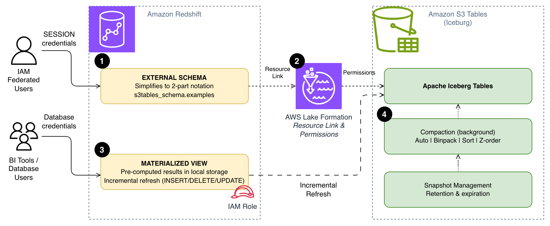
Optimizing S3 Tables queries with external schemas, materialized views, and compaction strategies

Prerequisites

Before you begin, make sure you have:

If you haven’t completed these steps, follow the setup instructions in the first post in this series.

Simplify queries with external schemas

The previous posts in this series used the auto-mounted catalog to query S3 Tables with three-part notation:

SELECT * FROM [email protected];

You can use this syntax, but it can be cumbersome in business intelligence (BI) tools, manually typing queries, and in application code. This syntax also requires the user to use IAM federation. By creating an external schema, you can reference the same tables with a concise two-part notation:

SELECT * FROM s3tables_schema.examples;

To set this up, you create a Lake Formation resource link that maps to your S3 Tables catalog, then create an external schema in Amazon Redshift that points to that resource link. Your setup differs slightly depending on whether your users authenticate through IAM federation or database credentials. While this doesn’t change query performance, it removes a common barrier to adoption by simplifying the reference.

Create a Lake Formation resource link

Both authentication methods require a resource link in Lake Formation that points to your S3 Tables database.

  1. In the Lake Formation console, choose Databases under Data Catalog.
  2. On the Create menu, choose Resource link.
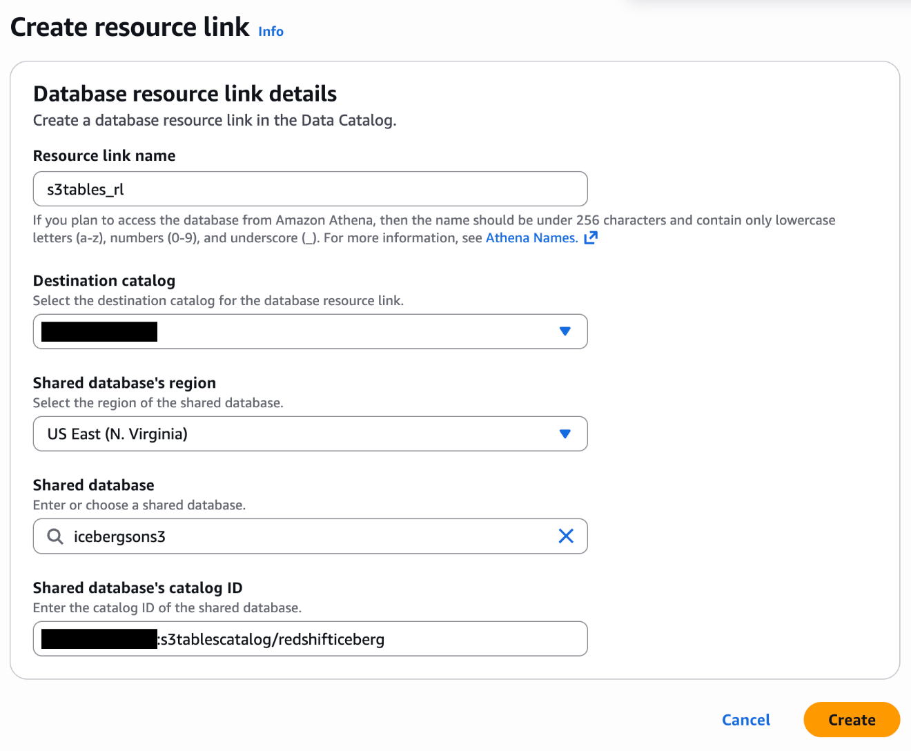
  3. Configure the resource link with the following settings:
    • Resource link name: s3tables_rl
    • Destination Catalog: Your account ID (for example, 111122223333)
    • Shared Database: Your S3 Tables database (for example, icebergsons3)
    • Shared Database’s Catalog ID: Your S3 Table bucket in the format 111122223333:s3tablescatalog/redshifticeberg

Resource link creation in Lake Formation with catalog ID and shared database configured

For more information, see Creating resource links in the Lake Formation documentation.

Option A: External schema for IAM federated users

If your users connect to Amazon Redshift through IAM federation, create the external schema with the SESSION keyword. This passes the federated user’s credentials through to Lake Formation for access control:

CREATE EXTERNAL SCHEMA s3tables_schema
FROM DATA CATALOG
DATABASE 's3tables_rl'
CATALOG_ID '111122223333'
IAM_ROLE 'SESSION'
CATALOG_ROLE 'SESSION';

Lake Formation evaluates your permissions based on your federated user’s IAM role, and sees only the tables and columns their role allows. This is the recommended approach for new deployments because it provides fine-grained access control without additional role management.

Option B: External schema for database users

External applications like Tableau, PowerBI, and custom ETL tools often authenticate with database credentials instead of IAM federation. These users need an IAM role to access S3 Tables on their behalf.

Create an IAM service role to access S3 Tables:

You create a role (for example, S3TableAccessRole) with a trust policy that allows Amazon Redshift to assume it:

{
    "Version": "2012-10-17",
    "Statement": [
        {
            "Effect": "Allow",
            "Principal": {
                "Service": "redshift.amazonaws.com"
            },
            "Action": "sts:AssumeRole"
        }
    ]
}

You then attach the following permission policies to the role:

A policy for Lake Formation data access (substitute your 12-digit AWS Account ID for YOUR_ACCOUNT_ID):

{
    "Version": "2012-10-17",
    "Statement": [
        {
            "Effect": "Allow",
            "Action": "lakeformation:GetDataAccess",
            "Resource": "*",
            "Condition": {
                "StringEquals": {
                    "aws:ResourceAccount": "YOUR_ACCOUNT_ID"
                }
            }
        },
        {
            "Effect": "Deny",
            "Action": "lakeformation:PutDataLakeSettings",
            "Resource": "*",
            "Condition": {
                "StringEquals": {
                    "aws:ResourceAccount": "YOUR_ACCOUNT_ID"
                }
            }
        }
    ]
}

A policy for AWS Glue Data Catalog access (substitute the appropriate AWS Region for REGION_ID and your 12-digit AWS Account ID for YOUR_ACCOUNT_ID):

For production, scope these permissions to your specific resources and AWS Region.

{
    "Version": "2012-10-17",
    "Statement": [
        {
            "Effect": "Allow",
            "Action": [
                "glue:GetTable",
                "glue:GetTables",
                "glue:GetTableVersion",
                "glue:GetTableVersions",
                "glue:GetTags"
            ],
            "Resource": [
                "arn:aws:glue:REGION_ID:YOUR_ACCOUNT_ID:catalog",
                "arn:aws:glue:REGION_ID:YOUR_ACCOUNT_ID:database/*",
                "arn:aws:glue:REGION_ID:YOUR_ACCOUNT_ID:table/*/*"
            ]
        }
    ]
}

Grant Lake Formation permissions to the role:

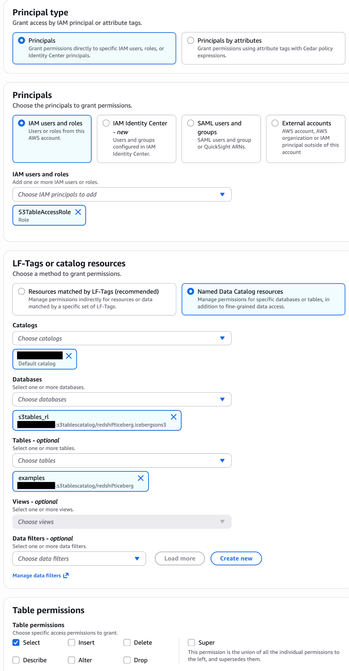
In the Lake Formation console, grant the S3TableAccessRole DESCRIBE access on the database and SELECT access on the tables for your resource link. For detailed steps, see Granting Lake Formation permissions.
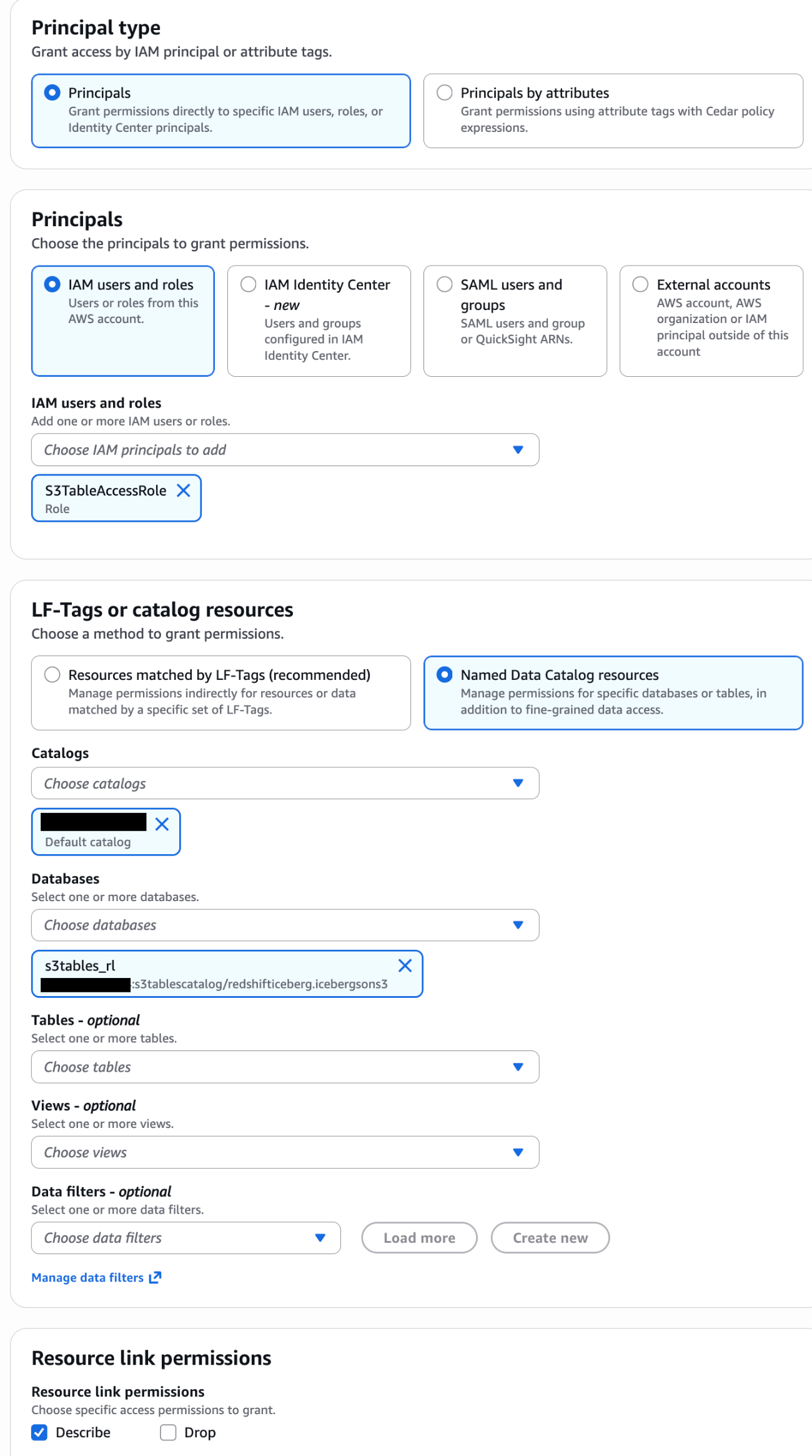
Lake Formation DESCRIBE permission on resource link database

Lake Formation SELECT permission on tables

Associate the role and create the schema:

First, associate the IAM role with your Amazon Redshift cluster or workgroup. For instructions, see Associating IAM roles with Amazon Redshift.

Create the external schema:

CREATE EXTERNAL SCHEMA s3tables_schema
FROM DATA CATALOG
DATABASE 's3tables_rl'
IAM_ROLE 'arn:aws:iam::111122223333:role/S3TableAccessRole';

Then grant access to your database users:

GRANT USAGE ON SCHEMA s3tables_schema TO my_database_user;

Query with two-part notation

With either option, you can now query S3 Tables using the simpler two-part notation:
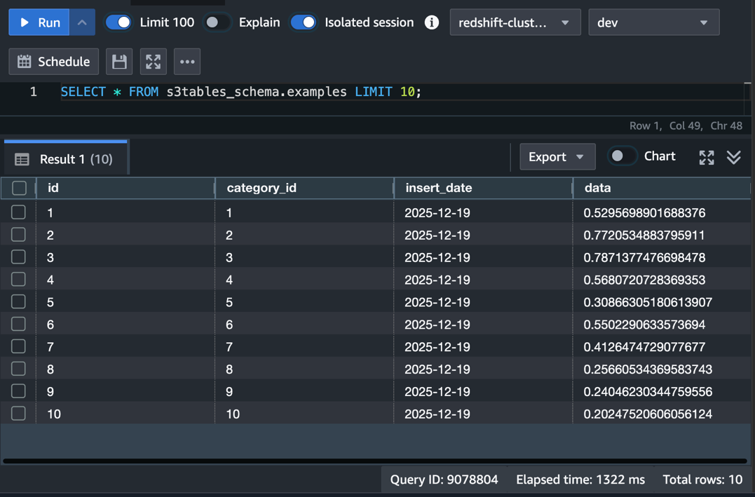
SELECT * FROM s3tables_schema.examples LIMIT 10;

Query results showing two-part notation returning rows from the examples table

You can use this notation in BI tools, JDBC/ODBC connections, and application code and no longer need to know the underlying catalog structure.

Accelerate queries with materialized views

When you repeatedly query S3 Tables, each execution scans the external data from S3. Materialized views store pre-computed results in Amazon Redshift, so subsequent queries read from local storage instead of scanning S3 on every run.

Redshift supports incremental refresh for materialized views on Apache Iceberg tables, including INSERT, DELETE, UPDATE, and table compaction operations. After the initial creation, Amazon Redshift processes only the rows that changed since the last refresh when you run subsequent refreshes, rather than recomputing the full result set. This helps reduce both the time and compute cost of keeping your views current, especially for large tables with frequent changes.

Materialized views have general limitations and considerations when used with external data lake tables. For details, see Materialized views on external data lake tables.

Create a materialized view on S3 Tables

The following example creates a materialized view that joins the examples table in S3 Tables with a local categories table in Amazon Redshift. You can use a materialized view to pre-compute daily record counts and data samples per category:

CREATE MATERIALIZED VIEW mv_daily_category_summary
DISTSTYLE KEY
DISTKEY (category_id)
SORTKEY (insert_date)
AS
SELECT
    c.category_id,
    c.department,
    e.insert_date,
    COUNT(*) AS record_count,
    COUNT(DISTINCT e.id) AS unique_ids
FROM s3tables_schema.examples e
JOIN public.categories c
  ON c.category_id = e.category_id
GROUP BY c.category_id, c.department, e.insert_date;

Query the materialized view directly:

SELECT category_id, department, insert_date, record_count
FROM mv_daily_category_summary
ORDER BY record_count DESC
LIMIT 10;

Your query can now read from local Amazon Redshift storage and typically returns results without scanning S3 Tables:
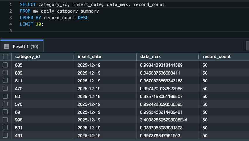
Query results from the materialized view showing category data with record counts

Refresh strategies

You have two options for keeping materialized views current:

Automatic refresh: Set AUTO REFRESH YES in the view definition to have Amazon Redshift automatically refresh the view in the background when it detects changes to the base tables. This is a good fit for dashboards and reports that can tolerate a short delay between data changes and query results. Note that automatic refresh requires Option B (database user) when creating the external schema, and the default is AUTO REFRESH NO.

Manual refresh: Run REFRESH MATERIALIZED VIEW when you need to control the timing:

REFRESH MATERIALIZED VIEW mv_daily_category_summary;

Use manual refresh when you need to coordinate updates with data loading pipelines or when you want to refresh during off-peak hours.

Tune S3 Tables compaction for your query patterns

S3 Tables automatically compacts small Parquet files into larger ones in the background. This compaction reduces the number of read requests your query engine must make, which can improve query performance. By default, compaction targets a file size of 512 MB, configurable between 64 MB and 512 MB. Four compaction strategies are available, and choosing the right one for your query patterns can make a measurable difference.

Compaction strategies

Strategy When to use How it works
Auto You want S3 to decide for you Selects sort compaction for sorted tables, binpack for unsorted tables
Binpack General-purpose workloads, unsorted tables Combines small files into larger files (100 MB+) and applies pending row-level deletes
Sort Queries frequently filter on a single column (e.g., insert_date) Organizes data by the table’s sort-order columns during compaction
Z-order Queries filter on two or more columns together (e.g., insert_date and category_id) Blends multiple column values into a single scalar for sorting

Binpack improves performance by reducing the number of files a query engine reads. Sort compaction goes further. By ordering data within files, it enables query engines to skip entire files based on column min/max metadata during predicate pushdown. This is effective for queries that filter on the sort column, such as date-range filters. Z-order extends this benefit to queries that filter on multiple columns simultaneously, at the cost of slightly less efficient pruning on any single column compared to a pure sort.

To use sort or z-order compaction, you first need to verify that the table is sorted by one (sort) or multiple (z-order) columns:

-- Sort
ALTER TABLE icebergsons3.examples WRITE ORDERED BY insert_date;

-- Z-Order
ALTER TABLE icebergsons3.examples WRITE ORDERED BY insert_date,category_id;

Configure a compaction strategy

To change the compaction strategy for a table, use the PutTableMaintenanceConfiguration API through the AWS Command Line Interface (AWS CLI):

aws s3tables put-table-maintenance-configuration \
    --table-bucket-arn arn:aws:s3tables:us-east-1:111122223333:bucket/redshifticeberg \
    --type icebergCompaction \
    --namespace icebergsons3 \
    --name examples \
    --value '{"status":"enabled","settings":{"icebergCompaction":{"strategy":"sort"}}}'

To adjust the target file size (for example, to 256 MB):

aws s3tables put-table-maintenance-configuration \
    --table-bucket-arn arn:aws:s3tables:us-east-1:111122223333:bucket/redshifticeberg \
    --type icebergCompaction \
    --namespace icebergsons3 \
    --name examples \
    --value '{"status":"enabled","settings":{"icebergCompaction":{"targetFileSizeMB":256}}}'

Similar to the “sort” example, you can specify {"strategy":"z-order"} for z-order compaction.

For more detail on sort and z-order, see Improve Apache Iceberg query performance in Amazon S3 with sort and z-order compaction.

Snapshot management

S3 Tables manage snapshots automatically. By default, it keeps a minimum of 1 snapshot and expires snapshots older than 120 hours (5 days). The snapshot retention is customized by setting minSnapshotsToKeep and maxSnapshotAgeHours. After a snapshot reaches the expiration time you configured in your retention settings, S3 Tables marks objects that only that snapshot references as noncurrent and removes them based on the unreferenced file removal policy.

You can adjust these settings if your workload needs more snapshots for time-travel queries or longer retention:

aws s3tables put-table-maintenance-configuration \
    --table-bucket-arn arn:aws:s3tables:us-east-1:111122223333:bucket/redshifticeberg \
    --namespace icebergsons3 \
    --name examples \
    --type icebergSnapshotManagement \
    --value '{"status":"enabled","settings":{"icebergSnapshotManagement":{"minSnapshotsToKeep":10,"maxSnapshotAgeHours":2500}}}'

Keep in mind that retaining more snapshots increases storage costs. If a materialized view references an expired snapshot, Amazon Redshift falls back to a full recompute on the next refresh. Therefore, snapshot retention can directly affect your materialized view refresh behavior. Balance snapshot retention with your materialized view refresh frequency to avoid unnecessary full recomputes.

For more information, see Maintenance for tables in the Amazon S3 documentation.

Best practices

Choose the right access pattern for your users. Use IAM federation with SESSION credentials for new applications and interactive users. Reserve the IAM role approach for BI tools and extract, transform, and load (ETL) pipelines that can’t integrate with IAM federation directly. Plan to migrate database users to federated access over time.

Match compaction strategy to query patterns. Use sort compaction when your queries filter on a single column (such as date ranges). Use z-order when queries filter on two or more columns together. Stick with the auto default if your query patterns vary or you’re unsure.

Size materialized views for your refresh window. Materialized views that join large external tables with local tables take longer to refresh. If your data changes frequently, keep the materialized view focused on the specific aggregations your dashboards need rather than materializing entire tables.

Coordinate snapshot retention with materialized view refresh. If a materialized view references an expired Iceberg snapshot, Amazon Redshift performs a full recompute instead of an incremental refresh. Set your snapshot retention (maxSnapshotAgeHours) longer than your materialized view refresh interval.

Monitor compaction with AWS CloudTrail. S3 Tables logs compaction operations as CloudTrail management events. Track these to verify that compaction runs on schedule and to identify tables that might benefit from a different strategy.

Balance performance gains against storage costs. Materialized views store pre-computed results in Amazon Redshift, adding to your managed storage. Compaction reduces file counts, but z-order and sort compaction can increase overall storage because of data duplication across sort boundaries. Review your Amazon Redshift managed storage usage and S3 Tables storage metrics periodically to make sure the performance benefits justify the additional storage utilization.

Troubleshooting

Issue Resolution
“Permission denied” when creating the external schema Verify the IAM role has lakeformation:GetDataAccess permission. Confirm you associated the role with your Amazon Redshift cluster or workgroup. Also check that you granted the role access to the resource link database and its tables in Lake Formation.
“Schema not found” or “Database not found” errors Confirm the resource link name in Lake Formation matches the DATABASE value in your CREATE EXTERNAL SCHEMA statement. Verify the catalog ID format uses the pattern account_id:s3tablescatalog/bucket_name.
“Table not found” when querying through the external schema Check that Lake Formation permissions include table-level access, not just database-level. Verify the table exists in the S3 Tables catalog by querying it through the auto-mounted catalog first.
Materialized view refresh falls back to full recompute Check if the referenced Iceberg snapshot has expired. Increase maxSnapshotAgeHours in the snapshot management configuration. Verify that the base table hasn’t exceeded 4 million position deletes in a single data file. Compaction resolves this.
Queries on S3 Tables are slow after data loading Compaction runs on an automated schedule and may not have processed recent writes yet. Check CloudTrail for the latest compaction event. Verify the compaction strategy matches your query patterns. Switch from binpack to sort if you filter on specific columns.

Cleaning up

To avoid ongoing costs, remove the resources you created in this walkthrough:

-- Drop materialized views
DROP MATERIALIZED VIEW IF EXISTS mv_daily_category_summary;

-- Drop external schemas
DROP SCHEMA IF EXISTS s3tables_schema;

Also remove:

  • The IAM role (S3TableAccessRole) and its attached policies, if you created one for database users.
  • The Lake Formation resource link and associated permissions.
  • The S3 table bucket, if you no longer need the data.

Conclusion

In this post, we showed how to optimize S3 Tables queries from Amazon Redshift using three approaches: external schemas that simplify query syntax from three-part to two-part notation, making it easier for BI tools and end users to work with S3 Tables. We also covered materialized views for pre-computed analytical results that reduce repeated S3 scans, and S3 Tables compaction strategies tuned to your query patterns for more efficient file access.

For new applications, design your access layer with IAM federation and external schemas from the start. Use materialized views to accelerate repeated analytical queries that join S3 Tables with local Amazon Redshift data. Match your compaction strategy to how your team queries the data. Use sort compaction for date-range filters and z-order when queries filter on multiple columns at once. Furthermore, the same S3 tables you optimize here are also accessible from Amazon Athena, Amazon EMR, and third-party engines.

To learn more, see the Amazon S3 Tables documentation, Materialized views in Amazon Redshift, and S3 Tables maintenance. We welcome your feedback in the comments.
About the authors

Tom Romano

Tom Romano

Tom Romano is a Senior Solutions Architect for AWS World Wide Public Sector based in Tampa, FL. He works with GovTech customers to build solutions using serverless architectures, generative AI, and modern data and DevOps practices. In his free time, Tom flies remote control model airplanes and enjoys vacationing with his family around Florida and the Caribbean.

Satesh Sonti

Satesh Sonti

Satesh Sonti is a Principal Analytics Specialist Solutions Architect based out of Atlanta, specializing in building enterprise data platforms, data warehousing, and analytics solutions. He has over 20 years of experience in building data assets and leading complex data platform programs for banking and insurance clients across the globe.

Empower your Jira data in a data lake with Amazon AppFlow and AWS Glue

Post Syndicated from Tom Romano original https://aws.amazon.com/blogs/big-data/empower-your-jira-data-in-a-data-lake-with-amazon-appflow-and-aws-glue/

In the world of software engineering and development, organizations use project management tools like Atlassian Jira Cloud. Managing projects with Jira leads to rich datasets, which can provide historical and predictive insights about project and development efforts.

Although Jira Cloud provides reporting capability, loading this data into a data lake will facilitate enrichment with other business data, as well as support the use of business intelligence (BI) tools and artificial intelligence (AI) and machine learning (ML) applications. Companies often take a data lake approach to their analytics, bringing data from many different systems into one place to simplify how the analytics are done.

This post shows you how to use Amazon AppFlow and AWS Glue to create a fully automated data ingestion pipeline that will synchronize your Jira data into your data lake. Amazon AppFlow provides software as a service (SaaS) integration with Jira Cloud to load the data into your AWS account. AWS Glue is a serverless data discovery, load, and transformation service that will prepare data for consumption in BI and AI/ML activities. Additionally, this post strives to achieve a low-code and serverless solution for operational efficiency and cost optimization, and the solution supports incremental loading for cost optimization.

Solution overview

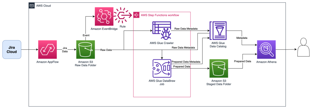
This solution uses Amazon AppFlow to retrieve data from the Jira Cloud. The data is synchronized to an Amazon Simple Storage Service (Amazon S3) bucket using an initial full download and subsequent incremental downloads of changes. When new data arrives in the S3 bucket, an AWS Step Functions workflow is triggered that orchestrates extract, transform, and load (ETL) activities using AWS Glue crawlers and AWS Glue DataBrew. The data is then available in the AWS Glue Data Catalog and can be queried by services such as Amazon Athena, Amazon QuickSight, and Amazon Redshift Spectrum. The solution is completely automated and serverless, resulting in low operational overhead. When this setup is complete, your Jira data will be automatically ingested and kept up to date in your data lake!

The following diagram illustrates the solution architecture.

The Jira Appflow Architecture is shown. The Jira Cloud data is retrieved by Amazon AppFlow and is stored in Amazon S3. This triggers an Amazon EventBridge event that runs an AWS Step Functions workflow. The workflow uses AWS Glue to catalog and transform the data, The data is then queried with QuickSight.

The Step Functions workflow orchestrates the following ETL activities, resulting in two tables:

  • An AWS Glue crawler collects all downloads into a single AWS Glue table named jira_raw. This table is comprised of a mix of full and incremental downloads from Jira, with many versions of the same records representing changes over time.
  • A DataBrew job prepares the data for reporting by unpacking key-value pairs in the fields, as well as removing depreciated records as they are updated in subsequent change data captures. This reporting-ready data will available in an AWS Glue table named jira_data.

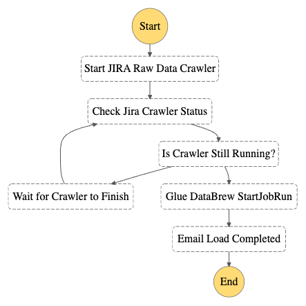
The following figure shows the Step Functions workflow.

A diagram represents the AWS Step Functions workflow. It contains the steps to run an AWS Crawler, wait for it's completion, and then run a AWS Glue DataBrew data transformation job.

Prerequisites

This solution requires the following:

  • Administrative access to your Jira Cloud instance, and an associated Jira Cloud developer account.
  • An AWS account and a login with access to the AWS Management Console. Your login will need AWS Identity and Access Management (IAM) permissions to create and access the resources in your AWS account.
  • Basic knowledge of AWS and working knowledge of Jira administration.

Configure the Jira Instance

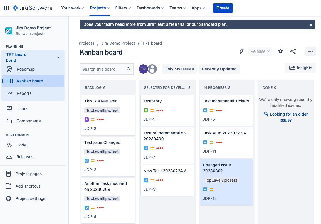
After logging in to your Jira Cloud instance, you establish a Jira project with associated epics and issues to download into a data lake. If you’re starting with a new Jira instance, it helps to have at least one project with a sampling of epics and issues for the initial data download, because it allows you to create an initial dataset without errors or missing fields. Note that you may have multiple projects as well.

An image show a Jira Cloud example, with several issues arranged in a Kansan board.

After you have established your Jira project and populated it with epics and issues, ensure you also have access to the Jira developer portal. In later steps, you use this developer portal to establish authentication and permissions for the Amazon AppFlow connection.

Provision resources with AWS CloudFormation

For the initial setup, you launch an AWS CloudFormation stack to create an S3 bucket to store data, IAM roles for data access, and the AWS Glue crawler and Data Catalog components. Complete the following steps:

  1. Sign in to your AWS account.
  2. Click Launch Stack:
  3. For Stack name, enter a name for the stack (the default is aws-blog-jira-datalake-with-AppFlow).
  4. For GlueDatabaseName, enter a unique name for the Data Catalog database to hold the Jira data table metadata (the default is jiralake).
  5. For InitialRunFlag, choose Setup. This mode will scan all data and disable the change data capture (CDC) features of the stack. (Because this is the initial load, the stack needs an initial data load before you configure CDC in later steps.)
  6. Under Capabilities and transforms, select the acknowledgement check boxes to allow IAM resources to be created within your AWS account.
  7. Review the parameters and choose Create stack to deploy the CloudFormation stack. This process will take around 5–10 minutes to complete.
    An image depicts the Amazon CloudFormation configuration steps, including setting a stack name, setting parameters to "jiralake" and "Setup" mode, and checking all IAM capabilities requested.
  8. After the stack is deployed, review the Outputs tab for the stack and collect the following values to use when you set up Amazon AppFlow:
    • Amazon AppFlow destination bucket (o01AppFlowBucket)
    • Amazon AppFlow destination bucket path (o02AppFlowPath)
    • Role for Amazon AppFlow Jira connector (o03AppFlowRole)
      An image demonstrating the Amazon Cloudformation "Outputs" tab, highlighting the values to add to the Amazon AppFlow configuration.

Configure Jira Cloud

Next, you configure your Jira Cloud instance for access by Amazon AppFlow. For full instructions, refer to Jira Cloud connector for Amazon AppFlow. The following steps summarize these instructions and discuss the specific configuration to enable OAuth in the Jira Cloud:

  1. Open the Jira developer portal.
  2. Create the OAuth 2 integration from the developer application console by choosing Create an OAuth 2.0 Integration. This will provide a login mechanism for AppFlow.
  3. Enable fine-grained permissions. See Recommended scopes for the permission settings to grant AppFlow appropriate access to your Jira instance.
  4. Add the following permission scopes to your OAuth app:
    1. manage:jira-configuration
    2. read:field-configuration:jira
  5. Under Authorization, set the Call Back URL to return to Amazon AppFlow with the URL https://us-east-1.console.aws.amazon.com/AppFlow/oauth.
  6. Under Settings, note the client ID and secret to use in later steps to set up authentication from Amazon AppFlow.

Create the Amazon AppFlow Jira Cloud connection

In this step, you configure Amazon AppFlow to run a one-time full data fetch of all your data, establishing the initial data lake:

  1. On the Amazon AppFlow console, choose Connectors in the navigation pane.
  2. Search for the Jira Cloud connector.
  3. Choose Create flow on the connector tile to create the connection to your Jira instance.
    An image of Amazon AppFlor, showing the search for the "Jira Cloud" connector.
  4. For Flow name, enter a name for the flow (for example, JiraLakeFlow).
  5. Leave the Data encryption setting as the default.
  6. Choose Next.
    The Amazon AppFlow Jira connector configuration, showing the Flow name set to "JiraLakeFlow" and clicking the "next" button.
  7. For Source name, keep the default of Jira Cloud.
  8. Choose Create new connection under Jira Cloud connection.
  9. In the Connect to Jira Cloud section, enter the values for Client ID, Client secret, and Jira Cloud Site that you collected earlier. This provides the authentication from AppFlow to Jira Cloud.
  10. For Connection Name, enter a connection name (for example, JiraLakeCloudConnection).
  11. Choose Connect. You will be prompted to allow your OAuth app to access your Atlassian account to verify authentication.
    An image of the Amazon AppFlow conflagration, reflecting the completion of the prior steps.
  12. In the Authorize App window that pops up, choose Accept.
  13. With the connection created, return to the Configure flow section on the Amazon AppFlow console.
  14. For API version, choose V2 to use the latest Jira query API.
  15. For Jira Cloud object, choose Issue to query and download all issues and associated details.
    An image of the Amazon AppFlow configuration, reflecting the completion of the prior steps.
  16. For Destination Name in the Destination Details section, choose Amazon S3.
  17. For Bucket details, choose the S3 bucket name that matches the Amazon AppFlow destination bucket value that you collected from the outputs of the CloudFormation stack.
  18. Enter the Amazon AppFlow destination bucket path to complete the full S3 path. This will send the Jira data to the S3 bucket created by the CloudFormation script.
  19. Leave Catalog your data in the AWS Glue Data Catalog unselected. The CloudFormation script uses an AWS Glue crawler to update the Data Catalog in a different manner, grouping all the downloads into a common table, so we disable the update here.
  20. For File format settings, select Parquet format and select Preserve source data types in Parquet output. Parquet is a columnar format to optimize subsequent querying.
  21. Select Add a timestamp to the file name for Filename preference. This will allow you to easily find data files downloaded at a specific date and time.
    An image of the Amazon AppFlow configuration, reflecting the completion of the prior steps.
  22. For now, select Run on Demand for the Flow trigger to run the full load flow manually. You will schedule downloads in a later step when implementing CDC.
  23. Choose Next.
    An image of the Amazon AppFlow Flow Trigger configuration, reflecting the completion of the prior steps.
  24. On the Map data fields page, select Manually map fields.
  25. For Source to destination field mapping, choose the drop-down box under Source field name and select Map all fields directly. This will bring down all fields as they are received, because we will instead implement data preparation in later steps.
    An image of the Amazon AppFlow configuration, reflecting the completion of steps 24 & 25.
  26. Under Partition and aggregation settings, you can set up the partitions in a way that works for your use case. For this example, we use a daily partition, so select Date and time and choose Daily.
  27. For Aggregation settings, leave it as the default of Don’t aggregate.
  28. Choose Next.
    An image of the Amazon AppFlow configuration, reflecting the completion of steps 26-28.
  29. On the Add filters page, you can create filters to only download specific data. For this example, you download all the data, so choose Next.
  30. Review and choose Create flow.
  31. When the flow is created, choose Run flow to start the initial data seeding. After some time, you should receive a banner indicating the run finished successfully.
    An image of the Amazon AppFlow configuration, reflecting the completion of step 31.

Review seed data

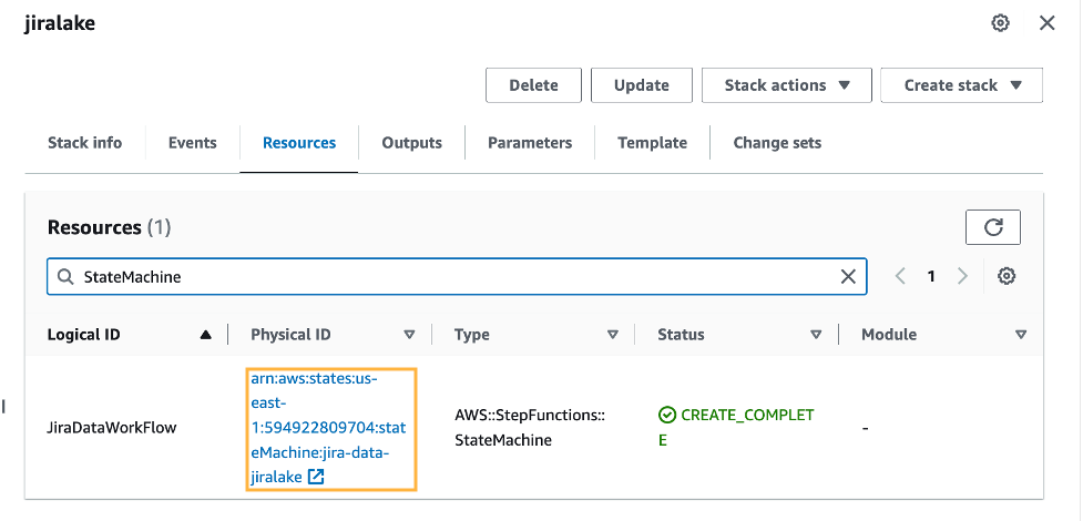
At this stage in the process, you now have data in your S3 environment. When new data files are created in the S3 bucket, it will automatically run an AWS Glue crawler to catalog the new data. You can see if it’s complete by reviewing the Step Functions state machine for a Succeeded run status. There is a link to the state machine on the CloudFormation stack’s Resources tab, which will redirect you to the Step Functions state machine.

A image showing the CloudFormation resources tab of the stack, with a link to the AWS Step Functions workflow.

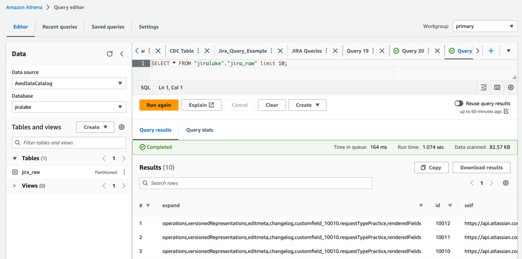
When the state machine is complete, it’s time to review the raw Jira data with Athena. The database is as you specified in the CloudFormation stack (jiralake by default), and the table name is jira_raw. If you kept the default AWS Glue database name of jiralake, the Athena SQL is as follows:

SELECT * FROM "jiralake"."jira_raw" limit 10;

If you explore the data, you’ll notice that most of the data you would want to work with is actually packed into a column called fields. This means the data is not available as columns in your Athena queries, making it harder to select, filter, and sort individual fields within an Athena SQL query. This will be addressed in the next steps.

An image demonstrating the Amazon Athena query SELECT * FROM "jiralake"."jira_raw" limit 10;

Set up CDC and unpack the fields columns

To add the ongoing CDC and reformat the data for analytics, we introduce a DataBrew job to transform the data and filter to the most recent version of each record as changes come in. You can do this by updating the CloudFormation stack with a flag that includes the CDC and data transformation steps.

  1. On the AWS CloudFormation console, return to the stack.
  2. Choose Update.
  3. Select Use current template and choose Next.
    An image showing Amazon CloudFormation, with steps 1-3 complete.
  4. For SetupOrCDC, choose CDC, then choose Next. This will enable both the CDC steps and the data transformation steps for the Jira data.
    An image showing Amazon CloudFormation, with step 4 complete.
  5. Continue choosing Next until you reach the Review section.
  6. Select I acknowledge that AWS CloudFormation might create IAM resources, then choose Submit.
    An image showing Amazon CloudFormation, with step 5-6 complete.
  7. Return to the Amazon AppFlow console and open your flow.
  8. On the Actions menu, choose Edit flow. We will now edit the flow trigger to run an incremental load on a periodic basis.
  9. Select Run flow on schedule.
  10. Configure the desired repeats, as well as start time and date. For this example, we choose Daily for Repeats and enter 1 for the number of days you’ll have the flow trigger. For Starting at, enter 01:00.
  11. Select Incremental transfer for Transfer mode.
  12. Choose Updated on the drop-down menu so that changes will be captured based on when the records were updated.
  13. Choose Save. With these settings in our example, the run will happen nightly at 1:00 AM.
    An image showing the Flow Trigger, with incremental transfer selected.

Review the analytics data

When the next incremental load occurs that results in new data, the Step Functions workflow will start the DataBrew job and populate a new staged analytical data table named jira_data in your Data Catalog database. If you don’t want to wait, you can trigger the Step Functions workflow manually.

The DataBrew job performs data transformation and filtering tasks. The job unpacks the key-values from the Jira JSON data and the raw Jira data, resulting in a tabular data schema that facilitates use with BI and AI/ML tools. As Jira items are changed, the changed item’s data is resent, resulting in multiple versions of an item in the raw data feed. The DataBrew job filters the raw data feed so that the resulting data table only contains the most recent version of each item. You could enhance this DataBrew job to further customize the data for your needs, such as renaming the generic Jira custom field names to reflect their business meaning.

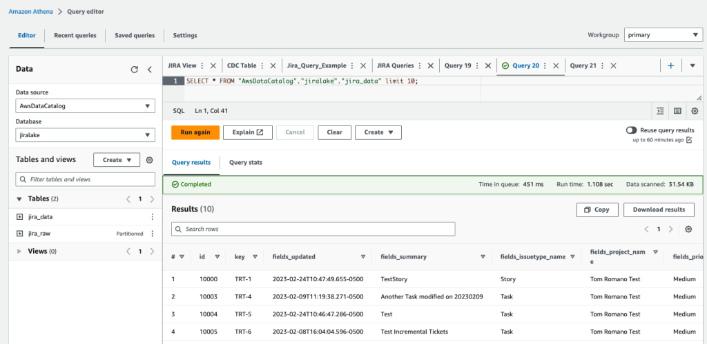
When the Step Functions workflow is complete, we can query the data in Athena again using the following query:

SELECT * FROM "jiralake"."jira_data" limit 10;

You can see that in our transformed jira_data table, the nested JSON fields are broken out into their own columns for each field. You will also notice that we’ve filtered out obsolete records that have been superseded by more recent record updates in later data loads so the data is fresh. If you want to rename custom fields, remove columns, or restructure what comes out of the nested JSON, you can modify the DataBrew recipe to accomplish this. At this point, the data is ready to be used by your analytics tools, such as Amazon QuickSight.

An image demonstrating the Amazon Athena query SELECT * FROM "jiralake"."jira_data" limit 10;

Clean up

If you would like to discontinue this solution, you can remove it with the following steps:

  1. On the Amazon AppFlow console, deactivate the flow for Jira, and optionally delete it.
  2. On the Amazon S3 console, select the S3 bucket for the stack, and empty the bucket to delete the existing data.
  3. On the AWS CloudFormation console, delete the CloudFormation stack that you deployed.

Conclusion

In this post, we created a serverless incremental data load process for Jira that will synchronize data while handling custom fields using Amazon AppFlow, AWS Glue, and Step Functions. The approach uses Amazon AppFlow to incrementally load the data into Amazon S3. We then use AWS Glue and Step Functions to manage the extraction of the Jira custom fields and load them in a format to be queried by analytics services such as Athena, QuickSight, or Redshift Spectrum, or AI/ML services like Amazon SageMaker.

To learn more about AWS Glue and DataBrew, refer to Getting started with AWS Glue DataBrew. With DataBrew, you can take the sample data transformation in this project and customize the output to meet your specific needs. This could include renaming columns, creating additional fields, and more.

To learn more about Amazon AppFlow, refer to Getting started with Amazon AppFlow. Note that Amazon AppFlow supports integrations with many SaaS applications in addition to the Jira Cloud.

To learn more about orchestrating flows with Step Functions, see Create a Serverless Workflow with AWS Step Functions and AWS Lambda. The workflow could be enhanced to load the data into a data warehouse, such as Amazon Redshift, or trigger a refresh of a QuickSight dataset for analytics and reporting.

In future posts, we will cover how to unnest parent-child relationships within the Jira data using Athena and how to visualize the data using QuickSight.


About the Authors

Tom Romano is a Sr. Solutions Architect for AWS World Wide Public Sector from Tampa, FL, and assists GovTech and EdTech customers as they create new solutions that are cloud native, event driven, and serverless. He is an enthusiastic Python programmer for both application development and data analytics, and is an Analytics Specialist. In his free time, Tom flies remote control model airplanes and enjoys vacationing with his family around Florida and the Caribbean.

Shane Thompson is a Sr. Solutions Architect based out of San Luis Obispo, California, working with AWS Startups. He works with customers who use AI/ML in their business model and is passionate about democratizing AI/ML so that all customers can benefit from it. In his free time, Shane loves to spend time with his family and travel around the world.