Tag Archives: AWS Glue DataBrew

Detect, mask, and redact PII data using AWS Glue before loading into Amazon OpenSearch Service

Post Syndicated from Michael Hamilton original https://aws.amazon.com/blogs/big-data/detect-mask-and-redact-pii-data-using-aws-glue-before-loading-into-amazon-opensearch-service/

Many organizations, small and large, are working to migrate and modernize their analytics workloads on Amazon Web Services (AWS). There are many reasons for customers to migrate to AWS, but one of the main reasons is the ability to use fully managed services rather than spending time maintaining infrastructure, patching, monitoring, backups, and more. Leadership and development teams can spend more time optimizing current solutions and even experimenting with new use cases, rather than maintaining the current infrastructure.

With the ability to move fast on AWS, you also need to be responsible with the data you’re receiving and processing as you continue to scale. These responsibilities include being compliant with data privacy laws and regulations and not storing or exposing sensitive data like personally identifiable information (PII) or protected health information (PHI) from upstream sources.

In this post, we walk through a high-level architecture and a specific use case that demonstrates how you can continue to scale your organization’s data platform without needing to spend large amounts of development time to address data privacy concerns. We use AWS Glue to detect, mask, and redact PII data before loading it into Amazon OpenSearch Service.

Solution overview

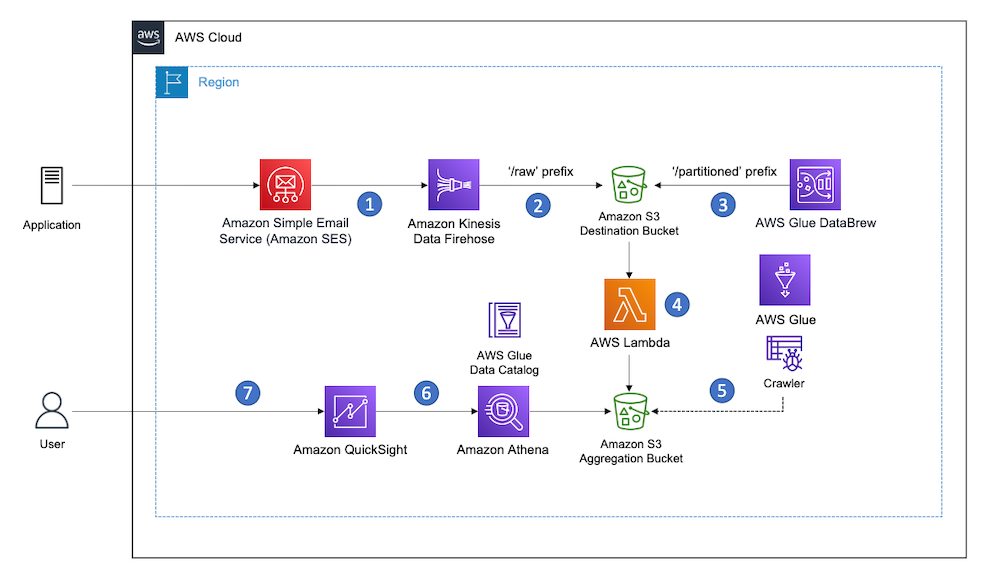
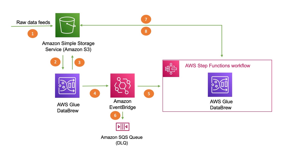
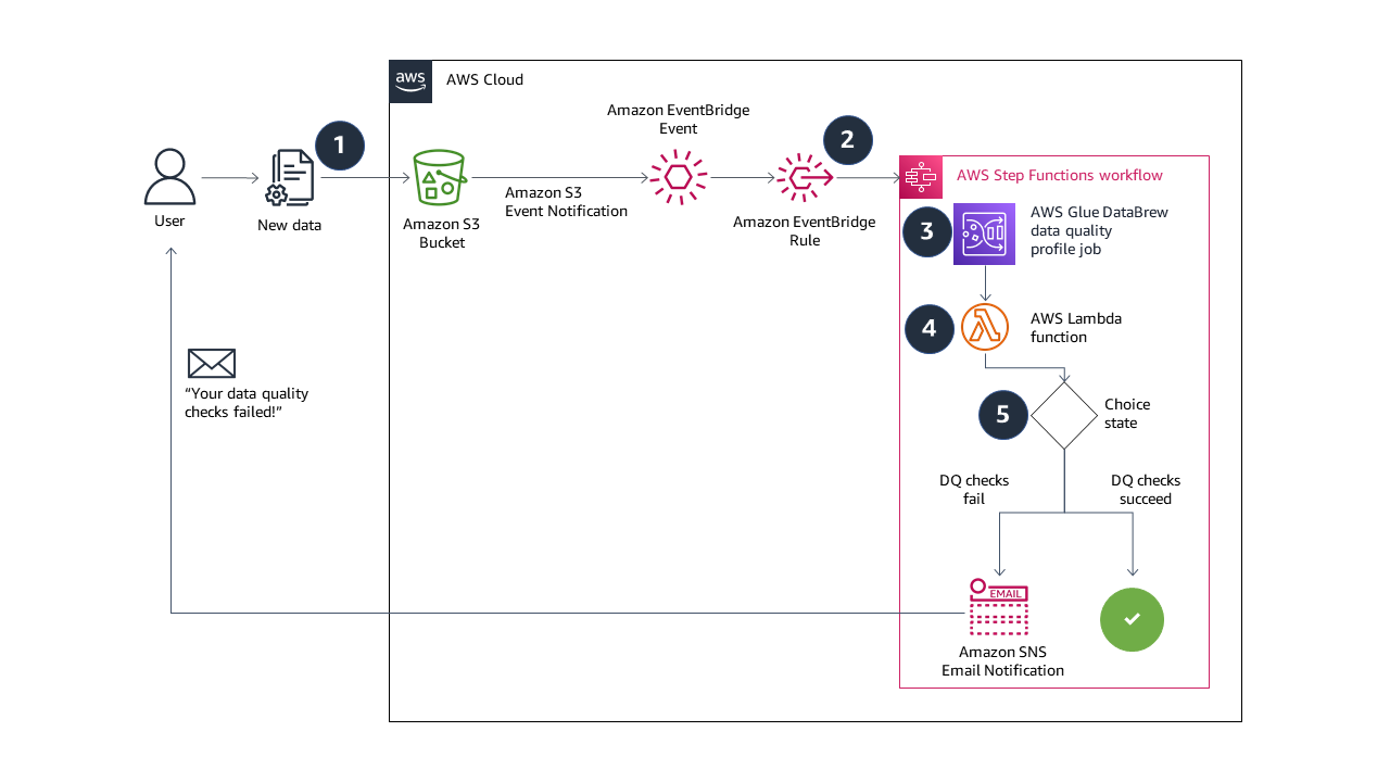
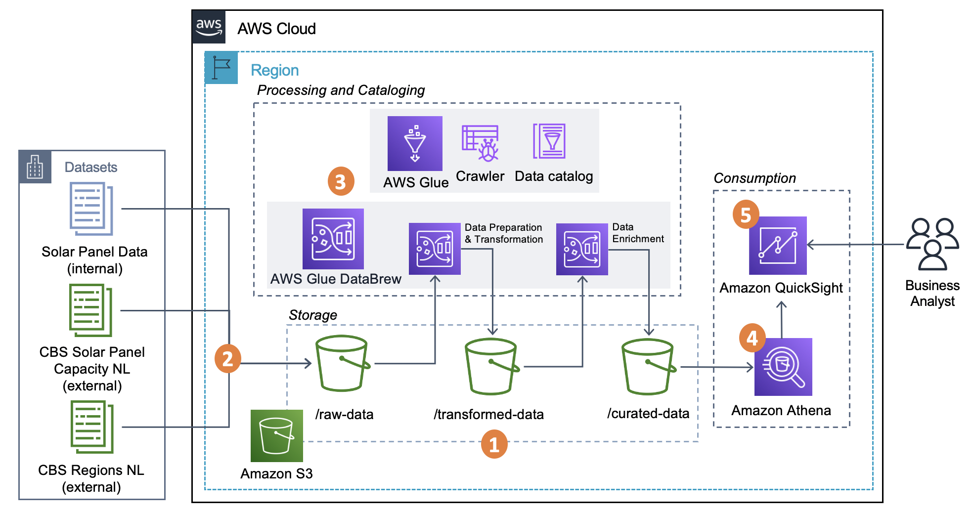
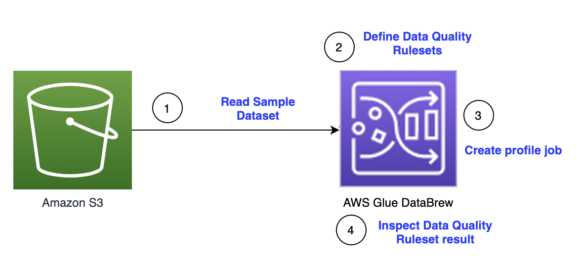
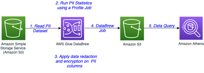
The following diagram illustrates the high-level solution architecture. We have defined all layers and components of our design in line with the AWS Well-Architected Framework Data Analytics Lens.

os_glue_architecture

The architecture is comprised of a number of components:

Source data

Data may be coming from many tens to hundreds of sources, including databases, file transfers, logs, software as a service (SaaS) applications, and more. Organizations may not always have control over what data comes through these channels and into their downstream storage and applications.

Ingestion: Data lake batch, micro-batch, and streaming

Many organizations land their source data into their data lake in various ways, including batch, micro-batch, and streaming jobs. For example, Amazon EMR, AWS Glue, and AWS Database Migration Service (AWS DMS) can all be used to perform batch and or streaming operations that sink to a data lake on Amazon Simple Storage Service (Amazon S3). Amazon AppFlow can be used to transfer data from different SaaS applications to a data lake. AWS DataSync and AWS Transfer Family can help with moving files to and from a data lake over a number of different protocols. Amazon Kinesis and Amazon MSK also have capabilities to stream data directly to a data lake on Amazon S3.

S3 data lake

Using Amazon S3 for your data lake is in line with the modern data strategy. It provides low-cost storage without sacrificing performance, reliability, or availability. With this approach, you can bring compute to your data as needed and only pay for capacity it needs to run.

In this architecture, raw data can come from a variety of sources (internal and external), which may contain sensitive data.

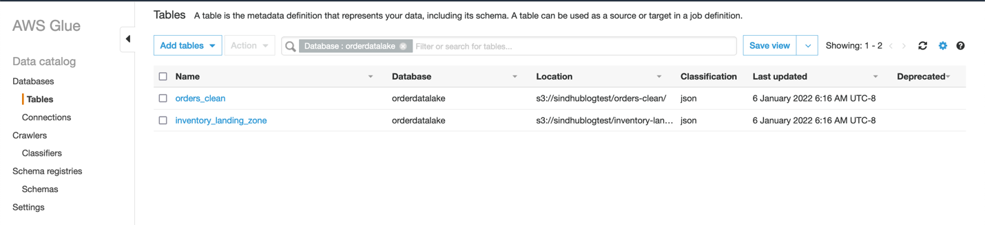
Using AWS Glue crawlers, we can discover and catalog the data, which will build the table schemas for us, and ultimately make it straightforward to use AWS Glue ETL with the PII transform to detect and mask or and redact any sensitive data that may have landed in the data lake.

Business context and datasets

To demonstrate the value of our approach, let’s imagine you’re part of a data engineering team for a financial services organization. Your requirements are to detect and mask sensitive data as it is ingested into your organization’s cloud environment. The data will be consumed by downstream analytical processes. In the future, your users will be able to safely search historical payment transactions based on data streams collected from internal banking systems. Search results from operation teams, customers, and interfacing applications must be masked in sensitive fields.

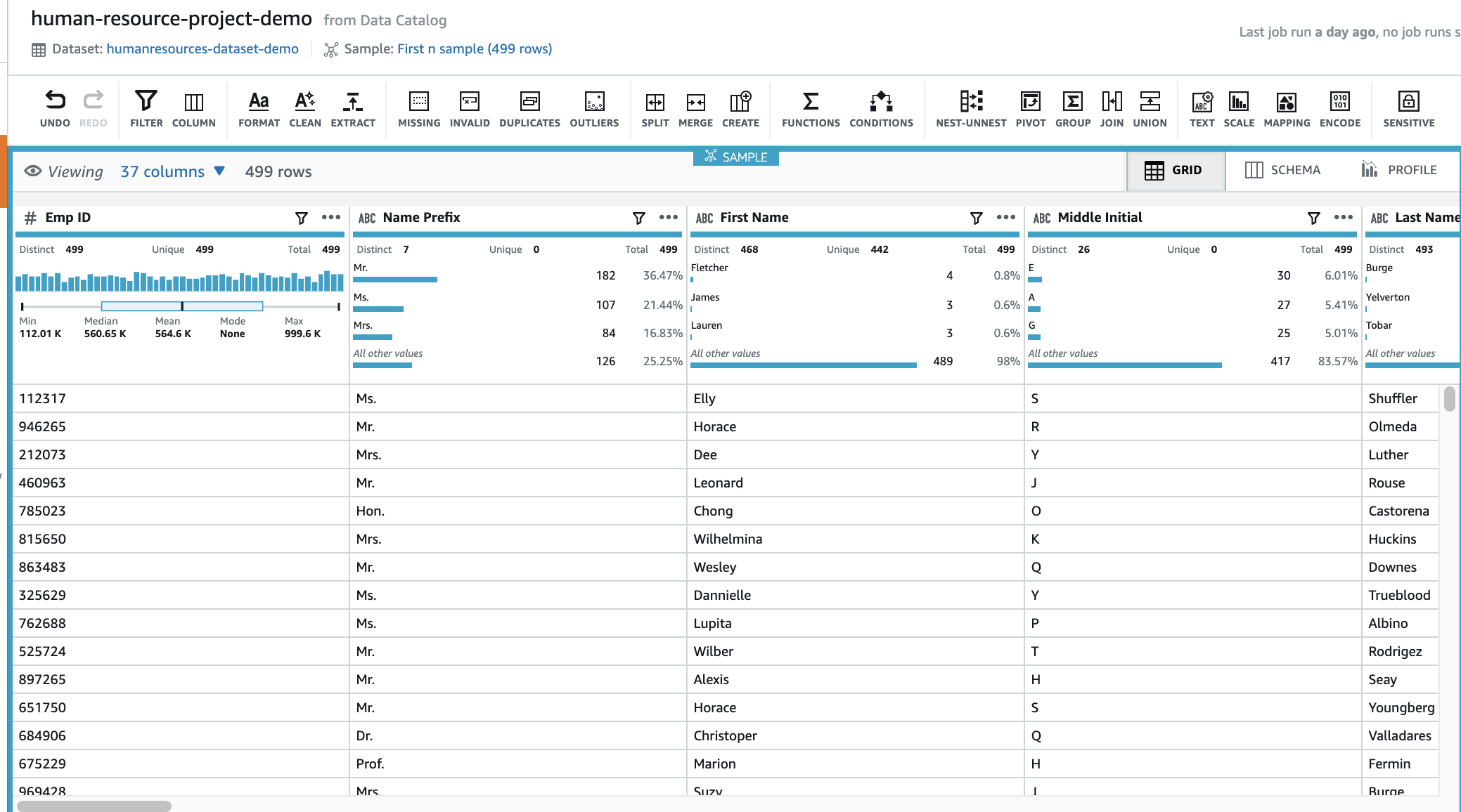
The following table shows the data structure used for the solution. For clarity, we have mapped raw to curated column names. You’ll notice that multiple fields within this schema are considered sensitive data, such as first name, last name, Social Security number (SSN), address, credit card number, phone number, email, and IPv4 address.

Raw Column Name Curated Column Name Type
c0 first_name string
c1 last_name string
c2 ssn string
c3 address string
c4 postcode string
c5 country string
c6 purchase_site string
c7 credit_card_number string
c8 credit_card_provider string
c9 currency string
c10 purchase_value integer
c11 transaction_date date
c12 phone_number string
c13 email string
c14 ipv4 string

Use case: PII batch detection before loading to OpenSearch Service

Customers who implement the following architecture have built their data lake on Amazon S3 to run different types of analytics at scale. This solution is suitable for customers who don’t require real-time ingestion to OpenSearch Service and plan to use data integration tools that run on a schedule or are triggered through events.

batch_architecture

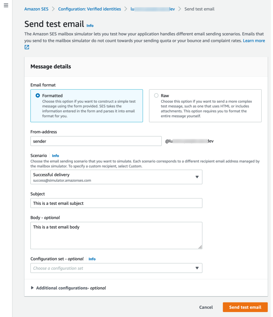
Before data records land on Amazon S3, we implement an ingestion layer to bring all data streams reliably and securely to the data lake. Kinesis Data Streams is deployed as an ingestion layer for accelerated intake of structured and semi-structured data streams. Examples of these are relational database changes, applications, system logs, or clickstreams. For change data capture (CDC) use cases, you can use Kinesis Data Streams as a target for AWS DMS. Applications or systems generating streams containing sensitive data are sent to the Kinesis data stream via one of the three supported methods: the Amazon Kinesis Agent, the AWS SDK for Java, or the Kinesis Producer Library. As a last step, Amazon Kinesis Data Firehose helps us reliably load near-real-time batches of data into our S3 data lake destination.

The following screenshot shows how data flows through Kinesis Data Streams via the Data Viewer and retrieves sample data that lands on the raw S3 prefix. For this architecture, we followed the data lifecycle for S3 prefixes as recommended in Data lake foundation.

kinesis raw data

As you can see from the details of the first record in the following screenshot, the JSON payload follows the same schema as in the previous section. You can see the unredacted data flowing into the Kinesis data stream, which will be obfuscated later in subsequent stages.

raw_json

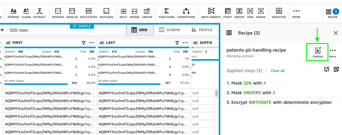
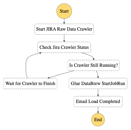
After the data is collected and ingested into Kinesis Data Streams and delivered to the S3 bucket using Kinesis Data Firehose, the processing layer of the architecture takes over. We use the AWS Glue PII transform to automate detection and masking of sensitive data in our pipeline. As shown in the following workflow diagram, we took a no-code, visual ETL approach to implement our transformation job in AWS Glue Studio.

glue studio nodes

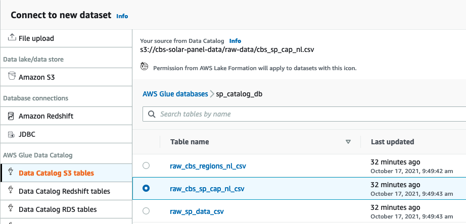
First, we access the source Data Catalog table raw from the pii_data_db database. The table has the schema structure presented in the previous section. To keep track of the raw processed data, we used job bookmarks.

glue catalog

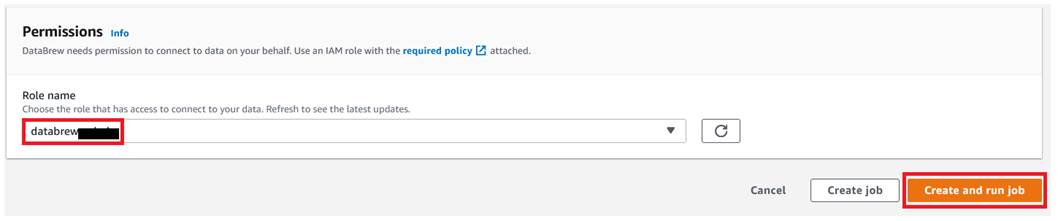
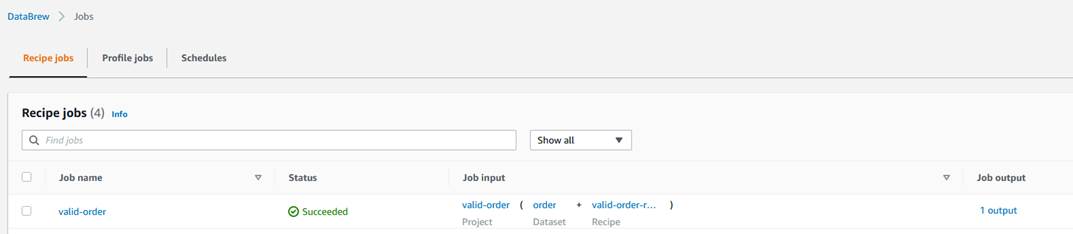
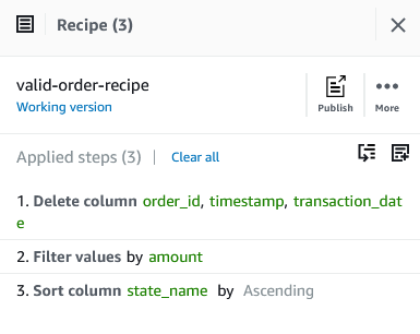
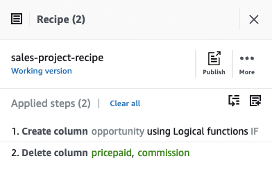
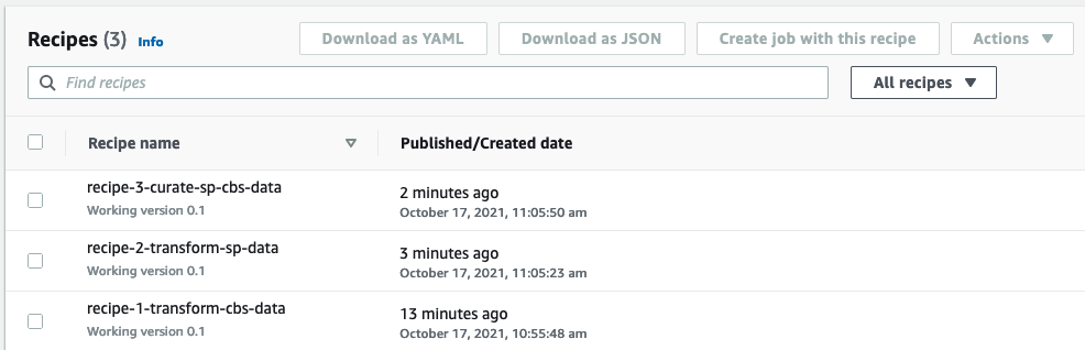
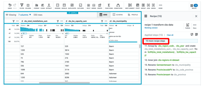
We use the AWS Glue DataBrew recipes in the AWS Glue Studio visual ETL job to transform two date attributes to be compatible with OpenSearch expected formats. This allows us to have a full no-code experience.

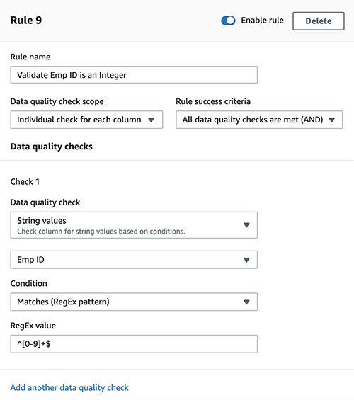
We use the Detect PII action to identify sensitive columns. We let AWS Glue determine this based on selected patterns, detection threshold, and sample portion of rows from the dataset. In our example, we used patterns that apply specifically to the United States (such as SSNs) and may not detect sensitive data from other countries. You may look for available categories and locations applicable to your use case or use regular expressions (regex) in AWS Glue to create detection entities for sensitive data from other countries.

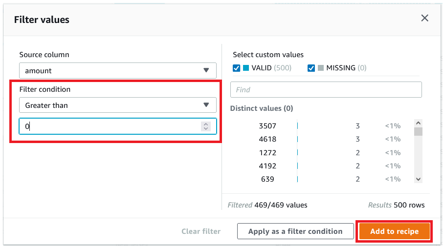
It’s important to select the correct sampling method that AWS Glue offers. In this example, it’s known that the data coming in from the stream has sensitive data in every row, so it’s not necessary to sample 100% of the rows in the dataset. If you have a requirement where no sensitive data is allowed to downstream sources, consider sampling 100% of the data for the patterns you chose, or scan the entire dataset and act on each individual cell to ensure all sensitive data is detected. The benefit you get from sampling is reduced costs because you don’t have to scan as much data.

PII Options

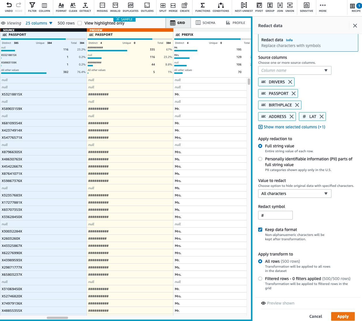
The Detect PII action allows you to select a default string when masking sensitive data. In our example, we use the string **********.

selected_options

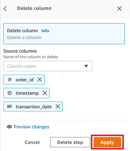
We use the apply mapping operation to rename and remove unnecessary columns such as ingestion_year, ingestion_month, and ingestion_day. This step also allows us to change the data type of one of the columns (purchase_value) from string to integer.

schema

From this point on, the job splits into two output destinations: OpenSearch Service and Amazon S3.

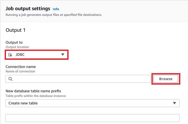
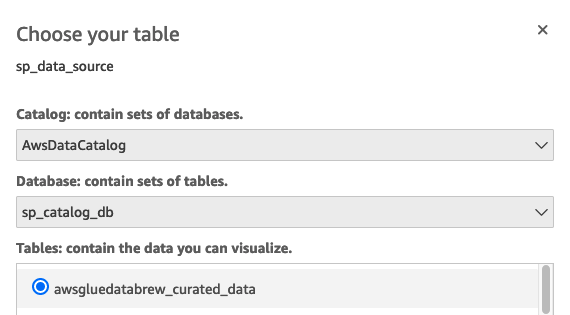
Our provisioned OpenSearch Service cluster is connected via the OpenSearch built-in connector for Glue. We specify the OpenSearch Index we’d like to write to and the connector handles the credentials, domain and port. In the screen shot below, we write to the specified index index_os_pii.

opensearch config

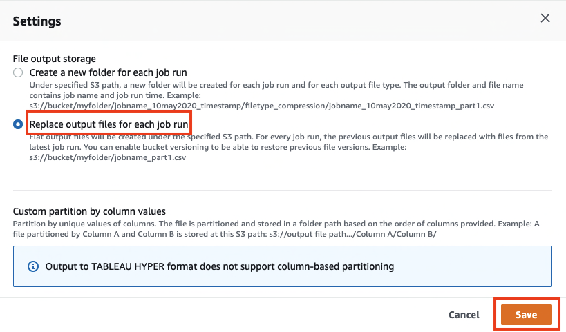
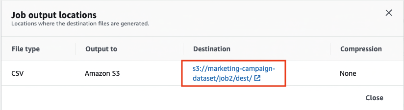
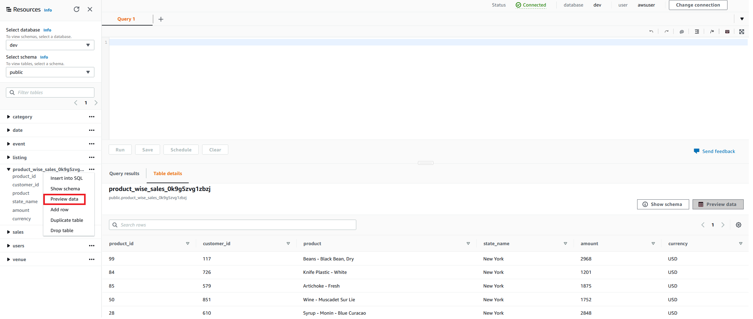
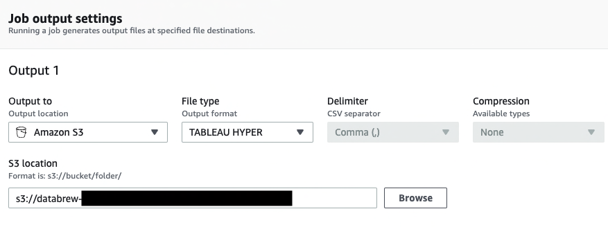
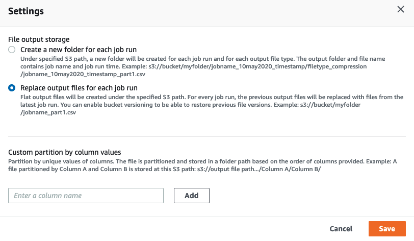
We store the masked dataset in the curated S3 prefix. There, we have data normalized to a specific use case and safe consumption by data scientists or for ad hoc reporting needs.

opensearch target s3 folder

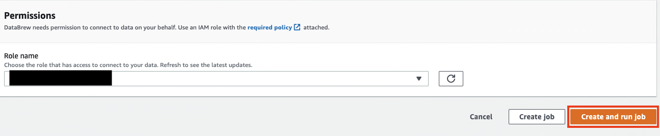
For unified governance, access control, and audit trails of all datasets and Data Catalog tables, you can use AWS Lake Formation. This helps you restrict access to the AWS Glue Data Catalog tables and underlying data to only those users and roles who have been granted necessary permissions to do so.

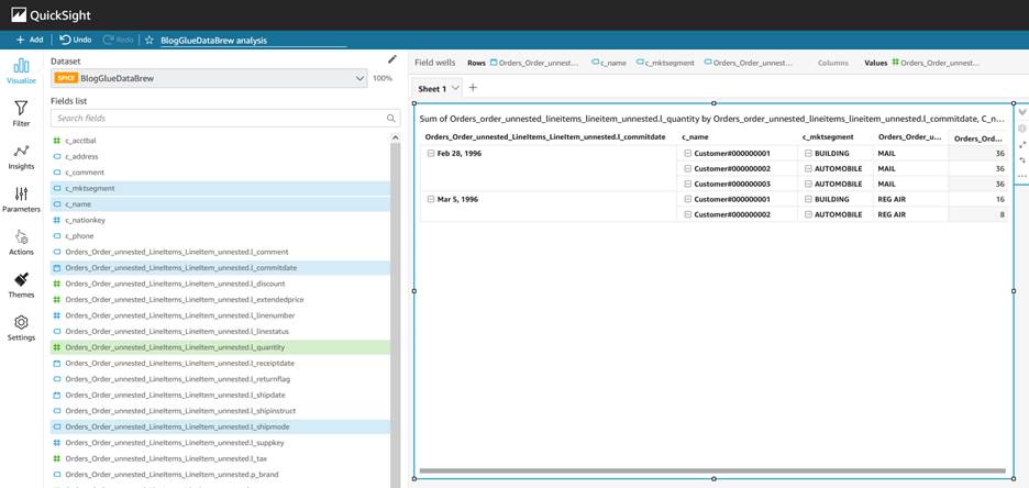
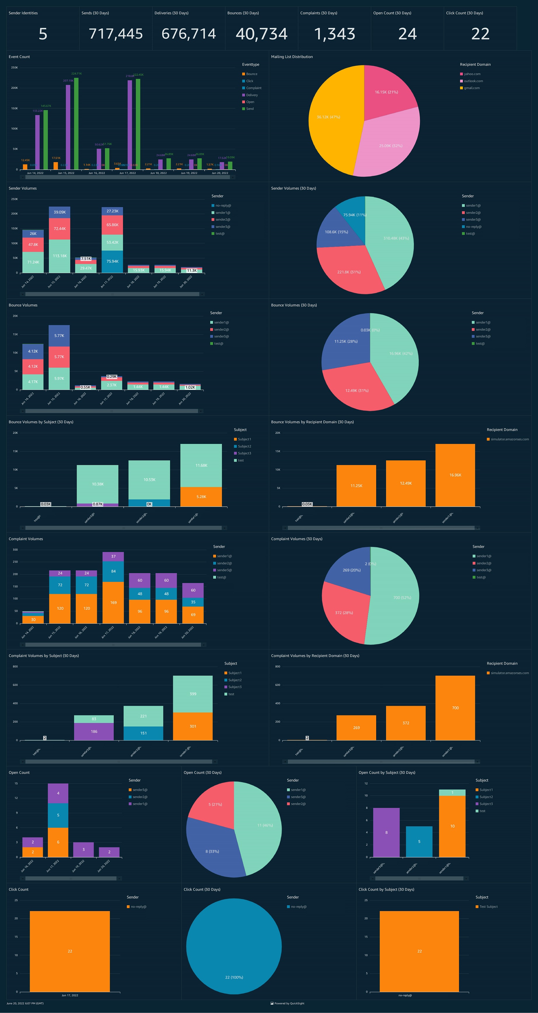
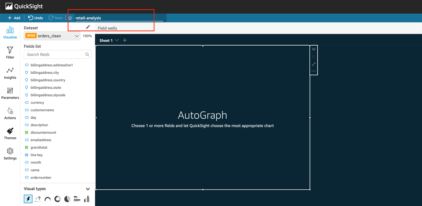
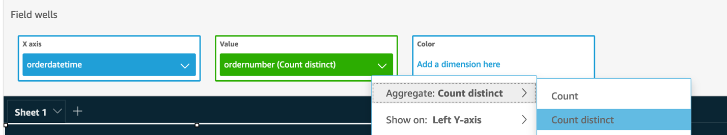
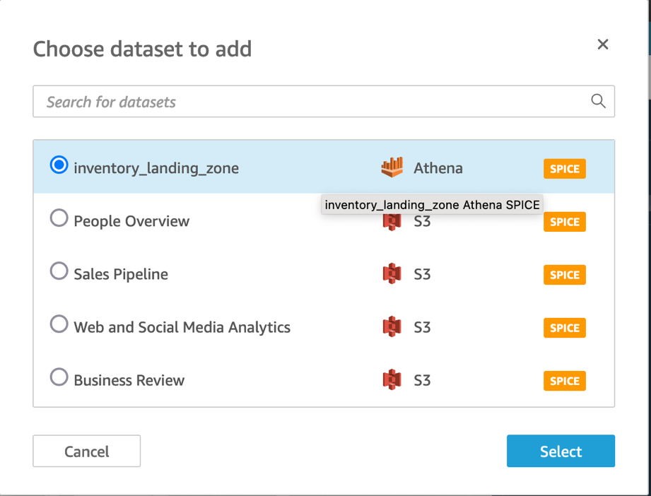
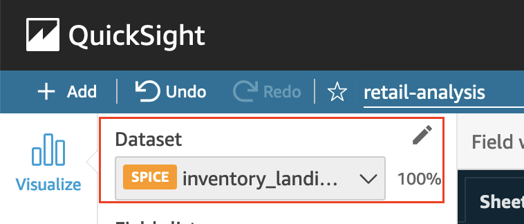
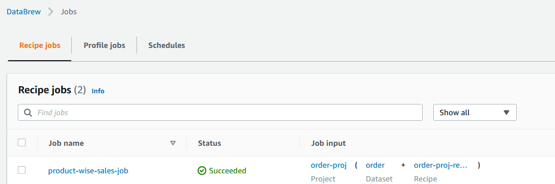
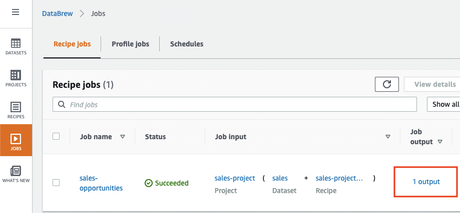
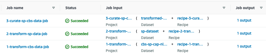
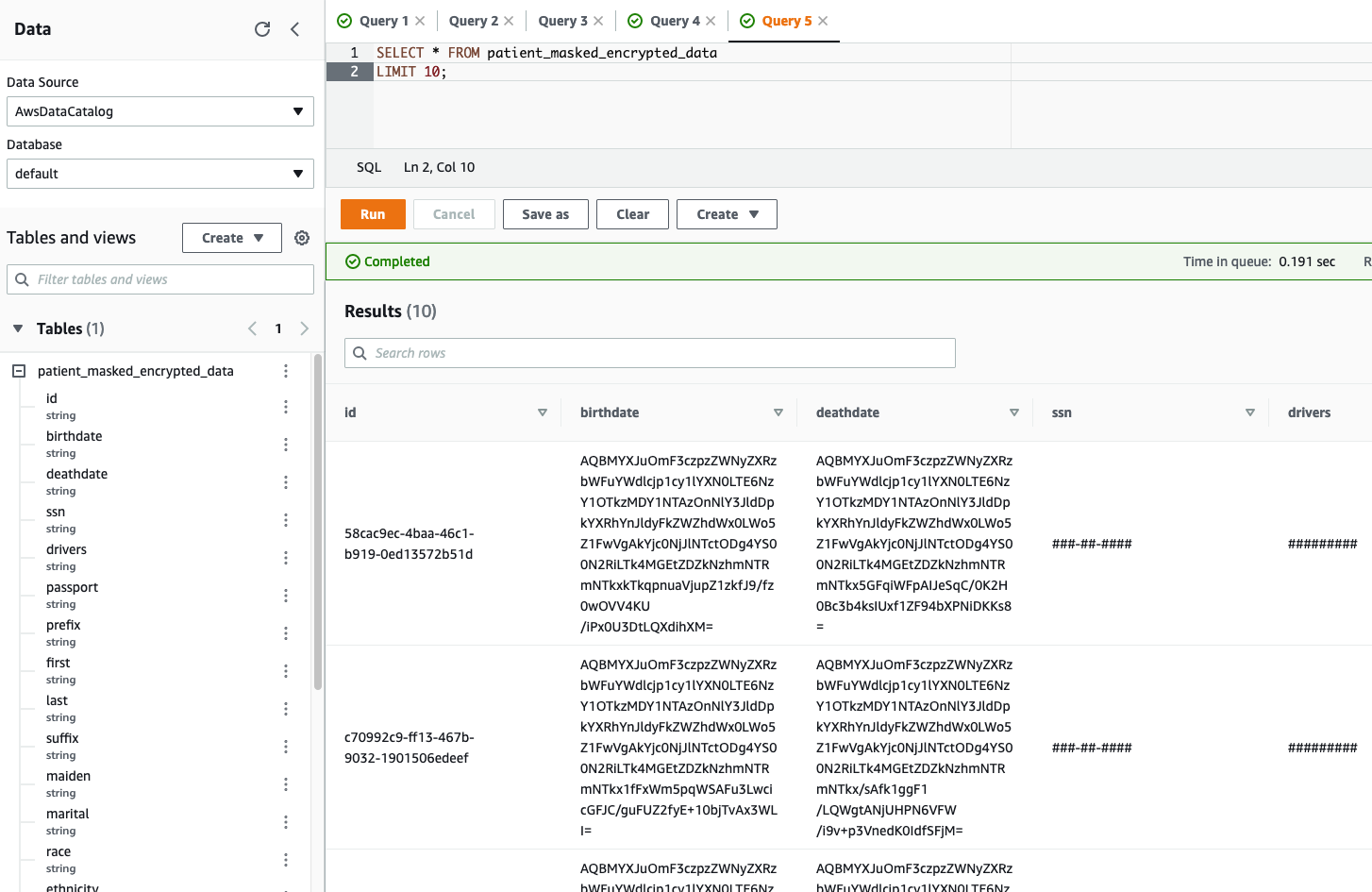
After the batch job runs successfully, you can use OpenSearch Service to run search queries or reports. As shown in the following screenshot, the pipeline masked sensitive fields automatically with no code development efforts.

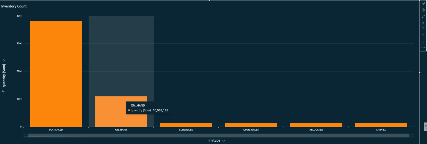
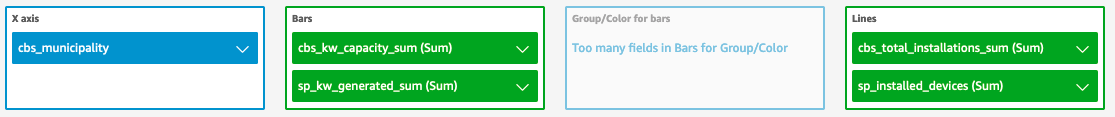
You can identify trends from the operational data, such as the amount of transactions per day filtered by credit card provider, as shown in the preceding screenshot. You can also determine the locations and domains where users make purchases. The transaction_date attribute helps us see these trends over time. The following screenshot shows a record with all of the transaction’s information redacted appropriately.

json masked

For alternate methods on how to load data into Amazon OpenSearch, refer to Loading streaming data into Amazon OpenSearch Service.

Furthermore, sensitive data can also be discovered and masked using other AWS solutions. For example, you could use Amazon Macie to detect sensitive data inside an S3 bucket, and then use Amazon Comprehend to redact the sensitive data that was detected. For more information, refer to Common techniques to detect PHI and PII data using AWS Services.

Conclusion

This post discussed the importance of handling sensitive data within your environment and various methods and architectures to remain compliant while also allowing your organization to scale quickly. You should now have a good understanding of how to detect, mask, or redact and load your data into Amazon OpenSearch Service.


About the authors

Michael Hamilton is a Sr Analytics Solutions Architect focusing on helping enterprise customers modernize and simplify their analytics workloads on AWS. He enjoys mountain biking and spending time with his wife and three children when not working.

Daniel Rozo is a Senior Solutions Architect with AWS supporting customers in the Netherlands. His passion is engineering simple data and analytics solutions and helping customers move to modern data architectures. Outside of work, he enjoys playing tennis and biking.

Modernize your ETL platform with AWS Glue Studio: A case study from BMS

Post Syndicated from Sivaprasad Mahamkali original https://aws.amazon.com/blogs/big-data/modernize-your-etl-platform-with-aws-glue-studio-a-case-study-from-bms/

This post is co-written with Ramesh Daddala, Jitendra Kumar Dash and Pavan Kumar Bijja from Bristol Myers Squibb.

Bristol Myers Squibb (BMS) is a global biopharmaceutical company whose mission is to discover, develop, and deliver innovative medicines that help patients prevail over serious diseases. BMS is consistently innovating, achieving significant clinical and regulatory successes. In collaboration with AWS, BMS identified a business need to migrate and modernize their custom extract, transform, and load (ETL) platform to a native AWS solution to reduce complexities, resources, and investment to upgrade when new Spark, Python, or AWS Glue versions are released. In addition to using native managed AWS services that BMS didn’t need to worry about upgrading, BMS was looking to offer an ETL service to non-technical business users that could visually compose data transformation workflows and seamlessly run them on the AWS Glue Apache Spark-based serverless data integration engine. AWS Glue Studio is a graphical interface that makes it easy to create, run, and monitor ETL jobs in AWS Glue. Offering this service reduced BMS’s operational maintenance and cost, and offered flexibility to business users to perform ETL jobs with ease.

For the past 5 years, BMS has used a custom framework called Enterprise Data Lake Services (EDLS) to create ETL jobs for business users. Although this framework met their ETL objectives, it was difficult to maintain and upgrade. BMS’s EDLS platform hosts over 5,000 jobs and is growing at 15% YoY (year over year). Each time the newer version of Apache Spark (and corresponding AWS Glue version) was released, it required significant operational support and time-consuming manual changes to upgrade existing ETL jobs. Manually upgrading, testing, and deploying over 5,000 jobs every few quarters was time consuming, error prone, costly, and not sustainable. Because another release for the EDLS framework was pending, BMS decided to assess alternate managed solutions to reduce their operational and upgrade challenges.

In this post, we share how BMS will modernize leveraging the success of the proof of concept targeting BMS’s ETL platform using AWS Glue Studio.

Solution overview

This solution addresses BMS’s EDLS requirements to overcome challenges using a custom-built ETL framework that required frequent maintenance and component upgrades (requiring extensive testing cycles), avoid complexity, and reduce the overall cost of the underlying infrastructure derived from the proof of concept. BMS had the following goals:

  • Develop ETL jobs using visual workflows provided by the AWS Glue Studio visual editor. The AWS Glue Studio visual editor is a low-code environment that allows you to compose data transformation workflows, seamlessly run them on the AWS Glue Apache Spark-based serverless data integration engine, and inspect the schema and data results in each step of the job.
  • Migrate over 5,000 existing ETL jobs using native AWS Glue Studio in an automated and scalable manner.

EDLS job steps and metadata

Every EDLS job comprises one or more job steps chained together and run in a predefined order orchestrated by the custom ETL framework. Each job step incorporates the following ETL functions:

  • File ingest – File ingestion enables you to ingest or list files from multiple file sources, like Amazon Simple Storage Service (Amazon S3), SFTP, and more. The metadata holds configurations for the file ingestion step to connect to Amazon S3 or SFTP endpoints and ingest files to target location. It retrieves the specified files and available metadata to show on the UI.
  • Data quality check – The data quality module enables you to perform quality checks on a huge amount of data and generate reports that describe and validate the data quality. The data quality step uses an EDLS ingested source object from Amazon S3 and runs one to many data conformance checks that are configured by the tenant.
  • Data transform join – This is one of the submodules of the data transform module that can perform joins between the datasets using a custom SQL based on the metadata configuration.
  • Database ingest – The database ingestion step is one of the important service components in EDLS, which facilitates you to obtain and import the desired data from the database and export it to a specific file in the location of your choice.
  • Data transform – The data transform module performs various data transformations against the source data using JSON-driven rules. Each data transform capability has its own JSON rule and, based on the specific JSON rule you provide, EDLS performs the data transformation on the files available in the Amazon S3 location.
  • Data persistence – The data persistence module is one of the important service components in EDLS, which enables you to obtain the desired data from the source and persist it to an Amazon Relational Database Service (Amazon RDS) database.

The metadata corresponding to each job step includes ingest sources, transformation rules, data quality checks, and data destinations stored in an RDS instance.

Migration utility

The solution involves building a Python utility that reads EDLS metadata from the RDS database and translating each of the job steps into an equivalent AWS Glue Studio visual editor JSON node representation.

AWS Glue Studio provides two types of transforms:

  • AWS Glue-native transforms – These are available to all users and are managed by AWS Glue.
  • Custom visual transforms – This new functionality allows you to upload custom-built transforms used in AWS Glue Studio. Custom visual transforms expand the managed transforms, enabling you to search and use transforms from the AWS Glue Studio interface.

The following is a high-level diagram depicting the sequence flow of migrating a BMS EDLS job to an AWS Glue Studio visual editor job.

Migrating BMS EDLS jobs to AWS Glue Studio includes the following steps:

  1. The Python utility reads existing metadata from the EDLS metadata database.
  2. For each job step type, based on the job metadata, the Python utility selects either the native AWS Glue transform, if available, or a custom-built visual transform (when the native functionality is missing).
  3. The Python utility parses the dependency information from metadata and builds a JSON object representing a visual workflow represented as a Directed Acyclic Graph (DAG).
  4. The JSON object is sent to the AWS Glue API, creating the AWS Glue ETL job. These jobs are visually represented in the AWS Glue Studio visual editor using a series of sources, transforms (native and custom), and targets.

Sample ETL job generation using AWS Glue Studio

The following flow diagram depicts a sample ETL job that incrementally ingests the source RDBMS data in AWS Glue based on modified timestamps using a custom SQL and merges it into the target data on Amazon S3.

The preceding ETL flow can be represented using the AWS Glue Studio visual editor through a combination of native and custom visual transforms.

Custom visual transform for incremental ingestion

Post POC, BMS and AWS identified there will be a need to leverage custom transforms to execute a subset of jobs leveraging their current EDLS Service where Glue Studio functionality will not be a natural fit. The BMS team’s requirement was to ingest data from various databases without depending on the existence of transaction logs or specific schema, so AWS Database Migration Service (AWS DMS) wasn’t an option for them. AWS Glue Studio provides the native SQL query visual transform, where a custom SQL query can be used to transform the source data. However, in order to query the source database table based on a modified timestamp column to retrieve new and modified records since the last ETL run, the previous timestamp column state needs to be persisted so it can be used in the current ETL run. This needs to be a recurring process and can also be abstracted across various RDBMS sources, including Oracle, MySQL, Microsoft SQL Server, SAP Hana, and more.

AWS Glue provides a job bookmark feature to track the data that has already been processed during a previous ETL run. An AWS Glue job bookmark supports one or more columns as the bookmark keys to determine new and processed data, and it requires that the keys are sequentially increasing or decreasing without gaps. Although this works for many incremental load use cases, the requirement is to ingest data from different sources without depending on any specific schema, so we didn’t use an AWS Glue job bookmark in this use case.

The SQL-based incremental ingestion pull can be developed in a generic way using a custom visual transform using a sample incremental ingestion job from a MySQL database. The incremental data is merged into the target Amazon S3 location in Apache Hudi format using an upsert write operation.

In the following example, we’re using the MySQL data source node to define the connection but the DynamicFrame of the data source itself is not used. The custom transform node (DB incremental ingestion) will act as the source for reading the data incrementally using the custom SQL query and the previously persisted timestamp from the last ingestion.

The transform accepts as input parameters the preconfigured AWS Glue connection name, database type, table name, and custom SQL (parameterized timestamp field).

The following is the sample visual transform Python code:

import boto3
from awsglue import DynamicFrame
from datetime import datetime

region_name = "us-east-1"

dyna_client = boto3.client('dynamodb')
HISTORIC_DATE = datetime(1970,1,1).strftime("%Y-%m-%d %H:%M:%S")
DYNAMODB_TABLE = "edls_run_stats"

def db_incremental(self, transformation_node, con_name, con_type, table_name, sql_query):
    logger = self.glue_ctx.get_logger()

    last_updt_tmst = get_table_last_updt_tmst(logger, DYNAMODB_TABLE, transformation_node)

    logger.info(f"Last updated timestamp from the DynamoDB-> {last_updt_tmst}")

    sql_query = sql_query.format(**{"lastmdfdtmst": last_updt_tmst})

    connection_options_source = {
        "useConnectionProperties": "true",
        "connectionName": con_name,
        "dbtable": table_name,
        "sampleQuery": sql_query
    }

    df = self.glue_ctx.create_dynamic_frame.from_options(connection_type= con_type, connection_options= connection_options_source )
                                         
    return df

DynamicFrame.db_incremental = db_incremental

def get_table_last_updt_tmst(logger, table_name, transformation_node):
    response = dyna_client.get_item(TableName=table_name,
                                    Key={'transformation_node': {'S': transformation_node}}
                                    )
    if 'Item' in response and 'last_updt_tmst' in response['Item']:
        return response['Item']['last_updt_tmst']['S']
    else:
        return HISTORIC_DATE

To merge the source data into the Amazon S3 target, a data lake framework like Apache Hudi or Apache Iceberg can be used, which is natively supported in AWS Glue 3.0 and later.

You can also use Amazon EventBridge to detect the final AWS Glue job state change and update the Amazon DynamoDB table’s last ingested timestamp accordingly.

Build the AWS Glue Studio job using the AWS SDK for Python (Boto3) and AWS Glue API

For the sample ETL flow and the corresponding AWS Glue Studio ETL job we showed earlier, the underlying CodeGenConfigurationNode struct (an AWS Glue job definition pulled using the AWS Command Line Interface (AWS CLI) command aws glue get-job –job-name <jobname>) is represented as a JSON object, shown in the following code:

"CodeGenConfigurationNodes": {<br />"node-1679802581077": {<br />"DynamicTransform": {<br />"Name": "DB Incremental Ingestion",<br />"TransformName": "db_incremental",<br />"Inputs": [<br />"node-1679707801419"<br />],<br />"Parameters": [<br />{<br />"Name": "node_name",<br />"Type": "str",<br />"Value": [<br />"job_123_incr_ingst_table1"<br />],<br />"IsOptional": false<br />},<br />{<br />"Name": "jdbc_url",<br />"Type": "str",<br />"Value": [<br />"jdbc:mysql://database.xxxx.us-west-2.rds.amazonaws.com:3306/db_schema"<br />],<br />"IsOptional": false<br />},<br />{<br />"Name": "db_creds",<br />"Type": "str",<br />"Value": [<br />"creds"<br />],<br />"IsOptional": false<br />},<br />{<br />"Name": "table_name",<br />"Type": "str",<br />"Value": [<br />"tables"<br />],<br />"IsOptional": false<br />}<br />]<br />}<br />}<br />}<br />}

The JSON object (ETL job DAG) represented in the CodeGenConfigurationNode is generated through a series of native and custom transforms with the respective input parameter arrays. This can be accomplished using Python JSON encoders that serialize the class objects to JSON and subsequently create the AWS Glue Studio visual editor job using the Boto3 library and AWS Glue API.

Inputs required to configure the AWS Glue transforms are sourced from the EDLS jobs metadata database. The Python utility reads the metadata information, parses it, and configures the nodes automatically.

The order and sequencing of the nodes is sourced from the EDLS jobs metadata, with one node becoming the input to one or more downstream nodes building the DAG flow.

Benefits of the solution

The migration path will help BMS achieve their core objectives of decomposing their existing custom ETL framework to modular, visually configurable, less complex, and easily manageable pipelines using visual ETL components. The utility aids the migration of the legacy ETL pipelines to native AWS Glue Studio jobs in an automated and scalable manner.

With consistent out-of-the box visual ETL transforms in the AWS Glue Studio interface, BMS will be able to build sophisticated data pipelines without having to write code.

The custom visual transforms will extend AWS Glue Studio capabilities and fulfill some of the BMS ETL requirements where the native transforms are missing that functionality. Custom transforms will help define, reuse, and share business-specific ETL logic among all the teams. The solution increases the consistency between teams and keeps the ETL pipelines up to date by minimizing duplicate effort and code.

With minor modifications, the migration utility can be reused to automate migration of pipelines during future AWS Glue version upgrades.

Conclusion

The successful outcome of this proof of concept has shown that migrating over 5,000 jobs from BMS’s custom application to native AWS services can deliver significant productivity gains and cost savings. By moving to AWS, BMS will be able to reduce the effort required to support AWS Glue, improve DevOps delivery, and save an estimated 58% on AWS Glue spend.

These results are very promising, and BMS is excited to embark on the next phase of the migration. We believe that this project will have a positive impact on BMS’s business and help us achieve our strategic goals.


About the authors

Sivaprasad Mahamkali is a Senior Streaming Data Engineer at AWS Professional Services. Siva leads customer engagements related to real-time streaming solutions, data lakes, analytics using opensource and AWS services. Siva enjoys listening to music and loves to spend time with his family.

Dan Gibbar is a Senior Engagement Manager at AWS Professional Services. Dan leads healthcare and life science engagements collaborating with customers and partners to deliver outcomes. Dan enjoys the outdoors, attempting triathlons, music and spending time with family.

Shrinath Parikh as a Senior Cloud Data Architect with AWS. He works with customers around the globe to assist them with their data analytics, data lake, data lake house, serverless, governance and NoSQL use cases. In Shrinath’s off time, he enjoys traveling, spending time with family and learning/building new tools using cutting edge technologies.

Ramesh Daddala is a Associate Director at BMS. Ramesh leads enterprise data engineering engagements related to enterprise data lake services (EDLs) and collaborating with Data partners to deliver and support enterprise data engineering and ML capabilities. Ramesh enjoys the outdoors, traveling and loves to spend time with family.

Jitendra Kumar Dash is a Senior Cloud Architect at BMS with expertise in hybrid cloud services, Infrastructure Engineering, DevOps, Data Engineering, and Data Analytics solutions. He is passionate about food, sports, and adventure.

Pavan Kumar Bijja is a Senior Data Engineer at BMS. Pavan enables data engineering and analytical services to BMS Commercial domain using enterprise capabilities. Pavan leads enterprise metadata capabilities at BMS. Pavan loves to spend time with his family, playing Badminton and Cricket.

Shovan Kanjilal is a Senior Data Lake Architect working with strategic accounts in AWS Professional Services. Shovan works with customers to design data and machine learning solutions on AWS.

Clean up your Excel and CSV files without writing code using AWS Glue DataBrew

Post Syndicated from Ismail Makhlouf original https://aws.amazon.com/blogs/big-data/clean-up-your-excel-and-csv-files-without-writing-code-using-aws-glue-databrew/

Managing data within an organization is complex. Handling data from outside the organization adds even more complexity. As the organization receives data from multiple external vendors, it often arrives in different formats, typically Excel or CSV files, with each vendor using their own unique data layout and structure. In this blog post, we’ll explore a solution that streamlines this process by leveraging the capabilities of AWS Glue DataBrew.

DataBrew is an excellent tool for data quality and preprocessing. You can use its built-in transformations, recipes, as well as integrations with the AWS Glue Data Catalog and Amazon Simple Storage Service (Amazon S3) to preprocess the data in your landing zone, clean it up, and send it downstream for analytical processing.

In this post, we demonstrate the following:

  • Extracting non-transactional metadata from the top rows of a file and merging it with transactional data
  • Combining multi-line rows into single-line rows
  • Extracting unique identifiers from within strings or text

Solution overview

For this use case, imagine you’re a data analyst working at your organization. The sales leadership have requested a consolidated view of the net sales they are making from each of the organization’s suppliers. Unfortunately, this information is not available in a database. The sales data comes from each supplier in layouts like the following example.

However, with hundreds of resellers, manually extracting the information at the top is not feasible. Your goal is to clean up and flatten the data into the following output layout.

image2

To achieve this, you can use pre-built transformations in DataBrew to quickly get the data in the layout you want.

Prerequisites

For this walkthrough, you should have the following prerequisites:

Connect to the dataset

The first thing we need to do is upload the input dataset to Amazon S3. Create an S3 bucket for the project and create a folder to upload the raw input data. The output data will be stored in another folder in a later step.

Next, we need to connect DataBrew to our CSV file. We create what we call a dataset, which
is an artifact that points to whatever data source we will be using. Navigate to “Datasets” on
the left hand menu.

Ensure the Column header values field is set to Add default header. The input CSV has an irregular format, so the first row will not have the needed column values.

Create a project

To create a new project, complete the following steps:

  1. On the DataBrew console, choose Projects in the navigation pane.
  2. Choose Create project.
  3. For Project name, enter FoodMartSales-AllUpProject.
  4. For Attached recipe, choose Create new recipe.
  5. For Recipe name, enter FoodMartSales-AllUpProject-recipe.
  6. For Select a dataset, select My datasets.
  7. Select the FoodMartSales-AllUp dataset.
  8. Under Permissions, for Role name, choose the IAM role you created as a prerequisite or create a new role.
  9. Choose Create project.

After the project is opened, an interactive session is created where you can author transformations on a sample of the data.

Extract non-transactional metadata from within the contents of the file and merge it with transactional data

In this section, we consider data that has metadata on the first few rows of the file, followed by transactional data. We walk through how to extract data relevant to the whole file from the top of the document and combine it with the transactional data into one flat table.

Extract metadata from the header and remove invalid rows

Complete the following steps to extract metadata from the header:

  1. Choose Conditions and then choose IF.
  2. For Matching conditions, choose Match all conditions.
  3. For Source, choose Value of and Column_1.
  4. For Logical condition, choose Is exactly.
  5. For Enter a value, choose Enter custom value and enter RESELLER NAME.
  6. For Flag result value as, choose Custom value.
  7. For Value if true, choose Select source column and set Value of to Column_2.
  8. For Value if false, choose Enter custom value and enter INVALID.
  9. Choose Apply.

Your dataset should now look like the following screenshot, with the Reseller Name value extracted to a column by itself.

Next, you remove invalid rows and fill the rows with the Reseller Name value.

  1. Choose Clean and then choose Custom values.
  2. For Source column, choose ResellerName.
  3. For Specify values to remove, choose Custom value.
  4. For Values to remove, choose Invalid.
  5. For Apply transform to, choose All rows.
  6. Choose Apply.
  7. Choose Missing and then choose Fill with most frequent value.
  8. For Source column, choose FirstTransactionDate.
  9. For Missing value action, choose Fill with most frequent value.
  10. For Apply transform to, choose All rows.
  11. Choose Apply.

Your dataset should now look like the following screenshot, with the Reseller Name value extracted to a column by itself.

Repeat the same steps in this section for the rest of the metadata, including Reseller Email Address, Reseller ID, and First Transaction Date.

Promote column headers and clean up data

To promote column headers, complete the following steps:

  1. Reorder the columns to put the metadata columns to the left of the dataset by choosing Column, Move column, and Start of the table.
  2. Rename the columns with the appropriate names.

Now you can clean up some columns and rows.

  1. Delete unnecessary columns, such as Column_7.

You can also delete invalid rows by filtering out records that don’t have a transaction date value.

  1. Choose the ABC icon on the menu of the Transaction_Date column and choose date.

  2. For Handle invalid values, select Delete rows, then choose Apply.

The dataset should now have the metadata extracted and the column headers promoted.

Combine multi-line rows into single-line rows

The next issue to address is transactions pertaining to the same row that are split across multiple lines. In the following steps, we extract the needed data from the rows and merge it into single-line transactions. For this example specifically, the Reseller Margin data is split across two lines.


Complete the following steps to get the Reseller Margin value on the same line as the corresponding transaction. First, we identify the Reseller Margin rows and store them in a temporary column.

  1. Choose Conditions and then choose IF.
  2. For Matching conditions, choose Match all conditions.
  3. For Source, choose Value of and Transaction_ID.
  4. For Logical condition, choose Contains.
  5. For Enter a value, choose Enter custom value and enter Reseller Margin.
  6. For Flag result value as, choose Custom value.
  7. For Value if true, choose Select source column set Value of to TransactionAmount.
  8. For Value if false, choose Enter custom value and enter Invalid.
  9. For Destination column, choose ResellerMargin_Temp.
  10. Choose Apply.

Next, you shift the Reseller Margin value up one row.

  1. Choose Functions and then choose NEXT.
  2. For Source column, choose ResellerMargin_Temp.
  3. For Number of rows, enter 1.
  4. For Destination column, choose ResellerMargin.
  5. For Apply transform to, choose All rows.
  6. Choose Apply.

Next, delete the invalid rows.

  1. Choose Missing and then choose Remove missing rows.
  2. For Source column, choose TransactionDate.
  3. For Missing value action, choose Delete rows with missing values.
  4. For Apply transform to, choose All rows.
  5. Choose Apply.

Your dataset should now look like the following screenshot, with the Reseller Margin value extracted to a column by itself.

With the data structured properly, we can move on to mining the cleaned data.

Extract unique identifiers from within strings and text

Many types of data contain important information stored as unstructured text in a cell. In this section, we look at how to extract this data. Within the sample dataset, the BankTransferText column has valuable information around our resellers’ registered bank account numbers as well as the currency of the transaction, namely IBAN, SWIFT Code, and Currency.

Complete the following steps to extract IBAN, SWIFT code, and Currency into separate columns. First, you extract the IBAN number from the text using a regular expression (regex).

  1. Choose Extract and then choose Custom value or pattern.
  2. For Create column options, choose Extract values.
  3. For Source column, choose BankTransferText.
  4. For Extract options, choose Custom value or pattern.
  5. For Values to extract, enter [a-zA-Z][a-zA-Z][0-9]{2}[A-Z0-9]{1,30}.
  6. For Destination column, choose IBAN.
  7. For Apply transform to, choose All rows.
  8. Choose Apply.
  9. Extract the SWIFT code from the text using a regex following the same steps used to extract the IBAN number, but using the following regex instead: (?!^)(SWIFT Code: )([A-Z]{2}[A-Z0-9]+).

Next, remove the SWIFT Code: label from the extracted text.

  1. Choose Remove and then choose Custom values.
  2. For Source column, choose SWIFT Code.
  3. For Specify values to remove, choose Custom value.
  4. For Apply transform to, choose All rows.
  5. Extract the currency from the text using a regex following the same steps used to extract the IBAN number, but using the following regex instead: (?!^)(Currency: )([A-Z]{3}).
  6. Remove the Currency: label from the extracted text following the same steps used to remove the SWIFT Code: label.

You can clean up by deleting any unnecessary columns.

  1. Choose Column and then choose Delete.
  2. For Source columns, choose BankTransferText.
  3. Choose Apply.
  4. Repeat for any remaining columns.

Your dataset should now look like the following screenshot, with IBAN, SWIFT Code, and Currency extracted to separate columns.

Write the transformed data to Amazon S3

With all the steps captured in the recipe, the last step is to write the transformed data to Amazon S3.

  1. On the DataBrew console, choose Run job.
  1. For Job name, enter FoodMartSalesToDataLake.
  2. For Output to, choose Amazon S3.
  3. For File type, choose CSV.
  4. For Delimiter, choose Comma (,).
  5. For Compression, choose None.
  6. For S3 bucket owners’ account, select Current AWS account.
  7. For S3 location, enter s3://{name of S3 bucket}/clean/.
  8. For Role name, choose the IAM role created as a prerequisite or create a new role.
  9. Choose Create and run job.
  10. Go to the Jobs tab and wait for the job to complete.
  11. Navigate to the job output folder on the Amazon S3 console.
  12. Download the CSV file and view the transformed output.

Your dataset should look similar to the following screenshot.

Clean up

To optimize cost, make sure to clean up the resources deployed for this project by completing the following steps:

  1. Delete every DataBrew project along with their linked recipes.
  2. Delete all the DataBrew datasets.
  3. Delete the contents in your S3 bucket.
  4. Delete the S3 bucket.

Conclusion

The reality of exchanging data with suppliers is that we can’t always control the shape of the input data. With DataBrew, we can use a list of pre-built transformations and repeatable steps to transform incoming data into a desired layout and extract relevant data and insights from Excel or CSV files. Start using DataBrew today and transform 3 rd party files into structured datasets ready for consumption by your business.


About the Author

Ismail Makhlouf is a Senior Specialist Solutions Architect for Data Analytics at AWS. Ismail focuses on architecting solutions for organizations across their end-to-end data analytics estate, including batch and real-time streaming, big data, data warehousing, and data lake workloads. He primarily works with direct-to-consumer platform companies in the ecommerce, FinTech, PropTech, and HealthTech space to achieve their business objectives with well-architected data platforms.

Empower your Jira data in a data lake with Amazon AppFlow and AWS Glue

Post Syndicated from Tom Romano original https://aws.amazon.com/blogs/big-data/empower-your-jira-data-in-a-data-lake-with-amazon-appflow-and-aws-glue/

In the world of software engineering and development, organizations use project management tools like Atlassian Jira Cloud. Managing projects with Jira leads to rich datasets, which can provide historical and predictive insights about project and development efforts.

Although Jira Cloud provides reporting capability, loading this data into a data lake will facilitate enrichment with other business data, as well as support the use of business intelligence (BI) tools and artificial intelligence (AI) and machine learning (ML) applications. Companies often take a data lake approach to their analytics, bringing data from many different systems into one place to simplify how the analytics are done.

This post shows you how to use Amazon AppFlow and AWS Glue to create a fully automated data ingestion pipeline that will synchronize your Jira data into your data lake. Amazon AppFlow provides software as a service (SaaS) integration with Jira Cloud to load the data into your AWS account. AWS Glue is a serverless data discovery, load, and transformation service that will prepare data for consumption in BI and AI/ML activities. Additionally, this post strives to achieve a low-code and serverless solution for operational efficiency and cost optimization, and the solution supports incremental loading for cost optimization.

Solution overview

This solution uses Amazon AppFlow to retrieve data from the Jira Cloud. The data is synchronized to an Amazon Simple Storage Service (Amazon S3) bucket using an initial full download and subsequent incremental downloads of changes. When new data arrives in the S3 bucket, an AWS Step Functions workflow is triggered that orchestrates extract, transform, and load (ETL) activities using AWS Glue crawlers and AWS Glue DataBrew. The data is then available in the AWS Glue Data Catalog and can be queried by services such as Amazon Athena, Amazon QuickSight, and Amazon Redshift Spectrum. The solution is completely automated and serverless, resulting in low operational overhead. When this setup is complete, your Jira data will be automatically ingested and kept up to date in your data lake!

The following diagram illustrates the solution architecture.

The Jira Appflow Architecture is shown. The Jira Cloud data is retrieved by Amazon AppFlow and is stored in Amazon S3. This triggers an Amazon EventBridge event that runs an AWS Step Functions workflow. The workflow uses AWS Glue to catalog and transform the data, The data is then queried with QuickSight.

The Step Functions workflow orchestrates the following ETL activities, resulting in two tables:

  • An AWS Glue crawler collects all downloads into a single AWS Glue table named jira_raw. This table is comprised of a mix of full and incremental downloads from Jira, with many versions of the same records representing changes over time.
  • A DataBrew job prepares the data for reporting by unpacking key-value pairs in the fields, as well as removing depreciated records as they are updated in subsequent change data captures. This reporting-ready data will available in an AWS Glue table named jira_data.

The following figure shows the Step Functions workflow.

A diagram represents the AWS Step Functions workflow. It contains the steps to run an AWS Crawler, wait for it's completion, and then run a AWS Glue DataBrew data transformation job.

Prerequisites

This solution requires the following:

  • Administrative access to your Jira Cloud instance, and an associated Jira Cloud developer account.
  • An AWS account and a login with access to the AWS Management Console. Your login will need AWS Identity and Access Management (IAM) permissions to create and access the resources in your AWS account.
  • Basic knowledge of AWS and working knowledge of Jira administration.

Configure the Jira Instance

After logging in to your Jira Cloud instance, you establish a Jira project with associated epics and issues to download into a data lake. If you’re starting with a new Jira instance, it helps to have at least one project with a sampling of epics and issues for the initial data download, because it allows you to create an initial dataset without errors or missing fields. Note that you may have multiple projects as well.

An image show a Jira Cloud example, with several issues arranged in a Kansan board.

After you have established your Jira project and populated it with epics and issues, ensure you also have access to the Jira developer portal. In later steps, you use this developer portal to establish authentication and permissions for the Amazon AppFlow connection.

Provision resources with AWS CloudFormation

For the initial setup, you launch an AWS CloudFormation stack to create an S3 bucket to store data, IAM roles for data access, and the AWS Glue crawler and Data Catalog components. Complete the following steps:

  1. Sign in to your AWS account.
  2. Click Launch Stack:
  3. For Stack name, enter a name for the stack (the default is aws-blog-jira-datalake-with-AppFlow).
  4. For GlueDatabaseName, enter a unique name for the Data Catalog database to hold the Jira data table metadata (the default is jiralake).
  5. For InitialRunFlag, choose Setup. This mode will scan all data and disable the change data capture (CDC) features of the stack. (Because this is the initial load, the stack needs an initial data load before you configure CDC in later steps.)
  6. Under Capabilities and transforms, select the acknowledgement check boxes to allow IAM resources to be created within your AWS account.
  7. Review the parameters and choose Create stack to deploy the CloudFormation stack. This process will take around 5–10 minutes to complete.
    An image depicts the Amazon CloudFormation configuration steps, including setting a stack name, setting parameters to "jiralake" and "Setup" mode, and checking all IAM capabilities requested.
  8. After the stack is deployed, review the Outputs tab for the stack and collect the following values to use when you set up Amazon AppFlow:
    • Amazon AppFlow destination bucket (o01AppFlowBucket)
    • Amazon AppFlow destination bucket path (o02AppFlowPath)
    • Role for Amazon AppFlow Jira connector (o03AppFlowRole)
      An image demonstrating the Amazon Cloudformation "Outputs" tab, highlighting the values to add to the Amazon AppFlow configuration.

Configure Jira Cloud

Next, you configure your Jira Cloud instance for access by Amazon AppFlow. For full instructions, refer to Jira Cloud connector for Amazon AppFlow. The following steps summarize these instructions and discuss the specific configuration to enable OAuth in the Jira Cloud:

  1. Open the Jira developer portal.
  2. Create the OAuth 2 integration from the developer application console by choosing Create an OAuth 2.0 Integration. This will provide a login mechanism for AppFlow.
  3. Enable fine-grained permissions. See Recommended scopes for the permission settings to grant AppFlow appropriate access to your Jira instance.
  4. Add the following permission scopes to your OAuth app:
    1. manage:jira-configuration
    2. read:field-configuration:jira
  5. Under Authorization, set the Call Back URL to return to Amazon AppFlow with the URL https://us-east-1.console.aws.amazon.com/AppFlow/oauth.
  6. Under Settings, note the client ID and secret to use in later steps to set up authentication from Amazon AppFlow.

Create the Amazon AppFlow Jira Cloud connection

In this step, you configure Amazon AppFlow to run a one-time full data fetch of all your data, establishing the initial data lake:

  1. On the Amazon AppFlow console, choose Connectors in the navigation pane.
  2. Search for the Jira Cloud connector.
  3. Choose Create flow on the connector tile to create the connection to your Jira instance.
    An image of Amazon AppFlor, showing the search for the "Jira Cloud" connector.
  4. For Flow name, enter a name for the flow (for example, JiraLakeFlow).
  5. Leave the Data encryption setting as the default.
  6. Choose Next.
    The Amazon AppFlow Jira connector configuration, showing the Flow name set to "JiraLakeFlow" and clicking the "next" button.
  7. For Source name, keep the default of Jira Cloud.
  8. Choose Create new connection under Jira Cloud connection.
  9. In the Connect to Jira Cloud section, enter the values for Client ID, Client secret, and Jira Cloud Site that you collected earlier. This provides the authentication from AppFlow to Jira Cloud.
  10. For Connection Name, enter a connection name (for example, JiraLakeCloudConnection).
  11. Choose Connect. You will be prompted to allow your OAuth app to access your Atlassian account to verify authentication.
    An image of the Amazon AppFlow conflagration, reflecting the completion of the prior steps.
  12. In the Authorize App window that pops up, choose Accept.
  13. With the connection created, return to the Configure flow section on the Amazon AppFlow console.
  14. For API version, choose V2 to use the latest Jira query API.
  15. For Jira Cloud object, choose Issue to query and download all issues and associated details.
    An image of the Amazon AppFlow configuration, reflecting the completion of the prior steps.
  16. For Destination Name in the Destination Details section, choose Amazon S3.
  17. For Bucket details, choose the S3 bucket name that matches the Amazon AppFlow destination bucket value that you collected from the outputs of the CloudFormation stack.
  18. Enter the Amazon AppFlow destination bucket path to complete the full S3 path. This will send the Jira data to the S3 bucket created by the CloudFormation script.
  19. Leave Catalog your data in the AWS Glue Data Catalog unselected. The CloudFormation script uses an AWS Glue crawler to update the Data Catalog in a different manner, grouping all the downloads into a common table, so we disable the update here.
  20. For File format settings, select Parquet format and select Preserve source data types in Parquet output. Parquet is a columnar format to optimize subsequent querying.
  21. Select Add a timestamp to the file name for Filename preference. This will allow you to easily find data files downloaded at a specific date and time.
    An image of the Amazon AppFlow configuration, reflecting the completion of the prior steps.
  22. For now, select Run on Demand for the Flow trigger to run the full load flow manually. You will schedule downloads in a later step when implementing CDC.
  23. Choose Next.
    An image of the Amazon AppFlow Flow Trigger configuration, reflecting the completion of the prior steps.
  24. On the Map data fields page, select Manually map fields.
  25. For Source to destination field mapping, choose the drop-down box under Source field name and select Map all fields directly. This will bring down all fields as they are received, because we will instead implement data preparation in later steps.
    An image of the Amazon AppFlow configuration, reflecting the completion of steps 24 & 25.
  26. Under Partition and aggregation settings, you can set up the partitions in a way that works for your use case. For this example, we use a daily partition, so select Date and time and choose Daily.
  27. For Aggregation settings, leave it as the default of Don’t aggregate.
  28. Choose Next.
    An image of the Amazon AppFlow configuration, reflecting the completion of steps 26-28.
  29. On the Add filters page, you can create filters to only download specific data. For this example, you download all the data, so choose Next.
  30. Review and choose Create flow.
  31. When the flow is created, choose Run flow to start the initial data seeding. After some time, you should receive a banner indicating the run finished successfully.
    An image of the Amazon AppFlow configuration, reflecting the completion of step 31.

Review seed data

At this stage in the process, you now have data in your S3 environment. When new data files are created in the S3 bucket, it will automatically run an AWS Glue crawler to catalog the new data. You can see if it’s complete by reviewing the Step Functions state machine for a Succeeded run status. There is a link to the state machine on the CloudFormation stack’s Resources tab, which will redirect you to the Step Functions state machine.

A image showing the CloudFormation resources tab of the stack, with a link to the AWS Step Functions workflow.

When the state machine is complete, it’s time to review the raw Jira data with Athena. The database is as you specified in the CloudFormation stack (jiralake by default), and the table name is jira_raw. If you kept the default AWS Glue database name of jiralake, the Athena SQL is as follows:

SELECT * FROM "jiralake"."jira_raw" limit 10;

If you explore the data, you’ll notice that most of the data you would want to work with is actually packed into a column called fields. This means the data is not available as columns in your Athena queries, making it harder to select, filter, and sort individual fields within an Athena SQL query. This will be addressed in the next steps.

An image demonstrating the Amazon Athena query SELECT * FROM "jiralake"."jira_raw" limit 10;

Set up CDC and unpack the fields columns

To add the ongoing CDC and reformat the data for analytics, we introduce a DataBrew job to transform the data and filter to the most recent version of each record as changes come in. You can do this by updating the CloudFormation stack with a flag that includes the CDC and data transformation steps.

  1. On the AWS CloudFormation console, return to the stack.
  2. Choose Update.
  3. Select Use current template and choose Next.
    An image showing Amazon CloudFormation, with steps 1-3 complete.
  4. For SetupOrCDC, choose CDC, then choose Next. This will enable both the CDC steps and the data transformation steps for the Jira data.
    An image showing Amazon CloudFormation, with step 4 complete.
  5. Continue choosing Next until you reach the Review section.
  6. Select I acknowledge that AWS CloudFormation might create IAM resources, then choose Submit.
    An image showing Amazon CloudFormation, with step 5-6 complete.
  7. Return to the Amazon AppFlow console and open your flow.
  8. On the Actions menu, choose Edit flow. We will now edit the flow trigger to run an incremental load on a periodic basis.
  9. Select Run flow on schedule.
  10. Configure the desired repeats, as well as start time and date. For this example, we choose Daily for Repeats and enter 1 for the number of days you’ll have the flow trigger. For Starting at, enter 01:00.
  11. Select Incremental transfer for Transfer mode.
  12. Choose Updated on the drop-down menu so that changes will be captured based on when the records were updated.
  13. Choose Save. With these settings in our example, the run will happen nightly at 1:00 AM.
    An image showing the Flow Trigger, with incremental transfer selected.

Review the analytics data

When the next incremental load occurs that results in new data, the Step Functions workflow will start the DataBrew job and populate a new staged analytical data table named jira_data in your Data Catalog database. If you don’t want to wait, you can trigger the Step Functions workflow manually.

The DataBrew job performs data transformation and filtering tasks. The job unpacks the key-values from the Jira JSON data and the raw Jira data, resulting in a tabular data schema that facilitates use with BI and AI/ML tools. As Jira items are changed, the changed item’s data is resent, resulting in multiple versions of an item in the raw data feed. The DataBrew job filters the raw data feed so that the resulting data table only contains the most recent version of each item. You could enhance this DataBrew job to further customize the data for your needs, such as renaming the generic Jira custom field names to reflect their business meaning.

When the Step Functions workflow is complete, we can query the data in Athena again using the following query:

SELECT * FROM "jiralake"."jira_data" limit 10;

You can see that in our transformed jira_data table, the nested JSON fields are broken out into their own columns for each field. You will also notice that we’ve filtered out obsolete records that have been superseded by more recent record updates in later data loads so the data is fresh. If you want to rename custom fields, remove columns, or restructure what comes out of the nested JSON, you can modify the DataBrew recipe to accomplish this. At this point, the data is ready to be used by your analytics tools, such as Amazon QuickSight.

An image demonstrating the Amazon Athena query SELECT * FROM "jiralake"."jira_data" limit 10;

Clean up

If you would like to discontinue this solution, you can remove it with the following steps:

  1. On the Amazon AppFlow console, deactivate the flow for Jira, and optionally delete it.
  2. On the Amazon S3 console, select the S3 bucket for the stack, and empty the bucket to delete the existing data.
  3. On the AWS CloudFormation console, delete the CloudFormation stack that you deployed.

Conclusion

In this post, we created a serverless incremental data load process for Jira that will synchronize data while handling custom fields using Amazon AppFlow, AWS Glue, and Step Functions. The approach uses Amazon AppFlow to incrementally load the data into Amazon S3. We then use AWS Glue and Step Functions to manage the extraction of the Jira custom fields and load them in a format to be queried by analytics services such as Athena, QuickSight, or Redshift Spectrum, or AI/ML services like Amazon SageMaker.

To learn more about AWS Glue and DataBrew, refer to Getting started with AWS Glue DataBrew. With DataBrew, you can take the sample data transformation in this project and customize the output to meet your specific needs. This could include renaming columns, creating additional fields, and more.

To learn more about Amazon AppFlow, refer to Getting started with Amazon AppFlow. Note that Amazon AppFlow supports integrations with many SaaS applications in addition to the Jira Cloud.

To learn more about orchestrating flows with Step Functions, see Create a Serverless Workflow with AWS Step Functions and AWS Lambda. The workflow could be enhanced to load the data into a data warehouse, such as Amazon Redshift, or trigger a refresh of a QuickSight dataset for analytics and reporting.

In future posts, we will cover how to unnest parent-child relationships within the Jira data using Athena and how to visualize the data using QuickSight.


About the Authors

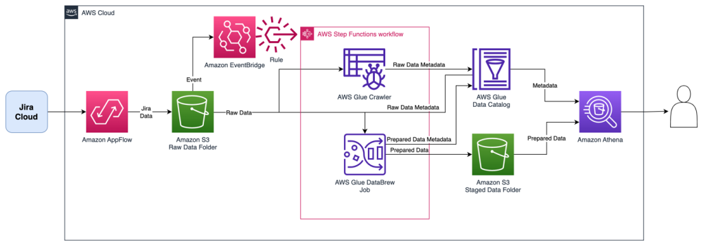
Tom Romano is a Sr. Solutions Architect for AWS World Wide Public Sector from Tampa, FL, and assists GovTech and EdTech customers as they create new solutions that are cloud native, event driven, and serverless. He is an enthusiastic Python programmer for both application development and data analytics, and is an Analytics Specialist. In his free time, Tom flies remote control model airplanes and enjoys vacationing with his family around Florida and the Caribbean.

Shane Thompson is a Sr. Solutions Architect based out of San Luis Obispo, California, working with AWS Startups. He works with customers who use AI/ML in their business model and is passionate about democratizing AI/ML so that all customers can benefit from it. In his free time, Shane loves to spend time with his family and travel around the world.

Use AWS Glue DataBrew recipes in your AWS Glue Studio visual ETL jobs

Post Syndicated from Gonzalo Herreros original https://aws.amazon.com/blogs/big-data/use-aws-glue-databrew-recipes-in-your-aws-glue-studio-visual-etl-jobs/

AWS Glue Studio is now integrated with AWS Glue DataBrew. AWS Glue Studio is a graphical interface that makes it easy to create, run, and monitor extract, transform, and load (ETL) jobs in AWS Glue. DataBrew is a visual data preparation tool that enables you to clean and normalize data without writing any code. The over 200 transformations it provides are now available to be used in an AWS Glue Studio visual job.

In DataBrew, a recipe is a set of data transformation steps that you can author interactively in its intuitive visual interface. In this post, you’ll see how to use build a recipe in DataBrew and then apply it as part of an AWS Glue Studio visual ETL job.

Existing DataBrew users will also benefit from this integration—you can now run your recipes as part of a larger visual workflow with all the other components AWS Glue Studio provides, in addition to being able to use advanced job configuration and the latest AWS Glue engine version.

This integration brings distinct benefits to the existing users of both tools:

  • You have a centralized view in AWS Glue Studio of the overall ETL diagram, end to end
  • You can interactively define a recipe, seeing values, statistics, and distribution on the DataBrew console, then reuse that tested and versioned processing logic in AWS Glue Studio visual jobs
  • You can orchestrate multiple DataBrew recipes in an AWS Glue ETL job or even multiple jobs using AWS Glue workflows
  • DataBrew recipes can now use AWS Glue job features such as bookmarks for incremental data processing, automatic retries, auto scale, or grouping small files for greater efficiency

Solution overview

In our fictitious use case, the requirement is to clean up a synthetic medical claims dataset created for this post, which has some data quality issues introduced on purpose to demonstrate the DataBrew capabilities on data preparation. Then the claims data is ingested into the catalog (so it’s visible to analysts), after enriching it with some relevant details about the corresponding medical providers coming from a separate source.

The solution consists of an AWS Glue Studio visual job that reads two CSV files with claims and providers, respectively. The job applies a recipe of the first one to address the quality issues, select columns from the second one, join both datasets, and finally store the result on Amazon Simple Storage Service (Amazon S3), creating a table on the catalog so the output data can be used by other tools like Amazon Athena.

Create a DataBrew recipe

Start by registering the data store for the claims file. This will allow you to build the recipe in its interactive editor using the actual data so you can evaluate the result of the transformations as you define them.

  1. Download the claims CSV file using the following link: alabama_claims_data_Jun2023.csv.
  2. On the DataBrew console, choose Datasets in the navigation pane, then choose Connect new dataset.
  3. Choose the option File upload.
  4. For Dataset name, enter Alabama claims.
  5. For Select a file to upload, choose the file you just downloaded on your computer.
    Add dataset
  6. For Enter S3 destination, enter or browse to a bucket in your account and Region.
  7. Leave the rest of the options by default (CSV separated with comma and with header) and complete the dataset creation.
  8. Choose Project in the navigation pane, then choose Create project.
  9. For Project name, name it ClaimsCleanup.
  10. Under Recipe details, for Attached recipe, choose Create new recipe, name it ClaimsCleanup-recipe, and choose the Alabama claims dataset you just created.Add project
  11. Select a role suitable for DataBrew or create a new one, and complete the project creation.

This will create a session using a configurable subset of the data. After it has initialized the session, you can notice some of the cells have invalid or missing values.

Loaded project

In addition to the missing values in the columns Diagnosis Code, Claim Amount, and Claim Date, some values in the data have some extra characters: Diagnosis Code values are sometimes prefixed with “code ” (space included), and Procedure Code values are sometimes followed by single quotes.
Claim Amount values will likely be used for some calculations, so convert to number, and Claim Data should be converted to date type.

Now that we identified the data quality issues to address, we need to decide how to deal with each case.
There are multiple ways you can add recipe steps, including using the column context menu, the toolbar on the top, or from the recipe summary. Using the last method, you can search for the indicated step type to replicate the recipe created in this post.

Add step searchbox

Claim Amount is essential for this use case, and the decision is to remove such rows.

  1. Add the step Remove missing values.
  2. For Source column, choose Claim Amount.
  3. Leave the default action Delete rows with missing values and choose Apply to save it.
    Preview missing values

The view is now updated to reflect the step application and the rows with missing amounts are no longer there.

Diagnosis Code can be empty so this is accepted, but in the case of Claim Date, we want to have a reasonable estimation. The rows in the data are sorted in chronological order, so you can impute missing dates using the previews valid value from the preceding rows. Assuming every day has claims, the largest error would be assigning it to the preview day if it were the first claim that day missing the date; for illustration purposes, let’s consider that potential error acceptable.

First, convert the column from string to date type.

  1. Add the step Change type.
  2. Choose Claim Date as the column and date as the type, then choose Apply.
    Change type to date
  3. Now to do the imputation of missing dates, add the step Fill or impute missing values.
  4. Select Fill with last valid value as the action and choose Claim Date as the source.
  5. Choose Preview changes to validate it, then choose Apply to save the step.
    Preview imputation

So far, your recipe should have three steps, as shown in the following screenshot.

Steps so far

  1. Next, add the step Remove quotation marks.
  2. Choose the Procedure Code column and select Leading and trailing quotation marks.
  3. Preview to verify it has the desired effect and apply the new step.
    Preview remove quotes
  4. Add the step Remove special characters.
  5. Choose the Claim Amount column and to be more specific, select Custom special characters and enter $ for Enter custom special characters.
    Preview remove dollar sign
  6. Add a Change type step on the column Claim Amount and choose double as the type.
    Chane type to double
  7. As the last step, to remove the superfluous “code ” prefix, add a Replace value or pattern step.
  8. Choose the column Diagnosis Code, and for Enter custom value, enter code (with a space at the end).
    Preview remove code

Now that you have addressed all data quality issues identified on the sample, publish the project as a recipe.

  1. Choose Publish in the Recipe pane, enter an optional description, and complete the publication.
    Recipe steps

Each time you publish, it will create a different version of the recipe. Later, you will be able to choose which version of the recipe to use.

Create a visual ETL job in AWS Glue Studio

Next, you create the job that uses the recipe. Complete the following steps:

  1. On the AWS Glue Studio console, choose Visual ETL in the navigation pane.
  2. Choose Visual with a blank canvas and create the visual job.
  3. At the top of the job, replace “Untitled job” with a name of your choice.
  4. On the Job Details tab, specify a role that the job will use.
    This needs to be an AWS Identity and Access Management (IAM) role suitable for AWS Glue with permissions to Amazon S3 and the AWS Glue Data Catalog. Note that the role used before for DataBrew is not usable for run jobs, so won’t be listed on the IAM Role drop-down menu here.
    Job details
    If you used only DataBrew jobs before, notice that in AWS Glue Studio, you can choose performance and cost settings, including worker size, auto scaling, and Flexible Execution, as well as use the latest AWS Glue 4.0 runtime and benefit from the significant performance improvements it brings. For this job, you can use the default settings, but reduce the requested number of workers in the interest of frugality. For this example, two workers will do.
  5. On the Visual tab, add an S3 source and name it Providers.
  6. For S3 URL, enter s3://awsglue-datasets/examples/medicare/Medicare_Hospital_Provider.csv.
    S3 Source
  1. Select the format as CSV and choose Infer schema.
    Now the schema is listed on the Output schema tab using the file header.
    Input schema

In this use case, the decision is that not all columns in the providers dataset are needed, so we can discard the rest.

  1. With the Providers node selected, add a Drop Fields transform (if you didn’t select the parent node, it won’t have one; in that case, assign the node parent manually).
  2. Select all the fields after Provider Zip Code.
    Drop fields

Later, this data will be joined by the claims for Alabama state using the provider; however, that second dataset doesn’t have the state specified. We can use knowledge of the data to optimize the join by filtering the data we really need.

  1. Add a Filter transform as a child of Drop Fields.
  2. Name it Alabama providers and add a condition that the state must match AL.
    Filter providers
  3. Add the second source (a new S3 source) and name it Alabama claims.
  4. To enter the S3 URL, open DataBrew on a separate browser tab, choose Datasets in the navigation pane, and on the table copy the location shown on the table for Alabama claims (copy the text starting with s3://, not the http link associated). Then back on the visual job, paste it as S3 URL; if it is correct, you will see in the Output schema tab the data fields listed.
  5. Select CSV format and infer the schema like you did with the other source.
  6. As a child of this source, search in the Add nodes menu for recipe and choose Data Preparation Recipe.
    Add recipe
  7. In this new node’s properties, give it the name Claim cleanup recipe and choose the recipe and version you published before.
  8. You can review the recipe steps here and use the link to DataBrew to make changes if needed.
    Recipe details
  9. Add a Join node and select both Alabama providers and Claim cleanup recipes as the parent.
  10. Add a join condition equaling the provider ID from both sources.
  11. As the last step, add an S3 node as a target (note the first one listed when you search is the source; make sure you select the version that is listed as the target).
  12. In the node configuration, leave the default format JSON and enter an S3 URL on which the job role has permission to write.

In addition, make the data output available as a table in the catalog.

  1. In the Data Catalog update options section, select the second option Create a table in the Data Catalog and on subsequent runs, update the schema and add new partitions, then select a database on which you have permission to create tables.
  2. Assign alabama_claims as the name and choose Claim Date as the partition key (this is for illustration purposes; a tiny table like this doesn’t really need partitions if further data won’t be added later).
    Join
  3. Now you can save and run the job.
  4. On the Runs tab, you can keep track of the process and see detailed job metrics using the job ID link.

The job should take a few minutes to complete.

  1. When the job is complete, navigate to the Athena console.
  2. Search for the table alabama_claims in the database you selected and, using the context menu, choose Preview Table, which will run a simple SELECT * SQL statement on the table.

Athena results

You can see in the result of the job that the data was cleaned by the DataBrew recipe and enriched by the AWS Glue Studio join.

Apache Spark is the engine that runs the jobs created on AWS Glue Studio. Using the Spark UI on the event logs it produces, you can view insights about the job plan and run, which can help you understand how your job is performing and potential performance bottlenecks. For instance, for this job on a large dataset, you could use it to compare the impact of filtering explicitly the provider state before doing the join, or identify if you can benefit from adding an Autobalance transform to improve parallelism.

By default, the job will store the Apache Spark event logs under the path s3://aws-glue-assets-<your account id>-<your region name>/sparkHistoryLogs/. To view the jobs, you have to install a History server using one of the methods available.

SparkUI

Clean up

If you no longer need this solution, you can delete the files generated on Amazon S3, the table created by the job, the DataBrew recipe, and the AWS Glue job.

Conclusion

In this post, we showed how you can use AWS DataBrew to build a recipe using the provided interactive editor and then use the published recipe as part of an AWS Glue Studio visual ETL job. We included some examples of common tasks that are required when doing data preparation and ingesting data into AWS Glue Catalog tables.

This example used a single recipe in the visual job, but it’s possible to use multiple recipes at different parts of the ETL process, as well as reusing the same recipe on multiple jobs.

These AWS Glue solutions allow you to effectively create advanced ETL pipelines that are straightforward to build and maintain, all without writing any code. You can start creating solutions that combine both tools today.


About the authors

Mikhail Smirnov is a Sr. Software Dev Engineer on the AWS Glue team and part of the AWS Glue DataBrew development team. Outside of work, his interests include learning to play guitar and traveling with his family.

Gonzalo Herreros is a Sr. Big Data Architect on the AWS Glue team. Based on Dublin, Ireland, he helps customers succeed with big data solutions based on AWS Glue. On his spare time, he enjoys board games and cycling.

Top Announcements of the AWS Summit in New York, 2023

Post Syndicated from AWS News Blog Team original https://aws.amazon.com/blogs/aws/top-announcements-of-the-aws-summit-in-new-york-2023/

It’ll be a full house as the AWS Summit gets underway in New York City on Wednesday, July 26, 2023. The cloud event has something for everyone including a keynote, breakout sessions, opportunities to network, and of course, to learn about the latest exciting AWS product announcements.

Today, we’re sharing a selection of announcements to get the fun started. We’ll also share major updates from Wednesday’s keynote, so check back for more exciting news to come soon.

If you want to attend the event virtually, you can still register for the keynote livestream.

(This post was last updated: 5:35 p.m. PST, July 25, 2023.)

AWS product announcements from July 25, 2023

Introducing AWS HealthImaging — purpose-built for medical imaging at scale
This new HIPAA-eligible service empowers healthcare providers and their software partners to store, analyze, and share medical imaging data at petabyte scale.

Amazon Redshift now supports querying Apache Iceberg tables (preview)
Apache Iceberg, one of the most recent open table formats, has been used by many customers to simplify data processing on rapidly expanding and evolving tables stored in data lakes.

AWS Glue Studio now supports Amazon Redshift Serverless
Before this launch, developers using Glue Studio only had access to Redshift tables in Redshift clusters. Now, those same developers can connect to Redshift Serverless tables directly without manual configuration.

Snowflake connectivity for AWS Glue for Apache Spark is now generally available
AWS Glue for Apache Spark now supports native connectivity to Snowflake, which enables users to read and write data without the need to install or manage Snowflake connector libraries.

AWS Glue jobs can now include AWS Glue DataBrew Recipes
The new integration makes it simpler to deploy and scale DataBrew jobs and gives DataBrew users access to AWS Glue features not available in DataBrew.

Doing data preparation using on-premises PostgreSQL databases with AWS Glue DataBrew

Post Syndicated from John Espenhahn original https://aws.amazon.com/blogs/big-data/doing-data-preparation-using-on-premises-postgresql-databases-with-aws-glue-databrew/

Today, with AWS Glue DataBrew, data analysts and data scientists can easily access and visually explore any amount of data across their organization directly from their Amazon Simple Storage Service (Amazon S3) data lake, Amazon Redshift data warehouse, and Amazon Aurora and Amazon Relational Database Service (Amazon RDS) databases. Customers can choose from over 250 built-in functions to combine, pivot, and transpose the data without writing code.

Now, with added support for JDBC-accessible databases, DataBrew also supports additional data stores including PostgreSQL, MySQL, Oracle, and Microsoft SQL Server. In this blog post, we will be using DataBrew to clean data from an on-premise database, and storing the cleaned data in an Amazon S3 data lake.

Solution Overview

I will be configuring an existing subnet in an Amazon VPC for use with DataBrew. Then configuring DataBrew to securely connect to an existing on-premise database and executing a data preparation job.

Components

  1. You should have an AWS account with a Virtual Private Cloud (Amazon VPC). DataBrew will connect to your database from this VPC.
  2. You should have a subnet within your Amazon VPC. In this blog, this subnet will be configured for use with DataBrew.
  3. You should have an on-premise database with data to be cleaned with DataBrew.
  4. I assume you have a VPN connection between your Amazon VPC and on premise network to enable secure connections between them. I’ve implemented a VPN tunnel using AWS Site-to-Site VPN. You may choose to  Simulate Site-to-Site VPN Customer Gateways Using strongSwan.
  5. This guide will walk through creation of a DataBrew dataset, project, and job.
  6. DataBrew requires access to Amazon S3 and AWS Glue. This guide will walk through creating VPC endpoints to enable private connections between your VPC and these AWS services for DataBrew to use.
  7. To establish network connectivity, DataBrew will provision an Amazon VPC elastic network interface in the VPC you specify. This blog will cover securing this network interface with a security group.

Prerequisites

To complete this blog, you should have the following prerequisites:

Additionally, you will need to have enabled access to your on-premise network from the subnet in the Amazon VPC. If you haven’t enabled it already, you can Simulate Site-to-Site VPN Customer Gateways Using strongSwan, or you can enable access by completing the AWS Site-to-Site VPN getting started guide.

If you are unsure if you have enabled access from your VPC subnet to your on-premise database, you can test access by running the AWS Systems Manager automation AWSSupport-SetupIPMonitoringFromVPC. From the User Guide, choose Run this Automation. In the Systems Manager console, under Input Parameters, you will need to enter the Amazon VPC subnet ID for SubnetId and the IP address of your on-premise host for TargetIPs. Then choose Execute. Once the automation completes, locate the Outputs section and open the URL linked under createCloudWatchDashboard.Output. From that dashboard, confirm from the Ping log group that pings are successful. If they are not, you will need to investigate. A useful resource for this is How do I troubleshoot instance connection timeout errors in Amazon VPC.

Step 1: Configure the Amazon VPC

Ensure your Amazon VPC has DNS Support and DNS Hostnames enabled. You can verify this by selecting your VPC in the Amazon VPC console and checking the details for DNS hostnames and DNS resolution. If they are disabled, they can be enabled by choosing Actions then the corresponding Edit option.

On-premise or hybrid DNS are also supported, but requires additional setup. See Other Considerations at the end of this post for more.

Step 2: Configure the Amazon VPC Subnet

Your subnet must have access to Amazon S3 and AWS Glue services. I will add VPC endpoints for Amazon S3 and AWS Glue services to keep my traffic within the AWS network.

  1. To add the VPC endpoint for Amazon S3, open the Amazon VPC console at https://console.aws.amazon.com/vpc/.
  2. In the navigation pane, choose Endpoints, Create Endpoint.
  3. Filter by “s3”.
  4. Choose the service where the Type column indicates Gateway.
  5. Select the route tables associated with the subnet to be used with DataBrew.
  6. Choose Create endpoint.
  7. To add the VPC endpoint for AWS Glue, again choose Create Endpoint.
  8. Filter by “glue”.
  9. Choose the service where the Type column indicates Interface.
  10. Select the route tables associated with the subnet to be used with DataBrew.
  11. Choose Create endpoint.

Step 3 : Configure Network ACL

By default Network ACLs allow all inbound and outbound traffic. If you have customized your network ACL, ensure inbound return traffic from and outbound traffic to your on-premise network, Amazon S3, and AWS Glue are allowed.

  1. From the Amazon VPC console, choose Subnets.
  2. Choose the subnet you are using with DataBrew.
  3. From the Details tab, choose the Network ACL link.
  4. Validate your inbound and outbound rules, updating your rules to allow the required traffic if needed. The screenshot below shows the default rules I am using.

Step 4: Configure the VPC security group

To provide connectivity to your VPC, DataBrew will create an Elastic Network Interface (ENI) in the VPC subnet you specify. DataBrew attaches the security group you specify to the ENI to limit network access. This security group must have a self-referential rule to allow all inbound TCP traffic from itself. This will block access from unspecified sources. I will be using the default security group, which has the following configuration.

Your security group must allow outbound traffic to itself, Amazon S3, AWS Glue, and your on-premise network. I’ll be using the default security group, which allows all outbound traffic.

Optionally, you may wish to explicitly restrict outbound traffic to only your on-premise network, Amazon S3, and AWS Glue. To do so, remove the All TPC outbound rule. Ensure your security group has a self-referential rule to allow all outbound TCP traffic to itself. Allow traffic to your on-premise network by specifying the CIDR block associated with your network. In my case, it is 10.196.0.0/16. Allow traffic to Amazon S3 with the AWS-managed S3 prefix list, which includes the set of CIDR blocks for Amazon S3. Allow traffic to the AWS Glue VPC endpoint by associating the same security group with the AWS Glue VPC endpoint created above from the Amazon VPC console.

An example of what these scoped-down outbound rules may look like:

Ensure your on-premise network security rules allow traffic from your Amazon VPC subnet’s CIDR block.

Step 5 : Create database credentials

Following best practices, I will be creating a database user with scoped down permissions for use with DataBrew.

  1. Connect to your database. In my case with psql -h 10.196.0.20
  2. Create a user, which I’ll call postgresql, with readonly access to the table that will be used with DataBrew. My table is called demo in database postgres. I’ll do this by executing the following queries:
    CREATE USER postgresql WITH PASSWORD ‘****’;
    GRANT CONNECT ON DATABASE postgres TO postgresql;
    GRANT USAGE ON SCHEMA public TO postgresql;
    REVOKE CREATE ON SCHEMA public FROM postgresql;
    GRANT SELECT ON demo TO postgresql;

Step 6 : Create DataBrew project

  1. From the AWS DataBrew console, choose Create project.
  2. Enter a Project name.
  3. Under Select a dataset choose New dataset.
  4. Enter a Dataset name.
  5. Under Connect to new dataset choose JDBC.
  6. Choose Add JDBC connection.
  7. Enter a Connection name, I use my-connection.
  8. Choose Enter JDBC details.
  9. Choose Database type, in my case PostgreSQL.
  10. For Host/endpoint, enter your host’s private IP address.
  11. Enter your Database name, Database user, and Database password.
  12. Choose your VPC, and the Subnet and Security Group you configured above.
  13. Review “Additional configurations”, where you can optionally configure the following:

    1. If you are using a recent database version, such as MySQL 8, you may need to provide a custom JDBC driver. For more information, see the Developer Guide.
    2. DataBrew can be set to fail the connection to your database if it is unable to connect over SSL. Additionally, DataBrew provides default certificates for establishing SSL connections. If you obtained a certificate from a third-party issuer, or the default certificates provided by DataBrew do not meet your requirements, you can provide your own. DataBrew handles only X.509 certificates. The certificate must be DER-encoded and supplied in base64 encoding PEM format.
  14. Choose Create connection at the bottom of the modal.
  15. Choose the newly created connection by clicking on its name.
  16. Enter the name of the table within your database you want to bring into DataBrew.
  17. Under the Permissions header, choose Create new IAM role from the dropdown and enter a role suffix.
  18. Choose Create project, this will open the project view. After one to two minutes you will be able to work with your data. If the connection fails, see How do I troubleshoot instance connection timeout errors in Amazon VPC.
  19. Start by applying some simple transforms, I’m dropping some columns that are not needed in my data lake. To do so, from the action bar I choose COLUMN, then Delete.
  20. This opens the side-bar where I choose the column to delete, and choose Apply.

Step 7 : Create DataBrew job

Once I’ve got a few transforms added to my project’s recipe, I will run a job to execute the recipe against my full dataset, and store the result in my Amazon S3 bucket.

  1. Choose Create job from the top of the project grid view.
  2. On the job page, provide a Job name and S3 output location.
  3. Under the header Permissions, choose Create new IAM role. This will create a new scoped down IAM role with the permissions required to execute your job.
  4. Finally, choose Create and run job. Once the job completes, you can view the output in Amazon S3.

Cleanup

From the DataBrew console, delete your Job, Project, Recipe, and Dataset.

If you executed the Systems Manager automation to test access, under the Systems Manager console, choose CloudWatch Dashboard. Select the dashboard created by the automation. Choose Terminate test. Then choose Execute.

Other considerations

AWS Glue DataBrew’s networking requirements are similar to that of AWS Glue ETL jobs. Below summarizes some of those advanced networking conditions. For more details on AWS Glue ETL, see How to access and analyze on-premises data stores using AWS Glue by Rajeev Meharwal.

DNS

If you are using AWS VPC provided DNS, ensure you have enabled DnsHostnames and DnsSupport for your VPC. For more information, see DNS support in your VPC.

If you have configured a custom DNS server with your AWS VPC, you must implement forward and reverse lookups for Amazon EC2 private DNS hostnames. For more information, see Amazon DNS server. Alternatively, setup hybrid DNS resolution to resolve both on-premise DNS servers and the VPC provided DNS. For implementation details, see the following AWS Security Blog posts:

Joining or unioning multiple databases

If you are joining a database dataset into your project, the database must be accessible from the project dataset’s subnet.

For example, if you have completed the setup above using Private Subnet 1, and you have another Amazon RDS database in Private Subnet 2 in the same VPC, as shown below. You will want a local route for the route table associated with Subnet 1. You will also need to ensure the security group attached to your Amazon RDS database allows inbound traffic from your DataBrew security group.

If your Amazon RDS database is in a different AWS VPC than you are using with DataBrew, you will need to setup VPC peering.


About the Authors

John Espenhahn is a Software Engineer working on AWS Glue DataBrew service. He has also worked on Amazon Kendra user experience as a part of Database, Analytics & AI AWS consoles. He is passionate about technology and building in the analytics space.


Nitya Sheth is a Software Engineer working on AWS Glue DataBrew service. He has also worked on AWS Synthetics service as well as on user experience implementations for Database, Analytics & AI AWS consoles. In his free time, he divides his time between exploring new hiking places and new books.


Simplify semi-structured nested JSON data analysis with AWS Glue DataBrew and Amazon QuickSight

Post Syndicated from Sriharsh Adari original https://aws.amazon.com/blogs/big-data/simplify-semi-structured-nested-json-data-analysis-with-aws-glue-databrew-and-amazon-quicksight/

As the industry grows with more data volume, big data analytics is becoming a common requirement in data analytics and machine learning (ML) use cases. Data comes from many different sources in structured, semi-structured, and unstructured formats. For semi-structured data, one of the most common lightweight file formats is JSON. However, due to the complex nature of data, JSON often includes nested key-value structures. Analysts may want a simpler graphical user interface to conduct data analysis and profiling.

To support these requirements, AWS Glue DataBrew offers an easy visual data preparation tool with over 350 pre-built transformations. You can use DataBrew to analyze complex nested JSON files that would otherwise require days or weeks writing hand-coded transformations. You can then use Amazon QuickSight for data analysis and visualization.

In this post, we demonstrate how to configure DataBrew to work with nested JSON objects and use QuickSight for data visualization.

Solution overview

To implement our solution, we create a DataBrew project and DataBrew job for unnesting data. We profile the unested data in DataBrew and analyze data in QuickSight. The following diagram illustrates the architecture of this solution.

Prerequisites

Before you get started, make sure you have the following prerequisites:

Prepare the data

To illustrate the DataBrew functionality to support data analysis for nested JSON files, we use a publicly available sample customer order details nested JSON dataset.

Complete the following steps to prepare your data:

  1. Sign in to the AWS Management Console.
  2. Browse to the publicly available datasets on the Amazon S3 console.
  3. Select the first dataset (customer_1.json) and choose Download to save the files on your local machine.
  4. Repeat this step to download all three JSON files.

    You can view the sample data from your local machine using any text editor, as shown in the following screenshot.
  5. Create input and output S3 buckets with subfolders nestedjson and outputjson to capture data.
  6. Choose Upload and upload the three JSON files to the nestedjson folder.

Create a DataBrew project

To create your Amazon S3 connection, complete the following steps:

  1. On the DataBrew console, choose Projects in the navigation pane.
  2. Choose Create project.
  3. For Project name, enter Glue-DataBew-NestedJSON-Blog.
  4. Select New dataset.
  5. For Dataset name, enter Glue-DataBew-NestedJSON-Dataset.
  6. For Enter your source from S3, enter the path to the nestedjson folder.
  7. Choose Select the entire folder to select all the files.
  8. Under Additional configurations, select JSON as the file type, then select JSON document.
  9. In the Permissions section, choose Choose existing IAM role if you have one available, or choose Create new IAM role.
  10. Choose Create project.
  11. Skip the preview steps and wait for the project to be ready.
    As shown in the following screenshot, the three JSON files were uploaded to the S3 bucket, so three rows of customer order details are loaded.
    The orders column contains nested files. We can use DataBrew to unnest or nest transform to flatten the columns and rows.
  12. Choose the menu icon (three dots) and choose Nest-unnest.
  13. Depending on the nesting, either choose Unnest to columns or Unnest to rows. In this blog post, we choose Unnest to columns to flatten example JSON file.

    Repeat this step until you get a flattened json for all the nested json data and this will create the AWS Glue Databrew recipe as shown below.
  14. Choose Apply.

    DataBrew automatically creates the required recipe steps with updated column values.
  15. Choose Create job.
  16. For Job name, enter Glue-DataBew-NestedJSON-job.
  17. For S3 location, enter the path to the outputjson folder.
  18. In the Permissions section, for Role name, choose the role you created earlier.
  19. Choose Create and run job.

On the Jobs page, you can choose the job to view its run history, details, and data lineage.

Profile the metadata with DataBrew

After you have a flattened file in the S3 output bucket, you can use DataBrew to carry out the data analysis and profiling for the flattened file. Complete the following steps:

  1. On the Datasets page, choose Connect new datasets.
  2. Provide your dataset details and choose Create dataset.
  3. Choose the newly added data source, then choose the Data profile overview tab.
  4. Enter the name of the job and the S3 path to save the output.
  5. Choose Create and run job.

The job takes around two minutes to complete and display all the updated information. You can explore the data further on the Data profile overview and Column statistics tabs.

Visualize the data in QuickSight

After you have the output file generated by DataBrew in the S3 output bucket, you can use QuickSight to query the JSON data. QuickSight is a scalable, serverless, embeddable, ML-powered business intelligence (BI) service built for the cloud. QuickSight lets you easily create and publish interactive BI dashboards that include ML-powered insights. QuickSight dashboards can be accessed from any device, and seamlessly embedded into your applications, portals, and websites.

Launch QuickSight

On the console, enter quicksight into the search bar and choose QuickSight.

You’re presented with the QuickSight welcome page. If you haven’t signed up for QuickSight, you may have to complete the signup wizard. For more information, refer to Signing up for an Amazon QuickSight subscription.

After you have signed up, QuickSight presents a “Welcome wizard.” You can view the short tutorial, or you can close it.

Grant Amazon S3 access

To grant Amazon S3 access, complete the following steps:

  1. On the QuickSight console, choose your user name, choose Manage QuickSight, then choose Security & permissions.
  2. Choose Add or remove.
  3. Locate Amazon S3 in the list. Choose one of the following:
    1. If the check box is clear, select Amazon S3.
    2. If the check box is already selected, choose Details, then choose Select S3 buckets.
  4. Choose the buckets that you want to access from QuickSight, then choose Select.
  5. Choose Update.
  6. If you changed your Region during the first step of this process, change it back to the Region that you want to use.

Create a dataset

Now that you have QuickSight up and running, you can create your dataset. Complete the following steps:

  1. On the QuickSight console, choose Datasets in the navigation pane.
  2. Choose New dataset.

    QuickSight supports several data sources. For a complete list, refer to Supported data sources.
  3. For your data source, choose S3.

    The S3 import requires a data source name and a manifest file.
  4. On your machine, use a text editor to create a manifest file called BlogGlueDataBrew.manifest using the following structure (provide the name of the your output bucket):
    {
        "fileLocations": [
            {
                "URIPrefixes": [
                "https://s3.amazonaws.com/ s3://<output bucket>/outputjson/"
                ]
            }
        ],
        "globalUploadSettings": {
            "format": "CSV",
            "delimiter": ","
        }
    }

    The manifest file points to the folder that you created earlier as part of your DataBrew project. For more information, refer to Supported formats for Amazon S3 manifest files.

  5. Select Upload and navigate to the manifest file to upload it.
  6. Choose Connect to upload data into SPICE, which is an in-memory database built into QuickSight to achieve fast performance.
  7. Choose Visualize.

You can now create visuals by adding different fields.

To learn more about authoring dashboards in QuickSight, check out the QuickSight Author Workshop.

Clean up

Complete the following steps to avoid incurring future charges:

  1. On the DataBrew console, choose Projects in the navigation pane.
  2. Select the project you created and on the Actions menu, choose Delete.
  3. Choose Jobs in the navigation pane.
  4. Select the job you created and on the Actions menu, choose Delete.
  5. Choose Recipes in the navigation pane.
  6. Select the recipe you created and on the Actions menu, choose Delete.
  7. On the QuickSight dashboard, choose your user name on the application bar, then choose Manage QuickSight.
  8. Choose Account settings, then choose Delete account.
  9. Choose Delete account.
  10. Enter confirm and choose Delete account.

Conclusion

This post walked you through the steps to configure DataBrew to work with nested JSON objects and use QuickSight for data visualization. We used Glue DataBrew to unnest our JSON file and profile the data, and then used QuickSight to create dashboards and visualizations for further analysis.

You can use this solution for your own use cases when you need to unnest complex semi-structured JSON files without writing code. If you have comments or feedback, please leave them in the comments section.


About the authors

Sriharsh Adari is a Senior Solutions Architect at Amazon Web Services (AWS), where he helps customers work backwards from business outcomes to develop innovative solutions on AWS. Over the years, he has helped multiple customers on data platform transformations across industry verticals. His core area of expertise include Technology Strategy, Data Analytics, and Data Science. In his spare time, he enjoys playing sports, binge-watching TV shows, and playing Tabla.

Rahul Sonawane is a Principal Analytics Solutions Architect at AWS with AI/ML and Analytics as his area of specialty.

Amogh Gaikwad is a Solutions Developer at Amazon Web Services. He helps global customers build and deploy AI/ML solutions. His work is mainly focused on computer vision, and NLP uses-cases and helping customers optimize their AI/ML workloads for sustainability. Amogh has received his master’s in Computer Science specializing in Machine Learning.

Create single output files for recipe jobs using AWS Glue DataBrew

Post Syndicated from Dhiraj Thakur original https://aws.amazon.com/blogs/big-data/create-single-output-files-for-recipe-jobs-using-aws-glue-databrew/

AWS Glue DataBrew offers over 350 pre-built transformations to automate data preparation tasks (such as filtering anomalies, standardizing formats, and correcting invalid values) that would otherwise require days or weeks writing hand-coded transformations.

You can now choose single or multiple output files instead of autogenerated files for your DataBrew recipe jobs. You can generate a single output file when the output is small or downstream systems need to consume it more easily, such as visualization tools. Alternatively, you can specify your desired number of output files when configuring a recipe job. This gives you the flexibility to manage recipe job output for visualization, data analysis, and reporting, while helping prevent you from generating too many files. In some cases, you may also want to customize the output file partitions for efficient storage and transfer.

In this post, we walk you through how to connect and transform data from an Amazon Simple Storage Service (Amazon S3) data lake and configure the output as a single file via the DataBrew console.

Solution overview

The following diagram illustrates our solution architecture.

DataBrew queries sales order data from the S3 data lake and performs data transformation. Then the DataBrew job writes the final output back to the data lake in a single file.

To implement the solution, you complete the following high-level steps:

  1. Create a dataset.
  2. Create a DataBrew project using the dataset.
  3. Build a transformation recipe.
  4. Create and run a DataBrew recipe job on the full data.

Prerequisites

To complete this solution, you should have an AWS account and the appropriate permissions to create the resources required as part of the solution.

You also need a dataset in Amazon S3. For our use case, we use a mock dataset. You can download the data files from GitHub. On the Amazon S3 console, upload all three CSV files to an S3 bucket.

Create a dataset

To create your dataset in DataBrew, complete the following steps:

  1. On the Datasets page of the DataBrew console, choose Connect new dataset.
  2. For Dataset name, enter a name (for example, order).
  3. Enter the S3 bucket path where you uploaded the data files as part of the prerequisite steps.
  4. Choose Select the entire folder.
  5. For File type¸ select CSV and choose Comma (,) for CSV delimiter.
  6. For Column header values, select Treat first row as header.
  7. Choose Create dataset.

Create a DataBrew project using the dataset

To create your DataBrew project, complete the following steps:

  1. On the DataBrew console, on the Projects page, choose Create project.
  2. For Project Name, enter valid-order.
  3. For Attached recipe, choose Create new recipe.
    The recipe name is populated automatically (valid-order-recipe).
  4. For Select a dataset, select My datasets.
  5. Select the order dataset.
  6. For Role name, choose the AWS Identity and Access Management (IAM) role to be used with DataBrew.
  7. Choose Create project.

You can see a success message along with our Amazon S3 order table with 500 rows.

After the project is opened, a DataBrew interactive session is created. DataBrew retrieves sample data based on your sampling configuration selection.

Build a transformation recipe

In a DataBrew interactive session, you can cleanse and normalize your data using over 350 pre-built transformations. In this post, we use DataBrew to perform a few transforms and filter only valid orders with order amounts greater than $0.

To do this, you perform the following steps:

  1. Choose Column and choose Delete.
  2. For Source columns, choose the columns order_id, timestamp, and transaction_date.
  3. Choose Apply.
  4. We filter the rows based on an amount value greater than $0 and add the condition as a recipe step.
  5. To create a custom sort based on state, choose SORT and choose Ascending.
  6. For Source, choose the column state_name.
  7. Select Sort by custom values.
  8. Enter a list of state names separated by commas.
  9. Choose Apply.

The following screenshot shows the full recipe that we applied to our dataset.

Create and run a DataBrew recipe job on the full data

Now that we have built the recipe, we can create and run a DataBrew recipe job.

  1. On the project details page, choose Create job.
  2. For Job name, enter valid-order.
  3. For Output to, choose Amazon S3.
  4. Enter the S3 path to store the output file.
  5. Choose Settings.

For File output options, you have multiple options:

    • Autogenerate files – This is the default file output setting, which generates multiple files and usually results in the fastest job runtime
    • Single file output – This option generates a single output file
    • Multiple file output – With this option, you specify the maximum number of files you want to split your data into
  1. For this post, select Single file output.
  2. Choose Save.
  3. For Role name, choose the IAM role to be used with DataBrew.
  4. Choose Create and run job.
  5. Navigate to the Jobs page and wait for the product-wise-sales-job job to complete.
  6. Navigate to output S3 bucket to confirm that a single output file is stored there.

Clean up

To avoid incurring future charges, delete all the resources created during this walkthrough:

  1. Delete the recipe job valid-order.
  2. Empty the job output stored in your S3 bucket and delete the bucket.
  3. Delete the IAM roles created as part of your projects and jobs.
  4. Delete the project valid-order and its associated recipe valid-order-recipe.
  5. Delete the DataBrew datasets.

Conclusion

In this post, we showed how to connect and transform data from an S3 data lake and create a DataBrew dataset. We also demonstrated how we can bring data from our data lake into DataBrew, seamlessly apply transformations, and write the prepared data back to the data lake in a single output file.

To learn more, refer to Creating and working with AWS Glue DataBrew recipe jobs.


About the Author

Dhiraj Thakur is a Solutions Architect with Amazon Web Services. He works with AWS customers and partners to provide guidance on enterprise cloud adoption, migration, and strategy. He is passionate about technology and enjoys building and experimenting in the analytics and AI/ML space.

A serverless operational data lake for retail with AWS Glue, Amazon Kinesis Data Streams, Amazon DynamoDB, and Amazon QuickSight

Post Syndicated from Gandhi Raketla original https://aws.amazon.com/blogs/big-data/a-serverless-operational-data-lake-for-retail-with-aws-glue-amazon-kinesis-data-streams-amazon-dynamodb-and-amazon-quicksight/

Do you want to reduce stockouts at stores? Do you want to improve order delivery timelines? Do you want to provide your customers with accurate product availability, down to the millisecond? A retail operational data lake can help you transform the customer experience by providing deeper insights into a variety of operational aspects of your supply chain.

In this post, we demonstrate how to create a serverless operational data lake using AWS services, including AWS Glue, Amazon Kinesis Data Streams, Amazon DynamoDB, Amazon Athena, and Amazon QuickSight.

Retail operations is a critical functional area that gives retailers a competitive edge. An efficient retail operation can optimize the supply chain for a better customer experience and cost reduction. An optimized retail operation can reduce frequent stockouts and delayed shipments, and provide accurate inventory and order details. Today, a retailer’s channels aren’t just store and web—they include mobile apps, chatbots, connected devices, and social media channels. The data is both structured and unstructured. This coupled with multiple fulfillment options like buy online and pick up at store, ship from store, or ship from distribution centers, which increases the complexity of retail operations.

Most retailers use a centralized order management system (OMS) for managing orders, inventory, shipments, payments, and other operational aspects. These legacy OMSs are unable to scale in response to the rapid changes in retail business models. The enterprise applications that are key for efficient and smooth retail operations rely on a central OMS. Applications for ecommerce, warehouse management, call centers, and mobile all require an OMS to get order status, inventory positions of different items, shipment status, and more. Another challenge with legacy OMSs is they’re not designed to handle unstructured data like weather data and IoT data that could impact inventory and order fulfillment. A legacy OMS that can’t scale prohibits you from implementing new business models that could transform your customer experience.

A data lake is a centralized repository that allows you to store all your structured and unstructured data at any scale. An operational data lake addresses this challenge by providing easy access to structured and unstructured operational data in real time from various enterprise systems. You can store your data as is, without having to first structure the data, and run different types of analytics—from dashboards and visualizations to big data processing, real-time analytics, and machine learning (ML)—to guide better decisions. This can ease the burden on OMSs that can instead focus on order orchestration and management.

Solution overview

In this post, we create an end-to-end pipeline to ingest, store, process, analyze, and visualize operational data like orders, inventory, and shipment updates. We use the following AWS services as key components:

  • Kinesis Data Streams to ingest all operational data in real time from various systems
  • DynamoDB, Amazon Aurora, and Amazon Simple Storage Service (Amazon S3) to store the data
  • AWS Glue DataBrew to clean and transform the data
  • AWS Glue crawlers to catalog the data
  • Athena to query the processed data
  • A QuickSight dashboard that provides insights into various operational metrics

The following diagram illustrates the solution architecture.

The data pipeline consists of stages to ingest, store, process, analyze, and finally visualize the data, which we discuss in more detail in the following sections.

Data ingestion

Orders and inventory data is ingested in real time from multiple sources like web applications, mobile apps, and connected devices into Kinesis Data Streams. Kinesis Data Streams is a massively scalable and durable real-time data streaming service. Kinesis Data Streams can continuously capture gigabytes of data per second from hundreds of thousands of sources, such as web applications, database events, inventory transactions, and payment transactions. Frontend systems like ecommerce applications and mobile apps ingest the order data as soon as items are added to a cart or an order is created. The OMS ingests orders when the order status changes. OMSs, stores, and third-party suppliers ingest inventory updates into the data stream.

To simulate orders, an AWS Lambda function is triggered by a scheduled Amazon CloudWatch event every minute to ingest orders to a data stream. This function simulates the typical order management system lifecycle (order created, scheduled, released, shipped, and delivered). Similarly, a second Lambda function is triggered by a CloudWatch event to generate inventory updates. This function simulates different inventory updates such as purchase orders created from systems like the OMS or third-party suppliers. In a production environment, this data would come from frontend applications and a centralized order management system.

Data storage

There are two types of data: hot and cold data. Hot data is consumed by frontend applications like web applications, mobile apps, and connected devices. The following are some example use cases for hot data:

  • When a customer is browsing products, the real-time availability of the item must be displayed
  • Customers interacting with Alexa to know the status of the order
  • A call center agent interacting with a customer needs to know the status of the customer order or its shipment details

The systems, APIs, and devices that consume this data need the data within seconds or milliseconds of the transactions.

Cold data is used for long-term analytics like orders over a period of time, orders by channel, top 10 items by number of orders, or planned vs. available inventory by item, warehouse, or store.

For this solution, we store orders hot data in DynamoDB. DynamoDB is a fully managed NoSQL database that delivers single-digit millisecond performance at any scale. A Lambda function processes records in the Kinesis data stream and stores it in a DynamoDB table.

Inventory hot data is stored in an Amazon Aurora MySQL-Compatible Edition database. Inventory is transactional data that requires high consistency so that customers aren’t over-promised or under-promised when they place orders. Aurora MySQL is fully managed database that is up to five times faster than standard MySQL databases and three times faster than standard PostgreSQL databases. It provides the security, availability, and reliability of commercial databases at a tenth of the cost.

Amazon S3 is object storage built to store and retrieve any amount of data from anywhere. It’s a simple storage service that offers industry-leading durability, availability, performance, security, and virtually unlimited scalability at very low cost. Order and inventory cold data is stored in Amazon S3.

Amazon Kinesis Data Firehose reads the data from the Kinesis data stream and stores it in Amazon S3. Kinesis Data Firehose is the easiest way to load streaming data into data stores and analytics tools. It can capture, transform, and load streaming data into Amazon S3, Amazon Redshift, Amazon OpenSearch Service, and Splunk, enabling near-real-time analytics.

Data processing

The data processing stage involves cleaning, preparing, and transforming the data to help downstream analytics applications easily query the data. Each frontend system might have a different data format. In the data processing stage, data is cleaned and converted into a common canonical form.

For this solution, we use DataBrew to clean and convert orders into a common canonical form. DataBrew is a visual data preparation tool that makes it easy for data analysts and data scientists to prepare data with an interactive, point-and-click visual interface without writing code. DataBrew provides over 250 built-in transformations to combine, pivot, and transpose the data without writing code. The cleaning and transformation steps in DataBrew are called recipes. A scheduled DataBrew job applies the recipes to the data in an S3 bucket and stores the output in a different bucket.

AWS Glue crawlers can access data stores, extract metadata, and create table definitions in the AWS Glue Data Catalog. You can schedule a crawler to crawl the transformed data and create or update the Data Catalog. The AWS Glue Data Catalog is your persistent metadata store. It’s a managed service that lets you store, annotate, and share metadata in the AWS Cloud in the same way you would in an Apache Hive metastore. We use crawlers to populate the Data Catalog with tables.

Data analysis

We can query orders and inventory data from S3 buckets using Athena. Athena is an interactive query service that makes it easy to analyze data in Amazon S3 using standard SQL. Athena is serverless, so there is no infrastructure to manage, and you pay only for the queries that you run. Views are created in Athena that can be consumed by business intelligence (BI) services like QuickSight.

Data visualization

We generate dashboards using QuickSight. QuickSight is a scalable, serverless, embeddable BI service powered by ML and built for the cloud. QuickSight lets you easily create and publish interactive BI dashboards that include ML-powered insights.

QuickSight also has features to forecast orders, detect anomalies in the order, and provide ML-powered insights. We can create analyses such as orders over a period of time, orders split by channel, top 10 locations for orders, or order fulfillment timelines (the time it took from order creation to order delivery).

Walkthrough overview

To implement this solution, you complete the following high-level steps:

  1. Create solution resources using AWS CloudFormation.
  2. Connect to the inventory database.
  3. Load the inventory database with tables.
  4. Create a VPC endpoint using Amazon Virtual Private Cloud (Amazon VPC).
  5. Create gateway endpoints for Amazon S3 on the default VPC.
  6. Enable CloudWatch rules via Amazon EventBridge to ingest the data.
  7. Transform the data using AWS Glue.
  8. Visualize the data with QuickSight.

Prerequisites

Complete the following prerequisite steps:

  1. Create AWS account if you don’t have done already.
  2. Sign up for QuickSight if you’ve never used QuickSight in this account before. To use the forecast ability in QuickSight, sign up for the Enterprise Edition.

Create resources with AWS CloudFormation

To launch the provided CloudFormation template, complete the following steps:

  1. Choose Launch Stack:
  2. Choose Next.
  3. For Stack name, enter a name.
  4. Provide the following parameters:
    1. The name of the S3 bucket that holds all the data for the data lake.
    2. The name of the database that holds the inventory tables.
    3. The database user name.
    4. The database password.
  5. Enter any tags you want to assign to the stack and choose Next.
  6. Select the acknowledgement check boxes and choose Create stack.

The stack takes 5–10 minutes to complete.

On the AWS CloudFormation console, you can navigate to the stack’s Outputs tab to review the resources you created.

If you open the S3 bucket you created, you can observe its folder structure. The stack creates sample order data for the last 7 days.

Connect to the inventory database

To connect to your database in the query editor, complete the following steps:

  1. On the Amazon RDS console, choose the Region you deployed the stack in.
  2. In the navigation pane, choose Query Editor.

    If you haven’t connected to this database before, the Connect to database page opens.
  3. For Database instance or cluster, choose your database.
  4. For Database username, choose Connect with a Secrets Manager ARN.
    The database user name and password provided during stack creation are stored in AWS Secrets Manager. Alternatively, you can choose Add new database credentials and enter the database user name and password you provided when creating the stack.
  5. For Secrets Manager ARN, enter the value for the key InventorySecretManager from the CloudFormation stack outputs.
  6. Optionally, enter the name of your database.
  7. Choose Connect to database.

Load the inventory database with tables

Enter the following DDL statement in the query editor and choose Run:

CREATE TABLE INVENTORY (
    ItemID varchar(25) NOT NULL,
    ShipNode varchar(25) NOT NULL,
    SupplyType varchar(25) NOT NULL,
    SupplyDemandType varchar(25) NOT NULL,
    ItemName varchar(25),
    UOM varchar(10),
    Quantity int(11) NOT NULL,
    ETA varchar(25)	 ,
    UpdatedDate DATE,
    PRIMARY KEY (ItemID,ShipNode,SupplyType)
);

Create a VPC endpoint

To create your VPC endpoint, complete the following steps:

  1. On the Amazon VPC console, choose VPC Dashboard.
  2. Choose Endpoints in the navigation pane.
  3. Choose Create Endpoint.
  4. For Service category, select AWS services.
  5. For Service name, search for rds and choose the service name ending with rds-data.
  6. For VPC, choose the default VPC.
  7. Leave the remaining settings at their default and choose Create endpoint.

Create a gateway endpoint for Amazon S3

To create your gateway endpoint, complete the following steps:

  1. On the Amazon VPC console, choose VPC Dashboard.
  2. Choose Endpoints in the navigation pane.
  3. Choose Create Endpoint.
  4. For Service category, select AWS services.
  5. For Service name, search for S3 and choose the service name with type Gateway.
  6. For VPC, choose the default VPC.
  7. For Configure route tables, select the default route table.
  8. Leave the remaining settings at their default and choose Create endpoint.

Wait for both the gateway endpoint and VPC endpoint status to change to Available.

Enable CloudWatch rules to ingest the data

We created two CloudWatch rules via the CloudFormation template to ingest the order and inventory data to Kinesis Data Streams. To enable the rules via EventBridge, complete the following steps:

  1. On the CloudWatch console, under Events in the navigation pane, choose Rules.
  2. Make sure you’re in the Region where you created the stack.
  3. Choose Go to Amazon EventBridge.
  4. Select the rule Ingest-Inventory-Update-Schedule-Rule and choose Enable.
  5. Select the rule Ingest-Order-Schedule-Rule and choose Enable.

After 5–10 minutes, the Lambda functions start ingesting orders and inventory updates to their respective streams. You can check the S3 buckets orders-landing-zone and inventory-landing-zone to confirm that the data is being populated.

Perform data transformation

Our CloudFormation stack included a DataBrew project, a DataBrew job that runs every 5 minutes, and two AWS Glue crawlers. To perform data transformation using our AWS Glue resources, complete the following steps:

  1. On the DataBrew console, choose Projects in the navigation pane.
  2. Choose the project OrderDataTransform.

    You can review the project and its recipe on this page.
  3. In the navigation pane, choose Jobs.
  4. Review the job status to confirm it’s complete.
  5. On the AWS Glue console, choose Crawlers in the navigation pane.
    The crawlers crawl the transformed data and update the Data Catalog.
  6. Review the status of the two crawlers, which run every 15 minutes.
  7. Choose Tables in the navigation pane to view the two tables the crawlers created.
    If you don’t see these tables, you can run the crawlers manually to create them.

    You can query the data in the tables with Athena.
  8. On the Athena console, choose Query editor.
    If you haven’t created a query result location, you’re prompted to do that first.
  9. Choose View settings or choose the Settings tab.
  10. Choose Manage.
  11. Select the S3 bucket to store the results and choose Choose.
  12. Choose Query editor in the navigation pane.
  13. Choose either table (right-click) and choose Preview Table to view the table contents.

Visualize the data

If you have never used QuickSight in this account before, complete the prerequisite step to sign up for QuickSight. To use the ML capabilities of QuickSight (such as forecasting) sign up for the Enterprise Edition using the steps in this documentation.

While signing up for QuickSight, make sure to use the same region where you created the CloudFormation stack.

Grant QuickSight permissions

To visualize your data, you must first grant relevant permissions to QuickSight to access your data.

  1. On the QuickSight console, on the Admin drop-down menu, choose Manage QuickSight.
  2. In the navigation pane, choose Security & permissions.
  3. Under QuickSight access to AWS services, choose Manage.
  4. Select Amazon Athena.
  5. Select Amazon S3 to edit QuickSight access to your S3 buckets.
  6. Select the bucket you specified during stack creation (for this post, operational-datalake).
  7. Choose Finish.
  8. Choose Save.

Prepare the datasets

To prepare your datasets, complete the following steps:

  1. On the QuickSight console, choose Datasets in the navigation pane.
  2. Choose New dataset.
  3. Choose Athena.
  4. For Data source name, enter retail-analysis.
  5. Choose Validate connection.
  6. After your connection is validated, choose Create data source.
  7. For Database, choose orderdatalake.
  8. For Tables, select orders_clean.
  9. Choose Edit/Preview data.
  10. For Query mode, select SPICE.
    SPICE (Super-fast, Parallel, In-memory Calculation Engine) is the robust in-memory engine that QuickSight uses.
  11. Choose the orderdatetime field (right-click), choose Change data type, and choose Date.
  12. Enter the date format as MM/dd/yyyy HH:mm:ss.
  13. Choose Validate and Update.
  14. Change the data types of the following fields to QuickSight geospatial data types:
    1. billingaddress.zipcode – Postcode
    2. billingaddress.city – City
    3. billingaddress.country – Country
    4. billingaddress.state – State
    5. shippingaddress.zipcode – Postcode
    6. shippingaddress.city – City
    7. shippingaddress.country – Country
    8. shippingaddress.state – State
  15. Choose Save & publish.
  16. Choose Cancel to exit this page.

    Let’s create another dataset for the Athena table inventory_landing_zone.
  17. Follow steps 1–7 to create a new dataset. For Table selection, choose inventory_landing_zone.
  18. Choose Edit/Preview data.
  19. For Query mode, select SPICE.
  20. Choose Save & publish.
  21. Choose Cancel to exit this page.

    Both datasets should now be listed on the Datasets page.
  22. Choose each dataset and choose Refresh now.
  23. Select Full refresh and choose Refresh.

To set up a scheduled refresh, choose Schedule a refresh and provide your schedule details.

Create an analysis

To create an analysis in QuickSight, complete the following steps:

  1. On the QuickSight console, choose Analyses in the navigation pane.
  2. Choose New analysis.
  3. Choose the orders_clean dataset.
  4. Choose Create analysis.
  5. To adjust the theme, choose Themes in the navigation pane, choose your preferred theme, and choose Apply.
  6. Name the analysis retail-analysis.

Add visualizations to the analysis

Let’s start creating visualizations. The first visualization shows orders created over time.

  1. Choose the empty graph on the dashboard and for Visual type¸ choose the line chart.
    For more information about visual types, see Visual types in Amazon QuickSight.
  2. Under Field wells, drag orderdatetime to X axis and ordernumber to Value.
  3. Set ordernumber to Aggregate: Count distinct.

    Now we can filter these orders by Created status.
  4. Choose Filter in the navigation pane and choose Create one.
  5. Search for and choose status.
  6. Choose the status filter you just created.
  7. Select Created from the filter list and choose Apply.
  8. Choose the graph (right-click) and choose Add forecast.
    The forecasting ability is only available in the Enterprise Edition. QuickSight uses a built-in version of the Random Cut Forest (RCF) algorithm. For more information, refer to Understanding the ML algorithm used by Amazon QuickSight.
  9. Leave the settings as default and choose Apply.
  10. Rename the visualization to “Orders Created Over Time.”

If the forecast is applied successfully, the visualization shows the expected number of orders as well as upper and lower bounds.

If you get the following error message, allow for the data to accumulate for a few days before adding the forecast.

Let’s create a visualization on orders by location.

  1. On the Add menu, choose Add visual.
  2. Choose the points on map visual type.
  3. Under Field wells, drag shippingaddress.zipcode to Geospatial and ordernumber to Size.
  4. Change ordernumber to Aggregate: Count distinct.

    You should now see a map indicating the orders by location.
  5. Rename the visualization accordingly.

    Next, we create a drill-down visualization on the inventory count.
  6. Choose the pencil icon.
  7. Choose Add dataset.
  8. Select the inventory_landing_zone dataset and choose Select.
  9. Choose the inventory_landing_zone dataset.
  10. Add the vertical bar chart visual type.
  11. Under Field wells, drag itemname, shipnode, and invtype to X axis, and quantity to Value.
  12. Make sure that quantity is set to Sum.

    The following screenshot shows an example visualization of order inventory.
  13. To determine how many face masks were shipped out from each ship node, choose Face Masks (right-click) and choose Drill down to shipnode.
  14. You can drill down even further to invtype to see how many face masks in a specific ship node are in which status.

The following screenshot shows this drilled-down inventory count.

As a next step, you can create a QuickSight dashboard from the analysis you created. For instructions, refer to Tutorial: Create an Amazon QuickSight dashboard.

Clean up

To avoid any ongoing charges, on the AWS CloudFormation console, select the stack you created and choose Delete. This deletes all the created resources. On the stack’s Events tab, you can track the progress of the deletion, and wait for the stack status to change to DELETE_COMPLETE.

The Amazon EventBridge rules generate orders and inventory data every 15 minutes, to avoid generating huge amount of data, please ensure to delete the stack after testing the blog.

If the deletion of any resources fails, ensure that you delete them manually. For deleting Amazon QuickSight datasets, you can follow these instructions. You can delete the QuickSight Analysis using these steps. For deleting the QuickSight subscription and closing the account, you can follow these instructions.

Conclusion

In this post, we showed you how to use AWS analytics and storage services to build a serverless operational data lake. Kinesis Data Streams lets you ingest large volumes of data, and DataBrew lets you cleanse and transform the data visually. We also showed you how to analyze and visualize the order and inventory data using AWS Glue, Athena, and QuickSight. For more information and resources for data lakes on AWS, visit Analytics on AWS.


About the Authors

Gandhi Raketla is a Senior Solutions Architect for AWS. He works with AWS customers and partners on cloud adoption, as well as architecting solutions that help customers foster agility and innovation. He specializes in the AWS data analytics domain.

Sindhura Palakodety is a Solutions Architect at AWS. She is passionate about helping customers build enterprise-scale Well-Architected solutions on the AWS Cloud and specializes in the containers and data analytics domains.

Trigger an AWS Glue DataBrew job based on an event generated from another DataBrew job

Post Syndicated from Nipun Chagari original https://aws.amazon.com/blogs/big-data/trigger-an-aws-glue-databrew-job-based-on-an-event-generated-from-another-databrew-job/

Organizations today have continuous incoming data, and analyzing this data in a timely fashion is becoming a common requirement for data analytics and machine learning (ML) use cases. As part of this, you need clean data in order to gain insights that can enable enterprises to get the most out of their data for business growth and profitability. You can now use AWS Glue DataBrew, a visual data preparation tool that makes it easy to transform and prepare datasets for analytics and ML workloads.

As we build these data analytics pipelines, we can decouple the jobs by building event-driven analytics and ML workflow pipelines. In this post, we walk through how to trigger a DataBrew job automatically on an event generated from another DataBrew job using Amazon EventBridge and AWS Step Functions.

Overview of solution

The following diagram illustrates the architecture of the solution. We use AWS CloudFormation to deploy an EventBridge rule, an Amazon Simple Queue Service (Amazon SQS) queue, and Step Functions resources to trigger the second DataBrew job.

The steps in this solution are as follows:

  1. Import your dataset to Amazon Simple Storage Service (Amazon S3).
  2. DataBrew queries the data from Amazon S3 by creating a recipe and performing transformations.
  3. The first DataBrew recipe job writes the output to an S3 bucket.
  4. When the first recipe job is complete, it triggers an EventBridge event.
  5. A Step Functions state machine is invoked based on the event, which in turn invokes the second DataBrew recipe job for further processing.
  6. The event is delivered to the dead-letter queue if the rule in EventBridge can’t invoke the state machine successfully.
  7. DataBrew queries data from an S3 bucket by creating a recipe and performing transformations.
  8. The second DataBrew recipe job writes the output to the same S3 bucket.

Prerequisites

To use this solution, you need the following prerequisites:

Load the dataset into Amazon S3

For this post, we use the Credit Card customers sample dataset from Kaggle. This data consists of 10,000 customers, including their age, salary, marital status, credit card limit, credit card category, and more. Download the sample dataset and follow the instructions. We recommend creating all your resources in the same account and Region.

Create a DataBrew project

To create a DataBrew project, complete the following steps:

  1. On the DataBrew console, choose Projects and choose Create project.
  2. For Project name, enter marketing-campaign-project-1.
  3. For Select a dataset, select New dataset.
  4. Under Data lake/data store, choose Amazon S3.
  5. For Enter your source from S3, enter the S3 path of the sample dataset.
  6. Select the dataset CSV file.
  7. Under Permissions, for Role name, choose an existing IAM role created during the prerequisites or create a new role.
  8. For New IAM role suffix, enter a suffix.
  9. Choose Create project.

After the project is opened, a DataBrew interactive session is created. DataBrew retrieves sample data based on your sampling configuration selection.

Create the DataBrew jobs

Now we can create the recipe jobs.

  1. On the DataBrew console, in the navigation pane, choose Projects.
  2. On the Projects page, select the project marketing-campaign-project-1.
  3. Choose Open project and choose Add step.
  4. In this step, we choose Delete to drop the unnecessary columns from our dataset that aren’t required for this exercise.

You can choose from over 250 built-in functions to merge, pivot, and transpose the data without writing code.

  1. Select the columns to delete and choose Apply.
  2. Choose Create job.
  3. For Job name, enter marketing-campaign-job1.
  4. Under Job output settings¸ for File type, choose your final storage format (for this post, we choose CSV).
  5. For S3 location, enter your final S3 output bucket path.
  6. Under Settings, for File output storage, select Replace output files for each job run.
  7. Choose Save.
  8. Under Permissions, for Role name¸ choose an existing role created during the prerequisites or create a new role.
  9. Choose Create job.

Now we repeat the same steps to create another DataBrew project and DataBrew job.

  1. For this post, I named the second project marketing-campaign-project2 and named the job marketing-campaign-job2.
  2. When you create the new project, this time use the job1 output file location as the new dataset.
  3. For this job, we deselect Unknown and Uneducated in the Education_Level column.

Deploy your resources using CloudFormation

For a quick start of this solution, we deploy the resources with a CloudFormation stack. The stack creates the EventBridge rule, SQS queue, and Step Functions state machine in your account to trigger the second DataBrew job when the first job runs successfully.

  1. Choose Launch Stack:
  2. For DataBrew source job name, enter marketing-campaign-job1.
  3. For DataBrew target job name, enter marketing-campaign-job2.
  4. For both IAM role configurations, make the following choice:
    1. If you choose Create a new Role, the stack automatically creates a role for you.
    2. If you choose Attach an existing IAM role, you must populate the IAM role ARN manually in the following field or else the stack creation fails.
  5. Choose Next.
  6. Select the two acknowledgement check boxes.
  7. Choose Create stack.

Test the solution

To test the solution, complete the following steps:

  1. On the DataBrew console, choose Jobs.
  2. Select the job marketing-campaign-job1 and choose Run job.

This action automatically triggers the second job, marketing-campaign-job2, via EventBridge and Step Functions.

  1. When both jobs are complete, open the output link for marketing-campaign-job2.

You’re redirected to the Amazon S3 console to access the output file.

In this solution, we created a workflow that required minimal code. The first job triggers the second job, and both jobs deliver the transformed data files to Amazon S3.

Clean up

To avoid incurring future charges, delete all the resources created during this walkthrough:

  • IAM roles
  • DataBrew projects and their associated recipe jobs
  • S3 bucket
  • CloudFormation stack

Conclusion

In this post, we walked through how to use DataBrew along with EventBridge and Step Functions to run a DataBrew job that automatically triggers another DataBrew job. We encourage you to use this pattern for event-driven pipelines where you can build sequence jobs to run multiple jobs in conjunction with other jobs.


About the Authors

Nipun Chagari is a Senior Solutions Architect at AWS, where he helps customers build highly available, scalable, and resilient applications on the AWS Cloud. He is passionate about helping customers adopt serverless technology to meet their business objectives.

Prarthana Angadi is a Software Development Engineer II at AWS, where she has been expanding what is possible with code in order to make life more efficient for AWS customers.

Write prepared data directly into JDBC-supported destinations using AWS Glue DataBrew

Post Syndicated from Dhiraj Thakur original https://aws.amazon.com/blogs/big-data/write-prepared-data-directly-into-jdbc-supported-destinations-using-aws-glue-databrew/

AWS Glue DataBrew offers over 250 pre-built transformations to automate data preparation tasks (such as filtering anomalies, standardizing formats, and correcting invalid values) that would otherwise require days or weeks writing hand-coded transformations.

You can now write cleaned and normalized data directly into JDBC-supported databases and data warehouses without having to move large amounts of data into intermediary data stores. In just a few clicks, you can configure recipe jobs to specify the following output destinations: Amazon Redshift, Snowflake, Microsoft SQL Server, MySQL, Oracle Database, and PostgreSQL.

In this post, we walk you through how to connect and transform data from an Amazon Simple Storage Service (Amazon S3) data lake and write prepared data directly into an Amazon Redshift destination on the DataBrew console.

Solution overview

The following diagram illustrates our solution architecture.

In our solution, DataBrew queries sales order data from an Amazon S3 data lake and performs the data transformation. Then the DataBrew job writes the final output to Amazon Redshift.

To implement the solution, you complete the following high-level steps:

  1. Create your datasets.
  2. Create a DataBrew project with the datasets.
  3. Build a transformation recipe in DataBrew.
  4. Run the DataBrew recipe.

Prerequisites

To complete this solution, you should have an AWS account. Make sure you have the required permissions to create the resources required as part of the solution.

For our use case, we use a mock dataset. You can download the data files from GitHub.

Complete the following prerequisite steps:

  1. On the Amazon S3 console, upload all three CSV files to an S3 bucket.
  2. Create the Amazon Redshift cluster to capture the product wise sales data.
  3. Set up a security group for Amazon Redshift.
  4. Create a schema in Amazon Redshift if required. For this post, we use the existing public schema.

Create datasets

To create the datasets, complete the following steps:

  1. On the Datasets page of the DataBrew console, choose Connect new dataset.
  2. For Dataset name, enter a name (for example, order).
  3. Enter the S3 bucket path where you uploaded the data files as part of the prerequisites.
  4. Choose Select the entire folder.
  5. For Selected file type, select CSV.
  6. For CSV delimiter, choose Comma.
  7. For Column header values, select Treat first row as header.
  8. Choose Create dataset.

Create a project using the datasets

To create your DataBrew project, complete the following steps:

  1. On the DataBrew console, on the Projects page, choose Create project.
  2. For Project Name, enter order-proj.
  3. For Attached recipe, choose Create new recipe.

The recipe name is populated automatically.

  1. For Select a dataset, select My datasets.
  2. Select the order dataset.
  3. For Role name, choose the AWS Identity and Access Management (IAM) role to be used with DataBrew.
  4. Choose Create project.

You can see a success message along with our Amazon S3 order table with 500 rows.

After the project is opened, a DataBrew interactive session is created. DataBrew retrieves sample data based on your sampling configuration selection.

Build a transformation recipe

In a DataBrew interactive session, you can cleanse and normalize your data using over 250 pre-built transformations. In this post, we use DataBrew to perform a few transforms and filter only valid orders with order amounts greater than $0.

To do this, you perform the following steps:

  1. On the Column menu, choose Delete.
  2. For Source columns, choose the columns order_id, timestamp, and transaction_date.
  3. Choose Apply.
  4. We filter the rows based on an amount value greater than $0.
  5. Choose Add to recipe to add the condition as a recipe step.
  6. To perform a custom sort based on state, on the Sort menu, choose Ascending.
  7. For Source, choose state_name.
  8. Select Sort by custom values.
  9. Specify an ordered list of state names separated by commas.
  10. Choose Apply.

The following screenshot shows the full recipe that we applied to our dataset.

Run the DataBrew recipe job on the full data

Now that we have built the recipe, we can create and run a DataBrew recipe job.

  1. On the project details page, choose Create job.
  2. For Job name, enter product-wise-sales-job.
  3. For Output to, choose JDBC.
  4. For connection name, choose Browse.
  5. Choose Add JDBC connection.
  6. For Connection name, enter a name (for example, redshift-connection).
  7. Provide details like the host, database name, and login credentials of your Amazon Redshift cluster.
  8. In the Network options section, choose the VPC, subnet, and security groups of your Amazon Redshift cluster.
  9. Choose Create connection.
  10. Provide a table prefix with schema name (for example, public.product_wise_sales).
  11. For Role name, choose the IAM role to be used with DataBrew.
  12. Choose Create and run job.
  13. Navigate to the Jobs page and wait for the product-wise-sales-job job to complete.
  14. Navigate to the Amazon Redshift cluster to confirm the output table starts with product_wise_sales_*.

Clean up

Delete the following resources that might accrue cost over time:

  • The Amazon Redshift cluster
  • The recipe job product-wise-sales-job
  • Input files stored in your S3 bucket
  • The job output stored in your S3 bucket
  • The IAM roles created as part of projects and jobs
  • The DataBrew project order-proj and its associated recipe order-proj-recipe
  • The DataBrew datasets

Conclusion

In this post, we saw how to how to connect and transform data from an Amazon S3 data lake and create a DataBrew dataset. We also saw how easily we can bring data from a data lake into DataBrew, seamlessly apply transformations, and write prepared data directly into an Amazon Redshift destination.

To learn more, refer to the DataBrew documentation.


About the Author

Dhiraj Thakur is a Solutions Architect with Amazon Web Services. He works with AWS customers and partners to provide guidance on enterprise cloud adoption, migration, and strategy. He is passionate about technology and enjoys building and experimenting in the analytics and AI/ML space.

Amit Mehrotra is a Solution Architecture leader with Amazon Web Services. He leads an org that customers cloud journey.

Build a data pipeline to automatically discover and mask PII data with AWS Glue DataBrew

Post Syndicated from Samson Lee original https://aws.amazon.com/blogs/big-data/build-a-data-pipeline-to-automatically-discover-and-mask-pii-data-with-aws-glue-databrew/

Personally identifiable information (PII) data handling is a common requirement when operating a data lake at scale. Businesses often need to mitigate the risk of exposing PII data to the data science team while not hindering the productivity of the team to get to the data they need in order to generate valuable data insights. However, there are challenges in striking the right balance between data governance and agility:

  • Proactively identifying the dataset that contains PII data, if it’s not labeled by the data providers
  • Determining to what extent the data scientists can access the dataset
  • Minimizing chances that the data lake operator is visually exposed to PII data when they process the data

To help overcome these challenges, we can build a data pipeline that automatically scans data upon its arrival to the data lake, then further masks the portion of data that is labeled as PII data. Automating the PII data scanning and masking tasks helps prevent human actors processing the data while the PII data is still presented in plain text, yet still provides data consumers timely access to the newly arrived dataset.

To build a data pipeline that can automatically handle PII data, you can use AWS Glue DataBrew. DataBrew is a no-code data preparation tool with pre-built transformations to automate data preparation tasks. It natively supports PII data identification, entity detection, and PII data handling features. In addition to its visual interface for no-code data preparation, it offers APIs to let you orchestrate the creation and running of DataBrew profile jobs and recipe jobs.

In this post, we illustrate how you can orchestrate DataBrew jobs with AWS Step Functions to build a data pipeline to handle PII data. The pipeline is triggered by Amazon Simple Storage Service (Amazon S3) event notifications sent to Amazon EventBridge whenever there is a new data object lands in a S3 bucket. We also include an AWS CloudFormation template for you to deploy as a reference.

Solution overview

The following diagram describes the solution architecture.

Architecture Diagram

The solution includes a S3 bucket as the data input bucket and another S3 bucket as the data output bucket. Data uploaded to the data input bucket sends an event to EventBridge to trigger the data pipeline. The pipeline is composed of a Step Functions state machine, DataBrew jobs, and an AWS Lambda function used for reading the results of the DataBrew profile job.

The solution workflow includes the following steps:

  1. A new data file is uploaded to the data input bucket.
  2. EventBridge receives an object created event from the S3 bucket, and triggers the Step Functions state machine.
  3. The state machine uses DataBrew to register the S3 object as a new DataBrew dataset, and creates a profile job. The profile job results, including the PII statistics, are written to the data output bucket.
  4. A Lambda function reads the profile job results and returns whether the data file contains PII data.
  5. If no PII data is found, the workflow is complete; otherwise, a DataBrew recipe job is created to target the columns that contain PII data.
  6. When running the DataBrew recipe job, DataBrew uses the secret (a base64 encoded string, such as TXlTZWNyZXQ=) stored in AWS Secrets Manager to hash the PII columns.
  7. When the job is complete, the new data file with PII data hashed is written to the data output bucket.

Prerequisites

To deploy the solution, you should have the following prerequisites:

Deploy the solution using AWS CloudFormation

To deploy the solution using the CloudFormation template, complete the following steps.

  1. Sign in to your AWS account.
  2. Choose Launch Stack:
  3. Navigate to one of the AWS Regions where DataBrew is available (such as us-east-1).
  4. For Stack name, enter a name for the stack or leave as default (automate-pii-handling-data-pipeline).
  5. For HashingSecretValue, enter a secret (which is base64 encoded during the CloudFormation stack creation) to use for data hashing.
  6. For PIIMatchingThresholdValue, enter a threshold value (1–100 in terms of percentage, default is 80) to indicate the desired percentage of records the DataBrew profile job must identify as PII data in a given column, so that the data in the column is further hashed by the subsequent DataBrew PII recipe job.
  7. Select I acknowledge that AWS CloudFormation might create IAM resources.
  8. Choose Create stack.

CloudFormation Quick Launch Page

The CloudFormation stack creation process takes around 3-4 minutes to complete.

Test the data pipeline

To test the data pipeline, you can download the sample synthetic data generated by Mockaroo. The dataset contains synthetic PII fields such as email, contact number, and credit card number.

Data Preview

The sample data contains columns of PII data as an illustration; you can use DataBrew to detect PII values down to the cell level.

  1. On the AWS CloudFormation console, navigate to the Outputs tab for the stack you created.
  2. Choose the URL value for AmazonS3BucketForGlueDataBrewDataInput to navigate to the S3 bucket created for DataBrew data input.
    CloudFormation Stack Output 1
  3. Choose Upload.
    S3 Object Upload Page
  4. Choose Add files to upload the data file you downloaded.
  5. Choose Upload again.
  6. Return to the Outputs tab for the CloudFormation stack.
  7. Choose the URL value for AWSStepFunctionsStateMachine.
    CloudFormation Stack Output 2
    You’re redirected to the Step Functions console, where you can review the state machine you created. The state machine should be in a Running state.
  1. In the Executions list, choose the current run of the state machine.
    Step Functions State Machine
    A graph inspector visualizes which step of the pipeline is being run. You can also inspect the step input and output of each step completed.Step Functions Graph Inspector
    For the provided sample dataset, with 8 columns containing 1,000 rows of records, the whole run takes approximately 7–8 minutes.

Data pipeline details

While we’re waiting for the steps to complete, let’s explain more of how this data pipeline is built. The following figure is the detailed workflow of the Step Functions state machine.

Step Functions Workflow

The key step in the state machine is the Lambda function used to parse the DataBrew profile job result. The following code is a snippet of the profile job result in JSON format:

{
    "defaultProfileConfiguration": {...
    },
    "entityDetectorConfigurationOverride": {
        "AllowedStatistics": [...
        ],
        "EntityTypes": [
            "USA_ALL",
            "PERSON_NAME"
        ]
    },
    "datasetConfigurationOverride": {},
    "sampleSize": 1000,
    "duplicateRowsCount": 0,
    "columns": [
        {...
        },
        {
            "name": "email_address",
            "type": "string",
            "entity": {
                "rowsCount": 1000,
                "entityTypes": [
                    {
                        "entityType": "EMAIL",
                        "rowsCount": 1000
                    }
                ]
            }...
        }...
    ]...
}

Inside columns, each column object has the property entity if it’s detected to be a column containing PII data. rowsCount inside entity tells us how many rows out of the total sample are identified as PII, followed by entityTypes to indicate the type of PII identified.

The following is the Python code used in the Lambda function:

import json
import boto3
import os

def lambda_handler(event, context):

  s3Bucket = event["Outputs"][0]["Location"]["Bucket"]
  s3ObjKey = event["Outputs"][0]["Location"]["Key"]

  s3 =boto3.client('s3')
  glueDataBrewProfileResultFile = s3.get_object(Bucket=s3Bucket, Key=s3ObjKey)
  glueDataBrewProfileResult = json.loads(glueDataBrewProfileResultFile['Body'].read().decode('utf-8'))
  columnsProfiled = glueDataBrewProfileResult["columns"]
  PIIColumnsList = []

  for item in columnsProfiled:
    if "entityTypes" in item["entity"]:
      if (item["entity"]["rowsCount"]/glueDataBrewProfileResult["sampleSize"]) >= int(os.environ.get("threshold"))/100:
        PIIColumnsList.append(item["name"])

  if PIIColumnsList == []:
    return 'No PII columns found.'
  else:
    return PIIColumnsList

To summarize what the logic of the Lambda function is, a for-loop is implemented to aggregate a list of column names, in which the ratio of PII rows over the total sample size of that column is larger than or equal to the threshold value set earlier in the CloudFormation stack creation step. The Lambda function returns the list of column names to the Step Functions state machine to author a DataBrew recipe that masks only the columns in the returned list, instead of all the columns of the dataset. This way, we retain the content of non-PII columns for the data consumer while not exposing the PII data in plain text.

Step Functions Workflow Studio

We use CRYPTOGRAPHIC_HASH in this solution for the Operation parameter of the DataBrew CreateRecipe step. Because the profile job result and threshold value have already been used to determine which columns contain PII data to mask, the recipe step doesn’t include the parameter entityTypeFilter to enforce all rows of the columns getting hashed. Otherwise, some rows in the column might not be hashed by the operation if the particular rows of data are not identified by DataBrew as PII.

If your dataset potentially contains free-text columns such as doctor notes and email body, it would be beneficial to include the parameter entityTypeFilter in an additional recipe step to handle the free-text columns. For more information, refer to the values supported for this parameter.

To customize the solution further, you can also choose other PII recipe steps available from DataBrew to mask, replace, or transform the data in approaches best suited for your use cases.

Data pipeline results

After a deeper dive into the solution components, let’s check if all the steps in the Step Functions state machine are complete and review the results.

  1. Navigate to the Datasets page on the DataBrew console to view the data profile result of the dataset you just uploaded.
    Glue DataBrew Datasets
    Five columns of the dataset have been identified as columns containing PII data. Depending on the threshold value you set when creating the CloudFormation stack (the default is 80), the column spoken_language wouldn’t be included in the PII data masking step because only 14% of the rows were identified as a name of a person.
  1. Navigate to the Jobs page to inspect the output of the data masking step.
  2. Choose 1 output to see the S3 bucket containing the data output.
    Glue DataBrew Job Ouput
  3. Choose the value for Destination to navigate to the S3 bucket.
    Glue DataBrew Job Output Destination
    The data output S3 bucket contains a .json file, which is the data profile result you just reviewed in JSON format. There is also a folder path that contains the data output of the PII data masking task.
  1. Choose the folder path.
    Glue DataBrew Output in S3
  2. Select the CSV file, which is the output of the DataBrew recipe job.
  3. On the Actions menu, choose Query with S3 Select.
    S3 Select
  4. In the SQL query section, choose Run SQL query.
    Query Result
    The query results sampled five rows from the data output of the DataBrew recipe job; the columns identified as PII (full_name, email_address, and contact_phone_number) have been masked. Congratulations! You have successfully produced a dataset from a data pipeline that detects and masks PII data automatically.

Clean up

To avoid incurring future charges, delete the resources you created as part of this post.

On the AWS CloudFormation console, delete the stack you created (default name is automate-pii-handling-data-pipeline).

Conclusion

In this post, you learned how to build a data pipeline that automatically detects PII data and masks the data accordingly when a new data file arrives in an S3 bucket. With DataBrew profile jobs, you can develop logics with low code to run automatically on the profile results. For this post, our job determined which columns to mask. You can also author the DataBrew recipe job in an automated approach, which helps limit occasions when human actors can access the PII data while it’s still in plain text.

You can learn more about this solution and the source code by visiting the GitHub repository. To learn more about what DataBrew can do in handling PII data, refer to Introducing PII data identification and handling using AWS Glue DataBrew and Personally identifiable information (PII) recipe steps.


About the Author

Author

Samson Lee is a Solutions Architect with a focus on the data analytics domain. He works with customers to build enterprise data platforms, discovering and designing solutions on AI/ML use cases. Samson also enjoys coffee and wine tasting outside of work.

Build event-driven data quality pipelines with AWS Glue DataBrew

Post Syndicated from Laith Al-Saadoon original https://aws.amazon.com/blogs/big-data/build-event-driven-data-quality-pipelines-with-aws-glue-databrew/

Businesses collect more and more data every day to drive processes like decision-making, reporting, and machine learning (ML). Before cleaning and transforming your data, you need to determine whether it’s fit for use. Incorrect, missing, or malformed data can have large impacts on downstream analytics and ML processes. Performing data quality checks helps identify issues earlier in your workflow so you can resolve them faster. Additionally, doing these checks using an event-based architecture helps you reduce manual touchpoints and scale with growing amounts of data.

AWS Glue DataBrew is a visual data preparation tool that makes it easy to find data quality statistics such as duplicate values, missing values, and outliers in your data. You can also set up data quality rules in DataBrew to perform conditional checks based on your unique business needs. For example, a manufacturer might need to ensure that there are no duplicate values specifically in a Part ID column, or a healthcare provider might check that values in an SSN column are a certain length. After you create and validate these rules with DataBrew, you can use Amazon EventBridge, AWS Step Functions, AWS Lambda, and Amazon Simple Notification Service (Amazon SNS) to create an automated workflow and send a notification when a rule fails a validation check.

In this post, we walk you through the end-to-end workflow and how to implement this solution. This post includes a step-by-step tutorial, an AWS Serverless Application Model (AWS SAM) template, and example code that you can use to deploy the application in your own AWS environment.

Solution overview

The solution in this post combines serverless AWS services to build a completely automated, end-to-end event-driven pipeline for data quality validation. The following diagram illustrates our solution architecture.

The solution workflow contains the following steps:

  1. When you upload new data to your Amazon Simple Storage Service (Amazon S3) bucket, events are sent to EventBridge.
  2. An EventBridge rule triggers a Step Functions state machine to run.
  3. The state machine starts a DataBrew profile job, configured with a data quality ruleset and rules. If you’re considering building a similar solution, the DataBrew profile job output location and the source data S3 buckets should be unique. This prevents recursive job runs. We deploy our resources with an AWS CloudFormation template, which creates unique S3 buckets.
  4. A Lambda function reads the data quality results from Amazon S3, and returns a Boolean response into the state machine. The function returns false if one or more rules in the ruleset fail, and returns true if all rules succeed.
  5. If the Boolean response is false, the state machine sends an email notification with Amazon SNS and the state machine ends in a failed status. If the Boolean response is true, the state machine ends in a succeed status. You can also extend the solution in this step to run other tasks on success or failure. For example, if all the rules succeed, you can send an EventBridge message to trigger another transformation job in DataBrew.

In this post, you use AWS CloudFormation to deploy a fully functioning demo of the event-driven data quality validation solution. You test the solution by uploading a valid comma-separated values (CSV) file to Amazon S3, followed by an invalid CSV file.

The steps are as follows:

  1. Launch a CloudFormation stack to deploy the solution resources.
  2. Test the solution:
    1. Upload a valid CSV file to Amazon S3 and observe the data quality validation and Step Functions state machine succeed.
    2. Upload an invalid CSV file to Amazon S3 and observe the data quality validation and Step Functions state machine fail, and receive an email notification from Amazon SNS.

All the sample code can be found in the GitHub repository.

Prerequisites

For this walkthrough, you should have the following prerequisites:

Deploy the solution resources using AWS CloudFormation

You use a CloudFormation stack to deploy the resources needed for the event-driven data quality validation solution. The stack includes an example dataset and ruleset in DataBrew.

  1. Sign in to your AWS account and then choose Launch Stack:
  2. On the Quick create stack page, for EmailAddress, enter a valid email address for Amazon SNS email notifications.
  3. Leave the remaining options set to the defaults.
  4. Select the acknowledgement check boxes.
  5. Choose Create stack.

The CloudFormation stack takes about 5 minutes to reach CREATE_COMPLETE status.

  1. Check the inbox of the email address you provided and accept the SNS subscription.

You need to review and accept the subscription confirmation in order to demonstrate the email notification feature at the end of the walkthrough.

On the Outputs tab of the stack, you can find the URLs to browse the DataBrew and Step Functions resources that the template created. Also note the completed AWS CLI commands you use in later steps.

If you choose the AWSGlueDataBrewRuleset value link, you should see the ruleset details page, as in the following screenshot. In this walkthrough, we create a data quality ruleset with three rules that check for missing values, outliers, and string length.

Test the solution

In the following steps, you use the AWS CLI to upload correct and incorrect versions of the CSV file to test the event-driven data quality validation solution.

  1. Open a terminal or command line prompt and use the AWS CLI to download sample data. Use the command from the CloudFormation stack output with the key name CommandToDownloadTestData:
    aws s3 cp s3://<your_bucket>/artifacts/BDB-1942/votes.csv

  2. Use the AWS CLI again to upload the unchanged CSV file to your S3 bucket. Replace the string <your_bucket> with your bucket name, or copy and paste the command provided to you from the CloudFormation template output:
    aws s3 cp votes.csv s3://<your_bucket>/artifacts/BDB-1942/votes.csv

  3. On the Step Functions console, locate the state machine created by the CloudFormation template.

You can find a URL in the CloudFormation outputs noted earlier.

  1. On the Executions tab, you should see a new run of the state machine.
  2. Choose the run’s URL to view the state machine graph and monitor its progress.

The following image shows the workflow of our state machine.

To demonstrate a data quality rule’s failure, you make at least one edit to the votes.csv file.

  1. Open the file in your preferred text editor or spreadsheet tool, and delete just one cell.

In the following screenshots, I use the GNU nano editor on Linux. You can also use a spreadsheet editor to delete a cell. This causes the “Check All Columns For Missing Values” rule to fail.

The following screenshot shows the CSV file before modification.

The following screenshot shows the changed CSV file.

  1. Save the edited votes.csv file and return to your command prompt or terminal.
  2. Use the AWS CLI to upload the file to your S3 bucket one more time. You use the same command as before:
    aws s3 cp votes.csv s3://<your_bucket>/artifacts/BDB-1942/votes.csv

  3. On the Step Functions console, navigate to the latest state machine run to monitor it.

The data quality validation fails, triggering an SNS email notification and the failure of the overall state machine’s run.

The following image shows the workflow of the failed state machine.

The following screenshot shows an example of the SNS email.

  1. You can investigate the rule failure on the DataBrew console by choosing the AWSGlueDataBrewProfileResults value in the CloudFormation stack outputs.

Clean up

To avoid incurring future charges, delete the resources. On the AWS CloudFormation console, delete the stack named AWSBigDataBlogDataBrewDQSample.

Conclusion

In this post, you learned how to build automated, event-driven data quality validation pipelines. With DataBrew, you can define data quality rules, thresholds, and rulesets for your business and technical requirements. Step Functions, EventBridge, and Amazon SNS allow you to build complex pipelines with customizable error handling and alerting tailored to your needs.

You can learn more about this solution and the source code by visiting the GitHub repository. To learn more about DataBrew data quality rules, visit AWS Glue DataBrew now allows customers to create data quality rules to define and validate their business requirements or refer to Validating data quality in AWS Glue DataBrew.


About the Authors

Laith Al-Saadoon is a Principal Prototyping Architect on the Envision Engineering team. He builds prototypes and solutions using AI, machine learning, IoT & edge computing, streaming analytics, robotics, and spatial computing to solve real-world customer problems. In his free time, Laith enjoys outdoor activities such as photography, drone flights, hiking, and paintballing.

Gordon Burgess is a Senior Product Manager with AWS Glue DataBrew. He is passionate about helping customers discover insights from their data, and focuses on building user experiences and rich functionality for analytics products. Outside of work, Gordon enjoys reading, coffee, and building computers.

Transform data and create dashboards using AWS Glue DataBrew and Tableau

Post Syndicated from Nipun Chagari original https://aws.amazon.com/blogs/big-data/transform-data-and-create-dashboards-using-aws-glue-databrew-and-tableau/

Before you can create visuals and dashboards that convey useful information, you need to transform and prepare the underlying data. With AWS Glue DataBrew, you can now easily transform and prepare datasets from Amazon Simple Storage Service (Amazon S3), an Amazon Redshift data warehouse, Amazon Aurora, and other Amazon Relational Database Service (Amazon RDS) databases and upload them into Amazon S3 to visualize the transformed data in a dashboard using Amazon QuickSight or other business intelligence (BI) tools like Tableau.

DataBrew now also supports writing prepared data into Tableau Hyper format, allowing you to easily take prepared datasets from Amazon S3 and upload them into Tableau for further visualization and analysis. Hyper is Tableau’s in-memory data engine technology optimized for fast data ingest and analytical query processing on large or complex datasets.

In this post, we use DataBrew to extract data from Amazon Redshift, cleanse and transform data using DataBrew to Tableau Hyper format without any coding, and store it in Amazon S3.

Overview of solution

The following diagram illustrates the architecture of the solution.

The solution workflow includes the following steps:

  1. You create a JDBC connection for Amazon Redshift and a DataBrew project on the DataBrew console.
  2. DataBrew queries data from Amazon Redshift by creating a recipe and performing transformations.
  3. The DataBrew job writes the final output to an S3 bucket in Tableau Hyper format.
  4. You can now upload the file into Tableau for further visualization and analysis.

Prerequisites

For this walkthrough, you should have the following prerequisites:

The following screenshots show the configuration for creating an Amazon Redshift cluster using the Amazon Redshift console with demo sales data. For more information about network security for the cluster, see Setting Up a VPC to Connect to JDBC Data Stores.

For this post, we use the sample data that comes with the Amazon Redshift cluster.

In this post, we only demonstrate how to transform your Amazon Redshift data to Hyper format; uploading the file for further analysis is out of scope.

Create an Amazon Redshift connection

In this step, you use the DataBrew console to create an Amazon Redshift connection.

  1. On the DataBrew console, choose Datasets.
  2. On the Connections tab, choose Create connection.
  3. For Connection name, enter a name (for example, ticket-db-connection).
  4. For Connection type, select Amazon Redshift.
  5. In the Connection access section, provide details like cluster name, database name, user name, and password.
  6. Choose Create connection.

Create your dataset

To create a new dataset, complete the following steps:

  1. On the DataBrew console, choose Datasets.
  2. On the Datasets tab, choose Connect new dataset.
  3. For Dataset name, enter sales.
  4. For Connect to new dataset, select Amazon Redshift.
  5. Choose the connection you created (AwsGlueDataBrew-tickit-sales-db-connection).
  6. Select the public schema and sales table
  7. In the Additional configurations section, for Enter S3 destination, enter the S3 bucket you created as a prerequisite.

DataBrew uses this bucket to store the intermediate results.

  1. Choose Create dataset.
    If your query is taking too much time, then add LIMIT clause in your Select statement.

Create a project using the dataset

To create a new project, complete the following steps:

  1. On the DataBrew console, choose Projects and choose Create project.
  2. For Project name, enter sales-project.
  3. For Attached recipe, choose Create new recipe.
  4. For Recipe name, enter sales-project-recipe.
  5. For Select a dataset, select My datasets.
  6. Select the sales dataset.
  7. Under Permissions, for Role name, choose an existing IAM role created during the prerequisites or create a new role.
  8. Choose Create project.

When the project is opened, a DataBrew interactive session is created. DataBrew retrieves sample data based on your sampling configuration selection.

When we connect a dataset to an Amazon Redshift cluster in your VPC, DataBrew provisions an elastic network interface in your VPC without a public IPV4 address. Because of this, you need to provision a NAT gateway in your VPC as well as an appropriate subnet route table configured for the subnets associated with the AWS Glue network interfaces. To use DataBrew with a VPC subnet without a NAT, you must have a gateway VPC endpoint to Amazon S3 and a VPC endpoint for the AWS Glue interface in your VPC. For more information, see Create a gateway endpoint and Interface VPC endpoints (AWS PrivateLink).

Build a transformation recipe

In this step, we perform some feature engineering techniques (transformations) to prepare our dataset and drop the unnecessary columns from our dataset that aren’t required for this exercise.

  1. On the DataBrew console, choose Column.
  2. Choose Delete.
  3. For Source columns, select the columns pricepaid and commissions.
  4. Choose Apply.

Add a logical condition

With DataBrew, you can now use IF, AND, OR, and CASE logical conditions to create transformations based on functions. With this feature, you have the flexibility to use custom values or reference other columns within the expressions, and can create adaptable transformations for their specific use cases.

To add a logical condition to your transformation recipe, complete the following steps:

  1. On the DataBrew console, choose Conditions.
  2. Choose IF.
  3. For Matching conditions, select Match all conditions.
  4. For Source, choose the value qtysold.
  5. For Enter a value, select Enter a custom value and enter 2.
  6. For Destination column, enter opportunity.
  7. Choose Apply.

The following screenshot shows the full recipe that we applied to our dataset.

Create the DataBrew job

Now that we have built the recipe, we can create and run the DataBrew recipe job.

  1. On the project details page, choose Create job.
  2. For Job name, enter sales-opportunities.
  3. We choose TABLEAU HYPER as the output format.
  4. For S3 location, enter the previously created S3 bucket.
  5. For Role name, choose an existing role created during the prerequisites or create a new role.
  6. Choose Create and run job.

  7. Navigate to the Jobs page and wait for the sales-opportunity job to complete.
  8. Choose the output link to navigate to the Amazon S3 console to access the job output.

Clean up

To avoid incurring future charges, delete the resources you created:

  • Amazon Redshift cluster
  • Recipe job
  • Job output stored in the S3 bucket
  • IAM roles created as part of this exercise
  • DataBrew project sales-project and its associated recipe sales-project-recipe
  • DataBrew datasets

Conclusion

In this post, we showed you how to connect to an Amazon Redshift cluster and create a DataBrew dataset.

We saw how easy it is to get data from Amazon Redshift into DataBrew and apply transformations without any coding. We then ran a recipe job to convert this dataset to Tableau Hyper format file and store it in Amazon S3 for visualization using Tableau. Learn more about all the products and service integrations that AWS Glue DataBrew supports.


About the Authors

Nipun Chagari is a Senior Solutions Architect at AWS, where he helps customers build highly available, scalable, and resilient applications on the AWS Cloud. He is currently focused on helping customers leverage serverless technology to meet their business objectives.

Mohit Malik is a Senior Solutions Architect at Amazon Web Services who specializes in compute, networking, and serverless technologies. He enjoys helping customers learn how to operate efficiently and effectively in the cloud. In his spare time, Mohit enjoys spending time with his family, reading books, and watching movies.

Enrich datasets for descriptive analytics with AWS Glue DataBrew

Post Syndicated from Daniel Rozo original https://aws.amazon.com/blogs/big-data/enrich-datasets-for-descriptive-analytics-with-aws-glue-databrew/

Data analytics remains a constantly hot topic. More and more businesses are beginning to understand the potential their data has to allow them to serve customers more effectively and give them a competitive advantage. However, for many small to medium businesses, gaining insight from their data can be challenging because they often lack in-house data engineering skills and knowledge.

Data enrichment is another challenge. Businesses that focus on analytics using only their internal datasets miss the opportunity to gain better insights by using reliable and credible public datasets. Small to medium businesses are no exception to this shortcoming, where obstacles such as not having sufficient data diminish their ability to make well-informed decisions based on accurate analytical insights.

In this post, we demonstrate how AWS Glue DataBrew enables businesses of all sizes to get started with data analytics with no prior coding knowledge. DataBrew is a visual data preparation tool that makes it easy for data analysts and scientists to clean and normalize data in preparation for analytics or machine learning. It includes more than 350 pre-built transformations for common data preparation use cases, enabling you to get started with cleaning, preparing, and combining your datasets without writing code.

For this post, we assume the role of a fictitious small Dutch solar panel distribution and installation company named OurCompany. We demonstrate how this company can prepare, combine, and enrich an internal dataset with publicly available data from the Dutch public entity, the Centraal Bureau voor de Statistiek (CBS), or in English, Statistics Netherlands. Ultimately, OurCompany desires to know how well they’re performing compared to the official reported values by the CBS across two important key performance indicators (KPIs): the amount of solar panel installations, and total energy capacity in kilowatt (kW) per region.

Solution overview

The architecture uses DataBrew for data preparation and transformation, Amazon Simple Storage Service (Amazon S3) as the storage layer of the entire data pipeline, and the AWS Glue Data Catalog for storing the dataset’s business and technical metadata. Following the modern data architecture best practices, this solution adheres to foundational logical layers of the Lake House Architecture.

The solution includes the following steps:

  1. We set up the storage layer using Amazon S3 by creating the following folders: raw-data, transformed-data, and curated-data. We use these folders to track the different stages of our data pipeline consumption readiness.
  2. Three CSV raw data files containing unprocessed data of solar panels as well as the external datasets from the CBS are ingested into the raw-data S3 folder.
  3. This part of the architecture incorporates both processing and cataloging capabilities:
    1. We use AWS Glue crawlers to populate the initial schema definition tables for the raw dataset automatically. For the remaining two stages of the data pipeline (transformed-data and curated-data), we utilize the functionality in DataBrew to directly create schema definition tables into the Data Catalog. Each table provides an up-to-date schema definition of the datasets we store on Amazon S3.
    2. We work with DataBrew projects as the centerpiece of our data analysis and transformation efforts. In here, we set up no-code data preparation and transformation steps, and visualize them through a highly interactive, intuitive user interface. Finally, we define DataBrew jobs to apply these steps and store transformation outputs on Amazon S3.
  4. To gain the benefits of granular access control and easily visualize data from Amazon S3, we take advantage of the seamless integration between Amazon Athena and Amazon QuickSight. This provides a SQL interface to query all the information we need from the curated dataset stored on Amazon S3 without the need to create and maintain manifest files.
  5. Finally, we construct an interactive dashboard with QuickSight to depict the final curated dataset alongside our two critical KPIs.

Prerequisites

Before beginning this tutorial, make sure you have the required Identity and Access Management (IAM) permissions to create the resources required as part of the solution. Your AWS account should also have an active subscription to QuickSight to create the visualization on processed data. If you don’t have a QuickSight account, you can sign up for an account.

The following sections provide a step-by-step guide to create and deploy the entire data pipeline for OurCompany without the use of code.

Data preparation steps

We work with the following files:

  • CBS Dutch municipalities and provinces (Gemeentelijke indeling op 1 januari 2021) – Holds all the municipalities and provinces names and codes of the Netherlands. Download the file gemeenten alfabetisch 2021. Open the file and save it as cbs_regions_nl.csv. Remember to change the format to CSV (comma-delimited).
  • CBS Solar power dataset (Zonnestroom; vermogen bedrijven en woningen, regio, 2012-2018) – This file contains the installed capacity in kilowatts and total number of installations for businesses and private homes across the Netherlands from 2012–2018. To download the file, go to the dataset page, choose the Onbewerkte dataset, and download the CSV file. Rename the file to cbs_sp_cap_nl.csv.
  • OurCompany’s solar panel historical data – Contains the reported energy capacity from all solar panel installations of OurCompany across the Netherlands from 2012 until 2018. Download the file.

As a result, the following are the expected input files we use to work with the data analytics pipeline:

  • cbs_regions_nl.csv
  • cbs_sp_cap_nl.csv
  • sp_data.csv

Set up the storage Layer

We first need to create the storage layer for our solution to store all raw, transformed, and curated datasets. We use Amazon S3 as the storage layer of our entire data pipeline.

  1. Create an S3 bucket in the AWS Region where you want to build this solution. In our case, the bucket is named cbs-solar-panel-data. You can use the same name followed by a unique identifier.
  2. Create the following three prefixes (folders) in your S3 bucket by choosing Create folder:
    1. curated-data/
    2. raw-data/
    3. transformed-data/

  3. Upload the three raw files to the raw-data/ prefix.
  4. Create two prefixes within the transformed-data/ prefix named cbs_data/ and sp_data/.

Create a Data Catalog database

After we set up the storage layer of our data pipeline, we need to create the Data Catalog to store all the metadata of the datasets hosted in Amazon S3. To do so, follow these steps:

  1. Open the AWS Glue console in the same Region of your newly created S3 bucket.
  2. In the navigation pane, choose Databases.
  3. Choose Add database.
  4. Enter the name for the Data Catalog to store all the dataset’s metadata.
  5. Name the database sp_catalog_db.

Create AWS Glue data crawlers

Now that we created the catalog database, it’s time to crawl the raw data prefix to automatically retrieve the metadata associated to each input file.

  1. On the AWS Glue console, choose Crawlers in the navigation pane.
  2. Add a crawler with the name crawler_raw and choose Next.
  3. For S3 path, select the raw-data folder of the cbs-solar-panel-data prefix.
  4. Create an IAM role and name it AWSGlueServiceRole-cbsdata.
  5. Leave the frequency as Run on demand.
  6. Choose the sp_catalog_db database created in the previous section, and enter the prefix raw_ to identify the tables that belong to the raw data folder.
  7. Review the parameters of the crawler and then choose Finish.
  8. After the crawler is created, select it and choose Run crawler.

After successful deployment of the crawler, your three tables are created in the sp_catalog_db database: raw_sp_data_csv, raw_cbs_regions_nl_csv, and raw_cbs_sp_cap_nl_csv.

Create DataBrew raw datasets

To utilize the power of DataBrew, we need to connect datasets that point to the Data Catalog S3 tables we just created. Follow these steps to connect the datasets:

  1. On the DataBrew console, choose Datasets in the navigation pane.
  2. Choose Connect new dataset.
  3. Name the dataset cbs-sp-cap-nl-dataset.
  4. For Connect to new dataset, choose Data Catalog S3 tables.
  5. Select the sp_catalog_db database and the raw_cbs_sp_cap_nl_csv table.
  6. Choose Create dataset.

We need to create to two more datasets following the same process. The following table summarizes the names and tables of the catalog required for the new datasets.

Dataset name Data catalog table
sp-dataset raw_sp_data_csv
cbs-regions-nl-dataset raw_cbs_regions_nl_csv

Import DataBrew recipes

A recipe is a set of data transformation steps. These transformations are applied to one or multiple datasets of your DataBrew project. For more information about recipes, see Creating and using AWS Glue DataBrew recipes.

We have prepared three DataBrew recipes, which contain the set of data transformation steps we need for this data pipeline. Some of these transformation steps include: renaming columns (from Dutch to English), removing null or missing values, aggregating rows based on specific attributes, and combining datasets in the transformation stage.

To import the recipes, follow these instructions:

  1. On the DataBrew console, choose Recipes in the navigation pane.
  2. Choose Upload recipe.
  3. Enter the name of the recipe: recipe-1-transform-cbs-data.
  4. Upload the following JSON recipe.
  5. Choose Create recipe.

Now we need to upload two more recipes that we use for transformation and aggregation projects in DataBrew.

  1. Follow the same procedure to import the following recipes:
Recipe name Recipe source file
recipe-2-transform-sp-data Download
recipe-3-curate-sp-cbs-data Download
  1. Make sure the recipes are listed in the Recipes section filtered by All recipes.

Set up DataBrew projects and jobs

After we successfully create the Data Catalog database, crawlers, DataBrew datasets, and import the DataBrew recipes, we need to create the first transformation project.

CBS external data transformation project

The first project takes care of transforming, cleaning, and preparing cbs-sp-cap-nl-dataset. To create the project, follow these steps:

  1. On the DataBrew console, choose Projects in the navigation pane.
  2. Create a new project with the name 1-transform-cbs-data.
  3. In the Recipe details section, choose Edit existing recipe and choose the recipe recipe-1-transform-cbs-data.
  4. Select the newly created cbs-sp-cap-nl-dataset under Select a dataset.
  5. In the Permissions section, choose Create a new IAM role.
  6. As suffix, enter sp-project.
  7. Choose Create project.

After you create the project, a preview dataset is displayed as a result of applying the selected recipe. When you choose 10 more recipe steps, the service shows the entire set of transformation steps.

After you create the project, you need to grant put and delete S3 object permissions to the created role AWSGlueDataBrewServiceRole-sp-project on IAM. Add an inline policy using the following JSON and replace the resource with your S3 bucket name:

{
    "Version": "2012-10-17",
    "Statement": [
        {
            "Sid": "VisualEditor0",
            "Effect": "Allow",
            "Action": [
                "s3:PutObject",
                "s3:DeleteObject"
            ],
            "Resource": "arn:aws:s3:::<your-S3-bucket-name>/*"
        }
    ]
}

This role also needs permissions to access the Data Catalog. To grant these permissions, add the managed policy AWSGlueServiceRole to the role.

CBS external data transformation job

After we define the project, we need to configure and run a job to apply the transformation across the entire raw dataset stored in the Raw-data folder of your S3 bucket. To do so, you need to do the following:

  1. On the DataBrew project page, choose Create job.
  2. For Job name, enter 1-transform-cbs-data-job.
  3. For Output to, choose Data Catalog S3 tables.
  4. For File type¸ choose Parquet.
  5. For Database name, choose sp_catalog_db.
  6. For Table name, choose Create new table.
  7. For Catalog table name, enter transformed_cbs_data.
  8. For S3 location, enter s3://<your-S3-bucket-name>/transformed-data/cbs_data/.
  9. In the job output settings section, choose Settings.
  10. Select Replace output files for each job run and then choose Save.
  11. In the permissions section, choose the automatically created role with the sp-project suffix; for example, AWSGlueDataBrewServiceRole-sp-project.
  12. Review the job details once more and then choose Create and run job.
  13. Back in the main project view, choose Job details.

After a few minutes, the job status changes from Running to Successful. Choose the output to go to the S3 location where all the generated Parquet files are stored.

Solar panels data transformation stage

We now create the second phase of the data pipeline. We create a project and a job using the same procedure described in the previous section.

  1. Create a DataBrew project with the following parameters:
    1. Project name2-transform-sp-data
    2. Imported reciperecipe-2-transform-sp-data
    3. Datasetsp_dataset
    4. Permissions roleAWSGlueDataBrewServiceRole-sp-project
  2. Create and run another DataBrew job with the following parameters:
    1. Job name2-transform-sp-data-job
    2. Output to – Data Catalog S3 tables
    3. File type – Parquet
    4. Database namesp_catalog_db
    5. Create new table with table nametransformed_sp_data
    6. S3 locations3://<your-S3-bucket-name>/transformed-data/sp_data/
    7. Settings – Replace output files for each job run.
    8. Permissions roleAWSGlueDataBrewServiceRole-sp-project
  3. After the job is complete, create the DataBrew datasets with the following parameters:
Dataset name Data catalog table
transformed-cbs-dataset awsgluedatabrew_transformed_cbs_data
transformed-sp-dataset awsgluedatabrew_transformed_sp_data

You should now see five items as part of your DataBrew dataset.

Data curation and aggregation stage

We now create the final DataBrew project and job.

  1. Create a DataBrew project with the following parameters:
    1. Project name3-curate-sp-cbs-data
    2. Imported reciperecipe-3-curate-sp-cbs-data
    3. Datasettransformed_sp_dataset
    4. Permissions roleAWSGlueDataBrewServiceRole-sp-project
  2. Create a DataBrew job with the following parameters:
    1. Job name3-curate-sp-cbs-data-job
    2. Output to – Data Catalog S3 tables
    3. File type – Parquet
    4. Database namesp_catalog_db
    5. Create new table with table namecurated_data
    6. S3 locations3://<your-S3-bucket-name>/curated-data/
    7. Settings – Replace output files for each job run
    8. Permissions roleAWSGlueDataBrewServiceRole-sp-project

The last project defines a single transformation step; the join between the transformed-cbs-dataset and the transformed-sp-dataset based on the municipality code and the year.

The DataBrew job should take a few minutes to complete.

Next, check your sp_catalog_db database. You should now have raw, transformed, and curated tables in your database. DataBrew automatically adds the prefix awsgluedatabrew_ to both the transformed and curated tables in the catalog.

Consume curated datasets for descriptive analytics

We’re now ready to build the consumption layer for descriptive analytics with QuickSight. In this section, we build a business intelligence dashboard that reflects OurCompany’s solar panel energy capacity and installations participation in contrast to the reported values by the CBS from 2012–2018.

To complete this section, you need to have the default primary workgroup already set up on Athena in the same Region where you implemented the data pipeline. If it’s your first time setting up workgroups on Athena, follow the instructions in Setting up Workgroups.

Also make sure that QuickSight has the right permissions to access Athena and your S3 bucket. Then complete the following steps:

  1. On the QuickSight console, choose Datasets in the navigation pane.
  2. Choose Create a new dataset.
  3. Select Athena as the data source.
  4. For Data source name, enter sp_data_source.
  5. Choose Create data source.
  6. Choose AWSDataCatalog as the catalog and sp_catalog_db as the database.
  7. Select the table curated_data.
  8. Choose Select.
  9. In the Finish dataset creation section, choose Directly query your data and choose Visualize.
  10. Choose the clustered bar combo chart from the Visual types list.
  11. Expand the field wells section and then drag and drop the following fields into each section as shown in the following screenshot.
  12. Rename the visualization as you like, and optionally filter the report by sp_year using the Filter option.

From this graph, we can already benchmark OurCompany against the regional values reported by the CBS across two dimensions: the total amount of installations and the total kW capacity generated by solar panels.

We went one step further and created two KPI visualizations to empower our descriptive analytics capabilities. The following is our final dashboard that we can use to enhance our decision-making process.

Clean up resources

To clean all the resources we created for the data pipeline, complete the following steps:

  1. Remove the QuickSight analyses you created.
  2. Delete the dataset curated_data.
  3. Delete all the DataBrew projects with their associated recipes.
  4. Delete all the DataBrew datasets.
  5. Delete all the AWS Glue crawlers you created.
  6. Delete the sp_catalog_db catalog database; this removes all the tables.
  7. Empty the contents of your S3 bucket and delete it.

Conclusion

In this post, we demonstrated how you can begin your data analytics journey. With DataBrew, you can prepare and combine the data you already have with publicly available datasets such as those from the Dutch CBS (Centraal Bureau voor de Statistiek) without needing to write a single line of code. Start using DataBrew today and enrich key datasets in AWS for enhanced descriptive analytics capabilities.


About the Authors

Daniel Rozo is a Solutions Architect with Amazon Web Services based out of Amsterdam, The Netherlands. He is devoted to working with customers and engineering simple data and analytics solutions on AWS. In his free time, he enjoys playing tennis and taking tours around the beautiful Dutch canals.

Maurits de Groot is an intern Solutions Architect at Amazon Web Services. He does research on startups with a focus on FinTech. Besides working, Maurits enjoys skiing and playing squash.


Terms of use: Gemeentelijke indeling op 1 januari 2021, Zonnestroom; vermogen bedrijven en woningen, regio (indeling 2018), 2012-2018, and copies of these datasets redistributed by AWS, are licensed under the Creative Commons 4.0 license (CC BY 4.0), sourced from Centraal Bureau voor de Statistiek (CBS). The datasets used in this solution are modified to rename columns from Dutch to English, remove null or missing values, aggregate rows based on specific attributes, and combine the datasets in the final transformation. Refer to the CC BY 4.0 use, adaptation, and attribution requirements for additional information.

Enforce customized data quality rules in AWS Glue DataBrew

Post Syndicated from Navnit Shukla original https://aws.amazon.com/blogs/big-data/enforce-customized-data-quality-rules-in-aws-glue-databrew/

GIGO (garbage in, garbage out) is a concept common to computer science and mathematics: the quality of the output is determined by the quality of the input. In modern data architecture, you bring data from different data sources, which creates challenges around volume, velocity, and veracity. You might write unit tests for applications, but it’s equally important to ensure the data veracity of these applications, because incoming data quality can make or break your application. Incorrect, missing, or malformed data can have a large impact on production systems. Examples of data quality issues include but are not limited to the following:

  • Missing or incorrect values can lead to failures in the production system that require non-null values
  • Changes in the distribution of data can lead to unexpected outputs of machine learning (ML) models
  • Aggregations of incorrect data can lead to wrong business decisions
  • Incorrect data types have a big impact on financial or scientific institutes

In this post, we introduce data quality rules in AWS Glue DataBrew. DataBrew is a visual data preparation tool that makes it easy to profile and prepare data for analytics and ML. We demonstrate how to use DataBrew to define a list of rules in a new entity called a ruleset. A ruleset is a set of rules that compare different data metrics against expected values.

The post describes the implementation process and provides a step-by-step guide to build data quality checks in DataBrew.

Solution overview

To illustrate our data quality use case, we use a human resources dataset. This dataset contains the following attributes:

Emp ID, Name Prefix, First Name, Middle Initial,Last Name,Gender,E Mail,Father's Name,Mother's Name,Mother's Maiden Name,Date of Birth,Time of Birth,Age in Yrs.,Weight in Kgs.,Date of Joining,Quarter of Joining,Half of Joining,Year of Joining,Month of Joining,Month Name of Joining,Short Month,Day of Joining,DOW of Joining,Short DOW,Age in Company (Years),Salary,Last % Hike,SSN,Phone No. ,Place Name,County,City,State,Zip,Region,User Name,Password

For this post, we downloaded data with 5 million records, but feel free to use a smaller dataset to follow along with this post.

The following diagram illustrates the architecture for our solution.

The steps in this solution are as follows:

  1. Create a sample dataset.
  2. Create a ruleset.
  3. Create data quality rules.
  4. Create a profile job.
  5. Inspect the data quality rules validation results.
  6. Clean the dataset.
  7. Create a DataBrew job.
  8. Validate the data quality check with the updated dataset.

Prerequisites

Before you get started, complete the following prerequisites:

  1. Have an AWS account.
  2. Download the sample dataset.
  3. Extract the CSV file.
  4. Create an Amazon Simple Storage Service (Amazon S3) bucket with three folders: input, output, and profile.
  5. Upload the sample data in input folder to your S3 bucket (for example, s3://<s3 bucket name>/input/).

Create a sample dataset

To create your dataset, complete the following steps:

  1. On the DataBrew console, in the navigation pane, choose Datasets.
  2. Choose Connect new dataset.
  3. For Dataset name, enter a name (for example, human-resource-dataset).
  4. Under Data lake/data store, choose Amazon S3 as your source.
  5. For Enter your source from Amazon S3, enter the S3 bucket location where you uploaded your sample files (for example, s3://<s3 bucket name>/input/).
  6. Under Additional configurations, keep the selected file type CSV and CSV delimiter comma (,).
  7. Scroll to the bottom of the page and choose Create dataset.

The dataset is now available on the Datasets page.

Create a ruleset

We now define data quality rulesets against the dataset created in the previous step.

  1. On the DataBrew console, in the navigation pane, choose DQ Rules.
  2. Choose Create data quality ruleset.
  3. For Ruleset name, enter a name (­for example, human-resource-dataquality-ruleset).
  4. Under Associated dataset, choose the dataset you created earlier.

Create data quality rules

To add data quality rules, you can use rules and add multiple rules, and within each rule, you can define multiple checks.

For this post, we create the following data quality rules and data quality checks within the rules:

  • Row count is correct
  • No duplicate rows
  • Employee ID, email address, and SSN are unique
  • Employee ID and phone number are not be null
  • Employee ID and employee age in years has no negative values
  • SSN data format is correct (123-45-6789)
  • Phone number for string length is correct
  • Region column only has the specified region
  • Employee ID is an integer

Row count is correct

To check the total row count, complete the following steps:

  1. Add a new rule.
  2. For Rule name, enter a name (for example, Check total record count).
  3. For Data quality check scope, choose Individual check for each column.
  4. For Rule success criteria, choose All data quality checks are met (AND).
  5. For Data quality checks¸ choose Number of rows.
  6. For Condition, choose Is equals.
  7. For Value, enter 5000000.

No duplicate rows

To check the dataset for duplicate rows, complete the following steps:

  1. Choose Add another rule.
  2. For Rule name, enter a name (for example, Check dataset for duplicate rows).
  3. For Data quality check scope, choose Individual check for each column.
  4. For Rule success criteria, choose All data quality checks are met (AND).
  5. Under Check 1, for Data quality check¸ choose Duplicate rows.
  6. For Condition, choose Is equals.
  7. For Value, enter 0 and choose rows on the drop-down menu.

Employee ID, email address, and SSN are unique

To check that the employee ID, email, and SSN are unique, complete the following steps:

  1. Choose Add another rule.
  2. For Rule name, enter a name (for example, Check dataset for Unique Values).
  3. For Data quality check scope, choose Common checks for selected columns.
  4. For Rule success criteria, choose All data quality checks are met (AND).
  5. For Selected columns, select Selected columns.
  6. Choose the columns Emp ID, e mail, and SSN.
  7. Under Check 1, for Data quality check, choose Unique values.
  8. For Condition, choose Is equals.
  9. For Value, enter 100 and choose %(percent) rows on the drop-down menu.

Employee ID and phone number are not be null

To check that employee IDs and phone numbers aren’t null, complete the following steps:

  1. Choose Add another rule.
  2. For Rule name, enter a name (for example, Check Dataset for NOT NULL).
  3. For Data quality check scope, choose Common checks for selected columns.
  4. For Rule success criteria, choose All data quality checks are met (AND).
  5. For Selected columns, select Selected columns.
  6. Choose the columns Emp ID and Phone No.
  7. Under Check 1, for Data quality check, choose Value is not missing.
  8. For Condition, choose Greater than equals.
  9. For Threshold, enter 100 and choose %(percent) rows on the drop-down menu.

Employee ID and age in years has no negative values

To check the employee ID and age for positive values, complete the following steps:

  1. Choose Add another rule.
  2. For Rule name, enter a name (for example, Check emp ID and age for positive values).
  3. For Data quality check scope, choose Individual check for each column.
  4. For Rule success criteria, choose All data quality checks are met (AND).
  5. Under Check 1, for Data quality check, choose Numeric values.
  6. Choose Emp ID on the drop-down menu.
  7. For Condition, choose Greater than equals.
  8. For Value, select Custom value and enter 0.
  9. Choose Add another quality check and repeat the same steps for age in years.

SSN data format is correct

To check the SSN data format, complete the following steps:

  1. Choose Add another rule.
  2. For Rule name, enter a name (for example, Check dataset format).
  3. For Data quality check scope, choose Individual check for each column.
  4. For Rule success criteria, choose All data quality checks are met (AND).
  5. Under Check 1, for Data quality check, choose String values.
  6. Choose SSN on the drop-down menu.
  7. For Condition, choose Matches (RegEx pattern).
  8. For RegEx value, enter ^[0-9]{3}-[0-9]{2}-[0-9]{4}$.

Phone number string length is correct

To check the length of the phone number, complete the following steps:

  1. Choose Add another rule.
  2. For Rule name, enter a name (for example, Check Dataset Phone no. for string length).
  3. For Data quality check scope, choose Individual check for each column.
  4. For Rule success criteria, choose All data quality checks are met (AND).
  5. Under Check 1, for Data quality check, choose Value string length.
  6. Choose Phone No on the drop-down menu.
  7. For Condition, choose Greater than equals.
  8. For Value, select Custom value and enter 9.
  9. Under Check 2, for Data quality check, choose Value string length.
  10. Choose Phone No on the drop-down menu.
  11. For Condition, choose Less than equals.
  12. For Value¸ select Custom value and enter 12.

Region column only has the specified region

To check the Region column, complete the following steps:

  1. Choose Add another rule.
  2. For Rule name, enter a name (for example, Check Region column only for specific region).
  3. For Data quality check scope, choose Individual check for each column.
  4. For Rule success criteria, choose All data quality checks are met (AND).
  5. Under Check 1, for Data quality check, choose Value is exactly.
  6. Choose Region on the drop-down menu.
  7. For Value, select Custom value.
  8. Choose the values Midwest, South, West, and Northeast.

Employee ID is an integer

To check that the employee ID is an integer, complete the following steps:

  1. Choose Add another rule.
  2. For Rule name, enter a name (for example, Validate Emp ID is an Integer).
  3. For Data quality check scope, choose Individual check for each column.
  4. For Rule success criteria, choose All data quality checks are met (AND).
  5. Under Check 1, for Data quality check, choose String values.
  6. Choose Emp ID on the drop-down menu.
  7. For Condition, choose Matches (RegEx pattern).
  8. For RegEx value, enter ^[0-9]+$.
  9. After you create all the rules, choose Create ruleset.

Your ruleset is now listed on the Data quality rulesets page.

Create a profile job

To create a profile job with your new ruleset, complete the following steps:

  1. On the Data quality rulesets page, select the ruleset you just created.
  2. Choose Create profile job with ruleset.
  3. For Job name, keep the prepopulated name or enter a new one.
  4. For Data sample, select Full dataset.

The default sample size is important for data quality rules validation, because it matters if you validate all the roles or a limited sample.

  1. Under Job output settings, for S3 location, enter the path to the profile bucket.

If you enter a new bucket name, the folder is created automatically.

  1. Keep the default settings for the remaining optional sections: Data profile configurations, Data quality rules, Advanced job settings, Associated schedules, and Tags.

The next step is to choose or create the AWS Identity and Access Management (IAM) role that grants DataBrew access to read from the input S3 bucket and write to the job output bucket.

  1. For Role name, choose an existing role or choose Create a new IAM role and enter an IAM role suffix.
  2. Choose Create and run job.

For more information about configuring and running DataBrew jobs, see Creating, running, and scheduling AWS Glue DataBrew jobs.

Inspect data quality rules validation results

To inspect the data quality rules, we need to let the profile job complete.

  1. On the Jobs page of the DataBrew console, choose the Profile jobs tab.
  2. Wait until the profile job status changes to Succeeded.
  3. When the job is complete, choose View data profile.

You’re redirected to the Data profile overview tab on the Datasets page.

  1. Choose the Data quality rules tab.

Here you can review the status to your data quality rules. As shown in the following screenshot, eight of the nine data quality rules defined were successful, and one rule failed.

Our failed data quality rule indicates that we found duplicate values for employee ID, SSN, and email.

  1. To confirm that the data has duplicate values, on the Column statistics tab, choose the Emp ID column.
  2. Scroll down to the section Top distinct values.

Similarly, you can check the E Mail and SSN columns to find that those columns also have duplicate values.

Now we have confirmed that our data has duplicate values. The next step is to clean up the dataset and rerun the quality rules validation.

Clean the dataset

To clean the dataset, we first need to create a project.

  1. On the DataBrew console, choose Projects.
  2. Choose Create project.
  3. For Project name, enter a name (for this post, human-resource-project-demo).
  4. For Select a dataset, select My datasets.
  5. Select the human-resource-dataset dataset.
  6. Keep the sampling size at its default.
  7. Under Permissions, for Role name, choose the IAM role that we created previously for our DataBrew profile job.
  8. Choose Create project.

The project takes a few minutes to open. When it’s complete, you can see your data.

Next, we delete the duplicate value from the Emp ID column.

  1. Choose the Emp ID column.
  2. Choose the more options icon (three dots) to view all the transforms available for this column.
  3. Choose Remove duplicate values.
  4. Repeat these steps for the SSN and E Mail columns.

You can now see the three applied steps in the Recipe pane.

Create a DataBrew job

The next step is to create a DataBrew job to run these transforms against the full dataset.

  1. On the project details page, choose Create job.
  2. For Job name, enter a name (for example, human-resource-after-dq-check).
  3. Under Job output settings¸ for File type, choose your final storage format to be CSV.
  4. For S3 location, enter your output S3 bucket location (for example, s3://<s3 bucket name>/output/).
  5. For Compression, choose None.
  6. Under Permissions, for Role name¸ choose the same IAM role we used previously.
  7. Choose Create and run job.
  8. Wait for job to complete; you can monitor the job on the Jobs page.

Validate the data quality check with the corrected dataset

To perform the data quality checks with the corrected dataset, complete the following steps:

  1. Follow the steps outlined earlier to create a new dataset, using the corrected data from the previous section.
  2. Choose the Amazon S3 location of the job output.
  3. Choose Create dataset.
  4. Choose DQ Rules and select the ruleset you created earlier.
  5. On the Actions menu, choose Duplicate.
  6. For Ruleset name, enter a name (for example, human-resource-dataquality-ruleset-on-corrected-dataset).
  7. Select the newly created dataset.
  8. Choose Create data quality ruleset.
  9. After the ruleset is created, select it and choose Create profile job with ruleset.
  10. Create a new profile job.
  11. Choose Create and run job.
  12. When the job is complete, repeat the steps from earlier to inspect the data quality rules validation results.

This time, under Data quality rules, all the rules are passed except Check total record count because you removed duplicate values.

On the Column statistics page, under Top distinct values for the Emp ID column, you can see the distinct values.

You can find similar results for the SSN and E Mail columns.

Clean up

To avoid incurring future charges, we recommend you delete the resources you created during this walkthrough.

Conclusion

As demonstrated in this post, you can use DataBrew to help create data quality rules, which can help you identify any discrepancies in your data. You can also use DataBrew to clean the data and validate it going forwards. You can learn more about AWS Glue DataBrew from here and learn around AWS Glue DataBrew pricing here.


About the Authors

Navnit Shukla is an AWS Specialist Solution Architect, Analytics, and is passionate about helping customers uncover insights from their data. He has been building solutions to help organizations make data-driven decisions.

Harsh Vardhan Singh Gaur is an AWS Solutions Architect, specializing in Analytics. He has over 5 years of experience working in the field of big data and data science. He is passionate about helping customers adopt best practices and discover insights from their data.

Introducing PII data identification and handling using AWS Glue DataBrew

Post Syndicated from Harsh Vardhan Singh Gaur original https://aws.amazon.com/blogs/big-data/introducing-pii-data-identification-and-handling-using-aws-glue-databrew/

AWS Glue DataBrew, a visual data preparation tool, can now identify and handle sensitive data by applying advance transformations like redaction, replacement, encryption, and decryption on your personally identifiable information (PII) data. With exponential growth of data, companies are handling huge volumes and a wide variety of data coming into their platform, including PII data. Identifying and protecting sensitive data at scale has become increasingly complex, expensive, and time-consuming. Organizations have to adhere to data privacy, compliance, and regulatory needs such as GDPR and CCPA. They need to identify sensitive data, including PII such as name, SSN, address, email, driver’s license, and more. Even after identification, it’s cumbersome to implement redaction, masking, or encryption of sensitive personal information at scale.

To enable data privacy and protection, DataBrew has launched PII statistics, which identifies PII columns and provide their data statistics when you run a profile job on your dataset. Furthermore, DataBrew has introduced PII data handling transformations, which enable you to apply data masking, encryption, decryption, and other operations on your sensitive data.

In this post, we walk through a solution in which we run a data profile job to identify and suggest potential PII columns present in a dataset. Next, we target PII columns in a DataBrew project and apply various transformations to handle the sensitive columns existing in the dataset. Finally, we run a DataBrew job to apply the transformations on the entire dataset and store the processed, masked, and encrypted data securely in Amazon Simple Storage Service (Amazon S3).

Solution overview

We use a public dataset that is available for download at Synthetic Patient Records with COVID-19. The data hosted within SyntheticMass has been generated by SyntheaTM, an open-source patient population simulation made available by The MITRE Corporation.

Download the zipped file 10k_synthea_covid19_csv.zip for this solution and unzip it locally. The solution uses the dummy data in the file patient.csv to demonstrate data redaction and encryption capability. The file contains 10,000 synthetic patient records in CSV format, including PII columns like driver’s license, birth date, address, SSN, and more.

The following diagram illustrates the architecture for our solution.

The steps in this solution are as follows:

  1. The sensitive data is stored in an S3 bucket. You create a DataBrew dataset by connecting to the data in Amazon S3.
  2. Run a DataBrew profile job to identify the PII columns present in the dataset by enabling PII statistics.
  3. After identification of PII columns, apply transformations to redact or encrypt column values as a part of your recipe.
  4. A DataBrew job runs the recipe steps on the entire data and generates output files with sensitive data redacted or encrypted.
  5. After the output data is written to Amazon S3, we create an external table on top in Amazon Athena. Data consumers can use Athena to query the processed and cleaned data.

Prerequisites

For this walkthrough, you need an AWS account. Use us-east-1 as your AWS Region to implement this solution.

Set up your source data in Amazon S3

Create an S3 bucket called databrew-clean-pii-data-<Your-Account-ID> in us-east-1 with the following prefixes:

  • sensitive_data_input
  • cleaned_data_output
  • profile_job_output

Upload the patient.csv file to the sensitive_data_input prefix.

Create a DataBrew dataset

To create a DataBrew dataset, complete the following steps:

  1. On the DataBrew console, in the navigation pane, choose Datasets.
  2. Choose Connect new dataset.
  3. For Dataset name, enter a name (for this post, Patients).
  4. Under Connect to new dataset, select Amazon S3 as your source.
  5. For Enter your source from S3, enter the S3 path to the patient.csv file. In our case, this is s3://databrew-clean-pii-data-<Account-ID>/ sensitive_data_input/patients.csv.
  6. Scroll to the bottom of the page and choose Create dataset.

Run a data profile job

You’re now ready to create your profile job.

  1. In the navigation pane, choose Datasets.
  2. Select the Patients dataset.
  3. Choose Run data profile and choose Create profile job.
  4. Name the job Patients - Data Profile Job.
  5. We run the data profile on the entire dataset, so for Data sample, select Full dataset.
  6. In the Job output settings section, point to the profile_job_output S3 prefix where the data profile output is stored when the job is complete.
  7. Expand Data profile configurations, and select Enable PII statistics to identify PII columns when running the data profile job.

This option is disabled by default; you must enable it manually before running the data profile job.

  1. For PII categories, select All categories.
  2. Keep the remaining settings at their default.
  3. In the Permissions section, create a new AWS Identity and Access Management (IAM) role that is used by the DataBrew job to run the profile job, and use PII-DataBrew-Role as the role suffix.
  4. Choose Create and run job.

The job runs on the sample data and takes a few minutes to complete.

Now that we’ve run our profile job, we can review data profile insights about our dataset by choosing View data profile. We can also review the results of the profile through the visualizations on the DataBrew console and view the PII widget. This section provides a list of identified PII columns mapped to PII categories with column statistics. Furthermore, it suggests potential PII data that you can review.

Create a DataBrew project

After we identify the PII columns in our dataset, we can focus on handling the sensitive data in our dataset. In this solution, we perform redaction and encryption in our DataBrew project using the Sensitive category of transformations.

To create a DataBrew project for handling our sensitive data, complete the following steps:

  1. On the DataBrew console, choose Projects.
  2. Choose Create project.
  3. For Project name, enter a name (for this post, patients-pii-handling).
  4. For Select a dataset, select My datasets.
  5. Select the Patients dataset.
  6. Under Permissions, for Role name, choose the IAM role that we created previously for our DataBrew profile job AWSGlueDataBrewServiceRole-PII-DataBrew-Role.
  7. Choose Create project.

The dataset takes few minutes to load. When the dataset is loaded, we can start performing redactions. Let us start with the column SSN.

  1. For the SSN column, on the Sensitive menu, choose Redact data.
  2. Under Apply redaction, select Full string value.
  3. We redact all the non-alphanumeric characters and replace them with #.
  4. Choose Preview changes to compare the redacted values.
  5. Choose Apply.

On the Sensitive menu, all the data masking transformations—redact, replace, and hash data—are irreversible. After we finalize our recipe and run the DataBrew job, the job output to Amazon S3 is permanently redacted and we can’t recover it.

  1. Now, let’s apply redaction to multiple columns, assuming the following columns must not be consumed by any downstream users like data analyst, BI engineer, and data scientist:
    1. DRIVERS
    2. PASSPORT
    3. BIRTHPLACE
    4. ADDRESS
    5. LAT
    6. LON

In special cases, when we need to recover our sensitive data, instead of masking, we can encrypt our column values and when needed, decrypt the data to bring it back to its original format. Let’s assume we require a column value to be decrypted by a downstream application; in that case, we can encrypt our sensitive data.

We have two encryption options: deterministic and probabilistic. For use cases when we want to join two datasets on the same encrypted column, we should apply deterministic encryption. It makes sure that the encrypted value of all the distinct values is the same across DataBrew projects as long as we use the same AWS secret key. Additionally, keep in mind that when you apply deterministic encryption on your PII columns, you can only use DataBrew to decrypt those columns.

For our use case, let’s assume we want to perform deterministic encryption on a few of our columns.

  1. On the Sensitive menu, choose Deterministic encryption.
  2. For Source columns, select BIRTHDATE, DEATHDATE, FIRST, and LAST.
  3. For Encryption option, select Deterministic encryption.
  4. For Select secret, choose the databrew!default AWS secret.
  5. Choose Apply.
  6. After you finish applying all your transformations, choose Publish.
  7. Enter a description for the recipe version and choose Publish.

Create a DataBrew job

Now that our recipe is ready, we can create a job to apply the recipe steps to the Patients dataset.

  1. On the DataBrew console, choose Jobs.
  2. Choose Create a job.
  3. For Job name, enter a name (for example, Patient PII Making and Encryption).
  4. Select the Patients dataset and choose patients-pii-handling-recipe as your recipe.
  5. Under Job output settings¸ for File type, choose your final storage format to be Parquet.
  6. For S3 location, enter your S3 output as s3://databrew-clean-pii-data-<Account-ID>/cleaned_data_output/.
  7. For Compression, choose None.
  8. For File output storage, select Replace output files for each job run.
  9. Under Permissions, for Role name¸ choose the same IAM role we used previously.
  10. Choose Create and run job.

Create an Athena table

You can create tables by writing the DDL statement in the Athena query editor. If you’re not familiar with Apache Hive, you should review Creating Tables in Athena to learn how to create an Athena table that references the data residing in Amazon S3.

To create an Athena table, use the query editor and enter the following DDL statement:

CREATE EXTERNAL TABLE patient_masked_encrypted_data (
   `id` string, 
  `birthdate` string, 
  `deathdate` string, 
  `ssn` string, 
  `drivers` string, 
  `passport` string, 
  `prefix` string, 
  `first` string, 
  `last` string, 
  `suffix` string, 
  `maiden` string, 
  `marital` string, 
  `race` string, 
  `ethnicity` string, 
  `gender` string, 
  `birthplace` string, 
  `address` string, 
  `city` string, 
  `state` string, 
  `county` string, 
  `zip` int, 
  `lat` string, 
  `lon` string, 
  `healthcare_expenses` double, 
  `healthcare_coverage` double 
)
STORED AS PARQUET
LOCATION 's3://databrew-clean-pii-data-<Account-ID>/cleaned_data_output/'

Let’s validate the table output in Athena by running a simple SELECT query. The following screenshot shows the output.

We can clearly see the encrypted and redacted column values in our query output.

Cleaning up

To avoid incurring future charges, delete the resources created during this walkthrough.

Conclusion

As demonstrated in this post, you can use DataBrew to help identify, redact, and encrypt PII data. With these new PII transformations, you can streamline and simplify customer data management across industries such as financial services, government, retail, and much more.

Now that you can protect your sensitive data workloads to meet regulatory and compliance best practices, you can use this solution to build de-identified data lakes in AWS. Sensitive data fields remain protected throughout their lifecycle, whereas non-sensitive data fields remain in the clear. This approach can allow analytics or other business functions to operate on data without exposing sensitive data.


About the Authors

Harsh Vardhan Singh Gaur is an AWS Solutions Architect, specializing in Analytics. He has over 5 years of experience working in the field of big data and data science. He is passionate about helping customers adopt best practices and discover insights from their data.

Navnit Shukla is an AWS Specialist Solution Architect, Analytics, and is passionate about helping customers uncover insights from their data. He has been building solutions to help organizations make data-driven decisions.

Integrate AWS Glue DataBrew and Amazon PinPoint to launch marketing campaigns

Post Syndicated from Suraj Shivananda original https://aws.amazon.com/blogs/big-data/integrate-aws-glue-databrew-and-amazon-pinpoint-to-launch-marketing-campaigns/

Marketing teams often rely on data engineers to provide a consumer dataset that they can use to launch marketing campaigns. This can sometimes cause delays in launching campaigns and consume data engineers’ bandwidth. The campaigns are often launched using complex solutions that are either code heavy or using licensed tools. The processes of both extract, transform, and load (ETL) and launching campaigns need engineers who know coding, take time to build, and require maintenance overtime.

You can now simplify this process by integrating AWS services like Amazon PinPoint, AWS Glue DataBrew, and AWS Lambda. We can use DataBrew (a visual data preparation service) to perform ETL, Amazon PinPoint (an outbound and inbound marketing communications service) to launch campaigns, and Lambda functions to achieve end-to-end automation. This solution helps reduce time to production, can be implemented by less-technical folks because it doesn’t require coding, and has no licensing costs involved.

In this post, we walk through the end-to-end workflow and how to implement this solution.

Solution overview

In this solution, the source datasets are pushed to Amazon Simple Storage Service (Amazon S3) using SFTP (batch data) or Amazon API Gateway (streaming data) services. DataBrew jobs perform data transformations and prepare the data for Amazon PinPoint to launch campaigns. We use Lambda to achieve end-to-end automation, which includes an alert system via Amazon Simple Notification Service (Amazon SNS) to alert relevant teams of anomalies or errors.

The workflow includes the following steps:

  1. We can load or push data to Amazon S3 either through AWS Command Line Interface (AWS CLI) commands, AWS access keys, an AWS transfer service (SFTP), or an API Gateway service.
  2. We use DataBrew to perform ETL jobs.
  3. These ETL jobs are either triggered (using Lambda functions) or scheduled.
  4. The processed dataset from DataBrew is imported to Amazon PinPoint as segments using trigger-based Lambda functions.
  5. Marketing teams use Amazon PinPoint to launch campaigns.
  6. We can also perform data profiling using DataBrew.
  7. Finally, we export Amazon PinPoint metrics data to Amazon S3 using Amazon Kinesis Data Firehose. We can use the data for further analysis using Amazon Athena and Amazon QuickSight.

The following diagram illustrates our solution architecture.

As a bonus step, we can create a simple web portal using AWS Amplify that makes API calls to Amazon PinPoint to launch campaigns in case we want to restrict users from launching campaigns using Amazon PinPoint from the AWS Management Console. This web portal can also provide basic metrics generated by Amazon PinPoint. You can also use it as a product or platform that anyone can use to launch campaigns.

To implement the solution, we complete the following steps:

  1. Create the source datasets using both batch ingestion and Amazon Kinesis streaming services.
  2. Build an automated data ingestion pipeline that transforms the source data and makes it campaign ready.
  3. Build a DataBrew data profile job, after which you can view profile metrics and alert teams in case of any anomalies in the source data.
  4. Launch a campaign using Amazon PinPoint.
  5. Export Amazon PinPoint project events to Amazon S3 using Kinesis Data Firehose.

Create the source datasets

In this step, we create the source datasets from both an SFTP server and Kinesis in Amazon S3.

First, we create an S3 bucket to store the source, processed, and campaign-ready data.

We can ingest data into AWS through many different methods. For this post, we consider methods for batch and streaming ingestion.

For batch ingestion, we create an SFTP-enabled server for source data ingestion. We can configure SFTP servers to store data on either Amazon S3 or Amazon Elastic File System (Amazon EFS). For this post, we configure an SFTP server to store data on Amazon S3.

We use API Gateway and Kinesis for stream ingestion. We can also push data to Kinesis directly, but using API Gateway is preferred because it’s easy to handle cross-account and authentication issues. For instructions on integrating API Gateway and a Kinesis stream, see Tutorial: Create a REST API as an Amazon Kinesis proxy in API Gateway.

Each dataset should be in its own S3 folder: s3://<bucket-name>/src-files/datasource1/, s3://<bucket-name>/src-files/datasource2/, and so on.

Build the automated data ingestion pipeline

In this step, we build the end-to-end automated data ingestion pipeline that transforms the source data and makes it campaign ready.

We use DataBrew for data preparation and data quality, and Lambda and Amazon SNS for automation and alerting. Amazon PinPoint can then use this campaign data to launch campaigns.

Our pipeline performs the following functions:

  1. Run transformations on source datasets.
  2. Merge the datasets to make the data campaign ready.
  3. Perform data quality checks.
  4. Alert relevant teams in case of anomalies in the data quality.
  5. Alert relevant teams in case of DataBrew job failures.
  6. Import the campaign-ready dataset as a segment in Amazon PinPoint.

We can either have one DataBrew project to perform necessary transformations on each dataset and merge all the datasets into one final dataset, or have one DataBrew project for each dataset and another project that merges all the transformed datasets. The advantage of having individual projects for each dataset is that we’re decoupling all data sources, so an issue in one data source doesn’t impact another. We use this latter approach in this post.

For instructions on building the DataBrew job, see Creating and working with AWS Glue DataBrew recipe jobs.

DataBrew provides more than 250 transformations. For this post, we add the following transformations to clean the source datasets:

  • Validate column values and add default values if missing
  • Convert column values to a standard format, such as standardize date values or convert lowercase to uppercase (Amazon PinPoint is case-sensitive)
  • Remove special characters if needed
  • Split values if needed
  • Check for duplicates
  • Add audit columns

You could also add a few data quality recipe steps to the recipe.

DataBrew jobs can be scheduled or trigger based (through a Lambda function). For this post, we configure jobs processing individual data sources to be trigger based, and the final job merging all datasets is scheduled. The advantage of having trigger-based DataBrew jobs is that it only triggers if you have a source file, which helps reduce costs.

We first configure an S3 event that triggers a Lambda function. The function triggers the DataBrew job based on the S3 key value. See the following code (Boto3) for our function:

import boto3
 
client = boto3.client('databrew')

def lambda_handler(event, context):
record=event['Records'][0]
bucketname = record['s3']['bucket']['name']
key = record['s3']['object']['key']
print('key: '+key)
  
if key.find('SourceFolder1') != -1:
print('processing source1 file')
response = client.start_job_run(Name='databrew-process-data-job1')
if key.find('SourceFolder2') != -1:
print('processing source2 file')
response = client.start_job_run(Name='databrew-process-data-job2')

The processed data appears in s3://<bucket-name>/src-files/process-data/data-source1/.

Next we create the job that merges the processed data files into a final, campaign-ready dataset. We can configure the job to merge only those files that have been dropped in the last 24 hours.

The campaign-ready data is located in s3://<bucket-name>/src-files/campaign-ready/. This dataset is now ready to serve as input to Amazon PinPoint.

Build a DataBrew data profile job

We can use DataBrew to run a data profile job on any of the datasets defined in the previous steps. When you profile your data, DataBrew creates a report called a data profile. This report displays statistics such as the number of rows in the sample and the distribution of unique values in each column. In this post, we use Lambda functions to read the report and detect anomalies and send alerts using Amazon SNS to respective teams for further action.

  1. On the DataBrew console, on the Datasets page, select your dataset.
  2. Choose Run data profile.
  3. For Job name, enter a name for your job.
  4. For Data sample, select either Full dataset or Custom sample (for this post, we sample 20,000 rows).
  5. In the Job output settings section, for S3 location, enter your output bucket.
  6. Optionally, select Enable encryption for job output file to encrypt your data.
  7. Configure optional settings, such as profile configurations; number of nodes, job timeouts, and retries; schedules; and tags.
  8. Choose an AWS Identity and Access Management (IAM) role for the profile job.
  9. Choose Create and run job.

After you run the job, DataBrew provides you with job metrics. For example, the following screenshot shows the Dataset preview tab.

The following screenshot shows an example of the Data profile overview tab.

This tab also includes a summary of the column details.

The following screenshot shows an example of the Column statistics tab.

Next, we set up alerts using the profile output file.

  1. Configure an S3 event to trigger a Lambda function.

The function reads the output and checks for anomalies in the data. You define the anomalies; for example, when the total missing for a column is greater than 10. The function can then raise an SNS alert if it detects the anomaly.

Launch a campaign using Amazon PinPoint

Before you create segments, create an Amazon PinPoint project. To create segments, we use S3 events to trigger a Lambda function that creates a new base segment whenever the final DataBrew job loads the campaign-ready data. We can either create or update base segments; for this post, we create a new segment. See the following code (Boto3) for the Lambda function:

import boto3
import time
from datetime import datetime

now = datetime.now() # current date and time

date_time = now.strftime("%Y_%m_%d")

segname = segment_name_'+date_time

time.sleep(60)


client = boto3.client('pinpoint')

def lambda_handler(event, context):

response = client.create_import_job(
ApplicationId='xxx-project-id-from-pinpoint',
ImportJobRequest={
'DefineSegment': True,
'Format': 'CSV',
'RoleArn': 'arn:aws:iam::xxx-accountid:role/service-role/xxx_pinpoint_role',
'S3Url': 's3://<xxx-bucketname>/campaign-ready',
'SegmentName': segname
}
)

print(response)

Use this base segment to create dynamic segments and launch a campaign. For more information, see Amazon PinPoint campaigns.

Export Amazon PinPoint project events to Amazon S3 using Kinesis Data Firehose

You can track and push events related to your project, such as sent, delivered, opened messages, and a few others, to either Amazon Kinesis Data Streams or Kinesis Data Firehose, which stream this data to AWS data stores such as Amazon S3. For this post, we use Kinesis Data Firehose. We create our delivery stream prior to enabling event streams on the Amazon PinPoint project.

  1. Create your Firehose delivery stream.

The event stream is disabled by default.

  1. Choose Edit.
  2. Select Stream to Amazon Kinesis and select Send events to an Amazon Kinesis Data Firehose delivery stream.
  3. Choose the delivery stream you created.
  4. For IAM role, you can allow DataBrew to automatically create a new role or use an existing role.
  5. Choose Save.

The events are now sent to Amazon S3. You could either create an Athena table or use Amazon Kinesis Data Analytics to analyze events and build a dashboard using QuickSight.

Security best practices

Consider the following best practices in order to mitigate security threats:

  • Be mindful while creating IAM roles to provide access to only necessary services
  • If sending emails through Amazon SNS, make sure you send email alerts only to verified or subscribed recipients to minimize the possibility of automated emails being used to target victims’ external email addresses
  • Use IAM roles rather than user keys
  • Have logs written to Amazon CloudWatch, and set CloudWatch alarms in case of failures
  • Take regular backups of DataBrew jobs and Amazon Pinpoint campaigns (if needed)
  • Restrict network access for inbound and outbound traffic to least privilege
  • Enable the lifecycle policy to retain only necessary data, and delete unnecessary data
  • Enable server-side encryption using AWS KMS (SSE-KMS) or Amazon S3 (SSE-S3)
  • Enable cross-Region replication of data in case you feel backing up the source data is necessary

Clean up

To avoid ongoing charges, clean up the resources you created as part of this post:

  • S3 bucket
  • SFTP server
  • DataBrew resources
  • PinPoint resources
  • Firehose delivery stream, if applicable
  • Athena tables and QuickSight dashboards, if applicable

Conclusion

In this post, we walked through how to implement an automated workflow using DataBrew to perform ETL, Amazon PinPoint to launch campaigns, and Lambda to automate the process. This solution helps reduce time to production, is easy to implement because it doesn’t require coding, and has no licensing costs involved. Try this solution today for your own datasets, and leave any comments or questions in the comments section.


About the Authors

Suraj Shivananda is a Solutions Architect at AWS. He has over a decade of experience in Software Engineering, Data and Analytics, DevOps specifically for data solutions, automating and optimizing cloud based solutions. He’s a trusted technical advisor and helps customers build Well Architected solutions on the AWS platform.

Surbhi Dangi is a Sr Manager, Product Management at AWS. Her work includes building user experiences for Database, Analytics & AI AWS consoles, launching new database and analytics products, working on new feature launches for existing products, and building broadly adopted internal tools for AWS teams. She enjoys traveling to new destinations to discover new cultures, trying new cuisines, and teaches product management 101 to aspiring PMs.