Post Syndicated from Jaydev Nath original https://aws.amazon.com/blogs/big-data/export-jmx-metrics-from-kafka-connectors-in-amazon-managed-streaming-for-apache-kafka-connect-with-a-custom-plugin/
Organizations use streaming applications to process and analyze data in real time and adopt the Amazon MSK Connect feature of Amazon Managed Streaming for Apache Kafka (Amazon MSK) to run fully managed Kafka Connect workloads on AWS. Message brokers like Apache Kafka allow applications to handle large volumes and diverse types of data efficiently and enable timely decision-making and instant insights. It’s crucial to monitor the performance and health of each component to help ensure the seamless operation of data streaming pipelines.
Amazon MSK is a fully managed service that simplifies the deployment and operation of Apache Kafka clusters on AWS. It simplifies building and running applications that use Apache Kafka to process streaming data. Amazon MSK Connect simplifies the deployment, monitoring, and automatic scaling of connectors that transfer data between Apache Kafka clusters and external systems such as databases, file systems, and search indices. Amazon MSK Connect is fully compatible with Kafka Connect and supports Amazon MSK, Apache Kafka, and Apache Kafka compatible clusters. Amazon MSK Connect uses a custom plugin as the container for connector implementation logic.
Custom MSK connect plugins use Java Management Extensions (JMX) to expose runtime metrics. While Amazon MSK Connect sends a set of connect metrics to Amazon CloudWatch, it currently does not support exporting the JMX metrics emitted by the connector plugins natively. These metrics can be exported by modifying the custom connect plugin code directly, but it requires maintenance overhead because the plugin code needs to be modified every time it’s updated. In this post, we demonstrate an optimal approach by extending a custom connect plugin with additional modules to export JMX metrics and publish them to CloudWatch as custom metrics. These additional JMX metrics emitted by the custom connectors provide rich insights into their performance and health of the connectors. In this post, we demonstrate how you can export the JMX metrics for Debezium connector when used with MSK Connect.
Understanding JMX
Before we dive deep into exporting JMX metrics, let’s understand how JMX works. JMX is a technology that you can use to monitor and manage Java applications. Key components involved in JMX monitoring are:
- Managed beans (MBeans) are Java objects that represent the metrics of the Java application being monitored. They contain the actual data points of the resources being monitored.
- JMX server creates and registers the MBeans with the PlatformMBeanServer. The Java application that is being monitored acts as the JMX server and exposes the MBeans.
- MBeanServer or JMX registry is the central registry that keeps track of all the registered MBeans in the JMX server. It is the access point for all the MBeans within the Java virtual machine (JVM).
- JMXConnectorServer acts as a bridge between the JMX client and the JMX server and enables remote access to the exposed MBeans. JMXConnectorServerFactory creates and manages the JMXConnectorServer. It allows for the customization of the server’s properties and uses the JMXServiceURL to define the endpoint where the JMX client can connect to the JMX server.
- JMXServiceURL provides the necessary information such as the protocol, host, and port for the client to connect to the JMX server and access the desired MBeans.
- JMX client is an external application or tool that connect to the JMX server to access and monitor the exposed metrics.
JMX monitoring involves the steps shown in the following figure:
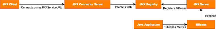
JMX monitoring steps include:
- The Java application acting as the JMX server creates and configures MBeans for the desired metrics.
- JMX server registers the MBeans with the JMX registry.
- JMXConnectorServerFactory creates the JMXConnectorServer that defines the JMXServiceURL that provides the entry point details for the JMX client.
- JMXClient connects to the JMX registry in the JMX server using the JMXServiceURL and the JMXConnectorServer.
- The JMX server handles client requests, interacting with the JMX registry to retrieve the MBean data.
Solution overview
This method of wrapping supported Kafka connectors with custom code that exposes connector-specific operational metrics enables teams to get better insights by correlating various connector metrics with cloud-centered metrics in monitoring systems such as Amazon CloudWatch. This approach enables consistent monitoring across different components of the change data capture (CDC) pipeline, ultimately feeding metrics into unified dashboards while respecting each connector’s architectural philosophy. The consolidated metrics can be delivered to CloudWatch or the monitoring tool of your choice including partner specific application performance management (APM) tools such as Datadog, New Relic, and so on.
We have the working implementation of this same approach with two popular connectors: Debezium source connector and MongoDB Sink Connector. You can find the Github sample and ready to use plugins built for each in the repository. Review the README file for this custom implementation for more details.
For example, our custom implementation for the MongoDB Sink Connector adds a metrics export layer that calculates critical performance indicators such as latest-kafka-time-difference-ms – which measures the latency between Kafka message timestamps and connector processing time by subtracting the connector’s current clock time from the last received record’s timestamp. This custom wrapper around the MongoDB Sink Connector enables exporting relevant JMX metrics and publishing them as custom metrics to CloudWatch. We’ve open sourced this solution on GitHub, along with a ready-to-use plugin and detailed configuration guidance in the README.
CDC is the process of identifying and capturing changes made in a database and delivering those changes in real time to a downstream system. Debezium is an open source distributed platform built on top of Apache Kafka that provides CDC functionality. It provides a set of connectors to track and stream changes from databases to Kafka.
In the next section, we dive deep into the implementation details of how to export JMX metrics from Debezium MySQL Connector deployed as a custom plugin in Amazon MSK Connect. The connector plugin takes care of creating and configuring the MBeans and registering them with the JMX registry.
The following diagram shows the workflow of using Debezium MySQL Connector as a custom plugin in Amazon MSK Connect for CDC from an Amazon Aurora MySQL-Compatible Edition data source.
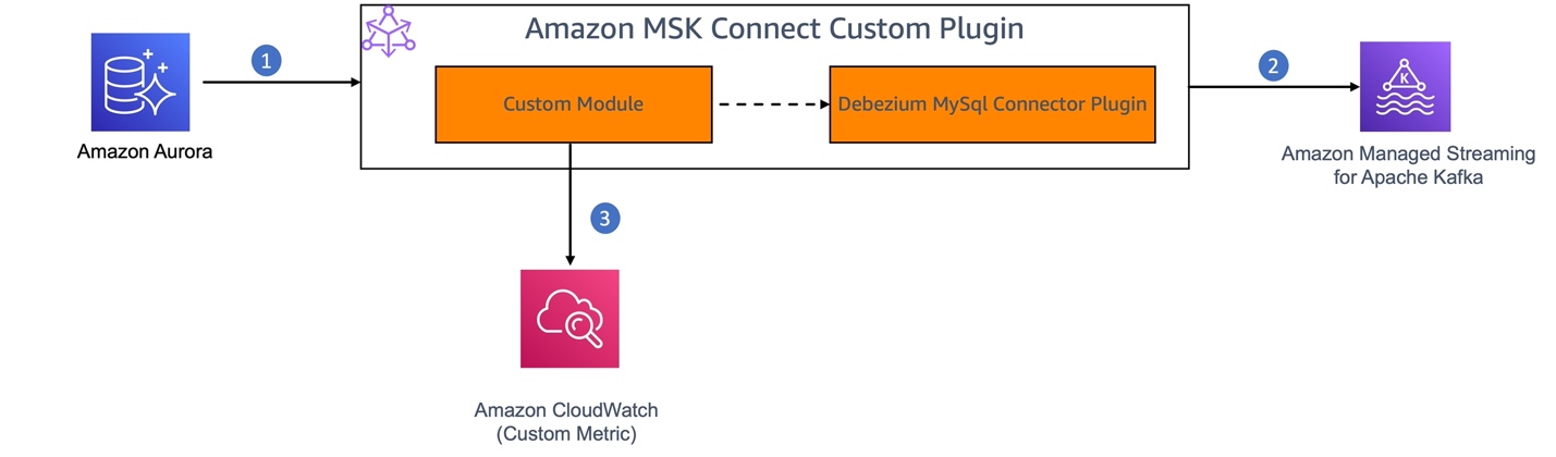
- MySQL binary log (binlog) is enabled in Amazon Aurora for MySQL to record all the operations in the order in which they are committed to the database.
- The Debezium connector plugin component of the MSK Connect custom plugin continuously monitors the MySQL database, captures the row-level changes by reading the MySQL bin logs, and streams them as change events to Kafka topics in Amazon MSK.
- We’ll build a custom module to enable JMX monitoring on the Debezium connector. This module will act as a JMX client to retrieve the JMX metrics from the connector and publish them as custom metrics to CloudWatch.
The Debezium connector provides three types of metrics in addition to the built-in support for default Kafka and Kafka Connect JMX metrics.
- Snapshot metrics provide information about connector operation while performing a snapshot.
- Streaming metrics provide information about connector operation when the connector is reading the binlog.
- Schema history metrics provide information about the status of the connector’s schema history.
In this solution, we export the MilliSecondsBehindSource streaming metrics emitted by the Debezium MySQL connector. This metric provides the number of milliseconds that the connector is lagging behind the change events in the database.
Prerequisites
Following are the prerequisites you need:
- Access to the AWS account where you want to set up this solution.
- You have set up the source database and MSK cluster by following this setup instructions in the MSK Connect workshop.
Create a custom plugin
Creating a custom plugin for Amazon MSK Connect for the solution involves the following steps:
- Create a custom module: Create a new Maven module or project that will contain your custom code to:
- Enable JMX monitoring in the connector application by starting the JMX server.
- Create a Remote Method Invocation (RMI) registry to enable the access to the JMX metrics to the clients.
- Create a JMX metrics exporter to query the JMX metrics by connecting to the JMX server and push the metrics to CloudWatch as custom metrics.
- Schedule to run the JMX metrics exporter at a configured interval.
- Package and deploy the custom module as an MSK Connect custom plugin.
- Create a connector using the custom plugin to capture CDC from the source, stream it and validate the metrics in Amazon CloudWatch.
This custom module extends the connector functionality to export the JMX metrics without requiring any changes in the underlying connector implementation. This helps ensure that upgrading the custom plugin requires only upgrading the plugin version in the pom.xml of the custom module.
Let’s deep dive and understand the implementation of each step mentioned above.
1. Create a custom module
Create a new Maven project with dependencies on Debezium MySQL Connector to enable JMX monitoring, Kafka Connect API for configuration, and CloudWatch AWS SDK to push the metrics to CloudWatch.
Set up a JMX connector server to enable JMX monitoring: To enable JMX monitoring, the JMX server needs to be started at the time of initializing the connector. This is usually done by setting the environment variables with JMX options as described in Monitoring Debezium. In the case of an Amazon MSK Connect custom plugin, JMX monitoring is enabled programmatically at the time of connector plugin initialization. To achieve this:
- Extend the
MySqlConnectorclass and override thestartwhich is the connector’s entry point to execute custom code.
- In the
startmethod of the custom connector class (DebeziumMySqlMetricsConnector) that we are creating, set the following parameters to allow customization of the JMX Server properties by retrieving connector configuration from a config file.
connect.jmx.port – The port number on which the RMI registry needs to be created. JMXConnectorServer would listen to the incoming connections on this port.
database.server.name – Name of the database that is the source for the CDC.
It also retrieves the CloudWatch configuration related properties that will be used while pushing the JMX metrics to CloudWatch.
cloudwatch.namespace.name – CloudWatch NameSpace to which the metrics need to be pushed as custom metrics
cloudwatch.region – CloudWatch Region where the custom namespace is created in your AWS account
- Create an RMI registry on the specified port (
connectJMXPort). This registry is used by the JMXConnectorServer to store the RMI objects corresponding to the MBeans in the JMX registry. This allows the JMX clients to look up and access the MBeans on the PlatformMBeanServer.
LocateRegistry.createRegistry(connectJMXPort);
- Retrieve the
PlatformMBeanServerand construct theJMXServiceURLwhich is in the formatservice:jmx:rmi://localhost/jndi/rmi://localhost:<<jmx.port>>/jmxrmi. Create a new JMXConnectorServer instance using the JMXConnectorServerFactory and the JMXServiceURL and start the JMXConnectorServer instance.
Implement JMX metrics exporter: Create a JMX client to connect to the JMX server, query the MilliSecondBehindSource metric from the JMX server, convert it into the required format, and export it to CloudWatch.
- Connect to the JMX Server using the
JMXConnectorFactoryandJMXServiceURL
- Query the MBean object that holds the corresponding metric, for example,
MilliSecondsBehindSource, and retrieve the metric value using sample code provided in msk-connect-custom-plugin-jmx. (you can choose one or more metrics). - Schedule the execution of your JMX metrics exporter at regular intervals.
getScheduler().schedule(new JMXMetricsExporter(), SCHEDULER_INITIAL_DELAY, SCHEDULER_PERIOD);
Export metrics to CloudWatch: Implement the logic to push relevant JMX metrics to CloudWatch. You can use the AWS SDK for Java to interact with the CloudWatch PutMetricData API or use the CloudWatch Logs subscription filter to ingest the metrics from a dedicated Kafka topic.
For more information, see the sample implementation for the custom module in aws-samples in GitHub. This sample also provides custom plugins packaged with two different versions of Debezium MySQL connector (debezium-connector-mysql-2.5.2.Final-plugin and debezium-connector-mysql-2.7.3.Final-plugin) and the following steps would explain the steps to build a custom plugin using your custom code.
2. Package the custom module and Debezium MySQL connector as a custom plugin
Build and package the Maven project with the custom code as a JAR file and include the JAR file in the debezium-connector-mysql-2.5.2.Final-plugin folder downloaded from maven repo. Package the updated debezium-connector-mysql-2.5.2.Final-plugin as a ZIP file (Amazon MSK Connect accepts custom plugins in ZIP or JAR format). Alternatively, you can use the prebuiltcustom-debezium-mysql-connector-plugin.zip available in GitHub.
Choose the Debezium connector version (2.5 or 2.7) that fits your requirement.
When you have to upgrade to a new version of the Debezium MySQL connector, you can update the version of the dependency and build the custom module and deploy it. By doing this, you can maintain the custom plugin without modifying the original connector code. The GitHub samples provide ready-to-use plugins for two Debezium connector versions. However, you can follow the same approach to upgrade to the latest connector version as well.
Create a custom plugin in Amazon MSK
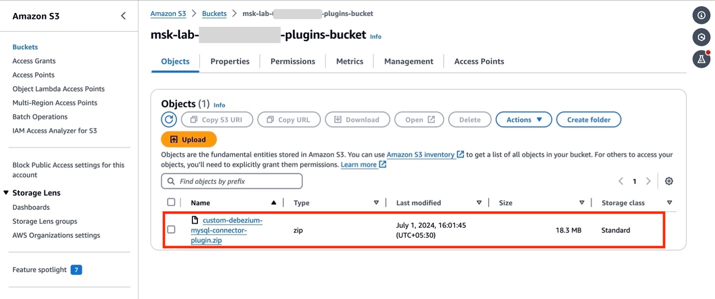
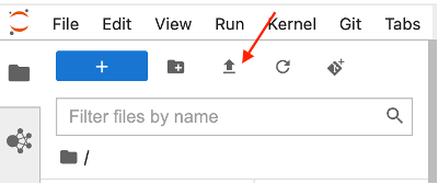
- If you have set up your AWS resources by following the Getting Started lab, open Amazon S3 console and locate the bucket
msk-lab-${ACCOUNT_ID}-plugins-bucket/debezium. - Upload the custom plugin created in the previous section
custom-debezium-mysql-connector-plugin.ziptomsk-lab-${ACCOUNT_ID}-plugins-bucket/debezium, as shown in the following figure.
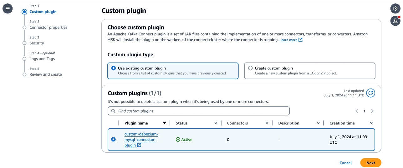
- Switch to the Amazon MSK console and choose Custom plugins in the navigation pane. Choose Create custom plugin and, browse the S3 bucket that you created above and select the custom plugin ZIP file you just uploaded.
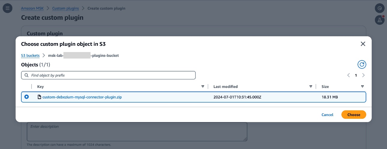
- Enter
custom-debezium-mysql-connector-pluginfor the plugin name. Optionally, enter a description and choose Create Custom Plugin.
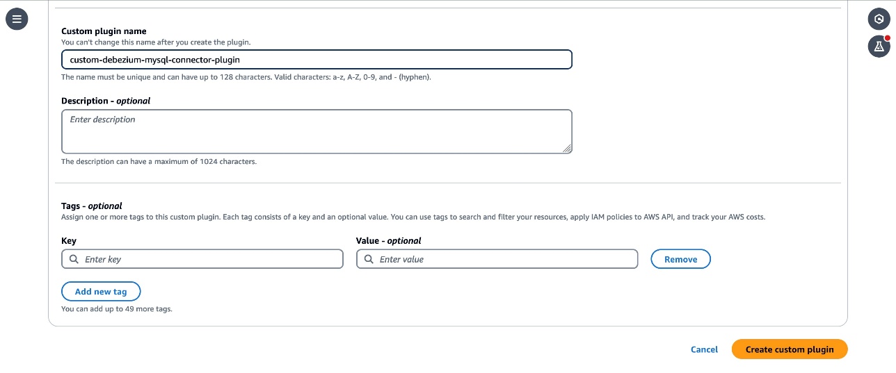
- After a few seconds you should see the plugin is created and the status is
Active. - Customize the worker configuration for the connector by following the instructions in the Customize worker configuration lab.
3. Create an Amazon MSK connector
The next step is to create an MSK connector.
- From the MSK section choose Connectors, then choose Create connector. Choose
custom-debezium-mysql-connector-pluginfrom the list of Custom plugins, then choose Next.
- Enter
custom-debezium-mysql-connectorin the Name textbox, and a description for the connector.
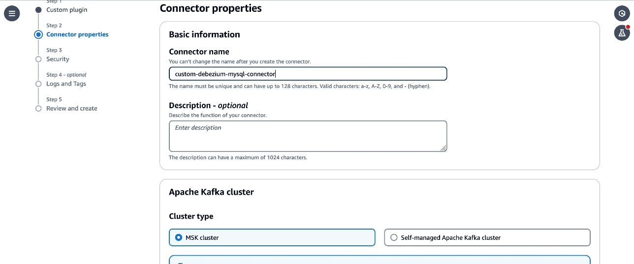
- Select the
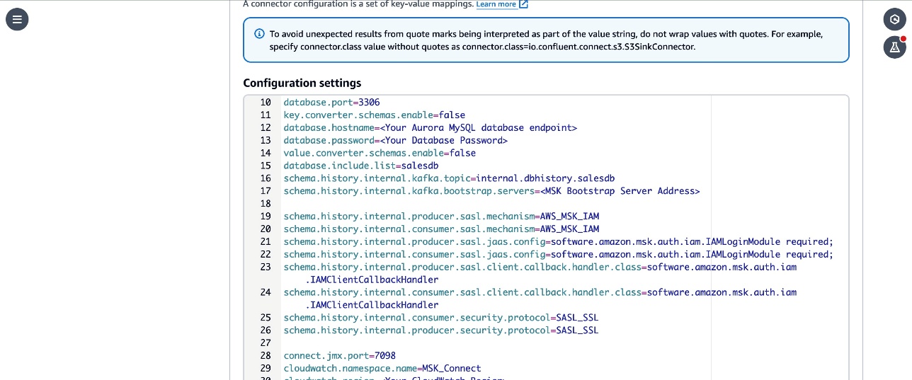
MSKCluster-msk-connect-labfrom the listed MSK clusters. From the Authentication dropdown, select IAM. - Copy the following configuration and paste it in the connector configuration textbox.
- Replace the
<Your Aurora MySQL database endpoint>,<Your Database Password>,<Your MSK Bootstrap Server Address>, and<Your CloudWatch Region>placeholders with the corresponding details for the resources in your account. - Review the
topic.prefix,database.user,topic.prefix,database.server.id,database.server.name,database.port,database.include.listparameters in the configuration. These parameters are configured with the values used in the workshop. Update them with the details corresponding to your configuration if you have customized it in your account. - Note that the
connector.classparameter is updated with the qualified name of the subclass of MySqlConnector class that you created in the custom module. - The
connect.jmx.portparameter specifies the default port to start the JMX server. You can configure this to any available port.
5. Follow the remaining instructions from the Create MSK Connector lab and create the connector. Verify that the connector status changes to Running.
Debezium MySQL custom connector version (2.7.3) provides additional flexibility to configure optional properties that can be added to your MSK connector configuration and selectively include and exclude metrics to emit to CloudWatch. The following are the example configuration properties that can be used with version 2.7.3 :
- cloudwatch.debezium.streaming.metrics.include – A comma-separated list of streaming metrics type that must be exported to CloudWatch as custom metrics.
- cloudwatch.debezium.streaming.metrics.exclude – Specify a comma-separated list of streaming metrics types to exclude from being sent to CloudWatch as custom metrics.
- Similarly include and exclude properties for snapshot metrics type are cloudwatch.debezium.snapshot.metrics.include and cloudwatch.debezium.snapshot.metrics.exclude
- Include and exclude properties for schema history metrics type are cloudwatch.debezium.schema.history.metrics.include and cloudwatch.debezium.schema.history.metrics.exclude
The following is a sample configuration excerpt.
Review the GitHub README file for more details on the use of these properties with MSK connector configurations.
Verify the replication in the Kafka cluster and CloudWatch metrics
Follow the instructions in the Verify the replication in the Kafka cluster lab to set up a client and make changes to the source DB and verify that the changes are captured and sent to Kafka topics by the connector.
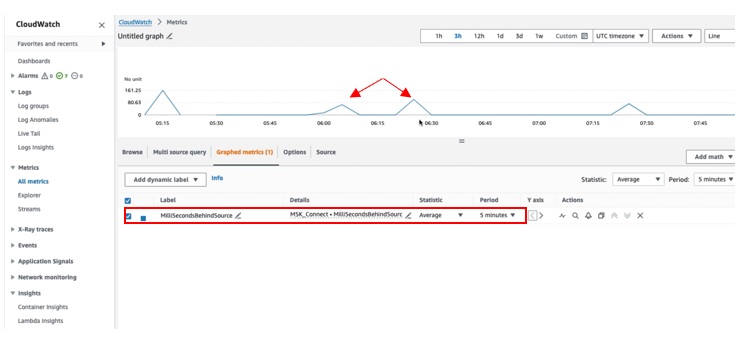
To verify that the connector has published the JMX metrics to CloudWatch, go to the CloudWatch console and choose Metrics in the navigation pane, then choose All Metrics. Under Custom namespace, you can see MSK_Connect with database name as the dimension. Select the database name to view the metrics.
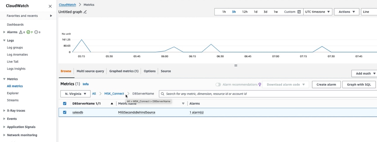
Select the MilliSecondBehindSource metric with statistic as Average in the Graphed Metric to plot the graph. You can verify that the MilliSecondBehindSource metric value is greater than zero whenever any operation is being performed on the source database and returns to zero during the idle time.
Clean up
Delete the resources that you created such as the Aurora DB, Amazon MSK Cluster and connectors by following the instructions at Cleanup in the Amazon MSK Connect lab if you have been following along to set up the solution on your account.
Conclusion
In this post, we showed you how to extend the Debezium MySQL connector plugin with an additional module to export the JMX metrics to CloudWatch as custom metrics. As a next step, you can create a CloudWatch alarm to monitor the metrics and take remediation actions when the alarm is triggered. In addition to exporting the JMX metrics to CloudWatch, you can export these metrics to third-party applications such as Prometheus or DataDog using CloudWatch Metric Streams. You can follow a similar approach to export the JMX metrics of other connectors from MSK Connect. You can learn more about creating your own connectors by visiting the Connector Developer Guide and how to deploy them as custom plugins in the MSK Connect documentation.
About the authors
 Jaydev Nath is a Solutions Architect at AWS, where he works with ISV customers to build secure, scalable, reliable, and cost-efficient cloud solutions. He brings strong expertise in building SaaS architecture on AWS with a focus on Generative AI and data analytics technologies to help deliver practical, valuable business outcomes for customers.
 David John Chakram is a Principal Solutions Architect at AWS. He specializes in building data platforms and architecting seamless data ecosystems. With a profound passion for databases, data analytics, and machine learning, he excels at transforming complex data challenges into innovative solutions and driving businesses forward with data-driven insights.
 Sharmila Shanmugam is a Solutions Architect at Amazon Web Services. She is passionate about solving the customers’ business challenges with technology and automation and reduce the operational overhead. In her current role, she helps customers across industries in their digital transformation journey and build secure, scalable, performant and optimized workloads on AWS.

 Venkatavaradhan (Venkat) Viswanathan is a Global Partner Solutions Architect at Amazon Web Services. Venkat is a Technology Strategy Leader in Data, AI, ML, generative AI, and Advanced Analytics. Venkat is a Global SME for Databricks and helps AWS customers design, build, secure, and optimize Databricks workloads on AWS.
 Srividya Parthasarathy is a Senior Big Data Architect on the AWS Lake Formation team. She works with the product team and customers to build robust features and solutions for their analytical data platform. She enjoys building data mesh solutions and sharing them with the community.
 Ramkumar Nottath is a Principal Solutions Architect at AWS focusing on Analytics services. He enjoys working with various customers to help them build scalable, reliable big data and analytics solutions. His interests extend to various technologies such as analytics, data warehousing, streaming, data governance, and machine learning. He loves spending time with his family and friends.
 John Spencer is a Product Manager at Databricks, dedicated to making Unity Catalog work seamlessly with customers’ ecosystems of tools and platforms so they can easily access, govern, and use their data.
 Sreeram Thoom is a Specialist Solutions Architect at Databricks helping customers design secure, scalable applications on the Data Lakehouse.
 Dipankar Kushari is a specialist solutions architect at Databricks helping customer architect and build secured applications on Data Lakehouse.


 Aarthi Srinivasan is a Senior Big Data Architect with AWS Lake Formation. She collaborates with the service team to enhance product features, works with AWS customers and partners to architect lake house solutions, and establishes best practices.
 Parul Saxena is a Senior Big Data Specialist Solutions Architect in AWS. She helps customers and partners build highly optimized, scalable, and secure solutions. She specializes in Amazon EMR, Amazon Athena, and AWS Lake Formation, providing architectural guidance for complex big data workloads and assisting organizations in modernizing their architectures and migrating analytics workloads to AWS.


 Asser Moustafa is a Principal Worldwide Specialist Solutions Architect at AWS, based in Dallas, Texas, USA. He partners with customers worldwide, advising them on all aspects of their data architectures, migrations, and strategic data visions to help organizations adopt cloud-based solutions, maximize the value of their data assets, modernize legacy infrastructures, and implement cutting-edge capabilities like machine learning and advanced analytics. Prior to joining AWS, Asser held various data and analytics leadership roles, completing an MBA from New York University and an MS in Computer Science from Columbia University in New York. He is passionate about empowering organizations to become truly data-driven and unlock the transformative potential of their data.
 Pinar Yasar is the Data Engineering Manager at Getir. Her passion is to accelerate self-service analytics for her internal customers and build highly scalable and cost-effective solutions in the cloud.


 Ritesh Kumar Sinha is an Analytics Specialist Solutions Architect based out of San Francisco. He has helped customers build scalable data warehousing and big data solutions for over 16 years. He loves to design and build efficient end-to-end solutions on AWS. In his spare time, he loves reading, walking, and doing yoga.
 Tahir Aziz is an Analytics Solution Architect at AWS. He has worked with building data warehouses and big data solutions for over 15+ years. He loves to help customers design end-to-end analytics solutions on AWS. Outside of work, he enjoys traveling and cooking.
 Omama Khurshid is an Acceleration Lab Solutions Architect at Amazon Web Services. She focuses on helping customers across various industries build reliable, scalable, and efficient solutions. Outside of work, she enjoys spending time with her family, watching movies, listening to music, and learning new technologies.


 Salim Tutuncu is a Sr. PSA Specialist on Data & AI, based from Amsterdam with a focus on the EMEA North and EMEA Central regions. With a rich background in the technology sector that spans roles as a Data Engineer, Data Scientist, and Machine Learning Engineer, Salim has built a formidable expertise in navigating the complex landscape of data and artificial intelligence. His current role involves working closely with partners to develop long-term, profitable businesses leveraging the AWS Platform, particularly in Data and AI use cases.
 Angel Conde Manjon is a Sr. PSA Specialist on Data & AI, based in Madrid, and focuses on EMEA South and Israel. He has previously worked on research related to Data Analytics and Artificial Intelligence in diverse European research projects. In his current role, Angel helps partners develop businesses centered on Data and AI.
 Mukul Sharma is a Software Development Engineer on Data & Analytics (DnA) organization at GoDaddy. He is a polyglot programmer with experience in a wide array of technologies to rapidly deliver scalable solutions. He enjoys singing karaoke, playing various board games, and working on personal programming projects in his spare time.
 Ozcan Ilikhan is a Director of Engineering on Data & Analytics (DnA) organization at GoDaddy. He is passionate about solving customer problems and increasing efficiency using data and ML/AI. In his spare time, he loves reading, hiking, gardening, and working on DIY projects.
 Harsh Vardhan Singh Gaur is an AWS Solutions Architect, specializing in analytics. He has over 6 years of experience working in the field of big data and data science. He is passionate about helping customers adopt best practices and discover insights from their data.
 Ramesh Kumar Venkatraman is a Senior Solutions Architect at AWS who is passionate about containers and databases. He works with AWS customers to design, deploy, and manage their AWS workloads and architectures. In his spare time, he loves to play with his two kids and follows cricket.


 Tom Romano is a Sr. Solutions Architect for AWS World Wide Public Sector from Tampa, FL, and assists GovTech and EdTech customers as they create new solutions that are cloud native, event driven, and serverless. He is an enthusiastic Python programmer for both application development and data analytics, and is an Analytics Specialist. In his free time, Tom flies remote control model airplanes and enjoys vacationing with his family around Florida and the Caribbean.
 Shane Thompson is a Sr. Solutions Architect based out of San Luis Obispo, California, working with AWS Startups. He works with customers who use AI/ML in their business model and is passionate about democratizing AI/ML so that all customers can benefit from it. In his free time, Shane loves to spend time with his family and travel around the world.
 Sindhu Chandra is a Senior Product Marketing Manager for Amazon QuickSight, AWS’ cloud-native, business intelligence (BI) service that delivers easy-to-understand insights to anyone, wherever they are.


 Chao Pan is a Data Analytics Solutions Architect at Amazon Web Services. He’s responsible for the consultation and design of customers’ big data solution architectures. He has extensive experience in open-source big data. Outside of work, he enjoys hiking.


 Varad Ram is Senior Solutions Architect in Amazon Web Services. He likes to help customers adopt to cloud technologies and is particularly interested in artificial intelligence. He believes deep learning will power future technology growth. In his spare time, he like to be outdoor with his daughter and son.


 Changbin Gong is a Senior Solutions Architect at Amazon Web Services (AWS). He engages with customers to create innovative solutions that address customer business problems and accelerate the adoption of AWS services. In his spare time, Changbin enjoys reading, running, and traveling.


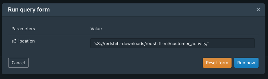
 You would probably like to reuse the load query in the future to load data in from another S3 location. In that case, you can use the parameterized query by replacing the S3 URL of the as shown in the following screenshot:


 Debu Panda is a Principal Product Manager at AWS, is an industry leader in analytics, application platform, and database technologies, and has more than 25 years of experience in the IT world.
 Cansu Aksu is a Front End Engineer at AWS, has a several years of experience in developing user interfaces. She is detail oriented, eager to learn and passionate about delivering products and features that solve customer needs and problems
 Chengyang Wang is a Frontend Engineer in Redshift Console Team. He worked on a number of new features delivered by redshift in the past 2 years. He thrives to deliver high quality products and aim to improve customer experience from UI
