Post Syndicated from xkcd.com original https://xkcd.com/3283/
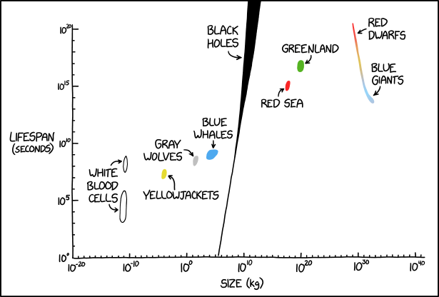
Post Syndicated from xkcd.com original https://xkcd.com/3283/
Post Syndicated from corbet original https://lwn.net/Articles/1087961/
The 7.2-rc7 kernel prepatch is out for
testing. It is still bigger than Linus would like, but he said
nonetheless: “I don’t currently see any value in delaying the 7.2
“
release, so I would expect that to happen next weekend unless something
really bad pops up.
Post Syndicated from Rohit Kumar original https://www.servethehome.com/wisdpi-wp-ut9-usb-10gbe-adapter-realtek-rtl8159-review/
We check out the WisdPi WP-UT9, which is a stylish USB Type-C external 10Gbase-T adapter based on the Realtek RTL8159 10GbE platform
The post WisdPi WP-UT9 USB 10GbE Adapter Review appeared first on ServeTheHome.
Post Syndicated from LastWeekTonight original https://www.youtube.com/watch?v=sYYuW9YJshU
Post Syndicated from Explosm.net original https://explosm.net/comics/children
New Cyanide and Happiness Comic
Post Syndicated from Oglaf! -- Comics. Often dirty. original https://www.oglaf.com/risk/


Post Syndicated from LastWeekTonight original https://www.youtube.com/watch?v=1BqWBJmLyy8
Post Syndicated from Ryan Smith original https://www.servethehome.com/deltas-gocool-150-goes-big-to-enable-150kw-liquid-to-air-cooling-for-asrock-racks-vr-nvl72/
How do you cool a giant rack of AI hardware? With an even bigger heat exchanger. Delta’s GoCool-150 is a liquid-to-air CDU that is designed to dissipate 150kW of heat from NVL72 and other high-density liquid cooled racks
The post Delta’s GoCool-150 Goes Big To Enable 150kW Liquid-To-Air Cooling for ASRock Rack’s NVIDIA VR NVL72 appeared first on ServeTheHome.
Post Syndicated from The Atlantic original https://www.youtube.com/shorts/P6yofim8i80
Post Syndicated from Techmoan original https://www.youtube.com/watch?v=nY4ZbIxbvIU
Post Syndicated from The Atlantic original https://www.youtube.com/shorts/QSsntklkhkk
Post Syndicated from Bruce Schneier original https://www.schneier.com/blog/archives/2026/08/friday-squid-blogging-arctic-bobtail-squid-video.html
Nice video of the Arctic bobtail squid.
As usual, you can also use this squid post to talk about the security stories in the news that I haven’t covered.
Post Syndicated from Vladimir Provorov original https://aws.amazon.com/blogs/security/a-decade-of-enterprise-identity-in-the-cloud-with-aws-managed-microsoft-ad/
Ten years ago, we launched AWS Directory Service for Microsoft Active Directory, a fully managed Microsoft Active Directory in the AWS Cloud. In that original announcement, Jeff Barr described a straightforward promise: “You will spend less time administering and more time working on your applications and your business.”
A decade later, AWS Managed Microsoft AD has become the identity backbone for thousands of enterprises worldwide. What started as a way to run directory-aware workloads in the cloud now powers SQL Server authentication, Amazon WorkSpaces virtual desktops, and Amazon FSx for Windows File Server for thousands of enterprises worldwide.
In 2015, customers migrating Windows workloads to Amazon Web Services (AWS) faced a familiar challenge. Microsoft Active Directory (AD) had become the dominant standard for enterprise identity, by some estimates commanding 90% market share for directory services in the Fortune 1000. Running SharePoint, SQL Server, .NET applications, or virtually any Windows workload meant running AD.
However, running AD well comes with significant operational overhead. It requires careful capacity planning, high availability design across multiple sites, ongoing patching and maintenance, backup and disaster recovery procedures, and deep expertise that’s increasingly difficult to find and retain. Customers told us they wanted to focus on their applications, not on managing domain controllers.
So we built AWS Managed Microsoft AD. Powered by actual Windows Server, it delivered real Microsoft AD (not a compatible alternative, but the genuine article) as a fully managed service. We handled the domain controller deployment, the multi-AZ high availability, the automated backups, the patching, the monitoring, and many more features including scalability and multi-Region replication. Customers got a directory they could provision in 25–30 minutes and start using immediately.
From that original What’s New announcement by Bryan Nairn:
“AWS Directory Service now lets you run a Microsoft Active Directory (AD) as a managed service… Host monitoring and recovery, data replication, snapshots, and software updates are automatically configured and managed for you.”
Looking back at the past 10 years, we’re struck by how much AWS Managed Microsoft AD has evolved in response to customer feedback. Here are some of the highlights:
2015: Launch of AWS Managed Microsoft AD (Enterprise Edition) in five AWS Regions, powered by Windows Server 2012 R2. Support for trust relationships with on-premises AD, seamless domain join for Amazon Elastic Compute Cloud (Amazon EC2) instances, and integration with Amazon WorkSpaces.
2017: Introduction of Standard Edition, optimized for small and midsize businesses. This gave customers a cost-effective option for resource forest deployments and smaller workloads.
2018: Added support for schema extensions, enabling customers to extend their directory schema for applications that require custom attributes. Support for Group Managed Service Accounts (gMSA) with Windows containers and other services.
2019: Launched multi-Region replication for Enterprise Edition, allowing customers to automatically replicate their directory across AWS Regions for improved performance and disaster recovery. Added directory sharing across AWS accounts and integration with AWS Organizations.
2020: Introduced fine-grained directory settings for security and compliance, enabling customers to configure secure channel settings for protocols and ciphers. Enhanced compliance support—with the service now HIPAA eligible—included as an in-scope service under PCI DSS, and achieving FedRAMP authorization.
2021: Added CloudWatch metrics for domain controllers, helping customers optimize scaling decisions based on CPU, memory, disk, and AD-specific metrics like DNS and directory read/write operations. Launched integration with AWS Transfer Family for SFTP/FTPS/FTP authentication.
2022: Windows Server 2019 upgrade became available, with customer-initiated updates and automatic migration for all directories beginning in 2023.
2023: AWS Private CA Connector for Active Directory launched, allowing customers to replace self-managed enterprise certificate authorities with AWS Private CA for automatic certificate enrollment to domain-joined objects, with no local agents or proxy servers required.
2024: Launched CRUD APIs for users and groups, enabling IT administrators to manage AD users and groups directly from the AWS Management Console, AWS Command Line Interface (AWS CLI), and APIs, without deploying bastion hosts or opening network ports.
2025: General availability of AWS Managed Microsoft AD (Hybrid Edition), allowing customers to extend their existing AD domain to AWS while retaining administrative control. Introduced self-service edition upgrades through the UpdateDirectorySetup API, eliminating the need for support tickets when scaling from Standard to Enterprise Edition.
2026 and beyond: As we enter our second decade, our roadmap continues to be shaped by the customers who depend on AWS Managed Microsoft AD every day. We’re working on new capabilities driven directly by your feedback, and we look forward to sharing more soon.
Over the past decade, more than 20 AWS services have added native integration with AWS Managed Microsoft AD. What started with WorkSpaces and EC2 domain join has expanded to more than 20 AWS services, making AWS Managed Microsoft AD foundational for many enterprise customers’ workloads on AWS.
For many customers, database authentication is a primary driver for adopting AWS Managed Microsoft AD. By pairing Amazon Relational Database Service (Amazon RDS) for SQL Server with AWS Managed Microsoft AD, they gain the benefits of fully managed services while achieving straightforward integration and reduced management overhead. This combination lets developers and DBAs use their existing AD credentials to access SQL Server databases, so they don’t need to manage separate database accounts.
Beyond SQL Server, AWS Managed Microsoft AD enables Windows authentication across the Amazon RDS family:
Amazon FSx for Windows File Server provides fully managed Windows file shares that integrate natively with AWS Managed Microsoft AD. Customers use AD users and groups to control access to file shares, apply Windows ACLs, and use features like DFS namespaces, all with the same management experience they use on premises.
AWS Storage Gateway supports AD authentication for SMB file shares, enabling hybrid storage architectures where on-premises applications access cloud storage using familiar AD credentials.
AWS Transfer Family added AD integration in 2021, allowing customers to authenticate SFTP, FTPS, and FTP users against their AWS Managed Microsoft AD. This allows customers to migrate file transfer workflows without changing end-user credentials.
Amazon end-user computing services were among the first to integrate with AWS Managed Microsoft AD:
AWS IAM Identity Center (formerly AWS Single Sign-On) uses AWS Managed Microsoft AD as an identity source, synchronizing users and groups to provide single sign-on access across AWS accounts and applications. This provides centralized identity management while using your existing AD infrastructure.
AWS Client VPN authenticates users against AWS Managed Microsoft AD, providing secure remote access using corporate credentials.
AWS Management Console access can be federated through AWS Managed Microsoft AD, so AD users can assume AWS Identity and Access Management (IAM) roles and manage AWS resources with their existing credentials.
Amazon EC2 instances (both Windows and Linux) support seamless domain join at launch. Windows instances can be managed using Group Policy, and Linux instances can authenticate users through SSSD or Realm integration.
Amazon Elastic Container Service (Amazon ECS) supports AD authentication for Windows containers through Group Managed Service Accounts (gMSA), enabling containerized applications to authenticate to AD-integrated resources.
This breadth of integration means customers can standardize on a single directory for their entire AWS environment, from databases to desktops to file servers to analytics.
Over the years, we’ve learned that customers have different needs when it comes to managed AD. Today, AWS Managed Microsoft AD is available in three editions, each designed for specific use cases.
Standard Edition is optimized for small and midsize businesses, or for enterprises deploying a resource forest model in a single AWS Region. With 1 GB of directory object storage supporting up to 30,000 objects (approximately 5,000 users), Standard Edition provides everything needed to run directory-aware workloads without the overhead of managing domain controllers.
Common use cases:
Standard Edition is a great starting point, and customers aren’t locked in. With our new self-service upgrade capability (launched October 2025), you can upgrade to Enterprise Edition programmatically through the UpdateDirectorySetup API, no support tickets or maintenance window coordination required.
Enterprise Edition is designed for organizations with larger user populations, complex deployments, or global footprints. With 17 GB of storage supporting up to 500,000 directory objects, Enterprise Edition provides the capacity and capabilities that large enterprises require.
Key capabilities:
If you have users and applications in multiple geographic regions, or anticipate significant growth in directory objects, Enterprise Edition is the right choice.
Launched earlier this year, Hybrid Edition takes a fundamentally different approach. Instead of creating a new AD domain in AWS, Hybrid Edition extends your existing AD domain into the cloud.
What makes Hybrid Edition unique:
Hybrid Edition is ideal for customers who want the operational benefits of AWS-managed domain controller infrastructure without changing their AD architecture or giving up administrative control.
Use the following table to determine which edition best fits your use case.
| Use case | Edition |
| A new AD domain for AWS workloads in a single Region | Standard Edition |
| A resource forest with trust to on-premises AD | Standard Edition |
| Multi-Region replication for global deployments | Enterprise Edition |
| Support for more than 30,000 directory objects | Enterprise Edition |
| To extend your existing AD domain to AWS | Hybrid Edition |
| To retain full administrative control over your AD | Hybrid Edition |
Looking back at the decisions we made in 2015, several have proven foundational to the service’s success:
As we celebrate 10 years of AWS Managed Microsoft AD, we’re excited about what’s ahead. The launch of Hybrid Edition earlier this year represents a significant expansion of what’s possible, giving customers new flexibility in how they architect their identity infrastructure for hybrid and multi-cloud environments.
We continue to listen to customer feedback and invest in capabilities that reduce operational burden while expanding what you can build. Whether you’re running your first SQL Server database in the cloud, deploying virtual desktops to a global workforce, or modernizing legacy applications that depend on AD, AWS Managed Microsoft AD is here to help.
Thank you to all the customers who have trusted us with their identity infrastructure over the past decade. Your feedback has shaped this service, and we’re committed to continuing to earn that trust for the next 10 years and beyond.
Ready to get started or learn more? Here are some resources:
If you have feedback about this post, submit comments in the Comments section below.
Post Syndicated from Sam Sabinash original https://www.servethehome.com/a-10m-iops-kioxia-gp1-ssd-shown-running-at-fms-2026/
At FMS 2026, we saw the Kioxia GP1 PCIe Gen6 NVMe SSD running live in the company’s booth at just over 10M IOPS
The post A 10M IOPS Kioxia GP1 SSD Shown Running at FMS 2026 appeared first on ServeTheHome.
Post Syndicated from Hetal Kolekar original https://aws.amazon.com/blogs/security/securing-your-amazon-s3-buckets-identifying-and-remediating-over-permissioned-access/
Misconfigured Amazon Simple Storage Service (Amazon S3) buckets can expose your data to unauthorized access. Without proactive review, S3 bucket policies or Access Control Lists (ACLs) configured with broad access may go unnoticed in your environment. In this post, you learn how to identify and fix over-permissioned S3 buckets across your AWS environment, along with best practice recommendations and automation opportunities to help you prevent security gaps. This post provides a workflow framework and methodology recommendations for your security team to adapt. The focus of this post is on the what and why rather than a prescriptive implementation. You will need to customize the approach based on your organization’s requirements and existing security tooling.
This solution is intended for security engineers, cloud architects, and DevOps teams managing single- or multiple-account AWS environments with Amazon S3 workloads that require access management.
Before you begin, make sure you have the following in place:
This solution uses a five-phase workflow diagram to detect, remediate, and continuously monitor over-permissioned S3 buckets across your AWS accounts. The following workflow diagram illustrates the high-level end-to-end process for identifying and remediating over-permissioned S3 buckets across your Amazon Web Services (AWS) environment.
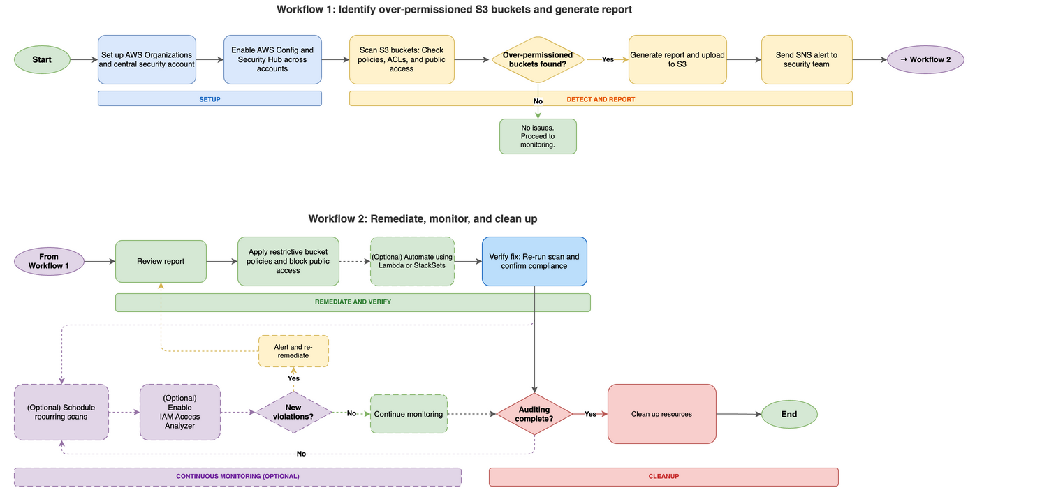
Figure 1: Amazon S3 over-permissive access – Detection, remediation, monitoring and cleanup workflow
The diagram in Figure 1 consists of five phases:
This section covers the AWS services used in this solution and their associated costs so you can estimate spend before deployment. The primary cost drivers are AWS Config and Security Hub, which scale with the number of accounts and resources you monitor. Lambda, Amazon EventBridge, Amazon SNS, and Amazon S3 typically add minimal costs for most environments. Start with a pilot in one or two accounts to validate costs before scaling.
Check the service pricing pages for current rates. Use the AWS Pricing Calculator to estimate costs for your specific environment before enabling services across all accounts. Consider starting with a pilot in one or two accounts to validate costs before scaling.
This section walks you through setting up the audit environment, deploying the Lambda-based scanner, and generating reports of over-permissioned S3 buckets across your accounts. Follow these steps to identify over-permissioned S3 buckets in your multi-account environment, starting with preparing your environment for an Amazon S3 audit.
To set up the multi-account audit environment:
Note: The specific trust policy and permissions policy for your cross-account roles will depend on organizational requirements. Work with your IAM administrators to grant minimum necessary access for the audit function.
sts:AssumeRolepermission for the cross-account role ARNs created in step 5. The AWS Lambda execution role documentation has instructions on creating and configuring execution roles.Important: These code examples aren’t production ready. Adapt them to meet your organization’s requirements and test them in a non-production environment before deployment.
Choose your approach:
The following is an example of a Lambda function script for reference purposes. Review, adapt, and test before use in your environment, it scans all S3 buckets in the current account and checks for:
Note: Replace placeholder values with actual values before deployment:
<REGION>– Your AWS Region (for example, us-east-1)<ACCOUNT_ID>– Your 12-digit AWS account ID<TOPIC_NAME>– The name of your SNS topic created in step 3
Multi-account scanning: This script scans the current account only. To scan across member accounts, see the Multi-account extension section later in this post.
The following is an example Lambda function script for reference purposes. Before deploying any script, review error handling, logging, output structure, and permissions. This script generates CSV and JSON output files and uploads them to an S3 bucket for reporting and business intelligence (BI) dashboard integration.
You can deploy both functions with different EventBridge schedules, for example, Script v1 daily for alerts and Script v2 weekly for reports.
Note: Before you deploy this script, replace
<OUTPUT_BUCKET_NAME>with the S3 bucket you created for audit reports in step 4.
Important: If this function runs on a schedule, consider implementing a file naming strategy with timestamps to prevent overwriting previous reports or establish a lifecycle policy to manage retention. Include the output bucket in your cleanup procedures when the auditing process is no longer needed.
What if no over-permissioned buckets are found?
If the audit scan returns zero risky buckets, document the clean baseline for future comparison and move to the verification and monitoring phase to so new buckets or policy changes don’t introduce risk over time.
The preceding example scripts scan buckets in the current account only. To scan across member accounts in your organization, add the following AssumeRole logic. This function assumes the cross-account IAM role you created during setup, then returns an Amazon S3 client with temporary credentials for each member account.
Note: Before you deploy, configure the following Lambda environment variables:
<MEMBER_ACCOUNTS>– Comma-separated list of 12-digit account IDs to scan (for example,111111111111,222222222222)<CROSS_ACCOUNT_ROLE_NAME>– The IAM role name created in each member account (for example,S3AuditRole)<EXTERNAL_ID>– The external ID configured in the trust policy (for example,s3-audit-external-id)
To scan each member account, replace the single-account s3.list_buckets() call with a loop over member accounts:
The Lambda execution role in the central security account needs sts:AssumeRole permission for the cross-account role ARNs. Add this to the execution role policy you created in step 5.
This section describes how to fix over-permissioned buckets using account-level controls, bucket policies, and optional automation. Any elevated access that you find needs to be remediated.
Enable Amazon S3 Block Public Access (account level)
Before applying individual bucket policies, enable Amazon S3 Block Public Access at the account level. This prevents buckets in the account from being made public, regardless of individual bucket policies or ACLs. See theS3 Block Public Access documentation for configuration details. See the following example AWS CLI command; replace <ACCOUNT_ID> with the ID of the account you’re using to manage resource access:
For multi-account environments, deploy this setting across member accounts using AWS CloudFormation StackSets or AWS Organizations service control policies (SCPs).
Important: Before enabling account-level S3 Block Public Access, check whether any workloads need public bucket access (for example, static website hosting, public dataset sharing). Coordinate with your application teams to identify any exceptions.
Implement bucket policies that restrict access to specific IAM users, roles, or accounts. When crafting policies, apply the principle of least privilege and include only the actions and principals required for your use case.
Example S3 bucket policy: deny public read/write access. Modify the resource ARN, actions, and conditions to match your requirements:
Example S3 bucket policy: restrict access to specific IAM principals. Replace <ACCOUNT_ID>, <USERNAME>, and <ROLE_NAME>:
See the Amazon S3 bucket policy documentation for additional examples and guidance.
Automate remediation with Lambda or CloudFormation StackSets (optional):
You can also remediate using Lambda or CloudFormation Stacksets:
This section explains how to confirm that your fixes are effective before moving to ongoing monitoring. After applying remediation, verify the fix is effective before setting up ongoing monitoring:
Document the verification results for your auditing needs. If any S3 buckets still show issues, investigate whether the policy was applied correctly or if there are conflicting permissions.
This section covers optional strategies to automate ongoing detection and maintain your security posture without manual intervention.
This section lists the resources created during this walkthrough that you should review and remove when they are no longer needed. If the following services were not previously active in your account, leaving them enabled might result in additional ongoing charges. See the Cost considerations section for details. Review and remove unused resources to optimize costs.
Delete or disable the following script-generated resources if they’re not required after outputs are generated. Focus first on Lambda functions and EventBridge rules if you’re not running recurring scans. If you enabled AWS Config or Security Hub specifically for this audit, evaluate whether you need them for other compliance requirements before disabling.
Note: Be careful when deleting data and consider temporarily disabling services first to check for dependencies. Only delete resources generated as part of your audit outputs. Verify you have retained any necessary results before proceeding. Verify resources are not used by other workloads before deletion.
This section provides recommendations to maintain secure Amazon S3 configurations long-term. To learn more about maintaining secure Amazon S3 configurations, review the AWS documentation links provided in the conclusion. The following recommendations aren’t exhaustive. Adapt and extend them based on your organization’s evolving security requirements and AWS best practices guidance. After you’ve fixed existing issues, these practices help you maintain secure Amazon S3 configurations.
Additional security measures
This section summarizes what you accomplished and suggests next steps to maintain your S3 security posture. By implementing the detection, remediation, and monitoring workflow outlined in this post, you can proactively identify and secure over-permissioned S3 buckets across your AWS environment. To maintain your ongoing security posture, enable IAM Access Analyzer for continuous monitoring and schedule recurring audits with EventBridge. To learn more about Amazon S3 security best practices, see Security best practices for Amazon S3
For more information:
If you have feedback about this post, submit comments in the Comments section below.
Post Syndicated from Kuldeep Yadav original https://aws.amazon.com/blogs/big-data/amazon-opensearch-service-extends-version-lifecycle-support-timelines/
In November 2024, we announced Standard and Extended Support dates for legacy Elasticsearch versions (1.5 through 7.8) and OpenSearch versions (1.0 through 1.2, and 2.3 through 2.9) running on Amazon OpenSearch Service. At that time, Extended Support for these versions was set to end on November 7, 2026 (except Elasticsearch 5.6, for which Extended Support ends on November 7, 2028), after which domains would no longer receive security fixes or operating system patches.
Since that announcement, many customers have upgraded to newer versions. However, some customers need more time to plan and complete their migrations. To provide this flexibility, we are continuing security and operating system patch coverage for these versions for an additional 12 months, through November 7, 2027, at an updated support rate.
Today, we’re announcing two updates: Extended Support extension for present versions and End of Standard Support and Extended Support for additional versions.
We are continuing security and operating system patch coverage for Elasticsearch versions 1.5 through 7.8, OpenSearch versions 1.0 through 1.2, and OpenSearch versions 2.3 through 2.9 for an additional 12 months. Coverage will now continue through November 7, 2027, giving customers additional time to plan and execute their migrations to the latest OpenSearch versions.
From November 7, 2026, the Extended Support surcharge for these versions will effectively double your instance pricing for the extension period. Storage costs are not affected. Elasticsearch 5.6, for which existing Extended Support rates end on November 7, 2028, will continue at the standard Extended Support cost of $0.0065 per Normalized Instance Hour (NIH). During this period, these versions will continue to receive critical security patches and operating system updates.
See the following table for the updated Extended Support end dates.
| Software version | End of Standard Support | Original End of Extended Support date | Updated End of Extended Support date |
| Elasticsearch versions 1.5 and 2.3 | November 7, 2025 | November 7, 2026 | November 7, 2027 |
| Elasticsearch versions 5.1 to 5.5 | November 7, 2025 | November 7, 2026 | November 7, 2027 |
| Elasticsearch version 5.6 | November 7, 2025 | November 7, 2028 | No change |
| Elasticsearch versions 6.0 to 6.7 | November 7, 2025 | November 7, 2026 | November 7, 2027 |
| Elasticsearch versions 7.1 to 7.8 | November 7, 2025 | November 7, 2026 | November 7, 2027 |
| OpenSearch versions 1.0 to 1.2 | November 7, 2025 | November 7, 2026 | November 7, 2027 |
| OpenSearch versions 2.3 to 2.9 | November 7, 2025 | November 7, 2026 | November 7, 2027 |
We recommend that you upgrade to the latest available OpenSearch version.
Today we are announcing end of Standard and Extended Support dates for Elasticsearch versions 6.8, 7.9, and 7.10, OpenSearch version 1.3, and OpenSearch versions 2.11 to 2.19. For future updates on versions in Standard Support and Extended Support, follow supported versions.
For OpenSearch versions running on Amazon OpenSearch Service, we provide at least 12 months of Standard Support after the end-of-support date for the corresponding upstream open source OpenSearch version. Alternatively, we provide 12 months of Standard Support after the release of the next minor version on Amazon OpenSearch Service, whichever is longer. This aligns with the open source OpenSearch maintenance policy.
We categorize these versions into two groups:
After Extended Support ends for a version, domains running that version will not receive bug fixes or security updates. The following table shows the end of Standard Support and Extended Support dates for Elasticsearch and OpenSearch versions.
Elasticsearch versions
| Software version | End of Standard Support | End of Extended Support |
| Elasticsearch version 6.8 | November 7, 2027 | November 7, 2030 |
| Elasticsearch version 7.9 | November 7, 2027 | November 7, 2028 |
| Elasticsearch version 7.10 | November 7, 2027 | November 7, 2030 |
OpenSearch versions
| Software version | End of Standard Support | End of Extended Support |
| OpenSearch version 1.3 | November 7, 2027 | November 7, 2030 |
| OpenSearch version 2.11 | November 7, 2027 | November 7, 2028 |
| OpenSearch version 2.13 | November 7, 2027 | November 7, 2028 |
| OpenSearch version 2.15 | November 7, 2027 | November 7, 2028 |
| OpenSearch version 2.17 | November 7, 2027 | November 7, 2028 |
| OpenSearch version 2.19 | November 7, 2027 | November 7, 2030 |
| OpenSearch version 3.1 and above | Not announced | Not announced |
Upgrading OpenSearch Service domains: We recommend that you upgrade your domains to the latest available OpenSearch version to derive maximum value out of Amazon OpenSearch Service. Minor version upgrades on OpenSearch don’t contain breaking changes. These version upgrades are typically non-disruptive. We recommend moving to the latest minor version. See Upgrading OpenSearch Service domains for detailed instructions. You can also use the Migration Assistant for Amazon OpenSearch Service for upgrading to newer versions.
New domain creation: New domain creation will be blocked after Extended Support ends for each version.
Amazon OpenSearch Service domains running versions under Extended Support will be charged a flat additional fee per NIH. NIH is computed as a factor of the instance size (for example, medium or large), and the number of instance hours.
Depending on which version you are on, the Extended Support charges are as follows:
The following table shows the normalization factor for various instance sizes in OpenSearch Service.
| Instance size | Normalization Factor |
| nano | 0.25 |
| micro | 0.5 |
| small | 1 |
| medium | 2 |
| large | 4 |
| xlarge | 8 |
| 2xlarge | 16 |
| 4xlarge | 32 |
| 8xlarge | 64 |
| 9xlarge | 72 |
| 10xlarge | 80 |
| 12xlarge | 96 |
| 16xlarge | 128 |
| 18xlarge | 144 |
| 24xlarge | 192 |
| 32xlarge | 256 |
The latest OpenSearch versions include new features, performance and resiliency improvements, and security enhancements. With today’s announcement, we are:
We recommend that you upgrade to the latest OpenSearch versions to get the most benefit out of OpenSearch Service. For any questions on Standard and Extended Support options, see the FAQs. For further questions, contact AWS Support.
Post Syndicated from Netflix Technology Blog original https://netflixtechblog.com/how-and-why-netflix-built-a-real-time-distributed-graph-part-3-querying-the-graph-with-grpc-0f3468349607
Authors: Nilesh Mishra and Ajit Koti
This is the third entry of a multi-part blog series describing how we built a Real-Time Distributed Graph (RDG). In Part 1, we discussed the motivation for creating the RDG and the architecture of the data processing pipeline that populates it. In Part 2, we discussed how we designed the storage layer to handle billions of nodes and edges while maintaining single-digit-millisecond latency. In Part 3, we will explore how we designed a fast, flexible serving layer to efficiently query the graph.
In Part 1 of this series, we described why Netflix needed a Real-Time Distributed Graph (RDG) and how we used Apache Flink to build an ingestion and processing pipeline that turns streaming events into graph primitives. In Part 2, we explored how we designed a storage layer capable of handling billions of nodes and edges while still delivering single-digit-millisecond latency.
In this post, we focus on the next challenge: querying the graph efficiently to power real-time insights for our internal partners. All of the work on ingestion and storage only matters if we can actually ask complex questions and get answers back quickly. As we optimized for lower latency, we found that the serving layer posed its own set of challenges, distinct from those of ingestion and storage. How do we turn a constantly evolving, billion-edge graph into sub-100ms responses across a wide variety of workloads? This is the problem we tackle in this post.
As we integrated the RDG into Netflix’s ecosystem, we realized that “querying the graph” is not a one-size-fits-all operation. We needed to handle a wide range of access patterns: from high-volume security lookups to deep, exploratory personalization traces.
Let’s revisit our example from Part 1 and expand on it slightly. In the earlier posts, we focused on accounts, devices and content. In practice, the graph is richer: each account has multiple profiles.
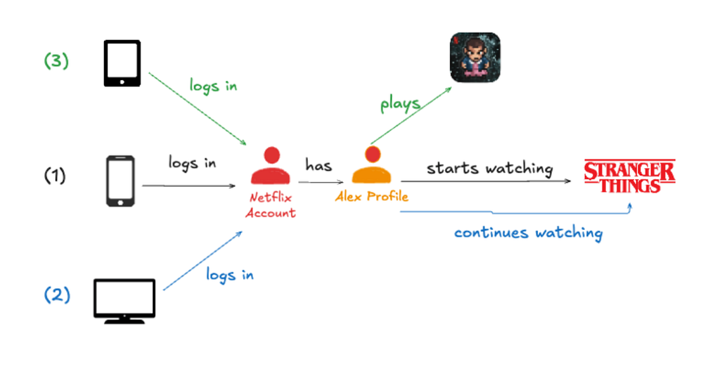
A member journey often looks like this:
In the RDG, this journey creates the following graph structure:
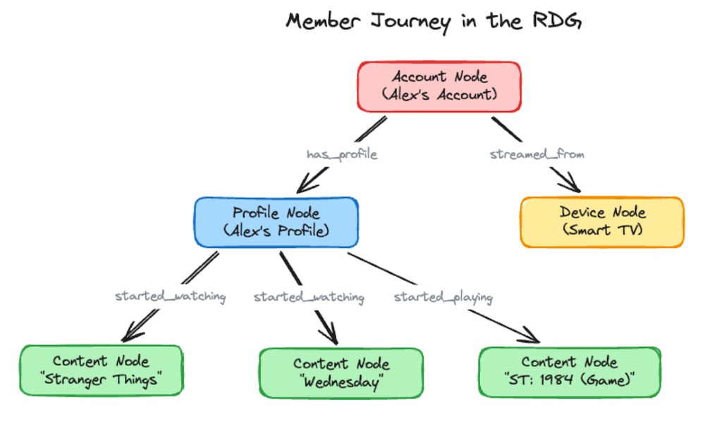
Graph queries vary along two axes: how wide they fan out at each hop, and how deep they chain across hops. To see this range, let’s look at two scenarios from opposite ends:
Consider a “shallow, wide” query: “Which devices has this account used to stream in the last 30 days?”
Using the graph structure above, this translates to:
While this is only a “single hop,” it presents a significant scaling challenge. For a highly active account, the fan-out can be massive. The query layer must fetch hundreds of streamed_from edges, apply temporal filters on each edge’s last_watch_timestamp property to capture only those within the last 30 days, and aggregate the results, all while maintaining sub-100ms latency.
Consider a scenario where personalization teams need to understand a member’s viewing journey. They might ask: “For Account X, show me the Stranger Things viewing history across all profiles: which profiles watched it, what they watched, and when”.
This path unfolds as follows:
The core challenge in this scenario is sequential dependency: we cannot fetch a profile’s viewing history until Hop 1 has identified which profiles exist. In a distributed environment, the client has to wait for Hop 1 to finish before sending Hop 2. If each hop takes 10ms of network time, that’s 20ms of overhead before we’ve processed a single byte. To hit our sub-100ms goal, we needed a way to package this multi-step logic into a single request.
This example is a 2-hop traversal, but queries can chain 3–4 hops across different entity types, and the latency penalty of sequential execution only grows with depth.
These two scenarios pull the system in opposite directions. Shallow-wide queries stress I/O throughput: can we handle massive fan-out without slowing down? Deep-narrow queries stress execution efficiency: can we chain multiple hops without the network overhead adding up? Supporting both on the same system is what shaped the design that follows.
The two scenarios above sit at opposite ends of the spectrum, but they are not unusual. In practice, the RDG serves tens of thousands of queries per second, each potentially different, all needing sub-100ms responses while the underlying graph continues to grow. Scale, latency, query diversity, and the need for extensibility pulled the design in different directions at once, and every choice came with a trade-off we had to live with.
Why breadth-first, not depth-first? The most intuitive way to traverse a graph is depth-first: pick a path, follow it to the end, backtrack, try another path. But in a distributed system where every hop is a network call, depth-first can lead to high latency. If Account X has 5 profiles and each profile has watched hundreds of titles, depth-first would trace all of one profile’s watched titles before moving to the next, missing the opportunity to batch lookups across profiles. Breadth-first flips this by working one level at a time across all nodes, rather than one path at a time through each node. We fetch all profiles for the account at once, then fetch the started_watching edges for all profiles, and finally fetch content details for all matching titles. Three rounds of parallel calls instead of sequential chains. With breadth-first, there is a clear trade-off in memory, because we hold each level of the graph in memory at once, so the cost scales with how wide a level fans out rather than how deep the query goes. We keep this comfortable by bounding each hop with the per-edge-type limits described in Step 5 below, so even a high fan-out level stays a manageable frontier. We’ll walk through how this works, level by level, in Step 3 below.
Why async-first, not thread-per-request? Latency in the RDG is dominated by I/O, reading from the storage layer, calling enrichment services, and waiting on caches. A traditional thread-per-request model would pin a thread to each in-flight query, and most of the time, the thread would be idle, waiting for a network response. With thousands of concurrent queries, we’d need thousands of threads, most of which would be doing nothing. Instead, we decided to build the entire execution pipeline around asynchronous composition. A small set of dedicated thread pools (16–24 threads total) handles thousands of concurrent requests because no thread ever blocks on I/O. While a storage call is in flight, the thread continues with other work and picks up the result when it arrives. This is the foundational design decision on which everything else rests. We’ll see this in action in Step 4 below, where we cover parallel execution.
Why cache selectively, not everything? Not all data in the graph changes at the same rate. Some properties, such as account plan type and content metadata, are relatively stable: they change on the order of hours or days. Edges like who watched what and when change constantly. For stable data that many queries touch, we use a distributed cache (EVCache) with TTLs tuned to data volatility. Getting the caching strategy right took iteration. We started by caching aggressively and measured the impact: tracking hit rates, monitoring stale-data incidents, and adjusting TTLs based on how quickly different node types actually changed in production. The result: 70–80% hit rates on node lookups, achieved by narrowing the cache to nodes that are both frequently accessed and slow to change, while skipping data that would expire before the TTL ran out. Step 6 below covers how this works in practice.
Why opt-in enrichments, not automatic? Clients know what they need. A query checking account relationships doesn’t care about title artwork; a personalization service building a viewing timeline does. Rather than fetching metadata from external services by default and penalizing every query, we make enrichments opt-in: clients specify exactly which external data they want per request. Also, enrichment is fail-open: if a service is slow or unavailable, we return the graph data without it.
Why eventual consistency, not strong? Most of our queries ask “What has this member done recently?”, not “What happened in the last millisecond?” By defaulting to eventual consistency, we read from the nearest replica and avoid coordination overhead. While the RDG is used to power in-the-moment experiences, it is not set up as the source of truth for the data it holds.
The above choices lead to the following three-layer architecture:
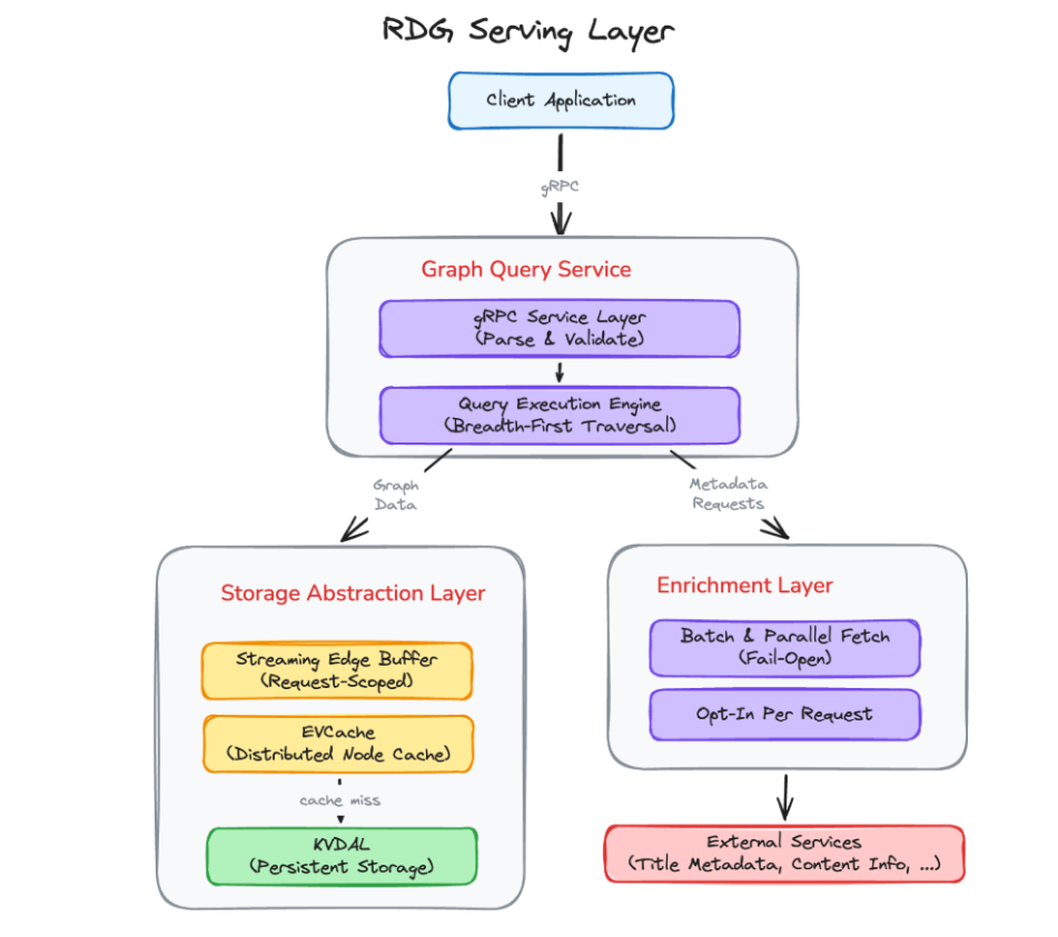
The Graph Query Service is the entry point. It accepts gRPC requests, validates the traversal specification, and hands it to the query execution engine. The execution engine orchestrates breadth-first traversal: expanding one level at a time, applying filters and limits at each hop, and composing all I/O asynchronously.
The Storage Abstraction Layer sits between the execution engine and the underlying KVDAL storage. It provides a clean interface for node lookups and edge retrieval, handles streaming for large adjacency lists, and manages node caching (EVCache).
The Enrichment Layer fetches additional metadata from external Netflix services on demand. It batches requests, runs them in parallel with graph data assembly, and degrades gracefully when an enrichment source is unavailable.
When a client sends a query, the request flows through these layers in sequence: the Query Service parses the request into an execution plan, the execution engine walks the graph level by level through the Storage Abstraction Layer, and if enrichments are requested, the Enrichment Layer fetches and merges external data before the response is serialized back to the client.
Now, with that mental model in place, let’s follow a query through this system and see how these choices play out in practice.
To see how the RDG query layer works in practice, let’s follow a single query end-to-end and focus on one question: how do we make every step fast?
We’ll reuse the deep-narrow example from above:
For Account X, show me the Stranger Things viewing history across all profiles: which profiles watched it, what they watched, and when.
In graph terms, this becomes a 2‑hop traversal:
We’ll walk through how this query moves through the layers we described above:
By the end, we’ll see how a 2-hop query like our Stranger Things example, with streaming, filtering, and parallel execution, can complete in under 100ms.
Every query starts as a gRPC request. Before we touch storage or walk a single edge, the engine needs to understand what the caller actually wants.
For our running example below:
For Account X, show me the Stranger Things viewing history across all profiles
The engine creates a traversal plan with a set of levers: how many hops, how many edges per hop, how much history to consider, and whether to favor recent activity.
We resolve these upfront by merging a hierarchy of filters and limits, from application-level defaults down to per-edge-type overrides, into a concrete execution plan. By the time we read from storage, every hop has clear rules. We’ll see how this hierarchy works in detail in Step 5, but the key insight is simple: interpreting the request up front prevents over-fetching from the downstream storage layer.
Once we’ve parsed the request and decided what the query should do, the next step is to actually touch the graph. For our running example:
For Account X, show me the Stranger Things viewing history across all profiles…
The first concrete question the engine has to answer is very simple:
Which profiles does Account X have?
Under the covers, that really means: how do we find all relevant edges for Account X without scanning the entire graph every time?
If we stored every edge in one massive table, the naive approach would be to scan for rows where source = Account X. Even with indexing, doing that across billions of edges for every request would be slow.
Instead, we organize edges as adjacency lists. For each node, we keep a compact list of “who it’s connected to” by edge type. For Account X, a simplified view might look like:
Account_X: has_profile → [Profile_Alex, Profile_Kids, …,]
Now “get all profiles for Account X” is no longer a global search; it’s a direct lookup into Account X’s stored adjacency. The storage layer can usually pull that list back in a few milliseconds because it’s reading a small, well‑indexed slice of data instead of hunting through everything.
For our query, the first hop is quick: Account X has just two profiles. The engine fetches those edges with has_profile and moves on. For more information on Storage, refer to our previous post.
The first hop was small, but the second is where things get interesting. Each profile can have a large number of started_watchingedges. Loading the entire adjacency list at once would spike latency and memory usage.
To avoid this, we treat adjacency lists as streams rather than blobs.
When the engine requests Profile_Alex’s started_watching edges, the storage layer streams them in batches of 100. As each batch arrives, we apply filters (e.g., “last 30 days”) and decide whether to continue.
If we’ve collected enough edges to satisfy the query’s limits ( max_edge_cnt, lookback window, etc.), we stop reading. Otherwise, we pull the next batch.
In our Stranger Things example:
These two choices, the adjacency‑list lookups and streaming fan‑out, enable everything that follows:
By Step 3, we’re working with concise frontiers like “Profile_Alex and Profile_Kids,” ready for the next hop into their viewing histories.
We’ve completed the first hop. From Account X, we pulled the has_profile edges and found two profiles: Profile_Alex and Profile_Kids.
But we’re not done. The query was:
For Account X, show me the Stranger Things viewing history across all profiles: which profiles watched it, what they watched, and when
So we still need to fetch each profile’s history and filter it down to Stranger Things sessions. As we covered in our design choices, we use breadth-first traversal: expanding all nodes at the current level in parallel before moving to the next.
Let’s walk through the Stranger Things query level by level.
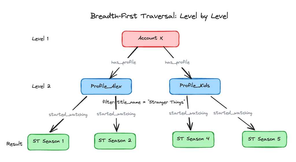
Level 1: Account → Profiles
Starting at Account X, the engine pulls has_profile edges, discovering two profiles:
These become the frontier for Level 2, a single small lookup that takes a few milliseconds.
Level 2: Profiles → Content (Stranger Things)
From those two profiles, we fetch started_watchingedges and filter for Stranger Things. Instead of exhausting Profile_Alex’s entire viewing history before touching Profile_Kids, we treat this as one logical step:
We discover that Profile_Alex watched Season 1 and Season 2, while Profile_Kids watched Season 4. Level 2 turns “2 profiles” into “a handful of Stranger Things sessions” in roughly one storage round trip.
The traversal completes: two levels, two frontiers.
We parallelize within each phase, then regroup. This provides:
For a 2-hop query: two rounds of parallel lookups instead of hundreds of sequential ones. That’s why our Stranger Things query completes in under 100ms.
Breadth-first traversal enables parallel work at each level, which is the key to low latency.
At Level 2 of our Stranger Things query, we fetch started_watching edges for each profile. With two profiles, this is trivial, but in production queries fan out across many profiles, each with hundreds of edges to stream and filter. So do we process them sequentially or in parallel? Sequential means waiting for each profile before starting the next, and the delays stack up. Parallel finishes in the time of the single slowest profile, but hundreds of queries doing this at once could overwhelm storage with unbounded concurrency.
The goal: parallel speed without unbounded chaos.
We structured the query engine like a professional kitchen, with specialized stations for appetizers, mains, and desserts, each with its own capacity. If one station is slammed, the others keep flowing. In practice, that means dedicated thread pools for different work types: fetching nodes, reading adjacency lists, and performing enrichments. When the Stranger Things query reaches Level 2, calls route to the adjacency-list pool, where 8 workers stream and filter each profile’s edges in parallel.
Thread pools give us local control, but we also need a global view of total capacity, so we use adaptive concurrency limiting. When things are healthy, we raise the limit gradually (100 in-flight, then 101, 102, and so on); when timeouts or errors spike, we back off by a larger step (say, 100 down to 70). Combined with per-pool limits, the engine constantly tunes parallelism, fanning out within each level while staying inside safe storage and network limits.
If the client opted into enrichments (say, maturity ratings for the matched content), the Enrichment Layer fetches them in parallel on its own thread pool and merges them into the response. Enrichment is fail-open: a slow or unavailable source never blocks the query, and we just return the graph data without it.
We’ve traversed from Account X to profiles, then to their viewing histories. But raw edges aren’t what our partners need. They care about recent, relevant activity, not every started_watching edge accumulated over the years. This is where filtering decides which parts of the story make the final cut.
Go back to the original question:
For Account X, show me the Stranger Things viewing history across all profiles: which profiles watched it, what they watched, and when.
The phrase “viewing history” is deceptively simple. Under the hood, it means we need to:
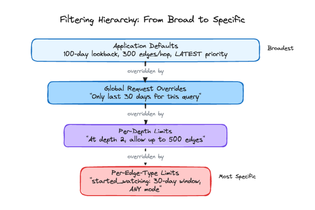
We handle this with a filtering hierarchy. The system starts with conservative defaults (e.g., 100-day lookback, 300 edges per hop), and requests can override them globally, per-hop, or down to specific edge types. In our query, the 100-day default applies broadly, but the caller sets 30 days for started_watching edges, and the narrower rule wins. Older sessions are discarded. The same engine can just as easily provide a tight recent window on one edge type and full history on another, all in a single query.
Sometimes there are still more edges than we want to return after time filtering. If Profile_Alex watched the same episode several times last month, pausing and resuming, we don’t want to send all those edges back. So we offer two selection modes.
LATEST sorts edges by timestamp and keeps the newest ones up to the limit, ideal for “what has this profile watched recently?” where teams want the current state, not every play event. ANY grabs whichever edges it encounters first, no sorting, which is faster and fine for “has this profile ever watched Stranger Things?” where timing doesn’t matter. Teams default to LATEST and switch specific edge types to ANY when “any proof” is enough.
So what happens for our running query?
We start with all the started_watching edges for each profile. The time filter narrows this to 30 days. Edge-count limits prevent response flooding. LATEST mode selects the most recent viewing session per title. The result: a concise answer distilled from a verbose history:
This filtering turns raw history into a focused answer.
By now, we’ve walked the full path of our query: we’ve traversed from account to profiles, filtered viewing history by time, and focused on Stranger Things sessions.
Despite our optimizations, each storage call still costs a network round-trip. When the same nodes appear across thousands of queries per minute, those redundant calls add up: both in infrastructure cost and in tail latency at scale.
The key question: what can we avoid repeating?
Look back at the entities in our Stranger Things journey:
These rarely change. Profiles don’t flip between “kids” and “non-kids” every minute. Title metadata is stable.
To improve efficiency, we keep a distributed cache of hot nodes (accounts, profiles, content) that are likely to reappear. When the same entity appears again, we answer “What is this node?” from memory, skipping storage.
Result: for high-traffic entities, we eliminate storage calls and noticeably reduce infrastructure cost and tail latency at scale.
The first time the Stranger Things query runs for Account X, the cache is cold, so we pay the full cost: we fetch the account and its profiles, then the started_watching edges and matching content nodes, caching each node as we go. Minutes later, a different query arrives:
Show me everything Account X’s profiles have watched in the last 7 days, and flag anything rated TV-MA on the kids profile.
This time, many of those nodes are already in the distributed cache. Storage still handles the adjacency lists and edges, but node lookups are lighter and latency drops. At scale, that reuse gives us comfortable headroom for traffic spikes.
We can’t cache everything. The RDG prunes old activity after a set retention window, so caching a node that’s about to be deleted is wasteful.
To avoid polluting the cache, we consider:
If a node was last active 99 days ago, it expires from the graph in a day, so a 30-day TTL makes no sense, and we skip it. We reserve cache space for active nodes like Account X. This “smart TTL” policy keeps the cache focused on live stories rather than archival ones, so repeat queries for the same part of the graph return faster.
Caching is integrated into the journey, not an afterthought. The engine reuses knowledge from previous queries, so repeated traversals over the same part of the graph keep getting cheaper
The serving layer sits in front of 8 billion nodes and 150 billion edges, serving mixed workloads, all of which need to feel interactive. Single-hop queries return at a P50 of 15–30ms with P99 under 100ms. Even 3-hop traversals, the kind that chain across accounts, profiles, and content, come back at P99 between 100–150ms. Breadth-first execution and parallelism within each level keep these numbers stable even as fan-out grows.
The async-first design is what enables the throughput. Thousands of concurrent requests flow through just 16–24 threads spread across dedicated pools because no thread ever blocks on I/O. When load spikes, our concurrency limiter lets work queue briefly: slowly increasing capacity when things are healthy, backing off aggressively when they’re not
Caching has the most visible impact on day-to-day efficiency. Popular entities like accounts, profiles, and content achieve 70–80% cache hit rates, resulting in roughly 3–4x fewer storage calls on common query paths. Smart TTLs keep the cache focused on active data, avoiding wasted memory on nodes that are near the end of their graph retention window.
These properties, together, make multi-hop graph queries over billions of entities feel, at query time, much closer to in-memory lookups than to remote calls.
The biggest surprise wasn’t any single optimization: it was how much async composition changed the economics of our system. We expected it to help latency; we didn’t expect it to slash infrastructure cost. A serving layer that would have needed hundreds of threads per instance runs comfortably on 16–24, because no thread ever blocks on I/O. The tradeoff is debuggability: async stack traces are hard to read, and exceptions can get lost in future chains. We compensated with per-stage metrics, measuring each request at validation, storage, enrichment, and end-to-end, so when something is slow, we know exactly which stage to blame.
Caching took longer to get right than expected. Our first instinct was to cache everything in EVCache and let TTLs handle freshness, but that wastes memory on nodes about to expire from the graph anyway. The breakthrough was matching TTLs to data volatility: stable node properties get long TTLs, while nodes near the end of their retention window aren’t cached at all. The 70–80% hit rate we see today came from being selective, not aggressive.
The filtering hierarchy was born out of frustration. Early on, every new use case meant a code change: one team wanted a 7-day lookback, another 90 days, a third different limits at different depths. Instead of bespoke logic per team, we built a layered override system: application defaults, global overrides, per-depth limits, and per-edge-type limits. It took real effort, but it eliminated an entire class of feature requests and teams now tune their own queries without touching our code.
The lessons above are specific to the RDG, but the underlying principles apply to any distributed system built around I/O-heavy, fan-out workloads.
—
Thanks for reading Part 3 of the RDG blog series. For us, getting these details right is what turns a constantly changing, billion-edge graph into something that, at query time, feels like a responsive, in-memory data structure.

How and Why Netflix Built a Real-Time Distributed Graph: Part 3 — Querying the graph with gRPC… was originally published in Netflix TechBlog on Medium, where people are continuing the conversation by highlighting and responding to this story.
Post Syndicated from LastWeekTonight original https://www.youtube.com/watch?v=vo7cYJHVpUQ
Post Syndicated from jzb original https://lwn.net/Articles/1086949/
The shadow-utils
project provides the tools that handle /etc/shadow,
/etc/passwd, and other related databases; in
general, manages users and groups on many Linux systems. While most
software releases are notable for what is added, the recent shadow-utils 4.20.0
release is most noteworthy for what has been removed. Specifically,
several utilities and functionality related to periodic password
expiry, which were deprecated in the December 2025 4.19.0
release, have been removed as planned. It is still possible to manage
some aspects of password aging with shadow-utils, but organizations
that depend on such features should start planning for their complete
removal within a few years.