Post Syndicated from Markku Leiniö original https://blog.zabbix.com/zabbix-7-0-proxy-load-balancing/28173/

One of the new features in Zabbix 7.0 LTS is proxy load balancing. As the documentation says:

Proxy load balancing allows monitoring hosts by a proxy group with automated distribution of hosts between proxies and high proxy availability.

If one proxy from the proxy group goes offline, its hosts will be immediately distributed among other proxies having the least assigned hosts in the group.

Proxy group is the new construct that enables Zabbix server to make dynamic decisions about the monitoring responsibilities within the group(s) of proxies. As you can see in the documentation, the proxy group has only a minimal set of configurable settings.

One important background information to understand is that Zabbix server always knows (within reasonable timeframe) which proxies in the proxy groups are online and which are not. That’s because all active proxies connect to the Zabbix server every 1 second by default (DataSenderFrequency setting in the proxy), and Zabbix server connects to the passive proxies also every 1 second by default (ProxyDataFrequency setting in the server), so if those connections are not happening anymore, then something is wrong with using the proxy.

Initially Zabbix server will balance the hosts between the proxies in the proxy group. It can also rebalance the hosts later if needed, the algorithm is described in the documentation. That’s something we don’t need to configure (that’s the “automated distribution of hosts” mentioned above). The idea is that, at any given time, any host configured to be monitored by the proxy group is monitored by one proxy only.

Now let’s see how the actual connections work with active and passive Zabbix agents. The active/passive modes of the proxies (with the Zabbix server connectivity) don’t matter in this context, but I’m using active proxies in my tests for simplicity.

Disclaimer: These are my own observations from my own Zabbix setup using 7.0.0, and they are not necessarily based on any official Zabbix documentation. I’m open for any comments or corrections in any case.

At the very end of this post I have included samples of captured agent traffic for each of the cases mentioned below.

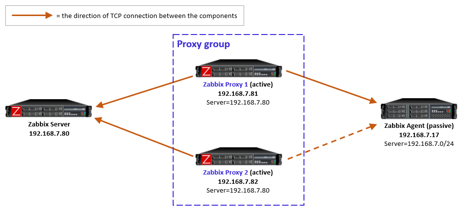
Passive agents monitored by a proxy group

For passive agents the proxy load balancing really is this simple: Whenever a proxy goes down in a proxy group, all the hosts that were previously monitored by that proxy will then be monitored by the other available proxies in the same proxy group.

There is nothing new to configure in the passive agents, only the usual Server directive to allow specific proxies (IP addresses, DNS names, subnets) to communicate with the agent.

As a reminder, a passive agent means that it listens to incoming requests from Zabbix proxies (or the Zabbix server), and then collects and returns the requested data. All relevant firewalls also need to be configured to allow the connections from the Zabbix proxies to the agent TCP port 10050.

As yet another reminder, each agent (or monitored host) can have both passive and active items configured, which means that it will both listen to incoming Zabbix requests but also actively request any active tasks from Zabbix proxies or servers. But again, this is long-existing functionality, nothing new in Zabbix 7.0.

Active agents monitored by a proxy group

For active agents the proxy load balancing needs a bit new tweaking in the agent side.

By definition, an active agent is the party that initiates the connection to the Zabbix proxy (or server), to TCP port 10051 by default. The configuration happens with the ServerActive directive in the agent configuration. According to the official documentation, providing multiple comma-separated addresses in the ServerActive directive has been possible for ages, but it is for the purpose of providing data to multiple independent Zabbix installations at the same time. (Think about a Zabbix agent on a monitored host, being monitored by both a service provider and the inhouse IT department.)

Using semicolon-separated server addresses in ServerActive directive has been possible since Zabbix 6.0 when Zabbix servers are configured in high-availability cluster. That requires specific Zabbix server database implementation so that all the cluster nodes use the same database, and some other shared configurations.

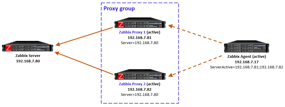
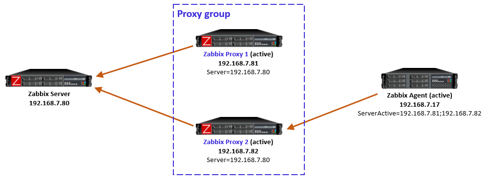
Now in Zabbix 7.0 this same configuration style can be used for the agent to connect to all proxies in the proxy group, by entering all the proxy addresses in the ServerActive configuration, semicolon-separated. However, to be exact, this is not described in the ServerActive documentation as of this writing. Rather, it specifically says “More than one Zabbix proxy should not be specified from each Zabbix server/cluster.” But it works, let’s see how.

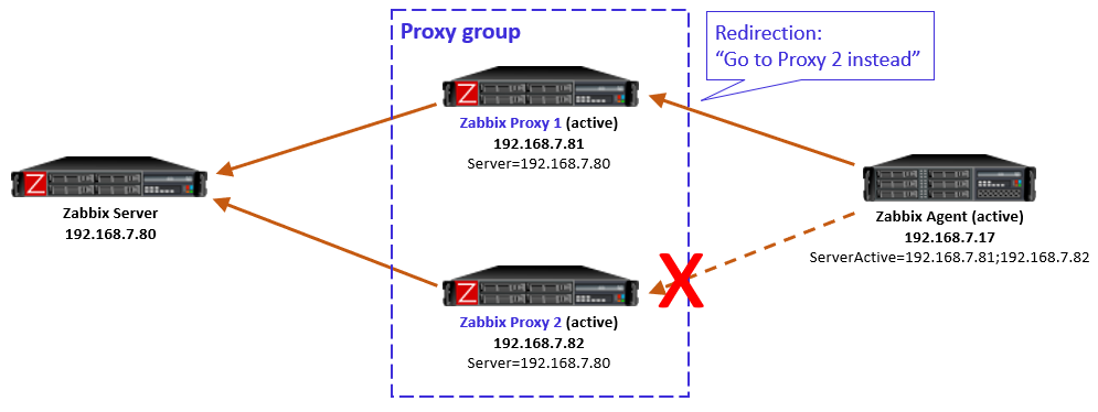
Using multiple semicolon-separated proxy addresses works because of the new redirection functionality in the proxy-agent communication: Whenever an active agent sends a message to a proxy, the proxy tells the agent to connect to another proxy, if the agent is currently assigned to some other proxy. The agent then ceases connecting to that previous proxy, and starts using the proxy address provided in the redirection instead. Thus the agent converges to using only that one designated proxy address.

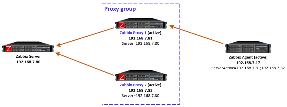
In this simple example the Zabbix server determined that the agent should be monitored by Proxy 1, so when the agent initially contacted Proxy 1 (because its IP address is first in the ServerActive list), the proxy responded normally and agent was happy with that.

In case the Zabbix server had for any reason determined that the agent should be monitored by Proxy 2, then Proxy 1 would have responded with a redirection, and agent would have followed that. (There will be examples of redirections in the capture files below.)

To be clear, this agent redirection from the proxy group works only with Zabbix 7.0 agents as of this writing.

Note: In the initial version of this post I used comma-separated proxy addresses in ServerActive (instead of semicolon-separated), and that caused duplicate connections from the agent to the designated proxy (because the agent is not equipped to recognize that it connects to the same proxy twice), eventually causing data duplication in Zabbix database. Using comma-separated proxy addresses is thus not a working solution for proxy load balancing usage.

If the host-proxy assignments are changed by the Zabbix server for balancing the load between the proxies, the previously designated proxy will redirect the agent to the correct proxy address, and the situation is optimized again.

Side note: When configuring the proxies in Zabbix UI, there is a new Address for active agents field. That is the address value that is used by the proxies when responding with redirection messages to agents.

Proxy group failure scenarios with active agents

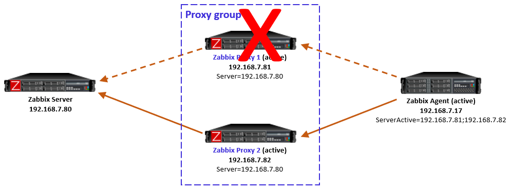
Proxy goes down

If the designated proxy of an active agent goes offline so that it doesn’t respond to the agent anymore, agent realizes the situation, discards the redirection information it had, and reverts to using the proxy addresses from ServerActive directive again.

Now, this is an interesting case because of some timing dependencies. In the proxy group configuration there is the Failover period configuration that controls the Zabbix server’s sensitivity to proxy availability in regards to agent rebalancing within the proxy group. Thus, if the agent reverts to using the other proxies faster than Zabbix server recognizes the situation and notifies the other proxies in the proxy group, the agent will get redirection responses from the other proxies, telling it to use the currently offline proxy. And the same happens again: agent fails to connect to the redirected proxy, and reverts to using the other locally configured proxies, and so on.

In my tests this looping was not very intense, only two rounds every second, so it was not very significant network-wise, and the situation will converge automatically when the Zabbix server has notified the proxies about the host rebalancing.

So this temporary looping is not a big deal. The takeaway is that the whole system converges automatically from a failed proxy.

After the failed proxy has recovered to online mode, the agents stay with their designated proxies in the proxy group.

As mentioned in the beginning, Zabbix server will automatically rebalance the hosts again after some time if needed.

Proxy is online but unreachable from the active agent

Another interesting case is one where the proxy itself is running and communicating with Zabbix server, thus being in online mode in the proxy group, but the active agent is not able to reach it, while still being able to connect to the other proxies in the group. This can happen due to various Internet-related routing issues for example, if the proxies are geographically distributed and far away from the agent.

Let’s start with the situation where the agent is currently monitored by Proxy 2 (as per the last picture above). When the failure starts and agent realizes that the connections to Proxy 2 are not succeeding anymore, the agent reverts to using the configured proxies in ServerActive, connecting to Proxy 1.

But, Proxy 1 knows (by the information given by Zabbix server) that Proxy 2 is still online and that the agent should be monitored by Proxy 2, so Proxy 1 responds to the agent with a redirection.

Obviously that won’t work for the agent as it doesn’t have connectivity to Proxy 2 anymore.

This is a non-recoverable situation (at least with the current Zabbix 7.0.0) while the reachability issue persists: The agent keeps on contacting Proxy 1, keeps receiving the redirection, and the same repeats over and over again.

Note that it does not matter if the agent is now locally reconfigured to only use Proxy 1 in this situation, because the load balancing of the hosts in the proxy group is not controlled by any of the agent-local configuration. The proxy group (led by Zabbix server) has the only authority to assign the hosts to the proxies.

One way to escape from this situation is to stop the unreachable Proxy 2. That way the Zabbix server will eventually notice that Proxy 2 is offline, and the hosts will be automatically rebalanced to other proxies in the group, thus removing the agent-side redirection to the unreachable proxy.

Keep this potential scenario in mind when planning proxy groups with proxy location diversity.

This is also something to think about if your Zabbix proxies have multiple network interfaces, where Zabbix server connectivity is using different interface from the agent connectivity. In that case the same problem can occur due to your own configurations.

Closing words

All in all, proxy load balancing looks very promising feature as it does not require any network-level tricks to achieve load balancing and high availability. In Zabbix 7.0 this is a new feature, so we can expect some further development for the details and behavior in the upcoming releases.

---

Appendix: Sample capture files

Ideally these capture files should be viewed with Wireshark version 4.3.0rc1 or newer because only the latest Wireshark builds include support for latest Zabbix protocol features. Wireshark 4.2.x should also show most of the Zabbix packet fields. Use display filter “zabbix” to see only the Zabbix protocol packets, but when examining cases more carefully you should also check the plain TCP packets (without any display filter) to get more understanding about the cases.

These samples are taken with Zabbix components version 7.0.0, using default timers in the Zabbix process configurations, and 20 seconds as the proxy group failover period.

Passive agent, with proxy failover

• • After frame #50 Proxy 1 was stopped and Proxy 2 eventually took over the monitoring

Active agent, with proxy failover

• • The agent initially communicates with Proxy 1
  • Proxy 1 was stopped before frame #425
  • Agent connected to Proxy 2, but Proxy 2 keeps sending redirects
  • Proxy 2 was assigned the agent before frame #1074, so it took over the monitoring and accepted the agent connections
  • Proxy 1 was later restarted (but agent didn’t try to connect to it yet)
  • The agent was manually restarted before frame #1498 and it connected to Proxy 1 again, was given a redirection to Proxy 2, and continued with Proxy 2 again

Active agent, with proxy unreachable

• • Started with Proxy 2 monitoring the agent normally
  • Network started dropping all packets from the agent to Proxy 2 before frame #179, agent started connecting to Proxy 1 almost immediately
  • From frame #181 on Proxy 1 responds with redirection to Proxy 2 (which is not working)
  • Proxy 2 was eventually stopped manually
  • Redirections continue until frame #781 when Proxy 1 is assigned the monitoring of the agent, and Proxy 1 starts accepting the agent requests

This post was originally published on the author’s blog.

The post Zabbix 7.0 Proxy Load Balancing appeared first on Zabbix Blog.