Tag Archives: Kubernetes

Migrating Counter Service storage: Design choices and learnings

Post Syndicated from Grab Tech original https://engineering.grab.com/counter-service-storage-migration

Introduction

Counter Service is used across Grab’s anti-fraud platform to answer time-windowed count questions, such as recent ride requests by a user or failed payment attempts on a card. The service handles tens of thousands of queries per second (QPS) with about a billion requests per day, while maintaining strict requirements around latency and reliability to support real-time fraud rule evaluation.

For most of its life, Counter Service was backed by a wide-column database that served the workload reliably as the service scaled. As part of a broader infrastructure review mandated at an organizational level, our database team evaluated alternatives to this storage that many services relied on, including Counter Service. Based on their assessment, Aerospike emerged as a good fit for our use-case. We also used the migration as an opportunity to decouple storage concerns from business logic, a necessary first step for this migration, and one that would reduce the effort required for future storage changes. As part of the same effort, we revisited the data model and access patterns in detail, which helped us identify and apply several straightforward optimizations.

This post walks through how we did it. What we built on the reader-side to make the migration safe, how we redesigned the writer-side data model around the new backend, and what we ran into during the gradual rollout.

Setting the stage

Counter data is stored in three time granularities: 15-minute, hourly, and daily buckets. A typical read would be along the lines of, “give me the count for key X over the last 90 minutes”, which the service decomposes into the smallest possible set of buckets, one hourly in the middle, a few 15-minute buckets at the edges, fetches them, and sums.

In the original setup, each granularity was stored in a separate table with a composite primary key:

TABLE daily_count (
    key      TEXT,         -- partition key
    day_ts   TIMESTAMP,    -- clustering key
    count    BIGINT,
    PRIMARY KEY (key, day_ts)
);

The clustering column gave us convenient range queries, that is needed for the Counter Service. On the write path, each incoming counter event triggered a read-modify-write, three parallel SELECT across the three tables, an in-memory increment, then a batch write. This produced four network round-trips per event.

As this service is a core part of Grab’s fraud detection ecosystem and handles high query volume, migrating its underlying storage required a careful rollout plan. We had three requirements:

  • Ramp traffic to the new backend gradually and roll back at any point with a config change.
  • Monitor both the original and new storage paths to verify data integrity before switching over.
  • Complete the migration without downtime.

We also wanted the migration machinery to be reusable for future storage changes. The migration is divided into three workstreams, which we’ll walk through below:

  • Preparing the reader service.
  • Identifying the best integration mechanism for the new storage.
  • Updating the writer pipeline.

Reader: Separating the data access layer

The reader is a Rust service. Before any migration work began, the reader’s business logic had tight coupling with the storage layer. Session creation, query building, fan-out orchestration, and the data types those queries returned were all intertwined in a single flat file. The main application state struct (AppState) held a raw database session handle and prepared query references. Every handler, gRPC Remote Procedure Calls (gRPC) or HyperText Transfer Protocol (HTTP), received the bare session as a parameter. Variable names baked the storage technology into the business layer.

This made the storage migration difficult to attempt directly. We couldn’t add a second storage backend without forking the orchestration logic, and we had no way to test the read path in isolation from a real database session. So we did the migration prep in three stages.

Stage 1: Extracting the storage code

The first stage shipped no behavioural change. We deleted the monolithic storage file and split its contents in two:

  • storage/legacy.rs: wrapped session creation, prepared statements, and query execution behind a LegacyStorage struct.
  • batch_read_ops.rs: kept only the orchestration logic: time-range splitting, channel-based fan-out, and aggregation.

AppState started holding an Arc<LegacyStorage> instead of a raw session handle. The PreparedQueries struct lost its statements (those moved inside LegacyStorage). We renamed every storage-specific identifier in business code to generic storage_* names.

The result was a hard fence. After Stage 1, the database driver crate was reachable only from inside the storage module. Nothing in the business logic or handlers imported it any more.

Stage 2: The storage facade

With the seam in place, we introduced the actual abstraction. A new storage/ module with mod.rs, legacy.rs, aerospike.rs, and mock_storage.rs as siblings became the only place driver crates were reachable from.

The idiomatic Rust approach would have been a trait with associated types, but our backend selection is runtime (a config string parsed at startup), and associated types propagate upwards through every consumer. The alternative, trait objects with boxed futures adds a heap allocation per query, which we wanted to avoid at our QPS.

We chose a concrete facade with enum dispatch:

struct Storage {
    legacy:    LegacyStorage,
    aerospike: AerospikeStorage,
    mock:      MockStorage,
    settings:  StorageSettings,
}

execute_queries(backend: BackendType, ...) {
    match backend {
        Legacy    => self.legacy.execute(...),
        Aerospike => self.aerospike.execute(...),
        Mock      => self.mock.execute(...),
    }
}

A match statement at the request boundary, which made it easier to reason about and debug. The facade then routes everything to the original backend without the rest of the code knowing or caring.

Each backend’s execute_queries honours the same contract: take a Vec<QueryCandidate> and a HashMap<BatchIndex, Sender<...>>, and emit (index, value, timestamp, granularity) tuples into those channels. The orchestration layer above doesn’t need to know whether a candidate became a paginated row stream or a single batch read with client-side map filtering, both write into the same channels in the same shape.

On top of the facade we layered three config-driven operating modes that map to the migration phases:

  • Single: one backend serves the request.
  • WithShadow: the primary serves the response; the secondary runs asynchronously in the background for parity comparison.
  • WithSplit: a deterministic percentage of traffic is served by each backend. Used for the live cutover.

The mode and traffic percentages are read from a service config, allowing the reader to move from legacy-only to Aerospike-only without code changes. The transition starts in Single(legacy), then shadow reads are enabled with WithShadow(primary=legacy, secondary=aerospike, pct=X). The shadow percentage is gradually ramped from 5% to 20%, 50%, and finally 100%, while parity is verified through metrics. Optionally, the system can then move into WithSplit(primary=legacy, secondary=aerospike, split=X), where live traffic is gradually shifted from the original backend to Aerospike, for example from 5% to 30%, 70%, and then 100%. Once Aerospike is fully validated and serving all traffic, the reader moves to Single(aerospike).

Stage 3: Shadow comparison and metrics

Each storage call carries metadata like backend, role (primary/secondary/shadow), and mode, attached as tags to every metric. When Aerospike was added, existing dashboards showed per-backend breakdowns without changes.

We placed the mode dispatch at the handler level rather than inside the storage layer to validate the full request path, not only the rows returned by storage. This also lets the response return as soon as the primary completes, while the shadow runs as a fire-and-forget background task.

Writer: redesigning the data model

Since the two systems use different storage engines, it wasn’t clear that a one-to-one port of our original schema would work. We tried three approaches.

Approaches 1 and 2: Row-per-bucket

We first tried mirroring our original row-per-bucket model. Approach 1 used Aerospike’s Secondary Index (SI) to recover range queries; approach 2 skipped SI and computed the exact set of primary keys client-side via BatchGet.

Both hit the same wall: Aerospike’s primary index is 64 bytes per record, kept in memory. At billions of records, index memory becomes the constraint. SI added overhead and operational complexity we didn’t need.

Approach 3: Map-based schema

The third approach was structurally different from the first two and was the most compact of the options. Rather than storing one record per bucket, which kept us in the same cardinality regime, we collapsed all bucket counts for a single counter into one record. The values were stored as a sorted map keyed by bucket timestamp:

Set:           helium_hourly
Primary key:   "{counterKey}"
Bins:
   counts: KEY_ORDERED_MAP({
        1773369000000: 1,
        1773372600000: 3,
        1773376200000: 7,
        ...
   })

The map keys are bucket timestamps in milliseconds. The map values are running counts. One record holds the entire time series for one counter at one granularity.

Reads become straightforward: fetch the record, iterate the map, sum the entries within the requested window. Each Get returns a bounded number of map entries (determined by Time To Live (TTL) and bucket size), and client-side filtering of that many entries is negligible.

Writes use MapIncrementOp, an atomic server-side increment of a value at a given map key, creating the entry on first access. Combined with MapRemoveByKeyRangeOp for pruning stale entries, every write is one atomic operation:

ops = [
    MapIncrementOp(counts, bucketTsMs, delta),
    MapRemoveByKeyRangeOp(counts, 0, cutoffMs),
    PutOp(key_bin, counterKey),
]
client.Operate(policy, key, ops)

For TTL management, we couldn’t use Aerospike’s record-level expiry directly. A single record holds many timestamps, so record-level TTL would either keep everything or drop everything. Instead, we prune stale map entries explicitly on every write using MapRemoveByKeyRangeOp. The record-level TTL stays as a safety net for counters that stop receiving writes.

The two backends produce very different network shapes for the same logical query. The original backend returns many small paginated row streams, one per (key, granularity). The server filters by time range using the clustering column. Aerospike returns one batch response with the entire counts map per key, and the client filters the map to the requested range. The reader’s storage layer hides this difference: both paths emit (index, value, timestamp, granularity) tuples into the same per-index channels, and the orchestrator above sums them the same way.

The third approach performed best in testing. By collapsing many bucket records into a single record per counter, we reduced the total record count by more than an order of magnitude, which also reduced primary index memory. It also produced a smaller on-disk footprint, since the long counter key is stored once per record instead of being repeated across every bucket. The schema was chosen to fit the access pattern, with the index and disk savings following naturally.

The pipeline continues writing to the original backend as the primary, while Aerospike is added as a separate asynchronous shadow write behind a deterministic rollout logic. This lets us ramp Aerospike gradually and eventually cut over to it fully.

Reader: How each backend actually serves a query

The two storage backends sit behind the same execute_queries contract on the reader service, but what they do internally for a single batch read looks very different.
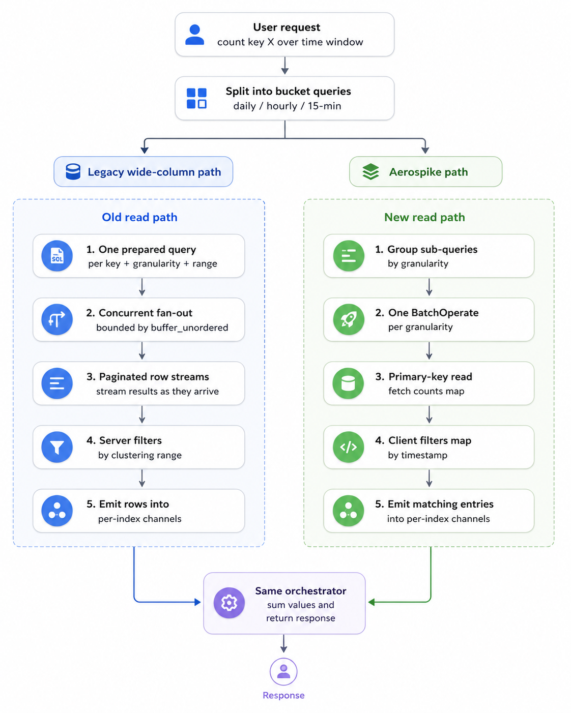
Figure 1. How a single read request flows through each backend.

The reader takes a batch of counter queries and decomposes each into one or more sub-queries per granularity (a 90-minute window for instance, becomes one hourly sub-query and two 15-minute sub-queries). In the original backend, each sub-query becomes its own prepared statement bound with (start_ms, end_ms, key), and the storage layer fires all of them concurrently as a stream of futures with buffer_unordered capping in-flight queries to a tuned bound. Each query returns a paginated row iterator, the server uses the clustering column to filter by time range and rows stream through to per-index channels as they arrive. So a single user request can produce many small queries, each a separate network round-trip to the partition master holding key, with results dribbled back over a paginated stream.

On Aerospike, the storage layer first groups all sub-queries by granularity, then issues one BatchOperate per granularity. Each sub-query becomes a single primary-key read against the appropriate set; the server returns the entire counts map for that key in one record. The client iterates the map and emits only the entries whose timestamps fall inside the requested range. This keeps the code simple, and at our map sizes the overhead is negligible. There’s no streaming, a batch read either succeeds or fails as a unit and there are at most three network round-trips per user request, one per granularity, regardless of how many sub-queries there are.

This reflects the different design philosophies of the two systems. Wide-column stores typically expect client-side fan-out for reads, while Aerospike’s batch API is designed for exactly this multi-key pattern.

A few issues with the Aerospike Rust client also surfaced during rollout, as it was less mature than its Go counterpart. For example, when we started, the officially available Rust client was synchronous, so every batch read had to be bridged through tokio::task::spawn_blocking with some amount of custom plumbing. Once the official async client was released, we removed that layer and saw measurable improvements in both p50 and p99 latency. The other issue was Domain Name System (DNS). The client resolved seed hostnames only during initialization and did not re-resolve them when the cluster topology refreshed. As a result, a full staging cluster replacement, with new IPs behind the same hostnames, left the client stuck on the old IPs until restart. We filed the bug upstream, and a fix shipped in a subsequent release. We also reproduced the scenario locally with a Docker-based end-to-end test and ran additional staging drills to confirm recovery before continuing the rollout.

Experiment with indexing

We run Aerospike in its default storage configuration, Hybrid Memory Architecture (HMA), where the primary index sits in Random-Access Memory (RAM) and the data sits on Solid-State Drive (SSD). The other relevant mode keeps both index and data in Dynamic Random-Access Memory (DRAM), which is more expensive and not something that fits our use-case. Even in HMA, the primary index grows linearly with record count. At our scale, that growth was a foreseeable issue.

To raise the memory ceiling, we tried moving the primary index itself from RAM to local Non-Volatile Memory Express (NVMe) while keeping data on SSD. We expected the extra index latency to be invisible within our overall request budget. In practice, we started seeing p99 spikes that did not track overall QPS. Instead, they followed I/O activity on hot keys. We observed that when many concurrent lookups land on the same record, the in-memory index handles them more prudently compared to a disk backed index. Adding more and better nodes improved things slightly but did not mitigate the issue. Consequently, we reverted back to in-memory index with a memory-optimized instance type.

Overall impact

The migration delivered gains across infrastructure, performance, and data footprint. Most of these improvements trace back to the schema redesign like collapsing rows into maps, rather than the database change itself.

The primary index currently uses about 50 GB of the roughly 100 GB usable memory per node. The same dataset is around 1 TB on disk, compared with around 3 TB on the original setup. This is primarily attributed to our adoption of the map-based schema discussed earlier.

In production, p99 read latency was consistently better than the original setup, with roughly 50% improvement across our read paths. The write path now uses a single atomic increment operation, replacing the read-modify-write pattern we had built previously.

The new setup costs roughly 45–50% less per node compared to our original setup. We also reduced the replication factor from 3 to 2, saving roughly a third of both storage and primary index memory. RF=2 can be awkward in databases that depend on write quorum, but Aerospike’s master-replica model still keeps an authoritative copy available after a single-node loss. That gives us meaningful fault tolerance even at RF=2. The remaining risk, a simultaneous multi-AZ failure, was acceptable for this workload because the writer continues producing increments from the source event stream. Any lost counter data can self-heal as new events arrive.

Conclusion

This migration ultimately came down to aligning the storage design with the workload. These results would not have been achieved by simply swapping one storage system for another. As the service evolved over time, our initial design choices became less optimal, and the migration surfaced opportunities to rethink them. The gains came from focusing on optimization opportunities, redesigning the data model, and cleanly separating storage concerns. Through shadow reads and writes, followed by a gradual rollout, we completed the migration with zero downtime and no data-integrity issues. The result is a system that fits its workload well and a foundation that makes future storage changes safer and easier to attempt.

Join us

Grab is Southeast Asia’s leading superapp, serving over 900 cities across eight countries (Cambodia, Indonesia, Malaysia, Myanmar, the Philippines, Singapore, Thailand, and Vietnam). Through a single platform, millions of users access mobility, delivery, and digital financial services, including ride-hailing, food delivery, payments, lending, and digital banking via GXS Bank and GXBank. Founded in 2012, Grab’s mission is to drive Southeast Asia forward by creating economic empowerment for everyone while delivering sustainable financial performance and positive social impact.

Powered by technology and driven by heart, our mission is to drive Southeast Asia forward by creating economic empowerment for everyone. If this mission speaks to you, join our team today!
How Netflix Simplified Batch Compute with Kueue

Post Syndicated from Netflix Technology Blog original https://netflixtechblog.com/how-netflix-simplified-batch-compute-with-kueue-87860682629c

By Alvin Bao, Alex Petrov, Jennifer Lai, Aidan Sherr, and Samartha Chandrashekar

As a part of the journey to transition Netflix’s compute infrastructure to be more Kubernetes-native, we have leaned into incorporating components from the Kubernetes ecosystem into our container platform Titus. One example of this is our use of Kueue, a cloud-native job queueing system for batch workloads, which has largely replaced the custom queuing and scheduling logic in our homegrown managed batch solution Compute Managed Batch (CMB). In this post, we’ll give an overview of what motivated the migration, how we migrated millions of batch jobs to use Kueue, and what Kueue allows us to offer as a Compute platform.

Brief Overview of CMB and Titus

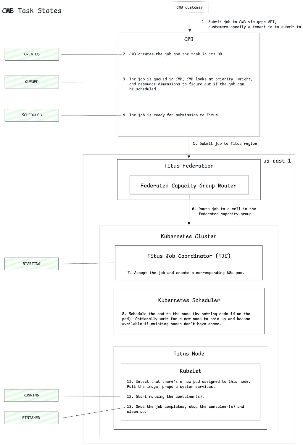
CMB is a managed batch solution that allows users and applications to execute and manage workloads that run to completion. Using a tenant hierarchy, workloads are managed and queued with ordered execution through priorities, and capacity is managed on a per-tenant basis. Workloads that are submitted to CMB are then run on Titus. The features of Titus relevant to CMB are workload federation across multiple cells (Kubernetes clusters) and federated capacity reservations. This means CMB can talk to a single Titus endpoint to get/submit workloads and update capacity reservations without having to worry about the underlying cell/cluster topology.

CMB Tenant Hierarchy

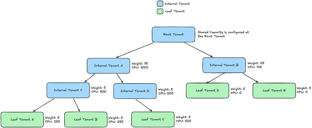
Tenants provide a grouping mechanism for jobs submitted on behalf of certain organizations, platforms, or applications. Users can create and organize tenants however best suits their organization or use case. For example, an organization may use a single tenant across several applications or a complex hierarchical structure that matches its team and application ownership structure.

Tenants are associated with a capacity configuration. The capacity configuration defines the amount of compute capacity available to the tenant and provides certain guarantees around isolation from other tenants. The capacity configuration contains weight (used for fair sharing) and resource dimensions.

There are two types of tenants in CMB:

  1. Internal Tenants — meant to facilitate the creation of a tree of tenants. Internal tenants’ children can be both internal and leaf tenants. Internal tenants themselves do not accept work and thus do not have associated queues.
  2. Leaf Tenants — can accept work and have queues associated with them. Leaf tenants cannot have any children.

With regards to capacity configuration, tenants can use 2 types of capacity:

Reserved Capacity

For internal tenants, if a user specifies reserved capacity, it is fair-shared across the subtree and usable by the leaf tenants under that internal tenant.

For leaf tenants, if a user specifies reserved capacity, it partitions capacity within the hierarchy so that other tenants cannot reserve the same resources. Those reserved resources are not shared with any other tenant, ensuring throughput for a given leaf tenant.

Shared Capacity

The Compute team maintains a global pool of shared capacity that any tenant can burst into, in addition to its reserved capacity. Reservations are not required to use CMB, so a tenant can run out of shared capacity entirely. The pool is fair-shared across tenants, but in CMB, this applied only at admission: CMB had no preemption, so once a job was admitted, it ran to completion regardless of shifts in fair-share demand.

Kueue changes the semantics for both types of capacity, which the fair sharing and preemption section covers.

Here is an example of what a tenant hierarchy looks like:

CMB User/Application Workload Submission Flow

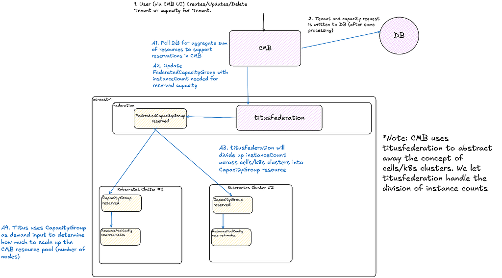
CMB User/Application Tenant Management Flow

Why Kueue?

CMB was created in 2018, before or alongside many of the open-source batch compute offerings available today. Over the years, as the Kubernetes ecosystem has evolved, many of the features that CMB offered or strived to offer have been included in these open source projects e.g., fair sharing, hierarchical tenants, capacity management, priority queuing. In addition, it became increasingly cumbersome to develop new features such as preemption when CMB was so far removed from the underlying Kubernetes cluster.

The team took a look at what it would take to modernize our batch abstraction and settled on Kueue for the following reasons:

  1. Unlike other options such as YuniKorn or Volcano, Kueue does not replace pod scheduling by the kube-scheduler, allowing integration with existing Titus scheduling profiles. Replacing Titus scheduler profiles can fragment job placement, potentially harming efficiency.
  2. Adoption momentum and pace of innovation.
  3. Kueue supports multi-tenant quota management over heterogeneous hardware.
  4. Kueue can operate on primitives such as v1.Pod and batch/v1.Job, and also supports higher-level abstractions such as RayJob / RayCluster for future extensibility.
  5. Kueue has native features that the team would have liked to implement in CMB, such as preemption, all-or-nothing scheduling, topology aware scheduling.

Migrating to Kueue

This initiative of migrating CMB workloads to Kueue became known as Netflix Batch. The key tenets of our migration were the following:

  1. Migration should require zero lift for CMB end users and be completely transparent to them
  2. No regressions in container launch rate and overall max throughput
  3. Replace CMB queuing and scheduling with Kueue

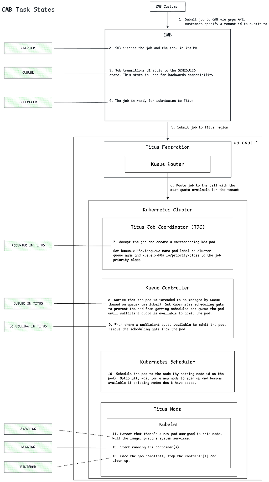
Netflix Batch User/Application Workload Submission Flow

The key difference between the old and new flows is that we defer queuing and scheduling to Kueue, which is enabled in each Kueue-enabled Titus cell. Titus federation routes the job to Kueue cells using our custom Kueue router.

Netflix Batch User/Application Tenant Management Flow

For us as operators, the migration was as simple as clicking a button on a tenant in our UI (as shown in the example above). This also allows us to easily rollback changes if there were issues.

Under the hood, this enrollment converts internal tenants to Cohorts and leaf tenants to a ClusterQueue + LocalQueue. The capacity configuration on a given tenant is converted into resource flavors and nominal quotas. The architecture for this looks as follows:

Lessons Learned

  1. Maintaining API parity with the existing system (vs exposing a new API surface) and migrating the underlying components as a first step derisked the project by unstacking bets while also ensuring we didn’t disrupt the customer experience.
  2. Don’t wait until the end to migrate the most complex use case. We decided early on to migrate our largest and most complex customer first. This allowed us to build confidence that we could later migrate other customers to Netflix Batch without issues, and resulted in the production migration lasting only 4 weeks.
  3. We had to run Kueue with much higher QPS, Burst, and groupKindConcurrency than the default configuration to meet our throughput needs. This was derisked early on by running load tests in a development environment that mimics Titus.

Current State of Kueue at Netflix

Kueue is fully rolled out in production, with it managing millions of batch workloads. In the future, we’re looking at options to enroll more of Titus batch workloads into this more managed experience. We have also productionized more fair sharing and preemptions to address better utilization of reserved capacity. In addition, our learnings are being leveraged by other internal teams, including those building Kubernetes-native training infrastructure, to inform their job scheduling and queuing configurations.

Fair Sharing and Preemption

With Kueue, Preemption-based Fair Sharing allows Netflix Batch to maintain reservation semantics while lending resources to other tenants when those reservations are not in use. In addition, preemption allows Netflix Batch to preempt lower-priority workloads for higher-priority workloads. For our customers, this means that tenants can use more idle capacity from reservations, submit more jobs without the risk of starvation, and have quicker turnaround times for business-critical workloads.

An example preemption configuration on a ClusterQueue that we would be using is as follows:

apiVersion: kueue.x-k8s.io/v1beta2
kind: ClusterQueue
metadata:
name: "team-a-cq"
spec:
preemption:
reclaimWithinCohort: Any
withinClusterQueue: LowerPriority

With these features deployed, Compute has seen a significant increase in average resource utilization.

Acknowledgement

This work would not have been possible without the great work of the entire Compute team at Netflix.


How Netflix Simplified Batch Compute with Kueue was originally published in Netflix TechBlog on Medium, where people are continuing the conversation by highlighting and responding to this story.

Palana (Part 2): Architecting isolation, identity, and auditability for AI agents

Post Syndicated from Grab Tech original https://engineering.grab.com/part-2-palana-architecture

Introduction

In Part 1, we introduced Palana, Grab’s Kubernetes-native secure execution platform for autonomous AI agents. We discussed the underlying need for isolated environments and covered its core design principles: treating isolation as the unit of trust, keeping credentials out of agent hands, and mediating all network access. In this second part, we’ll dive under the hood into Palana’s architecture, look at the agent lifecycle, and share the key lessons we learned from putting this system into production.

Architecture overview

The core request path looks like this:

Figure 1. Palana architecture overview.

The agent pod runs in a namespace owned by one user and one agent. It gets default-deny style network policy, domain name system (DNS), access to required platform services, and a persistent /data volume. Browser traffic enters through Traefik. LLM traffic goes to the LiteLLM wrapper in the gateway namespace. General Hypertext Transfer Protocol (HTTP) and Hypertext Transfer Protocol Secure (HTTPS) egress goes through the proxy namespace. Secrets are read from Vault only by the component authorized to use them.

The operator is responsible for turning a user request into the concrete Kubernetes shape:

  1. The user creates an agent through pcli (Palana command-line interface) or the portal.
  2. Palana writes a UserAgent or Agent custom resource with the raw user identity.
  3. The operator creates the user and agent namespaces, service accounts, role bindings, storage, network policies, and ingress.
  4. The user runs a template or container image.
  5. Admission webhooks inject proxy environment variables and enforce pod-level restrictions.
  6. Logs, policy decisions, and activity signals are emitted to observability systems.

Agent lifecycle

From a user’s perspective, the basic workflow is intentionally small:

./pcli login
./pcli create demo
./pcli secrets add demo GRABGPT_API_KEY token=<token>
./pcli run demo --template claudecodeui

Behind those commands, Palana provisions an isolated execution environment:

  • Namespace: agent-{sanitized-user}-{agent}
  • Service account: bound only to that namespace
  • Storage: an Amazon Elastic File System (EFS)-backed persistent volume claim (PVC) mounted at /data
  • Ingress: an agent-specific hostname protected by Concedo-backed browser auth
  • Egress: forced through platform proxies, except for approved internal platform services
  • Secrets: split between agent-readable and proxy-only Vault paths
  • Policies: proxy egress, network egress, and optional inter-agent peering rules

The same lifecycle is exposed in the portal for users who prefer a browser user interface (UI).

How Palana handles identity

Human authentication uses Concedo OpenID Connect (OIDC). pcli login performs a browser-based authorization code flow with Proof Key for Code Exchange (PKCE) and stores the resulting identity in an isolated kubeconfig. Browser access to agent UIs is protected by OAuth2-Proxy through Traefik forward auth.

The important detail is that Palana keeps the raw user identity, such as an email address, as the authoritative owner on the custom resource. That raw identity is used for Kubernetes role-based access control (RBAC) subject matching. Sanitized forms are used only where Kubernetes object names, labels, namespaces, or Vault paths require safer strings.

This split prevents a common class of identity bugs: the display-safe or path-safe version of a user ID should not accidentally become the authorization subject.

In the future, we will integrate Palana via SPIFFE (Secure Production Identity Framework for Everyone) and SPIRE (SPIFFE Runtime Environment) with the rest of our service mesh, to provide an agentic identity — a combination of user and agent instance id — that can then be controlled as a subset of a user’s capabilities. This gives us a first step into “agents on behalf of users” with cut-down permissions while the wider industry firms up the approaches via Open Authorization (OAuth) and other controls.

How Palana handles secrets

Palana’s Vault layout is designed around least privilege:

kv/agents/{user}/{agent}/{secret}
kv/proxy-secrets/{user}/{agent}/{secret}

The first path is for secrets the agent is allowed to read through its per-agent Vault role. The second path is for credentials the agent can use only through the proxy. For each proxy-only secret, Palana can create an agent-visible placeholder value. The placeholder is inert unless the request goes through the approved proxy path.

This gives teams a practical migration path. Existing clients can often be configured with a token-looking value, while Palana keeps the real token out of the runtime.

How Palana handles LLM access

LLM calls go through litellm-proxy-wrapper, which sits in front of LiteLLM and GrabGPT. The wrapper derives agent identity from Kubernetes context rather than trusting client-provided headers. It then looks up the per-agent GrabGPT credential in Vault and forwards the request to the correct upstream route.

The agent config uses internal base URLs such as:

http://litellm-proxy.gateway:4000/aws/v1
http://litellm-proxy.gateway:4000/unified/v1

That design gives us three useful properties:

  • Agents do not need raw upstream LLM credentials.
  • LLM traffic is attributable to a specific agent.
  • Provider routing and credential handling can evolve centrally.

How Palana handles network access

Network control is split into two layers.

At Layer 3 and Layer 4, Kubernetes NetworkPolicy and Cilium enforce which pods can talk to which namespaces, services, and classless inter-domain routing (CIDR) blocks. Agent namespaces are locked down to the platform paths they need: DNS, Vault, the egress proxy, the LLM gateway, and the Kubernetes application programming interface (API) patterns the platform explicitly supports.

At Layer 7, the proxy policy controls HTTP and HTTPS destinations by host, method, and agent identity. Open Policy Agent (OPA) evaluates per-agent policy. The proxy logs allow and deny decisions in structured form.

This split is deliberate. NetworkPolicy is good at containment. The proxy is good at application-aware decisions and audit. This allows us to be very expressive in the restrictions we place on our agents — by default, they get nothing; if they should have access to an internal service they get only that service, and cannot be used as an entry point to the wider internal environment.

Observability and operations

Palana treats observability as part of the safety model, not a nice-to-have. The platform emits structured logs for proxy decisions, Git activity, LLM requests, agent lifecycle, and idle-shutdown decisions. Operators can query activity by namespace, user, host, decision, or component.

One example is idle shutdown. Long-running agents are useful, but idle workloads consume cluster resources and expand the surface area that platform teams must monitor. Palana’s reaper records the most recent observable activity for each UserAgent. It combines signals from gateway/proxy logs, Git activity, Slack-routed agent messages, and Prometheus network activity. After a configurable idle threshold, it can warn the user and stop the workload while preserving /data, RBAC, namespace, and Vault state.

This is a good example of the platform philosophy: stop the compute, keep the state, and make resumption easy.

In addition, as we move into agentic operations, we use the many signals generated by Palana itself to aid our agents. For example, we have an agent that can monitor user workloads and provide advice and assistance if it spots issues — say, an agent is consistently out of memory (OOM), the ops agent can see that and message the user with instructions on how to increase the allocated memory. We don’t need to special-case every possible issue; instead we have agents that understand Palana logs and are able to communicate with the users themselves.

What we learned

Agent platforms need security controls at the platform layer

Prompt-level guardrails and model policies are useful, but they are not enough. Agents call tools, tools call services, and services use credentials. Palana puts controls where the action crosses a trust boundary: identity, egress, secrets, ingress, Git, and Kubernetes API access.

The user experience matters as much as the control

If the secure path requires every team to learn Terraform, Vault policy syntax, Kubernetes RBAC, and proxy configuration before they can try an agent, teams will work around it. Palana uses pcli, templates, and the portal to make the safe path the easy path.

Separating “can read a credential” from “can cause a credentialed request” is powerful

Proxy-only secrets are one of the highest-leverage design choices. They let agents perform authenticated work without turning the agent filesystem, logs, process environment, or prompt context into a credential store.

A namespace boundary is simple, but it compounds

Per-agent namespaces give us a consistent place to apply RBAC, storage, network policy, logging labels, resource quotas, and lifecycle controls. The pattern is easy to reason about during incidents: identify the namespace, identify the owner, inspect the policy, and isolate if needed.

Long-running agents need lifecycle management

Once agents persist for days or weeks, “run a container” becomes an incomplete product. Users need resume semantics. Operators need idle cleanup. Security teams need audit history. Platform teams need a way to rotate credentials, update images, and stop workloads externally.

What’s next

Palana is increasingly becoming a substrate for larger autonomous systems rather than only a place to run individual agents. Emerging patterns include:

  • Supervisor systems that route work to a pool of scoped agents.
  • Slack-native agents that wake up, handle a task, and scale back down.
  • Remote development environments backed by persistent cloud state.
  • Agent swarms where each worker has a separate namespace and credential scope.
  • Operational agents that investigate platform health and propose or apply small fixes under policy.
  • Security experiments around supply chain monitoring, token rotation, transport layer security (TLS) inspection, and automated isolation.

The north star is not “let every agent do anything”. It is to make useful autonomy boring to operate: attributable, inspectable, revocable, and recoverable.

Conclusion

AI agents are most valuable when they can act in real environments. That is also when they become risky. Palana gives Grab a way to keep both sides of that tradeoff in view: teams can move quickly with self-service agent environments, while the platform keeps isolation, identity, secrets, network access, and auditability as defaults.

We expect the underlying tools and models to keep changing. The platform primitives are more durable. Agents will vary, but they will still need a place to run, a way to authenticate, a boundary around their actions, and a record of what happened.

That is the role Palana is designed to play.

Join us

Grab is Southeast Asia’s leading superapp, serving over 900 cities across eight countries (Cambodia, Indonesia, Malaysia, Myanmar, the Philippines, Singapore, Thailand, and Vietnam). Through a single platform, millions of users access mobility, delivery, and digital financial services, including ride-hailing, food delivery, payments, lending, and digital banking via GXS Bank and GXBank. Founded in 2012, Grab’s mission is to drive Southeast Asia forward by creating economic empowerment for everyone while delivering sustainable financial performance and positive social impact.

Powered by technology and driven by heart, our mission is to drive Southeast Asia forward by creating economic empowerment for everyone. If this mission speaks to you, join our team today!
Palana (Part 1): Why Grab built a secure platform for autonomous AI Agents

Post Syndicated from Grab Tech original https://engineering.grab.com/palana-part-1-secure-platform-for-ai-agents

Abstract

Artificial intelligence (AI) agents are moving from experiments into everyday engineering workflows. They can read code, call application programming interfaces (APIs), run tests, create merge requests, answer Slack messages, and keep long-running state. That makes them useful, but it also changes the risk model – especially as agents get more autonomous in their use of tools. An agent with network access, credentials, tools, and memory is no longer just a chat interface. It is a workload that can act.

The more capability we give to the agents, the more valuable they get – but they also get riskier, and maintaining controls and oversight gets more challenging. We need isolated environments, with clear intentional capabilities added rather than just inheriting “everything on your laptop”.

Palana is Grab’s Kubernetes-native platform for running those workloads safely. It gives each agent an isolated namespace, persistent storage, controlled ingress, proxy-mediated egress, Vault-backed credential injection, large language model (LLM) routing, Git access controls, structured audit logs, and emergency kill switches. It is currently used to run hundreds of agents, including remote development environments, Slack automation, OpenClaw workers, Hermes agents, and other long-running internal systems.

In this post, we share why we built Palana, what it does, and how its architecture lets teams experiment with autonomous agents without giving up control over identity, secrets, network access, and operational visibility.

Introduction

The first wave of AI coding tools lived close to the user: an integrated development environment (IDE) plugin, a chat window, or a command-line assistant running on a developer’s laptop. That model is familiar and easy to adopt, but it has limits. Long-running agents need persistent state. Team workflows need shared access through Slack or web user interfaces (UIs). Security teams need to inspect what an agent is doing, and apply highly granular controls over what an agent can do. Platform teams need a way to stop, resume, update, and audit the workload.

As usage grew, we started seeing the same question in different forms:

How do we let agents do useful work inside the company without treating every new agent as a bespoke infrastructure project?

The answer was not simply to “run agents in containers”. Containers help package the runtime, but they do not answer the harder platform questions:

  • Which user does this agent act on behalf of?
  • What credentials can it use?
  • Can it see another user’s state?
  • Can it connect directly to the internet?
  • How do we inspect LLM, Git, and Hypertext Transfer Protocol (HTTP) activity after something goes wrong?
  • How do we stop an agent quickly without trusting the agent to cooperate?
  • How do we give teams a self-service experience without handing them cluster-admin access?

Palana is our answer to those questions.

What Palana is

Palana, an in-house proprietary system built by the CyberSecurity team at Grab, is a secure execution substrate for autonomous and semi-autonomous agents. The name comes from a Sanskrit root associated with protection, maintenance, and care. That maps well to the platform’s purpose: Palana is not trying to be the agent’s brain. It is the environment that contains, observes, and sustains the agent while it works.

At a high level, Palana provides:

  • A Kubernetes namespace per agent, with role-based access control (RBAC), resource quotas, network policy, and storage scoped to that agent.
  • A command-line and portal experience for creating, running, stopping, configuring, and inspecting agents.
  • Persistent /data storage so long-running agents can preserve memory, caches, repositories, and session state across restarts.
  • Browser and shell access for interactive workloads such as Claude Code UI, OpenCode, IDEs, ttyd, or Secure Shell (SSH)-backed development flows.
  • LLM access through a LiteLLM wrapper that injects per-agent GrabGPT credentials from Vault.
  • HTTP and HTTPS egress through an Envoy and ext-authz proxy path, with Open Policy Agent (OPA) policy checks and structured request logs.
  • Proxy-only secrets, where agents can reference placeholder tokens but cannot read the underlying credentials directly.
  • Git access through a bastion path so repository operations are attributable and policy-controlled.
  • Kill switches and idle shutdown so the control plane can isolate or stop workloads from outside the agent process.

This combination lets Palana support several categories of work:

  • Secure OpenClaw and agent-framework testing.
  • Cloud development environments accessible from a browser or SSH client.
  • Fast prototyping and testing for agentic workloads in a secure environment.
  • Slack-connected agents such as cts-aergia and Claude-to-Slack workflows.
  • Long-running task agents such as Hermes, Matlock, Butler, and custom team automations.
  • Higher-order systems where agentic supervisors launch or route work to scoped agents.

Why we built it

The immediate need came from security research. We wanted a place to run and investigate OpenClaw and related agent frameworks without exposing the broader internal network or placing raw credentials inside the agent runtime. That use case forced us to design for containment from the beginning.

The broader need quickly became developer productivity. Once the basic primitives existed, Palana became useful for remote coding, Slack automation, internal assistants, long-lived experiments, and agentic operational workflows. Grabbers wanted agents that could keep context over days or weeks, run from corporate infrastructure, access approved internal services, and survive laptop sleep, local dependency drift, or network changes.

The security and productivity goals reinforce each other. If the safe path is self-service and ergonomic, teams are more likely to use it. If the productive path is observable and policy-controlled by default, and the appropriate security is baked into the system automatically, platform teams do not have to retrofit controls after adoption.

Design principles

Palana’s architecture follows a few principles that shaped most of the implementation.

Isolation is the unit of trust

Each agent gets its own namespace, service account, storage, network policy, and Vault scope. Agents should not see each other’s pods, secrets, or filesystem state by default. Inter-agent communication is possible, but it goes through explicit peering rules rather than ambient pod-to-pod reachability.

This means the platform does not have to assume every agent framework has perfect multi-tenant isolation internally. A framework designed as a single-user assistant can still be hosted safely by giving each user or worker its own Palana boundary.

Credentials are never given to the agent

Traditional application hosting often gives credentials to the workload as environment variables or mounted files. That is risky for agent workloads because the agent may execute tools, run untrusted code, summarize files, install packages, or expose a web UI.

Palana separates two kinds of secrets:

  • Agent-readable secrets live under the agent’s own Vault path and are available only to that agent’s service account.
  • Proxy-only secrets are stored under a separate Vault path and are read by the proxy layer, not by the agent.

For proxy-only secrets, the agent sees a placeholder such as TOKEN_GITHUB_PAT or TOKEN_GRABGPT_API_KEY. When an outbound request travels through the proxy path, the proxy replaces the placeholder header with the real credential from Vault. The remote service receives a valid token, but the agent process never stores the token in its own environment or config.

This pattern is especially important for LLMs, source control, API integrations, and browser-like tools where prompt injection or dependency compromise could otherwise expose long-lived credentials.

Egress is a control point

Agents can be useful only if they can call tools and services. Instead of forbidding network access, Palana makes network access observable and policy-mediated.

Agent pods receive proxy configuration automatically. External HTTP and HTTPS traffic flows through Envoy. Envoy asks ext-authz-proxy to identify the calling pod, evaluate policy with OPA, log the request, and optionally inject credentials. HTTPS traffic can be terminated by the proxy’s man-in-the-middle (MITM) listener for header inspection and replacement, with the generated certificate authority (CA) distributed to agent pods.

This gives the platform a place to answer questions that normal Kubernetes networking cannot answer alone:

  • Which agent made this request?
  • Which user owns that agent?
  • Which host and method were requested?
  • Was the request allowed or denied?
  • Which placeholder credentials were replaced?
  • Did the request go to an internal service, an LLM gateway, GitLab, or the public internet?

The control plane must stay outside the agent

Palana assumes an agent might become confused, compromised, or uncooperative. Operational controls therefore live outside the agent process. The operator reconciles namespaces and policies. The proxy controls egress. The portal and pcli (Palana command-line interface) manage lifecycle. The kill switch is enforced with network policy. Idle shutdown is handled by a separate reaper CronJob.

That separation matters. A kill switch that asks the agent to stop is a feature. A kill switch that removes the agent’s network path is a safety control.

Use Kubernetes primitives where they fit

Palana is intentionally Kubernetes-native. Agents are represented by custom resources. The operator reconciles namespaces, RBAC, storage, services, ingress, and network policies. Users can interact through pcli or the portal, while platform engineers can still inspect the underlying Kubernetes objects when debugging.

This gives us a layered experience: simple workflows for users, direct primitives for advanced operators, and infrastructure-as-code for the deployed platform.

Conclusion

By centering the design around isolation, controlled egress, and proxy-mediated secrets, Palana provides a secure foundation for AI agents to operate within Grab. In Part 2, we will dive deeper into the under-the-hood architecture of Palana, exploring how it orchestrates agent lifecycles, handles LLM routing, and maintains operational visibility.

Join us

Grab is Southeast Asia’s leading superapp, serving over 900 cities across eight countries (Cambodia, Indonesia, Malaysia, Myanmar, the Philippines, Singapore, Thailand, and Vietnam). Through a single platform, millions of users access mobility, delivery, and digital financial services, including ride-hailing, food delivery, payments, lending, and digital banking via GXS Bank and GXBank. Founded in 2012, Grab’s mission is to drive Southeast Asia forward by creating economic empowerment for everyone while delivering sustainable financial performance and positive social impact.

Powered by technology and driven by heart, our mission is to drive Southeast Asia forward by creating economic empowerment for everyone. If this mission speaks to you, join our team today!
Diagnose EKS Node Issues Faster with AWS DevOps Agent and Custom MCP

Post Syndicated from Shyam Kulkarni original https://aws.amazon.com/blogs/devops/diagnose-eks-node-issues-faster-with-aws-devops-agent-and-custom-mcp/

AWS DevOps Agent can investigate a growing range of production incidents autonomously. It diagnoses CrashLoopBackOff failures, traces ConfigMap deletions through audit logs, and correlates Amazon CloudWatch metrics with cluster events — all without human intervention.

But AWS DevOps Agent has a visibility boundary. When the data it needs lives outside its native integrations — on a node’s operating system, inside a third-party monitoring tool, behind a database’s internal diagnostics — the agent stalls. It can describe symptoms, but it can’t reach the evidence needed to identify root causes.

This post shows how to extend AWS DevOps Agent by building a custom Model Context Protocol (MCP) server that bridges that gap. Using a concrete example, we give AWS DevOps Agent structured access to Amazon EKS worker node diagnostics and explain how the same approach applies to data sources the agent can’t natively reach. By the end of this walkthrough, you will have a working MCP server that gives AWS DevOps Agent access to 20+ node-level log sources — providing autonomous investigation capabilities that can assist in root cause analysis compared to manual SSH sessions.

Prerequisites

Before you begin, make sure you have the following:

  • An Amazon EKS cluster with AWS Systems Manager Agent (SSM Agent) running on the worker nodes (included by default on Amazon EKS optimized AMIs)
  • Node.js v18 or later
  • AWS CLI v2
  • AWS CDK v2 installed and bootstrapped in your target account and Region
  • An AWS account with permissions to create IAM roles, Lambda functions, and Amazon S3 buckets
  • Familiarity with Amazon EKS, AWS Systems Manager, and the Model Context Protocol (MCP)

How AWS DevOps Agent discovers custom tools through MCP

MCP is an open standard that defines how AI agents discover and invoke external tools. AWS DevOps Agent supports connecting to custom MCP servers, which means you can expose new capabilities to it without modifying the agent itself. When you connect an MCP server to AWS DevOps Agent, the agent automatically discovers the available tools, understands their schemas, and calls them as part of its investigation workflow. You build and connect the MCP server — the agent handles the rest.

The extensibility model follows three steps: first, identify the data source that AWS DevOps Agent cannot natively access; second, build an MCP server that wraps safe, structured access to that data source; and third, connect the MCP server to AWS DevOps Agent so it can incorporate the new tools into its investigations.

Three design principles make this work. Return structured data, not raw text — pre-index findings with severity levels and stable IDs so the agent can filter, reference, and correlate them. Never give the agent a shell — mediate interactions through a controlled, auditable execution model. Make tools composable — design tool outputs to serve as inputs to other tools, creating a chain of evidence the agent can follow.

Why Amazon EKS node OS visibility matters

AWS DevOps Agent integrates with Amazon EKS to inspect pod status, read container logs, query CloudWatch Container Insights, and correlate cluster events. This covers application crashes, container-level resource exhaustion, and configuration drift.

However, EKS production issues with nodes originate in a layer these tools cannot reach: the node operating system. Artifacts such as iptables rules, full CNI configuration and IPAMD state, route tables, conntrack entries, dmesg kernel messages, containerd runtime logs, sysctl parameters, ENI metadata, and the unfiltered kubelet journal exist exclusively on the node. These artifacts are the primary evidence for diagnosing IP allocation failures, DNS resolution issues, network policy enforcement problems, storage mount timeouts, and node registration failures.

Integrating AWS DevOps Agent with an EKS node diagnostics MCP server

The sample-eks-node-diagnostics-mcp repository (sample-eks-node-diagnostics-mcp repository) demonstrates this pattern. It provides an MCP server that gives AWS DevOps Agent structured access to node-level diagnostic data, backed by AWS Systems Manager (SSM) Automation for safe, auditable execution.

How it works

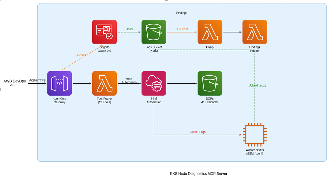
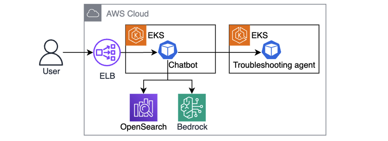
AWS DevOps Agent connects over MCP/HTTPS to AgentCore Gateway, which authenticates via Amazon Cognito OAuth 2.0 and routes tool calls through a Lambda-based Tool Router to SSM Automation. SSM Automation dispatches runbooks to EKS worker nodes running SSM Agent, which upload collected log archives to a KMS-encrypted S3 bucket. An S3 event triggers a Lambda function that extracts and indexes findings for the agent to query.

Figure 1: End-to-end architecture of the EKS Node Diagnostics MCP server. AWS DevOps Agent discovers and invokes 19 tools through AgentCore Gateway, which dispatches SSM Automation runbooks to worker nodes for log collection and uploads results to Amazon S3 for extraction and indexing.

  1. AWS DevOps Agent calls a collect tool with an instance ID.
  2. The MCP server dispatches an SSM Automation execution to the target node, running the AWS-managed AWSSupport-CollectEKSInstanceLogs runbook.
  3. The runbook collects 20+ log sources — kubelet, containerd, iptables, CNI config, route tables, dmesg, sysctl, ENI metadata, IPAMD logs, and more — packages them into an archive, and uploads it to an Amazon S3 bucket where you configure AWS KMS encryption.
  4. A processing pipeline extracts the archive, pre-indexes errors with severity classification and stable finding IDs, and provides the results to you through additional MCP tools.

The server exposes tools for log collection, pre-indexed error retrieval, cross-file search and correlation, structured network diagnostics, and live packet capture. A typical agent workflow chains these together: collect → status → errors → search → correlate → read → summarize, with each step producing outputs that feed into the next.

AWS DevOps Agent does not get a shell on the node. Every interaction is mediated by SSM Automation — an auditable, IAM-controlled, non-interactive execution model.

Connecting through Amazon Bedrock AgentCore Gateway

The reference implementation uses Amazon Bedrock AgentCore Gateway to expose the Lambda-backed MCP server to AWS DevOps Agent. AgentCore Gateway converts Lambda functions into MCP-compatible tools and handles authentication, protocol translation, and tool discovery through a single managed endpoint.

The integration follows three steps:

Step 1: Create an OAuth authorizer with Amazon Cognito. The CDK stack provisions a Cognito User Pool configured for the OAuth 2.0 client credentials flow. This secures inbound access to the gateway — only clients with valid tokens can invoke tools.

Step 2: Create a gateway and register the Lambda as a target. Register the Lambda function that handles tool invocations as a target on the gateway. AgentCore Gateway automatically discovers the tool schemas from the Lambda and makes them available through the MCP protocol. The gateway endpoint becomes the single MCP URL for AWS DevOps Agent.

Step 3: Connect AWS DevOps Agent. Register the MCP server at the account level in the AWS DevOps Agent console, providing the gateway URL and OAuth configuration. Then allowlist the specific tools each Agent Space needs. AWS DevOps Agent authenticates by obtaining a JWT from the Cognito token endpoint using the client credentials grant and passes it as a Bearer token in requests to the gateway URL.

Deploying the MCP server

Deploy the entire stack using AWS CDK :

git clone https://github.com/aws-samples/sample-eks-node-diagnostics-mcp.git
 cd sample-eks-node-diagnostics-mcp
 chmod +x deploy.sh
 ./deploy.sh

The script walks you through cluster selection and node role configuration. Have the following ready before running the script: your target EKS cluster name, the IAM role ARN you attached to your worker nodes, and the AWS Region where your cluster runs. The script outputs your MCP gateway URL, OAuth credentials, and token endpoint — everything you need to configure the connection in AWS DevOps Agent. See the repository README for detailed deployment instructions, CI/CD mode, and prerequisite details.

Seeing it in action

To demonstrate the MCP server’s capabilities, we walk through a realistic node-level failure scenario on a test EKS cluster. We manually inject a fault that blocks pod DNS resolution at the iptables level — an issue that is invisible from kubectl since pods appear Running — then show how AWS DevOps Agent investigates and identifies the root cause using the MCP server’s tools.

Setting up the scenario

Start with an EKS cluster that has a managed node group with SSM Agent running (included by default on Amazon EKS optimized AMIs). Deploy a sample workload to one of the nodes:

kubectl create namespace demo-app

cat <<EOF | kubectl apply -f -
 apiVersion: apps/v1
 kind: Deployment
 metadata:
   name: web-frontend
   namespace: demo-app
 spec:
   replicas: 3
   selector:
     matchLabels:
       app: web-frontend
   template:
     metadata:
       labels:
         app: web-frontend
     spec:
       containers:
       - name: nginx
         image: nginx:latest
         ports:
         - containerPort: 80
 EOF

Identify the node and instance ID where the pods are running:

kubectl get pods -n demo-app -o wide

Injecting the fault

⚠ WARNING: The following commands will disrupt DNS resolution for all pods on the target node. Only run these in a non-production test environment. Do not execute on production nodes.

Connect to the target node using SSM Session Manager and run the following commands to block pod DNS traffic at the iptables level. This simulates a subtle networking issue – pods continue running but can’t resolve DNS, and the root cause is only visible in the node’s iptables rules:

# Block pod traffic to kube-dns ClusterIP — pods run but DNS fails
 # Only affects FORWARD chain (pod traffic), not the node's own DNS
 sudo iptables -I FORWARD -d 10.100.0.10/32 -p udp --dport 53 -j DROP
 sudo iptables -I FORWARD -d 10.100.0.10/32 -p tcp --dport 53 -j DROP

Replace 10.100.0.10 with your cluster’s kube-dns ClusterIP (kubectl get svc kube-dns -n kube-system -o jsonpath=’{.spec.clusterIP}’).

This fault is particularly insidious because kubectl get pods shows all pods in Running state. The applications fail with DNS resolution errors, but there is no Kubernetes event or pod status that points to the cause. The iptables DROP rules targeting the kube-dns ClusterIP exist only in the node’s firewall configuration — a layer that no Kubernetes API call can inspect.

Investigating with AWS DevOps Agent

An engineer notices applications reporting DNS failures and asks AWS DevOps Agent to investigate:

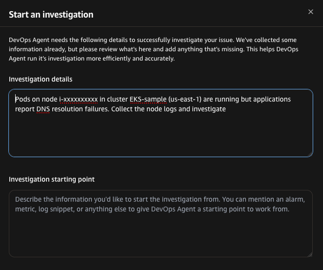
“Pods on node i-xxxxxxxxxx in cluster EKS-sample (us-east-1) are running but applications report DNS resolution failures. Collect the node logs and investigate.”

The AWS DevOps Agent "Start an investigation" dialog with the investigation details field populated: "Pods on node i-xxxxxxxxxxxx in cluster EKS-sample (us-east-1) are running but applications report DNS resolution failures. Collect the node logs and investigate." The date and time of incident is set to 2026-03-26T16:55:30.593Z.

Figure 2: Starting an investigation in AWS DevOps Agent. The engineer provides the symptom description and incident timestamp, and the agent autonomously plans and executes the investigation.

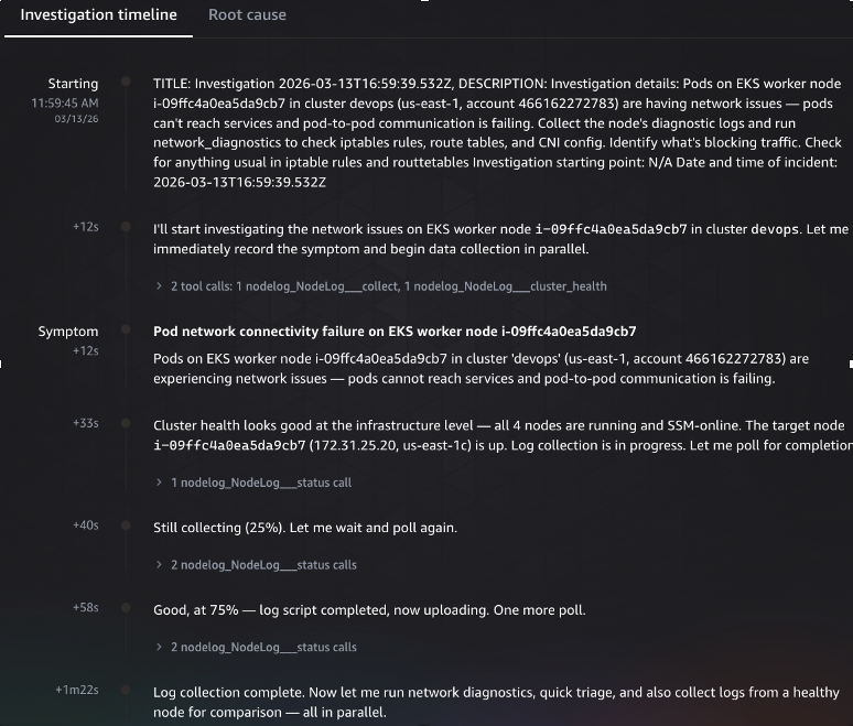
AWS DevOps Agent begins the investigation by recording the symptom and launching two parallel actions: collecting node logs via the nodelog_collect tool and checking cluster health. The cluster health check confirms all four nodes are running and SSM-online. The agent then polls the log collection status, tracking progress from 25% through 75% to completion. Once collection finishes, the agent fans out into parallel workstreams — running network diagnostics, performing quick triage, and collecting logs from a healthy node for comparison.

The investigation timeline progresses from "Starting" at 11:59:45 AM through symptom identification at +12 seconds, cluster health check at +33 seconds confirming all four nodes are running, log collection polling at 25% and 75%, to log collection complete at +1 minute 22 seconds. The agent then launches parallel network diagnostics, quick triage, and healthy node comparison.

Figure 3: Investigation timeline showing the initial data collection phase. The agent identifies the symptom, confirms cluster health, collects node logs via SSM Automation, polls for completion, and launches parallel diagnostic workstreams.

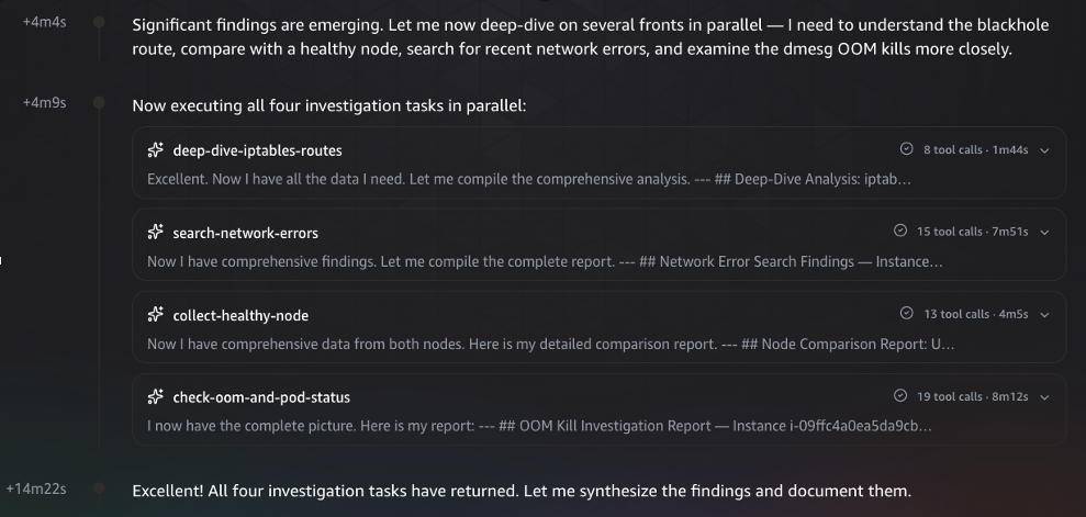
With the initial data collected, the agent launches four parallel investigation tasks to maximize coverage and minimize time-to-root-cause: (1) deep-dive-iptables-routes examines the node’s firewall rules and routing table in detail, completing in 1 minute 44 seconds across 8 tool calls; (2) search-network-errors scans the collected logs for network-related error patterns, running 15 tool calls over 7 minutes 51 seconds; (3) collect-healthy-node gathers the same diagnostics from a known-good node for comparison, taking 13 tool calls over 4 minutes 55 seconds; (4) check-oom-and-pod-status investigates kernel OOM kills and pod health, executing 19 tool calls over 8 minutes 12 seconds. Each task produces a structured report that feeds into the final synthesis.

Four parallel investigation tasks execute concurrently: deep-dive-iptables-routes (8 tool calls, 1 minute 44 seconds), search-network-errors (15 tool calls, 7 minutes 51 seconds), collect-healthy-node (13 tool calls, 4 minutes 5 seconds), and check-oom-and-pod-status (19 tool calls, 8 minutes 12 seconds). At +14 minutes 22 seconds, all four tasks complete and the agent begins synthesizing findings.

Figure 4: Parallel investigation phase. The agent runs four concurrent deep-dive tasks — iptables/route analysis, network error search, healthy node comparison, and OOM/pod status check — then synthesizes the findings into a unified report.

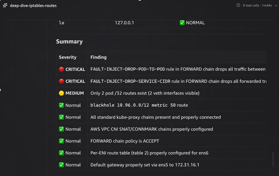
The iptables and route table deep-dive reveals the root cause. The agent identifies two CRITICAL findings: a FAULT-INJECT-DROP-POD-TO-POD rule in the FORWARD chain that drops inter-pod traffic, and a FAULT-INJECT-DROP-SERVICE-CIDR rule that drops forwarded traffic to the service CIDR range. It also flags a MEDIUM-severity finding — a blackhole route for 10.96.0.0/12 (the Kubernetes service CIDR) that does not exist on healthy nodes. The remaining checks come back normal: kube-proxy chains are intact, AWS VPC CNI SNAT/CONNMARK chains are properly configured, and the default gateway and ENI route tables are correct. This structured severity classification allows the agent to immediately focus on the critical items.

A severity-classified findings summary table from the deep-dive-iptables-routes task. Two CRITICAL findings: a FAULT-INJECT-DROP-POD-TO-POD rule and a FAULT-INJECT-DROP-SERVICE-CIDR rule, both in the FORWARD chain. One MEDIUM finding about limited pod /32 routes. Six Normal findings confirm kube-proxy chains, AWS VPC CNI SNAT/CONNMARK chains, FORWARD chain policy, per-ENI route table, and default gateway are all properly configured.

Figure 5: Deep-dive findings from the iptables and route table analysis. Two CRITICAL fault-injection DROP rules in the FORWARD chain are identified as the primary issue, while standard networking components — kube-proxy, VPC CNI, and routing — check normal.

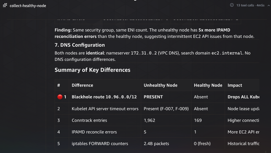
The healthy node comparison confirms the diagnosis. The agent compares the unhealthy node against a known-good node across seven dimensions: security groups, ENI count, DNS configuration, iptables rules, route tables, conntrack entries, and IPAMD state. The key differences are definitive: the blackhole route for 10.96.0.0/12 exists only on the unhealthy node, kubelet API server timeout errors appear only on the unhealthy node, conntrack entries are 12x higher (1,962 vs 169), and IPAMD reconciliation errors are 5x more frequent. The iptables FORWARD chain counters show 2.4 billion packets processed on the unhealthy node versus zero on the freshly-started healthy node — confirming sustained traffic disruption.

A comparison table titled "Summary of Key Differences" between the unhealthy and healthy nodes. Five differences are listed: a blackhole route for 10.96.0.0/12 present only on the unhealthy node, kubelet API server timeout errors present only on the unhealthy node, conntrack entries at 1,962 versus 169, IPAMD reconcile errors at 5 versus 1, and iptables FORWARD counters at 2.4 billion packets versus 0 on the fresh healthy node. DNS configuration is identical on both nodes.

Figure 6: Healthy node comparison confirming the diagnosis. The agent compares diagnostics across both nodes and identifies five key differences — the blackhole route, elevated conntrack entries, and high FORWARD chain packet counts exist only on the affected node.

The agent synthesizes the findings into a definitive root cause determination. It identifies a fault-injection namespace on the EKS cluster that is running chaos experiments, introducing three specific network-disrupting modifications on the target node: (1) a FAULT-INJECT-DROP-POD-TO-POD iptables rule in the FORWARD chain that drops inter-pod traffic, (2) a FAULT-INJECT-DROP-SERVICE-CIDR rule that drops forwarded traffic to the Kubernetes service CIDR, and (3) a blackhole route for 10.96.0.0/12 that does not exist on healthy nodes. Together, these three modifications create a multi-vector network disruption — pods appear Running but cannot communicate with each other or reach Kubernetes services, including kube-dns.

The Root causes panel identifies one root cause: "Fault-injection workloads on node i-09ffc4a0ea5da9cb7 causing multi-vector network disruption." The explanation states that a fault-injection namespace is running chaos experiments that introduced two iptables FORWARD chain DROP rules (FAULT-INJECT-DROP-POD-TO-POD and FAULT-INJECT-DROP-SERVICE-CIDR) and a blackhole route for 10.96.0.0/12 that does not exist on healthy nodes.

Figure 7: Root cause determination. The agent traces the multi-vector network disruption to three fault-injection modifications — two iptables DROP rules and a blackhole route — deployed by a chaos experiment namespace on the target node.

Cleaning up the fault

To restore the node after the demo, connect via SSM Session Manager and run:

sudo iptables -D FORWARD -d 10.100.0.10/32 -p udp --dport 53 -j DROP
sudo iptables -D FORWARD -d 10.100.0.10/32 -p tcp --dport 53 -j DROP

Extending this pattern to other data sources

The EKS node diagnostics use case demonstrates the pattern, but the architecture generalizes to systems where the SSM Agent is running and you can define an SSM Automation runbook to collect the data you need.

For example, an EC2 instance with SSM Agent can use this same approach — collect OS-level logs, network configuration, package state, or application diagnostics through a custom or pre-built SSM Automation runbook, upload results to S3, and expose them through MCP tools. The same applies to ECS container instances (Docker daemon logs, ECS agent state, iptables), on-premises servers registered via SSM Hybrid Activations, or managed nodes in your fleet.

The pattern also extends beyond SSM-managed hosts. Network devices can be reached through API calls to their management planes, databases through read-only diagnostic queries, and third-party APM tools through vendor API integrations. In each case, the same three-step approach holds: identify the unreachable data, build an MCP server that wraps safe access to it, and connect it to AWS DevOps Agent.

When to use this approach
This pattern works well for incident response where diagnostic data lives outside AWS DevOps Agent’s native reach, fleet-wide triage where manual access to individual systems is impractical, and cross-source correlation where evidence spans multiple log sources.

It is not a replacement for continuous monitoring (use CloudWatch Container Insights or Prometheus for real-time alerting), log shipping (if you have compliance requirements for continuous retention), or native integrations where the agent already has access to the data source.

The reference implementation requires SSM Agent running on the nodes with appropriate IAM permissions. It is a proof of concept — validate it in non-production environments before using it with production workloads.

Clean up

Cost considerations: This solution uses AWS Lambda, Amazon S3, AWS KMS, Amazon Cognito, and Amazon Bedrock AgentCore Gateway. Costs vary based on usage. Lambda charges apply per invocation and duration. S3 charges apply for log storage. KMS charges a per-key monthly fee plus per-request charges. Cognito charges per monthly active user. AgentCore Gateway pricing is based on API calls. For current pricing details, see the AWS Pricing page for each service. To minimize costs during evaluation, delete the stack when not in use.

Remove the deployed resources by running cdk destroy from the repository root. The S3 log bucket uses a RETAIN removal policy — delete it manually after stack destruction if needed.

Conclusion

MCP provides a standardized extensibility mechanism that lets you bridge visibility gaps in AWS DevOps Agent without modifying the agent itself. The pattern is straightforward: identify the unreachable data source, build an MCP server that wraps safe and structured access to it, and connect it to AWS DevOps Agent through Amazon Bedrock AgentCore Gateway. The agent handles the reasoning. The MCP server handles the data access.

To get started:

  • Deploy the reference implementation (sample-eks-node-diagnostics-mcp repository) in a non-production environment.
  • Review the MCP specification (MCP specification).
  • Explore the Amazon EKS troubleshooting documentation (Amazon EKS troubleshooting documentation).
  • Connect custom MCP servers to AWS DevOps Agent — see the Connecting MCP Servers guide in the AWS DevOps Agent documentation.
  • Set up AgentCore Gateway — see the Amazon Bedrock AgentCore Gateway quick start guide.

About the author

Shyam Kulkarni

Shyam Kulkarni

Shyam Kulkarni is a Sr. Technical Account Manager at AWS, where he helps enterprise customers design and implement cloud-native architectures with a focus on container orchestration, platform engineering, and observability at scale. He advises organizations on strategic modernization initiatives and is passionate about architecting AI-native systems, including agentic AI platforms and scalable AI infrastructure. Outside of work, Shyam is an avid travel and landscape photographer who enjoys exploring new destinations and capturing dramatic natural scenery. He’s also an enthusiastic home cook and baker who loves experimenting with new recipes, flavors, and techniques in the kitchen. When not behind a camera or in the kitchen, you’ll find him hiking remote trails.

A one-line Kubernetes fix that saved 600 hours a year

Post Syndicated from Braxton Schafer original https://blog.cloudflare.com/one-line-kubernetes-fix-saved-600-hours-a-year/

Every time we restarted Atlantis, the tool we use to plan and apply Terraform changes, we’d be stuck for 30 minutes waiting for it to come back up. No plans, no applies, no infrastructure changes for any repository managed by Atlantis. With roughly 100 restarts a month for credential rotations and unboarding, that added up to over 50 hours of blocked engineering time every month, and paged the on-call engineer every time.

This was ultimately caused by a safe default in Kubernetes that had silently become a bottleneck as the persistent volume used by Atlantis grew to millions of files. Here’s how we tracked it down and fixed it with a one-line change.

Mysteriously slow restarts

We manage dozens of Terraform projects with GitLab merge requests (MRs) using Atlantis, which handles planning and applying. It enforces locking to ensure that only one MR can modify a project at a time. 

It runs on Kubernetes as a singleton StatefulSet and relies on a Kubernetes PersistentVolume (PV) to keep track of repository state on disk. Whenever a Terraform project needs to be onboarded or offboarded, or credentials used by Terraform are updated, we have to restart Atlantis to pick up those changes — a process that can take 30 minutes.

The slow restart was apparent when we recently ran out of inodes on the persistent storage used by Atlantis, forcing us to restart it to resize the volume. Inodes are consumed by each file and directory entry on disk, and the number available to a filesystem is determined by parameters passed when creating it. The Ceph persistent storage implementation provided by our Kubernetes platform does not expose a way to pass flags to mkfs, so we’re at the mercy of default values: growing the filesystem is the only way to grow available inodes, and restarting a PV requires a pod restart. 

We talked about extending the alert window, but that would just mask the problem and delay our response to actual issues. Instead, we decided to investigate exactly why it was taking so long.

Bad behavior

When we were asked to do a rolling restart of Atlantis to pick up a change to the secrets it uses, we would run kubectl rollout restart statefulset atlantis, which would gracefully terminate the existing Atlantis pod before spinning up a new one. The new pod would appear almost immediately, but looking at it would show:

$ kubectl get pod atlantis-0
atlantis-0                                                        0/1     
Init:0/1     0             30m

…so what gives? Naturally, the first thing to check would be events for that pod. It’s waiting around for an init container to run, so maybe the pod events would illuminate why?

$ kubectl events --for=pod/atlantis-0
LAST SEEN   TYPE      REASON                   OBJECT                   MESSAGE
30m         Normal    Killing                  Pod/atlantis-0   Stopping container atlantis-server
30m        Normal    Scheduled                Pod/atlantis-0   Successfully assigned atlantis/atlantis-0 to 36com1167.cfops.net
22s         Normal    Pulling                  Pod/atlantis-0   Pulling image "oci.example.com/git-sync/master:v4.1.0"
22s         Normal    Pulled                   Pod/atlantis-0   Successfully pulled image "oci.example.com/git-sync/master:v4.1.0" in 632ms (632ms including waiting). Image size: 58518579 bytes.

That looks almost normal… but what’s taking so long between scheduling the pod and actually starting to pull the image for the init container? Unfortunately that was all the data we had to go on from Kubernetes itself. But surely there had to be something more that can tell us why it’s taking so long to actually start running the pod.

Going deeper

In Kubernetes, a component called kubelet that runs on each node is responsible for coordinating pod creation, mounting persistent volumes, and many other things. From my time on our Kubernetes team, I know that kubelet runs as a systemd service and so its logs should be available to us in Kibana. Since the pod has been scheduled, we know the host name we’re interested in, and the log messages from kubelet include the associated object, so we could filter for atlantis to narrow down the log messages to anything we found interesting.

We were able to observe the Atlantis PV being mounted shortly after the pod was scheduled. We also observed all the secret volumes mount without issue. However, there was still a big unexplained gap in the logs. We saw:

[operation_generator.go:664] "MountVolume.MountDevice succeeded for volume \"pvc-94b75052-8d70-4c67-993a-9238613f3b99\" (UniqueName: \"kubernetes.io/csi/rook-ceph-nvme.rbd.csi.ceph.com^0001-000e-rook-ceph-nvme-0000000000000002-a6163184-670f-422b-a135-a1246dba4695\") pod \"atlantis-0\" (UID: \"83089f13-2d9b-46ed-a4d3-cba885f9f48a\") device mount path \"/state/var/lib/kubelet/plugins/kubernetes.io/csi/rook-ceph-nvme.rbd.csi.ceph.com/d42dcb508f87fa241a49c4f589c03d80de2f720a87e36932aedc4c07840e2dfc/globalmount\"" pod="atlantis/atlantis-0"
[pod_workers.go:1298] "Error syncing pod, skipping" err="unmounted volumes=[atlantis-storage], unattached volumes=[], failed to process volumes=[]: context deadline exceeded" pod="atlantis/atlantis-0" podUID="83089f13-2d9b-46ed-a4d3-cba885f9f48a"
[util.go:30] "No sandbox for pod can be found. Need to start a new one" pod="atlantis/atlantis-0"

The last two messages looped several times until eventually we observed the pod actually start up properly.

So kubelet thinks that the pod is otherwise ready to go, but it’s not starting it and something’s timing out.

The missing piece

The lowest-level logs we had on the pod didn’t show us what’s going on. What else do we have to look at? Well, the last message before it hangs is the PV being mounted onto the node. Ordinarily, if the PV has issues mounting (e.g. due to still being stuck mounted on another node), that will bubble up as an event. But something’s still going on here, and the only thing we have left to drill down on is the PV itself. So I plug that into Kibana, since the PV name is unique enough to make a good search term… and immediately something jumps out:

[volume_linux.go:49] Setting volume ownership for /state/var/lib/kubelet/pods/83089f13-2d9b-46ed-a4d3-cba885f9f48a/volumes/kubernetes.io~csi/pvc-94b75052-8d70-4c67-993a-9238613f3b99/mount and fsGroup set. If the volume has a lot of files then setting volume ownership could be slow, see https://github.com/kubernetes/kubernetes/issues/69699

Remember how I said at the beginning we’d just run out of inodes? In other words, we have a lot of files on this PV. When the PV is mounted, kubelet is running chgrp -R to recursively change the group on every file and folder across this filesystem. No wonder it was taking so long — that’s a ton of entries to traverse even on fast flash storage!

The pod’s spec.securityContext included fsGroup: 1, which ensures that processes running under GID 1 can access files on the volume. Atlantis runs as a non-root user, so without this setting it wouldn’t have permission to read or write to the PV. The way Kubernetes enforces this is by recursively updating ownership on the entire PV every time it’s mounted.

The fix

Fixing this was heroically…boring. Since version 1.20, Kubernetes has supported an additional field on pod.spec.securityContext called fsGroupChangePolicy. This field defaults to Always, which leads to the exact behavior we see here. It has another option, OnRootMismatch, to only change permissions if the root directory of the PV doesn’t have the right permissions. If you don’t know exactly how files are created on your PV, do not set fsGroupChangePolicy: OnRootMismatch. We checked to make sure that nothing should be changing the group on anything in the PV, and then set that field:

spec:
  template:
    spec:
      securityContext:
        fsGroupChangePolicy: OnRootMismatch

Now, it takes about 30 seconds to restart Atlantis, down from the 30 minutes it was when we started.

Default Kubernetes settings are sensible for small volumes, but they can become bottlenecks as data grows. For us, this one-line change to fsGroupChangePolicy reclaimed nearly 50 hours of blocked engineering time per month. This was time our teams had been spending waiting for infrastructure changes to go through, and time that our on-call engineers had been spending responding to false alarms. That’s roughly 600 hours a year returned to productive work, from a fix that took longer to diagnose than deploy.

Safe defaults in Kubernetes are designed for small, simple workloads. But as you scale, they can slowly become bottlenecks. If you’re running workloads with large persistent volumes, it’s worth checking whether recursive permission changes like this are silently eating your restart time. Audit your securityContext settings, especially fsGroup and fsGroupChangePolicy. OnRootMismatch has been available since v1.20.

Not every fix is heroic or complex, and it’s usually worth asking “why does the system behave this way?”

If debugging infrastructure problems at scale sounds interesting, we’re hiring. Come join us on the Cloudflare Community or our Discord to talk shop.

Architecting conversational observability for cloud applications

Post Syndicated from Anton Aleksandrov original https://aws.amazon.com/blogs/architecture/architecting-conversational-observability-for-cloud-applications/

Modern cloud applications are commonly built as a collection of loosely coupled microservices running on services like Amazon Elastic Kubernetes Service (Amazon EKS), Amazon Elastic Container Service (Amazon ECS), or AWS Lambda. This architecture gives engineering teams flexibility and scalability, but its inherently distributed nature also makes troubleshooting more difficult. When something breaks, engineers often find themselves digging through logs, events, and metrics scattered across different observability layers. With Kubernetes, for example, without a deep understanding of the service, troubleshooting can turn into a time-consuming effort to manually correlate information from different sources.

In this post, we walk through building a generative AI–powered troubleshooting assistant for Kubernetes. The goal is to give engineers a faster, self-service way to diagnose and resolve cluster issues, cut down Mean Time to Recovery (MTTR), and reduce the cycles experts spend finding the root cause of issues in complex distributed systems.

Overview

One of the challenges of architecting a modern cloud application is keeping observability intact across many moving pieces. Anyone who has ever tailed logs in one terminal while running kubectl describe and curl commands in another, knows how tedious this can get. Distributed systems are powerful, but they’re also complex. Kubernetes, for example, offers strong orchestration capabilities, yet troubleshooting inside a cluster often means navigating multiple layers of abstractions such as pods, nodes, networking, logs, and events. On top of that, the system generates a large volume of telemetry, including kubelet logs, application logs, cluster events, and metrics. Making sense of these layers requires both expertise on the system and application knowledge.

This skill gap shows up in the numbers. According to the 2024 Observability Pulse Report, 48% of organizations say that lack of team knowledge is their biggest challenge to observability in cloud-native environments. MTTR has also been going up for three years straight, with most teams (82%) saying it can take more than an hour to resolve production issues.

When something goes wrong and your applications start to fail for an unknown reason, engineers often must start stitching together signals from multiple sources to find the root cause. That can be tedious for specialists, and it gets worse when the issue is intermittent or spans across services. Often, multiple teams need to get involved – application engineers may not know Kubernetes well, while platform teams may not have deep insight into the applications. This can result in longer troubleshooting cycles, potentially degraded user experience, and pulling engineers away from planned work that drives business goals.

Figure 1. A multitude of telemetry sources in Kubernetes clusters

This is where generative artificial intelligence (AI) can help. Users can build an AI assistant that combines large language model (LLM)-driven analysis and guidance with existing telemetry data. This assistant enables engineers to troubleshoot issues faster, in a self-service way, without requiring every team to become Kubernetes experts. In the following sections, we show how to build such an assistant for Amazon EKS, however, keep in mind that a similar approach can be extended to other compute services like Amazon ECS or AWS Lambda.

Solution architecture

Architecting this AI-powered troubleshooting assistant consists of three primary parts:

  • Deployment approach selection: The solution supports two architectures – a traditional Retrieval-Augmented Generation (RAG)-based chatbot and a modern Strands-based agentic system that uses the Strands Agents SDK with EKS MCP Server integration for direct EKS API access.
  • Telemetry collection and storage: Collecting telemetry from various sources and storing it as vector embeddings in Amazon OpenSearch (RAG approach) or as 1024-dimensional embeddings in Amazon S3 Vectors (Strands approach).
  • Interactive troubleshooting interface: Building either a web-based chatbot that retrieves relevant telemetry and injects it into LLM prompts, or a Slack integrated multi-agent system that uses MCP tools for real-time Kubernetes diagnostics.

For this architecture walkthrough, we focus on the RAG-based approach. The first step is setting up a pipeline that can reliably collect, process, and store telemetry data. This pipeline aggregates telemetry from the relevant data sources, such as application logs, kubelet logs, and Kubernetes events. In Kubernetes environments, this can be done with a telemetry processor and forwarder, such as Fluent Bit, which streams telemetry into Amazon Kinesis Data Streams. On the receiving end, we use a Lambda function to normalize collected data, Amazon Bedrock to generate vector embeddings, and OpenSearch Serverless to store this embedded representation for efficient retrieval. Because these services are serverless, we can avoid the overhead of managing infrastructure and can focus on the troubleshooting workflow itself.

Figure 2. Collecting telemetry from sources, generating embeddings, and saving in OpenSearch

Pro tip: for better performance and cost-efficiency, your Lambda functions should use batching when ingesting data from Kinesis, generating embeddings, and storing them in OpenSearch.

Once telemetry is collected, converted to embeddings, and stored in OpenSearch, the next step is building a chatbot that uses RAG. Using RAG means that when a user asks a question, the chatbot looks up semantically similar telemetry in OpenSearch, adds it to the prompt, and sends it to the LLM. Instead of generic answers, the model now has relevant telemetry and cluster-specific details it can use to generate useful next steps, such as precise kubectl commands for the troubleshooting assistant, as illustrated in the following diagram.

Figure 3. Chatbot is using user queries augmented with telemetry context to send kubectl commands to the troubleshooting assistant. 

One powerful aspect of this design is its iterative nature. The chatbot hands instructions to a troubleshooting assistant running in the cluster, which executes a set of allowlisted, read-only kubectl commands. The output comes back to the LLM, which can decide whether it needs to investigate further (by asking the troubleshooting assistant to run more kubectl commands), or present a clear resolution path to the engineer. This cycle gradually builds a richer picture of the issue by combining historical telemetry with real-time cluster state to speed up root cause analysis.

Figure 4. Iterative troubleshooting process.

Here’s the end-to-end troubleshooting flow illustrated in the preceding diagram:

  1. An engineer enters a query into the chatbot interface, for example “My pod is stuck in pending state. Investigate.”
  2. The chatbot sends the query to Bedrock, which converts it into vector embeddings.
  3. Using those embeddings, the chatbot retrieves semantically matching telemetry that was previously stored in OpenSearch.
  4. The chatbot generates an augmented prompt, which contains both the original query and semantically relevant telemetry, and passes it to the LLM. The LLM responds with a list of kubectl commands to run for further diagnostics.
  5. The chatbot forwards those commands to the troubleshooting assistant running in the EKS cluster. The agent executes them with a service account that has read-only permissions, following the principle of least privilege, and sends the output back.
  6. Based on the output, the chatbot asks LLM to decide whether to continue investigation (by asking the agent to run more commands), or whether it has enough context to produce an answer.
  7. Once enough information has been gathered (investigation concluded), the chatbot composes a final prompt, including the query, telemetry, and investigation results, and asks the LLM for a final resolution, which it then returns to the engineer.

Example implementation

Use the example repo to deploy the solution in your AWS account. Follow the instructions in README.md for provisioning and testing the sample project using Terraform. Resources provisioned by the example project incur costs in your AWS account. Make sure to clean up the project as described in the README.md to avoid unexpected costs.

The repository provides two deployment architectures controlled by the deployment_type Terraform variable:

  1. RAG-based deployment (default): See the ./terraform/modules directory for the “ingestion-pipeline” module that creates a Kinesis Data Stream and Lambda function to generate embeddings using "amazon.titan-embed-test-v2:0" and store them in OpenSearch. The “agentic-chatbot” module handles the Gradio web interface and kubectl command execution.
  2. Strands agentic deployment: this approach uses the Strands Agents SDK to create a multi-agent system with three specialized agents:
    1. Agent Orchestrator: Coordinates troubleshooting workflows
    2. Memory Agent: Manages conversation context and historical insights
    3. K8s Specialist: Handles Kubernetes diagnostics

The agentic system stores knowledge as 1024-dimensional embeddings in Amazon S3 Vectors, providing cost-optimized vector storage for AI agents. EKS MCP Server integration enabled direct EKS API access through standardized MCP tools located in ./apps/agentic-troubleshooting/src/tools/. Engineers interact via Slack bot integration, where the Strands agents can execute kubectl commands through the MCP protocol while maintaining Pod Identity security for AWS service access.

The following screenshot shows an example chatbot response to a query about a pod being stuck in pending state. The assistant generated and ran multiple kubectl commands to build the output and came up with recommendations for issue remediation.

Figure 5. EKS cluster troubleshooting, example output

See AWS re:Invent 2025 – Streamline Amazon EKS operations with Agentic AI and KubeCon – From Logs To Insights: Real-time Conversational Troubleshooting for Kubernetes with GenAI sessions for a deeper dive into solution implementation.

Security considerations

When implementing AI agents for Kubernetes environments, security must be a primary consideration throughout the architecture. The solution requires secure communication channels between the chatbot and EKS clusters, with interactions authenticated through AWS Identity and Access Management (AWS IAM) roles.

Permissions-wise, command execution security is critical. Implementing strict allowlists that only allow read-only kubectl operations to help prevent unauthorized cluster modifications while maintaining diagnostic capabilities. The troubleshooting assistant should also operate with minimal Kubernetes RBAC permissions, limited to viewing pods, services, events, and logs within specific namespaces.

Data protection measures must include sanitizing application logs before embedding generation to help prevent sensitive information exposure, encrypting the telemetry data in transit through Kinesis and at rest in OpenSearch using AWS Key Management Service (AWS KMS).

Follow the AWS Well-Architected Framework Security Pillar principles, deploy components within Amazon Virtual Private Cloud (Amazon VPC) using private subnets and VPC endpoints to minimize network exposure, implement comprehensive logging of troubleshooting activities for audit purposes, and validate user inputs to protect against prompt injection attacks that could manipulate the AI assistant’s behavior.

Conclusion

In this post, we walked through how to architect a generative AI-powered troubleshooting assistant that gives engineers a way to solve Kubernetes issues in a self-service way, without always needing service experts to step in. By combining telemetry analysis with AI-driven context, engineers can get to the root causes faster and keep MTTR low. Assistant’s ability to pull from multiple telemetry sources, run safe diagnostic commands, and provide actionable recommendations helps to make the troubleshooting process more efficient and less disruptive to ongoing work.

As distributed systems continue to grow in scale and complexity, solutions like the one described in this post become essential. Putting AI on top of your observability data helps to practically handle these challenges today, while also setting you up for more autonomous, resilient operations in the future.

Grab’s service mesh evolution: From Consul to Istio

Post Syndicated from Grab Tech original https://engineering.grab.com/service-mesh-evolution

The challenge: When good enough isn’t good enough

Picture this: It’s 2024, and Grab’s microservices ecosystem is thriving with over 1000 services running in different infrastructure. But behind the scenes, our service mesh setup is showing its age. We’re running Consul with a fallback mechanism called Catcher – a setup that has served us well but is starting to feel like wearing a winter coat in Singapore’s heat.

The challenges we faced were becoming increasingly apparent. A single Consul server issue could trigger a fleet-wide impact, affecting critical services like food delivery and ride-hailing. Our fallback solution, while necessary, added complexity and limited our ability to implement advanced features like circuit breaking and retry policies. As we expanded our presence across Southeast Asia, the need for robust multi-cluster support became more critical than ever. The existing setup struggled with modern requirements like advanced traffic management and fine-grained security controls, while the growing complexity of our microservices architecture demanded better traffic management capabilities.

The complexity of Grab’s infrastructure

Our infrastructure landscape is as diverse as the Southeast Asian markets we serve. We operate a complex hybrid environment encompassing services on traditional VMs and EKS clusters with diverse infrastructure provisioning and deployment approaches. This diversity isn’t merely about deployment models—it’s about meeting the unique needs of different business units and regulatory requirements across the region.

The complexity doesn’t stop there. We handle dual traffic protocols (HTTP and gRPC) across our entire service ecosystem. Our services communicate across cloud providers between AWS and GCP. Within AWS alone, we maintain multiple organizations to segregate different Grab entities, each operating in its own isolated network. This multi-cloud, multi-protocol, multi-organization setup presented unique challenges for our service mesh implementation.

The quest for a better solution

Like any good tech team, we didn’t just jump to conclusions. We embarked on a thorough evaluation of service mesh solutions, considering various options including Application Load Balancer (ALB), Istio, AWS Lattice, and Linkerd. Our evaluation process was comprehensive and focused on real-world needs, examining everything from stability under high load to the performance impact on service-to-service communication.

We needed a solution that could handle our distributed architecture while maintaining operational simplicity. The ideal service mesh would need to integrate seamlessly with our existing infrastructure landscape while offering the flexibility to scale with our growing needs. After careful consideration, Istio emerged as the clear winner, offering robust multi-cluster support with flexible deployment models and a comprehensive set of features for traffic management, security, and observability.

What really sealed the deal was Istio’s strong Kubernetes integration and native support, combined with active community backing. The rich ecosystem of tools and integrations meant we wouldn’t be building everything from scratch, while the flexible deployment options could accommodate our unique requirements.

Designing our Istio architecture

When it came to designing our Istio implementation, we took a slightly unconventional approach. Instead of following the traditional “one control plane per cluster” pattern, we designed a more resilient architecture that would better suit our needs. We implemented multiple control planes running on dedicated Kubernetes clusters for better isolation and scalability, with active-active pairs ensuring high availability.

Figure 1. External control planes and Kubernetes API servers – Endpoints discovery
Figure 2. Istio proxy to Istio control plane – xDS flow

Our architecture needed to support high-throughput service-to-service communication while enabling complex routing rules for A/B testing and canary deployments. We implemented custom resource definitions for service mesh configuration and integrated with our existing monitoring and alerting systems. The organization-based mesh boundaries we designed would support our multi-tenant architecture, while our solution for cross-cluster endpoint discovery would ensure reliable service communication across our distributed system.

This design wasn’t just about following best practices – it was about learning from our past experiences with etcd and Consul. We wanted a setup that could handle Grab’s scale while maintaining simplicity and reliability. The architecture needed to support everything from high-throughput service-to-service communication to complex routing rules for A/B testing and canary deployments, all while maintaining fine-grained security policies and comprehensive observability.

The migration journey begins

In Q4 2024, we kicked off our migration journey with a clear plan. While our initial strategy focused on gRPC traffic migration, real-world priorities led us down a different path. Our first major milestone was the GCP to AWS migration, a cross-cloud initiative that would test our service mesh capabilities in a complex, multi-cloud environment.

This cross-cloud migration was a significant undertaking, requiring careful coordination between teams and careful consideration of network policies, security requirements, and service dependencies. We had to ensure seamless communication between services running in different cloud providers while maintaining security and performance standards.

Alongside our ongoing cloud migration efforts, we launched parallel initiatives focused on gRPC and HTTP traffic migration with cross-mesh connectivity requirements. This phase introduced distinct challenges, as it involved migrating business-critical services while implementing gradual traffic shifting capabilities and quick rollback mechanisms to ensure zero-downtime migrations. We also maintained close monitoring of performance metrics throughout the process.

Additionally, we needed to ensure seamless compatibility between different service mesh implementations and navigate the complexities of cross-mesh communication. The insights and experience gained from our cloud migration phase have proven invaluable in informing our approach and execution strategy for this critical migration effort.

The journey hasn’t been without its challenges. We’ve had to balance migration speed with stability while coordinating across multiple teams and organizations. Handling both gRPC and HTTP traffic patterns required careful planning and execution. We’ve had to deal with legacy systems and technical debt while training and supporting teams through the transition. Maintaining service continuity during these transitions has been our top priority.

Lessons learned

This journey has taught us several valuable lessons. We’ve learned that sometimes the standard approach isn’t the best fit, and innovation often comes from questioning assumptions. We’ve discovered the importance of balancing innovation with stability, taking calculated risks while building capability for a quick mitigation.

Keeping the bigger picture in mind has been crucial, considering long-term implications and planning for scale and growth. We’ve learned to document challenges and solutions, sharing knowledge across teams to avoid repeating mistakes. Most importantly, we’ve learned to stay flexible and adapt to changing needs, being ready to pivot when necessary while keeping an eye on emerging technologies.

What’s next?

The service mesh landscape is constantly evolving, and we’re excited to be part of this journey. Our next steps include continuing our migration efforts with a focus on stability while exploring mesh features like advanced traffic management, and enhanced security policies.

We’re also working on enhancing our operational capabilities through automated testing and validation, improved monitoring and alerting, and better debugging tools. As we progress, we’re committed to sharing our experiences with the community through open source contributions, conference participation, and technical blogs.

Shape the future with us

We’re not just implementing a service mesh—we’re architecting the backbone of Grab’s microservices future. Every decision prioritizes reliability, scalability, and maintainability, ensuring we build something that will stand the test of time.

The journey continues, and we’re excited about what lies ahead. Follow our progress for real-world insights that might shape your own service mesh evolution.

Want to help us build the future? We have exciting opportunities waiting for you.

Credits to the Service Mesh team: Aashif Bari, Hilman Kurniawan, Hofid Mashudi, Jingshan Pang, Kaitong Guo, Mikko Turpeinen, Sok Ann Yap, Jesse Nguyen, and Xing Yii.

Join us

Grab is a leading superapp in Southeast Asia, operating across the deliveries, mobility and digital financial services sectors. Serving over 800 cities in eight Southeast Asian countries, Grab enables millions of people everyday to order food or groceries, send packages, hail a ride or taxi, pay for online purchases or access services such as lending and insurance, all through a single app. Grab was founded in 2012 with the mission to drive Southeast Asia forward by creating economic empowerment for everyone. Grab strives to serve a triple bottom line – we aim to simultaneously deliver financial performance for our shareholders and have a positive social impact, which includes economic empowerment for millions of people in the region, while mitigating our environmental footprint.

Powered by technology and driven by heart, our mission is to drive Southeast Asia forward by creating economic empowerment for everyone. If this mission speaks to you, join our team today!
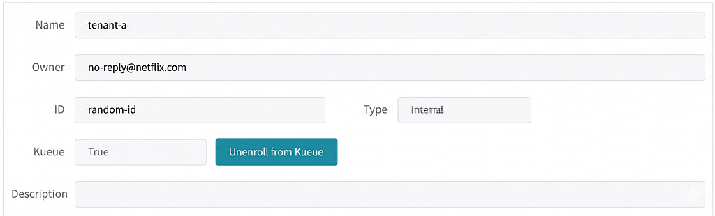
Leveraging Kubernetes virtual machines at Cloudflare with KubeVirt

Post Syndicated from Justin Cichra original https://blog.cloudflare.com/leveraging-kubernetes-virtual-machines-with-kubevirt

Cloudflare runs several multi-tenant Kubernetes clusters across our core data centers. These general-purpose clusters run on bare metal and power our control plane, analytics, and various engineering tools such as build infrastructure and continuous integration.

Kubernetes is a container orchestration platform. It enables software engineers to deploy containerized applications to a cluster of machines. This enables teams to build highly-available software on a scalable and resilient platform.

In this blog post we discuss our Kubernetes architecture, why we needed virtualization, and how we’re using it today.

Multi-tenant clusters

Multi-tenancy is a concept where one system can share its resources among a wide range of customers. This model allows us to build and manage a small number of general purpose Kubernetes clusters for our internal application teams. Keeping the number of clusters small reduces our operational toil. This model shrinks costs and increases computational efficiency by sharing hardware. Multi-tenancy also allows us to scale more efficiently. Scaling is done at either a cluster or application level. Cluster operators scale the platform by adding more hardware. Teams scale their applications by updating their Kubernetes manifests. They can scale vertically by increasing their resource requests or horizontally by increasing the number of replicas.

All of our Kubernetes clusters are multi-tenant with various components enabled for a secure and resilient platform.

Pods are secured using the latest standards recommended by the Kubernetes project. We use Pod Security Admission (PSA) and Pod Security Standards to ensure all workloads are following best practices. By default, all namespaces use the most restrictive profile, and only a few Kubernetes control plane namespaces are granted privileged access. For additional policies not covered by PSA, we built custom Validating Webhooks on top of the controller-runtime framework. PSA and our custom policies ensure clusters are secure and workloads are isolated.

Our need for virtualization

A select number of teams needed tight integration with the Linux kernel. Examples include Docker daemons for build infrastructure and the ability to simulate servers running the software and configuration of our global network. With our pod security requirements, these workloads are not permitted to interface with the host kernel at a deep level (e.g. no iptables or sysctls). Doing so may disrupt other tenants sharing the node and open additional attack vectors if an application was compromised. A virtualization platform would enable these workloads to interact with their own kernel within a secured Kubernetes cluster.

We considered various different virtualization solutions. Running a separate virtualization platform outside of Kubernetes would have worked, but would not tightly integrate containerized workloads with virtual machines. It would also be an additional operational burden on our team, as backups, alerting, and fleet management would have to exist for both our Kubernetes and virtual machine clusters.

We then looked for solutions that run virtual machines within Kubernetes. Teams could already manually deploy QEMU pods, but this was not an elegant solution. We needed a better way. There were several other options, but KubeVirt was the tool that met the majority of our requirements. Other solutions required a privileged container to run a virtual machine, but KubeVirt did not – this was a crucial requirement in our goal of creating a more secure multi-tenant cluster. KubeVirt also uses a feature of the Kubernetes API called Custom Resource Definitions (CRDs), which extends the Kubernetes API with new objects, increasing the flexibility of Kubernetes beyond its built-in types. For KubeVirt, this includes objects such as VirtualMachine and VirtualMachineInstanceReplicaSet. We felt the use of CRDs would allow KubeVirt to grow as more features were added.

What is KubeVirt?

KubeVirt is a virtualization platform that enables users to run virtual machines within Kubernetes. With KubeVirt, virtual machines run alongside containerized workloads on the same platform. Kubernetes primitives such as network policies, configmaps, and services all integrate with virtual machines. KubeVirt scales with our needs and is successfully running hundreds of virtual machines across several clusters. We frequently remediate Kubernetes nodes, so virtual machines and pods are always exercising their startup/shutdown processes.

How Cloudflare uses KubeVirt

There are a number of internal projects leveraging virtual machines at Cloudflare. We’ll touch on a few of our more popular use cases:

  1. Kubernetes scalability testing

  2. Development environments

  3. Kernel and iPXE testing

  4. Build pipelines

Kubernetes scalability testing

Setup process

Our staging clusters are much smaller than our largest production clusters. They also run on bare metal and mirror the configuration we have for each production cluster. This is extremely useful when rolling out new software, operating systems, or kernel changes; however, they miss bugs that only surface at scale. We use KubeVirt to bridge this gap and virtualize Kubernetes clusters with hundreds of nodes and thousands of pods.

The setup process for virtualized clusters differs from our bare metal provisioning steps. For bare metal, we use Salt to provision clusters from start to finish. For our virtualized clusters we use Ansible and kubeadm.  Our bare metal staging clusters are responsible for testing and validating our Salt configuration. The virtualized clusters give us a vanilla Kubernetes environment without any Cloudflare customizations. Having a stock environment in addition to our Salt environment helps us isolate bugs down to a Kubernetes change, a kernel change, or a Cloudflare-specific configuration change.

Our virtualized clusters consist of a KubeVirt VirtualMachine object per node. We create three control-plane nodes and any number of worker nodes. Each virtual machine starts out as a vanilla Debian generic cloud image. Using KubeVirt’s cloud-init support, the virtual machine downloads an internal Ansible playbook which installs a recent kernel, cri-o (the container runtime we use), and kubeadm.

- name: Add the Kubernetes gpg key
  apt_key:
    url: https://pkgs.k8s.io/core:/stable:/{{ kube_version }}/deb/Release.key
    keyring: /etc/apt/keyrings/kubernetes-apt-keyring.gpg
    state: present

- name: Add the Kubernetes repository
  shell: echo "deb [signed-by=/etc/apt/keyrings/kubernetes-apt-keyring.gpg] https://pkgs.k8s.io/core:/stable:/{{ kube_version }}/deb/ /" | tee /etc/apt/sources.list.d/kubernetes.list

- name: Add the CRI-O gpg key
  apt_key:
    url: https://pkgs.k8s.io/addons:/cri-o:/{{ crio_version }}/deb/Release.key
    keyring: /etc/apt/keyrings/cri-o-apt-keyring.gpg
    state: present

- name: Add the CRI-O repository
  shell: echo "deb [signed-by=/etc/apt/keyrings/cri-o-apt-keyring.gpg] https://pkgs.k8s.io/addons:/cri-o:/{{ crio_version }}/deb/ /" | tee /etc/apt/sources.list.d/cri-o.list

- name: Install CRI-O and Kubernetes packages
  apt:
    name:
      - cri-o
      - kubelet
      - kubeadm
      - kubectl
    update_cache: yes
    state: present

- name: Enable and start CRI-O service
  service:
    state: started
    enabled: yes
    name: crio.service

Ansible playbook steps to download and install Kubernetes tooling

Once each node has completed its individual playbook, we can initialize and join nodes to the cluster using another playbook that runs kubeadm. From there the cluster can be accessed by logging into a control plane node using kubectl.

Simulating at scale

When losing 10s or 100s of nodes at once, Kubernetes needs to act quickly to minimize downtime. The sooner it recognizes node failure, the faster it can reroute traffic to healthy pods.

Using Kubernetes in KubeVirt we are able to simulate a large cluster undergoing a network cut and observe how Kubernetes reacts. The KubeVirt Kubernetes cluster allows us to rapidly iterate on configuration changes and code patches.

The following Ansible playbook task simulates a network segmentation failure where only the control-plane nodes remain online.

- name: Disable network interfaces on all workers
  command: ifconfig enp1s0 down
  async: 5
  poll: 0
  ignore_errors: yes
  when: inventory_hostname in groups['kube-node']

An Ansible role which disables the network on all worker nodes simultaneously.

This framework allows us to exercise the code in controller-manager, Kubernetes’s daemon that reconciles the fundamental state of the system (Nodes, Pods, etc). Our simulation platform helped us drastically shorten full traffic recovery time when a large number of Kubernetes nodes become unreachable. We upstreamed our changes to Kubernetes and more controller-manager speed improvements are coming soon.

Development environments

Compiling code on your laptop can be slow. Perhaps you’re working on a patch for a large open-source project (e.g. V8 or Clickhouse) or need more bandwidth to upload and download containers. With KubeVirt, we enable our developers to rapidly iterate on software development and testing on powerful server hardware. KubeVirt integrates with Kubernetes Persistent Volumes, which enables teams to persist their development environment across restarts.

There are a number of teams at Cloudflare using KubeVirt for a variety of development and testing environments. Most notably is a project called Edge Test Fleet, which emulates a physical server and all the software that runs Cloudflare’s global network. Teams can test their code and configuration changes against the entire software stack without reserving dedicated hardware. Cloudflare uses Salt to provision systems. It can be difficult to iterate and test Salt changes without a complete virtual environment. Edge Test Fleet makes iterating on Salt easier, ensuring states compile and render the right output. With Edge Test Fleet, new developers can better understand how Cloudflare’s global network works without touching staging or production.

Additionally, one Cloudflare team developed a framework that allows users to build and test changes to Clickhouse using a VSCode environment. This framework is generally applicable to all teams requiring a development environment. Once a template environment is provisioned, CSI Volume Cloning can duplicate a golden volume, separating persistent environments for each developer.

apiVersion: v1
kind: PersistentVolumeClaim
name: devspace-jcichra-rootfs
namespace: dev-clickhouse-vms
spec:
  accessModes:
  - ReadWriteOnce
  storageClassName: rook-ceph-nvme
  dataSource:
    kind: PersistentVolumeClaim
    name: dev-rootfs
  resources:
    requests:
      storage: 500Gi

A PersistentVolumeClaim that clones data from another volume using CSI Volume Cloning

Kernel and iPXE testing

Unlike user space software development, when a kernel crashes, the entire system crashes. The kernel team uses KubeVirt for development. KubeVirt gives all kernel engineers, regardless of laptop OS or architecture, the same x86 environment and hypervisor. Virtual machines on server hardware can be scaled up to more cores and memory than on laptops. The Cloudflare kernel team has also found low-level issues which only surface in environments with many CPUs.

To make testing fast and easy, the kernel team serves iPXE images via an nginx Pod and Service adjacent to the virtual machine. A recent kernel and Debian image are copied to the nginx pod via kubectl cp. The iPXE file can then be referenced in the KubeVirt virtual machine definition via the DNS name for the Kubernetes Service.

interfaces:
  name: default
  masquerade: {}
  model: e1000e
  ports:
    - port: 22
      dhcpOptions:
        bootFileName: http://httpboot.u-$K8S_USER.svc.cluster.local/boot.ipxe

When the virtual machine boots, it will get an IP address on the default interface behind NAT due to our masquerade setting. Then it will download boot.ipxe, which describes what additional files should be downloaded to start the system. In this case, the kernel (vmlinuz-amd64), Debian (baseimg-amd64.img) and additional kernel modules (modules-amd64.img) are downloaded.


UEFI iPXE boot connecting and downloading files from nginx pod in user’s namespace

Once the system is booted, a developer can log in to the system for testing:

linux login: root
Password: 
Linux linux 6.6.35-cloudflare-2024.6.7 #1 SMP PREEMPT_DYNAMIC Mon Sep 27 00:00:00 UTC 2010 x86_64

The programs included with the Debian GNU/Linux system are free software;
the exact distribution terms for each program are described in the
individual files in /usr/share/doc/*/copyright.

Debian GNU/Linux comes with ABSOLUTELY NO WARRANTY, to the extent
permitted by applicable law.
root@linux:~# 

Custom kernels can be copied to the nginx pod via kubectl cp. Restarting the virtual machine will load that new kernel for testing. When a kernel panic occurs, the virtual machine can quickly be restarted with virtctl restart linux and it will go through the iPXE boot process again.

Build pipelines

Cloudflare leverages KubeVirt to build a majority of software at Cloudflare. Virtual machines give build system users full control over their pipeline. For example, Debian packages can easily be installed and separate container daemons (such as Docker) can run all within a Kubernetes namespace using the restricted Pod Security Standard. KubeVirt’s VirtualMachineReplicaSet concept allows us to quickly scale up and down the number of build agents to match demand. We can roll out different sets of virtual machines with varying sizes, kernels, and operating systems.

To scale efficiently, we leverage container disks to store our agent virtual machine images. Container disks allow us to store the virtual machine image (for example, a qcow image) in our container registry. This strategy works well when the state in virtual machines is ephemeral. Liveness probes detect unhealthy or broken agents, shutting down the virtual machine and replacing them with a fresh instance. Other automation limits virtual machine uptime, capping it to 3–4 hours to keep build agents fresh.

Next steps

We’re excited to expand our use of KubeVirt and unlock new capabilities for our internal users. KubeVirt’s Linux ARM64 support will allow us to build ARM64 packages in-cluster and simulate ARM64 systems.

Projects like KubeVirt CDI (Containerized Data Importer) will streamline our user’s virtual machine experience. Instead of users manually building container disks, we can provide a catalog of virtual machine images. It also allows us to copy virtual machine disks between namespaces.

Conclusion

KubeVirt has proven to be a great tool for virtualization in our Kubernetes-first environment. We’ve unlocked the ability to support more workloads with our multi-tenant model. The KubeVirt platform allows us to offer a single compute platform supporting containers and virtual machines. Managing it has been simple, and upgrades have been straightforward and non-disruptive. We’re exploring additional features KubeVirt offers to improve the experience for our users.

Finally, our team is expanding! We’re looking for more people passionate about Kubernetes to join our team and help us push Kubernetes to the next level.

Evolution of Catwalk: Model serving platform at Grab

Post Syndicated from Grab Tech original https://engineering.grab.com/catwalk-evolution

Introduction

As Southeast Asia’s leading super app, Grab serves millions of users across multiple countries every day. Our services range from ride-hailing and food delivery to digital payments and much more. The backbone of our operations? Machine Learning (ML) models. They power our real-time decision-making capabilities, enabling us to provide a seamless and personalised experience to our users. Whether it’s determining the most efficient route for a ride, suggesting a food outlet based on a user’s preference, or detecting fraudulent transactions, ML models are at the forefront.

However, serving these ML models at Grab’s scale is no small feat. It requires a robust, efficient, and scalable model serving platform, which is where our ML model serving platform, Catwalk, comes in.

Catwalk has evolved over time, adapting to the growing needs of our business and the ever-changing tech landscape. It has been a journey of continuous learning and improvement, with each step bringing new challenges and opportunities.

Evolution of the platform

Phase 0: The need for a model serving platform

Before Catwalk’s debut as our dedicated model serving platform, data scientists across the company employed various ad-hoc approaches to serve ML models. These included:

  • Shipping models online using custom solutions.
  • Relying on backend engineering teams to deploy and manage trained ML models.
  • Embedding ML logic within Go backend services.

These methods, however, led to several challenges, undercovering the need for a unified, company-wide platform for serving machine learning models:

  • Operational overhead: Data scientists often lacked the necessary expertise to handle the operational aspects of their models, leading to service outages.
  • Resource wastage: There was frequently low resource utilisation (e.g., 1%) for data science services, leading to inefficient use of resources.
  • Friction with engineering teams: Differences in release cycles and unclear ownership when code was embedded into backend systems resulted in tension between data scientists and engineers.
  • Reinventing the wheel: Multiple teams independently attempted to solve model serving problems, leading to a duplication of effort.

​​These challenges highlighted the need for a company-wide, centralised platform for serving machine learning models.

Phase 1: No-code, managed platform for TensorFlow Serving models

Our initial foray into model serving was centred around creating a managed platform for deploying TensorFlow Serving models. The process involved data scientists submitting their models to the platform’s engineering admin, who could then deploy the model with an endpoint. Infrastructure and networking were managed using Amazon Elastic Kubernetes Service (EKS) and Helm Charts as illustrated below.


This phase of our platform, which we also detailed in our previous article, was beneficial for some users. However, we quickly encountered scalability challenges:

  • Codebase maintenance: Applying changes to every TensorFlow Serving (TFS) version was cumbersome and difficult to maintain.
  • Limited scalability: The fully managed nature of the platform made it difficult to scale.
  • Admin bottleneck: The engineering admin’s limited bandwidth became a bottleneck for onboarding new models.
  • Limited serving types: The platform only supported TensorFlow, limiting its usefulness for data scientists using other frameworks like LightGBM, XGBoost, or PyTorch.

After a year of operation, only eight models were onboarded to the platform, highlighting the need for a more scalable and flexible solution.

Phase 2: From models to model serving applications

To address the limitations of Phase 1, we transitioned from deploying individual models to self-contained model serving applications. This “low-code, self-serving” strategy introduced several new components and changes as illustrated in the points and diagram below:

  • Support for multiple serving types: Users gained the ability to deploy models trained with a variety of frameworks like Open Neural Network Exchange (ONNX), PyTorch, and TensorFlow.
  • Self-served platform through CI/CD pipelines: Data scientists could self-serve and independently manage their model serving applications through CI/CD pipelines.
  • New components: We introduced these new components to support the self-serving approach:
    • Catwalk proxy, a managed reverse proxy to various serving types.
    • Catwalk transformer, a low-code component to transform input and output data.
    • Amphawa, a feature fetching component to augment model inputs.

API request flow

The Catwalk proxy acts as the orchestration layer. Clients send requests to Catwalk proxy then it orchestrates calls to different components like transformers, feature-store, and so on. A typical end to end request flow is illustrated below.


Within a year of implementing these changes, the number of models on the platform increased from 8 to 300, demonstrating the success of this approach. However, new challenges emerged:

  • Complexity of maintaining Helm chart: As the platform continued to grow with new components and functionalities, maintaining the Helm chart became increasingly complex. The readability and flow control became more challenging, making the helm chart updating process prone to errors.
  • Process-level mistakes: The self-serving approach led to errors such as pushing empty or incompatible models to production, setting too few replicas, or allocating insufficient resources, which resulted in service crashes.

We knew that our work was nowhere near done. We had to keep iterating and explore ways to address the new challenges.

Phase 3: Replacing Helm charts with Kubernetes CRDs

To tackle the deployment challenges and gain more control, we made the significant decision to replace Helm charts with Kubernetes Custom Resource Definitions (CRDs). This required substantial engineering effort, but the outcomes have been rewarding. This transition gave us improved control over deployment pipelines, enabling customisations such as:

  • Smart defaults for AutoML
  • Blue-green deployments
  • Capacity management
  • Advanced scaling
  • Application set groupings

Below is an example of a simple model serving CRD manifest:

apiVersion: ml.catwalk.kubebuilder.io/v1
kind: ModelServing
spec:
  hpa:
    desired: 1
    max: 1
    min: 1
  modelMeta:
    modelName: "my-model"
    modelOwner: john.doe
  proxyLayer:
    enableLogging: true
    logHTTPBody: true
  servingLayer:
    servingType: "tensorflow-serving"
    version: "20"

Model serving CRD deployment state machine

Every model serving CRD submission follows a sequence of steps. If there are failures at any step, the controller keeps retrying after small intervals. The major steps on the deployment cycle are described below:

  1. Validate whether the new CRD specs are acceptable. Along with sanity checks, we also enforce a lot of platform constraints through this step.
  2. Clean up previous non-ready deployment resources. Sometimes a deployment submission might keep crashing and hence it doesn’t proceed to a ready state. On every submission, it’s important to check and clean up such previous deployments.
  3. Create resources for the new deployment and ensure that the new deployment is ready.
  4. Switch traffic from old deployment to the new deployment.
  5. Clean up resources for old deployment. At this point, traffic is already being served by the new deployment resources. So, we can clean up the old deployment.

Phase 4: Transition to a high-code, self-served, process-managed platform

As the number of model serving applications and use cases multiplied, clients sought greater control over orchestrations between different models, experiment executions, traffic shadowing, and responses archiving. To cater to these needs, we introduced several changes and components with the Catwalk Orchestrator, a high code orchestration solution, leading the pack.

Catwalk orchestrator

The Catwalk Orchestrator is a highly abstracted framework for building ML applications that replaced the catwalk-proxy from previous phases. The key difference is that users can now write their own business/orchestration logic. The orchestrator offers a range of utilities, reducing the need for users to write extensive boilerplate code. Key components of the Catwalk Orchestrator include HTTP server, gRPC server, clients for different model serving flavours (TensorFlow, ONNX, PyTorch, etc), client for fetching features from the feature bank, and utilities for logging, metrics, and data lake ingestion.

The Catwalk Orchestrator is designed to streamline the deployment of machine learning models. Here’s a typical user journey:

  1. Scaffold a model serving application: Users begin by scaffolding a model serving application using a command-line tool.
  2. Write business logic: Users then write the business logic for the application.
  3. Deploy to staging: The application is then deployed to a staging environment for testing.
  4. Complete load testing: Users test the application in the staging environment and complete load testing to ensure it can handle the expected traffic.
  5. Deploy to production: Once testing is completed, the application is deployed to the production environment.

Bundled deployments

To support multiple ML models as part of a single model serving application, we introduced the concept of bundled deployments. Multiple Kubernetes deployments are bundled together as a single model serving application deployment, allowing each component (e.g., models, catwalk-orchestrator, etc) to have its own Kubernetes deployment and to scale independently.


In addition to the major developments, we implemented other changes to enhance our platform’s efficiency. We made load testing mandatory for all ML application updates to ensure robust performance. This testing process was streamlined with a single command that runs the load test in the staging environment, with the results directly shared with the user.

Furthermore, we boosted deployment transparency by sharing deployment details through Slack and Datadog. This empowered users to diagnose issues independently, reducing the dependency on on-call support. This transparency not only improved our issue resolution times but also enhanced user confidence in our platform.

The results of these changes speak for themselves. The Catwalk Orchestrator has evolved into our flagship product. In just two years, we have deployed 200 Catwalk Orchestrators serving approximately 1,400 ML models.

What’s next?

As we continue to innovate and enhance our model serving platform, we are venturing into new territories:

  • Catwalk serverless: We aim to further abstract the model serving experience, making it even more user-friendly and efficient.
  • Catwalk data serving: We are looking to extend Catwalk’s capabilities to serve data online, providing a more comprehensive service.
  • LLM serving: In line with the trend towards generative AI and large language models (LLMs), we’re pivoting Catwalk to support these developments, ensuring we stay at the forefront of the AI and machine learning field.

Stay tuned as we continue to advance our technology and bring these exciting developments to life.

Join us

Grab is the leading superapp platform in Southeast Asia, providing everyday services that matter to consumers. More than just a ride-hailing and food delivery app, Grab offers a wide range of on-demand services in the region, including mobility, food, package and grocery delivery services, mobile payments, and financial services across 700 cities in eight countries.

Powered by technology and driven by heart, our mission is to drive Southeast Asia forward by creating economic empowerment for everyone. If this mission speaks to you, join our team today!
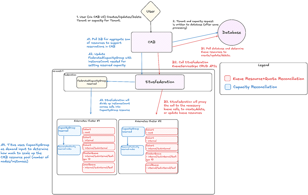
Simplify Amazon EKS Deployments with GitHub Actions and AWS CodeBuild

Post Syndicated from Deepak Kovvuri original https://aws.amazon.com/blogs/devops/simplify-amazon-eks-deployments-with-github-actions-and-aws-codebuild/

In this blog post, we will explore how to simplify Amazon EKS deployments with GitHub Actions and AWS CodeBuild. In today’s fast-paced digital landscape, organizations are turning to DevOps practices to drive innovation and streamline their software development and infrastructure management processes. One key practice within DevOps is Continuous Integration and Continuous Delivery (CI/CD), which automates deployment activities to reduce the time it takes to release new software updates. AWS offers a suite of native tools to support CI/CD, but also allows for flexibility and customization through integration with third-party tools.

Throughout this post, you will learn how to use GitHub Actions to create a CI/CD workflow with AWS CodeBuild and AWS CodePipeline. You’ll leverage the capabilities of GitHub Actions from a vast selection of pre-written actions in the GitHub Marketplace to build and deploy a Python application to an Amazon Elastic Kubernetes Service (EKS) cluster.

GitHub Actions is a powerful feature on GitHub’s development platform that enables you to automate your software development workflows directly within your repository. With Actions, you can write individual tasks to build, test, package, release, or deploy your code, and then combine them into custom workflows to streamline your development process.

Solution Overview

This solution being proposed in this post uses several AWS developer tools to establish a CI/CD pipeline while ensuring a streamlined path from development to deployment:

  • AWS CodeBuild: A fully managed build service that compiles source code, runs tests, and produces software packages that are ready to deploy.
  • AWS CodePipeline: A continuous delivery service that orchestrates the build, test, and deploy phases of your release process.
  • Amazon Elastic Kubernetes Service (EKS): A managed service that makes it easy to run Kubernetes on AWS without needing to install and operate your own Kubernetes control plane.
  • AWS CloudFormation: AWS CloudFormation lets you model, provision, and manage AWS and third-party resources by treating infrastructure as code. You’ll use AWS CloudFormation to deploy certain baseline resources required to follow along.
  • Amazon Elastic Container Registry (ECR): A fully managed container registry that makes it easy for developers to store, manage, and deploy Docker container images.
Figure 1 Workflow architecture showing source, build, test, approval and deployment stages

Figure 1 Workflow architecture showing source, build, test, approval and deployment stages

The code’s journey from the developer’s workstation to the final user-facing application is a seamless relay across various AWS services with key build an deploy operations performed via GitHub Actions:

  1. The developer commits the application’s code to the Source Code Repository. In this post we will leverage a repository created in AWS CodeCommit.
  2. The commit to the Source Control Management (SCM) system triggers the AWS CodePipeline, which is the orchestration service that manages the CI/CD pipeline.
  3. AWS CodePipeline proceeds to the Build stage, where AWS CodeBuild, integrated with GitHub Actions, builds the container image from the committed code.
  4. Once the container image is successfully built, AWS CodeBuild, with GitHub Actions, pushes the image to Amazon Elastic Container Registry (ECR) for storage and versioning.
  5. An Approval Stage is included in the pipeline, which allows the developer to manually review and approve the build artifacts before they are deployed.
  6. After receiving approval, AWS CodePipeline advances to the Deploy Stage, where GitHub Actions are used to run helm deployment commands.
  7. Within this Deploy Stage, AWS CodeBuild uses GitHub Actions to install the Helm application on Amazon Elastic Kubernetes Service (EKS), leveraging Helm charts for deployment.
  8. The deployed application is now running on Amazon EKS and is accessible via the automatically provisioned Application Load Balancer.

Pre-requisites

If you choose to replicate the steps in this post, you will need the following items:

Utilities like awscli and eksctl require access to your AWS account. Please make sure you have the AWS CLI configured with credentials. For instructions on setting up the AWS CLI, refer to this documentation.

Walkthrough

Deploy Baseline Resources

To get started you will first deploy an AWS CloudFormation stack that pre-creates some foundational developer resources such as a CodeCommit repository, CodeBuild projects, a CodePipeline pipeline that orchestrates the release of the application across multiple stages. If you’re interested to learn more about the resources being deployed, you can download the template and review its contents.

Additionally, to make use of GitHub Actions in AWS CodeBuild, it is required to authenticate your AWS CodeBuild project with GitHub using an access token – authentication with GitHub is required to ensure consistent access and avoid being rate-limited by GitHub.

  1. First, let’s set up the environment variables required to configure the infrastructure:
    export CLUSTER_NAME=<cluster-name>
    export AWS_REGION=<cluster-region>
    export AWS_ACCOUNT_ID=<cluster-account>
    export GITHUB_TOKEN=<github-pat>

    In the commands above, replace cluster-name with your EKS cluster name, cluster-region with the AWS region of your EKS cluster, cluster-account with your AWS account ID (12-digit number), and github-pat with your GitHub Personal Access Token (PAT).

  2. Using the AWS CloudFormation template located here, deploy the stack using the AWS CLI:
    aws cloudformation create-stack \
      --stack-name github-actions-demo-base \
      --region $AWS_REGION \
      --template-body file://gha.yaml \
      --parameters ParameterKey=ClusterName,ParameterValue=$CLUSTER_NAME \
                   ParameterKey=RepositoryToken,ParameterValue=$GITHUB_TOKEN \
      --capabilities CAPABILITY_IAM && \
    echo "Waiting for stack to be created..." && \
    aws cloudformation wait stack-create-complete \
      --stack-name github-actions-demo-base \
      --region $AWS_REGION
  3. When you use AWS CodeBuild / GitHub Actions to deploy your application onto Amazon EKS, you’ll need to allow-list the service role associated with the build project(s) by adding the IAM principal to access your Cluster’s aws-auth config-map or using EKS Access Entries (recommended). The CodeBuild service role has been pre-created in the previous step and the role ARN can be retrieved using the command below:
    aws cloudformation describe-stacks --stack-name github-actions-demo-base \
    --query "Stacks[0].Outputs[?OutputKey=='CodeBuildServiceRole'].OutputValue" \
    --region $AWS_REGION --output text

Clone the CodeCommit Repository

Next, you will create a simple python flask application and the associated helm charts required to deploy the application and commit them to source control repository in AWS CodeCommit. Begin by cloning the CodeCommit repository by following the steps below:

  1. Configure your git client to use the AWS CLI CodeCommit credential helper. For UNIX based systems follow instructions here, and for Windows based systems follow instructions here.
  2. Retrieve the repository HTTPS clone URL using the command below:
    export CODECOMMIT_CLONE_URL=$(aws cloudformation describe-stacks \
    --stack-name github-actions-demo-base \
    --query "Stacks[0].Outputs[?OutputKey=='CodeCommitCloneUrl'].OutputValue" \
    --region $AWS_REGION \
    --output text)
  3. Clone and navigate to your repository:
    git clone $CODECOMMIT_CLONE_URL github-actions-demo && cd github-actions-demo

Create the Application

Now that you’ve set up all the required resources, you can begin building your application and its necessary deployment manifests.

  1. Create the app.py file, which serves as the hello world application using the command below:
    cat << EOF >app.py
    from flask import Flask
    app = Flask(__name__)
    
    @app.route('/')
    def demoapp():
      return 'Hello from EKS! This application is built using Github Actions on AWS CodeBuild'
    
    if __name__ == '__main__':
      app.run(port=8080,host='0.0.0.0')
    EOF
  2. Create a Dockerfile in the same directory as the application using the command below:
    cat << EOF > Dockerfile
    FROM public.ecr.aws/docker/library/python:alpine3.18 
    WORKDIR /app 
    RUN pip install Flask 
    RUN apk update && apk upgrade --no-cache 
    COPY app.py . 
    CMD [ "python3", "app.py" ]
    EOF
  3. Initialize the HELM application
    helm create demo-app
    rm -rf demo-app/templates/*
  4. Create the manifest files required for the deployment accordingly:
    • deployment.yaml – Contains the blueprint for deploying instances of the application. It includes the desired state and pod template which has the pod specifications like the container image to be used, ports etc.
      cat <<EOF > demo-app/templates/deployment.yaml
      ---
      apiVersion: apps/v1
      kind: Deployment
      metadata:
        namespace: {{ default "default" .Values.namespace }}
        name: {{ .Release.Name }}-deployment
      spec:
        selector:
          matchLabels:
            app.kubernetes.io/name: {{ .Release.Name }}
        replicas: 2
        template:
          metadata:
            labels:
              app.kubernetes.io/name: {{ .Release.Name }}
          spec:
            containers:
            - image: {{ .Values.image.repository }}:{{ default "latest" .Values.image.tag }}
              imagePullPolicy: {{ .Values.image.pullPolicy}}
              name: demoapp
              ports:
              - containerPort: 8080
      EOF
    • service.yaml – Describes the service object in Kubernetes and specifies how to access the set of pods running the application. It acts as an internal load balancer to route traffic to pods based on the defined service type (like ClusterIP, NodePort, or LoadBalancer).
      cat <<EOF > demo-app/templates/service.yaml
      ---
      apiVersion: v1
      kind: Service
      metadata:
        namespace: {{ default "default" .Values.namespace }}
        name: {{ .Release.Name }}-service
      spec:
        ports:
          - port: {{ .Values.service.port }}
            targetPort: 8080
            protocol: TCP
        type: {{ .Values.service.type }}
        selector:
          app.kubernetes.io/name: {{ .Release.Name }}
      EOF
    • ingress.yaml – Defines the ingress rules for accessing the application from outside the Kubernetes cluster. This file maps HTTP and HTTPS routes to services within the cluster, allowing external traffic to reach the correct services.
      cat <<EOF > demo-app/templates/ingress.yaml
      ---
      apiVersion: networking.k8s.io/v1
      kind: Ingress
      metadata:
        namespace: {{ default "default" .Values.namespace }}
        name: {{ .Release.Name }}-ingress
        annotations:
          alb.ingress.kubernetes.io/scheme: internet-facing
          alb.ingress.kubernetes.io/target-type: ip
      spec:
        ingressClassName: alb
        rules:
          - http:
              paths:
              - path: /
                pathType: Prefix
                backend:
                  service:
                    name: {{ .Release.Name }}-service
                    port:
                      number: 8080
      EOF
    • values.yaml – This file provides the default configuration values for the Helm chart. This file is crucial for customizing the chart to fit different environments or deployment scenarios. The manifest below assumes that the default namespace is configured as the namespace selector for your Fargate profile.
      cat <<EOF > demo-app/values.yaml
      ---
      namespace: default
      replicaCount: 1
      image:
        pullPolicy: IfNotPresent
      service:
        type: NodePort
        port: 8080
      EOF

Overview of the CI/CD Pipeline

  • A typical CI/CD pipeline consists of source, build, test, approval, and deploy stages.
  • In this post, AWS CodeBuild is used in the build and deploy states. AWS CodeBuild utilizes specification files called buildspec.
  • A buildspec is a collection of build phases and relevant settings in YAML format that CodeBuild uses to execute a build.

Below you’ll learn how to define your buildspec(s) to build and deploy your application onto Amazon EKS by leveraging the AWS managed GitHub action runner on AWS CodeBuild.

Defining GitHub Actions in AWS CodeBuild

Each phase in a buildspec can contain multiple steps and each step can run commands or run a GitHub Action. Each step runs in its own process and has access to the build filesystem. A step references a GitHub action by specifying the uses directive and optionally the with directive is used to pass arguments required by the action. Alternatively, a step can specify a series of commands using the run directive. It’s worth noting that, because steps run in their own process, changes to environment variables are not preserved between steps.

To pass environment variables between different steps of a build phase, you will need to assign the value to an existing or new environment variable and then writing this to the GITHUB_ENV environment file. Additionally, these environment variables can also be passed across multiple stage in CodePipeline by leveraging the exported variables directive.

Build Specification (Build Stage)

Here, you will create a file called buildspec-build.yml at the root of the repository – In the following buildspec, we leverage GitHub actions in AWS CodeBuild to build the container image and push the image to ECR. The actions used in this buildspec are:

  • aws-actions/configure-aws-credentials: Accessing AWS APIs requires the action to be authenticated using AWS credentials. By default, the permissions granted to the CodeBuild service role can be used to sign API actions executed during a build. However, when using a GitHub action in CodeBuild, the credentials from the CodeBuild service role need to be made available to subsequent actions (e.g., to log in to ECR, push the image). This action allows leveraging the CodeBuild service role credentials for subsequent actions.
  • aws-actions/amazon-ecr-login: Logs into the ECR registry using the credentials from the previous step.
version: 0.2
env:
  exported-variables:
    - IMAGE_REPO
    - IMAGE_TAG
phases:
  build:
    steps:
      - name: Get CodeBuild Region
        run: |
          echo "AWS_REGION=$AWS_REGION" >> $GITHUB_ENV
      - name: "Configure AWS credentials"
        id: creds
        uses: aws-actions/configure-aws-credentials@v3
        with:
          aws-region: ${{ env.AWS_REGION }}
          output-credentials: true
      - name: "Login to Amazon ECR"
        id: login-ecr
        uses: aws-actions/amazon-ecr-login@v1
      - name: "Build, tag, and push the image to Amazon ECR"
        run: |
          IMAGE_TAG=$(echo $CODEBUILD_RESOLVED_SOURCE_VERSION | cut -c 1-7)
          docker build -t $IMAGE_REPO:latest .
          docker tag $IMAGE_REPO:latest $IMAGE_REPO:$IMAGE_TAG
          echo "$IMAGE_REPO:$IMAGE_TAG"
          echo "IMAGE_REPO=$IMAGE_REPO" >> $GITHUB_ENV
          echo "IMAGE_TAG=$IMAGE_TAG" >> $GITHUB_ENV
          echo "Pushing image to $REPOSITORY_URI"
          docker push $IMAGE_REPO:latest
          docker push $IMAGE_REPO:$IMAGE_TAG

In the buildspec above the variables IMAGE_REPO and IMAGE_TAG are set as exported-variables that will be used in the subsequent deploy stage.

Build Specification (Deploy Stage)

During the deploy stage, you will utilize AWS CodeBuild to deploy the helm manifests to EKS by leveraging the community provided bitovi/deploy-eks-helm action. Furthermore, the alexellis/arkade-get action is employed to install kubectl, which will be used later to describe the ingress controller and retrieve the application URL.

Create a file called buildspec-deploy.yml at the root of the repository as such:

version: 0.2
env:
  exported-variables:
   - APP_URL
phases:
  build:
    steps:
      - name: "Get Build Region"
        run: |
          echo "AWS_REGION=$AWS_REGION" >> $GITHUB_ENV        
      - name: "Configure AWS credentials"
        uses: aws-actions/configure-aws-credentials@v3
        with:
          aws-region: ${{ env.AWS_REGION }}
      - name: "Install Kubectl"
        uses: alexellis/arkade-get@23907b6f8cec5667c9a4ef724adea073d677e221
        with:
          kubectl: latest
      - name: "Configure Kubectl"
        run: aws eks update-kubeconfig --name $CLUSTER_NAME
      - name: Deploy Helm
        uses: bitovi/[email protected]
        with:
          aws-region: ${{ env.AWS_REGION }}
          cluster-name: ${{ env.CLUSTER_NAME }}
          config-files: demo-app/values.yaml
          chart-path: demo-app/
          values: image.repository=${{ env.IMAGE_REPO }},image.tag=${{ env.IMAGE_TAG }}
          namespace: default
          name: demo-app
      - name: "Fetch Application URL"
        run: |
          while :;do url=$(kubectl get ingress/demo-app-ingress -o jsonpath='{.status.loadBalancer.ingress[0].hostname}' -n default);[ -z "$url" ]&&{ echo "URL is empty, retrying in 5 seconds...";sleep 5;}||{ export APP_URL="$url";echo "APP_URL set to: $APP_URL";break;};done;echo "APP_URL=$APP_URL">>$GITHUB_ENV 

At this point your application structure should have the following structure:

├── Dockerfile
├── app.py
├── buildspec-build.yml
├── buildspec-deploy.yml
└── demo-app
├── Chart.yaml
├── charts
├── templates
│ ├── deployment.yaml
│ ├── ingress.yaml
│ └── service.yaml
└── values.yaml

Now check these files in to the remote repository by running the below commands

git add -A && git commit -m "Initial Commit"
git push --set-upstream origin main

Now, let’s verify the deployment of our application using the load balancer URL. Navigate to the CodePipeline console. The pipeline incorporates a manual approval stage and requires a pipeline operator to review and approve the release to deploy the application. Following this, the URL for the deployed application can be conveniently retrieved from the outputs of the pipeline execution.

Viewing the application

    1. Click the execution ID. This should take you to a detailed overview of the most recent execution.

      Figure 2 - CodePipeline Console showing the pipeline (release) execution ID.

      Figure 2 CodePipeline Console showing the pipeline (release) execution ID

    2. Under the Timeline tab, select the ‘Build’ action for the ‘Deploy’ stage.

      Figure 3 - Navigating to the timeline view and reviewing the details for the deploy stage

      Figure 3 Navigating to the timeline view and reviewing the details for the deploy stage

    3. Copy the application load balancer URL from the output variables.

      Figure 4 Copy the APP_URL from the Output Variables for the Deploy action

      Figure 4 Copy the APP_URL from the Output Variables for the Deploy action

    4. Paste the URL into a browser of your choice and you should see the message below.

      Figure 5 Preview of the application deployed on Amazon EKS

      Figure 5 Preview of the application deployed on Amazon EKS

You can also review the logs for your build and see the GitHub action at work from the AWS CodeBuild console.

Clean up

To avoid incurring future charges, you should clean up the resources that you created:

      • Delete the application by executing helm, this will remove the ALB that was provisioned
        helm uninstall demo-app
      • Delete the CloudFormation stack (github-actions-demo-base) by executing the below command
        aws cloudformation delete-stack \
                --stack-name github-actions-demo-base \
                -–region $AWS_REGION

Conclusion

In this walkthrough, you have learned how to leverage the powerful combination of GitHub Actions and AWS CodeBuild to simplify and automate the deployment of a Python application on Amazon EKS. This approach not only streamlines your deployment process but also ensures that your application is built and deployed securely. You can extend this pipeline by incorporating additional stages such as testing and security scanning, depending on your project’s needs. Additionally, this solution can be used for other programming languages.

Authors

Deepak Kovvuri

Deepak Kovvuri

Deepak Kovvuri is a Senior Solutions Architect at AWS supporting Enterprise Customers in the US East area. He has over 6 years of experience in helping customers architecting a DevOps strategy for their cloud workloads. Some of the areas Deepak focuses on are CI/CD, Systems Administration, Infrastructure as Code, Container Services. He holds a Masters in Computer Engineer from University of Illinois at Chicago.

Bharath Gajendran

Bharath Gajendran

Bharath Gajendran is a Technical Account Manager at AWS. He works with customers to build highly scalable, cost effective and fault tolerant workloads utilizing AWS. He is passionate about Containers, DevOps, Automation and open-source technologies.

Pawan Shrivastava

Pawan Shrivastava is a Partner Solution Architect at AWS in the WWPS team. He focusses on working with partners to provide technical guidance on AWS, collaborate with them to understand their technical requirements, and designing solutions to meet their specific needs. Pawan is passionate about DevOps, automation and CI CD pipelines. He enjoys watching MMA, playing cricket and working out in the gym.

Rethinking Stream Processing: Data Exploration

Post Syndicated from Grab Tech original https://engineering.grab.com/rethinking-streaming-processing-data-exploration

Introduction

In this digital age, companies collect multitudes of data that enable the tracking of business metrics and performance. Over the years, data analytics tools for data storage and processing have evolved from the days of Excel sheets and macros to more advanced Map Reduce model tools like Spark, Hadoop, and Hive. This evolution has allowed companies, including Grab, to perform modern analytics on the data ingested into the Data Lake, empowering them to make better data-driven business decisions. This form of data will be referenced within this document as “Offline Data”.

With innovations in stream processing technology like Spark and Flink, there is now more interest in unlocking value from streaming data. This form of continuously-generated data in high volume will be referenced within this document as “Online Data”. In the context of Grab, the streaming data is usually materialised as Kafka topics (“Kafka Stream”) as the result of stream processing in its framework. This data is largely unexplored until they are eventually sunk into the Data Lake as Offline Data, part of the data journey (see Figure 1 below). This induces some data latency before the data can be used by data analysts to inform decisions.

Figure 1. Simplified data journey for Offline Data vs. Online Data, from data generation to data analysis.

As seen in Figure 1 above, the Time to Value (“TTV”) of Online Data is shorter as compared to that of Offline Data in a simplified data journey from data generation to data analysis where complexities of data cleaning and transformation have been removed. This is because the role of the data analyst or data scientist (“Data End User”) has been enabled forward to the Kafka stage for Online Data instead of the Data Lake stage for Offline Data. We recognise that allowing earlier data exploration on Online Data allows Data End Users to build context around the data inputs they are using in an earlier stage. This can help them process Offline Data more meaningfully in subsequent stages. We are interested in opening up the possibility for Data End Users to at least explore the Online Data before they architect a full solution to clean and/or process the data directly or more efficiently post-ingestion into the Data Lake. After their data exploration, the users would have more information to decide whether to spin up a stream processing pipeline for Online Data, or to continue processing Offline Data with their current solution, but with a more refined understanding and logic strategy against their source data inputs. However, of course, in this blog, we acknowledge that not all analysis on Online Data could be done in this manner.

Problem statement

Online Data is underutilised within Grab mainly because of, among other reasons, difficulty in performing data exploration on data that is not yet properly stored in the Data Lake.

For the purpose of this blog post, we will focus only on the problem of exploration of Online Data because this problem is the precursor to allowing us to fully democratise such data.

The problem of data exploration manifests itself when Data End Users need to find the proper data inputs to base and develop their data models. These users would then often need to parse through a multitude of documentation and connect with multiple upstream data producers, to know the range of data signals that are currently available and understand what each data signal is trying to measure.

Given the ephemeral nature of Online Data, this implies that the lack of correct tool adoption to seamlessly perform quick tests with application logic on Online Data disincentivises the Data End Users to work on these Online Data. Testing such logic on Offline Data is generally much easier since iteration testing on the exact same dataset is possible.

This difficulty in performing data exploration including ad hoc queries on Online Data has therefore made development of stream processing applications hard for Data End Users, creating headwinds in Grab’s aim to evolve from making data-driven business decisions to also making data-driven operation decisions. Doing both would allow Grab to react much quicker to abrupt changes in its business landscape.

Adoption of Zeppelin notebook environment

To address the difficulty in performing data exploration on Online Data, we have adopted Apache Zeppelin, a web-based notebook that enables data-drive, interactive data analytics with the support of multiple interpreters to work with various data processing backends e.g. Spark, Flink. The full solution of the adopted Zeppelin notebook environment is enabled seamlessly within our internal data-streaming platform, through its control plane. If you are interested, you may check out our previous blog post titled An elegant platform for more details on the abovementioned streaming platform and its control plane.

Figure 2. Zeppelin login page via web-based notebook environment.

As seen from Figure 2 above, after successful creation of the Zeppelin cluster, users can log in with their generated credentials delivered to them via the integrated instant messenger, and start using the notebook environment.

Figure 3. Zeppelin programme flow in the notebook environment.

Figure 3 above explains the Zeppelin notebook programme flow as follows:

  • The users enter their queries into the notebook session and run querying statements interactively with the established web-based notebook session.
  • The queries are passed to the Flink interpreter within the cluster to generate the Flink job as a Jar file, to be then submitted to a Flink session cluster.
  • When the Flink session cluster job manager receives the job, it would spin up the corresponding Flink task managers (workers) to run the application and retrieve the results.
  • The query results would then be piped back to the notebook session, to be displayed back to the user on the notebook session.

Data query and visualisation

Figure 4. Example of simple select query of data on Kafka.
Note: All variable names, schema, values, and other details used in this article are only created for use as examples.

Flink has a planned roadmap to create a unified streaming language for both stream processing and data analytics. In line with the roadmap, we have based our Zeppelin solution on supporting Structured Query Language (“SQL”) as the query language of choice as seen in Figure 4 above. Data End Users can now write queries in SQL, which is a language that they are comfortable with, and perform adequate data exploration.

As discussed in this section, data exploration on streaming data at the Kafka stage by adopting the right tool enables Data End Users to seamlessly have visibility to quickly understand the current schema of a Kafka topic (explained more in the next section. This kind of data exploration also enables Data End Users to understand the type of data the Kafka topic represents, such as the ability to determine if a country code data field is in alpha-2 or alpha-3 format while the data is still part of streaming data. This might seem inconsequential and immediately identifiable even in Offline Data, but by enabling data exploration at an earlier stage in the data journey for Online Data, Data End Users have the opportunity to react much more quickly. For example, a change of expected country code format from the data producer would usually lead to errors in the downstream joins or other stream processing pipelines due to incompatible parsing or filtering of the modified country codes. Instead of waiting for the data to be ingested to Offline Data, users can investigate the issue with Online Data retrieved from Kafka.

Figure 5. Simple visualisation of queried data on Zeppelin’s notebook environment.
Note: All variable names, schema, values, and other details used in this article are only created for use as examples.

Besides query features, Zeppelin notebook provides simple visualisation and analytics of the off-the-shelf data as presented above in Figure 5. Furthermore, users are now able to perform interactive ad hoc queries on Online Data. These queries will eventually become much more advanced and/or effective SQL queries to be deployed as a streaming pipeline later on in the data journey. This reduces the inertia in setting up a separate development environment or learning other programming languages like Java or Scala during the development of streaming pipelines. With Zeppelin’s notebook environment, our Data End Users are more empowered to quickly derive value from Online Data.

Need for a more dynamic table schema derivation process

For the Data End Users performing data exploration on Online Data, we see a need for these users to derive the Data Definition Language (“DDL”) associated with a Kafka stream at an earlier stage of the data journey. Within Grab, even though Kafka streams are transmitted in Protobuf format and are thus structured, both the schema and the corresponding DDL changes are added over time as new fields. Typically, the data producer (service owners) and the data engineers responsible for the data ingestion pipeline coordinate to perform such updates. Since the Data End Users are not involved in such schema update processes nor do they directly interact with the data producers, many of them find the discovery of changes in the current Kafka stream schema an issue. Granted that this is an issue our metadata platform is actively solving using Datahub, we hope to also solve the challenge by being able to derive the DDL more dynamically within the tooling, for data exploration on Online Data to reduce friction.

Figure 6. Common functions to derive DDL of a Kafka Stream in SQL.
Note: All variable names, schema, values, and other details used in this article are only created for use as examples.

As seen from Figure 6 above, we have an integrated tooling for Data End Users to derive the DDL associated with a Kafka stream using SQL language. A Kafka stream in Grab’s context is a logical concept describing a Kafka topic, associating it with its metadata like Kafka bootstrap servers and associated Java class created by Protoc. This tool maps the Protobuf schema definition of a Kafka stream to a DDL, allowing it to be expressed and used in SQL language. This reduces the manual effort involved in creating these table definitions from scratch based on the associated Protobuf schema. Users can now derive the DDL associated with a Kafka stream more easily.

Mitigating risks arising from data exploration on Online Data – data access authorisation/audit

While we rethink stream processing and are open to options that enable data exploration on Online Data as mentioned above, we realised that new security requirements related to data access authorisation and maintaining proper audit trail have emerged. Even with Personally Identifiable Information (PII) obfuscation enforcement by our streaming pipeline, it means we need to implement stricter guardrails in place along with audit trails to ensure users only have access to what they are allowed to, and this access can be removed in a break-glass scenario. If you are interested, you may check out our previous blog post titled PII masking for privacy-grade machine learning for more details about how we enforce PII masking on machine learning data streaming pipelines.

To enable data access authorisation, we utilised Strimzi, the operator of running Kafka on Kubernetes. We integrated Strimzi’s Open Policy Agent (OPA) with Kafka to define policies that authorise specific read-only user access to specific Kafka Topics. The identification of users is done via mutualTLS (mTLS) connection with our Kafka clusters, where their user details are part of the SSL certificate details used for authentication.

With these tools in place, each user’s request to explore Online Data would be properly logged, and each data access can be controlled by an OPA policy managed by a central team.

If you are interested, you may check out our previous post Zero trust with Kafka where we discussed our efforts to continue strengthening the security of our data-streaming platform.

Impact

With the proliferation of our data-streaming platform, we expect to see improvements in the way our data becomes gradually democratised. We have already been receiving use cases from the Data End Users who are interested in validating a chain of events on Online Data, i.e. retrieving information of all events associated with a particular booking, which is not currently something that can be done easily.

More importantly, the tools in place for data exploration on Online Data form the foundation required for us to embark on our next step of the stream processing journey. This foundation makes the development and validation of the stream processing logic much quicker. This occurs when ad hoc queries in a notebook environment are possible, removing the need for local developer environment setups and the need to go through the whole pipeline deployment process for eventual validation of the developed logic. We believe that this would prove to reduce our lead time in creating stream processing pipelines significantly.

What’s next?

Our next step is to rethink further how our stream processing pipelines are defined and start to provision SQL as the unified streaming language of our pipelines. This helps facilitate better discussion between upstream data producers, data engineers, and Data End Users, since SQL is the common language among these stakeholders.

We will also explore handling schema discovery in a more controlled manner by utilising a Hive catalogue to store our Kafka table definitions. This removes the need for users to retrieve and run the table DDL statement for every session, making the data exploration experience even more seamless.

References

[1] Apache Zeppelin | Web-based notebook that enables data-driven, interactive data analytics and collaborative documents with SQL, Scala, Python, R and more.

[2] An elegant platform | Grab engineering blog.

[3] Apache Flink | Roadmap on Unified SQL Platform.

[4] ISO | ISO 3166 Country Codes.

[5] Protobuf (Protocol Buffers)| Language-neutral, platform-neutral extensible mechanisms for serializing structured data.

[6] Datahub | Extensible metadata platform that enables data discovery, data observability and federated governance to help tame the complexity of your data ecosystem.

[7] Protoc | Protocol buffer compiler installation.

[8] PII masking for privacy-grade machine learning | Grab engineering blog.

[9] Zero trust with Kafka | Grab engineering blog.

[10] Open Policy Agent (OPA) | Policy-based control for cloud native environments.

[11] Strimzi | Using Open Policy Agent with Strimzi and Apache Kafka.

[12] Confluent Documentation | Configure mTLS authentication and RBAC for kafka brokers.

Join us

Grab is the leading superapp platform in Southeast Asia, providing everyday services that matter to consumers. More than just a ride-hailing and food delivery app, Grab offers a wide range of on-demand services in the region, including mobility, food, package and grocery delivery services, mobile payments, and financial services across 428 cities in eight countries.

Powered by technology and driven by heart, our mission is to drive Southeast Asia forward by creating economic empowerment for everyone. If this mission speaks to you, join our team today!

Kafka on Kubernetes: Reloaded for fault tolerance

Post Syndicated from Grab Tech original https://engineering.grab.com/kafka-on-kubernetes

Introduction

Coban – Grab’s real-time data streaming platform – has been operating Kafka on Kubernetes with Strimzi in
production for about two years. In a previous article (Zero trust with Kafka), we explained how we leveraged Strimzi to enhance the security of our data streaming offering.

In this article, we are going to describe how we improved the fault tolerance of our initial design, to the point where we no longer need to intervene if a Kafka broker is unexpectedly terminated.

Problem statement

We operate Kafka in the AWS Cloud. For the Kafka on Kubernetes design described in this article, we rely on Amazon Elastic Kubernetes Service (EKS), the managed Kubernetes offering by AWS, with the worker nodes deployed as self-managed nodes on Amazon Elastic Compute Cloud (EC2).

To make our operations easier and limit the blast radius of any incidents, we deploy exactly one Kafka cluster for each EKS cluster. We also give a full worker node to each Kafka broker. In terms of storage, we initially relied on EC2 instances with non-volatile memory express (NVMe) instance store volumes for
maximal I/O performance. Also, each Kafka cluster is accessible beyond its own Virtual Private Cloud (VPC) via a VPC Endpoint Service.

Fig. 1 Initial design of a 3-node Kafka cluster running on Kubernetes.

Fig. 1 shows a logical view of our initial design of a 3-node Kafka on Kubernetes cluster, as typically run by Coban. The Zookeeper and Cruise-Control components are not shown for clarity.

There are four Kubernetes services (1): one for the initial connection – referred to as “bootstrap” – that redirects incoming traffic to any Kafka pods, plus one for each Kafka pod, for the clients to target each Kafka broker individually (a requirement to produce or consume from/to a partition that resides on any particular Kafka broker). Four different listeners on the Network Load Balancer (NLB) listening on four different TCP ports, enable the Kafka clients to target either the bootstrap
service or any particular Kafka broker they need to reach. This is very similar to what we previously described in Exposing a Kafka Cluster via a VPC Endpoint Service.

Each worker node hosts a single Kafka pod (2). The NVMe instance store volume is used to create a Kubernetes Persistent Volume (PV), attached to a pod via a Kubernetes Persistent Volume Claim (PVC).

Lastly, the worker nodes belong to Auto-Scaling Groups (ASG) (3), one by Availability Zone (AZ). Strimzi adds in node affinity to make sure that the brokers are evenly distributed across AZs. In this initial design, ASGs are not for auto-scaling though, because we want to keep the size of the cluster under control. We only use ASGs – with a fixed size – to facilitate manual scaling operation and to automatically replace the terminated worker nodes.

With this initial design, let us see what happens in case of such a worker node termination.

Fig. 2 Representation of a worker node termination. Node C is terminated and replaced by node D. However the Kafka broker 3 pod is unable to restart on node D.

Fig. 2 shows the worker node C being terminated along with its NVMe instance store volume C, and replaced (by the ASG) by a new worker node D and its new, empty NVMe instance store volume D. On start-up, the worker node D automatically joins the Kubernetes cluster. The Kafka broker 3 pod that was running on the faulty worker node C is scheduled to restart on the new worker node D.

Although the NVMe instance store volume C is terminated along with the worker node C, there is no data loss because all of our Kafka topics are configured with a minimum of three replicas. The data is poised to be copied over from the surviving Kafka brokers 1 and 2 back to Kafka broker 3, as soon as Kafka broker 3 is effectively restarted on the worker node D.

However, there are three fundamental issues with this initial design:

  1. The Kafka clients that were in the middle of producing or consuming to/from the partition leaders of Kafka broker 3 are suddenly facing connection errors, because the broker was not gracefully demoted beforehand.
  2. The target groups of the NLB for both the bootstrap connection and Kafka broker 3 still point to the worker node C. Therefore, the network communication from the NLB to Kafka broker 3 is broken. A manual reconfiguration of the target groups is required.
  3. The PVC associating the Kafka broker 3 pod with its instance store PV is unable to automatically switch to the new NVMe instance store volume of the worker node D. Indeed, static provisioning is an intrinsic characteristic of Kubernetes local volumes. The PVC is still in Bound state, so Kubernetes does not take any action. However, the actual storage beneath the PV does not exist anymore. Without any storage, the Kafka broker 3 pod is unable to start.

At this stage, the Kafka cluster is running in a degraded state with only two out of three brokers, until a Coban engineer intervenes to reconfigure the target groups of the NLB and delete the zombie PVC (this, in turn, triggers its re-creation by Strimzi, this time using the new instance store PV).

In the next section, we will see how we have managed to address the three issues mentioned above to make this design fault-tolerant.

Solution

Graceful Kafka shutdown

To minimise the disruption for the Kafka clients, we leveraged the AWS Node Termination Handler (NTH). This component provided by AWS for Kubernetes environments is able to cordon and drain a worker node that is going to be terminated. This draining, in turn, triggers a graceful shutdown of the Kafka
process by sending a polite SIGTERM signal to all pods running on the worker node that is being drained (instead of the brutal SIGKILL of a normal termination).

The termination events of interest that are captured by the NTH are:

  • Scale-in operations by an ASG.
  • Manual termination of an instance.
  • AWS maintenance events, typically EC2 instances scheduled for upcoming retirement.

This suffices for most of the disruptions our clusters can face in normal times and our common maintenance operations, such as terminating a worker node to refresh it. Only sudden hardware failures (AWS issue events) would fall through the cracks and still trigger errors on the Kafka client side.

The NTH comes in two modes: Instance Metadata Service (IMDS) and Queue Processor. We chose to go with the latter as it is able to capture a broader range of events, widening the fault tolerance capability.

Scale-in operations by an ASG

Fig. 3 Architecture of the NTH with the Queue Processor.

Fig. 3 shows the NTH with the Queue Processor in action, and how it reacts to a scale-in operation (typically triggered manually, during a maintenance operation):

  1. As soon as the scale-in operation is triggered, an Auto Scaling lifecycle hook is invoked to pause the termination of the instance.
  2. Simultaneously, an Auto Scaling lifecycle hook event is issued to an Amazon Simple Queue Service (SQS) queue. In Fig. 3, we have also materialised EC2 events (e.g. manual termination of an instance, AWS maintenance events, etc.) that transit via Amazon EventBridge to eventually end up in the same SQS queue. We will discuss EC2 events in the next two sections.
  3. The NTH, a pod running in the Kubernetes cluster itself, constantly polls that SQS queue.
  4. When a scale-in event pertaining to a worker node of the Kubernetes cluster is read from the SQS queue, the NTH sends to the Kubernetes API the instruction to cordon and drain the impacted worker node.
  5. On draining, Kubernetes sends a SIGTERM signal to the Kafka pod residing on the worker node.
  6. Upon receiving the SIGTERM signal, the Kafka pod gracefully migrates the leadership of its leader partitions to other brokers of the cluster before shutting down, in a transparent manner for the clients. This behaviour is ensured by the controlled.shutdown.enable parameter of Kafka, which is enabled by default.
  7. Once the impacted worker node has been drained, the NTH eventually resumes the termination of the instance.

Strimzi also comes with a terminationGracePeriodSeconds parameter, which we have set to 180 seconds to give the Kafka pods enough time to migrate all of their partition leaders gracefully on termination. We have verified that this is enough to migrate all partition leaders on our Kafka clusters (about 60 seconds for 600 partition leaders).

Manual termination of an instance

The Auto Scaling lifecycle hook that pauses the termination of an instance (Fig. 3, step 1) as well as the corresponding resuming by the NTH (Fig. 3, step 7) are invoked only for ASG scaling events.

In case of a manual termination of an EC2 instance, the termination is captured as an EC2 event that also reaches the NTH. Upon receiving that event, the NTH cordons and drains the impacted worker node. However, the instance is immediately terminated, most likely before the leadership of all of its Kafka partition leaders has had the time to get migrated to other brokers.

To work around this and let a manual termination of an EC2 instance also benefit from the ASG lifecycle hook, the instance must be terminated using the terminate-instance-in-auto-scaling-group AWS CLI command.

AWS maintenance events

For AWS maintenance events such as instances scheduled for upcoming retirement, the NTH acts immediately when the event is first received (typically adequately in advance). It cordons and drains the soon-to-be-retired worker node, which in turn triggers the SIGTERM signal and the graceful termination of Kafka as described above. At this stage, the impacted instance is not terminated, so the Kafka partition leaders have plenty of time to complete their migration to other brokers.

However, the evicted Kafka pod has nowhere to go. There is a need for spinning up a new worker node for it to be able to eventually restart somewhere.

To make this happen seamlessly, we doubled the maximum size of each of our ASGs and installed the Kubernetes Cluster Autoscaler. With that, when such a maintenance event is received:

  • The worker node scheduled for retirement is cordoned and drained by the NTH. The state of the impacted Kafka pod becomes Pending.
  • The Kubernetes Cluster Autoscaler comes into play and triggers the corresponding ASG to spin up a new EC2 instance that joins the Kubernetes cluster as a new worker node.
  • The impacted Kafka pod restarts on the new worker node.
  • The Kubernetes Cluster Autoscaler detects that the previous worker node is now under-utilised and terminates it.

In this scenario, the impacted Kafka pod only remains in Pending state for about four minutes in total.

In case of multiple simultaneous AWS maintenance events, the Kubernetes scheduler would honour our PodDisruptionBudget and not evict more than one Kafka pod at a time.

Dynamic NLB configuration

To automatically map the NLB’s target groups with a newly spun up EC2 instance, we leveraged the AWS Load Balancer Controller (LBC).

Let us see how it works.

Fig. 4 Architecture of the LBC managing the NLB’s target groups via TargetGroupBinding custom resources.

Fig. 4 shows how the LBC automates the reconfiguration of the NLB’s target groups:

  1. It first retrieves the desired state described in Kubernetes custom resources (CR) of type TargetGroupBinding. There is one such resource per target group to maintain. Each TargetGroupBinding CR associates its respective target group with a Kubernetes service.
  2. The LBC then watches over the changes of the Kubernetes services that are referenced in the TargetGroupBinding CRs’ definition, specifically the private IP addresses exposed by their respective Endpoints resources.
  3. When a change is detected, it dynamically updates the corresponding NLB’s target groups with those IP addresses as well as the TCP port of the target containers (containerPort).

This automated design sets up the NLB’s target groups with IP addresses (targetType: ip) instead of EC2 instance IDs (targetType: instance). Although the LBC can handle both target types, the IP address approach is actually more straightforward in our case, since each pod has a routable private IP address in the AWS subnet, thanks to the AWS Container Networking Interface (CNI) plug-in.

This dynamic NLB configuration design comes with a challenge. Whenever we need to update the Strimzi CR, the rollout of the change to each Kafka pod in a rolling update fashion is happening too fast for the NLB. This is because the NLB inherently takes some time to mark each target as healthy before enabling it. The Kafka brokers that have just been rolled out start advertising their broker-specific endpoints to the Kafka clients via the bootstrap service, but those
endpoints are actually not immediately available because the NLB is still checking their health. To mitigate this, we have reduced the HealthCheckIntervalSeconds and HealthyThresholdCount parameters of each target group to their minimum values of 5 and 2 respectively. This reduces the maximum delay for the NLB to detect that a target has become healthy to 10 seconds. In addition, we have configured the LBC with a Pod Readiness Gate. This feature makes the Strimzi rolling deployment wait for the health check of the NLB to pass, before marking the current pod as Ready and proceeding with the next pod.

Fig. 5 Steps for a Strimzi rolling deployment with a Pod Readiness Gate. Only one Kafka broker and one NLB listener and target group are shown for simplicity.

Fig. 5 shows how the Pod Readiness Gate works during a Strimzi rolling deployment:

  1. The old Kafka pod is terminated.
  2. The new Kafka pod starts up and joins the Kafka cluster. Its individual endpoint for direct access via the NLB is immediately advertised by the Kafka cluster. However, at this stage, it is not reachable, as the target group of the NLB still points to the IP address of the old Kafka pod.
  3. The LBC updates the target group of the NLB with the IP address of the new Kafka pod, but the NLB health check has not yet passed, so the traffic is not forwarded to the new Kafka pod just yet.
  4. The LBC then waits for the NLB health check to pass, which takes 10 seconds. Once the NLB health check has passed, the NLB resumes forwarding the traffic to the Kafka pod.
  5. Finally, the LBC updates the pod readiness gate of the new Kafka pod. This informs Strimzi that it can proceed with the next pod of the rolling deployment.

Data persistence with EBS

To address the challenge of the residual PV and PVC of the old worker node preventing Kubernetes from mounting the local storage of the new worker node after a node rotation, we adopted Elastic Block Store (EBS) volumes instead of NVMe instance store volumes. Contrary to the latter, EBS volumes can conveniently be attached and detached. The trade-off is that their performance is significantly lower.

However, relying on EBS comes with additional benefits:

  • The cost per GB is lower, compared to NVMe instance store volumes.
  • Using EBS decouples the size of an instance in terms of CPU and memory from its storage capacity, leading to further cost savings by independently right-sizing the instance type and its storage. Such a separation of concerns also opens the door to new use cases requiring disproportionate amounts of storage.
  • After a worker node rotation, the time needed for the new node to get back in sync is faster, as it only needs to catch up the data that was produced during the downtime. This leads to shorter maintenance operations and higher iteration speed. Incidentally, the associated inter-AZ traffic cost is also lower, since there is less data to transfer among brokers during this time.
  • Increasing the storage capacity is an online operation.
  • Data backup is supported by taking snapshots of EBS volumes.

We have verified with our historical monitoring data that the performance of EBS General Purpose 3 (gp3) volumes is significantly above our maximum historical values for both throughput and I/O per second (IOPS), and we have successfully benchmarked a test EBS-based Kafka cluster. We have also set up new monitors to be alerted in case we need to
provision either additional throughput or IOPS, beyond the baseline of EBS gp3 volumes.

With that, we updated our instance types from storage optimised instances to either general purpose or memory optimised instances. We added the Amazon EBS Container Storage Interface (CSI) driver to the Kubernetes cluster and created a new Kubernetes storage class to let the cluster dynamically provision EBS gp3 volumes.

We configured Strimzi to use that storage class to create any new PVCs. This makes Strimzi able to automatically create the EBS volumes it needs, typically when the cluster is first set up, but also to attach/detach the volumes to/from the EC2 instances whenever a Kafka pod is relocated to a different worker node.

Note that the EBS volumes are not part of any ASG Launch Template, nor do they scale automatically with the ASGs.

Fig. 6 Steps for the Strimzi Operator to create an EBS volume and attach it to a new Kafka pod.

Fig. 6 illustrates how this works when Strimzi sets up a new Kafka broker, for example the first broker of the cluster in the initial setup:

  1. The Strimzi Cluster Operator first creates a new PVC, specifying a volume size and EBS gp3 as its storage class. The storage class is configured with the EBS CSI Driver as the volume provisioner, so that volumes are dynamically provisioned [1]. However, because it is also set up with volumeBindingMode: WaitForFirstConsumer, the volume is not yet provisioned until a pod actually claims the PVC.
  2. The Strimzi Cluster Operator then creates the Kafka pod, with a reference to the newly created PVC. The pod is scheduled to start, which in turn claims the PVC.
  3. This triggers the EBS CSI Controller. As the volume provisioner, it dynamically creates a new EBS volume in the AWS VPC, in the AZ of the worker node where the pod has been scheduled to start.
  4. It then attaches the newly created EBS volume to the corresponding EC2 instance.
  5. After that, it creates a Kubernetes PV with nodeAffinity and claimRef specifications, making sure that the PV is reserved for the Kafka broker 1 pod.
  6. Lastly, it updates the PVC with the reference of the newly created PV. The PVC is now in Bound state and the Kafka pod can start.

One important point to take note of is that EBS volumes can only be attached to EC2 instances residing in their own AZ. Therefore, when rotating a worker node, the EBS volume can only be re-attached to the new instance if both old and new instances reside in the same AZ. A simple way to guarantee this is to set up one ASG per AZ, instead of a single ASG spanning across 3 AZs.

Also, when such a rotation occurs, the new broker only needs to synchronise the recent data produced during the brief downtime, which is typically an order of magnitude faster than replicating the entire volume (depending on the overall retention period of the hosted Kafka topics).

Table 1 Comparison of the resynchronization of the Kafka data after a broker rotation between the initial design and the new design with EBS volumes.
Initial design (NVMe instance store volumes) New design (EBS volumes)
Data to synchronise All of the data Recent data produced during the brief downtime
Function of (primarily) Retention period Downtime
Typical duration Hours Minutes

Outcome

With all that, let us revisit the initial scenario, where a malfunctioning worker node is being replaced by a fresh new node.

Fig. 7 Representation of a worker node termination after implementing the solution. Node C is terminated and replaced by node D. This time, the Kafka broker 3 pod is able to start and serve traffic.

Fig. 7 shows the worker node C being terminated and replaced (by the ASG) by a new worker node D, similar to what we have described in the initial problem statement. The worker node D automatically joins the Kubernetes cluster on start-up.

However, this time, a seamless failover takes place:

  1. The Kafka clients that were in the middle of producing or consuming to/from the partition leaders of Kafka broker 3 are gracefully redirected to Kafka brokers 1 and 2, where Kafka has migrated the leadership of its leader partitions.
  2. The target groups of the NLB for both the bootstrap connection and Kafka broker 3 are automatically updated by the LBC. The connectivity between the NLB and Kafka broker 3 is immediately restored.
  3. Triggered by the creation of the Kafka broker 3 pod, the Amazon EBS CSI driver running on the worker node D re-attaches the EBS volume 3 that was previously attached to the worker node C, to the worker node D instead. This enables Kubernetes to automatically re-bind the corresponding PV and PVC to Kafka broker 3 pod. With its storage dependency resolved, Kafka broker 3 is able to start successfully and re-join the Kafka cluster. From there, it only needs to catch up with the new data that was produced
    during its short downtime, by replicating it from Kafka brokers 1 and 2.

With this fault-tolerant design, when an EC2 instance is being retired by AWS, no particular action is required from our end.

Similarly, our EKS version upgrades, as well as any operations that require rotating all worker nodes of the cluster in general, are:

  • Simpler and less error-prone: We only need to rotate each instance in sequence, with no need for manually reconfiguring the target groups of the NLB and deleting the zombie PVCs anymore.
  • Faster: The time between each instance rotation is limited to the short amount of time it takes for the restarted Kafka broker to catch up with the new data.
  • More cost-efficient: There is less data to transfer across AZs (which is charged by AWS).

It is worth noting that we have chosen to omit Zookeeper and Cruise Control in this article, for the sake of clarity and simplicity. In reality, all pods in the Kubernetes cluster – including Zookeeper and Cruise Control – now benefit from the same graceful stop, triggered by the AWS termination events and the NTH. Similarly, the EBS CSI driver improves the fault tolerance of any pods that use EBS volumes for persistent storage, which includes the Zookeeper pods.

Challenges faced

One challenge that we are facing with this design lies in the EBS volumes’ management.

On the one hand, the size of EBS volumes cannot be increased consecutively before the end of a cooldown period (minimum of 6 hours and can exceed 24 hours in some cases [2]). Therefore, when we need to urgently extend some EBS volumes because the size of a Kafka topic is suddenly growing, we need to be relatively generous when sizing the new required capacity and add a comfortable security margin, to make sure that we are not running out of storage in the short run.

On the other hand, shrinking a Kubernetes PV is not a supported operation. This can affect the cost efficiency of our design if we overprovision the storage capacity by too much, or in case the workload of a particular cluster organically diminishes.

One way to mitigate this challenge is to tactically scale the cluster horizontally (ie. adding new brokers) when there is a need for more storage and the existing EBS volumes are stuck in a cooldown period, or when the new storage need is only temporary.

What’s next?

In the future, we can improve the NTH’s capability by utilising webhooks. Upon receiving events from SQS, the NTH can also forward the events to the specified webhook URLs.

This can potentially benefit us in a few ways, e.g.:

  • Proactively spinning up a new instance without waiting for the old one to be terminated, whenever a termination event is received. This would shorten the rotation time even further.
  • Sending Slack notifications to Coban engineers to keep them informed of any actions taken by the NTH.

We would need to develop and maintain an application that receives webhook events from the NTH and performs the necessary actions.

In addition, we are also rolling out Karpenter to replace the Kubernetes Cluster Autoscaler, as it is able to spin up new instances slightly faster, helping reduce the four minutes delay a Kafka pod remains in Pending state during a node rotation. Incidentally, Karpenter also removes the need for setting up one ASG by AZ, as it is able to deterministically provision instances in a specific AZ, for example where a particular EBS volume resides.

Lastly, to ensure that the performance of our EBS gp3 volumes is both sufficient and cost-efficient, we want to explore autoscaling their throughput and IOPS beyond the baseline, based on the usage metrics collected by our monitoring stack.

References

[1] Dynamic Volume Provisioning | Kubernetes

[2] Troubleshoot EBS volume stuck in Optimizing state during modification | AWS re:Post

We would like to thank our team members and Grab Kubernetes gurus that helped review and improve this blog before publication: Will Ho, Gable Heng, Dewin Goh, Vinnson Lee, Siddharth Pandey, Shi Kai Ng, Quang Minh Tran, Yong Liang Oh, Leon Tay, Tuan Anh Vu.

Join us

Grab is the leading superapp platform in Southeast Asia, providing everyday services that matter to consumers. More than just a ride-hailing and food delivery app, Grab offers a wide range of on-demand services in the region, including mobility, food, package and grocery delivery services, mobile payments, and financial services across 428 cities in eight countries.

Powered by technology and driven by heart, our mission is to drive Southeast Asia forward by creating economic empowerment for everyone. If this mission speaks to you, join our team today!
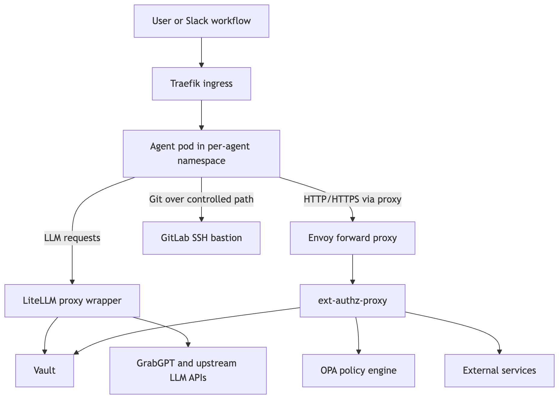
Kubernetes And Kernel Panics

Post Syndicated from Netflix Technology Blog original https://netflixtechblog.com/kubernetes-and-kernel-panics-ed620b9c6225

How Netflix’s Container Platform Connects Linux Kernel Panics to Kubernetes Pods

By Kyle Anderson

With a recent effort to reduce customer (engineers, not end users) pain on our container platform Titus, I started investigating “orphaned” pods. There are pods that never got to finish and had to be garbage collected with no real satisfactory final status. Our Service job (think ReplicatSet) owners don’t care too much, but our Batch users care a lot. Without a real return code, how can they know if it is safe to retry or not?

These orphaned pods represent real pain for our users, even if they are a small percentage of the total pods in the system. Where are they going, exactly? Why did they go away?

This blog post shows how to connect the dots from the worst case scenario (a kernel panic) through to Kubernetes (k8s) and eventually up to us operators so that we can track how and why our k8s nodes are going away.

Where Do Orphaned Pods Come From?

Orphaned pods get lost because the underlying k8s node object goes away. Once that happens a GC process deletes the pod. On Titus we run a custom controller to store the history of Pod and Node objects, so that we can save some explanation and show it to our users. This failure mode looks like this in our UI:

What it looks like to our users when a k8s node and its pods disappear

This is an explanation, but it wasn’t very satisfying to me or to our users. Why was the agent lost?

Where Do Lost Nodes Come From?

Nodes can go away for any reason, especially in “the cloud”. When this happens, usually a k8s cloud-controller provided by the cloud vendor will detect that the actual server, in our case an EC2 Instance, has actually gone away, and will in turn delete the k8s node object. That still doesn’t really answer the question of why.

How can we make sure that every instance that goes away has a reason, account for that reason, and bubble it up all the way to the pod? It all starts with an annotation:

{
"apiVersion": "v1",
"kind": "Pod",
"metadata": {
"annotations": {
"pod.titus.netflix.com/pod-termination-reason": "Something really bad happened!",
...

Just making a place to put this data is a great start. Now all we have to do is make our GC controllers aware of this annotation, and then sprinkle it into any process that could potentially make a pod or node go away unexpectedly. Adding an annotation (as opposed to patching the status) preserves the rest of the pod as-is for historical purposes. (We also add annotations for what did the terminating, and a short reason-code for tagging)

The pod-termination-reason annotation is useful to populate human readable messages like:

  • “This pod was preempted by a higher priority job ($id)”
  • “This pod had to be terminated because the underlying hardware failed ($failuretype)”
  • “This pod had to be terminated because $user ran sudo halt on the node”
  • “This pod died unexpectedly because the underlying node kernel panicked!”

But wait, how are we going to annotate a pod for a node that kernel panicked?

Capturing Kernel Panics

When the Linux kernel panics, there is just not much you can do. But what if you could send out some sort of “with my final breath, I curse Kubernetes!” UDP packet?

Inspired by this Google Spanner paper, where Spanner nodes send out a “last gasp” UDP packet to release leases & locks, you too can configure your servers to do the same upon kernel panic using a stock Linux module: netconsole.

Configuring Netconsole

The fact that the Linux kernel can even send out UDP packets with the string ‘kernel panic’, while it is panicking, is kind of amazing. This works because netconsole needs to be configured with almost the entire IP header filled out already beforehand. That is right, you have to tell Linux exactly what your source MAC, IP, and UDP Port are, as well as the destination MAC, IP, and UDP ports. You are practically constructing the UDP packet for the kernel. But, with that prework, when the time comes, the kernel can easily construct the packet and get it out the (preconfigured) network interface as things come crashing down. Luckily the netconsole-setup command makes the setup pretty easy. All the configuration options can be set dynamically as well, so that when the endpoint changes one can point to the new IP.

Once this is setup, kernel messages will start flowing right after modprobe. Imagine the whole thing operating like a dmesg | netcat -u $destination 6666, but in kernel space.

Netconsole “Last Gasp” Packets

With netconsole setup, the last gasp from a crashing kernel looks like a set of UDP packets exactly like one might expect, where the data of the UDP packet is simply the text of the kernel message. In the case of a kernel panic, it will look something like this (one UDP packet per line):

Kernel panic - not syncing: buffer overrun at 0x4ba4c73e73acce54
[ 8374.456345] CPU: 1 PID: 139616 Comm: insmod Kdump: loaded Tainted: G OE
[ 8374.458506] Hardware name: Amazon EC2 r5.2xlarge/, BIOS 1.0 10/16/2017
[ 8374.555629] Call Trace:
[ 8374.556147] <TASK>
[ 8374.556601] dump_stack_lvl+0x45/0x5b
[ 8374.557361] panic+0x103/0x2db
[ 8374.558166] ? __cond_resched+0x15/0x20
[ 8374.559019] ? do_init_module+0x22/0x20a
[ 8374.655123] ? 0xffffffffc0f56000
[ 8374.655810] init_module+0x11/0x1000 [kpanic]
[ 8374.656939] do_one_initcall+0x41/0x1e0
[ 8374.657724] ? __cond_resched+0x15/0x20
[ 8374.658505] ? kmem_cache_alloc_trace+0x3d/0x3c0
[ 8374.754906] do_init_module+0x4b/0x20a
[ 8374.755703] load_module+0x2a7a/0x3030
[ 8374.756557] ? __do_sys_finit_module+0xaa/0x110
[ 8374.757480] __do_sys_finit_module+0xaa/0x110
[ 8374.758537] do_syscall_64+0x3a/0xc0
[ 8374.759331] entry_SYSCALL_64_after_hwframe+0x62/0xcc
[ 8374.855671] RIP: 0033:0x7f2869e8ee69
...

Connecting to Kubernetes

The last piece is to connect is Kubernetes (k8s). We need a k8s controller to do the following:

  1. Listen for netconsole UDP packets on port 6666, watching for things that look like kernel panics from nodes.
  2. Upon kernel panic, lookup the k8s node object associated with the IP address of the incoming netconsole packet.
  3. For that k8s node, find all the pods bound to it, annotate, then delete those pods (they are toast!).
  4. For that k8s node, annotate the node and then delete it too (it is also toast!).

Parts 1&2 might look like this:

for {
n, addr, err := serverConn.ReadFromUDP(buf)
if err != nil {
klog.Errorf("Error ReadFromUDP: %s", err)
} else {
line := santizeNetConsoleBuffer(buf[0:n])
if isKernelPanic(line) {
panicCounter = 20
go handleKernelPanicOnNode(ctx, addr, nodeInformer, podInformer, kubeClient, line)
}
}
if panicCounter > 0 {
klog.Infof("KernelPanic context from %s: %s", addr.IP, line)
panicCounter++
}
}

And then parts 3&4 might look like this:

func handleKernelPanicOnNode(ctx context.Context, addr *net.UDPAddr, nodeInformer cache.SharedIndexInformer, podInformer cache.SharedIndexInformer, kubeClient kubernetes.Interface, line string) {
node := getNodeFromAddr(addr.IP.String(), nodeInformer)
if node == nil {
klog.Errorf("Got a kernel panic from %s, but couldn't find a k8s node object for it?", addr.IP.String())
} else {
pods := getPodsFromNode(node, podInformer)
klog.Infof("Got a kernel panic from node %s, annotating and deleting all %d pods and that node.", node.Name, len(pods))
annotateAndDeletePodsWithReason(ctx, kubeClient, pods, line)
err := deleteNode(ctx, kubeClient, node.Name)
if err != nil {
klog.Errorf("Error deleting node %s: %s", node.Name, err)
} else {
klog.Infof("Deleted panicked node %s", node.Name)
}
}
}

With that code in place, as soon as a kernel panic is detected, the pods and nodes immediately go away. No need to wait for any GC process. The annotations help document what happened to the node & pod:

A real pod lost on a real k8s node that had a real kernel panic!

Conclusion

Marking that a job failed because of a kernel panic may not be that satisfactory to our customers. But they can take satisfaction in knowing that we now have the required observability tools to start fixing those kernel panics!

Do you also enjoy really getting to the bottom of why things fail in your systems or think kernel panics are cool? Join us on the Compute Team where we are building a world-class container platform for our engineers.


Kubernetes And Kernel Panics was originally published in Netflix TechBlog on Medium, where people are continuing the conversation by highlighting and responding to this story.

Let’s Architect! Security in software architectures

Post Syndicated from Luca Mezzalira original https://aws.amazon.com/blogs/architecture/lets-architect-security-in-software-architectures/

Security is fundamental for each product and service you are building with. Whether you are working on the back-end or the data and machine learning components of a system, the solution should be securely built.

In 2022, we discussed security in our post Let’s Architect! Architecting for Security. Today, we take a closer look at general security practices for your cloud workloads to secure both networks and applications, with a mix of resources to show you how to architect for security using the services offered by Amazon Web Services (AWS).

In this edition of Let’s Architect!, we share some practices for protecting your workloads from the most common attacks, introduce the Zero Trust principle (you can learn how AWS itself is implementing it!), plus how to move to containers and/or alternative approaches for managing your secrets.

A deep dive on the current security threat landscape with AWS

This session from AWS re:Invent, security engineers guide you through the most common threat vectors and vulnerabilities that AWS customers faced in 2022. For each possible threat, you can learn how it’s implemented by attackers, the weaknesses attackers tend to leverage, and the solutions offered by AWS to avert these security issues. We describe this as fundamental architecting for security: this implies adopting suitable services to protect your workloads, as well as follow architectural practices for security.

Take me to this re:Invent 2022 session!

Statistics about common attacks and how they can be launched

Statistics about common attacks and how they can be launched

Zero Trust: Enough talk, let’s build better security

What is Zero Trust? It is a security model that produces higher security outcomes compared with the traditional network perimeter model.

How does Zero Trust work in practice, and how can you start adopting it? This AWS re:Invent 2022 session defines the Zero Trust models and explains how to implement one. You can learn how it is used within AWS, as well as how any architecture can be built with these pillars in mind. Furthermore, there is a practical use case to show you how Delphix put Zero Trust into production.

Take me to this re:Invent 2022 session!

AWS implements the Zero Trust principle for managing interactions across different services

AWS implements the Zero Trust principle for managing interactions across different services

A deep dive into container security on AWS

Nowadays, it’s vital to have a thorough understanding of a container’s underlying security layers. AWS services, like Amazon Elastic Kubernetes Service and Amazon Elastic Container Service, have harnessed these Linux security-layer protections, keeping a sharp focus on the principle of least privilege. This approach significantly minimizes the potential attack surface by limiting the permissions and privileges of processes, thus upholding the integrity of the system.

This re:Inforce 2023 session discusses best practices for securing containers for your distributed systems.

Take me to this re:Inforce 2023 session!

Fundamentals and best practices to secure containers

Fundamentals and best practices to secure containers

Migrating your secrets to AWS Secrets Manager

Secrets play a critical role in providing access to confidential systems and resources. Ensuring the secure and consistent management of these secrets, however, presents a challenge for many organizations.

Anti-patterns observed in numerous organizational secrets management systems include sharing plaintext secrets via unsecured means, such as emails or messaging apps, which can allow application developers to view these secrets in plaintext or even neglect to rotate secrets regularly. This detailed guidance walks you through the steps of discovering and classifying secrets, plus explains the implementation and migration processes involved in transferring secrets to AWS Secrets Manager.

Take me to this AWS Security Blog post!

An organization's perspectives and responsibilities when building a secrets management solution

An organization’s perspectives and responsibilities when building a secrets management solution

Conclusion

We’re glad you joined our conversation on building secure architectures! Join us in a couple of weeks when we’ll talk about cost optimization on AWS.

To find all the blogs from this series, visit the Let’s Architect! list of content on the AWS Architecture Blog.

Kubernetes monitoring with Zabbix – Part 3: Extracting Prometheus metrics with Zabbix preprocessing

Post Syndicated from Michaela DeForest original https://blog.zabbix.com/kubernetes-monitoring-with-zabbix-part-3-extracting-prometheus-metrics-with-zabbix-preprocessing/25639/

In the previous Kubernetes monitoring blog post, we explored the functionality provided by the Kubernetes integration in Zabbix and discussed use cases for monitoring and alerting to events in a cluster, such as changes in replicas or CPU pressure.

In the final part of this series on monitoring Kubernetes with Zabbix, we will show how the Kubernetes integration uses Prometheus to parse data from kube-state-metrics and how users can leverage this functionality to monitor the many cloud-native applications that expose Prometheus metrics by default.

Want to see Kubernetes monitoring in action? Watch Part 3 of our Kubernetes monitoring video guide.

Prometheus Data Model

Prometheus is an open-source toolkit for monitoring and alerting created by SoundCloud. Prometheus was the second hosted project to join the Cloud-native Computing Foundation in 2016, after Kubernetes. As such, users of Kubernetes have adopted Prometheus extensively.

Lines in the model begin with or without a pound sign. Lines beginning with a pound sign specify metadata that includes help text and type information. Additional lines follow where the first key is the metric name with optional labels specified, followed by the value, and optionally concluding with a timestamp. If a timestamp is absent, the assumption is that the timestamp is equal to the time of collection.

http_requests_total{job=”nginx”,instance=”10.0.0.1:443”} 15 1677507349983

Using Prometheus with Kubernetes Monitoring

Let’s start with an example from the kube-state-metrics endpoint, installed in the first part of this series. Below is the output for the /metrics endpoint used by the Kubernetes integration, showing the metric kube_job_created. Each metric has help text followed by a line starting with that metric name, labels describing each job, and creation time as the sample value.

# HELP kube_job_created Unix creation timestamp
# TYPE kube_job_created gauge
kube_job_created{namespace="jdoe",job_name="supportreport-supportreport-27956880"} 1.6774128e+09
kube_job_created{namespace="default",job_name="core-backup-data-default-0-27957840"} 1.6774704e+09
kube_job_created{namespace="default",job_name="core-backup-data-default-1-27956280"} 1.6773768e+09
kube_job_created{namespace="jdoe",job_name="activetrials-activetrials-27958380"} 1.6775028e+09
kube_job_created{namespace="default",job_name="core-cache-tags-27900015"} 1.6740009e+09
kube_job_created{namespace="default",job_name="core-cleanup-pipes-27954860"} 1.6772916e+09
kube_job_created{namespace="jdoe",job_name="salesreport-salesreport-27954060"} 1.6772436e+09
kube_job_created{namespace="default",job_name="core-correlation-cron-1671562914"} 1.671562914e+09
kube_job_created{namespace="jtroy",job_name="jtroy-clickhouse-default-0-maintenance-27613440"} 1.6568064e+09
kube_job_created{namespace="default",job_name="core-backup-data-default-0-27956880"} 1.6774128e+09
kube_job_created{namespace="default",job_name="core-cleanup-sessions-27896445"} 1.6737867e+09
kube_job_created{namespace="default",job_name="report-image-findings-report-27937095"} 1.6762257e+09
kube_job_created{namespace="jdoe",job_name="salesreport-salesreport-27933900"} 1.676034e+09
kube_job_created{namespace="default",job_name="core-cache-tags-27899775"} 1.6739865e+09
kube_job_created{namespace="ssmith",job_name="test-auto-merger"} 1.653574763e+09
kube_job_created{namespace="default",job_name="report-image-findings-report-1650569984"} 1.650569984e+09
kube_job_created{namespace="ssmith",job_name="auto-merger-and-mailer-auto-merger-and-mailer-27952200"} 1.677132e+09
kube_job_created{namespace="default",job_name="core-create-pipes-pxc-user"} 1.673279381e+09
kube_job_created{namespace="jdoe",job_name="activetrials-activetrials-1640610000"} 1.640610005e+09
kube_job_created{namespace="jdoe",job_name="salesreport-salesreport-27943980"} 1.6766388e+09
kube_job_created{namespace="default",job_name="core-cache-accounting-map-27958085"} 1.6774851e+09

Zabbix collects data from this endpoint in the “Get state metrics.” The item uses a script item type to get data from the /metrics endpoint. Dependent items that use a Prometheus pattern as a preprocessing step to obtain data relevant to the dependent item are created.

Prometheus and Out-Of-The-Box Templates

Zabbix also offers many templates for applications that expose Prometheus metrics, including etcd. Etcd is a distributed key-value store that uses a simple HTTP interface. Many cloud applications use etcd, including Kubernetes. Following is a description of how to set up an etcd “host” using the built-in etcd template.

A new host is created called “Etcd Application” with an agent interface specified that provides the location of the application API. The interface port does not matter because a macro sets the port. The “Etcd by HTTP” template is attached to the host.

The “Get node metrics” item is the master item that collects Prometheus metrics. Testing this item shows that it returns Prometheus formatted metrics. The master item creates many dependent items that parse the Prometheus metrics. In the dependent item, “Maximum open file descriptors,” the maximum number of open file descriptors is obtained by adding the “Prometheus pattern” preprocessing step. This metric is available with the metric name process_max_fds.

Custom Prometheus Templates


While it is convenient when Zabbix has a template for the application you want to monitor, creating a new template for an application that exposes a /metrics endpoint but does not have an associated template is easy.

One such application is Argo CD. Argo CD is a GitOps continuous delivery tool for Kubernetes. An “application” represents each deployment in Kubernetes. Argo CD uses Git to keep applications in sync.

Argo CD exposes a Prometheus metrics endpoint that we can be used to monitor the application. The Argo CD documentation site includes information about available metrics.

In Argo CD, the metrics service is available at the argocd-metrics service. Following is a demonstration of creating an Argo CD template that collects Prometheus metrics. Install Argo CD in a cluster with a Zabbix proxy installed before starting. To do this, follow the Argo CD “Getting Started” guide.

Create a new template called, “Argo CD by HTTP” in the “Templates/Applications” group. Add three macros to the template. Set {$ARGO.METRICS.SERVICE.PORT} to the default of 8082. Set {$ARGO.METRICS.API.PATH} to “/metrics.” Set the last macro, {$ARGO.METRICS.SCHEME} to the default of “http.”

Open the template and click “Items -> Create item.” Name this item “Get Application Metrics” and give it the “HTTP agent” type. Set the key to argocd.get_metrics with a “Text” information type. Set the URL to {$ARGO.METRICS.SCHEME}://{HOST.CONN}:{$ARGO.METRICS.SERVICE.PORT}/metrics. Set the History storage period to “Do not keep history.”

Create a new host to represent Argo. Go to “Hosts -> Create host”. Name the host “Argo CD Application” and assign the newly created template. Define an interface and set the DNS name to the name of the metrics service, including the namespace, if the Argo CD deployment is not in the same namespace as the Zabbix proxy deployment. Connect to DNS and leave the port as the default because the template does not use this value. Like in the etcd template, a macro sets the port. Set the proxy to the proxy located in the cluster. In most cases, the macros do not need to be updated.

Click “Test -> Get value and test” to test the item. Prometheus metrics are returned, including a metric called argocd_app_info. This metric collects the status of the applications in Argo. We can collect all deployed applications with a discovery rule.

Navigate to the Argo CD template and click “Discovery rules -> Create discovery rule.” Call the rule “Discover Applications.” The type should be “Dependent item” because it depends on the metrics collection item. Set the master item to the “Get Application Metrics” item. The key will be argocd.applications.discovery. Go to the preprocessing tab and add a new step called, “Prometheus to JSON.” The preprocessing step will convert the application data to JSON, which will look like the one below.

[{"name":"argocd_app_info","value":"1","line_raw":"argocd_app_info{dest_namespace=\"monitoring\",dest_server=\"https://kubernetes.default.svc\",health_status=\"Healthy\",name=\"guestbook\",namespace=\"argocd\",operation=\"\",project=\"default\",repo=\"https://github.com/argoproj/argocd-example-apps\",sync_status=\"Synced\"} 1","labels":{"dest_namespace":"monitoring","dest_server":"https://kubernetes.default.svc","health_status":"Healthy","name":"guestbook","namespace":"argocd","operation":"","project":"default","repo":"https://github.com/argoproj/argocd-example-apps","sync_status":"Synced"},"type":"gauge","help":"Information about application."}]

Set the parameters to “argocd_app_info” to gather all metrics with that name. Under “LLD Macros”, set three macros. {#NAME} is set to the .labels.name key, {#NAMESPACE} is set to the .labels.dest_namespace key, and {#SERVER} is set to .labels.dest_server.

Let us create some item prototypes. Click “Create item prototype” and name it “{#NAME}: Health Status.” Set it as a dependent item with a key of argocd.applications[{#NAME}].health. The type of information will be “Character.” Set the master item to “Get Application Metrics.”

In preprocessing, add a Prometheus pattern step with parameters argocd_app_info{name=”{#NAME}”}. Use “label” and set the label to health_status. Add a second step to “Discard unchanged with heartbeat” with the heartbeat set to 2h.

Clone the prototype to create another item called “{#NAME}: Sync status.” Change the key to argocd.applications.sync[{#NAME}]. Under “Preprocessing” change the label to sync_status.

Now, when viewing “Latest Data” the sync and health status are available for each discovered application.

Conclusion

We have shown how Zabbix templates, such as the Kubernetes template, and the etcd template utilize Prometheus patterns to extract metric data. We have also created templates for new applications that expose Prometheus data. Because of the adoption of Prometheus in Kubernetes and cloud-native applications, Zabbix benefits by parsing this data so that Zabbix can monitor Kubernetes and cloud-native applications.

I hope you enjoyed this series on monitoring Kubernetes and cloud-native applications with Zabbix. Good luck on your monitoring journey as you learn to monitor with Zabbix in a containerized world.

About the Author

Michaela DeForest is a Platform Engineer for The ATS Group. She is a Zabbix Certified Specialist on Zabbix 6.0 with additional areas of expertise, including Terraform, Amazon Web Services (AWS), Ansible, and Kubernetes, to name a few. As ATS’s resident authority in DevOps, Michaela is critical in delivering cutting-edge solutions that help businesses improve efficiency, reduce errors, and achieve a faster ROI.

About ATS Group:

The ATS Group provides a fully inclusive set of technology services and tools designed to innovate and transform IT. Their systems integration, business resiliency, cloud enablement, infrastructure intelligence, and managed services help businesses of all sizes “get IT done.” With over 20 years in business, ATS has become the trusted advisor to nearly 500 customers across multiple industries. They have built their reputation around honesty, integrity, and technical expertise unrivaled by the competition.

Kubernetes monitoring with Zabbix – Part 2: Understanding the discovered resources

Post Syndicated from Michaela DeForest original https://blog.zabbix.com/kubernetes-monitoring-with-zabbix-part-2-understanding-the-discovered-resources/25476/

In the previous blog post, we installed the Zabbix Agent Helm Chart and set up official Kubernetes templates to monitor a cluster in Zabbix. In this edition, part 2, we will explore the functionality provided by the Kubernetes integration in Zabbix and discuss use cases for monitoring and alerting on events in a cluster. (This post assumes that the Kubernetes integration has been set up in at least one cluster using the helm chart and provided templates.)

Want to see Kubernetes monitoring in action? Watch Part 2 of our Kubernetes monitoring video guide.

Node and Component Discovery

Following integration setup, the templates will discover control plane components, each node, and the kubelet associated with it using the Kubernetes API via a “Script” item type.

Note:

In the last blog post, I showed a managed EKS cluster. Control plane components cannot be discovered in an EKS cluster because AWS does not make them directly available through the API. For the sake of demonstrating the full capabilities of the integration, this post will use screenshots depicting a cluster that was created using the kubeadm utility.

In the latest version of Zabbix (6.2 at the time of writing), control plane components are discovered via node labels added only for clusters created with kubeadm. Depending on your setup, you may be able to add the same node labels to your own control plane nodes or modify the template to use your specific labels.

This example cluster has 4 worker nodes and 1 master node. The control plane runs entirely on the master node.

Zabbix’s “Low-Level Discovery” is the backbone of the Kubernetes integration. Zabbix discovers each node and creates two hosts to represent them in the cluster. The first host attaches the “Linux by Zabbix Agent” template to it, and the second attaches a custom Kubelet template called “Kubernetes Kubelet by HTTP. Zabbix also creates items for most standard objects like pods, deployments, replicasets, job, cronjob, etc.

Node and Kubernetes Performance Metrics

In this example, there are four discovered worker nodes with the “Linux by Zabbix Agent” template attached to them. The template will provide metrics about the machines running in the cluster.

Each worker host’s “System performance” dashboard shows system load, CPU usage, and memory usage metrics.

Zabbix will also collect Kubernetes-specific metrics related to the nodes. “Latest Data” for the Kubernetes Nodes host shows metrics such as the Allocatable CPU available to pods and the node’s memory capacity.

Alerts are generated for events such as the allocation of too much CPU. This could indicate that capacity should be increased, assuming that the memory and CPU limits set on the pod label are accurate.

The Kubernetes integration also monitors object states. As a best practice, any tool used to monitor Kubernetes should be monitoring and alerting critical status changes within the cluster. The image above shows the triggers related to the health of a pod. There are also triggers when certain conditions are detected by the nodes, like memory or CPU pressure.

Zabbix discovers objects like pods, deployments, and Replicasets, and triggers on object states.  For example, pods that are not up or deployments that do not have the correct number of replicas up.

In this example, a cluster is running a Kubernetes dashboard deployment with 3 replicas. By running the following command, we can see that all 3 replicas are up. Under “Latest Data,” Zabbix shows those 3 replicas available out of the 3 desired.

kubectl get deployment kubernetes-dashboard


To mimic a pod crashing, the pod is edited to use an invalid image tag.

kubectl edit pod <pod name>

The image tag is changed to  “invalid.tag, “ which is unavailable for the image. This causes the pod to fail because it can no longer pull the image. Output now shows that one pod is no longer ready.

Looking at the data in Zabbix, the number of available replicas is only 3, while the number of unavailable replicas is now 1.

On the problems page, there are two new problems. Both alerted that there is a mismatch between the number of replicas for the dashboard and the number of desired replicas.

Changing the tag back to a valid one should cause those problems to be resolved.

The Kubernetes templates offer many metrics and triggers, including most provided by Prometheus and Alert Manager. With some Zabbix experience and the ability to navigate kube-state-metrics and Kubernetes APIs, creating new items is possible.

What’s Next?

Above is an example of the output from the kube-state-metrics API. Unlike most APIs that return data in JSON format, the kube-state-metrics API uses the Prometheus data model to supply metrics.

As you get comfortable with Kubernetes monitoring in Zabbix, you may want to parse your own metrics from kube-state-metrics and create new items.

In the next video, we will learn how to monitor applications with Prometheus in Zabbix.

About the Author

Michaela DeForest is a Platform Engineer for The ATS Group.  She is a Zabbix Certified Specialist on Zabbix 6.0 with additional areas of expertise, including Terraform, Amazon Web Services (AWS), Ansible, and Kubernetes, to name a few.  As ATS’s resident authority in DevOps, Michaela is critical in delivering cutting-edge solutions that help businesses improve efficiency, reduce errors, and achieve a faster ROI.

About ATS Group: The ATS Group provides a fully inclusive set of technology services and tools designed to innovate and transform IT.  Their systems integration, business resiliency, cloud enablement, infrastructure intelligence, and managed services help businesses of all sizes “get IT done.” With over 20 years in business, ATS has become the trusted advisor to nearly 500 customers across multiple industries.  They have built their reputation around honesty, integrity, and technical expertise unrivaled by the competition.

Intelligent, automatic restarts for unhealthy Kafka consumers

Post Syndicated from Chris Shepherd original https://blog.cloudflare.com/intelligent-automatic-restarts-for-unhealthy-kafka-consumers/

Intelligent, automatic restarts for unhealthy Kafka consumers

Intelligent, automatic restarts for unhealthy Kafka consumers

At Cloudflare, we take steps to ensure we are resilient against failure at all levels of our infrastructure. This includes Kafka, which we use for critical workflows such as sending time-sensitive emails and alerts.

We learned a lot about keeping our applications that leverage Kafka healthy, so they can always be operational. Application health checks are notoriously hard to implement: What determines an application as healthy? How can we keep services operational at all times?

These can be implemented in many ways. We’ll talk about an approach that allows us to considerably reduce incidents with unhealthy applications while requiring less manual intervention.

Kafka at Cloudflare

Cloudflare is a big adopter of Kafka. We use Kafka as a way to decouple services due to its asynchronous nature and reliability. It allows different teams to work effectively without creating dependencies on one another. You can also read more about how other teams at Cloudflare use Kafka in this post.

Kafka is used to send and receive messages. Messages represent some kind of event like a credit card payment or details of a new user created in your platform. These messages can be represented in multiple ways: JSON, Protobuf, Avro and so on.

Kafka organises messages in topics. A topic is an ordered log of events in which each message is marked with a progressive offset. When an event is written by an external system, that is appended to the end of that topic. These events are not deleted from the topic by default (retention can be applied).

Intelligent, automatic restarts for unhealthy Kafka consumers

Topics are stored as log files on disk, which are finite in size. Partitions are a systematic way of breaking the one topic log file into many logs, each of which can be hosted on separate servers–enabling to scale topics.

Topics are managed by brokers–nodes in a Kafka cluster. These are responsible for writing new events to partitions, serving reads and replicating partitions among themselves.

Messages can be consumed by individual consumers or co-ordinated groups of consumers, known as consumer groups.

Consumers use a unique id (consumer id) that allows them to be identified by the broker as an application which is consuming from a specific topic.

Each topic can be read by an infinite number of different consumers, as long as they use a different id. Each consumer can replay the same messages as many times as they want.

When a consumer starts consuming from a topic, it will process all messages, starting from a selected offset, from each partition. With a consumer group, the partitions are divided amongst each consumer in the group. This division is determined by the consumer group leader. This leader will receive information about the other consumers in the group and will decide which consumers will receive messages from which partitions (partition strategy).

Intelligent, automatic restarts for unhealthy Kafka consumers

The offset of a consumer’s commit can demonstrate whether the consumer is working as expected. Committing a processed offset is the way a consumer and its consumer group report to the broker that they have processed a particular message.

Intelligent, automatic restarts for unhealthy Kafka consumers

A standard measurement of whether a consumer is processing fast enough is lag. We use this to measure how far behind the newest message we are. This tracks time elapsed between messages being written to and read from a topic. When a service is lagging behind, it means that the consumption is at a slower rate than new messages being produced.

Due to Cloudflare’s scale, message rates typically end up being very large and a lot of requests are time-sensitive so monitoring this is vital.

At Cloudflare, our applications using Kafka are deployed as microservices on Kubernetes.

Health checks for Kubernetes apps

Kubernetes uses probes to understand if a service is healthy and is ready to receive traffic or to run. When a liveness probe fails and the bounds for retrying are exceeded, Kubernetes restarts the services.

Intelligent, automatic restarts for unhealthy Kafka consumers

When a readiness probe fails and the bounds for retrying are exceeded, it stops sending HTTP traffic to the targeted pods. In the case of Kafka applications this is not relevant as they don’t run an http server. For this reason, we’ll cover only liveness checks.

A classic Kafka liveness check done on a consumer checks the status of the connection with the broker. It’s often best practice to keep these checks simple and perform some basic operations – in this case, something like listing topics. If, for any reason, this check fails consistently, for instance the broker returns a TLS error, Kubernetes terminates the service and starts a new pod of the same service, therefore forcing a new connection. Simple Kafka liveness checks do a good job of understanding when the connection with the broker is unhealthy.

Intelligent, automatic restarts for unhealthy Kafka consumers

Problems with Kafka health checks

Due to Cloudflare’s scale, a lot of our Kafka topics are divided into multiple partitions (in some cases this can be hundreds!) and in many cases the replica count of our consuming service doesn’t necessarily match the number of partitions on the Kafka topic. This can mean that in a lot of scenarios this simple approach to health checking is not quite enough!

Microservices that consume from Kafka topics are healthy if they are consuming and committing offsets at regular intervals when messages are being published to a topic. When such services are not committing offsets as expected, it means that the consumer is in a bad state, and it will start accumulating lag. An approach we often take is to manually terminate and restart the service in Kubernetes, this will cause a reconnection and rebalance.

Intelligent, automatic restarts for unhealthy Kafka consumers

When a consumer joins or leaves a consumer group, a rebalance is triggered and the consumer group leader must re-assign which consumers will read from which partitions.

When a rebalance happens, each consumer is notified to stop consuming. Some consumers might get their assigned partitions taken away and re-assigned to another consumer. We noticed when this happened within our library implementation; if the consumer doesn’t acknowledge this command, it will wait indefinitely for new messages to be consumed from a partition that it’s no longer assigned to, ultimately leading to a deadlock. Usually a manual restart of the faulty client-side app is needed to resume processing.

Intelligent health checks

As we were seeing consumers reporting as “healthy” but sitting idle, it occurred to us that maybe we were focusing on the wrong thing in our health checks. Just because the service is connected to the Kafka broker and can read from the topic, it does not mean the consumer is actively processing messages.

Therefore, we realised we should be focused on message ingestion, using the offset values to ensure that forward progress was being made.

The PagerDuty approach

PagerDuty wrote an excellent blog on this topic which we used as inspiration when coming up with our approach.

Their approach used the current (latest) offset and the committed offset values. The current offset signifies the last message that was sent to the topic, while the committed offset is the last message that was processed by the consumer.

Intelligent, automatic restarts for unhealthy Kafka consumers

Checking the consumer is moving forwards, by ensuring that the latest offset was changing (receiving new messages) and the committed offsets were changing as well (processing the new messages).

Therefore, the solution we came up with:

  • If we cannot read the current offset, fail liveness probe.
  • If we cannot read the committed offset, fail liveness probe.
  • If the committed offset == the current offset, pass liveness probe.
  • If the value for the committed offset has not changed since the last run of the health check, fail liveness probe.
Intelligent, automatic restarts for unhealthy Kafka consumers

To measure if the committed offset is changing, we need to store the value of the previous run, we do this using an in-memory map where partition number is the key. This means each instance of our service only has a view of the partitions it is currently consuming from and will run the health check for each.

Problems

When we first rolled out our smart health checks we started to notice cascading failures some time after release. After initial investigations we realised this was happening when a rebalance happens. It would initially affect one replica then quickly result in the others reporting as unhealthy.

What we observed was due to us storing the previous value of the committed offset in-memory, when a rebalance happens the service may get re-assigned a different partition. When this happened it meant our service was incorrectly assuming that the committed offset for that partition had not changed (as this specific replica was no longer updating the latest value), therefore it would start to report the service as unhealthy. The failing liveness probe would then cause it to restart which would in-turn trigger another rebalancing in Kafka causing other replicas to face the same issue.

Solution

To fix this issue we needed to ensure that each replica only kept track of the offsets for the partitions it was consuming from at that moment. Luckily, the Shopify Sarama library, which we use internally, has functionality to observe when a rebalancing happens. This meant we could use it to rebuild the in-memory map of offsets so that it would only include the relevant partition values.

This is handled by receiving the signal from the session context channel:

for {
  select {
  case message, ok := <-claim.Messages(): // <-- Message received

     // Store latest received offset in-memory
     offsetMap[message.Partition] = message.Offset


     // Handle message
     handleMessage(ctx, message)


     // Commit message offset
     session.MarkMessage(message, "")


  case <-session.Context().Done(): // <-- Rebalance happened

     // Remove rebalanced partition from in-memory map
     delete(offsetMap, claim.Partition())
  }
}

Verifying this solution was straightforward, we just needed to trigger a rebalance. To test this worked in all possible scenarios we spun up a single replica of a service consuming from multiple partitions, then proceeded to scale up the number of replicas until it matched the partition count, then scaled back down to a single replica. By doing this we verified that the health checks could safely handle new partitions being assigned as well as partitions being taken away.

Takeaways

Probes in Kubernetes are very easy to set up and can be a powerful tool to ensure your application is running as expected. Well implemented probes can often be the difference between engineers being called out to fix trivial issues (sometimes outside of working hours) and a service which is self-healing.

However, without proper thought, “dumb” health checks can also lead to a false sense of security that a service is running as expected even when it’s not. One thing we have learnt from this was to think more about the specific behaviour of the service and decide what being unhealthy means in each instance, instead of just ensuring that dependent services are connected.

Monitoring Kubernetes with Zabbix

Post Syndicated from Michaela DeForest original https://blog.zabbix.com/monitoring-kubernetes-with-zabbix/25055/

There are many options available for monitoring Kubernetes and cloud-native applications. In this multi-part blog series, we’ll explore how to use Zabbix to monitor a Kubernetes cluster and understand the metrics generated within Zabbix. We’ll also learn how to exploit Prometheus endpoints exposed by applications to monitor application-specific metrics.

Want to see Kubernetes monitoring in action? Watch the step-by-step Zabbix Kubernetes monitoring configuration and deployment guide.

Why Choose Zabbix to Monitor Kubernetes?

Before choosing Zabbix as a Kubernetes monitoring tool, we asked ourselves, “why would we choose to use Zabbix rather than Prometheus, Grafana, and alertmanager?” After all, they have become the standard monitoring tools in the cloud ecosystem. We decided that our minimum criteria for Zabbix would be that it was just as effective as Prometheus for monitoring both Kubernetes and cloud-native applications.

Through our discovery process, we concluded that Zabbix meets (and exceeds) this minimum requirement. Zabbix provides similar metrics and triggers as Prometheus, alert manager, and Grafana for Kubernetes, as they both use the same backend tools to do this. However, Zabbix can do this in one product while still maintaining flexibility and allowing you to monitor pretty much anything you can write code to collect. Regarding application monitoring, Zabbix can transform Prometheus metrics fed to it by Prometheus exporters and endpoints. In addition, because Zabbix can make calls to any HTTP endpoint, it can monitor applications that do not have a dedicated Prometheus endpoint, unlike Prometheus.

The Zabbix Helm Chart

Zabbix monitors Kubernetes by collecting metrics exposed via the Kubernetes API and kube-state-metrics. The components necessary to monitor a cluster are installed within the cluster using this helm chart provided by Zabbix. The helm chart includes the Zabbix agent installed as a daemon set and is used to monitor local resources and applications on each node. A Zabbix proxy is also installed to collect monitoring data and transfer it to the external Zabbix server.

Only the Zabbix proxy needs access to the Zabbix server, while the agents can send data to the proxy installed in the same namespace as each agent. A cluster role allows Zabbix to access resources in the cluster via the Kubernetes API. While the cluster role could be modified to restrict privileges given to Zabbix, this will result in some items becoming unsupported. We recommend keeping this the same if you want to get the most out of Kubernetes monitoring with Zabbix.

The Zabbix helm chart installs the kube-state-metrics project as a dependency. You may already be familiar with this project under the Kubernetes organization, which generates Prometheus format metrics based on the current state of the Kubernetes resources. In addition, if you have experience using Prometheus to monitor a cluster, you may already have this installed. If that is the case, you can point to this deployment rather than installing another one.

In this tutorial, we will install kube-state-metrics via the Zabbix helm chart.

For more information on skipping this step, refer to the values file in the Zabbix Kubernetes helm chart.

Installing the Zabbix Helm Chart

Now that we’ve explained how the Zabbix helm chart works, let’s go ahead and install it. In this example, we will assume that you have a running Zabbix 6.0 (or higher) instance that is reachable from the cluster you wish to monitor. I am running a 6.0 instance in a different cluster than the one we want to monitor. The server is reachable via the DNS name mdeforest.zabbix.atsgroup.io with a non-standard port of 31103.

We will start by installing the latest Zabbix helm chart. I recommend visiting zabbix.com/integrations/kubernetes to get any sources that may be referred to in this tutorial. There you will find a link to the Zabbix helm chart and templates. For the most part, we will follow the steps outlined in the readme.


Using a terminal window, I am going to make sure the active cluster is set to the cluster that I want to monitor:

kubectl config use-context <cluster context name>

I’m then going to add the Zabbix chart repo to my local helm repository:

helm repo add zabbix-chart-6.0 https://cdn.zabbix.com/zabbix/integrations/kubernetes-helm/6.0/

If you’re running Zabbix 6.2 or newer, change the references to 6.0 in this command to 6.2.

Depending on your circumstances, you will need to set a few values for the installation. In most cases, you only need to set a few environment variables for the Zabbix agent and the proxy. The complete list of values and environment variables is available in the helm chart repo, alongside the agent and proxy images on Docker Hub.

In this case, I’m setting the passive server environment variable for the agent to allow any IP to connect. For the proxy, I am setting the server host accessible from the proxy alongside the non-standard port. I’ve also set here some variables related to cache size. These variables may depend on your cluster size, so you may need to play around with them to find the correct values.

Now that I have the values file ready, I’m ready to install the chart. So, we’ll use the following command. Of course, the chart path might vary depending on what version of the chart you’re using.

helm install -f </path/to/values/file> [-n <namespace>] zabbix zabbix-chart-6.0/zabbix-helm-chart

You can also optionally add a namespace. You must wait until everything is running, so I’ll check just that with the following:

watch kubectl get pods

Now that everything is installed, we’re ready to set up hosts in Zabbix that will be associated with the cluster. The last step before we have all the information we need is to obtain the token created via the service account installed with the helm chart. We’ll get this by running the next command, which is the name of the service account that was created:

kubectl get secret -o jsonpath={.data.token} zabbix service-account | base64 -d

This will get the secret created for the service account and grab just the token from that, which is passed to the base64 utility to decode it. Be sure to copy that value somewhere because you’ll need it for later.

You’ll also need the Kubernetes API endpoint. In most cases, you’ll use the proxy installed rather than the server directly or a proxy outside the cluster. If this is the case, you can use the service DNS for the API. We should be able to reach it by pointing to https://kubernetes.default.svc.cluster.local:443/api.

If this is not the case, you can use the output from the command:
kubectl cluster-info

Now, let’s head over to the Zabbix UI. All the templates we need are shipped in Zabbix 6. If for some reason, you can’t find them, they are available for download and import by visiting the integrations page that I pointed out earlier on the Zabbix site.

Adding the Proxy

We will add our proxy by heading to Administration -> Proxies:

  1. Click Create Proxy. Because this is an active proxy by default, we only need to specify the proxy name. If you didn’t make any changes to the helm chart, this should default to zabbix-proxy. If you’d like to name this differently, you can change the environment variable zbx_hostname for the proxy in the helm chart. We’re going to leave it as the default for now. You’re going to enter this name and then click “Add.” After a few minutes, you’ll start to see that it says that the proxy has been seen.
  2. Create a Host Group to put hosts related to Kubernetes. For this example, let’s create one, which we’ll call Kubernetes.
  3. Head to the host page under configuration and click Create Host. The first host will collect metrics related to monitoring Kubernetes nodes, and we’ll discover nodes and create new hosts using Zabbix low-level discovery.
  4. Give this host the name Kubernetes Nodes. We’ll also assign this host to the Kubernetes host group we created and attach the template Kubernetes nodes by HTTP.
  5. Change the line “Monitored by proxy” to the proxy created earlier, called zabbix-proxy.
  6. Click the Macros tab and select “Inherited and host macros.” You should be able to see all the macros that may be set to influence what is monitored in your cluster. In this case, we need to change the first two macros. The first, {KUBE.API.ENDPOINT.URL}, should be set to the Kubernetes API endpoint. In our case, we can set it to what I mentioned earlier: default.svc.cluster.local:443/api. Next, the token should be set to the previously retrieved value from the command line.
  7. lick Add. After a few minutes, you should start seeing data on the latest data page and new hosts on the host page representing each node.

Creating an Additional Host

Now let’s create another host that will represent the metrics available via the Kubernetes API and the kube-state-metrics endpoint.

  1. Click Create Host again, name this host Kubernetes Cluster State, and add it to the Kubernetes group again.
  2. Let’s also attach the Kubernetes Cluster State template by HTTP. Again, we’re going to choose the proxy that we created earlier.
  3. In the Macro section, change the kube.api.url to the same thing we used before, but this time leave off the /api at the end. Simply: default.svc.cluster.local:443. Be sure to set the token as we did before.
  4. Assuming nothing else was changed in the installation of the helm chart, we can now add that host.

After a few minutes, you should receive metrics related to the cluster state, including hosts representing the kubelet on each node.

What’s Next?

Now you’re all set to start monitoring your Kubernetes cluster in Zabbix! Give it a try, and let us know your thoughts in the comments.

In the next blog post, we’ll look at what you can do with your newly monitored cluster and how to get the most out of it.

If you’d like help with any of this, ATS has advanced monitoring, orchestration, and automation skills to make this process a snap. Set up a 15-minute with our team to go through any questions you have.

About the Author

Michaela DeForest is a Platform Engineer for The ATS Group.  She is a Zabbix Certified Specialist on Zabbix 6.0 with additional areas of expertise, including Terraform, Amazon Web Services (AWS), Ansible, and Kubernetes, to name a few.  As ATS’s resident authority in DevOps, Michaela is critical in delivering cutting-edge solutions that help businesses improve efficiency, reduce errors, and achieve a faster ROI.

About ATS Group: The ATS Group provides a fully inclusive set of technology services and tools designed to innovate and transform IT.  Their systems integration, business resiliency, cloud enablement, infrastructure intelligence, and managed services help businesses of all sizes “get IT done.” With over 20 years in business, ATS has become the trusted advisor to nearly 500 customers across multiple industries.  They have built their reputation around honesty, integrity, and technical expertise unrivaled by the competition.

How to investigate and take action on security issues in Amazon EKS clusters with Amazon Detective – Part 2

Post Syndicated from Marshall Jones original https://aws.amazon.com/blogs/security/how-to-investigate-and-take-action-on-security-issues-in-amazon-eks-clusters-with-amazon-detective-part-2/

In part 1 of this of this two-part series, How to detect security issues in Amazon EKS cluster using Amazon GuardDuty, we walked through a real-world observed security issue in an Amazon Elastic Kubernetes Service (Amazon EKS) cluster and saw how Amazon GuardDuty detected each phase by following MITRE ATT&CK tactics.

In this blog post, we’ll walk you through investigative techniques to use with Amazon Detective, paired with the GuardDuty EKS and malware findings from the security issue. After we have identified impacted resources through our investigation, we’ll provide example remediation tactics and preventative controls to address and help prevent security issues in EKS clusters.

Amazon Detective can help you investigate security issues and related resources in your account. Detective provides EKS coverage that you can enable within your accounts. When this coverage is enabled, Detective can help investigate and remediate potentially unauthorized EKS activity that results from misconfiguration of the control plane nodes or application. Although GuardDuty is not a prerequisite to enable Detective, it is recommended that you enable GuardDuty to enhance the visualization capabilities in Detective with GuardDuty findings.

Prerequisites

You must have the following services enabled in your AWS account to generate and investigate findings associated with EKS security events in a similar manner as outlined in this blog. If you do not have GuardDuty enabled, you can still investigate with Detective, but in a limited capacity.

Investigate with Amazon Detective

In the five phases we walked through in part 1, we discussed GuardDuty findings and MITRE ATT&CK tactics that can help you detect and understand each phase of the unauthorized activity, from the initial misconfiguration to the impact on our application when the EKS cluster is used for crypto mining.

The next recommended step is to investigate the EKS cluster and any associated resources. Amazon Detective can help you to investigate whether there was any other related unauthorized activity in the environment. We will walk through Detective capabilities for visualizing and gathering important information to effectively respond to the security issue. If you’re interested in creating detailed incident response playbooks for your security team to follow in your own environment, refer to these sample AWS incident response playbooks.

Depending on your scenario, there are various resources you can use to start your investigation, such as Security Hub findings, GuardDuty findings, related Kubernetes subjects, or an AWS account’s AWS CloudTrail activity. For our walkthrough, we’ll start our investigation from the GuardDuty finding and use the EKS cluster resource to pivot to the Detective console, as shown in Figure 7. Although we initially focus on the EKS cluster, you could start from any entities that are supported in the Detective behavior graph structure in the Amazon Detective User Guide. For example, we could start directly with the Kubernetes subject system:anonymous and find activity associated with the anonymous user.

Figure 7: Example Detective popup from GuardDuty finding for EKS cluster

Figure 7: Example Detective popup from GuardDuty finding for EKS cluster

We’ll now go over the information that you would need to gather from Detective in order to investigate the example security issue.

To investigate EKS cluster findings with Detective

  1. In the GuardDuty console, navigate to an individual finding and hover over Investigate with Detective. Choose one of the specific resources to start. In the image below, we selected the EKS cluster resource to investigate with Detective. You will need to gather some preliminary information about the IAM roles associated with the EKS cluster.
    • Questions: When was the cluster created? What IAM role created the cluster? What IAM role is assigned to the cluster?
    • Why it matters: If you are an incident responder, these details can potentially help you identify the owner of the cluster and help you determine what IAM principals are involved.
    • What next: Start looking into each IAM principal’s activity, as seen in CloudTrail, to investigate whether the IAM entity itself is potentially compromised or what other resources may have been impacted.
    Figure 8: Detective summary page for EKS cluster metadata details

    Figure 8: Detective summary page for EKS cluster metadata details

  2. Next, on the EKS cluster overview page, you can see the container details associated with the cluster.
    • Question: What are some of the other container details for the cluster? Does anything look out of the ordinary? Is it using a public image? Is it missing a network policy?
    • Why it matters: Based on the architecture related to this cluster, you might be able to use this information to determine whether there are unauthorized containers. The contents of unauthorized containers will depend on your organization but typically consist of public images or unauthorized RBAC, pod security policies, or network policy configurations. It’s important to keep in mind that when you look at data in Detective, the scope time is very important. When you pivot from a GuardDuty finding, the scope time will be set to the first time the GuardDuty finding was seen to the last time the finding was seen. The container details reflect the containers that were running during the selected scope time. Changing the scope time might change the containers that are listed in the table shown in Figure 9.
    • What next: Information found on this page can help to highlight unauthorized resources or configurations that will need to be remediated. You will also need to look at how these resources were initially created and if there are missing guardrails that should have been created during the provisioning of the cluster.
    Figure 9: Detective summary page for EKS container metadata details

    Figure 9: Detective summary page for EKS container metadata details

  3. Finally, you will see associated security findings with this specific EKS cluster, similar to Figure 10, at the bottom of the EKS cluster overview page in Detective.
    • Question: Are there any other security findings associated with this cluster that I previously was not aware of?
    • Why it matters: In our example scenario, we walked through the findings that were initially detected and the events that unfolded from those findings. After further investigation, you might see other findings that were not part of the original investigation. This can occur if your security team is only investigating specific findings or severity values. The finding for PrivilegeEscalation:Kubernetes/PrivilegedContainer informs you that a privileged container was launched on your Kubernetes cluster by using an image that has never before been used to launch privileged containers in your cluster. A privileged container has root level access to the host. The other finding, Persistence:Kubernetes/ContainerWithSensitiveMount, informs you that a container was launched with a configuration that included a sensitive host path with write access in the volumeMounts section. This makes the sensitive host path accessible and writable from inside the container. Any finding associated to the suspicious or compromised cluster is valuable because it provides additional insight into what the unauthorized entity was trying to accomplish after the initial detection.
    • What next: With Detective, you might want to continue your investigation by selecting each of these findings and reviewing all details related to the finding. Depending on the findings, you could bring in additional team members to help investigate further. For this example, we will move on to the next step.
    Figure 10: Example Detective summary of security findings associated with the EKS cluster

    Figure 10: Example Detective summary of security findings associated with the EKS cluster

  4. Shift from the EKS cluster overview section to the Kubernetes API activity section, similar to Figure 11 below. This will give you the opportunity to dig into the API activity associated with this cluster.
    1. Question: What other Kubernetes API activity was attempted from the cluster? Which API calls were successful? Which API calls failed? What was the unauthorized user trying to do?
    2. Why it matters: It’s important to determine which actions were successfully invoked by the unauthorized user so that appropriate remediation actions can be taken. You can look at trends of successful and failed API calls, and can even search by Subject, IP address, or Kubernetes API call.
    3. What next: You might want to look at all cluster role binding from days before the first GuardDuty finding was seen to determine if there was any other suspicious activity you should be investigating regarding the cluster.
    Figure 11: Example Detective summary page for Kubernetes API activity on the EKS cluster

    Figure 11: Example Detective summary page for Kubernetes API activity on the EKS cluster

  5. Next, you will want to look at the Newly observed Kubernetes API calls section, similar to Figure 12 below.
    • Question: What are some of the more recent Kubernetes API calls? What are they trying to access right now and are they successful? Do I need to start taking action for other resources outside of EKS?
    • Why it matters: This data shows Kubernetes subjects who were observed issuing API calls to this cluster for the first time during our scope time. Detective provides you this information by keeping a baseline of the activity associated with supported AWS resources. This can help you more quickly determine whether activity might be suspicious and worth looking into. In our example, we used the search functionality to look at API calls associated with the built-in Kubernetes secrets management. A common way to start your search is to see if an unauthorized user has successfully accessed any secrets, which can help you determine what information you might want to search in the overall API call volume section discussed in step 4.
    • What next: If the unauthorized user has successfully accessed any secret, those secrets should be marked as compromised, and they should be rotated immediately.
    Figure 12: Example Detective summary for newly observed Kubernetes API calls from the EKS cluster

    Figure 12: Example Detective summary for newly observed Kubernetes API calls from the EKS cluster

  6. You can also consider the following question when you look at the Newly observed Kubernetes API calls section.
    • Question: Has the IP address associated with the finding been communicating with any other resources in our environment, and if so, what are the details of that communication?
    • Why it matters: To answer this question, you can use Detective’s search functionality and the ability to use wild cards to search for IP addresses with the same first three octets. Also note that you can use CIDR notation to search, as well. Based on the results in the example in Figure 13, you can see that there are a number of related IP addresses associated with the environment. With this information, you now can look at the traffic associated with these different IPs and what resources they were communicating with.
    Figure 13: Example Detective results page from a query against IP addresses associated with the EKS cluster

    Figure 13: Example Detective results page from a query against IP addresses associated with the EKS cluster

  7. You can select one of the IP addresses in the search results to get more information related to it, similar to Figure 14 below.
    1. Question: What was the first time an IP address was observed in the environment? When was the last time it was observed?
    2. Why it matters: You can use this information to start isolating where unauthorized activity is coming from and what actions are being taken. You can also start creating a time series of unauthorized activity and scope.
    3. What next: You can repeat some of the previous investigation steps for each IP address, like looking at the different tabs to review New behavior, Resource interaction, and Kubernetes activity.
    Figure 14: Example Detective results page for specific IP address and associated metadata details

    Figure 14: Example Detective results page for specific IP address and associated metadata details

In summary, we began our investigation with a GuardDuty finding about an anonymous API request that was successful in using system:anonymous on one of our EKS clusters. We then used Detective to investigate and visualize activity associated with that EKS cluster, such as volume of successful or unsuccessful API requests, where and when those actions were attempted and other security findings associated with the resource. Once we have completed the investigation, we can confirm scope and impact of the security event and start moving towards taking action.

Remediation techniques for Amazon EKS

In this section, we will focus on how to remediate the security issue in our example. Your actions will vary based on your organization and the resources affected. It’s important to note that these actions will impact the EKS cluster and associated workloads, and should accordingly be performed by or coordinated with the cluster operator.

Before you take action on the EKS cluster, you will need to preserve forensic artifacts and evidence for the impacted EKS resources. The order of operations for these actions matters, because you want to get all the data from forensic artifacts in order to determine the overall impact to the resources affected. If you quarantine resources before you capture forensic artifacts, there is a risk that running processes will be interrupted or that the malware attempts to destroy resources that are valuable to a forensics investigation, to cover its tracks.

To preserve forensic evidence

  1. Enable termination protection on the impacted worker node and change the shutdown behavior to Stop.
  2. Label the offending pod or node with a label indicating that it is part of an active investigation.
  3. Cordon the worker node.
  4. Capture both volatile (temporary memory) and non-volatile (Amazon EBS snapshots) artifacts on the worker node.

Now that you have the forensic evidence, you can start to quarantine your EKS resources to restrict unauthorized network communication. The main objective is to prevent the affected EKS pods from communicating with internal resources or exfiltrating data externally.

To quarantine EKS resources

  1. Isolate the pod by creating a network policy that denies ingress and egress traffic to the pod.
  2. Attach a security group to the host and remove inbound and outbound rules. Take this action if you believe the underlying host has been compromised.

    Depending on existing inbound and outbound rules on the security group, the connections will either be tracked or untracked. Applying an isolation security group will drop untracked connections. For tracked connections, new connections with the host will not be allowed from the isolation security group, but existing tracked connections will not be interrupted.

    Important: This action will affect all containers running on the host.

  3. Attach a deny rule for the EKS resources in a network access control list (network ACL). Because network ACLs are stateless firewalls, all connections will be interrupted, whether they are tracked or untracked connections.

    Important: This action will affect all subnets using the network ACL and all resources within those subnets.

At this point, the affected EKS resources are quarantined, but the cluster is still configured to allow anonymous, unauthenticated access. You will need to remove all unauthorized permissions that were created or added.

To remove unauthorized permissions

  1. Update the RBAC configuration to remove system:anonymous access.
  2. Revoke temporary security credentials that are assigned to the pod or worker node, if necessary. You can also remove the IAM role associated with the EKS resources.

    Note: Removing IAM policies or attaching IAM policies to restrict permissions will affect the resources that are using the IAM role.

  3. Remove any unauthorized ClusterRoleBinding created by the system:anonymous user.
  4. Redeploy the compromised pod or workload resource.

The actions taken so far primarily target the EKS resource, but based on our Detective investigation, there are other actions you might need to take. Because secrets were involved that could be used outside of the EKS cluster, those secrets will need to be rotated wherever they are referenced. Detective will also suggest additional areas where you can investigate and remediate additional unauthorized activity in your AWS account.

It is important that your team go through game days or run-throughs for investigating and responding to different scenarios in order to make sure the team is prepared. You can run through the EKS security workshop to get your security team more familiar with remediation for EKS.

For more information about responding to EKS cluster related security issues, refer to GuardDuty EKS remediation in the GuardDuty User Guide and the EKS Best Practices Guide.

Preventative controls for EKS

This section covers several preventative controls that you can use to protect EKS clusters.

How can I prevent external access to the EKS cluster?

To help prevent external access to your EKS clusters, limit the exposure of your API server. You can achieve that in two ways:

  1. Set the API server endpoint access to Private. This will effectively forbid anyone outside of the VPC to send Kubernetes API requests to your EKS cluster.
  2. Set an IP address allow list for the EKS cluster public access endpoint.

How can I prevent giving admin access to the EKS cluster?

To help prevent an EKS cluster user from granting any type of access to anonymous or unauthenticated users, you can set up a ValidatingAdmissionWebhook. This is a special type of Kubernetes admission controller that can be configured in the Kubernetes API. (To learn how to build serverless admission webhooks, see the blog post Building serverless admission webhooks for Kubernetes with AWS SAM.)

The ValidatingAdmissionWebhook will deny a Kubernetes API request that matches all of the following checks:

  1. The request is creating or modifying a ClusterRoleBinding or RoleBinding.
  2. The subjects section contains either of the following:
    • The user system:anonymous
    • The group system:unauthenticated

How can I prevent malicious images from being deployed?

Now that you have set controls to prevent external access to the EKS cluster and prevent granting access to anonymous users, you can focus on preventing the deployment of potentially malicious images.

Malicious container images can have different origins, including:

  1. Images stored in public or unauthorized registries
  2. Images replacing the ones that are stored in authorized registries
  3. Authorized images that contain software with existing or newly discovered vulnerabilities

You can address these sources of malicious images by doing the following:

  1. Use admission controllers to verify that images meet your organization’s requirements, including for the image origin. You can also refer to this this blog post to implement a solution with a webhook and admission controllers.
  2. Enable tag immutability in your registry, a control that prevents an actor from maliciously replacing container images without changing the image’s tags. Additionally, you can enable an AWS Config rule to check tag immutability
  3. Configure another ValidatingAdmissionWebhook that will only accept images if they meet all of the following criteria.
    1. Images that come from approved registries.
    2. Images that pass the vulnerability scan during deployment time.
    3. Images that are signed by a trusted party. Amazon Elastic Container Registry (Amazon ECR) is working on a product enhancement to store image signatures. Currently, you can use an open-source cosign tool to verify and store image signatures.

      Note: These criteria can vary based on your use case and internal security and compliance standards.

The above controls will help prevent the deployment of a vulnerable, unauthorized, or potentially malicious container image.

How can I prevent lateral movement inside the cluster?

To prevent lateral movement inside the cluster, it is recommended to use network policies, as follows:

  • Enforce Kubernetes network policies to enforce ingress and egress controls within the cluster. You can implement these policies by following the steps in the Securing your cluster with network policies EKS workshop.

It’s important to note that you could use security groups for the same purpose, but pod security groups should only be used if the cluster is compromised and when you want to control the traffic between a pod and a resource that resides in the VPC, not inter-pod traffic.

In this section, we’ve reviewed different preventative controls that could have helped mitigate our example security incident. With the first preventative control, we could have prevented external actors from connecting to the API server. The second control could have prevented granting access to anonymous users. The third control could have prevented the deployment of an unauthorized or vulnerable container image. Finally, the fourth control could have helped limit the impact of the deployed vulnerable images to only the pods where the images were deployed, making it harder to laterally move to other pods in the cluster.

Conclusion

In this post, we walked you through how to investigate an EKS cluster related security issue with Amazon Detective. We also provided some recommended remediation and preventative controls to put in place for the EKS cluster specific security issues. When pairing GuardDuty’s ability for continuous threat detection and monitoring with Detective’s organization and visualization capabilities, you enable your security team to conduct faster and more effective investigation. By providing the security team the ability quickly view an organized set of data associated with security events within your AWS account, you reduce the overall Mean Time to Respond (MTTR).

Now that you understand the investigative capabilities with Detective, it’s time to try things out! It is important that you provide a mechanism for your security team to practice detection, investigation, and remediation techniques using security incident response simulations. By periodically running simulations, your security team will be prepared to quickly respond to possible security events. You can find more detailed incident response playbooks that can assist you in preparing for events in your environment, see these sample AWS incident response playbooks.

If you have feedback about this post, submit comments in the Comments section below. If you have questions about this post, start a thread on Amazon GuardDuty re:Post.

Want more AWS Security news? Follow us on Twitter.

Author

Marshall Jones

Marshall is a worldwide senior security specialist solutions architect at AWS. His background is in AWS consulting and security architecture, focused on a variety of security domains including edge, threat detection, and compliance. Today, he helps enterprise customers adopt and operationalize AWS security services to increase security effectiveness and reduce risk.

Jonathan Nguyen

Jonathan Nguyen

Jonathan is a shared delivery team senior security consultant at AWS. His background is in AWS security, with a focus on threat detection and incident response. He helps enterprise customers develop a comprehensive AWS security strategy, deploy security solutions at scale, and train customers on AWS security best practices.

Manuel Martinez Arizmendi

Manuel Martinez Arizmendi

Manuel works a Security Engineer at Amazon Detective providing new security investigation capabilities to AWS customers. Based on Boston,MA and originally from Madrid, Spain, when he’s not at work, he enjoys playing and watching soccer, playing videogames, and hanging out with his friends.