Tag Archives: dbt

Building a scalable, transactional data lake using dbt, Amazon EMR, and Apache Iceberg

Post Syndicated from Umesh Pathak original https://aws.amazon.com/blogs/big-data/building-a-scalable-transactional-data-lake-using-dbt-amazon-emr-and-apache-iceberg/

Growing data volume, variety, and velocity has made it crucial for businesses to implement architectures that efficiently manage and analyze data, while maintaining data integrity and consistency. In this post, we show you a solution that combines Apache Iceberg, Data Build Tool (dbt), and Amazon EMR to create a scalable, ACID-compliant transactional data lake. You can use this data lake to process transactions and analyze data simultaneously while maintaining data accuracy and real-time insights for better decision-making.

Challenges, business imperatives, and technical advantages

Traditional data lakes have long struggled with fundamental limitations. For example, the lack of ACID compliance, data inconsistencies from concurrent writes, complex schema evolution, and the absence of time travel, rollback, and versioning capabilities. These shortcomings directly conflict with growing business demands for concurrent read/write support, robust data versioning and auditing, schema flexibility, and transactional capability within data lake environments. To address these gaps, modern solutions use ACID transactions at scale, optimized storage formats through Apache Iceberg, version control for data on Amazon Simple Storage Service (Amazon S3), and cost-effective, streamlined maintenance—delivering a reliable, enterprise-grade data lake architecture that meets both operational and analytical needs.

Solution overview

The solution is built around four tightly integrated layers that work together to deliver a scalable, transactional data lake.
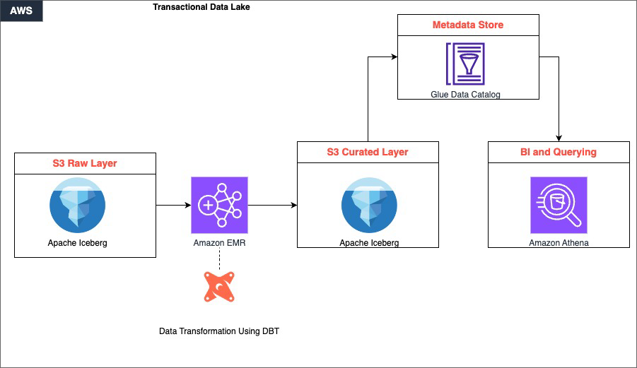
Raw data is ingested and stored in Amazon S3, which serves as the foundational storage layer. This layer supports multiple data formats and enables efficient data partitioning through Apache Iceberg’s table format. This ensures that data is organized and accessible from the moment it lands. Then, Amazon EMR takes over as the distributed computing engine, using Apache Spark to process large-scale datasets in parallel, handling the heavy lifting of reading, transforming, and writing data across the lake.

Sitting within the processing layer, dbt drives the transformation logic. It applies SQL-based, version-controlled transformations that convert raw, unstructured data in the S3 raw layer into clean, curated datasets stored back in S3. This maintains ACID compliance and schema consistency throughout.

Finally, the curated data is available for consumption through Amazon Athena, which provides a serverless, one-time querying capability directly on S3. With this, analysts and business users can run interactive SQL queries without managing any infrastructure. Together, these components form a continuous pipeline: data flows from ingestion through distributed processing and structured transformation, ultimately surfacing as reliable, query-ready insights.

Amazon EMR is a cloud-based big data service that streamlines the deployment and management of open source frameworks like Apache Spark, Hive, and Trino. It provides a managed Apache Hadoop environment that organizations can use to process and analyze vast amounts of data efficiently.

Data Build Tool is an open source tool that data teams can use to transform and model data using SQL. It promotes best practices for data modeling, testing, and documentation, streamlining maintenance and collaboration on data pipelines.

Apache Iceberg is an open table format designed for large-scale analytics on data lakes. It supports features like transactions, time travel, and data partitioning, which are essential for building reliable and performant data lakes. By using Iceberg, organizations can maintain data integrity and enable efficient querying and processing of data.

When combined, these three technologies provide a powerful solution for building transactional data lakes. Amazon EMR provides the scalable and managed infrastructure for running big data workloads, dbt enables efficient data modeling and transformation, and Apache Iceberg provides data consistency and reliability within the data lake.

Prerequisites

Before proceeding with the solution walkthrough, make sure that the following are in place:

  • AWS Account – An active AWS account with sufficient permissions to create and manage EMR clusters, S3 buckets, Athena workgroups, and AWS Glue Data Catalog resources
  • IAM Roles – The following IAM roles must exist and have appropriate permissions:
    • EMR_DefaultRole – Service role for Amazon EMR
    • EMR_EC2_DefaultRole – Amazon Elastic Compute Cloud (Amazon EC2) instance profile for EMR nodes
  • AWS Command Line Interface (AWS CLI) – Installed and configured with credentials for your target AWS account and AWS Region (refer to Step 1.1 for setup instructions)
  • Python 3.8+ – Installed on your local machine or workspace for setting up the dbt virtual environment
  • Pip – Python package manager available for installing dbt and its dependencies
  • Git – Installed on the EMR primary node or local environment for version control and dbt package management
  • Amazon Athena – Athena query editor access with a configured S3 output location for query results
  • AWS Glue Data Catalog – Enabled as the metastore for Amazon EMR and Athena (no additional setup required if using the default AWS Glue integration)
  • S3 Bucket Naming – Prepare a unique identifier to suffix S3 bucket names, ensuring global uniqueness across all three buckets created in Step 1.3
  • Network Access – Make sure that your local machine can reach the Amazon EMR primary node’s DNS over port 10001 (Thrift/HiveServer2) for dbt connectivity; configure security groups accordingly

Solution walkthrough

Step 1: Environment setup

  1. Install the AWS CLI on your workspace by following the instructions in Installing or updating the latest version of the AWS CLI. To configure AWS CLI interaction with AWS, refer to Quick setup.
  2. Create EMR cluster.

    Create the following JSON file with the following contents emr-config.json:

    [
      {
        "Classification": "iceberg-defaults",
        "Properties": {
          "iceberg.enabled": "true"
        }
      },
      {
        "Classification": "spark-hive-site",
        "Properties": {
          "hive.metastore.client.factory.class": "com.amazonaws.glue.catalog.metastore.AWSGlueDataCatalogHiveClientFactory"
        }
      }
    ]

    Run the following command on your AWS CLI, updating the preferred AWS Region:

    aws emr create-cluster \
    --name "Iceberg-DBT-Cluster" \
    --release-label emr-7.7.0 \
    --applications Name=Spark Name=Hive Name=Livy \
    --ec2-attributes InstanceProfile=EMR_EC2_DefaultRole \
    --instance-type c3.4xlarge \
    --instance-count 1 \
    --service-role EMR_DefaultRole \
    --configurations file://emr-config.json \
    --region [region]

  3. Set up S3 buckets.
    Create the following S3 bucket using the AWS CLI after updating the bucket name.

    aws s3 mb s3://amzn-s3-demo-transactional-datalake-raw-[unique-identifier]
    aws s3 mb s3://amzn-s3-demo-transactional-datalake-curated-[unique-identifier]
    aws s3 mb s3://amzn-s3-demo-transactional-datalake-analytics-[unique-identifier]
    

Step 2. Raw layer implementation

The raw layer serves as the foundation of our data lake, ingesting and storing data in its original form. This layer is important for maintaining data lineage and enabling reprocessing if needed. We use Apache Iceberg tables to store our raw data, which provides benefits such as ACID transactions, schema evolution, and time travel capabilities.

In this step, we create a dedicated database for our raw data and set up tables for customers, products, and sales using Amazon Athena. These tables are configured to use the Iceberg table format and are compressed using the ZSTD algorithm to optimize storage. The LOCATION property specifies where the data will be stored in Amazon S3 so that data is organized and accessible.

After creating the tables, we insert sample data to simulate real-world scenarios. We use this data throughout the rest of the implementation to demonstrate the capabilities of our data lake architecture.

Update the respective bucket name in each create table bucket name from the previous step:

  1. Create database and tables
    -- Create Raw Database
    CREATE SCHEMA raw_sales_analytics_data_layer;
    
    -- Create Customers Table
    CREATE TABLE raw_sales_analytics_data_layer.customers (
        CustomerID string,
        CustomerName string,
        Region string,
        inserted_timestamp timestamp
    )
    LOCATION 's3://[bucket_name]/raw_sales_analytics_data_layer/customers'
    TBLPROPERTIES (
        'table_type'='iceberg', 
        'write_compression'='zstd'
    );
    
    -- Create Products Table
    CREATE TABLE raw_sales_analytics_data_layer.products (
        productid string,
        productname string,
        category string,
        supplier string,
        inserted_timestamp timestamp
    )
    LOCATION 's3://[bucket_name]/raw_sales_analytics_data_layer/products'
    TBLPROPERTIES (
        'table_type'='iceberg', 
        'write_compression'='zstd'
    );

  2. Insert sample data
    -- Insert Customers
    INSERT INTO raw_sales_analytics_data_layer.customers
    VALUES 
        ('201', Jane Doe', 'Central', current_timestamp),
        ('202', Arnav Desai, 'North', current_timestamp),
        ('203', Kwaku Mensah, 'West', current_timestamp);
    
    -- Insert Products
    INSERT INTO raw_sales_analytics_data_layer.products
    VALUES
        ('1', 'Laptop', 'Electronics', 'AnyAuthority', current_timestamp),
        ('2', 'Smartphone', 'Electronics', 'AnyCompany', current_timestamp);
    
    -- Insert Sales
    INSERT INTO raw_sales_analytics_data_layer.sales
    VALUES
        ('ORD001', '1', '201', '2025-04-01', 1299.99, current_timestamp),
        ('ORD002', '2', '202', '2025-04-02', 899.99, current_timestamp);

Step 3: dbt setup and configuration

Setting up dbt involves installing the necessary packages, configuring the connection to the data warehouse (in this case, Amazon EMR), and setting up the project structure.

We start by creating a Python virtual environment to isolate our dbt installation. Then, we install dbt-core and the Spark adapter, which allows dbt to connect to the EMR cluster. The profiles.yml file is configured to connect to the EMR cluster using the Thrift protocol, while the dbt_project.yml file defines the overall structure of the dbt project, including model materialization strategies and file formats.

  1. Install prerequisites
    # Create Python virtual environment
    python -m venv dbt-env
    source dbt-env/bin/activate
    
    # Install required packages
    pip install dbt-core dbt-spark[PyHive]
    
    # Install git
    yum install git

  2. Configure dbt profiles
    # ~/.dbt/profiles.yml
    sales_analytics:
      target: dev
      outputs:
        dev:
          type: spark
          method: thrift
          host: your-emr-master-dns
          port: 10001
          schema: curated_sales_analytics_data_layer
          threads: 4

  3. Project configuration
    # dbt_project.yml
    name: 'sales_analytics'
    version: '1.0.0'
    config-version: 2
    
    profile: 'sales_analytics'
    
    model-paths: ["models"]
    analysis-paths: ["analyses"]
    test-paths: ["tests"]
    seed-paths: ["seeds"]
    macro-paths: ["macros"]
    
    target-path: "target"
    clean-targets:
        - "target"
        - "dbt_packages"
    
    models:
      sales_analytics:
        dim:
          +materialized: table
          +file_format: iceberg
        ads:
          +materialized: table
          +file_format: iceberg

Step 4: dbt models implementation

In this step, we implement dbt models, which define the transformations that we will apply to raw data. We start by configuring data sources in the sources.yml file, which allows dbt to reference raw tables easily.

We then create dimension models for customers and products, and a fact model for sales.

These models use incremental materialization strategies to efficiently update data over time. The incremental strategy processes only new or updated records, significantly reducing the time and resources required for each run.

  1. Source configuration
    # models/sources.yml
    version: 2
    sources:
      - name: raw_sales
        database: raw_sales_analytics_data_layer
        schema: raw_sales_analytics_data_layer
        tables:
          - name: customers
            columns:
              - name: CustomerID
                tests:
                  - unique
                  - not_null
          - name: products
          - name: sales

  2. Dimension models
    -- models/dim/dim_customers.sql
    {{ config(
        materialized='incremental',
        unique_key='customerid',
        incremental_strategy='merge'
    ) }}
    
    WITH source_data AS (
        SELECT 
            customerid,
            customername,
            region,
            inserted_timestamp,
            ROW_NUMBER() OVER (
                PARTITION BY customerid 
                ORDER BY inserted_timestamp DESC
            ) as row_number
        FROM {{ source('raw_sales_analytics_data_layer', 'customers') }}
        {% if is_incremental() %}
        WHERE inserted_timestamp > (SELECT MAX(inserted_timestamp) FROM {{ this }})
        {% endif %}
    )
    
    SELECT 
        customerid,
        customername,
        region,
        inserted_timestamp
    FROM source_data
    WHERE row_number = 1

  3. Product models
    -- models/dim/dim_products.sql
    {{ config(
        materialized='incremental',
        unique_key='productid',
        incremental_strategy='merge'
    ) }}
    
    WITH source_data AS (
        SELECT
            productid,
            productname,
            category,
            supplier,
            inserted_timestamp,
            ROW_NUMBER() OVER (
                PARTITION BY productid
                ORDER BY inserted_timestamp DESC
            ) as row_number
        FROM {{ source('raw_sales_analytics_data_layer', 'products') }}
        {% if is_incremental() %}
        WHERE inserted_timestamp > (SELECT MAX(inserted_timestamp) FROM {{ this }})
        {% endif %}
    )
    
    SELECT
        s.productid,
        s.productname,
        s.category,
        s.supplier,
        s.inserted_timestamp
    FROM source_data s
    WHERE s.row_number = 1
    {% if is_incremental() %}
        AND NOT EXISTS (
            SELECT 1
            FROM {{ this }} t
            WHERE t.productid = s.productid
            AND t.inserted_timestamp >= s.inserted_timestamp
        )
    {% endif %}

  4. Fact models
    -- models/dim/fact_sales.sql
    {{ config(
        materialized='incremental',
        unique_key='orderid',
        incremental_strategy='merge'
    ) }}
    
    WITH source_data AS (
        SELECT
            orderid,
            productid,
            customerid,
            date,
            salesamount,
            inserted_timestamp,
            ROW_NUMBER() OVER (
                PARTITION BY orderid
                ORDER BY inserted_timestamp DESC
            ) as row_number
        FROM {{ source('raw_sales_analytics_data_layer', 'sales') }}
        {% if is_incremental() %}
        WHERE orderid NOT IN (SELECT orderid FROM {{ this }})  -- Changed condition
        {% endif %}
    )
    
    SELECT
        s.orderid,
        s.productid,
        s.customerid,
        s.date,
        s.salesamount,
        s.inserted_timestamp
    FROM source_data s
    WHERE s.row_number = 1

Step 5: Analytics layer

The analytics layer builds upon dimension and fact models to create more complex analyzes. In this step, we create a daily sales analysis model that combines data from fact_sales, dim_customers, and dim_products models.

We also implement a customer insights model that analyzes purchase patterns across different Regions and product categories.

These analytics models demonstrate how we can use our transformed data to generate valuable business insights. By materializing these models as Iceberg tables, we make sure that they benefit from the same ACID transactions and time travel capabilities as our raw and transformed data.

  1. Daily sales analysis

    The analytics layer introduces a fact_sales_analysis model that consolidates transactional sales data with customer and product dimensions to enable business-ready reporting. Built as an incremental model with a merge strategy, it efficiently processes data by deduplicating records using the latest inserted timestamp per order, enabling reliable downstream consumption without full table refreshes.

    -- models/ads/fact_sales_analysis.sql
    {{ config(
        materialized='incremental',
        unique_key='orderid',
        incremental_strategy='merge'
    ) }}
    
    WITH source_data AS (
        SELECT
            s.orderid,
            s.date,
            s.salesamount,
            c.customername,
            c.region,
            p.productname,
            p.category,
            p.supplier,
            s.inserted_timestamp,
            ROW_NUMBER() OVER (
                PARTITION BY s.orderid
                ORDER BY s.inserted_timestamp DESC
            ) as row_number
        FROM {{ ref('fact_sales') }} s
        JOIN {{ ref('dim_customers') }} c ON s.customerid = c.customerid
        JOIN {{ ref('dim_products') }} p ON s.productid = p.productid
        {% if is_incremental() %}
        WHERE s.orderid NOT IN (SELECT orderid FROM {{ this }})
        {% endif %}
    )
    
    SELECT
        s.orderid,
            s.date,
            s.salesamount,
            s.customername,
            s.region,
            s.productname,
            s.category,
            s.supplier,
            s.inserted_timestamp
    FROM source_data s
    WHERE s.row_number = 1

  2. Customer insights

    The customer_purchase_patterns model aggregates sales activity across customer Regions and product categories to surface revenue trends and buying behavior. Materialized as an Iceberg table in the analytics schema, it provides a performant and scalable foundation for customer segmentation, Regional performance analysis, and category-level revenue attribution.

    -- models/analytics/customer_purchase_patterns.sql
    {{
        config(
            materialized='table',
            file_format='iceberg',
            schema='analytics'
        )
    }}
    
    SELECT
        dc.Region,
        dp.category,
        COUNT(DISTINCT fs.orderid) as total_orders,
        COUNT(DISTINCT dc.customerid) as unique_customers,
        SUM(fs.salesamount) as total_revenue,
        SUM(fs.salesamount) / COUNT(DISTINCT dc.customerid) as revenue_per_customer
    FROM {{ ref('fact_sales') }} fs
    JOIN {{ ref('dim_customers') }} dc ON fs.customerid = dc.customerid
    JOIN {{ ref('dim_products') }} dp ON fs.productid = dp.productid
    GROUP BY dc.Region, dp.category

Step 6: Transactional operations and time travel with Apache Iceberg

This section demonstrates how to use Apache Iceberg’s time travel capabilities and transactional operations using actual snapshot data from our dim_customers table. We walk through querying data at different points in time and comparing changes between snapshots.

  1. Transactional capabilities

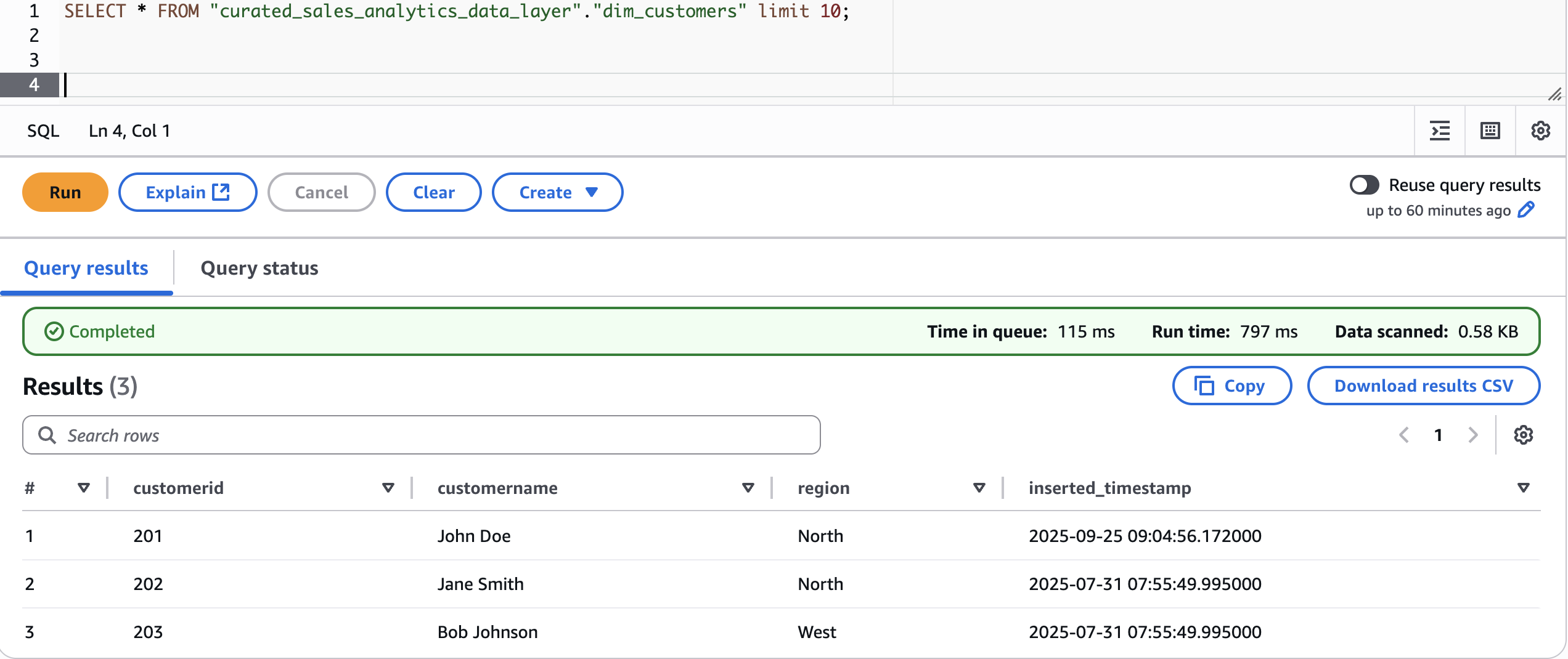
    Let’s first look at current data:

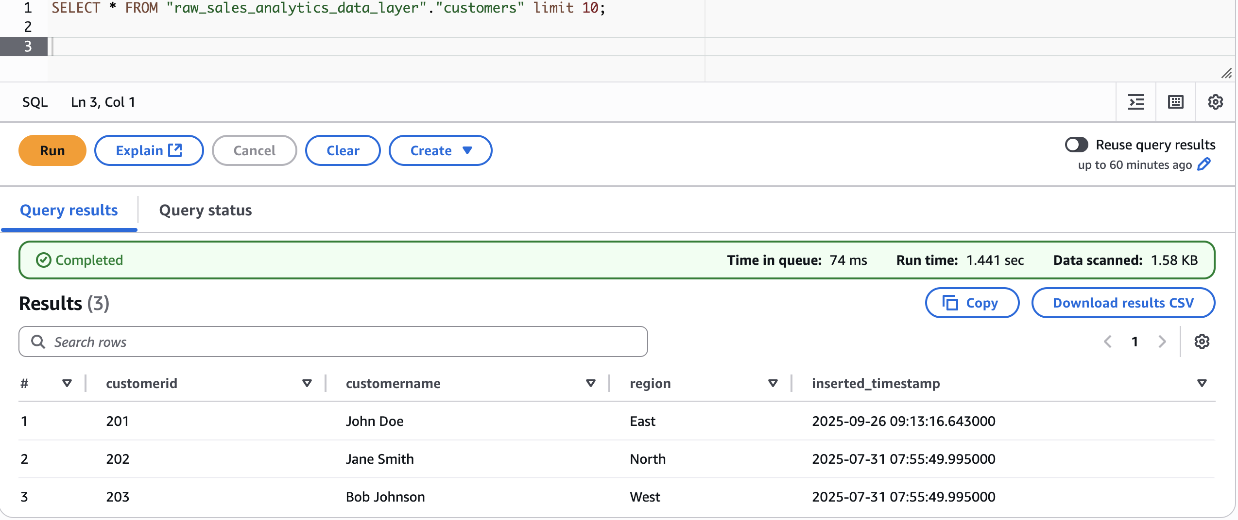
    Now, modify the raw layer data for customerid 201 and change the Region to East

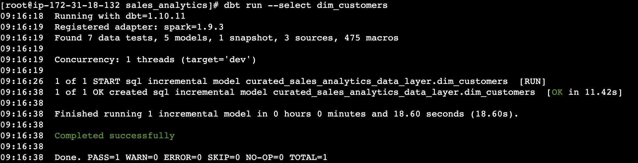
    Run the dbt model for dim_customers to sync the changes

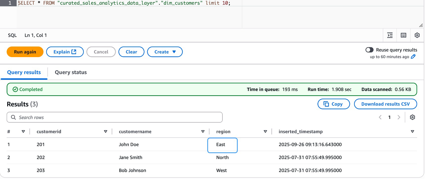
    Validate the data in curated layer for dim_customers dimension table

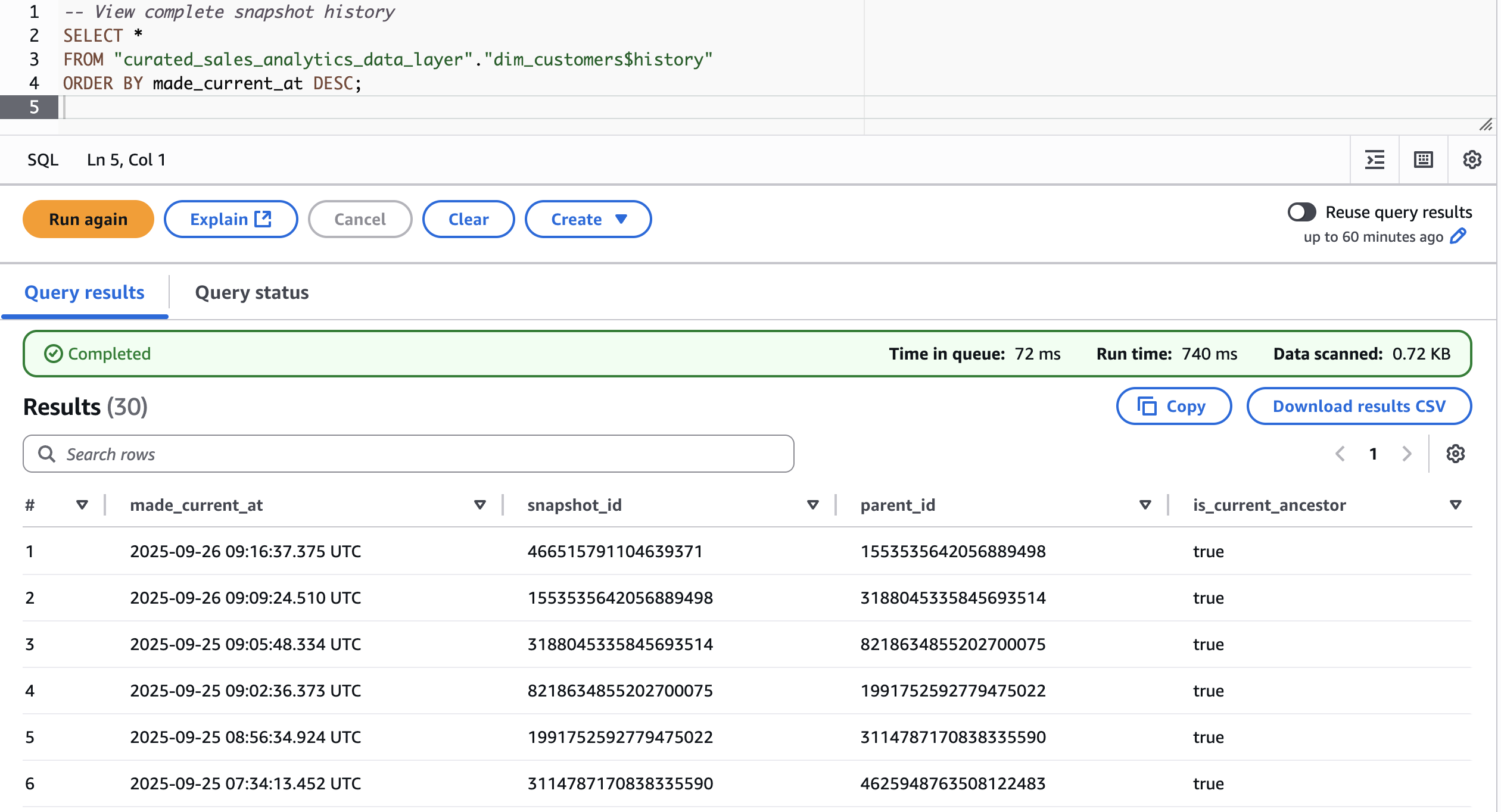
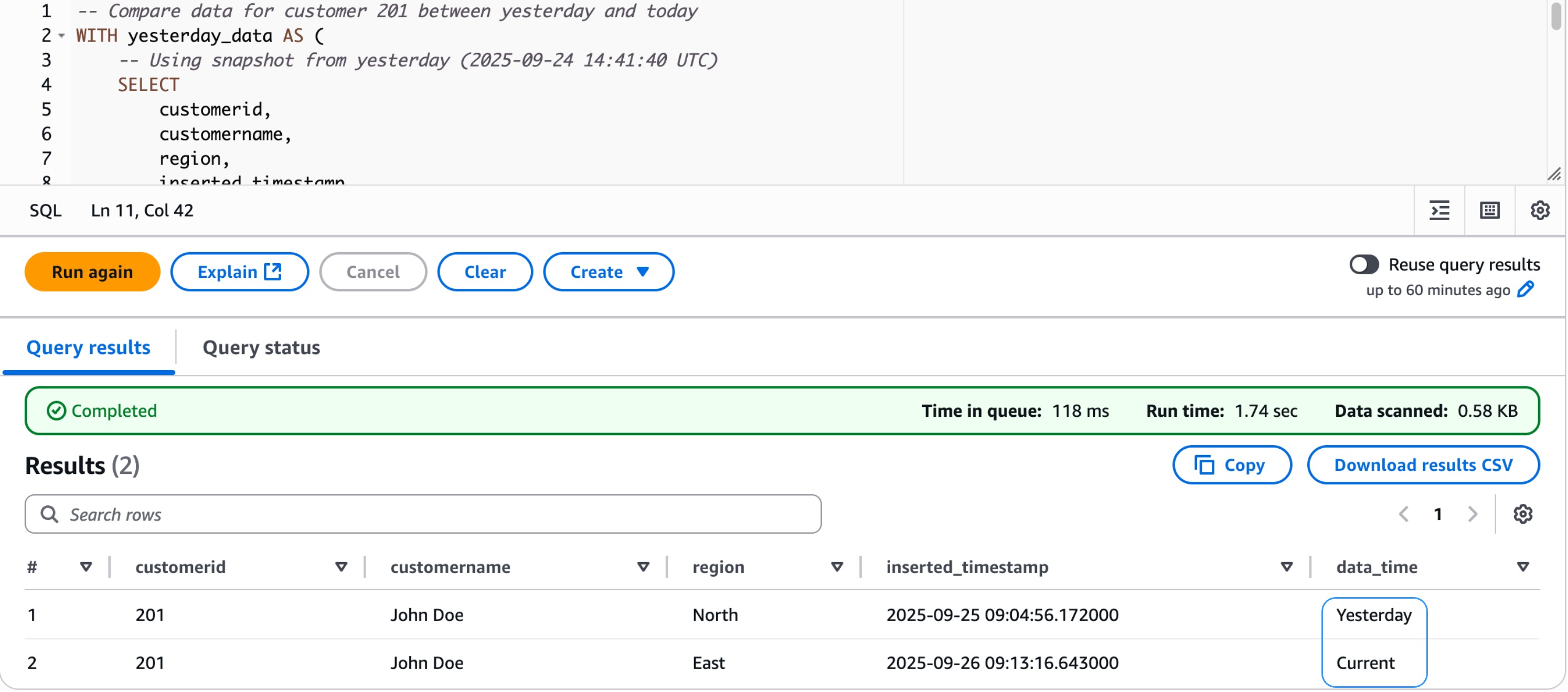
  2. Time-travel capabilities

    First, let’s fetch snapshots for customers dimension table in curated layer

    Now, find the data state before and after the modification.

Step 7: Data quality tests

Data quality is a critical pillar of any reliable data pipeline. In this step, we define and enforce quality checks directly within the dbt project using schema-level test configurations. Rather than relying on one-time validation scripts, with dbt’s built-in testing framework, we can declaratively specify expectations on our models, ensuring that key fields remain unique, non-null, and consistent across the data layer before they reach downstream consumers.

  1. Generic tests configuration

    The schema.yml file serves as the central contract for model integrity. Here, we apply generic tests on the fact_sales and dim_customers models to catch data anomalies early in the pipeline.

    # models/schema.yml
    version: 2
    
    models:
      - name: fact_sales
        columns:
          - name: orderid
            tests:
              - unique
              - not_null
          - name: salesamount
            tests:
              - not_null
    
      - name: dim_customers
        columns:
          - name: customerid
            tests:
              - unique
              - not_null

Step 8: Maintenance procedures

A well-functioning data pipeline requires ongoing maintenance to remain performant and auditable over time. This step covers two essential practices, table optimization to keep data storage efficient, and snapshot management to track historical changes in source data. Together, these procedures keep the pipeline reliable, cost-effective, and capable of supporting time-based analysis.

  1. Table optimization

    As data accumulates in Delta or Iceberg tables, small files and fragmented storage can degrade query performance. The optimize_table macro provides a reusable utility to run Databricks’ OPTIMIZE command on any target table, consolidating small files and improving read efficiency without manual intervention.

    -- macros/optimize_table.sql
    {% macro optimize_table(table_name) %}
        {% set query %}
            OPTIMIZE {{ table_name }}
        {% endset %}
        {% do run_query(query) %}
    {% endmacro %}

  2. Snapshot management

    To maintain a historical record of customer data changes, we use dbt snapshots with a timestamp-based strategy. The customers_snapshot model captures row-level changes from the raw source layer and persists them in a dedicated snapshots schema, enabling point-in-time analysis and audit trails.

    -- snapshots/customer_snapshot.sql
    {% snapshot customers_snapshot %}
    {{
        config(
          target_schema='snapshots',
          unique_key='CustomerID',
          strategy='timestamp',
          updated_at='inserted_timestamp'
        )
    }}
    
    SELECT * FROM {{ source('raw_sales_analytics_data_layer', 'customers') }}
    
    {% endsnapshot %}

Step 9: Monitoring and logging

Observability is an essential aspect of any production-grade data pipeline. This step establishes logging and monitoring practices within the dbt project to track pipeline runs, capture errors, and support debugging. With structured logging enabled, teams gain visibility into model execution, test results, and runtime behavior, streamlining issue diagnosis and maintaining operational confidence.

  1. dbt logging configuration

    The dbt_project.yml logging configuration directs dbt to write logs to a dedicated path and outputs them in JSON format. JSON-structured logs are particularly useful for integration with log aggregation tools and monitoring dashboards, enabling automated alerting and audit trail management.

    # dbt_project.yml
    logs:
      path: logs
      enable_json: true

Step 10. Deployment and running

With the pipeline fully built, tested, and maintained, the final step covers how to deploy and execute dbt models across different scenarios. Whether running a complete refresh, processing incremental updates, or validating data quality, these commands form the operational backbone of day-to-day pipeline management.

  1. Full refresh

    A full refresh rebuilds all models from scratch, reprocessing the entire dataset. This is typically used after significant schema changes, backfills, or when incremental state needs to be reset.

    dbt run --full-refresh

  2. Incremental update

    For routine pipeline runs, incremental updates process only new or changed data, significantly reducing compute time and cost. The following command targets specific models (dim_customers and fact_sales) allowing selective execution without triggering the full DAG.

    dbt run --select dim_customers fact_sales

  3. Testing

    After models are run, data quality tests defined in the schema configuration are executed to validate integrity across all models. This validates that constraints such as uniqueness and non-null checks are met before data reaches downstream consumers.

    dbt test

Step 11. Cleanup

  1. Infrastructure cleanup
    # Delete EMR cluster
    aws emr terminate-clusters --cluster-id <cluster-id>
    
    # Remove S3 buckets
    aws s3 rb s3://amzn-s3-demo-transactional-datalake-raw-bucket-[unique-identifier] --force
    aws s3 rb s3://amzn-s3-demo-transactional-datalake-curated-bucket-[unique-identifier] --force
    aws s3 rb s3://amzn-s3-demo-transactional-datalake-analytics-bucket-[unique-identifier] --force

  2. Database cleanup
    DROP SCHEMA raw_sales_analytics_data_layer CASCADE;
    DROP SCHEMA curated_sales_analytics_data_layer CASCADE;

Conclusion

In this post, you learned how to build a transactional data lake on Amazon EMR using dbt and Apache Iceberg, from environment setup and modeling raw data, to quality enforcing, snapshot management, and incremental pipeline deployment. The architecture brings together the scalability of Amazon EMR, dbt’s transformation capabilities, and Iceberg’s ACID-compliant table format to deliver a reliable, maintainable, and cost-efficient data platform.

To get started, see the Amazon EMR documentation to deploy this architecture in your own environment. Whether you’re modernizing a legacy data platform or building a new analytics foundation, this stack gives you the flexibility to scale with confidence.

About the authors

Umesh Pathak

Umesh Pathak

Umesh is a Data Analytics Lead Consultant at AWS ProServe, based in India. When not solving complex data challenges, Umesh is out on the trails — an avid runner and hiker who brings the same discipline and drive to fitness as he does to his work.

Amol Guldagad

Amol Guldagad

Amol is a Data Analytics Lead Consultant based in India. He helps customers to accelerate their journey to the cloud and innovate using AWS analytics services.

Building scalable AWS Lake Formation governed data lakes with dbt and Amazon Managed Workflows for Apache Airflow

Post Syndicated from Abhilasha Agarwal original https://aws.amazon.com/blogs/big-data/building-scalable-aws-lake-formation-governed-data-lakes-with-dbt-and-amazon-managed-workflows-for-apache-airflow/

Organizations often struggle with building scalable and maintainable data lakes—especially when handling complex data transformations, enforcing data quality, and monitoring compliance with established governance. Traditional approaches typically involve custom scripts and disparate tools, which can increase operational overhead and complicate access control. A scalable, integrated approach is needed to simplify these processes, improve data reliability, and support enterprise-grade governance.

Apache Airflow has emerged as a powerful solution for orchestrating complex data pipelines in the cloud. Amazon Managed Workflows for Apache Airflow (MWAA) extends this capability by providing a fully managed service that eliminates infrastructure management overhead. This service enables teams to focus on building and scaling their data workflows while AWS handles the underlying infrastructure, security, and maintenance requirements.

dbt enhances data transformation workflows by bringing software engineering best practices to analytics. It enables analytics engineers to transform warehouse data using familiar SQL select statements while providing essential features like version control, testing, and documentation. As part of the ELT (Extract, Load, Transform) process, dbt handles the transformation phase, working directly within a data warehouse to enable efficient and reliable data processing. This approach allows teams to maintain a single source of truth for metrics and business definitions while enabling data quality through built-in testing capabilities.

In this post, we show how to build a governed data lake that uses modern data tools and AWS services.

Solution overview

We explore a comprehensive solution that includes:

  • A metadata-driven framework in MWAA that dynamically generates directed acyclic graphs (DAGs), significantly improving pipeline scalability and reducing maintenance overhead.
  • dbt with Amazon Athena adapter to implement modular, SQL-based data transformations directly on a data lake, enabling well-structured, and thoroughly tested transformations.
  • An automated framework that proactively identifies and segregates problematic records, maintaining the integrity of data assets.
  • AWS Lake Formation to implement fine-grained access controls for Athena tables, ensuring proper data governance and security throughout a data lake environment.

Together, these components create a robust, maintainable, and secure data management solution suitable for enterprise-scale deployments.

The following architecture illustrates the components of the solution.

The workflow contains the following steps:

  1. Multiple data sources (PostgreSQL, MySQL, SFTP) push data to an Amazon S3 raw bucket
  2. S3 event triggers AWS Lambda Function
  3. Lambda function triggers the MWAA DAG to convert file formats to parquet
  4. Data is stored in Amazon S3 formatted bucket under formatted_stg prefix
  5. Crawler crawls the data in formatted_stg prefix in the formatted bucket and creates catalog tables
  6. dbt using Athena adapter processes the data and puts the processed data after data quality checks under formatted prefix in Formatted bucket
  7. dbt using Athena adapter can perform further transformations on the formatted data and put the transformed data in Published bucket

Prerequisites

To implement this solution, the following prerequisites need to be met.

Deploy the solution

For this solution, we provide an AWS CloudFormation (CFN) template that sets up the services included in the architecture, to enable repeatable deployments.

Note:

  • US-EAST-1 Region is required for the deployment.
  • Deploying this solution will involve costs associated with AWS services.

To deploy the solution, complete the following steps:

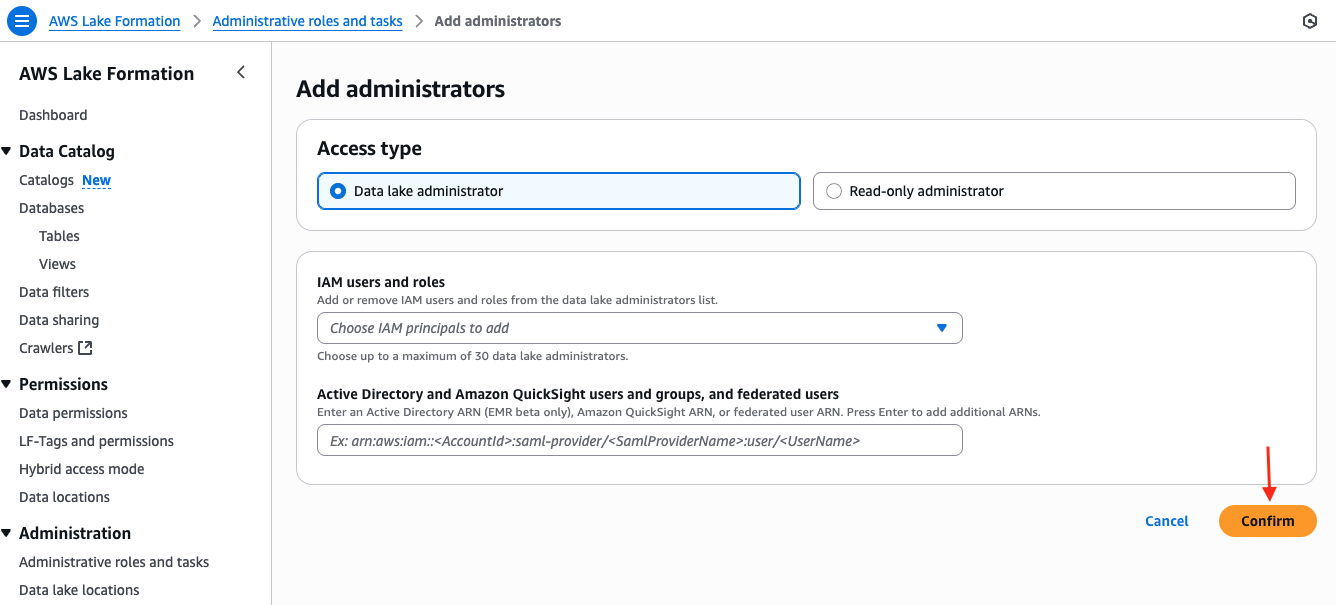
  1. Before deploying the stack, open the AWS Lake Formation console. Add your console role as a Data Lake Administrator and choose Confirm to save the changes.
  2. Download the CloudFormation template.
    After the file is downloaded to the local machine, follow the steps below to deploy the stack using this template:

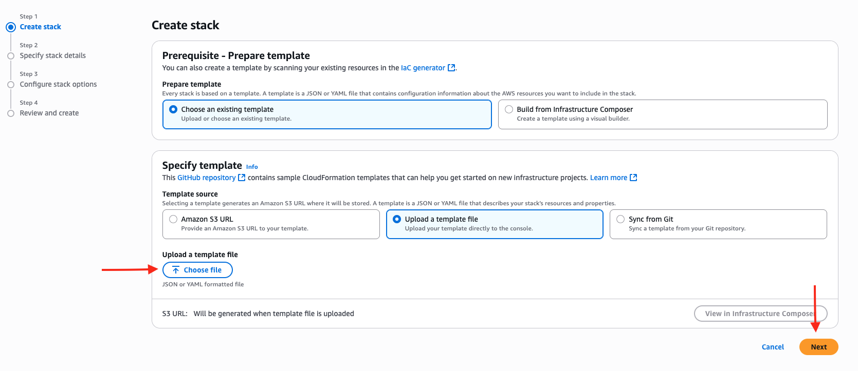
    1. Open the AWS CloudFormation Console.
    2. Choose Create stack and choose With new resources (standard).
    3. Under Specify template, select Upload a template file.
    4. Select Choose file and upload the CFN template that was downloaded earlier.
    5. Choose Next to proceed.

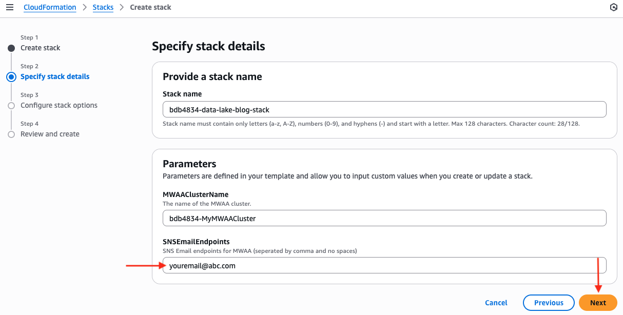
  3. Enter a stack name (for example, bdb4834-data-lake-blog-stack) and configure the parameters (bdb4834-MWAAClusterName can be left as the default value and update SNSEmailEndpoints with your email address), then choose Next.
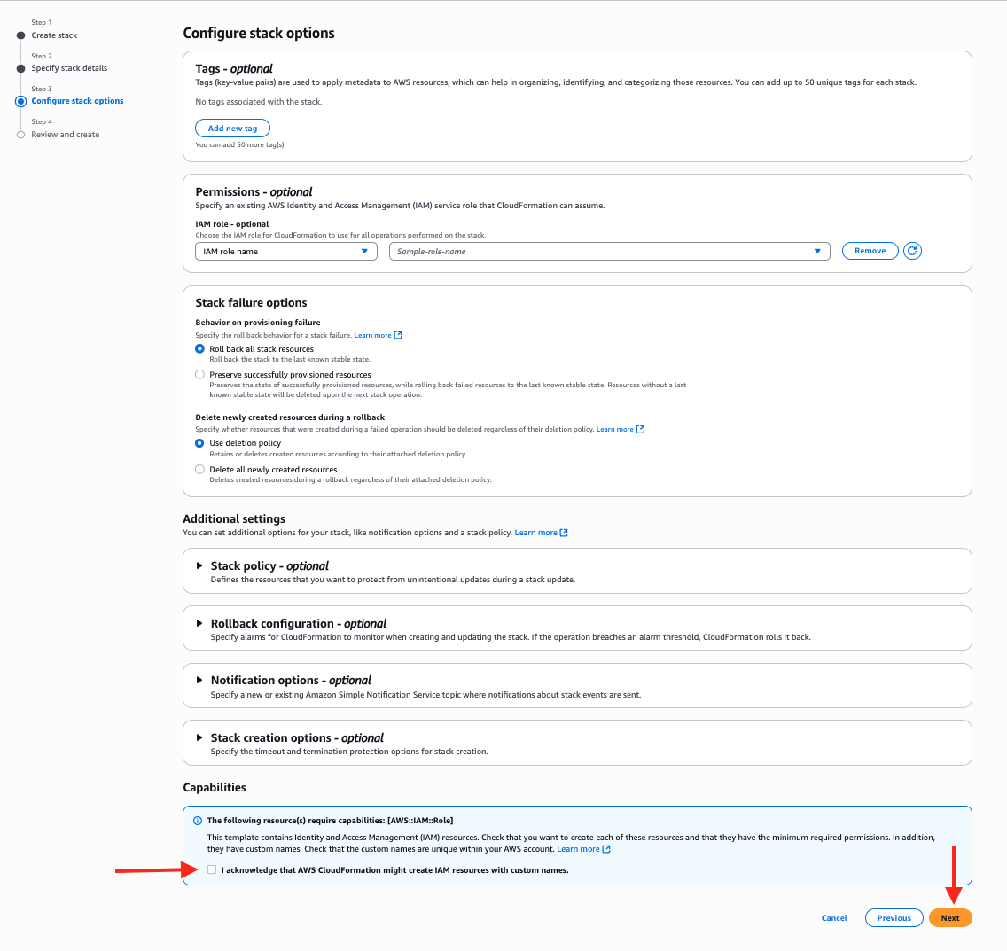
  4. Select “I acknowledge that AWS CloudFormation might create IAM resources with custom names” and choose Next

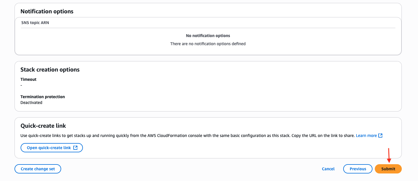
  5. Review all the configuration details on the next page, then choose Submit.
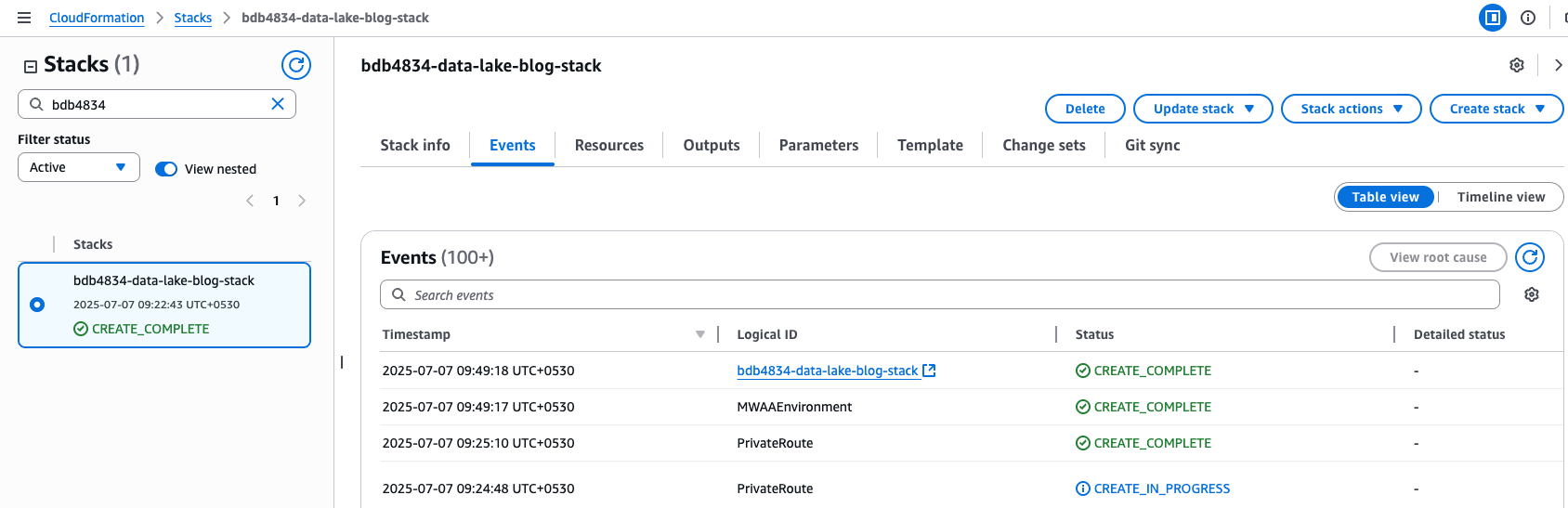
  6. Wait for the stack creation to complete in the AWS CloudFormation console. The process typically takes approximately 35 to 40 minutes to provision all required resources.

    The following table shows resources available in the AWS Account after CloudFormation template deployment is successfully completed:

    Resource Type Description Example Resource Name
    S3 Buckets For storing raw, processed data and assets bdb4834-mwaa-bucket-<AWS_ACCOUNT>-<AWS_REGION>,bdb4834-raw-bucket-<AWS_ACCOUNT>-<AWS_REGION>,bdb4834-formatted-bucket-<AWS_ACCOUNT>-<AWS_REGION>,bdb4834-published-bucket-<AWS_ACCOUNT>-<AWS_REGION>
    IAM Role Role assumed by MWAA for permissions bdb4834-mwaa-role
    MWAA Environment Managed Airflow environment for orchestration bdb4834-MyMWAACluster
    VPC Network setup required by MWAA bdb4834-MyVPC
    Glue Catalog Databases Logical grouping of metadata for tables bdb4834_formatted_stg,bdb4834_formatted_exception, bdb4834_formatted, bdb4834_published
    Glue Crawlers Automatically catalog metadata from S3 bdb4834-formatted-stg-crawler
    Lambda Lambda to Trigger MWAA DAG on file arrival and to setup Lake Formation Permissions bdb4834_mwaa_trigger_process_s3_files,bdb4834-lf-tags-automation
    Lake Formation Setup Centralized governance and permissions LF-Setup for the above Resources
    Airflow DAGs Airflow DAGs are stored in the S3 bucket named mwaa-bucket-<AWS_ACCOUNT>-<AWS_REGION> under the dags/ prefix. These DAGs are responsible for triggering data pipelines based on either file arrival events or scheduled intervals. The exact functionality of each DAG is explained in the following sections. blog-test-data-processingcrawler-daily-runcreate-audit-tableprocess_raw_to_formatted_stage
  7. When the stack is complete perform the below steps:
    1. Open the Amazon Managed Workflows for Apache Airflow (MWAA) console, choose on Open Airflow UI
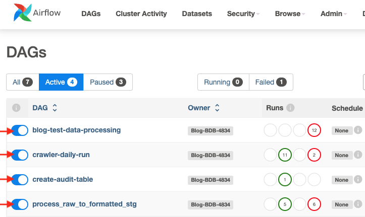
    2. In the DAGs console, locate the following DAGs and unpause them by unchecking the toggle switch (radio button) next to each DAG.

Add sample data to raw S3 bucket and create catalog tables

In this section, we upload sample data to raw S3 bucket (bucket name starting with bdb4834-raw-bucket) and convert the file formats to parquet and run AWS Glue crawler to create catalog tables that are used by dbt in the ELT Process. Glue Crawler automatically scans the data in S3 and creates or updates tables in the Glue Data Catalog, making the data queryable and accessible for transformation.

  1. Download the sample data.
  2. Zip folder contains two sample data files, cards.json and customers.json
    Schema for cards.json

    Field Data Type Description
    cust_id String Unique customer identifier
    cc_number String Credit card number
    cc_expiry_date String Credit card expiry date

    Schema for customers.json

    Field Data Type Description
    cust_id String Unique customer identifier
    fname String First name
    lname String Last name
    gender String Gender
    address String Full address
    dob String Date of birth (YYYY/MM/DD)
    phone String Phone number
    email String Email address
  3. Open S3 console, choose General purpose buckets in the navigation pane.
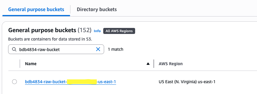
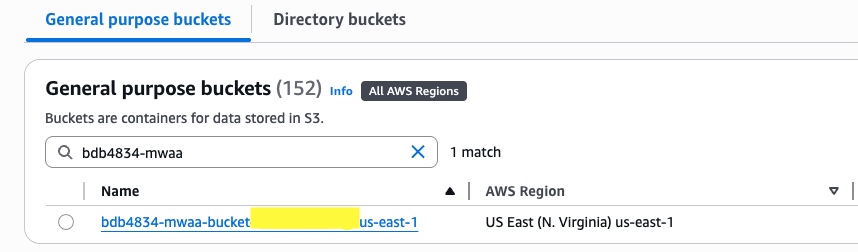
  4. Locate the S3 bucket with a name starting with bdb4834-raw-bucket. This bucket is created by the CloudFormation stack and can also be found under the stack’s Resources tab in the CloudFormation console.
  5. Choose the bucket name to open it, and follow these steps to create the required prefix:
    1. Choose Create folder.
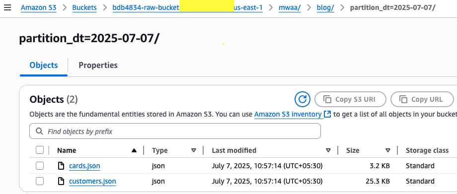
    2. Enter the folder name as mwaa/blog/partition_dt=YYYY-MM-DD/, replacing YYYY-MM-DD with the actual date to be used for the partition.
    3. Choose Create folder to confirm.
  6. Upload the sample data files from the location to the s3 raw bucket prefix.
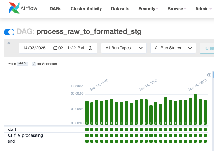
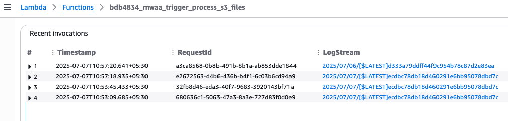
  7. As soon as the files are uploaded, the on_put object event on the raw bucket invokes thebdb4834_mwaa_trigger_process_s3_files lambda which triggers the process_raw_to_formatted_stg MWAA DAG.
    1. In the Airflow UI, choose the process_raw_to_formatted_stg DAG to view execution status. This DAG converts the file formats to parquet and typically completes within a few seconds.
    2. (Optional) To check the Lambda execution details:
      1. On the AWS Lambda Console, choose Functions in the navigation pane.
      2. Select the function named bdb4834_mwaa_trigger_process_s3_files.
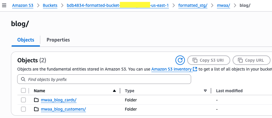
  8. Validate the parquet files are created in formatted bucket (bucket name starting with bdb4834-formatted) under the respective data object prefix.
  9. Before proceeding further, re-upload the Lake Formation metadata file in MWAA bucket.
    1. Open the S3 console, choose General purpose buckets in the navigation pane.
    2. Search for the bucket starting with bdb4834-mwaa-bucket
    3. Choose the bucket name and go to the lakeformation prefix. Download the file named lf_tags_metadata.json. Now, re-upload the same file to the same location.
      Note: This re-upload is necessary because the Lambda function is configured to trigger on file arrival. When the resources were initially created by the CloudFormation stack, the files were simply moved to S3 and did not trigger the Lambda. Re-uploading the file ensures the Lambda function is executed as intended.
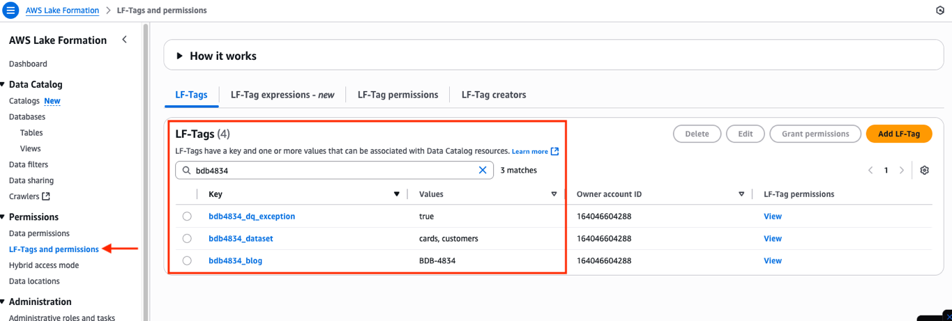
    4. As soon as the file is uploaded, the on_put object event on the MWAA bucket invokes the lf_tags_automation lambda, which creates the Lake Formation (LF) tags as defined in the metadata file and grants access to the specified AWS Identity and Access Management (IAM) roles for read/write.
    5. Validate that the LF-Tags have been created by visiting the Lake Formation Console. In the left navigation pane, choose Permissions, and then select LF-Tags and permissions.
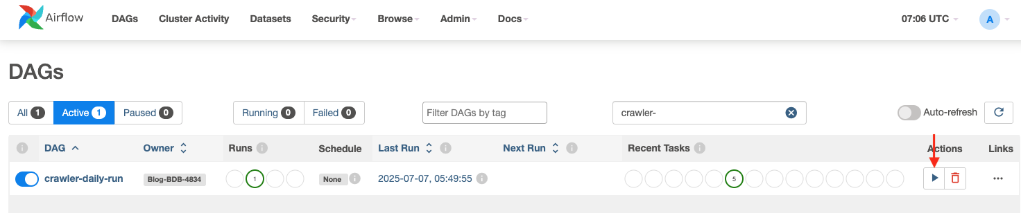
  10. Now, run the crawler DAG to create/update the catalog tables: crawler-daily-run
    1. In the Airflow UI select the crawler-daily-run DAG and choose Trigger DAG to execute it.
    2. This DAG is configured to trigger Glue Crawler which crawls the formatted_stg prefix under the bdb4834-formatted s3 bucket to create catalog tables as per the prefixes available under the formatted_stg prefix.
      bdb4834-formatted-bucket-<aws-account-id>-<region>/formatted_stg/
      

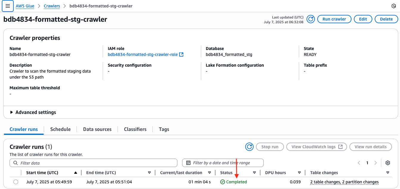
    3. Monitor the execution of the crawler-daily-run DAG until it completes, which typically takes 2 to 3 minutes. The crawler run status can be verified in the AWS Glue Console by following these steps:
      1. Open the AWS Glue Console.
      2. In the left navigation pane, choose Crawlers.
      3. Search for the crawler named bdb4834-formatted-stg-crawler.
      4. Check the Last run status column to confirm the crawler executed successfully.
      5. Choose the crawler name to view additional run details and logs if needed.

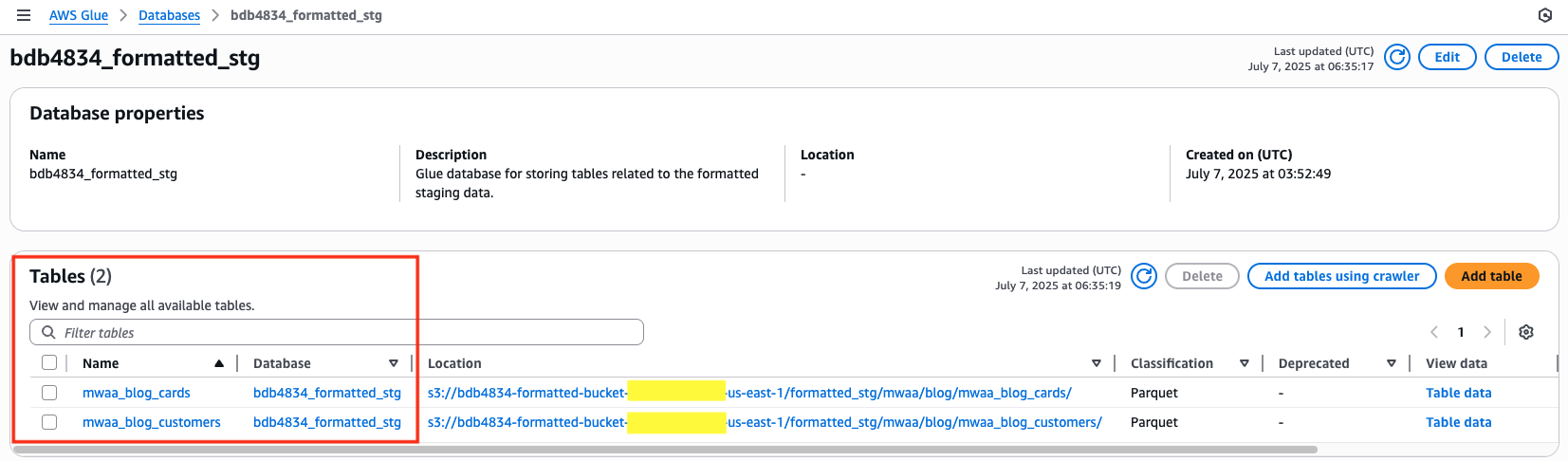
    4. Once the crawler has completed successfully, in the left-hand panel, choose Databases and select the bdb4834_formatted_stg database to view the created tables, which should appear as showing in the following image. Optionally, select the table’s name to view its schema, and then select Table data to open Athena for data analysis. (An error may appear when querying data using Athena due to Lake Formation permissions. Review the Governance using Lake Formation section in this post to resolve the issue.)

Note: If this is the first time Athena is being used, a query result location must be configured by specifying an S3 bucket. Follow the instructions in the AWS Athena documentation to set up the S3 staging bucket for storing query results.

Run model through DAG in MWAA

In this section, we cover how dbt models run in MWAA using Athena adapter to create Glue-catalogued tables and how auditing is done for each run.

  1. After creating the tables in the Glue database using the AWS Glue Crawler in the previous steps, we can now proceed to run the dbt models in MWAA. These models are stored in S3 in the form of SQL files, located at the S3 prefix: bdb4834-mwaa-bucket-<account_id>-us-east-1/dags/dbt/models/
    The following are the dbt models and their functionality:

    • mwaa_blog_cards_exception.sql This model reads data from the mwaa_blog_cards table in the bdb4834_formatted_stg database and writes records with data quality issues to the mwaa_blog_cards_exception table in the bdb4834_formatted_exception database.
    • mwaa_blog_customers_exception.sql This model reads data from the mwaa_blog_customers table in the bdb4834_formatted_stg database and writes records with data quality issues to the mwaa_blog_customers_exception table in the bdb4834_formatted_exception database.
    • mwaa_blog_cards.sql This model reads data from the mwaa_blog_cards table in the bdb4834_formatted_stg database and loads it into the mwaa_blog_cards table in the bdb4834_formatted database. If the target table does not exist, dbt automatically creates it.
    • mwaa_blog_customers.sql This model reads data from the mwaa_blog_customers table in the bdb4834_formatted_stg database and loads it into the mwaa_blog_customers table in the bdb4834_formatted database. If the target table does not exist, dbt automatically creates it.
  2. The mwaa_blog_cards.sql model processes credit card data and depends on the mwaa_blog_customers.sql model to complete successfully before it runs. This dependency is necessary because certain data quality checks—such as referential integrity validations between customer and card records—must be performed beforehand.
    • These relationships and checks are defined in the schema.yml file located in the same S3 path: bdb4834-mwaa-bucket-<account_id>-us-east-1/dags/dbt/models/. The schema.yml file provides metadata for dbt models, including model dependencies, column definitions, and data quality tests. It utilizes macros like get_dq_macro.sql and dq_referentialcheck.sql (found under the macros/ directory) to enforce these validations.

    As a result, dbt automatically generates a lineage graph based on the declared dependencies. This visual graph helps orchestrate model execution order—ensuring models like mwaa_blog_customers.sql run before dependent models such as mwaa_blog_cards.sql, and identifies which models can execute in parallel to optimize the pipeline.

  3. As a pre-step before running models, choose the trigger DAG button for create-audit-table to create audit table for storing run details for each model.
  4. Trigger the blog-test-data-processing DAG in the Airflow UI to start the Model run.
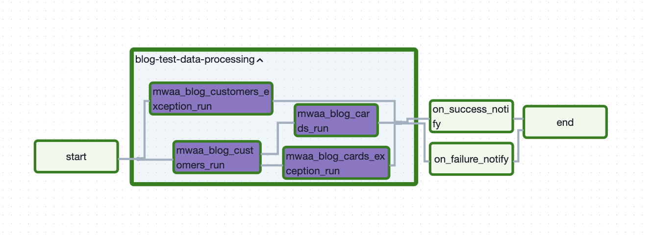
  5. Choose blog-test-data-processing to see the execution status. This DAG runs the models in order and creates Glue catalogued iceberg tables. The flow diagram of a DAG from Airflow UI can be found by choosing Graph after choosing DAG.

    1. The exception models puts the failed records under exception prefix in S3:
      bdb4834-formatted-bucket-<aws-account-id>-<region>/formatted_exception/

      Records that failed are found in an added column, tests_failed, where all the data quality checks that failed for that particular row are added, separated by a pipe (‘|’). (For the mwaa_blog_customers_exception two exception records are found in the table.)

    2. The passed records are put under formatted prefix in S3.
      bdb4834-formatted-bucket-<aws-account-id>-<region>/formatted/

    3. For each run, a run audit is captured in the audit table with execution details like model_nm, process_nm, execution_start_date, execution_end_date, execution_status, execution_failure_reason, rows_affected.
      Find the data in S3 under the prefix bdb4834-formatted-bucket-<aws-account-id>-<region>/audit_control/
    4. Monitor the execution until the DAG completes, which can take up to 2-3 mins. The execution status of the DAG can be seen in the left panel after opening the DAG.
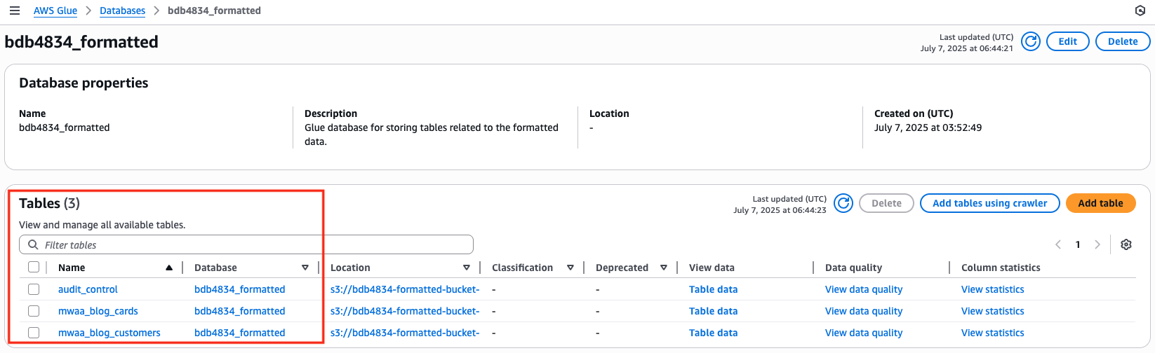
    5. Once the DAG has completed successfully, open the AWS Glue console and select Databases. Select the bdb4834_formatted database, which should create three tables, as shown in the following image.
      Optionally, choose Table data to access Athena for data analysis.
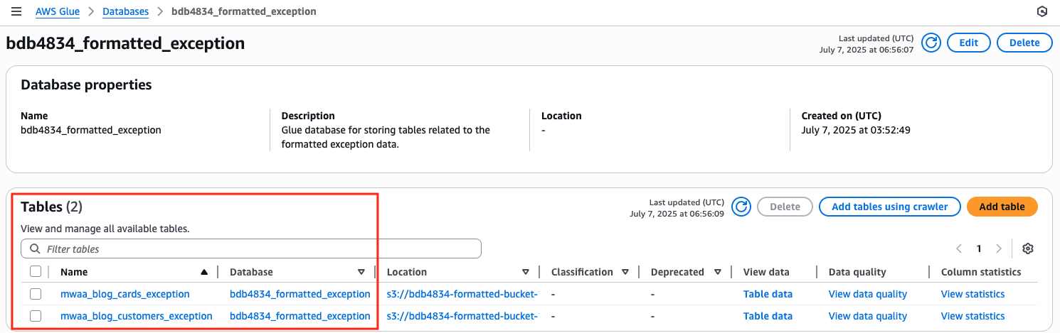
    6. Choose bdb4834_formatted_exception database from under Databases in AWS Glue console, which should create two tables as shown in the following image.
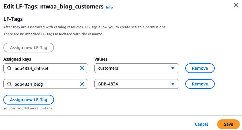
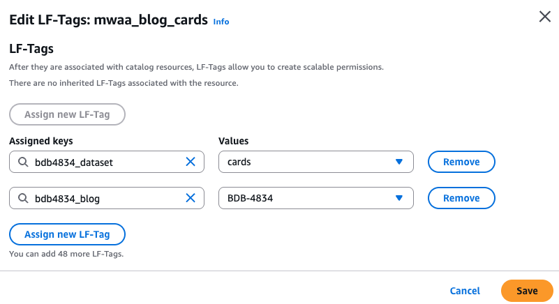
    7. Each model is assigned LF tags through the config block of model itself. Therefore, when the iceberg tables are created through dbt, LF tags are attached to the tables after the run completes.

      Validate the LF tags attached to the tables by visiting the AWS Lake Formation console. In the left navigation pane, choose Tables and look for mwaa_blog_customers or mwaa_blog_cards table under bdb4834_formatted database. Select any table among the two and under Actions, choose Edit LF tags and the tags are attached, as shown in the following screen shot.

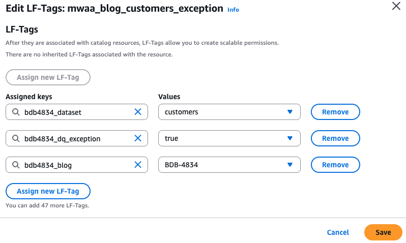
    8. Similarly, for the bdb4834_formatted_exception database, select any one of the exception tables under the bdb4834_formatted_exception database and the LF tags are attached.
    9. Run SQL queries on the tables created by opening the Athena console and running Analytical queries on the tables created above.Sample SQL queries:
      SELECT * FROM bdb4834_formatted.mwaa_blog_cards;
      Output: Total 30 rows

      SELECT * FROM bdb4834_formatted_exception.mwaa_blog_customers_exception;
      Output: Total 2 records

Governance using Lake Formation

In this section, we show how assigning Lake Formation permissions and creating LF tags is automated using the metadata file.Below is a metadata file structure, which is needed for reference when uploading the metadata file for Lake Formation in Airflow S3 bucket, inside the Lake Formation prefix.

Metadata file structure-
{
    "role_arn": "<<IAM_ROLE_ARN>>",
    "access_type": "GRANT",
    "lf_tags": [
      {
        "TagKey": "<<LF_tag_key>>",
        "TagValues": ["<<LF_tag_values>>"]
      }
    ],
	  "named_data_catalog": [
      {
        "Database": "<<Database_Name>>",
        "Table": ""<<Table_Name>>"
      }
    ],
    "table_permissions": ["SELECT", "DESCRIBE"]
  }

Components of the metadata file

  • role_arn: The IAM role that the Lambda function assumes to perform operations.
  • access_type: Specifies whether the action is to grant or revoke permissions (GRANT, REVOKE).
  • lf_tags: Tags used for tag-based access control (TBAC) in Lake Formation.
  • named_data_catalog: A list of databases and tables on which Lake Formation permissions or tags are applied to.
  • table_permissions: Lake Formation-specific permissions (e.g., SELECT, DESCRIBE, ALTER, etc.).

Lambda function bdb4834-lf-tags-automation parses this JSON and grants the required LF tags to the role with given table permissions.

  1. To update the metadata file, download it from the MWAA bucket (lakeformation prefix)
    bdb4834-mwaa-bucket-<<ACCOUNT_NO>>-<<REGION>>/lakeformation/lf_tags_metadata.json

  2. Add a JSON object with the metadata structure defined above, mentioning the IAM role ARN and the tags and tables to which access needs to be granted.
    Example:Let’s assume below is how the metadata file initially looks like:

    
    	[
    	{
        "role_arn": "arn:aws:iam::XXX:role/aws-reserved/sso.amazonaws.com/XX ",
        "access_type": "GRANT",
        "lf_tags": [
          {
            "TagKey": " blog",
            "TagValues": ["bdb-4834"]
          }
        ],
        "named_data_catalog": [],
        "table_permissions": ["SELECT", "DESCRIBE"]
      }
    ]

    Below is the json object that has to be added in the above metadata file:

    
    {
              "role_arn": "arn:aws:iam::XXX:role/aws-reserved/sso.amazonaws.com/XX ",
              "access_type": "GRANT",
              "lf_tags": [],
              "named_data_catalog": [
              {
                "Database": " bdb4834_formatted",
                "Table": "audit_control"
              },
              {
                "Database": " bdb4834_formatted_stg",
                "Table": "*"
              }
             ],
             "table_permissions": ["SELECT", "DESCRIBE"]}


    So now, the final metadata file should look like:

    
    [
      {
        "role_arn": "arn:aws:iam::XXX:role/aws-reserved/sso.amazonaws.com/XX ",
        "access_type": "GRANT",
        "lf_tags": [
          {
            "TagKey": "blog",
            "TagValues": ["bdb-4834"]
          }
        ],
        "named_data_catalog": [],
        "table_permissions": ["SELECT", "DESCRIBE"]
      },
      {
        "role_arn": "arn:aws:iam::XXX:role/aws-reserved/sso.amazonaws.com/XX ",
        "access_type": "GRANT",
        "lf_tags": [],
        "named_data_catalog": [
          {
            "Database": " bdb4834_formatted",
            "Table": "audit_control"
          },
          {
            "Database": " bdb4834_formatted_stg",
            "Table": "*"
          }
        ],
        "table_permissions": ["SELECT", "DESCRIBE"]
      }
    ]

  3. Upon uploading this file at the same location (bdb4834-mwaa-bucket-<<ACCOUNT_NO>>-<<REGION>>/lakeformation/) in S3, the lf_tags_automation lambda is triggered to create LF tags if they don’t exist and then it assigns those tags to the IAM role ARN and also grants permission to the IAM role ARN using named_data_catalog as defined.

    To verify the permissions, go to the Lake Formation console and choose Tables under Data Catalog and search for the table name.

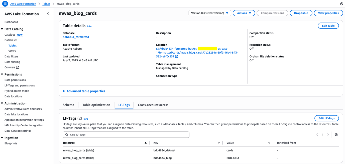
To check LF-Tags, choose the table name and under the LF tags section, all the tags are found attached to this table.

This metadata file used as a structured input to an AWS Lambda function automates the following to perform automated, consistent, and scalable data access governance across the AWS Lake Formation environments:

  • Granting AWS Lake Formation (LF) permissions on Glue Data Catalog resources (like databases and tables).
  • Creating Lake Formation Tags and Applying Lake Formation tags (LF-Tags) for tag-based access control (TBAC).

Explore more on dbt

Now that the deployment includes a bdb4834-published S3 bucket and a published Catalog database, robust dbt models can be built for data transformation and curation.

Here’s how to implement a complete dbt workflow:

  • Start by developing models that follow this pattern:
    • Read from the formatted tables in the staging area
    • Apply business logic, joins, and aggregations
    • Write clean, analysis-ready data to the published schema
  • Tagging for automation: Use consistent dbt tags to enable automatic DAG generation. These tags trigger MWAA orchestration to automatically include new models in the execution pipeline.
  • Adding new models: When working with new datasets, refer to existing models for guidance. Apply appropriate LF tags for data access control. The new LF tags can also now be used for permissions.
  • Enable DAG execution: For new datasets, update the MWAA metadata file to include a new JSON entry. This step is necessary to generate a DAG that executes the new dbt models.

This approach ensures the dbt implementation scales systematically while maintaining automated orchestration and proper data governance.

Clean up

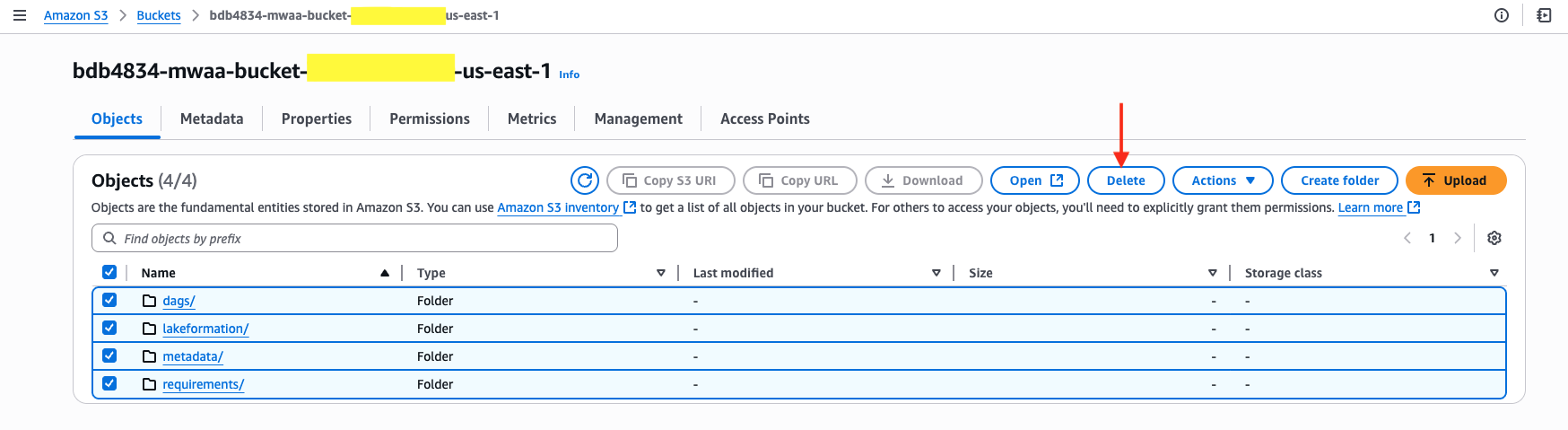
1. Open the S3 console and delete all objects from below buckets:

  • bdb4834-raw-bucket-<aws-account-id>-<region>
  • bdb4834-formatted -bucket-<aws-account-id>-<region>
  • bdb4834-mwaa-bucket-<aws-account-id>-<region>
  • bdb4834-published-bucket-<aws-account-id>-<region>

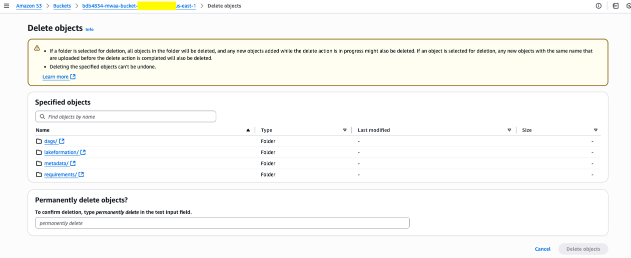
To delete all objects, choose the bucket name, select all objects and choose Delete.

After that, type ‘permanently delete’ in the text box and choose Delete Objects.

Do this for all three buckets mentioned above.

2. Go to the AWS Cloudformation console, choose you’re the stack name and select Delete. It may take approximately 40 mins for the deletion to complete.

Recommendations

When using dbt with MWAA, some typical challenges include worker resource exhaustion, dependency management issues, and in some rare cases, issues like DAGs disappearing and re-appearing when there are a large number of dynamic DAGs being created from a single python script.

To mitigate these issues, follow these best practices:

1. Scale the MWAA environment appropriately by upgrading the environment class as required.

2. Use custom requirements.txt and proper dbt adapter configuration to ensure consistent environments.

3. Set airflow configuration parameters to tune the performance of MWAA.

Conclusion

In this post, we explored the end-to-end setup of a governed data lake using MWAA and dbt which improved data quality, security, and compliance, leading to better decision-making and increased operational efficiency. We also covered how to build custom dbt frameworks for auditing and data quality, automate Lake Formation access control, and dynamically generate MWAA DAGs based on dbt tags. These capabilities enable a scalable, secure, and automated data lake architecture, streamlining data governance and orchestration.

For further exploring, refer to From data lakes to insights: dbt adapter for Amazon Athena now supported in dbt Cloud


About the authors

Muralidhar Reddy

Muralidhar Reddy

Muralidhar is a Delivery Consultant at Amazon Web Services (AWS), helping customers build and implement data analytics solution. When he’s not working, Murali is an avid bike rider and loves exploring new places.

Abhilasha Agarwal

Abhilasha Agarwal

Abhilasha is an Associate Delivery Consultant at Amazon Web Services (AWS), support customers in building robust data analytics solutions. Apart from work, she loves cooking and trying out fun outdoor experiences.

Manage data transformations with dbt in Amazon Redshift

Post Syndicated from Randy Chng original https://aws.amazon.com/blogs/big-data/manage-data-transformations-with-dbt-in-amazon-redshift/

Amazon Redshift is a fully managed, petabyte-scale data warehouse service in the cloud. You can start with just a few hundred gigabytes of data and scale to a petabyte or more. Amazon Redshift enables you to use your data to acquire new insights for your business and customers while keeping costs low.

Together with price-performance, customers want to manage data transformations (SQL Select statements written by data engineers, data analysts, and data scientists) in Amazon Redshift with features including modular programming and data lineage documentation.

dbt (data build tool) is a framework that supports these features and more to manage data transformations in Amazon Redshift. There are two interfaces for dbt:

  • dbt CLI – Available as an open-source project
  • dbt Cloud – A hosted service with added features including an IDE, job scheduling, and more

In this post, we demonstrate some features in dbt that help you manage data transformations in Amazon Redshift. We also provide the dbt CLI and Amazon Redshift workshop to get started using these features.

Manage common logic

dbt enables you to write SQL in a modular fashion. This improves maintainability and productivity because common logic can be consolidated (maintain a single instance of logic) and referenced (build on existing logic instead of starting from scratch).

The following figure is an example showing how dbt consolidates common logic. In this example, two models rely on the same subquery. Instead of replicating the subquery, dbt allows you to create a model for the subquery and reference it later.

Manage common subquery in dbt

Figure 1: Manage common subquery in dbt

The concept of referencing isn’t limited to logic related to subqueries. You can also use referencing for logic related to fields.

The following is an example showing how dbt consolidates common logic related to fields. In this example, a model applies the same case statement on two fields. Instead of replicating the case statement for each field, dbt allows you to create a macro containing the case statement and reference it later.

Manage common case statement in dbt

Figure 2: Manage common case statement in dbt

How is a model in dbt subsequently created in Amazon Redshift? dbt provides you with the command dbt run, which materializes models as views or tables in your targeted Amazon Redshift cluster. You can try this out in the dbt CLI and Amazon Redshift workshop.

Manage common data mappings

Although you can use macros to manage data mappings (for example, mapping “1” to “One” and “2” to “Two”), an alternative is to maintain data mappings in files and manage the files in dbt.

The following is an example of how dbt manages common data mappings. In this example, a model applies one-to-one data mappings on a field. Instead of creating a macro for the one-to-one data mappings, dbt allows you to create a seed for the one-to-one data mappings in the form of a CSV file and then reference it later.

Manage common data mapping in dbt

Figure 3: Manage common data mapping in dbt

You can create or update a seed with a two-step process. After you create or update a CSV seed file, run the command dbt seed to create the CSV seed as a table in your targeted Amazon Redshift cluster before referencing it.

Manage data lineage documentation

After you have created models and seeds in dbt, and used dbt’s referencing capability, dbt provides you with a method to generate documentation on your data transformations.

You can run the command dbt docs generate followed by dbt docs serve to launch a locally hosted website containing documentation on your dbt project. When you choose a model on the locally hosted website, information about the model is displayed, including columns in the final view or table, dependencies to create the model, and the SQL that is compiled to create the view or table. The following screenshot shows an example of this documentation.

Documentation generated by dbt

Figure 4: Documentation generated by dbt

You can also visualize dependencies for improved navigation of documentations during impact analysis. In the following example graph, we can see that model rpt_tech_all_users is built referencing the model base_public_users, which in turn references the table users in the public schema.

Data lineage visualization generated by dbt

Figure 5: Data lineage visualization generated by dbt

Conclusion

This post covered how you can use dbt to manage data transformations in Amazon Redshift. As you explore dbt, you will come across other features like hooks, which you can use to manage administrative tasks, for example, continuous granting of privileges.

For a hands-on experience with dbt CLI and Amazon Redshift, we have a workshop with step-by-step instructions to help you create your first dbt project and explore the features mentioned in this post—models, macros, seeds, and hooks. Visit dbt CLI and Amazon Redshift to get started.

If you have any questions or suggestions, leave your feedback in the comments section. If you need any further assistance to optimize your Amazon Redshift implementation, contact your AWS account team or a trusted AWS partner.


About the authors

Randy Chng is an Analytics Acceleration Lab Solutions Architect at Amazon Web Services. He works with customers to accelerate their Amazon Redshift journey by delivering proof of concepts on key business problems.

Sean Beath is an Analytics Acceleration Lab Solutions Architect at Amazon Web Services. He delivers proof of concepts with customers on Amazon Redshift, helping customers drive analytics value on AWS.