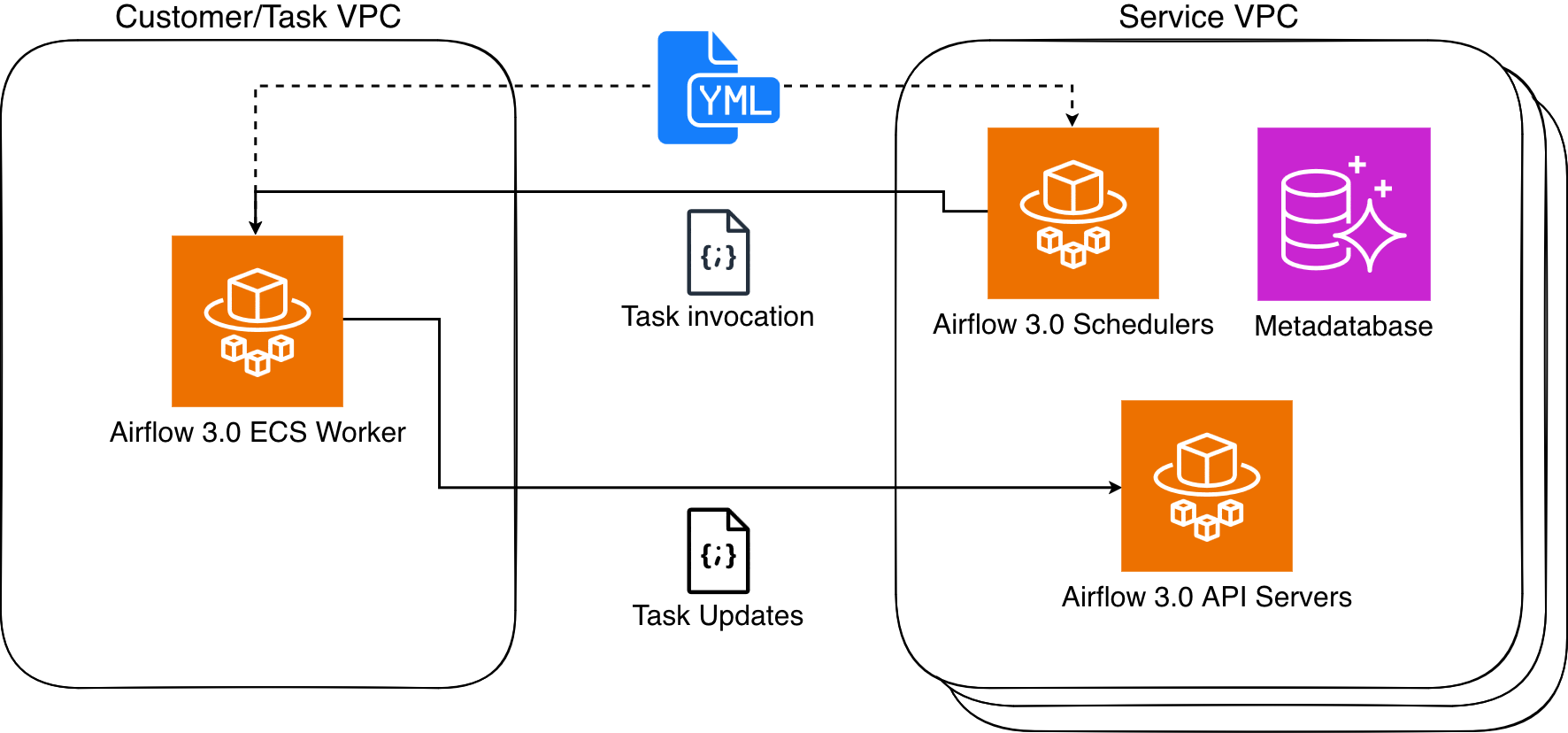
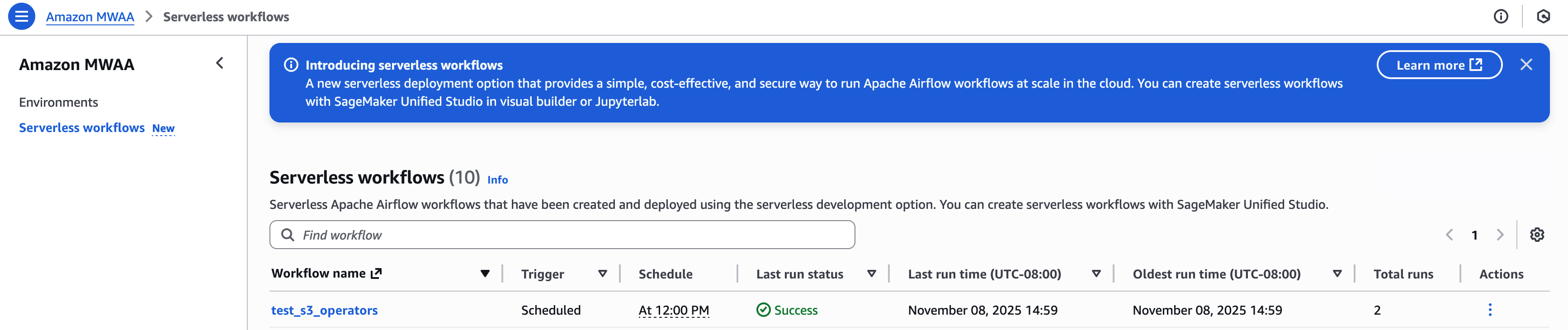
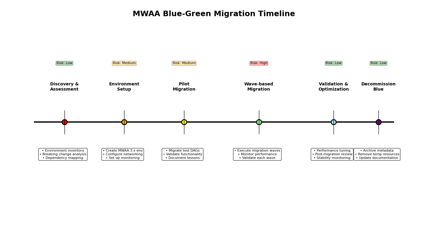
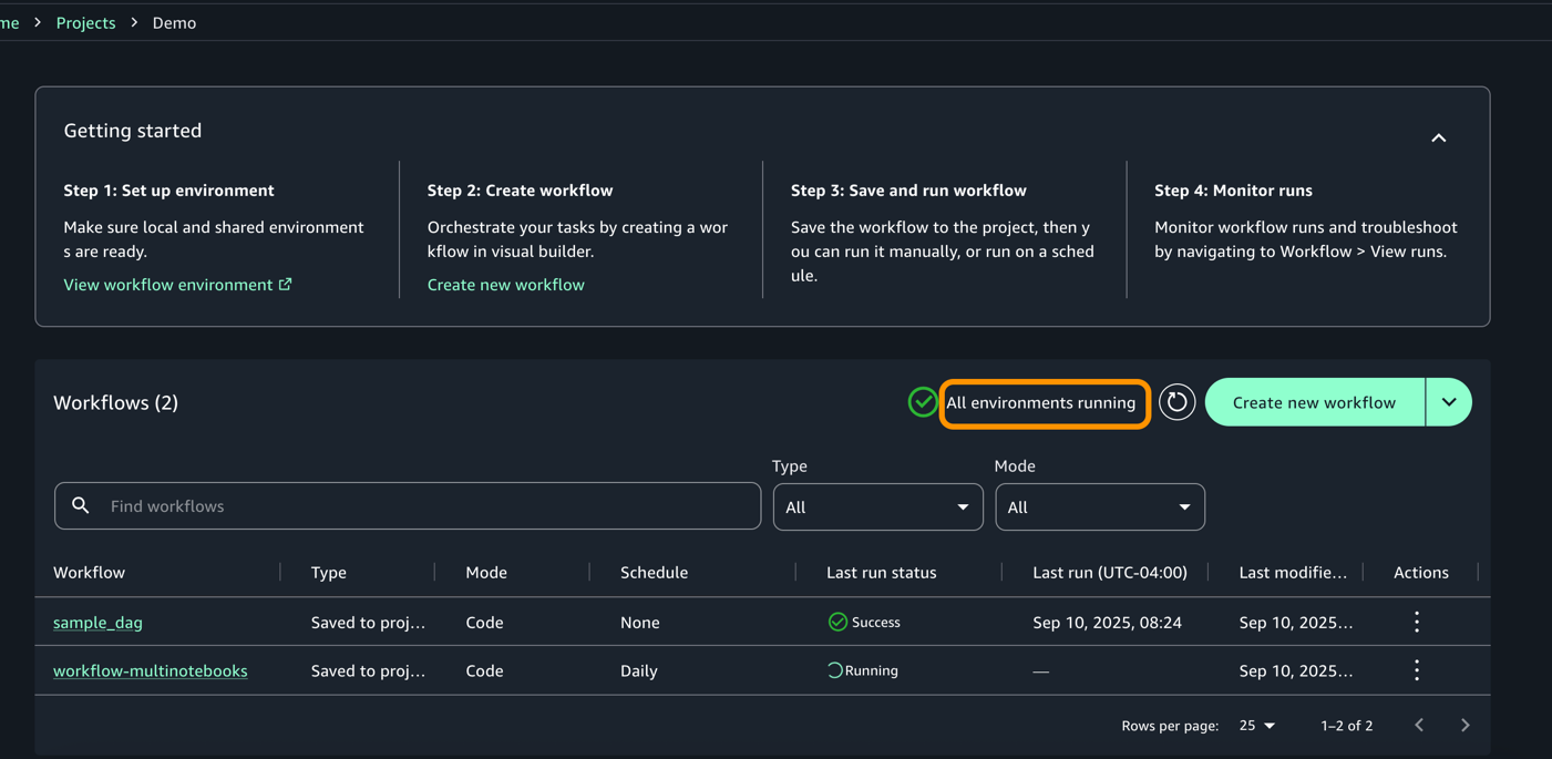
Tag Archives: Amazon Managed Workflows for Apache Airflow (Amazon MWAA)

PythonOperator and BashOperator Now Available on Amazon Managed Workflows for Apache Airflow (Amazon MWAA) Serverless

Post Syndicated from Pradeep Kumar Nalluri original https://aws.amazon.com/blogs/big-data/pythonoperator-and-bashoperator-now-available-on-amazon-managed-workflows-for-apache-airflow-amazon-mwaa-serverless/

If you run Apache Airflow workflows on Amazon MWAA Serverless, you can now use PythonOperator and BashOperator to run custom code directly in the serverless runtime. Previously, Amazon Managed Workflows for Apache Airflow (Amazon MWAA) Serverless only supported orchestration of AWS services through operators for scheduling tasks, managing dependencies, and handling retries. It did not support running your own Python functions or shell scripts natively. If you needed custom Python logic or shell commands, you had to wrap code in AWS Lambda functions, start Amazon Elastic Container Service (Amazon ECS) tasks, or use other AWS compute services. These alternatives add complexity, cost, and latency to your orchestration pipelines.

With this launch, you can run custom Python functions and shell scripts directly within the serverless task runtime, without requiring additional infrastructure. This means you can now use PythonOperator and BashOperator many data engineering teams rely on for ETL pipelines and data quality checks – without provisioning additional compute.

In this post, we walk through how this feature works and demonstrate a practical example: building a serverless pipeline that converts CSV files to JSON format using a PythonOperator, and verifies the output using a BashOperator. By the end, you will know how to:

  • Package a Python module with dependencies and upload it to an Amazon Simple Storage Service (Amazon S3) bucket as a code bundle
  • Define a multi-task workflow using the dag-factory compatible YAML
  • Create and run a workflow with the AWS Command Line Interface (AWS CLI)
  • Verify that your pipeline produced the expected output

How it works

With MWAA Serverless, you can package your custom code, upload it to an Amazon S3 bucket, and reference it when creating a workflow. The service snapshots your code at workflow creation time and uses that snapshot for all subsequent runs of the same workflow version.

Code bundles

A code bundle is the package that contains your custom logic. You package your Python modules or shell scripts and upload them to an Amazon S3 bucket. A code bundle can be:

  • A single .py file or .sh bash script (uploaded to an Amazon S3 bucket)
  • A ZIP archive containing multiple shell scripts, Python modules and dependencies (up to 250 MB)

Execution model

When you create or update a workflow, MWAA Serverless snapshots your code bundle from an Amazon S3 bucket provided and stores it on the service side. At task execution time, the service uses this snapshot – not the object currently residing in your Amazon S3 bucket – to run your code in an isolated runtime environment.

Python and Bash tasks do not have internet access. They can reach only Amazon S3, Amazon Elastic Container Registry (Amazon ECR), and Amazon CloudWatch, which are the services the runtime requires to operate. To have internet access, configure the workflow with Amazon VPC so that it can go through the provided VPC.

Supported operators

The following table describes the two operators now available in MWAA Serverless.

Operator Description
PythonOperator Executes a Python callable (function) from your code bundle
BashOperator Runs shell commands or scripts

Security

AWS Key Management Service (AWS KMS) encrypts your code bundles at rest. IAM policies control who can create, update, and trigger the workflows. The execution role scopes what AWS resources your code can access at runtime.

Prerequisites

Before getting started, verify that you have the following resources and tools configured in your AWS account:

  • An AWS account with access to Amazon MWAA Serverless
  • AWS CLI v2 (latest version) installed and configured. To install or update, see Installing or updating to the latest version of the AWS CLI.
  • An Amazon S3 bucket for storing DAG definitions and code bundles
  • An IAM role that MWAA Serverless can assume (see the execution role setup below)

Walkthrough: Building a serverless CSV-to-JSON pipeline

In this walkthrough, we build a pipeline that converts CSV files to JSON format – a common data transformation for downstream APIs and analytics systems that consume JSON. The pipeline uses a PythonOperator for the conversion logic and a BashOperator to verify the output. Here is what the pipeline does:

  1. Reads a CSV file from an Amazon S3 bucket
  2. Converts it to JSON format with column type inference
  3. Writes the JSON file back to an Amazon S3 bucket
  4. Validates record counts match between source and output

Step 1: Create the execution role

Create an IAM role that your workflow assumes at runtime. The trust policy must allow the airflow-serverless.amazonaws.com service to assume the role:

cat > trust-policy.json << 'EOF'
{
  "Version": "2012-10-17",
  "Statement": [
    {
      "Effect": "Allow",
      "Principal": {
        "Service": "airflow-serverless.amazonaws.com"
      },
      "Action": "sts:AssumeRole"
    }
  ]
}
EOF

Create the role and attach an inline policy granting least-privilege access to your S3 bucket:

aws iam create-role \
  --role-name MWAAServerlessExecutionRole \
  --assume-role-policy-document file://trust-policy.json

aws iam put-role-policy \
  --role-name MWAAServerlessExecutionRole \
  --policy-name MWAAServerlessAccessPolicy \
  --policy-document '{
  "Version": "2012-10-17",
  "Statement": [
    {
      "Effect": "Allow",
      "Action": [
        "s3:GetObject",
        "s3:PutObject",
        "s3:ListBucket"
      ],
      "Resource": [
        "arn:aws:s3:::amzn-s3-demo-mwaa-data",
        "arn:aws:s3:::amzn-s3-demo-mwaa-data/*"
      ]
    },
    {
      "Effect": "Allow",
      "Action": [
        "logs:CreateLogGroup",
        "logs:CreateLogStream",
        "logs:PutLogEvents",
        "logs:DescribeLogStreams",
        "logs:GetLogEvents"
      ],
      "Resource": "arn:aws:logs:*:*:log-group:/aws/mwaa-serverless/*"
    }
  ]
}'

Step 2: Write the Python module

Create a file called csv_to_json.py with the conversion logic:

# csv_to_json.py
import csv
import json
import boto3
import io

def convert(**kwargs):
    """Read a CSV from S3 and write it back as JSON lines."""
    bucket = "amzn-s3-demo-mwaa-data"
    source_key = "raw/sales_data.csv"
    output_key = "processed/sales_data.json"

    s3 = boto3.client("s3")

    # Read source file
    response = s3.get_object(Bucket=bucket, Key=source_key)
    content = response["Body"].read().decode("utf-8")

    # Parse CSV
    reader = csv.DictReader(io.StringIO(content))
    rows = list(reader)

    # Type inference - convert numeric fields
    for row in rows:
        for key, value in row.items():
            try:
                row[key] = float(value)
            except (ValueError, TypeError):
                pass

    # Write as JSON lines
    output = "\n".join(json.dumps(row) for row in rows) + "\n"
    s3.put_object(Bucket=bucket, Key=output_key, Body=output.encode("utf-8"))

    print(f"Converted {len(rows)} rows to JSON lines")
    print(f"Output: s3://amzn-s3-demo-mwaa-data/{output_key}")
    return {"rows": len(rows), "output_key": output_key}

This function uses boto3 (which comes pre-installed with the MWAA Serverless execution environment) and Python’s built-in csv and json modules. The conversion reads the CSV, infers numeric types, and writes a JSON lines file back to the S3 bucket.

Step 3: Write the verification script

Create a file called verify_output.sh. This script validates the pipeline output by comparing the record count in the source CSV against the output JSON file. If the counts do not match, the task fails with a non-zero exit code, which causes the workflow run to fail.

#!/bin/bash
echo "=== Data Validation ==="

# Count source records (skip CSV header)
SOURCE_COUNT=$(python3 -m awscli s3 cp s3://amzn-s3-demo-mwaa-data/raw/sales_data.csv - | tail -n +2 | wc -l)
echo "Source CSV records: $SOURCE_COUNT"

# Count output records
OUTPUT_COUNT=$(python3 -m awscli s3 cp s3://amzn-s3-demo-mwaa-data/processed/sales_data.json - | wc -l)
echo "Output JSON records: $OUTPUT_COUNT"

# Validate counts match
if [ "$SOURCE_COUNT" -ne "$OUTPUT_COUNT" ]; then
    echo "FAILED: Record count mismatch (source=$SOURCE_COUNT, output=$OUTPUT_COUNT)"
    exit 1
fi

echo "PASSED: Record counts match ($OUTPUT_COUNT records)"
echo "Timestamp: $(date -u +%Y-%m-%dT%H:%M:%SZ)"

This script runs the AWS CLI, which is bundled as a dependency in the code package. The s3 cp streams the file content to stdout without writing to disk, allowing standard shell tools like wc -l and tail to process it. The execution role credentials are automatically available in the execution environment, so the CLI can access S3 without additional configuration.

Step 4: Package and upload the code to Amazon S3

Since the verification script uses the AWS CLI, bundle it as a dependency in the ZIP archive along with your Python module and shell script:

BUCKET="amzn-s3-demo-mwaa-data"
REGION="us-east-1"

# Install awscli into a package directory
pip install awscli \
  --target my_package/ \
  --platform manylinux2014_x86_64 \
  --python-version 3.12 \
  --only-binary=:all:

# Add your module
cp csv_to_json.py my_package/
cp verify_output.sh my_package/

# Create the ZIP archive
cd my_package && zip -r ../code_bundle.zip . && cd ..
# Upload to S3
aws s3 cp code_bundle.zip s3://$BUCKET/code/code_bundle.zip --region $REGION

Upload a sample CSV file for testing:

cat > sales_data.csv << 'EOF'
date,region,product,units,revenue
2026-07-01,us-east,widget-a,150,4500.00
2026-07-01,eu-west,widget-b,89,2670.00
2026-07-02,us-east,widget-a,203,6090.00
2026-07-02,ap-south,widget-c,67,1340.00
2026-07-03,us-east,widget-b,178,5340.00
EOF

aws s3 cp sales_data.csv s3://$BUCKET/raw/sales_data.csv --region $REGION

Step 5: Define the DAG (YAML)

MWAA Serverless uses a declarative YAML format for DAG definitions. Create a file called conversion_dag.yaml:

csv_to_json_pipeline:
  start_date: "2026-01-01"
  schedule: null
  tasks:
    convert_to_json:
      operator: airflow.operators.python.PythonOperator
      python_callable: csv_to_json.convert
    verify_output:
      operator: airflow.operators.bash.BashOperator
      bash_command: "verify_output.sh"
      dependencies:
        - convert_to_json

This DAG defines two tasks:

  • convert_to_json – Runs the convert function from the Python module to transform CSV to JSON lines.
  • verify_output – Runs a shell script that validates the pipeline output by comparing source and output record counts, failing the task if they do not match.

Upload the DAG definition to S3. Note: You can also run inline Bash commands directly without a shell script.

aws s3 cp conversion_dag.yaml s3://$BUCKET/dags/conversion_dag.yaml --region $REGION

Step 6: Create the workflow

Create the MWAA Serverless workflow, referencing the DAG definition and the code bundle:

ROLE_ARN="arn:aws:iam::<your-account-id>:role/MWAAServerlessExecutionRole"

aws mwaa-serverless create-workflow \
  --name csv-to-json-workflow \
  --definition-s3-location Bucket="$BUCKET",ObjectKey="dags/conversion_dag.yaml" \
  --code '{"S3Location": {"Bucket":"'"$BUCKET"'","ObjectKey":"code/code_bundle.zip"}}' \
  --role-arn $ROLE_ARN \
  --region $REGION

The response includes a WorkflowArn that you use to trigger runs:

{
  "WorkflowArn": "arn:aws:airflow-serverless:us-east-1:123456789012:workflow/csv-to-json-workflow-abc123",
  "CreatedAt": "2026-07-15T10:30:00.000000+00:00",
  "WorkflowVersion": "a1b2c3d4e5f6"
}

Step 7: Run the workflow

Trigger a workflow run:

WORKFLOW_ARN="arn:aws:airflow-serverless:us-east-1:123456789012:workflow/csv-to-json-workflow-abc123"

aws mwaa-serverless start-workflow-run \
  --workflow-arn $WORKFLOW_ARN \
  --region $REGION

The response confirms the run has started:

{
  "RunId": "6OZV9ABF9enHKXk",
  "Status": "STARTING"
}

Step 8: Monitor execution

Check the status of your run:

RUN_ID="6OZV9ABF9enHKXk"

aws mwaa-serverless get-workflow-run \
  --workflow-arn $WORKFLOW_ARN \
  --run-id $RUN_ID \
  --region $REGION

A successful run returns:

{
  "RunDetail": {
    "Duration": 45,
    "RunState": "SUCCESS",
    "TaskInstances": ["ex_abc123_convert_to_json_1", "ex_abc123_verify_output_1"]
  },
  "RunId": "6OZV9ABF9enHKXk",
  "RunType": "ON_DEMAND",
  "WorkflowArn": "arn:aws:airflow-serverless:us-east-1:123456789012:workflow/csv-to-json-workflow-abc123",
  "WorkflowVersion": "a1b2c3d4e5f6"
}

Step 9: Verify the output

Confirm the JSON file was written to the S3 bucket:

# List the output file
aws s3 ls s3://$BUCKET/processed/sales_data.json --region $REGION

You should see the JSON file:

2026-07-15 10:32:45 1847 sales_data.json

You can also verify task-level output in Amazon CloudWatch Logs. Open the log group for your workflow and find the convert_to_json task log stream:

Converted 5 rows to JSON lines
Output: s3://amzn-s3-demo-mwaa-data/processed/sales_data.json

Considerations and limits

When planning your workloads on MWAA Serverless with these operators, keep the following considerations in mind:

  • Code bundle size – ZIP archives must be under 250 MB per bundle.
  • Network access – Python and Bash tasks do not have internet access. They can reach a limited set of AWS services required for the runtime to function (Amazon S3, Amazon ECR, and Amazon CloudWatch) but cannot call other AWS services or external endpoints. If your workflow requires calls to external APIs, preprocess that data and store it in an Amazon S3 bucket before invoking the workflow.
  • Runtime dependencies – boto3 and the Python standard library are pre-installed. For additional packages (such as pandas or requests), bundle them in your ZIP archive following the Amazon MWAA Serverless packaging guidelines.
  • Execution timeout – Tasks are subject to the workflow’s configured timeout limits.
  • Python version – Check the Amazon MWAA Serverless documentation for the currently supported Python runtime version.
  • DAG format – MWAA Serverless uses YAML-based DAG definitions, not traditional Python DAG files. If you are migrating from MWAA Provisioned, you will need to convert your DAGs to the YAML format.
  • Operators not supported – Some Airflow community operators and custom plugins are not available in the Serverless runtime. Refer to the documentation for the full compatibility list.

Clean up

To avoid ongoing charges, delete the resources you created in this walkthrough. The following commands remove the workflow, S3 objects, and IAM role:

Note: $WORKFLOW_ARN is defined in Step 7.

# Delete the workflow
aws mwaa-serverless delete-workflow \
  --workflow-arn $WORKFLOW_ARN \
  --region $REGION

Note: $BUCKET is exported in Step 4. If appropriate, delete the bucket as well.

# Remove S3 objects
aws s3 rm s3://$BUCKET/code/code_bundle.zip
aws s3 rm s3://$BUCKET/dags/conversion_dag.yaml
aws s3 rm s3://$BUCKET/raw/sales_data.csv
aws s3 rm s3://$BUCKET/processed/sales_data.json
# Delete the IAM role
aws iam delete-role-policy \
  --role-name MWAAServerlessExecutionRole \
  --policy-name MWAAServerlessAccessPolicy

aws iam delete-role --role-name MWAAServerlessExecutionRole

Conclusion

With native support for PythonOperator and BashOperator, you can now run the custom code execution patterns that many data engineering teams rely on daily directly in MWAA Serverless. Run data transformations, format conversions, validations, and shell scripts in the serverless runtime – without provisioning additional compute or managing containers.

If you are running Airflow workloads on MWAA Provisioned or self-managed infrastructure, your existing PythonOperator and BashOperator logic requires minimal changes. Convert your Python DAG files to the YAML format, package your code as a bundle, and you are ready to run on MWAA Serverless.

To get started, visit the Amazon MWAA Serverless documentation and try the walkthrough earlier in this post with your own data. For pricing details, visit the Amazon MWAA pricing page. We look forward to your feedback.


About the authors

Pradeep Kumar Nalluri

Pradeep is a Software Development Engineer at AWS, specializing in architecting and developing scalable applications. In his free time, he enjoys watching TV shows and movies.

Karthik Seshadri

Karthik is a Sr. Software Development Engineer at AWS, where he specializes in orchestration of big data technologies. He is enthusiastic about serverless technologies, data engineering and building scalable services. Outside of work, he enjoys traveling and playing various sports.

Aritra Ghosh

Aritra is a Senior Product Manager at Amazon Web Services (AWS), where he leads product development for Amazon Managed Workflows for Apache Airflow (Amazon MWAA) and Amazon SageMaker Unified Studio. Outside of work, Aritra enjoys playing squash and hitting the gym.

Sriram Ramarathnam

Sriram is a Software Development Manager on the AWS Glue, AWS Data Pipeline and Managed Serverless Airflow team in AWS Analytics. His team works on solving challenging problems in orchestration space across serverless and provisioned compute offerings.

Event-driven pipeline orchestration with Amazon MWAA and Airflow 3.0

Post Syndicated from Satya Chikkala original https://aws.amazon.com/blogs/big-data/event-driven-pipeline-orchestration-with-amazon-mwaa-and-airflow-3-0/

Data engineering teams running Apache Airflow across multiple AWS accounts face a persistent coordination problem. They have no built-in way to coordinate workflows between their separate Amazon Managed Workflows for Apache Airflow (Amazon MWAA) environments, where each team or business unit manages its own isolated environment. Cross-environment orchestration has traditionally relied on time-based polling, complex custom sensors, or API-based triggers that introduce latency and reliability concerns. The Apache Airflow Datasets feature (introduced in version 2.4) added data-aware scheduling of Directed Acyclic Graphs (DAGs, the workflow definitions that specify tasks and their execution order) within a single Amazon MWAA environment. However, teams running Airflow across multiple accounts still had no way to coordinate workflows between environments.
With Apache Airflow 3.0, now available on Amazon MWAA 3.0, you get event-driven cross-account orchestration that responds to upstream events as they happen, without polling overhead or tight environment coupling. Using Amazon Simple Queue Service (Amazon SQS) as the message broker, Asset Watchers replace polling-based sensors with event-driven triggers. This approach reduces orchestration latency from minutes to seconds and reclaims worker resources previously consumed by polling sensors. It also improves message reliability, because Amazon SQS retains coordination signals even when the consumer environment is temporarily unavailable.

In this post, you learn how to design and deploy cross-account orchestration patterns using asset-based scheduling in Airflow 3.0 with Amazon SQS integration. You learn about Asset Watchers, how to publish asset events from producer DAGs, and how to trigger dependent workflows in downstream Amazon MWAA environments, creating responsive, decoupled pipelines that span multiple accounts.

If you use AI coding assistants to build and deploy infrastructure, the solution repository includes an agent skill built on the Agent Skills standard that encodes the architecture and best practices from this post.

Solution overview

This solution demonstrates a multi-MWAA orchestration architecture where:

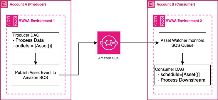
  1. Producer Amazon MWAA Environment (Account A) runs data processing workflows that publish asset events to an Amazon SQS queue when datasets are created or updated.
  2. Amazon SQS Queue acts as a message broker, decoupling producer and consumer environments.

  3. Consumer Amazon MWAA Environment (Account B) monitors the Amazon SQS queue using Asset Watchers and automatically triggers downstream DAGs when relevant asset events arrive.

Key benefits

This event-driven approach offers several advantages over traditional polling:

  • No more polling overhead: You replace continuous sensor polling with event-driven Asset Watchers that respond as events arrive.
  • Near real-time response: Downstream DAGs trigger within seconds rather than waiting for a scheduled polling interval.
  • Independent environments: Producer and consumer Amazon MWAA environments have no direct dependencies, so each team can scale and update their environment without affecting the other.
  • Reliable message delivery: Amazon SQS provides durable message delivery, even if the consumer environment is temporarily unavailable.
  • Clear team ownership: You and your team maintain your own Amazon MWAA environment while still coordinating complex cross-account workflows.
  • Faster implementation: Describe requirements in natural language and the agent skill generates deployment-ready producer and consumer DAGs with the best practices from this post built in.

Architecture overview

The following architecture shows how you can connect separate Amazon MWAA environments across AWS accounts so that a completed pipeline in one environment automatically triggers dependent workflows in another, without direct environment coupling or polling overhead.

Producer Amazon MWAA environment publishing asset events to an Amazon SQS queue that a consumer environment monitors with an Asset Watcher to trigger downstream DAGs

Figure 1: Cross-account event-driven orchestration between Amazon MWAA environments using Amazon SQS

Architecture components

The architecture has four main components. The producer DAG defines assets as outlets and publishes events to an Amazon SQS queue when tasks complete successfully. The Amazon SQS queue acts as a durable message broker between accounts, with AWS Identity and Access Management (IAM) policies granting the producer permission to send messages and the consumer permission to receive them. On the consumer side, an Asset Watcher monitors the queue and updates asset state when messages arrive, which automatically triggers the consumer DAG scheduled on that asset.
Prerequisites

Before implementing this solution, you need:

  • Two Amazon MWAA environments running Apache Airflow 3.0 or later, in the same or different AWS accounts. Each environment must have the triggerer component enabled.
  • Intermediate knowledge of IAM policies, including cross-account role trust relationships and resource-based policies.
  • Intermediate knowledge of Apache Airflow DAG authoring, including Python-based DAG definitions and task operators.
  • Basic Python experience (Python 3.8 or later) to read and adapt the provided code samples.
  • An Amazon SQS standard queue with cross-account permissions configured (see the Cross-account IAM section).
  • AWS Command Line Interface (AWS CLI) configured with credentials that have permission to access both Amazon MWAA environments and the Amazon SQS queue.
  • Time to complete: Approximately 90 minutes (following the GitHub repository instructions).
  • Estimated cost: Running two Amazon MWAA environments and an Amazon SQS queue will incur AWS charges. Refer to the Amazon MWAA pricing page and Amazon SQS pricing page to estimate costs for your Region and usage. Remember to delete resources when you finish to avoid ongoing charges.

Implementation

The post includes a GitHub repository where you can deploy the solution described in this post. You will follow the implementation steps from setting up Amazon MWAA environments and cross-account Amazon SQS queues to deploying producer and consumer DAGs with Asset Watchers. This post provides the code samples, including the DAG files, IAM policies, and requirements configuration, for demonstration purposes only. Before deploying to production, verify that you conduct thorough testing, security reviews, and validation against the specific requirements and compliance standards.

Considerations

  • Asset Watchers run as background processes in the Airflow triggerer, not the scheduler. Verify that the triggerer is healthy and running in consumer Amazon MWAA environment before expecting event-driven DAG triggers. If the triggerer is down, Amazon SQS messages will accumulate in the queue but won’t trigger downstream DAGs until the triggerer recovers. For more information, read the Asset Watchers documentation.
  • Amazon SQS messages have a default retention period of 4 days (configurable up to 14 days). If the consumer environment is unavailable for longer than the retention period, messages will be lost. Consider configuring a dead-letter queue to capture messages that fail processing, and adjust the MessageRetentionPeriod based on recovery requirements.
  • Cross-account Amazon SQS access requires both an IAM identity policy on the producer’s execution role and a resource-based policy on the Amazon SQS queue. If either policy is missing or misconfigured, message delivery will silently fail. For guidance on cross-account access patterns, refer to Four ways to grant cross-account access on AWS.
  • Set the Amazon SQS VisibilityTimeout higher than the expected time for the Asset Watcher to process a message. If the timeout is too short, messages might be redelivered and trigger duplicate DAG runs. Review the Amazon SQS visibility timeout documentation when tuning this value.
  • Each Amazon MWAA environment has limits on the number of DAGs, triggerers, and concurrent DAG runs. If you plan to scale to multiple Asset Watchers monitoring different Amazon SQS queues, check the current Amazon MWAA quotas before making design decisions.
  • Asset URIs must match exactly between the Asset Watcher definition and the consumer DAG’s schedule parameter. A mismatch, even in casing or trailing characters, will prevent the consumer DAG from being triggered. Define assets in a single DAG file to avoid inconsistencies.
  • Pin the provider packages apache-airflow-providers-amazon and apache-airflow-providers-common-messaging to versions compatible with Airflow. Incompatible versions might cause import errors that prevent the triggerer from starting. Use a constraints file as described in this post to avoid dependency conflicts.

Agent skills

AI coding assistants are most useful when they have context about your specific architecture and constraints, not only general programming patterns. Agent Skills, originally developed by Anthropic and released as a public standard in December 2025, provides a portable format for this need. SKILL.md files encode procedural knowledge, best practices, and workflows so that compatible AI coding agents can discover and apply them on demand. The standard is now supported by Kiro, Strands Agents, Anthropic Claude Code, OpenAI Codex, Cursor, Gemini CLI, and other tools. The solution provided here includes an agent skill (agent-skill/) built on this standard that encodes the cross-account orchestration architecture and operational best practices from this post. When you tell the AI coding assistant something like “Write cross-account Amazon MWAA DAGs for my orders pipeline”, the skill guides the agent through the complete workflow:

  • Collecting Amazon SQS queue URL.
  • Generating correctly structured producer and consumer DAG files.
  • Optionally deploying them to Amazon MWAA environments.

The skill doesn’t require you to provide AWS account IDs or Amazon MWAA environment names upfront. Instead, it auto-discovers your environments by running aws mwaa list-environments and aws sts get-caller-identity using the locally configured AWS CLI credentials, then asks you to confirm which environment is the producer and which is the consumer.

The skill works in two modes:

  • Sample mode: Generates the reference producer and consumer DAGs for quick cross-account validation, requiring only the Amazon SQS queue URL as input.
  • Custom mode: Adapts the DAG templates to specific business logic. For example, the producer runs an AWS Glue extract, transform, and load (ETL) job and the consumer triggers a data build tool (dbt) model refresh. This mode customizes DAG IDs, task names, schedules, and processing logic while preserving the correct Asset Watcher patterns.

Beyond code generation, the skill includes an auto-deploy flow. This flow discovers existing Amazon MWAA environments, runs pre-flight checks (Amazon Virtual Private Cloud (Amazon VPC) networking, provider versions, triggerer health, and Amazon SQS queue accessibility), uploads DAGs to the correct Amazon Simple Storage Service (Amazon S3) buckets, and verifies end-to-end readiness. Each step that modifies infrastructure requires explicit user confirmation. Also refer to the GitHub repository for instructions on using it.

Best practices

Airflow Asset Watchers with Amazon SQS are not always the right fit. When they are, they introduce operational considerations that differ from sensor-based polling approaches.

This section covers how to choose the right cross-environment orchestration pattern, how to configure the infrastructure that Asset Watchers depend on (IAM, Amazon VPC, dependencies), and how to design producer and consumer DAGs that are reliable in production.

Cross-account IAM

  • Producer execution role needs sqs:SendMessage and sqs:GetQueueUrl scoped to the specific queue ARN to avoid sqs:*.
  • Amazon SQS queue resource policy must allow the producer role for sqs:SendMessage and consumer role for sqs:ReceiveMessage, sqs:DeleteMessage, sqs:GetQueueAttributes, and sqs:GetQueueUrl.
  • Test cross-account access with the AWS CLI before deploying DAGs. Debugging AWS IAM through Airflow task logs is much harder and slower than catching misconfigurations at the CLI level.
  • Enable Amazon SQS server-side encryption for production queues.

Triggerer health

  • Airflow Asset Watchers run in the triggerer, not the scheduler. Verify triggerer health in the Airflow UI after deploying consumer DAGs.
  • The health API can report healthy even when components are broken. Cross-check by verifying Amazon CloudWatch log streams exist for the Triggerer log group.
  • Monitor airflow-<ENV>-Triggerer CloudWatch logs for ClientError, QueueDoesNotExist, or ImportError.
  • Set Amazon CloudWatch alarms on Amazon SQS ApproximateNumberOfMessagesVisible and the depth of your dead-letter queue (DLQ), which captures messages that fail processing after the maximum number of receive attempts.
  • Pin provider versions with a constraints file to prevent dependency conflicts.

Amazon VPC networking

  • Private subnets must route 0.0.0.0/0 to a NAT Gateway. Without it, workers and triggerers silently fail while the web server appears healthy.
  • Use two NAT Gateways (one per Availability Zone) for production high availability.
  • For private routing mode, use Amazon VPC Endpoints (Amazon S3, Amazon SQS, Amazon CloudWatch Logs, and Amazon Elastic Container Registry (Amazon ECR)) instead of NAT.
  • Confirm Amazon CloudWatch log streams exist for Scheduler, Worker, DAGProcessing, and Triggerer. Empty log groups mean containers aren’t running.
  • Security group must allow self-referencing inbound traffic and unrestricted outbound.

Dependency management

  • Pin provider versions with == and use a constraints file. Unpinned versions break on environment updates.
  • Test dependencies locally with MWAA Docker images before deploying.
  • Check the requirements_install_ip log stream after updates. If networking was unavailable at creation, force reinstall with a new requirements-s3-object-version.
  • Review pre-installed base packages before adding to requirements.txt to avoid version conflicts.

Choosing an orchestration pattern

Not every cross-environment dependency warrants an Asset Watcher. Airflow 3.0 offers three main orchestration patterns: Asset Watchers with Amazon SQS, the MwaaTriggerDagRunOperator, and sensor-based polling, each with different trade-offs in response time, coupling, and resource consumption. Use the following table to match your use case to the right pattern before committing to an implementation.

Pattern How it works Response time Coupling Occupies a worker? Good fit
1 Asset Watchers + SQS (this post) Consumer’s triggerer listens on SQS, triggers DAG on message arrival Seconds Loose No Cross-account pipelines. Fan-out. Independent release cycles
2 MwaaTriggerDagRunOperator Producer calls MWAA API to start a DAG in another environment Seconds Tight Yes (with wait_for_completion) Same-account one-to-one triggers
3 Sensors (polling) Consumer periodically checks for a condition Poll interval Medium Yes (unless deferrable) Persistent-state conditions. Intra-environment dependencies
  • Avoid wiring persistent-state triggers (for example, S3KeyTrigger) into Asset Watchers. They fire continuously because the condition never clears.

DAG authoring

  • Minimize module-level code. DAG files are re-parsed every cycle, and heavy imports slow the entire parsing loop.
  • Design tasks so they produce the same result whether they run once or multiple times (a property called idempotency). Duplicate Amazon SQS messages can occur on retries, so prefer UPSERT (insert or update) over INSERT to avoid duplicate records.
  • Keep secrets out of DAG files and message bodies. Use Airflow Connections (aws_conn_id) instead.
  • Test DAG imports locally with python your_dag.py before uploading to S3.
  • Allow time for DAG parsing after S3 upload, or force with dags reserialize.

Producer DAG design

  • Include dag_id, run_id, logical_date, and dataset-specific context in Amazon SQS messages so consumers can route without calling back.
  • Use SqsHook instead of the raw boto3 package. It respects aws_conn_id and integrates with Airflow logging.
  • Let publish failures raise so the Airflow retry mechanism handles redelivery.

Consumer DAG design

  • Access messages through triggering_asset_events, not by reading the queue directly. The Asset Watcher has already consumed the Amazon SQS messages.
  • Validate message payloads defensively. Producers might evolve their schema over time.
  • Use conditional asset scheduling (& / |) for complex multi-asset dependencies.

Clean up resources

To avoid ongoing AWS charges, delete the resources you created as part of this solution when you are done. The GitHub repository includes step-by-step cleanup instructions for removing the Amazon SQS queue, Amazon MWAA environments, IAM roles and policies, and Amazon S3 buckets.

Refer to the cleanup instructions in the GitHub repository to remove the provisioned resources.

Conclusion

Asset-based scheduling in Apache Airflow 3.0, with Asset Watchers, gives you a practical way to coordinate workflows across Amazon MWAA environments without polling overhead or tight coupling. By using Amazon SQS as a reliable message broker, you can build responsive, decoupled data pipelines that span multiple Amazon MWAA environments and AWS accounts without the operational overhead of traditional polling mechanisms.

This approach reduces cross-environment orchestration latency from minutes to seconds, replaces custom sensors with declarative asset-based scheduling, and gives you and your team the flexibility to maintain independent Amazon MWAA environments while still coordinating complex workflows. Amazon SQS durable message delivery reduces the risk of lost signals, even during temporary environment outages.

To get started:

  1. Review the architecture (5 minutes): Open the architecture diagram in the repository and confirm which Amazon MWAA environments will be the producer and which will be the consumer.
  2. Set up the Amazon SQS queue (15 minutes): Create a cross-account Amazon SQS standard queue and apply the IAM identity and resource-based policies from the Cross-account IAM section. Verify access with the AWS CLI before proceeding.
  3. Deploy and validate the DAG examples (30 minutes): Copy the producer and consumer DAG snippets from the Implementation section into Amazon MWAA environments, trigger the producer DAG manually, and confirm the consumer DAG runs automatically.
  4. Run pre-flight checks (20 minutes): Work through the Amazon VPC networking, provider version, and triggerer health checks in the Best Practices section. Confirm Amazon CloudWatch log streams exist for the Triggerer log group before declaring the environment ready.
  5. Optionally, use the agent skills: If you use an AI coding assistant, install the skill from the repository and describe the business logic in natural language to generate deployment-ready DAGs tailored to your pipeline.

As you scale data operations across multiple accounts and AWS Regions, asset-based scheduling with Asset Watchers provides the foundation for building modern, event-driven data architectures on AWS. Start with basic producer-consumer patterns and gradually evolve to complex multi-asset dependencies as orchestration requirements grow.

For more information, refer to


About the authors

Satya Chikkala

Satya Chikkala

Satya is a Senior Solutions Architect at Amazon Web Services, based in Melbourne, Australia. He helps enterprise customers design scalable cloud solutions that drive growth and efficiency. Outside of work, Satya trades virtual clouds for real ones – climbing rock faces, traversing mountain trails, and capturing it all through his camera lens

Corrine Tan

Corrine Tan

Corrine is a Cloud Architect at AWS specialising in data platform design across financial services, government, and startups. With a consulting background, she builds scalable, domain-oriented architectures using cloud-native technologies. Her expertise includes streaming pipelines, Airflow orchestration, data quality, and full-stack systems integrating data, models, and applications, delivering real-time platforms from ingestion to consumption

Haofei Feng

Haofei Feng

Haofei is a Senior Cloud Architect at AWS with over 20 years of expertise in DevOps, IT Infrastructure, Data Analytics, and AI. He specializes in guiding organizations through cloud transformation and generative AI initiatives, designing scalable and secure GenAI solutions on AWS. Based in Sydney, Australia, when not architecting solutions for clients, he cherishes time with his family and Border Collies.

Building a scalable personalized recommendation system on AWS: From batch to real-time

Post Syndicated from Shraddha Anil Naik original https://aws.amazon.com/blogs/big-data/building-a-scalable-personalized-recommendation-system-on-aws-from-batch-to-real-time/

Amazon.com receives millions of visits every day, and behind every product recommendation on our website is a system that needs to process customer signals, run machine learning (ML) models, and deliver results before the next visit. Doing this across global marketplaces for millions of customers at tens of thousands of requests per second, while keeping experimentation fast and infrastructure costs bounded, is an orchestration challenge as much as a machine learning one.

Our team built a system that addresses this challenge. This post shows how we did it using a batch-first architecture with AWS Lake Formation, Amazon Managed Workflows for Apache Airflow (Amazon MWAA), Amazon Athena, AWS Glue, Amazon SageMaker, and Amazon DynamoDB, and how we later extended it with Amazon MemoryDB for real-time vector similarity search when we needed to incorporate more real-time signals.

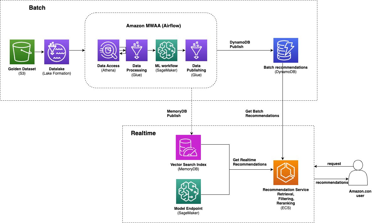
Architecture overview

Data flow from the Lake Formation data lake and Athena through Airflow-orchestrated pipelines using Glue and SageMaker into DynamoDB for batch serving and MemoryDB for real-time inference

Data flows from the centralized data lake (Lake Formation and Athena) through Airflow-orchestrated pipelines using Glue for processing and SageMaker for ML workloads, into DynamoDB for batch serving and MemoryDB for real-time inference

The data lake foundation: Centralized access with Lake Formation

Every recommendation pipeline starts with data. We built a centralized data lake to create a single source of truth that any pipeline or consumer can access without duplicating data or building bespoke extract, transform, and load (ETL) pipelines.

Golden datasets: Shared once, used everywhere

Before the data lake, each recommendation pipeline independently extracted and transformed its own copy of product catalog, transaction history, and embeddings. This led to subtle inconsistencies: one pipeline might use a slightly different join logic or a stale snapshot, making it difficult to compare model performance or debug discrepancies across pipelines.

Now, we publish curated, validated datasets once, and every consumer (Airflow DAGs, ML notebooks, analytics dashboards) reads from the same tables through the same governed access. This means:

  • New pipelines start faster. A new recommendation model does not need its own data extraction logic. It queries the existing golden datasets from day one.
  • Consistency across models. When we compare model A to model B, we know both models are trained and inferred on the same underlying data.
  • Cross-team collaboration. Multiple teams share the same tables as a single source of truth.
  • Two-way data flow. The data lake serves as both source and destination. Our pipelines read golden datasets as inputs and write computed outputs (model scores, feature sets, intermediate results) back to the lake, where they become inputs for other pipelines. This creates a compounding effect: each new pipeline enriches the lake for the next one.

Why Lake Formation?

Our data is stored in Amazon Simple Storage Service (Amazon S3), partitioned by marketplace. Our data consumers (Airflow pipelines, ML notebooks, analytics tools) live in separate AWS accounts from the data producers. We chose AWS Lake Formation because it adds governance on top of S3 without requiring data migration:

  • Fine-grained cross-account access. Grant table-level permissions per consumer role, without managing bucket policies manually.
  • Schema governance through AWS Glue Data Catalog. Scheduled Glue crawlers infer schemas from files in S3, keeping the catalog current as data evolves.
  • Multi-Region consistency. We deploy identical infrastructure across multiple AWS Regions using AWS Cloud Development Kit (AWS CDK), each Region serving its local marketplaces.

Orchestration: Amazon Managed Workflows for Apache Airflow (Amazon MWAA)

We chose Amazon Managed Workflows for Apache Airflow (Amazon MWAA) as our orchestration layer. MWAA removes the operational burden of managing Airflow infrastructure: automatic scaling of workers, built-in high availability, and managed upgrades mean our team focuses on pipeline logic rather than cluster maintenance. MWAA lets us define complex multi-step workflows with rich dependencies in Python code, and its operator model lets us encapsulate team-specific conventions into reusable building blocks.

Each recommendation pipeline follows a consistent pattern:

The consistent recommendation pipeline pattern moving from data extraction through model training, batch inference, vector search, ranking, and publishing

We built a library of reusable custom Airflow operators, each encapsulating one of our core compute engines. This reduced new pipeline development from weeks to days in our team’s experience.

Athena and AWS Glue: Data access and processing

Amazon Athena is how our pipelines read from Lake Formation. Our custom operator runs SQL queries against the Glue Data Catalog and automatically runs UNLOAD to write results to S3: serverless, no infrastructure to manage, and integrated with the Lake Formation permission model.

AWS Glue handles compute-intensive data transformations through PySpark: joining datasets, filtering, deduplication, aggregation, and formatting ML outputs into final recommendation lists. We configure Glue with Auto Scaling worker pools (for example, 2–50 workers of G.8X type) so jobs scale with data volume per marketplace. All jobs run ephemerally: they read from S3, write to S3, and require no long-running clusters.

Amazon SageMaker powers the ML-intensive stages of our pipelines across three workload types, all orchestrated as steps within our Airflow DAGs:

Training

We use SageMaker Training Jobs to train our recommendation models on GPU instances (for example, ml.g5). Training data is prepared by upstream Glue jobs and staged in S3. Our custom Airflow operator submits the training job, monitors its progress, and registers the resulting model artifact in S3. Once training completes, the artifact is immediately available for batch inference or endpoint deployment within the same DAG run. This means a single DAG can go from raw data to trained model to deployed inference without manual handoffs, and we can retrain it on fresh data every pipeline cycle with zero operator intervention.

Batch inference

SageMaker Batch Transform runs our trained models at scale, generating the outputs that feed into downstream ranking and publishing steps. Our batch inference operator handles job submission, polls for completion, and writes the output location to the DAG’s S3 convention so the next Glue step can pick it up automatically. Batch Transform lets us run inference without provisioning persistent infrastructure, and we can scale instance count and type independently for every pipeline based on data volume.

Generating recommendations for millions of customers requires searching across hundreds of thousands of candidate products per customer. Exact search at this scale is prohibitively expensive, so we use approximate nearest neighbor (ANN) search using FAISS to find similar products efficiently, run as SageMaker Processing Jobs.

The workflow:

  1. Build a FAISS index over the candidate catalog.
  2. Query the index with per-customer vectors to find top-K nearest neighbors.
  3. Return ranked candidate lists per customer.

We distribute query vectors across the SageMaker Processing fleet using S3-based sharding (ShardedByS3Key). Each instance receives the full candidate index but only a fraction of the query vectors. Every instance builds an identical FAISS index, searches its shard of queries, and writes results to S3. The downstream Glue step merges all shards into the final recommendation lists. This lets us scale horizontally by adding instances without changing any code.

Why SageMaker inside MWAA?

Running SageMaker jobs as MWAA tasks (rather than standalone) gives us:

  • End-to-end lineage. Every model training run, inference job, and vector search is tracked as part of a DAG execution. We can trace a recommendation in DynamoDB back to the exact training run, data snapshot, and ANN search that produced it.
  • Retry and failure handling. If a SageMaker job fails (spot instance preemption, transient capacity errors), Airflow retries it automatically with backoff. No manual re-runs.
  • Resource sequencing. Training must finish before inference, inference before ANN search. The Airflow dependency model handles this naturally without polling scripts or step function state machines.
  • Unified monitoring. One Airflow dashboard shows the health of all pipelines: Glue ETL, SageMaker training, SageMaker inference, and DynamoDB publishing. No context-switching between consoles.

Putting it together: A complete pipeline example

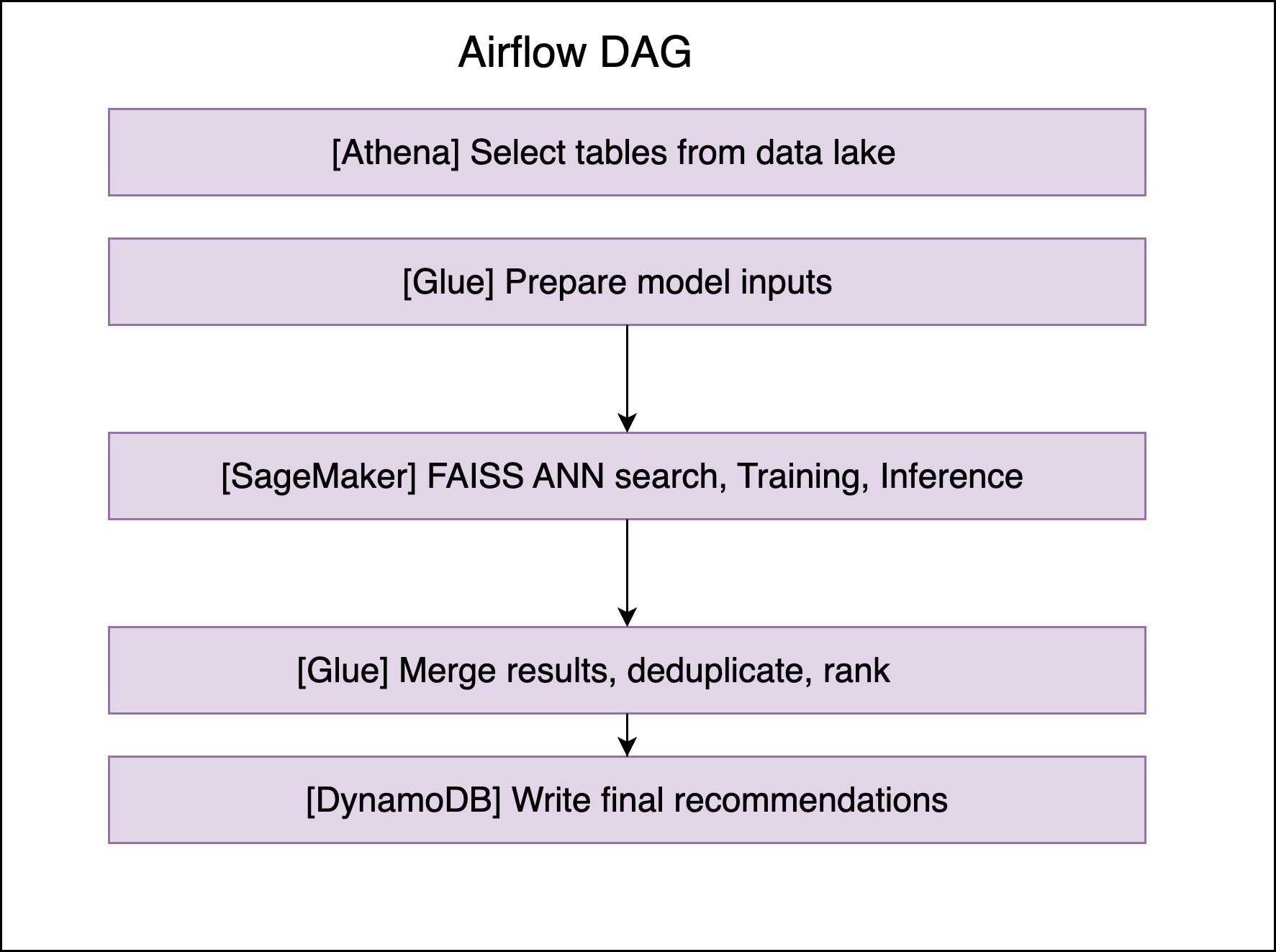
Our recommendation generation pipeline illustrates the full flow:

The complete recommendation generation pipeline: data lake extraction, model training, batch inference, vector search, merge and rank with Glue, and publishing to DynamoDB

Note that the operators shown (GlueSQLOperator, VectorSearchOperator, and others) are custom internal operators built on top of the Airflow AWS provider, not open-source libraries. Here is a simplified version of what this looks like in code:

from airflow import DAG
from airflow.models.baseoperator import chain
from airflow.utils.task_group import TaskGroup

dag = DAG("recommendation_generator", schedule="0 18 * * 4")  # Weekly
task_groups = []

for marketplace in [...]:  # global marketplaces
    with TaskGroup(group_id=marketplace, dag=dag) as group:

        # Step 1: Extract data from lake
        candidates = GlueSQLOperator(
            task_id="select_candidates",
            tables=[f"{marketplace}.catalog", f"{marketplace}.products"],
            sql="select_candidates.sql", dag=dag)

        customer_history = GlueSQLOperator(
            task_id="select_customer_history",
            tables=[f"{marketplace}.transactions"],
            sql="select_customer_vectors.sql", dag=dag)

        customers = AthenaSQLOperator(
            task_id="select_customers", database=marketplace,
            query="select_customer_cohort.sql", dag=dag)

        # Step 2: Train model
        train = ModelTrainingOperator(
            task_id="train_model",
            training_input={"task_id": customer_history.task_id},
            instance_type="ml.g5", dag=dag)

        # Step 3: Batch inference
        inference = BatchInferenceOperator(
            task_id="batch_inference",
            model={"task_id": train.task_id},
            input_data={"task_id": candidates.task_id}, dag=dag)

        # Step 4: Vector search via SageMaker Processing Job
        ann_search = VectorSearchOperator(
            task_id="ann_search",
            index_input={"task_id": inference.task_id},
            query_input={"task_id": customer_history.task_id},
            k=60, instance_count=10, dag=dag)

        # Step 5: Merge and rank with Glue
        merge_and_rank = GlueSparkOperator(
            task_id="merge_and_rank",
            script="merge_results.py", dag=dag)

        # Step 6: Publish to DynamoDB
        publish = DynamoDBPublishOperator(
            task_id="publish_recommendations",
            table_name="Recommendations", dag=dag)

        # Task dependencies
        [candidates, customer_history] >> train >> inference
        [inference, customers] >> ann_search >> merge_and_rank >> publish

    task_groups.append(group)

chain(*task_groups)  # Execute marketplaces sequentially

Key patterns in this DAG

  • Marketplace isolation. Each marketplace runs in its own TaskGroup. A failure in one does not block the others.
  • Parallel data extraction. Independent Athena/Glue queries run concurrently before converging at the training step.
  • Sequential marketplace execution. chain() runs marketplaces one at a time to avoid resource contention across large SageMaker and Glue jobs.
  • Reusable operators. We built custom operators like GlueSQLOperator, VectorSearchOperator, and DynamoDBPublishOperator that encode our team’s conventions (cross-account access, S3 staging, retry logic, metrics) into shared building blocks. New pipelines are mostly configuration rather than infrastructure code, and these operators are shared across dozens of pipelines.
  • Implicit data passing. Each operator writes its output to a convention-based S3 path and downstream operators automatically resolve the upstream output location. No hard-coded paths between steps.

This pattern powers hundreds of pipelines across global marketplaces, with each marketplace as an isolated TaskGroup in the DAG.

Serving layer: DynamoDB + ECS

Our Java-based Amazon Elastic Container Service (Amazon ECS) service reads pre-computed recommendations from Amazon DynamoDB at request time:

  1. Receive request with customer ID, marketplace, customer context, and page context.
  2. Read pre-computed recommendations from DynamoDB.
  3. Apply real-time filters (availability, eligibility constraints).
  4. Re-rank based on real-time context signals.
  5. Return the response.

Amazon DynamoDB is designed to provide single-digit millisecond reads at our scale and time-to-live (TTL) for automatic cleanup of stale recommendations.

Extending to real-time

In recommendation system terms, our batch pipeline handles the retrieval stage offline. Although this covers the majority of our traffic, we identified scenarios where weekly freshness was not enough to capture what customers are doing right now. The real-time extension adds an online retrieval and ranking path for signals that cannot wait for the next batch cycle.

To address these, we extended our system with Amazon MemoryDB (which now supports Valkey as its open-source engine) for real-time vector similarity search and SageMaker real-time endpoints for on-demand embedding generation. The same Airflow pipelines that publish to DynamoDB also publish product vectors to MemoryDB (through our MemoryDB publish operator), and the same model in our batch pipeline is deployed to a SageMaker endpoint for single-item inference at request time.

At serving time, when we want to incorporate fresh signals, the service calls the SageMaker endpoint to generate an embedding on the fly, then queries MemoryDB for the nearest neighbors. These fresh signals include recent search queries, cart additions, and other in-session activity that changes faster than our weekly batch cycle. In our workloads, this gives us sub-millisecond vector search latency without re-running the full batch pipeline. Critically, the batch pipeline keeps the MemoryDB product index fresh. Our Airflow DAG includes a MemoryDB publish operator that refreshes the full product vector index weekly, so real-time queries always search against an up-to-date index.

Batch and real-time are not competing approaches: batch handles slow-moving signals (purchase history, catalog relationships) while real-time handles fast-moving ones (current session, new arrivals, trending items). Both paths share the same models, the same data lake, and the same serving service.

For a detailed deep-dive on this real-time architecture, see Real-time personalized recommendations with Amazon SageMaker and Amazon Managed Valkey.

Security and access control

Security is a foundational concern for a system that spans multiple AWS accounts, processes customer behavioral data, and runs across multiple AWS Regions.

Cross-account access: Lake Formation grants are issued to consumer-account AWS Identity and Access Management (IAM) roles, ensuring consumers can query tables without direct S3 bucket access. Each consumer role receives only the permissions it needs for its specific tables.

IAM execution roles: Each compute engine (MWAA, Glue, SageMaker) runs under a dedicated least-privilege IAM role.

Network isolation: MWAA environments and the ECS serving layer are deployed within virtual private clouds (VPCs), with separate VPC configurations per Region.

Reliability and failure handling

Regional isolation: Each AWS Region runs an independent copy of the system. DynamoDB tables are regional, each populated by the local batch pipeline. MemoryDB clusters are regional, with the product vector index refreshed by the local Airflow DAG. This means a regional failure or pipeline delay in one Region does not affect other Regions.

Batch pipeline failures: If a pipeline fails mid-run, the previous DynamoDB data remains live and continues serving recommendations until the next successful run. Airflow retries failed tasks automatically with configurable backoff. TTL on DynamoDB records bounds how long stale data persists. Failed pipeline runs trigger automated alerting so the on-call engineer can investigate.

Real-time path resilience: MemoryDB is deployed in a multi-AZ configuration with automatic failover. The real-time path is an extension of the batch system, and batch recommendations from DynamoDB remain available regardless of real-time path availability.

Lessons learned

  1. Start batch, add real-time incrementally. Batch pipelines are easier to debug, cheaper to operate, and sufficient for most recommendation scenarios. Add real-time path only when you have clear indication that specific customer signals (for example, in-session activity, search queries) need sub-hour freshness to remain relevant.
  2. Match the serving path to signal velocity. Not every signal needs real-time processing. Categorize your signals by how quickly they change, and route accordingly: batch for slow signals, real-time for fast ones, re-ranking for in-between.
  3. Freshness does not always require re-computation. A batch-generated candidate set remains largely valid between runs. What changes is relative relevance. Re-ranking at serving time with recent customer activity gives the impression of real-time without the cost of real-time candidate generation.
  4. A centralized data lake accelerates everything. Golden datasets eliminated weeks of per-pipeline data extraction work, made model comparisons trustworthy, and let new team members ship their first pipeline in days instead of weeks. The upfront investment in Lake Formation governance paid for itself within the first quarter.
  5. Invest in reusable operators. Custom Airflow operators encapsulating Athena/Glue/SageMaker patterns let teams ship new pipelines in days. The operators encode best practices (retry logic, cross-account access, metrics) so pipeline authors can focus on business logic.
  6. Separate compute from storage. S3 as the universal intermediate layer + ephemeral Glue/SageMaker jobs means you pay only for active computation. No idle clusters between weekly pipeline runs.

Conclusion

We built this system because every customer interaction is an opportunity to surface the right product at the right time. Serving tens of thousands of requests per second across millions of customers in global marketplaces, our batch-first architecture uses AWS Lake Formation for governed data access, Amazon MWAA for orchestration, Amazon Athena for data lake queries, AWS Glue for distributed processing, Amazon SageMaker for training, inference, and vector search, and Amazon DynamoDB for low-latency serving. When we needed to incorporate more real-time signals, we added Amazon MemoryDB vector search paired with SageMaker real-time endpoints for on-demand embedding generation, extending into real-time without replacing the batch foundation.

The architecture choices we have made, batch for efficiency and real-time for freshness, all serve the goal of helping customers discover what they need faster. If you are building personalized experiences at scale, we hope these patterns give you a useful starting point.

This would not have been possible without the Everyday Essentials engineering team, whose collective effort turned these ideas into a production system serving customers every day. We are also grateful for the support and guidance from Sam Heyworth, Nirav Desai, and Ankur Datta, and the broader Everyday Essentials leadership team.


About the authors

Shraddha Anil Naik

Shraddha Anil Naik

Shraddha is a Senior Software Engineer on the Everyday Essentials team at Amazon. She specializes in retrieval and recommendation infrastructure that powers personalized experiences for millions of customers.

Sergii Oborskyi

Sergii Oborskyi

Sergii is a Senior Software Engineer on the Everyday Essentials team at Amazon. He builds online recommendation services that serve product recommendations to millions of customers at high throughput and low latency.

Shawn Liu

Shawn is a Senior Machine Learning Engineer on the Everyday Essentials team at Amazon. He develops and evaluates recommendation models on Amazon SageMaker that power personalized product discovery for millions of customers.

Walter Wong

Walter Wong

Walter is a Software Development Manager in the Everyday Essentials Science org at Amazon. His work focuses on customer understanding and personalization, improving product recommendations for millions of customers across Amazon’s everyday essentials catalog.

How Mapfre USA modernized fraud claims with Amazon EMR Serverless

Post Syndicated from Lijan Kuniyil original https://aws.amazon.com/blogs/architecture/how-mapfre-usa-modernized-fraud-claims-with-amazon-emr-serverless/

Insurance fraud remains a significant challenge for the insurance industry because fraudulent claims can increase loss costs, reduce trust, and consume investigation capacity that could otherwise be focused on serving customers. Traditional fraud detection approaches typically rely on rules-based controls, manual investigation triggers, historical claim patterns, and structured-data-only analysis. These approaches are useful for known fraud patterns, but they can struggle to detect sophisticated fraud rings or hidden relationships across claimants, policies, vehicles, providers, addresses, and prior suspicious activities.

Mapfre USA is the number one auto and home insurer in Massachusetts, serving customers in 11 states nationwide. Our coverage includes auto, home, motorcycle, watercraft, business insurance, and more. As part of Mapfre Group, we’re a worldwide leader serving over 31.1 million customers in more than 100 countries with a team of 31,000 employees. In collaboration with AWS and Neo4j, Mapfre USA modernized its fraud prevention capabilities by combining graph-based features with machine learning (ML) models deployed on AWS. This initiative, focused initially on Massachusetts Auto insurance and later expanded to Home (HO), has delivered significant business impact, exceeding $5 million Net Present Value (NPV), with realized savings already outperforming projections.

In this post, we share how Mapfre USA designed and implemented this solution, highlight the technical architecture running on AWS specifically on the Mapfre Data Platform called Atenea, and explore lessons learned that can apply to other industries facing complex fraud challenges.

Business challenge

Fraudulent claims aren’t always isolated events. They often involve hidden networks of policyholders, vehicles, providers, and prior suspicious activities. Detecting these complex relationships requires going beyond traditional structured data analysis.

Mapfre set out with a clear goal:

  • Goal: Improve fraud detection accuracy and claims handling efficiency.
  • Key KPI: Identify fraudulent claims missed by traditional methods.
  • Approach: Develop several ML models that use both traditional structured data and graph-based features derived from claim relationships.
  • Deployment: Integrate seamlessly with Guidewire Claims, so front-line adjusters automatically receive fraud alerts with explanations.

Each flagged claim exposure generates a Guidewire activity showing the top three model drivers, helping investigators understand why the claim was identified and act quickly.

Technical solution on AWS (Atenea Data Platform)

The fraud detection platform is built on a modern data architecture on AWS, designed to scale efficiently and provide long-term governance.

At its core, the solution uses Apache Iceberg tables stored on Amazon Simple Storage Service (Amazon S3), with metadata managed through the AWS Glue Data Catalog and access governed through AWS Lake Formation as part of the Atenea lakehouse governance model. The platform feature store is implemented through feature-store-managed Iceberg tables that manage model features, predictions, and Guidewire activities. The implementation is structured across three logical layers:

  • Silver Layer – Iceberg tables that contain source data from each of the sources, used as the initial consumption point of the platform.
  • Gold Layer – Iceberg tables storing intermediate data, such as unified Guidewire activity logs, Auto features, and Home features.
  • Platinum Layer – Feature Store-managed Iceberg tables containing encoded features and model predictions, making them reusable across models and ensuring strong metadata governance.

Processing pipelines are executed on Amazon EMR Serverless, with orchestration managed by Apache Airflow operators running on Amazon Managed Workflows for Apache Airflow (Amazon MWAA). This provides elastic, cost-efficient compute for both batch processing and fast-time scoring, while keeping orchestration, monitoring, and recovery centralized.

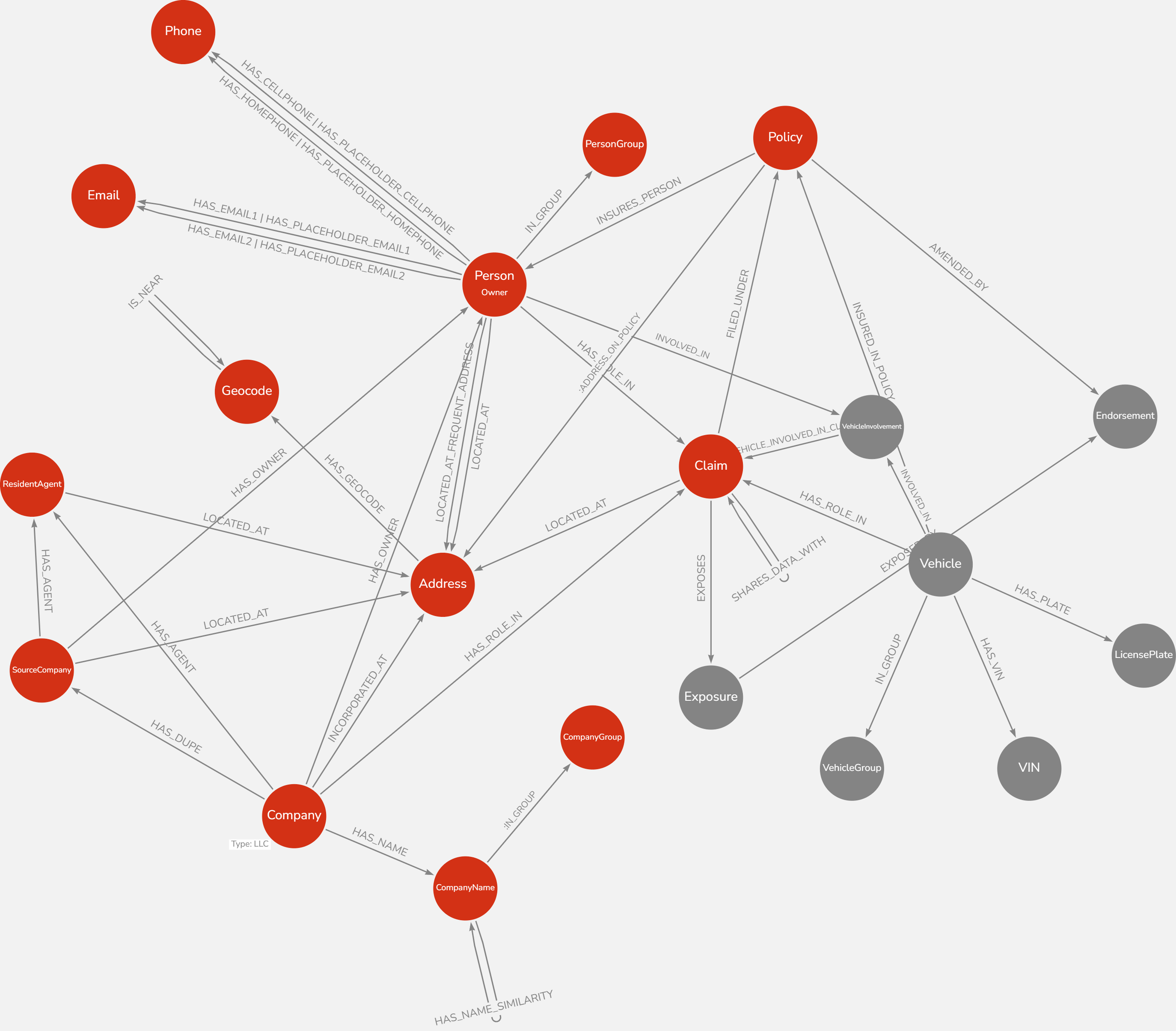
For graph enrichment, the platform connects to Neo4j using a dedicated driver, enabling advanced network-based features like suspicious claim linkages, provider fraud ratios, and centrality metrics.

This architecture supports efficient, reliable, and transparent production execution through repeatable Airflow orchestration, environment-based continuous integration and delivery (CI/CD) promotion, centralized monitoring, failure notifications, retry mechanisms, dead-letter queue handling for Guidewire integration, and controlled secret management. At the same time, the layered lakehouse design keeps the platform flexible enough to evolve with new business needs and fraud detection use cases.

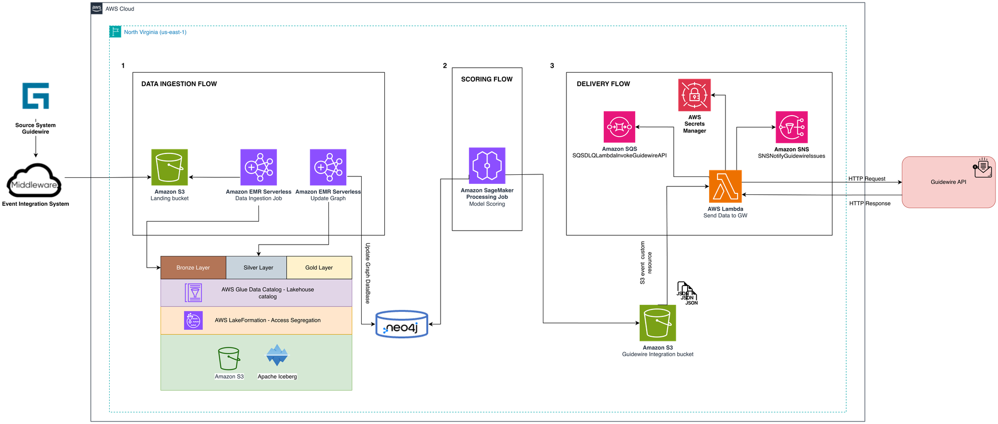
Architecture diagram showing the Mapfre USA fraud detection platform on AWS, including data ingestion, graph enrichment, model scoring, and Guidewire integration

The data sources are policy, claims, vehicles, and notes (from AS400 and Guidewire), which include structured data and derived features capturing entity relationships (graph data).

The following list describes the architecture overview:

  1. Data ingestion – Claim batch data uploaded to Amazon S3. Data gets standardized and materialized in Iceberg tables within the Silver layer.
  2. Graph enrichment – Data processed to update Neo4j graph database hosted on AWS.
  3. Model training and scoring – Batch scoring for several ML models.
  4. Model orchestration – Unified orchestration for ingestion, training, and inference using Apache Airflow operators. CI/CD pipelines for promotion across environments.
  5. Execution platform – Amazon EMR Serverless for cost-efficient Spark processing. Migration to Apache Iceberg plus AWS Glue Data Catalog for scalable metadata handling.
  6. Integration with claims systems – Fraud predictions automatically create Guidewire activities, enriched with a description for investigators.
  7. Secrets and securityAWS Secrets Manager securely stores credentials and tokens for Guidewire API integration, with environment-specific and Region-specific access controls.
  8. Monitoring and reliabilityAmazon CloudWatch and Amazon Simple Notification Service (Amazon SNS) provide visibility into pipeline health and notify teams on failures. Data quality checks are executed at key stages of the pipeline to validate data availability, schema consistency, completeness, and business-rule expectations before outputs are consumed by models or sent to Guidewire.

Guidewire integration with MLOps on AWS

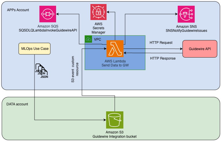
One of the most important parts of Mapfre’s solution was closing the loop between ML predictions and the claims handling system. This required a resilient integration between the Atenea data platform on AWS and Guidewire Claims.

The following describes the integration flow:

  1. When an ML use case finishes scoring, the results are written as JSON files into the S3 path: <bucket_name>/guidewire/.
  2. An S3 event notification triggers an AWS Lambda function.
  3. This Lambda function:
    • Reads the JSON file.
    • Calls the Guidewire Predictive Model API.
    • Because Guidewire doesn’t support batch requests, the Lambda function sends each JSON payload individually. This keeps the integration compatible with Guidewire and isolates failures at the individual activity level, but it increases the number of API calls and makes retry, throttling, DLQ handling, and monitoring controls important.
  4. If successful, the API responds with HTTP 201 (activity created).
    • If not, the Lambda function retries up to two times.
    • Failed requests are sent to an Amazon Simple Queue Service (Amazon SQS) dead-letter queue (DLQ), and an Amazon SNS notification is published for monitoring.
  5. Secrets are stored in AWS Secrets Manager and injected as Lambda environment variables, along with AWS Region-specific URLs for token retrieval and API endpoints.
  6. The following JSON shows the example structure for Guidewire integration:
{
  "method": "createPredictiveActivity",
  "params": [
    {
      "claimNumber": "AUXXXXXXX",
      "exposureNumber": 1,
      "subject": "Fraud alert from ML model",
      "description": "Claim flagged as potential fraud based on graph + ML features",
      "shortSubject": "ML_Fraud_Flag",
      "priority": "high",
      "availableForClosedClaim": true,
      "autoCloseOnExposureClosure": false,
      "targetDays": 4,
      "escalationDays": 6
    }
  ]
}

Diagram showing the Guidewire integration flow with AWS Lambda, Amazon SQS dead-letter queue, and AWS Secrets Manager

Key benefits of this integration:

  • Real-time actionability – Fraud predictions automatically create Guidewire activities for front-line adjusters.
  • Resilience – Built-in retries, DLQ handling, and Amazon SNS alerts make sure failed events aren’t lost.
  • Security – Secrets and tokens are managed using AWS Secrets Manager, with strict environment separation (dev, pre, pro).
  • Scalability – Any new MLOps use case writes results into the S3 output path, automatically flowing into Guidewire.

This integration shows that fraud models don’t exist in isolation but actively augment daily claim workflows in production. It connects Atenea’s MLOps pipelines on AWS directly with business decisioning systems, which is critical to realizing the fraud savings impact.

Data quality and resilience

For robustness, data quality checks are applied on ingestion pipelines and graph features. Automated validation detects anomalies early, monitoring dashboards track KPIs and model performance, and standardized recovery and promotion processes operate across environments.

Visualization and investigative tools

Neo4j Bloom supports SIU workflows by visually exploring entity relationships, such as a provider linked across multiple suspicious claims, accelerating fraud ring identification.

Conclusion

The fraud detection model in auto claims has enhanced Mapfre USA’s ability to identify fraudulent activity, driving significant savings and improving overall claims efficiency.

During the pilot phase alone, savings exceeded projections, and in production the initiative has proven a Net Present Value (NPV) of more than $5M. These results confirm the business case and highlight the strength of combining structured data with graph-based features to uncover fraud networks that traditional approaches miss.

The results have been compelling:

  • Accuracy gains – Detection improved by 50–135 percent compared to baseline methods.
  • Substantial realized value – Both during the pilot and in production.
  • Cross-functional success – The initiative brought together Claims, IT Data, Advanced Analytics, and Neo4j teams in an agile, collaborative model.

Beyond the financial outcomes, several lessons have emerged. First, cross-functional collaboration between groups like Claims, Data Engineering, Advanced Analytics, and technology partners like AWS and Neo4j was critical to success. Second, explainability proved essential. By presenting adjusters with the top model drivers directly in Guidewire, trust and adoption of the system increased substantially. Finally, building resilience into the architecture through monitoring, retries, and data quality processes helped the models operate reliably in production.

Looking ahead, the platform is well-positioned to expand beyond fraud detection. New use cases such as underwriting anomaly detection and customer entity resolution are already on the roadmap. With robust architecture built on AWS using Amazon EMR Serverless, Apache Iceberg on Amazon S3 supported by AWS Glue Data Catalog and Lake Formation, a custom-built Feature Store, and Neo4j, Mapfre now has a scalable foundation to continue driving innovation and business impact.

To learn more about Amazon EMR Serverless, see the Amazon EMR Serverless documentation.

How MAPFRE USA modernized fraud claims with Amazon EMR Serverless

Post Syndicated from Lijan Kuniyil original https://aws.amazon.com/blogs/architecture/how-mapfre-usa-modernized-fraud-claims-with-amazon-emr-serverless/

Insurance fraud remains a significant challenge for the insurance industry. Fraudulent claims can increase loss costs, reduce trust, and consume investigation capacity that could otherwise be focused on serving customers. Traditional fraud detection approaches typically rely on rules-based controls, manual investigation triggers, historical claim patterns, and structured-data-only analysis. These approaches are useful for known fraud patterns, but they can struggle to detect sophisticated fraud rings or hidden relationships across claimants, policies, vehicles, providers, addresses, and prior suspicious activities.

MAPFRE USA is a top-rated auto and home insurer in Massachusetts, serving customers in 11 states nationwide. Our coverage includes auto, home, motorcycle, watercraft, business insurance, and more. As part of MAPFRE Group, we’re a worldwide leader serving over 31.1 million customers in more than 100 countries with a team of 31,000 employees. In collaboration with AWS and Neo4j, MAPFRE USA modernized its fraud prevention capabilities by combining graph-based features with machine learning (ML) models deployed on AWS. This initiative focused initially on Massachusetts auto insurance and later expanded to home insurance. It has delivered significant business impact, exceeding $5 million in net present value (NPV) over five years, with realized savings already outperforming projections.

In this post, we share how MAPFRE USA designed and implemented this solution, highlight the technical architecture running on AWS, specifically the MAPFRE data platform called Atenea, and explore lessons learned that can apply to other industries facing complex fraud challenges.

Business challenge

Fraudulent claims aren’t always isolated events. They often involve hidden networks of policyholders, vehicles, providers, and prior suspicious activities. Detecting these complex relationships requires going beyond traditional structured data analysis.

MAPFRE set out with a clear goal:

  • Goal: Improve fraud detection accuracy and claims handling efficiency.
  • Key performance indicator (KPI): Identify fraudulent claims missed by traditional methods.
  • Approach: Develop several ML models using both traditional structured data and 54 graph-based features derived from claim relationships.
  • Deployment: Integrate with Guidewire Claims, so front-line adjusters automatically receive fraud alerts with explanations.

Each flagged claim exposure generates a Guidewire activity showing the top three model drivers, helping investigators understand why the claim was flagged and act quickly.

Technical solution on AWS (Atenea data platform)

The fraud detection platform is built on a modern data architecture on AWS, designed to scale efficiently and support long-term governance.

At its core, the solution uses Apache Iceberg tables stored on Amazon Simple Storage Service (Amazon S3), with metadata managed through the AWS Glue Data Catalog and access governed through AWS Lake Formation as part of the Atenea lakehouse governance model. The platform feature store is implemented through feature-store-managed Iceberg tables that manage model features, predictions, and Guidewire activities. The implementation is structured across three logical layers:

  • Silver layer: Iceberg tables that contain source data from each of the sources. Used as the initial consumption point of the platform.
  • Gold layer: Iceberg tables storing intermediate data, such as unified Guidewire activity logs, Auto features, and Home features.
  • Platinum layer: Feature Store-managed Iceberg tables containing encoded features and model predictions, making them reusable across models and ensuring strong metadata governance.

Processing pipelines are executed on Amazon EMR Serverless, with orchestration managed by Apache Airflow operators running on Amazon Managed Workflows for Apache Airflow (MWAA). This provides elastic, cost-efficient compute for both batch processing and fast-time scoring, while keeping orchestration, monitoring, and recovery centralized.

For graph enrichment, the platform connects to Neo4j using a dedicated driver, enabling advanced network-based features like suspicious claim linkages, provider fraud ratios, and centrality metrics.

This architecture supports efficient, reliable, and transparent production execution. It uses repeatable Airflow orchestration, environment-based continuous integration and continuous delivery (CI/CD) promotion, centralized monitoring, failure notifications, retry mechanisms, dead-letter queue handling for Guidewire integration, and controlled secret management. At the same time, the layered lakehouse design keeps the platform flexible enough to evolve with new business needs and fraud detection use cases.

Fraud detection architecture on AWS showing data ingestion to Amazon S3, the Silver, Gold, and Platinum Iceberg layers, Neo4j graph enrichment, Amazon EMR Serverless processing, and Guidewire integration

The data sources here are policy, claims, vehicles, and notes (from AS400 and Guidewire), which are structured data. Derived features that capture entity relationships make up the graph data.

Let’s go through the architecture overview:

  1. Data ingestion – Claim batch data is uploaded to Amazon S3. The data is standardized and materialized in Iceberg tables within the Silver layer.
  2. Graph enrichment – Data processed to update Neo4j graph database hosted on AWS.
  3. Model training and scoring – Batch scoring for several ML models.
  4. Model orchestration – Unified orchestration for ingestion, training, and inference using Apache Airflow operators. CI/CD pipelines for promotion across environments.
  5. Execution platform – Amazon EMR Serverless for cost-efficient Spark processing. Migration to Apache Iceberg plus AWS Glue Data Catalog for scalable metadata handling.
  6. Integration with claims systems – Fraud predictions automatically create Guidewire activities, enriched with a description for investigators.
  7. Secrets and security – AWS Secrets Manager securely stores credentials and tokens for Guidewire API integration, with environment-specific and region-specific access controls.
  8. Monitoring and reliability – Amazon CloudWatch and Amazon Simple Notification Service (Amazon SNS) provide visibility into pipeline health and notify teams on failures. Data quality checks are executed at key stages of the pipeline to validate data availability, schema consistency, completeness, and business-rule expectations before outputs are consumed by models or sent to Guidewire.

Guidewire integration with MLOps on AWS

One of the most important parts of MAPFRE’s solution was closing the loop between ML predictions and the claims handling system. This required a resilient integration between the Atenea data platform on AWS and Guidewire Claims.

Integration flow:

  1. When an ML use case finishes scoring, the results are written as JSON files into the S3 path: <bucket_name>/guidewire/.
  2. An S3 event notification triggers the AWS Lambda function LambdaXXXInvokeGuidewireAPI.
  3. This Lambda function:
    • Reads the JSON file.
    • Calls the Guidewire Predictive Model API.
    • Because Guidewire doesn’t support batch requests, the Lambda function sends each JSON payload individually. This keeps the integration compatible with Guidewire and isolates failures at the individual activity level, but it increases the number of API calls and makes retry, throttling, DLQ handling, and monitoring controls important.
  4. If successful, the API responds with HTTP 201 (activity created).
    • If not, the Lambda retries up to two times.
    • Failed requests are sent to an SQS Dead-Letter Queue (DLQ) and an SNS notification is published to an SNS queue for monitoring.
  5. Secrets are stored in AWS Secrets Manager and injected as Lambda environment variables, along with AWS Region-specific URLs for token retrieval and API endpoints.
  6. Example JSON structure for Guidewire integration:
    {
      "method": "createPredictiveActivity",
      "params": [
        {
          "claimNumber": "AUXXXXXXX",
          "exposureNumber": 1,
          "subject": "Fraud alert from ML model",
          "description": "Claim flagged as potential fraud based on graph + ML features",
          "shortSubject": "ML_Fraud_Flag",
          "priority": "high",
          "availableForClosedClaim": true,
          "autoCloseOnExposureClosure": false,
          "targetDays": 4,
          "escalationDays": 6
        }
      ]
    }

Guidewire integration flow from Amazon S3 to an AWS Lambda function that calls the Guidewire API, with an SQS dead-letter queue and Amazon SNS for failures

Key benefits of this integration:

  • Real-time actionability – Fraud predictions automatically create Guidewire activities for front-line adjusters.
  • Resilience – Built-in retries, DLQ handling, and SNS alerts keep failed events from being lost.
  • Security – Secrets and tokens are managed using AWS Secrets Manager, with strict environment separation (dev, pre, pro).
  • Scalability – Any new MLOps use case writes results into the S3 output path, automatically flowing into Guidewire.

This integration shows that fraud models don’t just exist in isolation but actively augment daily claim workflows in production. It connects Atenea’s MLOps pipelines on AWS directly with business decisioning systems, which is critical to realizing the fraud savings impact.

Data quality and resilience

For robustness, we apply data quality checks on ingestion pipelines and graph features. Automated validation detects anomalies early, monitoring dashboards track KPIs and model performance, and standardized recovery and promotion processes run across environments.

Visualization and investigative tools

Neo4j Bloom supports Special Investigations Unit (SIU) workflows by visually exploring entity relationships, such as a provider linked across multiple suspicious claims, accelerating fraud ring identification.

Neo4j Bloom graph visualization showing a provider node linked across multiple suspicious insurance claims

Conclusion

The fraud detection model for auto claims has enhanced MAPFRE USA’s ability to identify fraudulent activity, driving significant savings and improving overall claims efficiency.

During the pilot phase alone, savings exceeded projections by over half a million dollars, and in production the initiative has proven an NPV of more than $5M at current business volumes. These results confirm the business case and highlight the strength of combining structured data with graph-based features to uncover fraud networks that traditional approaches miss.

The results have been compelling:

  • Accuracy gains – detection improved by 50–135 percent compared to baseline methods.
  • Realized value – In 2025, MA Auto and MA Home claim savings reached a combined total of $6.81M, with $6.59M from MA Auto and $225K from MA Home.
  • Proven return on investment (ROI) – the project delivered an NPV of $4.7M at approval, and results are already exceeding expectations.
  • Cross-functional success – the initiative brought together Claims, IT Data, Advanced Analytics, and Neo4j teams in an agile, collaborative model.

Beyond the financial outcomes, several lessons emerged. First, cross-functional collaboration between groups like Claims, Data Engineering, Advanced Analytics, and technology partners like AWS and Neo4j was critical to success. Second, explainability proved essential. By presenting adjusters with the top model drivers directly in Guidewire, we increased trust and adoption of the system substantially. Finally, building resilience into the architecture through monitoring, retries, and data quality processes helped the models operate reliably in production.

Looking ahead, the platform is well-positioned to expand beyond fraud detection. New use cases such as underwriting anomaly detection, customer entity resolution, and retention modeling are already on the roadmap. With a robust architecture built on AWS using Amazon EMR Serverless, Apache Iceberg on Amazon S3 supported by AWS Glue Data Catalog and AWS Lake Formation, a custom-built Feature Store, and Neo4j, MAPFRE now has a scalable foundation to continue driving innovation and business impact.

To start building a similar solution, open the Amazon EMR console and review the AWS Architecture Center for reference patterns you can adapt to your own fraud detection and analytics workloads.


About the authors

Why tombola chose Graviton-powered RG instances for Amazon Redshift

Post Syndicated from Prabhu Pandian original https://aws.amazon.com/blogs/big-data/why-tombola-chose-graviton-powered-rg-instances-for-amazon-redshift/

Part of Flutter Entertainment, the world’s largest online sports betting and iGaming operator, tombola is the world’s biggest online bingo community and has been using Amazon Redshift to run its data analytics workloads. Founded in Sunderland, UK, the company traces its roots to the 1950s, when it began printing bingo tickets during the golden age of the game. tombola launched online in 2006 and has since expanded to Italy, Spain, Denmark, and Sweden. The company builds all of its games in-house, holds the most prestigious Safer Gambling award, and recently partnered with Flutter sibling brand Sisal to bring its bingo application to Italian players.

In this post, you learn how tombola followed a strict engineering principle: no changes to production without evidence. That meant a head-to-head comparison of RA3 versus RG on their actual workload. You also see benchmark results on Amazon S3 Tables and the migration from RA3 to RG instances.

Current data architecture

Amazon Redshift sits at the center of tombola’s data architecture. The production cluster runs on RA3 nodes and serves multiple schemas with hundreds of tables, supporting every analytical workload the business runs, from sub-second application lookups to multi-minute extract, transform, load (ETL) transforms. What makes tombola’s Amazon Redshift workload distinctive is the breadth of what flows through it. Amazon Managed Workflows for Apache Airflow (Amazon MWAA) DAGs orchestrate pipelines across over 14 business domains, including segmentation, fraud detection, marketing, finance, and SafePlay responsible-gaming. Configuration-driven ingestion pipelines land data from SQL Server, Amazon DynamoDB, Amazon OpenSearch Service, Postgres, and external APIs into Bronze and Silver layers on Amazon Simple Storage Service (Amazon S3), before loading it into Amazon Redshift. From there, over 250 dbt models running on Amazon Elastic Container Service (Amazon ECS) transform the data into analytical gold layers. Outputs feed multiple downstream consumers: Amazon SageMaker for fraud scoring and churn prediction, Amazon DynamoDB for low-latency APIs, and region-specific pipelines spanning the UK, Italy, Spain, Denmark, and Sweden. As the application grew, with more domains, more DAGs, and more concurrent users, the team began evaluating ways to reduce steady-state query latency and lower compute cost without rearchitecting the system. When AWS made Graviton-powered RG nodes available for Amazon Redshift, the timing was right.

Benchmark performance results

The benchmark infrastructure was fully defined as infrastructure as code (IaC), making sure every test run was reproducible. The team deployed two test benchmark clusters (one RA3 and one RG) in a like-for-like configuration. They mirrored the settings (Amazon Virtual Private Cloud (Amazon VPC), security groups, AWS Key Management Service (AWS KMS), AWS Identity and Access Management (IAM) roles, and parameter groups) from the production environment to remove configuration drift. The benchmark runner was containerized as an Amazon ECS task (python:3.11-slim-bookworm ARM64 base), providing repeatable, isolated execution for each test round. Benchmark workloads were selected by analyzing production cluster logs and metrics, then classified into three tiers:

  • Heavy: ETL queries with multi-table CTE chains, full-table scans, and aggregation windows.
  • Medium: Business intelligence (BI) queries driving reporting and analytics dashboards.
  • Light: Application queries with sub-second response times.

Architecture

Scenarios tested

To validate the performance of Graviton-powered RG instances against the existing RA3 nodes, tombola designed four benchmark scenarios that progressively increase in complexity and realism. Together, these scenarios provide a comprehensive view of performance from isolated query execution through to sustained, real-world analytical workloads.

Scenario 01: Cold-cache, single-stream execution. This scenario isolates raw compute performance by running queries against a cold cache in a single stream, avoiding caching and concurrency as variables.

Per-query speedups ranged from 1.05× (light lookup queries) to 1.68× (heavy ETL transforms). Zero errors on both clusters (28 attempts each).

Weight Class RA3 p50 (ms) RG p50 (ms) Speedup
Heavy (ETL) 210,372 133,855 1.57×
Medium (BI) 2,193 1,642 1.34×
Light (App) 3.20 2.76 1.16×

The following chart shows per-query speedup ratios for the cold-cache scenario. Heavy ETL queries (left) show the largest gains, with speedups of 1.57–1.68×, and lighter queries still benefit at 1.05–1.16×. The pattern is consistent: RG’s advantage scales with query complexity.

Scenario 02: Warm-cache, single-stream execution. This scenario repeats Scenario 01 with the result cache enabled to confirm that RG maintains its latency advantage even when cached results are in play.

Per-query speedups ranged from 1.04× to 1.64×. Zero errors on both clusters (35 attempts each).

Weight Class RA3 p50 (ms) RG p50 (ms) Speedup
Heavy (ETL) 93,636 61,691 1.52×
Medium (BI) 2,189 1,584 1.38×
Light (App) 3.08 2.58 1.19×

With result caching enabled, the speedup pattern holds for non-cached queries. Cache hits on both clusters land in 118–185 ms, confirming the caching subsystem operates identically regardless of node type. The RG advantage appears exclusively on execution paths that bypass the cache.

Scenario 03: Concurrency sweep. This scenario introduces parallel load by sweeping through 1, 5, 10, and 20 concurrent streams, testing how each node type handles contention and queuing under pressure.

Both clusters used the same Concurrency Scaling configuration (max_concurrency_scaling_clusters=1, WLM-only). RG completed 482 more queries in the same wall-clock window.

Metric RA3 RG Improvement
Total queries completed 1,438 1,920 +33% throughput
Light p50 (ms) 3.44 3.04 1.13×
Medium p50 (ms) 20,784 15,055 1.38×
Errors 0 0

Under increasing parallel load (1, 5, 10, and 20 concurrent streams), RG maintained lower latencies and completed 33 percent more queries in the same wall-clock window. Both clusters used the same Concurrency Scaling configuration, so the throughput difference is attributable to per-node compute efficiency.

Scenario 04: Mixed realistic workload. This scenario combines the previous elements into a mixed realistic workload, running 10 streams simultaneously for 30 minutes with a weighted distribution of heavy, medium, and light queries to simulate actual production conditions.

This scenario best simulates production. The headline finding: heavy ETL queries saw speedups of up to 2.27× under concurrent load, and RG completed 46 percent more total queries in the same 30-minute window. Zero errors on both clusters.

Metric RA3 RG Improvement
Total queries completed 405 593 +46% throughput
Heavy p50 (ms) 1,186,572 642,294 1.85×
Medium p50 (ms) 2,319 1,631 1.42×
Light p50 (ms) 3.12 2.90 1.08×
Errors 0 0

The mixed-realistic scenario best simulates production. Under 10 concurrent streams over 30 minutes, heavy ETL queries showed speedups of up to 2.27×. RG’s per-vCPU throughput advantage compounds under contention, exactly the condition where production clusters spend most of their time.

Extended benchmark: Amazon S3 Tables (Iceberg) performance

tombola’s future data architecture will integrate with agents and revolves around Apache Iceberg, backed by Amazon S3 Tables. Amazon S3 Tables offer Amazon S3 storage that is specifically tuned for analytics, with built-in capabilities that keep making queries faster and helping lower storage costs for table data. They’re purpose-built to hold tabular datasets, such as daily purchase logs, streaming sensor readings, or ad impression events. In this model, data is organized into rows and columns, similar to how information is structured in a traditional database table. With that direction in mind, tombola also benchmarked Graviton’s performance querying Iceberg tables directly. The dataset includes player profiles, game session history, and geolocation data: a mix of wide tables and high-cardinality columns that stress both compute and I/O.

To evaluate performance across different scenarios, tombola generated queries at varying levels of complexity. Medium queries involve standard analytical functions like ranking and aggregation, and Medium-High queries introduce multi-step transformations with joins and cumulative calculations. At the High tier, queries combine distinct counting, conditional pivoting, and time-window aggregations. Very High queries are the most demanding: self-joins across the full dataset, multi-signal scoring logic, and advanced statistical functions. This tiered approach captures how each node type performs as computational demands increase.

As with the previous benchmarks, the team kept the test as comparable as possible: a true like-for-like evaluation between RG (powered by Graviton) and RA3 nodes of equivalent size.

Testing was split into two phases:

Phase 1: Concurrency. All queries were submitted simultaneously to measure how well each node type handles concurrent workloads. The goal was to understand throughput differences: how much more work RG nodes can push through under pressure compared to similarly sized RA3 nodes.

All queries were run simultaneously across multiple rounds:

Grouped bar chart showing total execution time across 3 rounds for RA3 vs Graviton

Phase 2: Sequential execution. Each query was run in isolation with full compute resources available. This removed concurrency as a variable and gave a clean read on raw query performance. The results were clear: RG outperformed RA3 across multiple query types, showing consistent gains when given dedicated compute.

In sequential execution, Graviton (RG) delivered consistent performance gains across all query complexity levels: Medium-complexity queries ran 45–73 percent faster (average 58 percent), Medium-High queries improved by 42 percent, High-complexity queries achieved 57–66 percent faster execution (average 62 percent), and Very High-complexity queries saw gains of 60–67 percent (average 63 percent). The results demonstrate that RG’s advantage scales with workload complexity, delivering the largest improvements on the most demanding analytical queries.

tombola’s modernization approach

tombola is modernizing its Amazon Redshift cluster using the Elastic Resize path to change from RA3 to RG node types. The operation snapshots the existing cluster, provisions a new RG cluster from that snapshot, and transfers data in the background. During this transfer period, the source cluster remains available in read-only mode. When the resize nears completion, Amazon Redshift automatically updates the endpoint to point to the new RG cluster and drops connections to the source. The team chose this approach because it aligns with their engineering principle of evidence-based changes: no production cutover without proof. The benchmark results, with zero errors across all scenarios against production-representative workloads, provided the confidence needed to proceed. After the resize is complete, the external tables, schemas, and query syntax remain unchanged. With RG’s integrated data lake query engine, tombola also removes its dependency on Amazon Redshift Spectrum. Data lake queries now run directly on cluster nodes within the Amazon VPC boundary, using existing IAM roles, with zero per-TB scanning charges.

Conclusion

The benchmark results make a compelling case for migrating tombola’s Amazon Redshift infrastructure from RA3 (Intel Xeon) to RG (Graviton4) instances. Across every scenario tested, RG delivered significant and consistent performance gains:

  • Cold-cache performance: 1.57× faster on heavy ETL queries, with per-query speedups up to 1.68×.
  • Warm-cache performance: 1.52× faster on heavy workloads, maintaining advantage even with result caching enabled.
  • Concurrency: 33 percent higher throughput under parallel load, with RG sustaining lower latencies as streams increased from 1 to 20.
  • Mixed realistic workload: 1.85× faster on heavy ETL queries and 46 percent more total queries completed, the scenario closest to production traffic patterns.
  • Amazon S3 Tables (Iceberg): Up to 51 percent faster under concurrent load and 57 percent faster in sequential execution, critical for tombola’s future lakehouse architecture.

Beyond raw performance, RG delivers architectural benefits that align with tombola’s strategic direction. The integrated data lake query engine removes Amazon Redshift Spectrum overhead and per-TB scan charges. The 4:3 node mapping (4 ra3.4xlarge nodes to 3 rg.4xlarge nodes) reduces infrastructure costs by 25 percent.

Based on these results, tombola are modernizing their production Amazon Redshift cluster to Graviton4-based RG instances. The work has already started and similar results as above are noticed.  The existing RA3 features, including concurrency scaling, data sharing, and system views, are fully supported on RG. This positions tombola to handle growing data volumes and user concurrency with better performance, greater cost efficiency, and a predictable pricing model as the application scales.

The results and benefits described in this post are specific to tombola’s workload and environment. Although Amazon Redshift RG instances powered by AWS Graviton4 processors can deliver significant performance improvements, actual results will vary based on factors including workload characteristics, data volumes, cluster configuration, and query complexity. We encourage you to evaluate RG instances with your own workloads to determine the benefits for your environment. To learn more, visit the Amazon Redshift marketing page and the Amazon Redshift documentation, or get started in the Amazon Redshift console.


About the authors

Prabhu Pandian

Prabhu Pandian

Prabhu has over 15 years of experience spanning data engineering, business intelligence, and data analytics. He has built a career on turning complex data challenges into actionable insights across industries including retail, healthcare, logistics, iGaming, and the public sector. He has led high-performing teams at organisations architecting data warehouses, building ETL pipelines processing tens of millions of records daily, and delivering analytics. Currently, as the Data Engineering Lead at tombola, he is focused on harnessing the power of AWS services to build scalable, optimised data platforms that drive real business value. He is passionate about engineering data infrastructure that is not just robust and efficient, but one that empowers teams to make faster, smarter decisions.

Akshay Srinivasan

Akshay Srinivasan

Akshay is a Data Engineer at tombola, where he runs the Data Platform & Reliability pod, shaping the architecture, scalability, and resilience of the company’s core data infrastructure across batch, streaming, and machine learning workloads. He favors open source tooling and composable AWS services, building platforms designed to be flexible and operationally sustainable. Over the past eight years he has built data platforms from the ground up across fintech, gaming, and enterprise environments, standing up greenfield infrastructure, automating complex operational workflows, and engineering systems in domains where data reliability directly affects regulatory and business outcomes. Having worked with Amazon Redshift since 2017, he has seen its evolution first-hand, from early node types through to the modern lakehouse capabilities the platform offers today.

Sidhanth Muralidhar

Sidhanth Muralidhar

Sidhanth is a Principal Technical Account Manager at AWS, where he partners with enterprise customers to design, scale, and optimize cloud-focused systems. He specializes in guiding organizations through complex architectural decisions across cost efficiency, reliability, performance, and operational excellence. His work increasingly sits at the intersection of data systems and AI as well, helping customers operationalize modern data architectures and build intelligent, production-ready systems.

Vlad Siniavin

Vlad Siniavin

Vlad is a Sr. Technical Account Manager at AWS with over 15 years of experience in building innovative solutions, products and services. He is driven by delivering measurable outcomes for his customers – whether that’s reducing operational risk, optimising costs, or accelerating cloud adoption. He believes the best technical guidance starts with deeply understanding what matters most to the customer and acting in their best interest.

Choosing the right workflow orchestration service for your use case: Amazon MWAA and AWS Step Functions

Post Syndicated from Rajkumar Raghuwanshi original https://aws.amazon.com/blogs/big-data/choosing-the-right-workflow-orchestration-service-for-your-use-case-amazon-mwaa-and-aws-step-functions/

Whether you’re processing financial data, managing e-commerce orders, or training machine learning (ML) models, efficiently coordinating complex processes is essential. Amazon Web Services (AWS) offers two services for workflow orchestration: Amazon Managed Workflows for Apache Airflow (Amazon MWAA) and AWS Step Functions.

This post explores how to select the right workflow orchestration service based on your specific use case requirements. We’ll examine key workflow characteristics, present real-world scenarios, and provide practical guidance to help you make an informed decision for your particular needs.

Understanding workflow orchestration requirements

Before exploring specific services, consider the key dimensions that influence workflow orchestration needs:

  • Data statefulness: Does your workflow process independent units of work (stateless) or create dependencies where each step modifies data from previous steps (stateful)?
  • Execution duration: Are your workflows short-lived (seconds to minutes) or long-running (hours to days)?
  • Scheduling requirements: Do you need built-in time-based execution or rely primarily on event triggers?
  • Recovery capabilities: How critical is the ability to restart from specific failure points rather than reprocessing entirely?
  • Integration complexity: What systems, services, and data sources need to be coordinated?
  • Security and access control: Do you need fine-grained permissions for different workflow components?

Let’s explore how these requirements map to real-world use cases and the appropriate orchestration solutions.

Use case: Enterprise data analytics pipeline

This scenario illustrates how Amazon MWAA handles complex, stateful data pipelines with built-in scheduling and granular recovery.

Business challenge

A global financial services company processes massive volumes of transaction data daily, requiring sophisticated data analytics capabilities. Their requirements include:

  • Designed to process 5-10 TB of financial transaction data daily
  • Running complex extract, transform, and load (ETL) jobs with multiple transformation stages
  • Generating regulatory reports for compliance use cases
  • Supporting both scheduled batch processing and event-driven workflows
  • Capable of handling long-running jobs that can take up to 12 hours
  • Ensuring data consistency and integrity throughout the pipeline

Workflow characteristics

  • Data statefulness: Highly stateful workflows where each processing step modifies transaction data, creating dependencies throughout the pipeline
  • Execution duration: Supports long-running processes extending 2-12 hours
  • Scheduling needs: Mixed time-based and event-driven patterns
  • Recovery requirements: Critical ability to resume from specific failure points
  • Integration complexity: Orchestrates multiple AWS services and external systems

Solution: Amazon Managed Workflows for Apache Airflow (Amazon MWAA)

For this enterprise data analytics scenario, Amazon MWAA provides capabilities that align well with these requirements:

Stateful workflow management

MWAA excels at managing complex, stateful data pipelines where data consistency is critical. When processing terabytes of financial data, MWAA’s ability to resume from the last successful checkpoint helps prevent costly reprocessing and maintain data integrity.

The following code example demonstrates how to structure a complex financial ETL pipeline in MWAA:

# Example: Complex ETL pipeline with proper dependency management
from airflow import DAG
from airflow.operators.python_operator import PythonOperator
from datetime import datetime, timedelta

dag = DAG(
	'financial_etl_pipeline',
	schedule_interval='0 2 * * *',  # Daily at 2 AM
	start_date=datetime(2024, 1, 1),
	catchup=False
)

# Define tasks
extract_transactions = PythonOperator(task_id='extract_transactions', ...)
extract_market_data = PythonOperator(task_id='extract_market_data', ...)
transform_data = PythonOperator(task_id='transform_data', ...)
load_warehouse = PythonOperator(task_id='load_warehouse', ...)
generate_reports = PythonOperator(task_id='generate_reports', ...)

# Express complex dependencies clearly
[extract_transactions, extract_market_data] >> transform_data >> [load_warehouse, generate_reports]

This Directed Acyclic Graph (DAG) shows how to define task dependencies for parallel data extraction followed by sequential transformation and loading operations. The >> operator clearly defines the workflow dependencies. Transformation only begins after both extraction tasks complete successfully.

Built-in scheduling capabilities

MWAA includes native scheduling capabilities, making it straightforward to set up recurring workflows without additional services. The schedule_interval parameter in the DAG definition provides flexible scheduling options using cron syntax.

Granular recovery and resume control

During production incidents, operations teams can use the MWAA web interface to restart or bypass specific steps with a few clicks. This capability is important for stateful applications where restarting the entire workflow could compromise data consistency.

The MWAA web interface provides a visual representation of the workflow execution, allowing operators to:

Identify failed tasks – Examine task logs for troubleshooting – Clear the status of specific tasks – Restart execution from specific points

Figure 1: A Directed Acyclic Graph (DAG) in MWAA showing parallel execution ofAmazon Redshift Data APItasks. If any task fails, you can re-run specific tasks rather than restarting from the beginning.

Comprehensive monitoring and operational control

MWAA’s metadata server maintains comprehensive execution logs, enabling organizations to build operational dashboards for: – Real-time workflow monitoring – Task completion rate tracking – Pipeline execution pattern analysis – Optimization opportunity identification

Implementation considerations

  • Infrastructure planning: While MWAA requires capacity planning, the automatic scaling capabilities effectively handle variable workloads by setting minimum and maximum worker counts.
  • Security model: MWAA uses a shared execution role across DAGs, but you can implement additional security through resource-level policies and separate environments for different teams.
  • Cost predictability: The worker-hour pricing model provides predictable costs for long-running jobs, making budget planning more straightforward.

Use case: Real-time serverless application orchestration

This scenario shows how AWS Step Functions handles event-driven, serverless workflows that need to scale automatically with unpredictable traffic.

Business challenge

An e-commerce platform needs to orchestrate real-time order processing workflows that can handle thousands of concurrent orders during peak shopping periods. Their requirements include:

  • Designed for processing customer orders in real-time (targeting sub-second response times)
  • Coordinating payment validation, inventory checks, and fulfillment
  • Integrating with multiple AWS services (AWS Lambda, Amazon Simple Queue Service (Amazon SQS), Amazon Simple Notification Service (Amazon SNS), Amazon DynamoDB)
  • Designed to handle traffic spikes during promotional events
  • Implementing approval workflows for high-value orders
  • Maintaining cost efficiency during variable load periods

Workflow characteristics

  • Data statefulness: Primarily stateless processing where each customer order represents an independent transaction
  • Execution duration: Supports rapid, real-time processing with sub-second to few-minute response times.
  • Event-driven nature: Core architectural pattern where workflows are triggered by specific customer actions
  • Integration requirements: Extensive coordination with AWS serverless services
  • Scalability needs: Highly unpredictable traffic patterns requiring automatic scaling

Solution: AWS Step Functions

For this real-time e-commerce scenario, AWS Step Functions provides capabilities that align well with these requirements:

Serverless architecture and automatic scaling

Step Functions automatically scales to handle traffic spikes without infrastructure management. During peak shopping events like Black Friday, the service handles increased load without manual intervention.

Event-driven workflow execution

Step Functions is designed for order-triggered workflows that need immediate execution. The following JSON definition shows how to structure an e-commerce order processing workflow:

{
  "Comment": "E-commerce Order Processing Workflow",
  "StartAt": "ValidatePayment",
  "States": {
    "ValidatePayment": {
      "Type": "Task",
      "Resource": "arn:aws:lambda:region:account:function:ValidatePayment",
      "Retry": [
        {
          "ErrorEquals": ["States.TaskFailed"],
          "IntervalSeconds": 2,
          "MaxAttempts": 3,
          "BackoffRate": 2.0
        }
      ],
      "Next": "CheckInventory"
    },
    "CheckInventory": {
      "Type": "Parallel",
      "Branches": [
        {
          "StartAt": "CheckWarehouse1",
          "States": {
            "CheckWarehouse1": {
              "Type": "Task",
              "Resource": "arn:aws:lambda:region:account:function:CheckWarehouse",
              "End": true
            }
          }
        },
        {
          "StartAt": "CheckWarehouse2", 
          "States": {
            "CheckWarehouse2": {
              "Type": "Task",
              "Resource": "arn:aws:lambda:region:account:function:CheckWarehouse",
              "End": true
            }
          }
        }
      ],
      "Next": "ProcessOrder"
    },
    "ProcessOrder": {
      "Type": "Task",
      "Resource": "arn:aws:lambda:region:account:function:ProcessOrder",
      "End": true
    }
  }
}

This Step Functions definition demonstrates several key capabilities: – The ValidatePayment state includes built-in retry logic with exponential backoff – The CheckInventory state uses parallel execution to simultaneously check multiple warehouses – Each Lambda function is called via its Amazon Resource Name (ARN), providing direct integration with AWS services

Figure 2: A complex workflow in AWS Step Functions, involving multiple stages of data processing. The parallel execution doesn’t allow resuming from a specific mid-execution step, but the branching structure provides automated error handling and recovery.

Native AWS service integration

Step Functions provides direct integration with Lambda functions, SQS queues, SNS topics, and DynamoDB, eliminating the need for custom connectors or additional infrastructure components.

Cost-effective pay-per-use model

The pay-per-execution pricing model aligns with variable order volumes, keeping costs minimal during slow periods while scaling automatically during busy times.

Human approval workflow support

Step Functions supports human approval steps, making it suitable for high-value order workflows that require manual review or approval processes.

Implementation considerations

  • Error handling: Built-in retry mechanisms and error handling patterns help provide reliable order processing with configurable retry policies.
  • Visual monitoring: The Step Functions console provides real-time visibility into order processing status, enabling quick identification of bottlenecks.
  • Security model: Fine-grained AWS Identity and Access Management (IAM) roles per step so that payment processing functions have different permissions than inventory management functions.

Choosing the right workflow orchestration service

When selecting between Amazon MWAA and AWS Step Functions, consider these workflow characteristics:

Consider Amazon MWAA when your use case involves:

  • Complex stateful data processing where workflows modify data state and require recovery mechanisms to maintain consistency
  • Long-running batch jobs executing for hours or days where computational investment is substantial
  • Built-in scheduling requirements where regular batch processing needs time-based orchestration
  • Granular recovery needs where resuming from specific failure points is business-critical
  • Complex task dependencies involving sophisticated relationships between workflow tasks
  • Existing Apache Airflow expertise where teams have substantial investment in Apache Airflow knowledge

Consider AWS Step Functions when your use case involves:

  • Event-driven serverless workflows triggered by external events requiring immediate response
  • Stateless processing where each workflow execution operates independently
  • Short to medium duration tasks completing within minutes to hours
  • Heavy AWS service integration involving extensive coordination with Lambda functions and other AWS services
  • Human approval workflows requiring manual intervention or decision-making
  • Variable load patterns with unpredictable traffic requiring automatic scaling

Decision framework

To help guide your decision process, consider the following questions:

Figure 3: Decision tree guiding through key considerations for choosing between Amazon MWAA and AWS Step Functions based on workflow characteristics.

Figure 4: Comprehensive comparison between Amazon MWAA and AWS Step Functions, highlighting decision factors for choosing the right workflow orchestration service.

Conclusion

Both Amazon Managed Workflows for Apache Airflow and AWS Step Functions are workflow orchestration services, each designed to address specific use case requirements. By understanding your workflow characteristics and aligning them with the strengths of each service, you can make an informed decision that supports your business needs.

For complex, stateful workflows with long execution times and sophisticated recovery requirements, Amazon MWAA provides robust capabilities. For event-driven, serverless workflows with tight AWS integration and variable load patterns, AWS Step Functions is a strong fit.

Remember that these services are not mutually exclusive. Many organizations use both to address different workflow orchestration needs across their application portfolio. By focusing on your specific use case requirements, you can select the right tool for each job and build resilient, efficient workflow orchestration solutions on AWS.

If you have questions or feedback about choosing between these services, leave a comment.


About the authors

Rajkumar Raghuwanshi

Rajkumar Raghuwanshi

Rajkumar is a Delivery Consultant, within AWS Professional Services, specializing in helping customers design and optimize their data and analytics workloads on AWS. With expertise spanning database modernization, data migration, and analytics architecture, he builds scalable, cloud-native solutions that enable customers to unlock the full value of their data.

Shuvajit Ghosh

Shuvajit Ghosh

Shuvajit is a Delivery Consultant – Data & Analytics within AWS Professional Services, with over a decade of experience architecting enterprise-scale data warehouses, lakehouse platforms, and modern data ecosystems. He specializes in data lakehouse architectures, end-to-end ETL/ELT pipeline design, data lineage, and container-based solutions using services like Amazon Redshift, Amazon OpenSearch Service, AWS Glue, Lake Formation, Apache Iceberg, dbt, and Amazon MWAA.

Nishad

Nishad Mankar

Nishad is a Delivery Consultant with AWS Professional Services, passionate about helping customers harness the power of data on the cloud. He brings deep expertise in analytics architecture, data platform modernization, and database migration, enabling organizations to build robust, scalable solutions on AWS. From architecting modern data pipelines to optimizing complex workloads, Nishad partners closely with customers to accelerate their cloud journey and deliver measurable business outcomes.

A guide to capacity planning for Airflow worker pool in Amazon MWAA

Post Syndicated from Boyko Radulov original https://aws.amazon.com/blogs/big-data/a-guide-to-capacity-planning-for-airflow-worker-pool-in-amazon-mwaa/

In our previous post, A guide to Airflow worker pool optimization in Amazon MWAA, we explored when adding workers to your Amazon Managed Workflows for Apache Airflow (Amazon MWAA) environment actually solves performance issues, and when it doesn’t. We walked through patterns like high CPU utilization and long queue times where scaling may be appropriate, and anti-patterns like misconfigured Airflow settings and memory leaks where adding workers only masks the real problem. The key takeaway was clear: optimize first, scale second, and always let data drive the decision.

But what happens after you’ve done the optimization work? Your DAGs are efficient, your configurations are tuned, and your environment is running well. Then the business comes knocking: new regulatory requirements, additional data pipelines, expanded reporting. The workload is about to grow, and this time, you genuinely need more capacity.

This is where capacity planning comes in. Knowing how many workers to provision, before the new workload hits production, is the difference between a smooth rollout and a 5 AM SLA breach. In this post, we walk through a practical capacity planning framework for Amazon MWAA worker pools. Using a real-world financial services scenario, we show how to assess your current capacity, project future needs, calculate the right number of base workers, and set up monitoring to keep your environment healthy as workloads evolve.

Scenario: A financial services company needs to plan capacity for a 25% directed acyclic graph (DAG) increase to support new regulatory reporting requirements.

Current vs projected state

The following table compares the current and expected state after adding 25% more DAGs.


Metric Current Projected Change
1 DAGs 20 25 25%
2 Peak Tasks (5-7 AM) 80 104 +24 tasks
3 Environment Class mw1.medium mw1.medium No change
4 Base Workers 8 11 +3 workers
5 Tasks per Worker 10 (mw1.medium default) 10 No change
6 Available Capacity 80 slots (8 × 10) 110 slots (11 × 10) +30 slots
7 Peak Utilization 100% (80/80 slots) ⚠ 95% (104/110 slots) Improved
8 Critical SLA 7 AM market open 7 AM market open No tolerance

Capacity planning goal: Reduce utilization from 100% to 95% to maintain service level agreement (SLA) compliance and handle unexpected spikes.

Understanding current capacity: The environment currently runs 8 base workers, providing 80 concurrent task slots (8 workers × 10 tasks per worker). During the 5-7 AM peak with 80 concurrent tasks, this represents 100% utilization, a risky level that leaves no headroom for unexpected spikes or volatility.
With the planned addition of 5 new regulatory reporting DAGs, peak concurrent tasks will grow to 104. To maintain healthy operations with adequate buffer, we need to increase to 11 base workers (110 slots), resulting in 95% peak utilization with 6 slots of breathing room.

Why 100% utilization is risky: Running at 100% task utilization means:

  • Zero buffer for unexpected spikes
  • Any additional task causes immediate queuing
  • No room for market volatility or data volume increases
  • High risk of SLA breaches during unpredictable events

Best practice: Maintain at least 5-15% headroom (85-95% utilization) for production workloads with critical SLAs.

Why this sizing:

  • Current: 80 tasks ÷ 80 slots = 100% utilization (at capacity – risky!)
  • Projected: 104 tasks ÷ 110 slots = 95% utilization (healthy with buffer)
  • Buffer: 6 slots (5% headroom) protects against unexpected volatility spikes
  • SLA protection: Adequate headroom prevents queuing during normal operations

Capacity analysis

Every team asks the same critical question: “How many workers do I need?” The process is to identify your peak concurrent tasks from Amazon CloudWatch metrics, dividing by your environment’s tasks-per-worker capacity, and adding a 5%-15% safety buffer.

Step 1: Identifying peak concurrent tasks from Amazon CloudWatch

To determine your peak workload, you need to analyze RunningTasks and QueuedTasks CloudWatch metrics for your Amazon MWAA environment. Navigate to Amazon CloudWatch and query the following key metrics:

Primary metrics for capacity planning:

  • RunningTasks: Number of tasks currently executing across all workers. This shows your actual concurrent task load.
  • QueuedTasks: Number of tasks waiting for available worker slots. High values indicate insufficient capacity.
  • AvailableWorkers: Current number of active workers in your environment.

How to find peak concurrent tasks:

  1. Open the Amazon CloudWatch Console.
    • Choose Metrics.
    • Choose the MWAA namespace.
  2. Select your environment name.
  3. Add the RunningTasks metric.
  4. Set time range to last 7-30 days.
  5. Change statistic to Maximum.
  6. Identify the highest value during your peak hours (for example, 5-7 AM).

Example query:
Note: The following query is conceptual and does not directly translate to Amazon CloudWatch-specific language. Please refer to the Query your CloudWatch metrics with CloudWatch Metrics Insights for more information.

SELECT MAX(RunningTasks) AS PeakConcurrentTasks
FROM MWAA_Metrics
WHERE Environment = 'prod-airflow'
  AND timestamp BETWEEN '2024-10-01' AND '2024-10-31'
  AND HOUR(timestamp) BETWEEN 5 AND 7;

In our scenario, this analysis revealed 80 concurrent tasks during the 5-7 AM window. With the planned 25% DAG increase, we project this will grow to 104 concurrent tasks.

Step 2: Calculate required workers

To calculate the number of required workers without queuing any tasks, use the following formula: Peak concurrent tasks ÷ Tasks per worker × Safety buffer = Required workers

In the projected scenario with 104 tasks at peak hours, using mw1.medium environment with default concurrency configuration and having a 5% safety buffer, we need 11 workers

  • 104 peak tasks ÷ 10 tasks per worker × 1.06 buffer = 11 workers required to handle your workload without queuing during busiest periods.

Capacity monitoring and triggers

There are a few important Amazon CloudWatch metrics to monitor for environment health.

Key metrics to monitor

Monitor these five critical Amazon CloudWatch metrics to detect capacity issues:

  • QueuedTasks (>10 for >5 minutes indicates insufficient capacity)
  • RunningTasks (consistently at maximum suggests the need for more workers)
  • AdditionalWorkers (active for more than 6 hours daily signals the permanent worker problem)
  • Worker CPU (>85% sustained requires environment class upgrade or workload optimization)
  • Task Duration (+15% increase means reduced effective capacity per worker).

These metrics provide early warning signals to adjust capacity before SLA breaches occur.


Metric Threshold Action
1 QueuedTasks >10 for >5 minutes Investigate capacity
2 RunningTasks Consistently at max Increase base workers
3 AdditionalWorkers Active >6 hours daily Increase base workers
4 Worker CPU >85% sustained Upgrade environment class
5 Task Duration +15% increase Review capacity per worker

Amazon CloudWatch monitoring queries

Note: The following queries are conceptual and do not directly translate to Amazon CloudWatch-specific language. Please refer to the Query your CloudWatch metrics with CloudWatch Metrics Insights for more information.

  • Queue depth during peak hours
    SELECT AVG(QueuedTasks)
    FROM MWAA_Metrics
    WHERE Environment = 'prod-airflow'
      AND timestamp BETWEEN '05:00' AND '07:00'
    GROUP BY 5m;

  • Worker utilization efficiency
    SELECT AVG(RunningTasks) / AVG(AvailableWorkers * 5) * 100 AS UtilizationPercent
    FROM MWAA_Metrics
    WHERE Environment = 'prod-airflow';

  • Detect permanent worker problem
    SELECT DATE(timestamp) AS date,
           AVG(AdditionalWorkers) AS avg_additional,
           MAX(AdditionalWorkers) AS max_additional
    FROM MWAA_Metrics
    WHERE AdditionalWorkers > 0
    GROUP BY DATE(timestamp)
    HAVING AVG(AdditionalWorkers) > 5;

Setting up alerts

You can configure these alarms to identify problems as soon as they are introduced.

Recommended Amazon CloudWatch alarms:

  1. High queue depth alert
    • Metric: QueuedTasks
    • Threshold: > 10 for 2 consecutive 5-minute periods
    • Action: Notify operations team
  2. Permanent worker detection
    • Metric: AdditionalWorkers
    • Threshold: > 0 for 6+ hours
    • Action: Review capacity planning
  3. SLA risk alert
    • Metric: QueuedTasks during 5-7 AM window
    • Threshold: > 5 tasks
    • Action: Page on-call engineer

When to revisit capacity planning

Conduct quarterly scheduled reviews to analyze trends and project growth. Also run immediate trigger-based assessments when:

  • DAG count increases >10% (or more than your safety buffer)
  • Performance degrades
  • Cost anomalies appear (indicating permanent workers)
  • Any SLA breach occurs.

This dual approach provides proactive capacity management while enabling rapid response to emerging issues.


Trigger Frequency Action
1 Scheduled Review Quarterly Analyze trends, project growth
2 DAG Growth >10% increase Recalculate capacity needs
3 Performance Degradation As observed Immediate capacity assessment
4 Cost Anomalies Monthly Check for permanent workers
5 SLA Breaches Any occurrence Emergency capacity review

Decision matrix

The framework presents three capacity planning approaches, each optimized for different organizational priorities.

The Full Base Worker Provisioning strategy (the conservative path) sets base workers equal to the calculated requirement, eliminating queue times during peak periods and guaranteeing SLA compliance with predictable fixed costs, while automatic scaling handles only unexpected spikes—ideal for mission-critical workloads with strict SLA requirements.

The Minimal Base + Automatic Scaling approach (the cost-focused path) maintains minimal base workers at current levels and relies heavily on automatic scaling, accepting 3-5 minute delays during peak periods and SLA breach risks in exchange for lower baseline costs, though this requires intensive monitoring and carries explicit warnings about high SLA risk.

The Hybrid Approach (the balanced path) provisions base workers at 80% of the calculated requirement with automatic scaling covering the remaining 20%, resulting in 2-3 minute delays during spikes while balancing cost against performance—suitable for moderate SLA requirements with some budget constraints.

The comparison table contrasts queue times (under 30 seconds versus 2-3 minutes versus 3-5 minutes), SLA compliance levels (guaranteed versus high probability versus at-risk during peak), and ideal use cases (mission-critical predictable workloads versus moderate SLA requirements with budget constraints versus development environments with flexible SLA tolerance), enabling teams to make informed provisioning decisions aligned with their operational requirements and financial constraints.

Key takeaway

Effective capacity planning prevents both under-provisioning (SLA breaches) and over-provisioning (cost overruns).

Capacity planning principles

  1. Calculate capacity needs BEFORE adding workload – Use peak task projections with 5-15% safety buffer
  2. Size minimum workers for peak demand – Don’t rely on automatic scaling for predictable loads
  3. Use automatic scaling only for unexpected spikes – Treat as safety net, not primary capacity
  4. Target 85-95% utilization during peak hours – Ensures headroom for unexpected growth
  5. Plan 5-15% headroom for unexpected growth – Production often differs from testing
  6. Monitor AdditionalWorkers metric – If active >6 hours daily, increase base workers
  7. Review quarterly + trigger-based assessments – Regular reviews plus immediate action on issues
  8. Balance cost and performance based on SLA criticality – Business impact justifies infrastructure investment

Success metrics

  • Queue efficiency: Average queue time <30 seconds during peak
  • SLA compliance: >99.5% of critical tasks complete on time
  • Resource utilization: 85-95% during peak hours (optimal efficiency)
  • Cost predictability: <10% variance in monthly worker costs

Conclusion

Capacity planning is not a one-time exercise. It’s an ongoing discipline. The framework we’ve outlined gives you a repeatable process: measure your current peak utilization through CloudWatch metrics, project growth based on incoming workloads, calculate the required workers with an appropriate safety buffer, and monitor continuously to catch drift before it becomes an outage.

The financial services scenario in this post illustrates a common reality: running at 100% utilization during peak hours leaves zero room for the unexpected. By sizing to 95% peak utilization with a modest buffer, the team gained the headroom needed to absorb volatility without risking their 7 AM market-open SLA.

Whether you choose full base worker provisioning for mission-critical pipelines, a hybrid approach for moderate SLA requirements, or lean on automatic scaling for development workloads, the right strategy depends on your business context, not a one-size-fits-all rule. Pair your capacity plan with the CloudWatch alarms and review triggers we covered, and you’ll catch capacity gaps early.

Combined with the optimization-first approach from Part 1, you now have a complete toolkit: diagnose before you scale, optimize before you provision, and plan before you deploy. Your MWAA environment and your on-call engineers will thank you.

To get started, visit the Amazon MWAA product page and the Amazon MWAA console page.

If you have questions or want to share your MWAA capacity planning, leave a comment.

About the authors

Boyko Radulov

Boyko Radulov

Boyko is a Senior Cloud Support Engineer at Amazon Web Services (AWS), Amazon MWAA and AWS Glue Subject Matter Expert. He works closely with customers to build and optimize their workloads on AWS while reducing the overall cost. Beyond work, he is passionate about sports and travelling.

Kamen Sharlandjiev

Kamen Sharlandjiev

Kamen is a Principal Big Data and ETL Solutions Architect, Amazon MWAA and AWS Glue ETL expert. He’s on a mission to make life easier for customers who are facing complex data integration and orchestration challenges. His secret weapon? Fully managed AWS services that can get the job done with minimal effort. Follow Kamen on LinkedIn to keep up to date with the latest Amazon MWAA and AWS Glue features and news.

Venu Thangalapally

Venu Thangalapally

Venu is a Senior Solutions Architect at AWS, based in Chicago, with deep expertise in cloud architecture, data and analytics, containers, and application modernization. He partners with financial service industry customers to translate business goals into secure, scalable, and compliant cloud solutions that deliver measurable value. Venu is passionate about using technology to drive innovation and operational excellence.

Harshawardhan Kulkarni

Harshawardhan Kulkarni

Harshawardhan is a Partner Technical Account Manager at AWS, Amazon MWAA Subject Matter Expert. Based in Dublin Ireland, he partners with Enterprise Customers across EMEA to help navigate complex workflows and orchestration challenges while ensuring best practice implementation. Outside of work, he enjoys traveling and spending time with his family.

Andrew McKenzie

Andrew McKenzie

Andrew is a Data Engineer and Educator who uses deep technical expertise from his time at AWS. As a former Amazon MWAA Subject Matter Expert, he now focuses on building data solutions and teaching data engineering best practices.

Automated tag-based DAG permission management in Amazon MWAA

Post Syndicated from Amey Ramakant Mhadgut original https://aws.amazon.com/blogs/big-data/automated-tag-based-dag-permission-management-in-amazon-mwaa/

Amazon Managed Workflows for Apache Airflow (Amazon MWAA) provides robust orchestration capabilities for data workflows, but managing DAG permissions at scale presents significant operational challenges. As organizations grow their workflow environments and teams, manually assigning and maintaining user permissions becomes a bottleneck that can impact both security and productivity.

Traditional approaches require administrators to manually configure role-based access control (RBAC) for each DAG, leading to:

  • Inconsistent permission assignments across teams
  • Delayed access provisioning for new team members
  • Increased risk of human error in permission management
  • Significant operational overhead that doesn’t scale

There is another way of doing it by defining custom RBAC roles as mentioned in this Amazon MWAA User Guide. However, it doesn’t use Airflow tags to do so.

In this post, we show you how to use Apache Airflow tags to systematically manage DAG permissions, reducing operational burden while maintaining robust security controls that complement infrastructure-level security measures.

Prerequisites

To implement this solution, you need:

AWS resources:

  • An Amazon MWAA environment (version 2.7.2 or later, not supported in Airflow 3.0)
  • IAM roles configured for Amazon MWAA access with appropriate trust relationships
  • Amazon Simple Storage Service (Amazon S3) bucket for Amazon MWAA DAG storage with proper permissions

Permissions:

  • IAM permissions to create and modify Amazon MWAA web login tokens
  • Amazon MWAA execution role with permissions to access the Apache Airflow metadata database
  • Administrative access to configure Apache Airflow roles and permissions

Solution overview

The automated permission management system consists of four key components that work together to provide scalable, secure access control.The following diagram shows the workflow of how the solution works.

Amazon Managed Workflows for Apache Airflow (MWAA) DAG Permission Management Workflow Diagram

  1. IAM integration layer – AWS IAM roles map directly to Apache Airflow roles. Then, users authenticate through AWS IAM and are automatically assigned corresponding Airflow roles. This supports both individual user roles and group-based access patterns.
    Note:

    • IAM Based access control to Amazon MWAA works for Apache Airflow default roles. For custom roles, the Admin user can assign the custom role using the Apache Airflow UI as mentioned in the Knowledge Center post and in the Amazon MWAA User Guide.
    • If using other authenticators, the tag-based DAG permissions continue to work as stated in the AWS Big Data Blog post.
  2. Tag-based configuration – Apache Airflow tags defined in DAGs are used to declare access requirements. It supports read-only, edit, and delete permissions.
  3. Automated synchronization engine – Scheduled DAG scans all active DAGs for permission tags based on CRON schedule. It then processes tags and updates Apache Airflow RBAC permissions accordingly. Then, it provides a configuration based to control the clean-up of existing permissions.
  4. Role-based access control enforcement – Apache Airflow RBAC enforces the configured permissions by storing on Apache Airflow role and permissions metadata tables. Users see only the DAGs that they have access to. They have granular control over read compared to edit permissions.

Data flow

  1. Amazon MWAA User assumes an IAM role to access the Amazon MWAA UI.
  2. DAG developer adds relevant tags to the DAG definition.
  3. manage_dag_permissions DAG deployed to the Amazon MWAA environment runs on a CRON schedule, for example, daily.
  4. The DAG updates the respective role permissions to the DAG by updating the Apache Airflow metadata on the Apache Airflow DB.
  5. Users gain or lose access based on their assigned roles.

Our solution builds upon the existing IAM integration of Amazon MWAA, while extending functionality through custom automation:

  1. Authentication and role mapping – Users authenticate through AWS IAM roles that map directly to corresponding Airflow roles.
  2. Automated user creation – Upon first login, users are automatically created in the Apache Airflow metadata database with appropriate role assignments.
  3. Tag-based permission control – Each Apache Airflow role contains specific DAG permissions based on tags defined in the DAGs.
  4. Automated synchronization – A scheduled script maintains permissions as DAGs are added or modified.

Step 1: Configure IAM to Airflow role mapping

First, establish the mapping between your IAM principals and Apache Airflow roles. To grant permission using the AWS Management Console, complete the following steps:

  1. Sign in to your AWS account and open the IAM console.
  2. In the left navigation pane, choose Users, then choose your Amazon MWAA IAM user from the users table.
  3. On the user details page, under Summary, choose the Permissions tab, then choose Permissions policies to expand the card and choose Add permissions.
  4. In the Grant permissions section, choose Attach existing policies directly, then choose Create policy to create and attach your own custom permissions policy.
  5. On the Create policy page, choose JSON, then copy and paste the following JSON permissions policy in the policy editor. This policy grants web server access to the user with the default Public Apache Airflow role.
{
  "Version": "2012-10-17",
  "Statement": [
    {
      "Effect": "Allow",
      "Action": "airflow:CreateWebLoginToken",
      "Resource": "arn:aws:airflow:region:account-id:environment/your-environment-name"
    }
  ]
}

Step 2: Create the automated permission management DAG

Now, create a DAG that will automatically manage permissions based on tags.

from airflow import DAG, settings
from airflow.operators.python import PythonOperator
from sqlalchemy import text
import pendulum
import logging

dag_id = "manage_dag_permissions"

class Constants:
    """
    Constants class to hold constant values used throughout the code.
    """
    AB_VIEW_MENU = "ab_view_menu"
    AB_PERMISSION = "ab_permission"
    AB_ROLE = "ab_role"
    AB_PERMISSION_VIEW = "ab_permission_view"
    AB_PERMISSION_VIEW_ROLE = "ab_permission_view_role"
    DAG_TAG = "dag_tag"

    CAN_READ = "can_read"
    CAN_EDIT = "can_edit"
    CAN_DELETE = "can_delete"


def _execute_query(sql_text, params=None, fetch=True):
    """
    Execute a parameterized SQL query against the Airflow metadata DB.
    All queries use SQLAlchemy text() with bind parameters to prevent SQL injection.

    Parameters:
        sql_text: SQL string with :named bind parameters
        params: dict of parameter values
        fetch: If True, return list of first-column values; if False, commit and return None
    Returns:
        List of values (first column) if fetch=True, else None
    Raises:
        Re-raises any exception after rollback and logging
    """
    session = settings.Session()
    try:
        stmt = text(sql_text)
        if fetch:
            result = session.execute(stmt, params or {}).fetchall()
            return [row[0] for row in result]
        else:
            session.execute(stmt, params or {})
            session.commit()
            return None
    except Exception as e:
        session.rollback()
        logging.error(f"DB query error (fetch={fetch}): {type(e).__name__}: {e}")
        raise
    finally:
        session.close()

def fetch_airflow_role_id(role_name):
    """
    Fetch role id of a given role name using parameterized query.
    """
    result = _execute_query(
        "SELECT id FROM ab_role WHERE name = :role_name",
        {"role_name": role_name},
    )
    if not result:
        raise ValueError(f"Airflow role not found: {role_name}")
    logging.info("Fetched role ID successfully")
    return result[0]

def fetch_airflow_permission_id(permission_name):
    """
    Fetch permission id of a given permission using parameterized query.
    """
    result = _execute_query(
        "SELECT id FROM ab_permission WHERE name = :perm_name",
        {"perm_name": permission_name},
    )
    if not result:
        raise ValueError(f"Airflow permission not found: {permission_name}")
    logging.info("Fetched permission ID successfully")
    return result[0]

def fetch_airflow_menu_object_ids(dag_names):
    """
    Fetch view_menu IDs for a list of DAG resource names.
    Uses parameterized IN-clause via individual bind params.

    Parameters:
        dag_names: list of DAG resource names (e.g. ['DAG:my_dag1', 'DAG:my_dag2'])
    Returns:
        list of view_menu IDs
    """
    if not dag_names:
        return []
    # Build parameterized IN clause: :p0, :p1, :p2, ...
    param_names = [f":p{i}" for i in range(len(dag_names))]
    params = {f"p{i}": name for i, name in enumerate(dag_names)}
    in_clause = ", ".join(param_names)
    result = _execute_query(
        f"SELECT id FROM ab_view_menu WHERE name IN ({in_clause})",
        params,
    )
    logging.info(f"Fetched {len(result)} view menu IDs")
    return result

def fetch_perms_obj_association_ids(perm_id, view_menu_ids):
    """
    Fetch permission_view IDs for a permission and list of view_menu IDs.
    Uses parameterized query.
    """
    if not view_menu_ids:
        return []
    param_names = [f":vm{i}" for i in range(len(view_menu_ids))]
    params = {f"vm{i}": vm_id for i, vm_id in enumerate(view_menu_ids)}
    params["perm_id"] = perm_id
    in_clause = ", ".join(param_names)
    result = _execute_query(
        f"SELECT id FROM ab_permission_view WHERE permission_id = :perm_id AND view_menu_id IN ({in_clause})",
        params,
    )
    logging.info(f"Fetched {len(result)} permission-view association IDs")
    return result

def fetch_dag_ids_by_tag(tag_name):
    """
    Fetch DAG IDs with a given tag name using parameterized query.
    """
    result = _execute_query(
        "SELECT DISTINCT dag_id FROM dag_tag WHERE name = :tag_name",
        {"tag_name": tag_name},
    )
    logging.info(f"Fetched {len(result)} DAG IDs for tag")
    return result

def associate_permission_to_object(perm_id, view_menu_ids):
    """
    Associate permission to view_menu objects (DAGs) using parameterized INSERT.
    """
    session = settings.Session()
    try:
        for vm_id in view_menu_ids:
            session.execute(
                text(
                    "INSERT INTO ab_permission_view (permission_id, view_menu_id) "
                    "VALUES (:perm_id, :vm_id) "
                    "ON CONFLICT (permission_id, view_menu_id) DO NOTHING"
                ),
                {"perm_id": perm_id, "vm_id": vm_id},
            )
        session.commit()
        logging.info(f"Associated permission to {len(view_menu_ids)} view menus")
    except Exception as e:
        session.rollback()
        logging.error(f"Error associating permission to objects: {type(e).__name__}: {e}")
        raise
    finally:
        session.close()

def associate_permission_to_role(permission_view_ids, role_id):
    """
    Associate permission_view entries to a role using parameterized INSERT.
    """
    session = settings.Session()
    try:
        for pv_id in permission_view_ids:
            session.execute(
                text(
                    "INSERT INTO ab_permission_view_role (permission_view_id, role_id) "
                    "VALUES (:pv_id, :role_id) "
                    "ON CONFLICT (permission_view_id, role_id) DO NOTHING"
                ),
                {"pv_id": pv_id, "role_id": role_id},
            )
        session.commit()
        logging.info(f"Associated {len(permission_view_ids)} permissions to role")
    except Exception as e:
        session.rollback()
        logging.error(f"Error associating permissions to role: {type(e).__name__}: {e}")
        raise
    finally:
        session.close()

def validate_if_permission_granted(permission_view_ids, role_id):
    """
    Validate if given permissions are associated to given role using parameterized query.
    """
    if not permission_view_ids:
        return []
    param_names = [f":pv{i}" for i in range(len(permission_view_ids))]
    params = {f"pv{i}": pv_id for i, pv_id in enumerate(permission_view_ids)}
    params["role_id"] = role_id
    in_clause = ", ".join(param_names)
    result = _execute_query(
        f"SELECT id FROM ab_permission_view_role "
        f"WHERE permission_view_id IN ({in_clause}) AND role_id = :role_id",
        params,
    )
    logging.info(f"Validated {len(result)} permission grants")
    return result

def clean_up_existing_dag_permissions_for_role(role_id):
    """
    Clean up existing DAG permissions for a given role using parameterized query.
    Note: this creates a brief window where the role has no DAG permissions.
    """
    _execute_query(
        "DELETE FROM ab_permission_view_role WHERE id IN ("
        "  SELECT pvr.id"
        "  FROM ab_permission_view_role pvr"
        "  INNER JOIN ab_permission_view pv ON pvr.permission_view_id = pv.id"
        "  INNER JOIN ab_view_menu vm ON pv.view_menu_id = vm.id"
        "  WHERE pvr.role_id = :role_id AND vm.name LIKE :dag_prefix"
        ")",
        {"role_id": role_id, "dag_prefix": "DAG:%"},
        fetch=False,
    )
    logging.info("Cleaned up existing DAG permissions for role")

def sync_permission(config_data):
    """
    Sync permissions based on the config.

    Parameters:
        config_data: dict with keys:
            - airflow_role_name: name of the custom Airflow role
            - managed_dags: list of DAG IDs to grant full management permissions on
              (can_read, can_edit, can_delete)
            - do_cleanup: if True, remove all existing DAG:* permissions first
    """
    # Get the role ID for role name
    role_id = fetch_airflow_role_id(config_data["airflow_role_name"])

    # Clean up existing DAG level permissions if requested
    if config_data.get("do_cleanup", False):
        clean_up_existing_dag_permissions_for_role(role_id)

    managed_dags = config_data.get("managed_dags", [])
    if not managed_dags:
        logging.info("No managed DAGs found, skipping permission sync")
        return

    # Determine which permissions to grant (default: can_read only)
    permissions = config_data.get("permissions", [Constants.CAN_READ])

    # Build DAG resource names (e.g. ["DAG:my_dag1", "DAG:my_dag2"])
    dag_resource_names = [f"DAG:{dag.strip()}" for dag in managed_dags]

    # Get IDs for DAG view_menu objects
    vm_ids = fetch_airflow_menu_object_ids(dag_resource_names)
    if not vm_ids:
        logging.info("No view_menu entries found for managed DAGs")
        return

    # Grant the configured permissions on each managed DAG
    all_perm_view_ids = []
    for perm_name in permissions:
        perm_id = fetch_airflow_permission_id(perm_name)
        associate_permission_to_object(perm_id, vm_ids)
        all_perm_view_ids += fetch_perms_obj_association_ids(perm_id, vm_ids)

    # Associate permission_view entries with the role and validate
    if all_perm_view_ids and role_id:
        associate_permission_to_role(all_perm_view_ids, role_id)
        validate_if_permission_granted(all_perm_view_ids, role_id)

def sync_permissions_with_tags(role_mappings):
    """
    For each role mapping, fetch DAG IDs by tag and sync permissions.
    """
    for role_map in role_mappings:
        username = list(role_map.keys())[0]
        airflow_role = role_map[username]["airflow_role"]
        edit_tag_name = role_map[username]["airflow_edit_tag"]

        config_data = {
            "airflow_role_name": airflow_role,
            "managed_dags": fetch_dag_ids_by_tag(edit_tag_name),
            "permissions": role_map[username].get("permissions", [Constants.CAN_READ]),
            "do_cleanup": role_map[username].get("do_cleanup", True),
        }
        logging.info(f"Syncing permissions for airflow role")
        sync_permission(config_data)
        logging.info("Completed permission sync for role")

"""
    Add new roles and permissions here.
    Format:
    {
       "<role_key>": {
            "airflow_role": <Custom Airflow role name to grant permissions to>,
            "airflow_edit_tag": <Airflow Tag Name - DAGs with this tag will be managed>,
            "permissions": <List of permissions to grant on each tagged DAG.
                Options: "can_read", "can_edit", "can_delete"
                Default: ["can_read"] if omitted>,
            "do_cleanup": <Set to True (recommended) to clean up existing DAG permissions>
        }
    },

    IMPORTANT - ROLE SETUP:
    When creating a new custom role (e.g. "analytics_reporting", "marketing_analyst")
    in the Airflow UI (Security > List Roles), you MUST copy the Viewer role's
    permissions into the new role. The Viewer permissions provide base UI access
    (browse DAGs, view logs, menu access, etc.). --or-- Assign the viewer role as well.
    Without them, users assigned to
    the custom role will not be able to log in to the Airflow UI.

    This DAG manages DAG-level permissions on DAG:xxx resources.
    Which permissions are granted is controlled by the "permissions" list
    in each config entry (options: can_read, can_edit, can_delete).
    It does NOT manage base UI permissions — those must be set up manually
    when creating the role.

    Steps to create a new custom role:
    1. Go to Security > List Roles > + (Add)
    2. Name it to match the "airflow_role" value in the config below
    3. Copy all permissions from the "Viewer" role into the new role
    4. Save — this DAG will then automatically add DAG-specific permissions
       (as configured in the "permissions" list) for each tagged DAG
"""
role_mappings = [
    {
        "analytics_reporting": {
            "airflow_role": "analytics_reporting",
            "airflow_edit_tag": "analytics_reporting_edit",
            "permissions": ["can_read", "can_edit", "can_delete"],
            "do_cleanup": True,
        }
    },
    {
        "marketing_analyst": {
            "airflow_role": "marketing_analyst",
            "airflow_edit_tag": "marketing_analyst_edit",
            "permissions": ["can_read", "can_edit", "can_delete"],
            "do_cleanup": True,
        },
    },
]

with DAG(
    dag_id=dag_id,
    schedule="*/15 * * * *",
    catchup=False,
    start_date=pendulum.datetime(2026, 1, 1, tz="UTC"),
) as dag:
    sync_dag_permissions_task = PythonOperator(
        task_id="sync_dag_permissions",
        python_callable=sync_permissions_with_tags,
        op_kwargs={"role_mappings": role_mappings},
    )

Step 3: Tag your DAGs for access control

Add appropriate tags to your DAGs to specify which roles should have access. Tags are used to define which roles have access to tagged DAGs.

# Example DAG for analytics_reporting
with DAG(
    "analytics_reporting_dag",
    description="Daily analytics reporting pipeline",
    schedule_interval="@daily",
    start_date=pendulum.datetime(2023, 1, 1, tz="UTC"),
    catchup=False,
    tags=["reporting", "analytics", "analytics_reporting_edit"]
) as dag:
    # DAG tasks here
    pass
    
    
# Example DAG for marketing_analyst
with DAG(
    "marketing_analyst_dag",
    description="Daily marketing lead analysis pipeline",
    schedule_interval="@daily",
    start_date=pendulum.datetime(2023, 1, 1, tz="UTC"),
    catchup=False,
    tags=["marketing", "analytics", "marketing_analyst_edit"]
) as dag:
    # DAG tasks here
    pass

In this example:

  • The analytics_reporting custom role will have read, edit, and delete access to the DAG analytics_reporting_dag (and other DAGs tagged with analytics_reporting_edit)
  • The marketing_analyst custom role will have read, edit, and delete access to the DAG marketing_analyst_dag (and other DAGs tagged with marketing_analyst_edit)

The exact permissions granted (can_read, can_edit, can_delete) are configurable per role in the role_mappings config inside the permission management DAG:

role_mappings = [
    {
        "analytics_reporting": {
            "airflow_role": "analytics_reporting",
            "airflow_edit_tag": "analytics_reporting_edit",
            "permissions": ["can_read", "can_edit", "can_delete"],
            "do_cleanup": True,
        }
    },
    {
        "marketing_analyst": {
            "airflow_role": "marketing_analyst",
            "airflow_edit_tag": "marketing_analyst_edit",
            "permissions": ["can_read", "can_edit", "can_delete"],
            "do_cleanup": True,
        },
    },
]

Note: Before this DAG can manage permissions for a custom role, the role must be created manually in the Apache Airflow UI (Security > List Roles) with the Viewer role’s permissions copied in. See Step 2 for details.

Step 4: Deploy and test

  1. Upload both the permission management DAG and your tagged DAGs to your Amazon MWAA environment’s S3 bucket.
  2. Wait for Amazon MWAA to detect and process the new DAGs.
  3. Verify that the permission management DAG runs successfully.
  4. Test access with different user roles to confirm proper permission enforcement.
  5. Users can also integrate this with their CI/CD processes.

Troubleshooting

In this section, we cover some common issues and how to troubleshoot them.

Permission sync failures

Symptom: Permission sync DAG fails with database errors.

Cause: Insufficient permissions on MWAA execution role.

Solution: Ensure that the execution role has airflow:CreateWebLoginToken permission and database access.

Tags not being processed

Symptom: DAG tags are present but permissions aren’t updated.

Solution: Check that DAG is active and parsed successfully – Review permission sync DAG logs for processing errors.

Users cannot access expected DAGs

Symptom: Users with correct IAM roles cannot see DAGs

Solution: Confirm that IAM to Apache Airflow role mapping is correct. Verify that the permission sync DAG has run successfully. Check Amazon CloudWatch Logs for permission assignment errors.

Performance issues

Symptom: Permission sync takes too long or times out.

Solution: Reduce sync frequency for large environments. Consider batching permission updates. Monitor DAG execution time and optimize accordingly.

Debugging steps

  1. Check Amazon MWAA environment health and connectivity
  2. Review permission sync DAG execution logs
  3. Verify IAM role configurations and trust relationships
  4. Test with a single DAG to isolate issues
  5. Monitor CloudWatch Logs for detailed error messages

Benefits and considerations

Automated permission management offers you significant operational advantages while enhancing your security. You will benefit from reduced administrative overhead as manual permission assignments are removed, so you can scale seamlessly without additional burden. Your security improves through consistent application of least-privilege principles and reduced human error. You will enhance your developer experience with automatic access provisioning that shortens onboarding time, while your system supports environments with over 500 DAGs without performance degradation.

When you implement these systems, you must adhere to key security practices. You should apply the principle of least privilege, validate tags to make sure that you’re only processing authorized tags, and establish comprehensive audit mechanisms including CloudTrail logging. Your access control measures should restrict permission management functions to administrators while you utilize appropriate role separation for different user personas.

You will need to consider several technical limitations during your implementation. IAM-based access control to Amazon MWAA works only with Apache Airflow default roles, not custom ones, though your tag-based permissions function with alternative authenticators. Permission changes propagate based on DAG schedules, potentially causing delays. You should establish approval processes for your production changes, maintain version control for permissions, and document your rollback procedures to ensure your system’s resilience and security.

Clean up

Clean up resources after your experimentation:

  1. Delete the Amazon MWAA environments using the console or AWS CLI.
  2. Update the IAM role policy or delete the IAM role if not needed.

Conclusion

In this post, you learned how to automate DAG permission management in Amazon MWAA using Apache Airflow’s tagging system. You saw how to implement tag-based access control that scales efficiently, reduces manual errors, and maintains least-privilege security principles across hundreds of DAGs. You also explored the key security practices and technical considerations that you need to keep in mind during implementation.

Try out this solution in your Amazon MWAA environment to streamline your permission management. Start by implementing the tagging system in a development environment, then gradually roll it out to production as your team becomes comfortable with the approach.


About the authors

Amey Ramakant Mhadgut

Amey Ramakant Mhadgut

Amey Ramakant Mhadgut is a Software Engineer at Audible on the Data Experience team building Data and AI applications at enterprise scale. He specializes in GenAI, agentic systems, RAG and big data architectures. He is passionate about solving complex architectural challenges and helping teams build innovative solutions across Streaming Media & Entertainment industries. Outside of work, he enjoys running, swimming, and traveling.

Sarat Chandra Vysyaraju

Sarat Chandra Vysyaraju is a Software Development Manager at Audible, where he leads the Data Experience team. He focuses on empowering data customers through high-performance platforms, governed enterprise datasets, and centralized intelligence. He is passionate about data architecture, applied AI, and serverless technologies. Outside of work, he is a documentary enthusiast who enjoys learning random facts, cooking diverse cuisines, and exploring new places.

Orchestrate end-to-end scalable ETL pipeline with Amazon SageMaker workflows

Post Syndicated from Shubham Kumar original https://aws.amazon.com/blogs/big-data/orchestrate-end-to-end-scalable-etl-pipeline-with-amazon-sagemaker-workflows/

Amazon SageMaker Unified Studio serves as a collaborative workspace where data engineers and scientists can work together on end-to-end data and machine learning (ML) workflows. SageMaker Unified Studio specializes in orchestrating complex data workflows across multiple AWS services through its integration with Amazon Managed Workflows for Apache Airflow (Amazon MWAA). Project owners can create shared environments where team members jointly develop and deploy workflows, while maintaining oversight of pipeline execution. This unified approach makes sure data pipelines run consistently and efficiently, with clear visibility into the entire process, making it seamless for teams to collaborate on sophisticated data and ML projects.

This post explores how to build and manage a comprehensive extract, transform, and load (ETL) pipeline using SageMaker Unified Studio workflows through a code-based approach. We demonstrate how to use a single, integrated interface to handle all aspects of data processing, from preparation to orchestration, by using AWS services including Amazon EMR, AWS Glue, Amazon Redshift, and Amazon MWAA. This solution streamlines the data pipeline through a single UI.

Example use case: Customer behavior analysis for an ecommerce platform

Let’s consider a real-world scenario: An e-commerce company wants to analyze customer transactions data to create a customer summary report. They have data coming from multiple sources:

  • Customer profile data stored in CSV files
  • Transaction history in JSON format
  • Website clickstream data in semi-structured log files

The company wants to do the following:

  • Extract data from these sources
  • Clean and transform the data
  • Perform quality checks
  • Load the processed data into a data warehouse
  • Schedule this pipeline to run daily

Solution overview

The following diagram illustrates the architecture that you implement in this post.

This architecture diagram illustrates a comprehensive, end-to-end data processing pipeline built on AWS services, orchestrated through Amazon SageMaker Unified Studio. The pipeline demonstrates best practices for data ingestion, transformation, quality validation, advanced processing, and analytics.

The workflow consists of the following steps:

  1. Establish a data repository by creating an Amazon Simple Storage Service (Amazon S3) bucket with an organized folder structure for customer data, transaction history, and clickstream logs, and configure access policies for seamless integration with SageMaker Unified Studio.
  2. Extract data from the S3 bucket using AWS Glue jobs.
  3. Use AWS Glue and Amazon EMR Serverless to clean and transform the data.
  4. Implement data quality validation using AWS Glue Data Quality.
  5. Load the processed data into Amazon Redshift Serverless.
  6. Create and manage the workflow environment using SageMaker Unified Studio with Identity Center–based domains.

Note: Amazon SageMaker Unified Studio supports two domain configuration models: IAM Identity Center (IdC)–based domains and IAM role–based domains. While IAM-based domains enable role-driven access management and visual workflows, this post specifically focuses on Identity Center–based domains, where users authenticate via IdC and projects access data and resources using project roles and identity-based authorization.

Prerequisites

Before beginning, ensure you have the following resources:

Configure Amazon SageMaker Unified Studio domain

This solution requires SageMaker Unified Studio domain in the us-east-1 AWS Region. Although SageMaker Unified Studio is available in multiple Regions, this post uses us-east-1 for consistency. For a complete list of supported Regions, refer to Regions where Amazon SageMaker Unified Studio is supported.

Complete the following steps to configure your domain:

  1. Sign in to the AWS Management Console, navigate to Amazon SageMaker, and open the Domains section from the left navigation pane.
  2. On the SageMaker console, choose Create domain, then choose Quick setup.
  3. If the message “No VPC has been specifically set up for use with Amazon SageMaker Unified Studio” appears, select Create VPC. The process redirects to an AWS CloudFormation stack. Leave all settings at their default values and select Create stack.
  4. Under Quick setup settings, for Name, enter a domain name (for example, etl-ecommerce-blog-demo). Review the selected configurations.
  5. Choose Continue to proceed.
  6. On the Create IAM Identity Center user page, create an SSO user (account with IAM Identity Center) or select an existing SSO user to log in to the Amazon SageMaker Unified Studio. The SSO selected here is used as the administrator in the Amazon SageMaker Unified Studio.
  7. Choose Create domain.

For detailed instructions, see Create a SageMaker domain and Onboarding data in Amazon SageMaker Unified Studio.

# Amazon SageMaker Domain Details Interface This screenshot shows the Amazon SageMaker domain details page for "etl-ecommerce-blog-demo

After you have created a domain, popup will appear with the message: “Your domain has been created! You can now log in to Amazon SageMaker Unified Studio”. You can close the popup for now.

Create a project

In this section, we create a project to serve as a collaborative workspace for teams to work on business use cases. Complete the following steps:

  1. Choose Open Unified Studio and sign in with your SSO credentials using the Sign in with SSO option.
  2. Choose Create project.
  3. Name the project (for example, ETL-Pipeline-Demo) and create it using the All capabilities project profile.
  4. Choose Continue.
  5. Keep the default values for the configuration parameters and choose Continue.
  6. Choose Create project.

Project creation might take a few minutes. After the project is created, the environment will be configured for data access and processing.

Integrate S3 bucket with SageMaker Unified Studio

To enable external data processing within SageMaker Unified Studio, configure integration with an S3 bucket. This section walks through the steps to set up the S3 bucket, configure permissions, and integrate it with the project.

Create and configure S3 bucket

Complete the following steps to create your bucket:

  1. In a new browser tab, open the AWS Management Console and search for S3.
  2. On the Amazon S3 console, choose Create Bucket .
  3. Create a bucket named ecommerce-raw-layer-bucket-demo-<Account-ID>-us-east-1. For detailed instructions, see create a general-purpose Amazon S3 bucket for storage.
  4. Create the following folder structure in the bucket. For detailed instructions, see Creating a folder:
    • raw/customers/
    • raw/transactions/
    • raw/clickstream/
    • processed/
    • analytics/

Upload sample data

In this section, we upload sample ecommerce data that represents a typical business scenario where customer behavior, transaction history, and website interactions need to be analyzed together.

The raw/customers/customers.csv file contains customer profile information, including registration details. This structured data will be processed first to establish the customer dimension for our analytics.

customer_id,name,email,registration_date
1,John Doe,[email protected],2022-01-15
2,Jane Smith,[email protected],2022-02-20
3,Robert Johnson,[email protected],2022-01-30
4,Emily Brown,[email protected],2022-03-05
5,Michael Wilson,[email protected],2022-02-10

The raw/transactions/transactions.json file contains purchase transactions with nested product arrays. This semi-structured data will be flattened and joined with customer data to analyze purchasing patterns and customer lifetime value.

[
{"transaction_id": "t1001", "customer_id": 1, "amount": 125.99, "date": "2023-01-10", "items": ["product1", "product2"]},
{"transaction_id": "t1002", "customer_id": 2, "amount": 89.50, "date": "2023-01-12", "items": ["product3"]},
{"transaction_id": "t1003", "customer_id": 1, "amount": 45.25, "date": "2023-01-15", "items": ["product2"]},
{"transaction_id": "t1004", "customer_id": 3, "amount": 210.75, "date": "2023-01-18", "items": ["product1", "product4", "product5"]},
{"transaction_id": "t1005", "customer_id": 4, "amount": 55.00, "date": "2023-01-20", "items": ["product3", "product6"]}
]

The raw/clickstream/clickstream.csv file captures user website interactions and behavior patterns. This time-series data will be processed to understand customer journey and conversion funnel analytics.

timestamp,customer_id,page,action
2023-01-10T10:15:23,1,homepage,view
2023-01-10T10:16:45,1,product_page,view
2023-01-10T10:18:12,1,product_page,add_to_cart
2023-01-10T10:20:30,1,checkout,view
2023-01-10T10:22:15,1,checkout,purchase
2023-01-12T14:30:10,2,homepage,view
2023-01-12T14:32:20,2,product_page,view
2023-01-12T14:35:45,2,product_page,add_to_cart
2023-01-12T14:40:12,2,checkout,view
2023-01-12T14:42:30,2,checkout,purchase

raw

For detailed instructions on uploading files to Amazon S3, refer to the Uploading objects.

Configure CORS policy

To allow access from the SageMaker Unified Studio domain portal, update the Cross-Origin Resource Sharing (CORS) configuration of the bucket:

  1. On the bucket’s Permissions tab, choose Edit under Cross-origin resource sharing (CORS).
    permission
  2. Enter the following CORS policy and replace domainUrl with the SageMaker Unified Studio domain URL (for example, https://<domain-id>.sagemaker.us-east-1.on.aws ). The URL can be found at the top of the domain details page on the SageMaker Unified Studio console.
    [
        {
            "AllowedHeaders": [
                "*"
            ],
            "AllowedMethods": [
                "PUT",
                "GET",
                "POST",
                "DELETE",
                "HEAD"
            ],
            "AllowedOrigins": [
                "domainUrl"
            ],
            "ExposeHeaders": [
                "x-amz-version-id"
            ]
        }
    ]

For detailed information, see Adding Amazon S3 data and gain access using the project role.

Grant Amazon S3 access to SageMaker project role

To enable SageMaker Unified Studio to access the external Amazon S3 location, the corresponding AWS Identity and Access Management (IAM) project role must be updated with the required permissions. Complete the following steps:

  1. On the IAM console, choose Roles in the navigation pane.
  2. Search for the project role using the last segment of the project role Amazon Resource Name (ARN). This information is located on the Project overview page in SageMaker Unified Studio (for example, datazone_usr_role_1a2b3c45de6789_abcd1efghij2kl).
    project detail
  3. Choose the project role to open the role details page.
  4. On the Permissions tab, choose Add permissions, then choose Create inline policy.
  5. Use the JSON editor to create a policy that grants the project role access to the Amazon S3 location
  6. In the JSON policy below, replace the placeholder values with your actual environment details:
    • Replace <BUCKET_PREFIX> with the prefix of S3 bucket name (for example, ecommerce-raw-layer)
    • Replace <AWS_REGION> with the AWS Region where your AWS Glue Data Quality rulesets are created (for example, us-east-1)
    • Replace <AWS_ACCOUNT_ID> with your AWS account ID
  7. Paste the updated JSON policy into the JSON editor.
    {
        "Version": "2012-10-17",
        "Statement": [
            {
                "Sid": "ETLBucketListAccess",
                "Effect": "Allow",
                "Action": [
                    "s3:ListBucket",
                    "s3:GetBucketLocation"
                ],
                "Resource": "arn:aws:s3:::<BUCKET_PREFIX>-*"
            },
            {
                "Sid": "ETLObjectAccess",
                "Effect": "Allow",
                "Action": [
                    "s3:GetObject",
                    "s3:PutObject",
                    "s3:DeleteObject"
                ],
                "Resource": "arn:aws:s3:::<BUCKET_PREFIX>-*/*"
            },
            {
                "Sid": "GlueDataQualityPublish",
                "Effect": "Allow",
                "Action": [
                    "glue:PublishDataQuality"
                ],
     "Resource":"arn:aws:glue:<AWS_REGION>:<AWS_ACCOUNT_ID>:dataQualityRuleset/*"
            }
        ]
    }

  8. Choose Next.
  9. Enter a name for the policy (for example, etl-rawlayer-access), then choose Create policy.
  10. Choose Add permissions again, then choose Create inline policy.
  11. In the JSON editor, create a second policy to manage S3 Access Grants:Replace <BUCKET_PREFIX> with the prefix of S3 bucket name (for example, ecommerce-raw-layer) and paste this JSON policy.
    {
        "Version": "2012-10-17",
        "Statement": [
            {
                "Sid": "S3AGLocationManagement",
                "Effect": "Allow",
                "Action": [
                    "s3:CreateAccessGrantsLocation",
                    "s3:DeleteAccessGrantsLocation",
                    "s3:GetAccessGrantsLocation"
                ],
                "Resource": [
                    "arn:aws:s3:*:*:access-grants/default/*"
                ],
                "Condition": {
                    "StringLike": {
                        "s3:accessGrantsLocationScope": "s3://<BUCKET_PREFIX>-*/*"
                    }
                }
            },
            {
                "Sid": "S3AGPermissionManagement",
                "Effect": "Allow",
                "Action": [
                    "s3:CreateAccessGrant",
                    "s3:DeleteAccessGrant"
                ],
                "Resource": [
                    "arn:aws:s3:*:*:access-grants/default/location/*",
                    "arn:aws:s3:*:*:access-grants/default/grant/*"
                ],
                "Condition": {
                    "StringLike": {
                        "s3:accessGrantScope": "s3://<BUCKET_PREFIX>-*/*"
                    }
                }
            }
        ]
    }

  12. Choose Next.
  13. Enter a name for the policy (for example, s3-access-grants-policy), then choose Create policy.

create policy

For detailed information about S3 Access Grants, see Adding Amazon S3 data.

Add S3 bucket to project

After you add policies to the project role for access to the Amazon S3 resources, complete the following steps to integrate the S3 bucket with the SageMaker Unified Studio project:

  1. In SageMaker Unified Studio, open the project you created under Your projects.
    your projects
  2. Choose Data in the navigation pane.
  3. Select Add and then Add S3 location.
    add s3
  4. Configure the S3 location:
    1. For Name, enter a descriptive name (for example, E-commerce_Raw_Data).
    2. For S3 URI, enter your bucket URI (for example, s3://ecommerce-raw-layer-bucket-demo-<Account-ID>-us-east-1/).
    3. For AWS Region, enter your Region (for this example, us-east-1).
    4. Leave Access role ARN blank.
    5. Click Add S3 Location
  5. Wait for the integration to complete.
  6. Verify the S3 location appears in your project’s data catalog (on the Project overview page, on the Data tab, locate the Buckets pane to view the buckets and folders).

add

This process connects your S3 bucket to SageMaker Unified Studio, making your data ready for analysis.

Create notebook for job scripts

Before you can create the data processing jobs, you must set up a notebook to develop the scripts that will generate and process your data. Complete the following steps:

  1. In SageMaker Unified Studio, on the top menu, under Build, choose JupyterLab.
  2. Choose Configure Space and choose the instance type ml.t3.xlarge. This makes sure your JupyterLab instance has at least 4 vCPUs and 4 GiB of memory.
  3. Choose Configure and Start Space or Save and Restart to launch your environment.
  4. Wait a few moments for the instance to be ready.
  5. Choose File, New, and Notebook to create a new notebook.
  6. Set Kernel as Python 3, Connection type as PySpark, and Compute as Project.spark.compatibility.
    jupyter
  7. In the notebook, enter the following script to use later for your AWS Glue job. This script processes raw data from three sources in the S3 data lake, standardizes dates, and converts data types before saving the cleaned data in Parquet format for optimal storage and querying.
  8. Replace <Bucket-Name> with the name of actual S3 bucket in script:
    import sys
    from awsglue.transforms import *
    from pyspark.context import SparkContext
    from awsglue.context import GlueContext
    from awsglue.job import Job
    from awsglue.utils import getResolvedOptions
    from pyspark.sql import functions as F
    args = getResolvedOptions(sys.argv, ['JOB_NAME'])
    sc = SparkContext.getOrCreate()
    glueContext = GlueContext(sc)
    spark = glueContext.spark_session
    job = Job(glueContext)
    job.init(args['JOB_NAME'], args)
    # Customers
    customer_df = (
        spark.read
        .option("header", "true")
        .csv("s3://<Bucket-Name>/raw/customers/")
        .withColumn("registration_date", F.to_date("registration_date"))
        .withColumn("processed_at", F.current_timestamp())
    )
    customer_df.write.mode("overwrite").parquet(
        "s3://<Bucket-Name>/processed/customers/"
    )
    # Transactions
    transaction_df = (
        spark.read
        .json("s3://<Bucket-Name>/raw/transactions/")
        .withColumn("date", F.to_date("date"))
        .withColumn("customer_id", F.col("customer_id").cast("int"))
        .withColumn("processed_at", F.current_timestamp())
    )
    transaction_df.write.mode("overwrite").parquet(
        "s3://<Bucket-Name>/processed/transactions/"
    )
    # Clickstream
    clickstream_df = (
        spark.read
        .option("header", "true")
        .csv("s3://<Bucket-Name>/raw/clickstream/")
        .withColumn("customer_id", F.col("customer_id").cast("int"))
        .withColumn("timestamp", F.to_timestamp("timestamp"))
        .withColumn("processed_at", F.current_timestamp())
    )
    clickstream_df.write.mode("overwrite").parquet(
        "s3://<Bucket-Name>/processed/clickstream/"
    )
    print("Data processing completed successfully")
    job.commit()

    This script processes customer, transaction, and clickstream data from the raw layer in Amazon S3 and saves it as Parquet files in the processed layer.

  9. Choose File, Save Notebook As, and save the file as shared/etl_initial_processing_job.ipynb.
    jupyter2

Create notebook for AWS Glue Data Quality

After you create the initial data processing script, the next step is to set up a notebook to perform data quality checks using AWS Glue. These checks help validate the integrity and completeness of your data before further processing. Complete the following steps:

  1. Choose File, New, and Notebook to create a new notebook.
  2. Set Kernel as Python 3, Connection type as PySpark, and Compute as Project.spark.compatibility.
    select-kernel
  3. In this new notebook, add the data quality check script using the AWS Glue EvaluateDataQuality method. Replace <Bucket-Name> with the name of actual S3 bucket in script:
    from datetime import datetime
    from pyspark.context import SparkContext
    from awsglue.context import GlueContext
    from awsglue.job import Job
    from awsgluedq.transforms import EvaluateDataQuality
    from awsglue.transforms import SelectFromCollection
    
    # ---------------- Glue setup ----------------
    sc = SparkContext.getOrCreate()
    glueContext = GlueContext(sc)
    job = Job(glueContext)
    job.init("GlueDQJob", {})
    
    # ---------------- Constants ----------------
    RUN_DATE = datetime.utcnow().strftime("%Y-%m-%d")
    year, month, day = RUN_DATE.split("-")
    OUTPUT_PATH = "s3://<Bucket-Name>/data-quality-results"
    
    # ---------------- Tables and Rules ----------------
    tables = {
        "customers": ["s3://<Bucket-Name>/processed/customers/",
                      ["IsComplete \"customer_id\"", "IsUnique \"customer_id\"", "IsComplete \"email\""]],
        "transactions": ["s3://<Bucket-Name>/processed/transactions/",
                         ["IsComplete \"transaction_id\"", "IsUnique \"transaction_id\""]],
        "clickstream": ["s3://<Bucket-Name>/processed/clickstream/",
                        ["IsComplete \"customer_id\"", "IsComplete \"action\""]]
    }
    
    # ---------------- Process Each Table ----------------
    for table, (path, rules) in tables.items():
        df = glueContext.create_dynamic_frame.from_options("s3", {"paths":[path]}, "parquet")
        results = EvaluateDataQuality().process_rows(
            frame=df,
            ruleset=f"Rules = [{', '.join(rules)}]",
            publishing_options={"dataQualityEvaluationContext": table}
        )
        rows = SelectFromCollection.apply(results, key="rowLevelOutcomes", transformation_ctx="rows").toDF()
        rows = rows.drop("DataQualityRulesPass", "DataQualityRulesFail", "DataQualityRulesSkip")
    
        # Write passed/failed rows
        for status, colval in [("pass","Passed"), ("fail","Failed")]:
            tmp = rows.filter(rows.DataQualityEvaluationResult.contains(colval))
            if tmp.count() > 0:
                tmp.write.mode("append").parquet(
            f"{OUTPUT_PATH}/{table}/status=dq_{status}/Year={year}/Month={month}/Date={day}"
                )
    print("Data Quality checks completed and written to S3")
    job.commit()

  4. Choose File, Save Notebook As, and save the file as shared/etl_data_quality_job.ipynb.

Create and test AWS Glue jobs

Jobs in SageMaker Unified Studio enable scalable, flexible ETL pipelines using AWS Glue. This section walks through creating and testing data processing jobs for efficient and governed data transformation.

Create initial data processing job

This job performs the first processing job in the ETL pipeline, transforming raw customer, transaction, and clickstream data and writing the cleaned output to Amazon S3 in Parquet format. Complete the following steps to create the job:

  1. In SageMaker Unified Studio, go to your project.
  2. On the top menu, choose Build, and under Data Analysis & Integration, choose Data processing jobs.
    navbar on smus
  3. Choose Create job from notebooks.
  4. Under Choose project files, choose Browse files.
  5. Locate and select etl_initial_processing_job.ipynb (the notebook saved earlier in JupyterLab), then choose Select and Next.
    select the notebook
  6. Configure the job settings:
    1. For Name, enter a name (for example, job-1).
    2. For Description, enter a description (for example, Initial ETL job for customer data processing).
    3. For IAM Role, choose the project role (default).
    4. For Type, choose Spark.
    5. For AWS Glue version, use version 5.0.
    6. For Language, choose Python.
    7. For Worker type, use G.1X.
    8. For Number of Instances, set to 10.
    9. For Number of retries, set to 0.
    10. For Job timeout, set to 480.
    11. For Compute connection, choose project.spark.compatibility.
    12. Under Advanced settings, turn on Continuous logging.

    advanced setting

  7. Leave the remaining settings as default, then choose Submit.

After the job is created, a confirmation message will appear indicating that job-1 was created successfully.

Create AWS Glue Data Quality job

This job runs data quality checks on the transformed datasets using AWS Glue Data Quality. Rulesets validate completeness and uniqueness for key fields. Complete the following steps to create the job:

  1. In SageMaker Unified Studio, go to your project.
  2. On the top menu, choose Build, and under Data Analysis & Integration, choose Data processing jobs.
  3. Choose Create job, Code-based job, and Create job from files.
  4. Under Choose project files, choose Browse files.
  5. Locate and select etl_glue_data_quality.ipynb, then choose Select and Next.
  6. Configure the job settings:
  7. For Name, enter a name (for example, job-2).
  8. For Description, enter a description (for example, Data quality checks using AWS Glue Data Quality).
  9. For IAM Role, choose the project role.
  10. For Type, choose Spark.
  11. For AWS Glue version, use version 5.0.
  12. For Language, choose Python.
  13. For Worker type, use G.1X.
  14. For Number of Instances, set to 10.
  15. For Number of retries, set to 0.
  16. For Job timeout, set to 480.
  17. For Compute connection, choose project.spark.compatibility.
  18. Under Advanced settings, turn on Continuous logging.
  19. Leave the remaining settings as default, then choose Submit.

After the job is created, a confirmation message will appear indicating that job-2 was created successfully.

Test AWS Glue jobs

Test both jobs to make sure they execute successfully:

  1. In SageMaker Unified Studio, go to your project.
  2. On the top menu, choose Build, and under Data Analysis & Integration, choose Data processing jobs.
  3. Select job-1 and choose Run job.
  4. Monitor the job execution and verify it completes successfully.
  5. Similarly, select job-2 and choose Run job.
  6. Monitor the job execution and verify it completes successfully.

Add EMR Serverless compute

In the ETL pipeline, we use EMR Serverless to perform compute-intensive transformations and aggregations on large datasets. It automatically scales resources based on workload, offering high performance with simplified operations. By integrating EMR Serverless with SageMaker Unified Studio, you can simplify the process of running Spark jobs interactively using Jupyter notebooks in a serverless environment.

This section walks through the steps to configure EMR Serverless compute within SageMaker Studio and use it for executing distributed data processing jobs.

Configure EMR Serverless in SageMaker Unified Studio

To use EMR Serverless for processing in the project, follow these steps:

  1. In the navigation pane on Project Overview, choose Compute.
  2. On the Data processing tab, choose Add compute and Create new compute resources.
  3. Select EMR Serverless and choose Next.
  4. Configure EMR Serverless settings:
  5. For Compute name, enter a name (for example, etl-emr-serverless).
  6. For Description, enter a description (for example, EMR Serverless for advanced data processing).
  7. For Release label, choose emr-7.8.0.
  8. For Permission mode, choose Compatibility.
  9. Choose Add Compute to complete the setup.

After it’s configured, the EMR Serverless compute will be listed with the deployment status Active.

emr serverless

Create and run notebook with EMR Serverless

After you create the EMR Serverless compute, you can run PySpark-based data transformation jobs using a Jupyter notebook to perform large-scale data transformations. This job reads cleaned customer, transaction, and clickstream datasets from Amazon S3, performs aggregations and scoring, and writes the final analytics outputs back to Amazon S3 in both Parquet and CSV formats.Complete the following steps to create a notebook for EMR Serverless processing:

  1. On the top menu, under Build, choose JupyterLab.
  2. Choose File, New, and Notebook.
  3. Set Kernel as Python 3, Connection type as PySpark, and Compute as emr-s.etl-emr-serverless.
    compute
  4. Enter the following PySpark script to run your data transformation job on EMR Serverless. Provide the name of your S3 bucket:
    from pyspark.sql import SparkSession
    from pyspark.sql import functions as F
    
    spark = SparkSession.builder.appName("CustomerAnalytics").getOrCreate()
    
    customers = spark.read.parquet("s3://<bucket-name>/processed/customers/")
    transactions = spark.read.parquet("s3://<bucket-name>/processed/transactions/")
    clickstream = spark.read.parquet("s3://<bucket-name>/processed/clickstream/")
    
    customer_spending = transactions.groupBy("customer_id").agg(
        F.count("transaction_id").alias("total_transactions"),
        F.sum("amount").alias("total_spent"),
        F.avg("amount").alias("avg_transaction_value"),
        F.datediff(F.current_date(), F.max("date")).alias("days_since_last_purchase")
    )
    
    customer_engagement = clickstream.groupBy("customer_id").agg(
        F.count("*").alias("total_clicks"),
        F.countDistinct("page").alias("unique_pages_visited"),
        F.count(F.when(F.col("action") == "purchase", 1)).alias("purchase_actions"),
        F.count(F.when(F.col("action") == "add_to_cart", 1)).alias("add_to_cart_actions")
    )
    
    customer_analytics = customers.join(customer_spending, on="customer_id", how="left").join(
        customer_engagement, on="customer_id", how="left")
    
    customer_analytics = customer_analytics.na.fill(0, [
        "total_transactions", "total_spent", "total_clicks", 
        "unique_pages_visited", "purchase_actions", "add_to_cart_actions"
    ])
    
    customer_analytics = customer_analytics.withColumn(
        "customer_value_score",
        (F.col("total_spent") * 0.5) + (F.col("total_transactions") * 0.3) + (F.col("purchase_actions") * 0.2)
    )
    
    customer_analytics.write.mode("overwrite").parquet("s3://<bucket-name>/analytics/customer_analytics/")
    
    customer_summary = customer_analytics.select(
        "customer_id", "name", "email", "registration_date", 
        "total_transactions", "total_spent", "avg_transaction_value",
        "days_since_last_purchase", "total_clicks", "purchase_actions",
        "customer_value_score"
    )
    
    customer_summary.write.mode("overwrite").option("header", "true").csv("s3://<bucket-name>/analytics/customer_summary/")
    
    print("EMR processing completed successfully")

  5. Choose File, Save Notebook As, and save the file as shared/emr_data_transformation_job.ipynb.
  6. Choose Run Cell to run the script.
  7. Monitor the Script execution and verify it completes successfully.
  8. Monitor the Spark job execution and ensure it completes without errors.

emr run

Add Redshift Serverless compute

With Redshift Serverless, users can run and scale data warehouse workloads without managing infrastructure. It is ideal for analytics use cases where data needs to be queried from Amazon S3 or integrated into a centralized warehouse. In this step, you add Redshift Serverless to the project for loading and querying processed customer analytics data generated in earlier stages of the pipeline. For more information about Redshift Serverless, see Amazon Redshift Serverless.

Set up Redshift Serverless compute in SageMaker Unified Studio

Complete the following steps to set up Redshift Serverless compute:

  1. In SageMaker Unified Studio, choose the Compute tab within your project workspace (ETL-Pipeline-Demo).
  2. On the SQL analytics tab, choose Add compute, then choose Create new compute resources to begin configuring your compute environment.
  3. Select Amazon Redshift Serverless.
  4. Configure the following:
    1. For Compute name, enter a name (for example, ecommerce_data_warehouse).
    2. For Description, enter a description (for example, Redshift Serverless for data warehouse).
    3. For Workgroup name, enter a name (for example, redshift-serverless-workgroup).
    4. For Maximum capacity, set to 512 RPUs.
    5. For Database name, enter dev.
  5. Choose Add Compute to create the Redshift Serverless resource.
    Redshift

After the compute is created, you can test the Amazon Redshift connection.

  1. On the Data warehouse tab, confirm that redshift.ecommerce_data_warehouse is listed.
    compute-redshift
  2. Choose the compute: redshift.ecommerce_data_warehouse.
  3. On the Permissions tab, copy the IAM role ARN. You use this for the Redshift COPY command in the next step.
    iam-role

Create and execute querybook to load data into Amazon Redshift

In this step, you create a SQL script to load the processed customer summary data from Amazon S3 into a Redshift table. This enables centralized analytics for customer segmentation, lifetime value calculations, and marketing campaigns. Complete the following steps:

  1. On the Build menu, under Data Analysis & Integration, choose Query editor.
  2. Enter the following SQL into the querybook to create the customer_summary table in the public schema:
    -- Create customer_summary table in public schema
    CREATE TABLE IF NOT EXISTS public.customer_summary (
        customer_id INT PRIMARY KEY,
        name VARCHAR(100),
        email VARCHAR(100),
        registration_date DATE,
        total_transactions INT,
        total_spent DECIMAL(10, 2),
        avg_transaction_value DECIMAL(10, 2),
        days_since_last_purchase INT,
        total_clicks INT,
        purchase_actions INT,
        customer_value_score DECIMAL(10, 2)
    );

  3. Choose Add SQL to add a new SQL script.
  4. Enter the following SQL into the querybook
    TRUNCATE TABLE customer_summary;

    Note: We truncate the customer_summary table to remove existing records and ensure a clean, duplicate-free reload of the latest aggregated data from S3 before running the COPY command.

  5. Choose Add SQL to add a new SQL script.
  6. Enter the following SQL to load the data into Redshift Serverless from your S3 bucket. Provide the name of your S3 bucket and IAM role ARN for Amazon Redshift:
    -- Load data from S3 (replace with your bucket name and IAM role)
    COPY public.customer_summary FROM 's3://<bucket-name>/analytics/customer_summary/'
    IAM_ROLE 'arn:aws:iam::<Account-ID>:role/<your-redshift-role>'
    FORMAT AS CSV
    IGNOREHEADER 1
    REGION 'us-east-1';

  7. In the Query Editor, configure the following:
    1. Connection: redshift.ecommerce_data_warehouse
    2. Database: dev
    3. Schema: public

    query

  8. Choose Choose to apply the connection settings.
  9. Choose Run Cell for each cell to create the customer_summary table in the public schema and then load data from Amazon S3.
  10. Choose Actions, Save, name the querybook final_data_product, and choose Save changes.

This completes the creation and execution of the Redshift data product using the querybook.

Create and manage the workflow environment

This section describes how to create a shared workflow environment and define a code-based workflow that automates a customer data pipeline using Apache Airflow within SageMaker Unified Studio. Shared environments facilitate collaboration among project members and centralized workflow management.

Create the workflow environment

Workflow environments must be created by project owners. After they’re created, members of the project can sync and use the workflows. Only project owners can update or delete workflow environments. Complete the following steps to create the workflow environment:

  1. Choose Compute for your project.
  2. On the Workflow environments tab, choose Create.
  3. Review the configuration parameters and choose Create workflow environment.
  4. Wait for the environment to be fully provisioned before proceeding It will take around 20 minutes to provision.

workflow

Create the code-based workflow

When the workflow environment is ready, define a code-based ETL pipeline using Airflow. This pipeline automates daily processing tasks across services like AWS Glue, EMR Serverless, and Redshift Serverless.

  1. On the Build menu, under Orchestration, choose Workflows.
  2. Choose Create new workflow, then choose Create workflow in code editor.
  3. Configure Space and choose the instance type ml.t3.xlarge. This ensures your JupyterLab instance has at least 4 vCPUs and 4 GiB of memory.
  4. Choose Configure and Restart Space to launch your environment.

sample_dag

The following script defines a daily scheduled ETL workflow that automates several actions:

  • Initial data transformation using AWS Glue
  • Data quality validation using AWS Glue (EvaluateDataQuality)
  • Advanced data processing with EMR Serverless using a Jupyter notebook
  • Loading transformed results into Redshift Serverless from a querybook
  1. Replace the default DAG template with the following definition, ensuring that job names and input paths match the actual names used in your project:
    from datetime import datetime
    from airflow import DAG
    from airflow.decorators import dag
    from airflow.utils.dates import days_ago
    from airflow.providers.amazon.aws.operators.glue import GlueJobOperator
    from workflows.airflow.providers.amazon.aws.operators.sagemaker_workflows import NotebookOperator
    from sagemaker_studio import Project
    # Get SageMaker Studio project IAM role
    project = Project()
    default_args = {
        'owner': 'data_engineer',
        'depends_on_past': False,
        'email_on_failure': True,
        'email_on_retry': False,
        'retries': 1
    }
    @dag(
        dag_id='customer_etl_pipeline',
        default_args=default_args,
        schedule_interval='@daily',
        start_date=days_ago(1),
        is_paused_upon_creation=False,
        tags=['etl', 'customer-analytics'],
        catchup=False
    )
    def customer_etl_pipeline():
        # Step 1: Initial data transformation using Glue
        initial_transformation = GlueJobOperator(
            task_id='initial_transformation',
            job_name='job-1',
            iam_role_arn=project.iam_role,
        )
        # Step 2: Data quality checks using Glue DQ
        data_quality_check = GlueJobOperator(
            task_id='data_quality_check',
            job_name='job-6',
            iam_role_arn=project.iam_role,
        )
        # Step 3: EMR Serverless notebook processing
        emr_processing = NotebookOperator(
            task_id='emr_processing',
            input_config={
                "input_path": "emr_data_transformation_job.ipynb",
                "input_params": {}
            },
            output_config={"output_formats": ['NOTEBOOK']},
            poll_interval=10,
        )
        # Step 4: Load to Redshift notebook
        redshift_load = NotebookOperator(
            task_id='redshift_load',
            input_config={
                "input_path": "final_data_product.sqlnb",
                "input_params": {}
            },
            output_config={"output_formats": ['NOTEBOOK']},
            poll_interval=10,
        )
        # Task dependencies
        initial_transformation >> data_quality_check >> emr_processing >> redshift_load
    # Instantiate DAG
    customer_etl_dag = customer_etl_pipeline()

  2. Choose File, Save python file, name the file shared/workflows/dags/customer_etl_pipeline.py, and choose Save.

Deploy and run the workflow

Complete the following steps to run the workflow:

  1. On the Build menu, choose Workflows.
  2. Choose the workflow customer_etl_pipeline and choose Run.

scheduled

Running a workflow puts tasks together to orchestrate Amazon SageMaker Unified Studio artifacts. You can view multiple runs for a workflow by navigating to the Workflows page and choosing the name of a workflow from the workflows list table.

To share your workflows with other project members in a workflow environment, refer to Share a code workflow with other project members in an Amazon SageMaker Unified Studio workflow environment.

Monitor and troubleshoot the workflow

After your Airflow workflows are deployed in SageMaker Unified Studio, monitoring becomes essential for maintaining reliable ETL operations. The integrated Amazon MWAA environment provides comprehensive observability into your data pipelines through the familiar Airflow web interface, enhanced with AWS monitoring capabilities. The Amazon MWAA integration with SageMaker Unified Studio offers real-time DAG execution tracking, detailed task logs, and performance metrics to help you quickly identify and resolve pipeline issues. Complete the following steps to monitor the workflow:

  1. On the Build menu, choose Workflows.
  2. Choose the workflow customer_etl_pipeline.
  3. Choose View runs to see all executions.
  4. Choose a specific run to view detailed task status.

workflows-run

For each task, you can view the status (Succeeded, Failed, Running), start and end times, duration, and logs and outputs. The workflow is also visible in the Airflow UI, accessible through the workflow environment, where you can view the DAG graph, monitor task execution in real time, access detailed logs, and view the status.

  1. Go to Workflows and select the workflow named customer_etl_pipeline.
  2. From the Actions menu, choose Open in Airflow UI.

airflow-ui-smus

After the workflow completes successfully, you can query the data product in the query editor.

  • On the Build menu, under Data Analysis & Integration, choose Query editor.
  • Run select * from "dev"."public"."customer_summary"

query-editor

Observe the contents of the customer_summary table, including aggregated customer metrics such as total transactions, total spent, average transaction value, clicks, and customer value scores. This allows verification that the ETL and data quality pipelines loaded and transformed the data correctly.

Clean up

To avoid unnecessary charges, complete the following steps:

  1. Delete a workflow environment.
  2. If you no longer need it, delete the project.
  3. After you delete the project, delete the domain.

Conclusion

This post demonstrated how to build an end-to-end ETL pipeline using SageMaker Unified Studio workflows. We explored the complete development lifecycle, from setting up fundamental AWS infrastructure—including Amazon S3 CORS configuration and IAM permissions—to implementing sophisticated data processing workflows. The solution incorporates AWS Glue for initial data transformation and quality checks, EMR Serverless for advanced processing, and Redshift Serverless for data warehousing, all orchestrated through Airflow DAGs. This approach offers several key benefits: a unified interface that consolidates necessary tools, Python-based workflow flexibility, seamless AWS service integration, collaborative development through Git version control, cost-effective scaling through serverless computing, and comprehensive monitoring tools—all working together to create an efficient and maintainable data pipeline solution.

By using SageMaker Unified Studio workflows, you can accelerate your data pipeline development while maintaining enterprise-grade reliability and scalability. For more information about SageMaker Unified Studio and its capabilities, refer to the Amazon SageMaker Unified Studio documentation.


About the authors

Shubham Kumar

Shubham Kumar

Shubham is an Associate Delivery Consultant at AWS, specializing in big data, data lakes, data governance, as well as search and observability architectures. In his free time, Shubham enjoys traveling, spending quality time with his family, and writing fictional stories.

Shubham Purwar

Shubham Purwar

Shubham is an Analytics Specialist Solution Architect at AWS. In his free time, Shubham loves to spend time with his family and travel around the world.

Nitin Kumar

Nitin Kumar

Nitin is a Cloud Engineer (ETL) at AWS, specialized in AWS Glue. In his free time, he likes to watch movies and spend time with his family.

How Tipico democratized data transformations using Amazon Managed Workflows for Apache Airflow and AWS Batch

Post Syndicated from Jake J. Dalli original https://aws.amazon.com/blogs/big-data/how-tipico-democratized-data-transformations-using-amazon-managed-workflows-for-apache-airflow-and-aws-batch/

This is a guest post by Jake J. Dalli, Data Platform Team Lead at Tipico, in partnership with AWS.

Tipico is the number one name in sports betting in Germany. Every day, we connect millions of fans to the thrill of sport, combining technology, passion, and trust to deliver fast, secure, and exciting betting, both online and in more than a thousand retail shops across Germany. We also bring this experience to Austria, where we proudly operate a strong sports betting business.

In this post, we show how Tipico built a unified data transformation platform using Amazon Managed Workflows for Apache Airflow (Amazon MWAA) and AWS Batch.

Solution overview

To support critical needs such as product monitoring, customer insights, and revenue assurance, our central data function needed to provide the tools for several cross-functional analytics and data science teams to run scalable batch workloads on the existing data warehouse, powered by Amazon Redshift. The workloads of Tipico’s data community included extract, transform, and load (ELT), statistical modeling, machine learning (ML) training, and reporting across diverse frameworks and languages.

In the past, analytics teams operated in isolation, distinct from each other and the central data function. Different teams maintained their own set of tools, often performing the same function and creating data silos. Lack of visibility meant a lack of standardization. This siloed approach slowed down the delivery of insights and prevented the company from achieving a unified data strategy that ensured availability and scalability.

The need to introduce a single, unified platform that promoted visibility and collaboration became clear. However, the diversity of workloads brought another layer of complexity. Teams needed to tackle different types of problems and brought distinct skillsets and preferences in tooling. Analysts might rely heavily on SQL and business intelligence (BI) platforms, whereas data scientists preferred Python or R, and engineers leaned on containerized workflows or orchestration frameworks.

Our goal was to architect a new system that supports diversity while maintaining operational control, delivering an open orchestration platform with built-in security isolation, scheduling, retry mechanisms, fine-grained role-based access control (RBAC), and governance features such as two-person approval for production workflows. We achieved this by designing a system with the following principles:

  1. Bring Your Own Container (BYOC) – Teams are given the flexibility to package their workloads as containers and are free to choose dependencies, libraries, or runtime environments. For teams with highly specialized workloads, this meant that they could work in a setup tailored to their needs while also operating within a harmonized platform. On the other hand, teams that didn’t require fully customized environments could redesign their workloads to align with existing workloads.
  2. Centralized orchestration for full transparency – All teams can see all workflows and build interdependencies between them
  3. Shared orchestration, isolated compute – Workloads run in team-specific Docker containers within a unified compute environment, providing scalability while keeping execution traceable to each team.
  4. Standardized interfaces, flexible execution – Common patterns (operators, hooks, logging, or monitoring) reduce complexity, and teams retain freedom to innovate within their containers.
  5. Cross-team approvals for critical workflows stored inside version control – Changes follow a four-eye principle, requiring review and approval from another team before execution, providing accountability and reducing risk. This allowed our core data function to monitor and contribute suggestions to work across different analytics teams.

We devised a system wherein orchestration and execution of tasks operate on shared infrastructure, which teams interact with through domain-specific infrastructure. In Tipico’s case, each team pushes images to team-owned container instances. Such containers provide code for workflows, including execution of ELT pipelines or transformations on top of domain-specific data lakes.

The following diagram shows the solution architecture.

The technical challenge was to architect a flexible and high-performance orchestration layer that could scale reliably while also remaining framework-agnostic, integrating seamlessly with existing infrastructure.

When designing our system, we were aware of the several container orchestration solutions offered by Amazon Web Services (AWS), including Amazon Elastic Kubernetes Service (Amazon EKS), Amazon Elastic Container Service (Amazon ECS), and AWS Batch, among others. In the end, the team selected AWS Batch because it abstracts away cluster management, provides elastic scaling, and inherently supports batch workloads as a design feature.

Solution details

Before adopting the current solution, Tipico experimented with operating a self-managed Apache Airflow setup. Although it was functional, it became increasingly burdensome to maintain. The shift toward a managed and scalable solution was driven by the need to focus more on empowering teams to deliver rather than maintaining the infrastructure. Tipico replatformed the central orchestration solution using Amazon MWAA and AWS Batch.

Amazon MWAA is a fully managed service that simplifies running open source Apache Airflow on AWS. Users can build and execute data processing workflows while integrating seamlessly with various AWS services, which means developers and data engineers can concentrate on building workflows rather than managing infrastructure.

AWS Batch is a fully managed service that simplifies batch computing in the cloud so users can run batch jobs without needing to provision, manage, or maintain clusters. It automates resource provisioning and workload distribution, with users only paying for the underlying AWS resources consumed.

The new design provides a unified framework where analytics workloads are containerized, orchestrated, and executed on scalable compute and integrated with persistent storage:

  1. Containerization – Analytics workloads are packaged into Docker containers, with dependencies bundled to provide reproducibility. These images are versioned and stored in Amazon Elastic Container Registry (Amazon ECR). This approach decouples execution from infrastructure and enables consistent behavior across environments.
  2. Workflow orchestration – Airflow Directed Acyclic Graphs (DAGs) are version-controlled in Git and deployed to Amazon MWAA using a continuous integration and continuous delivery (CI/CD) pipeline. Amazon MWAA schedules and orchestrates tasks, triggering AWS Batch jobs using custom operators. Logs and metrics are streamed to Amazon CloudWatch, enabling real-time observability and alerting.
  3. Data persistence – Workflows interact with Amazon Simple Storage Service (Amazon S3) for durable storage of inputs, outputs, and intermediate artifacts. Amazon Elastic File System (Amazon EFS) is mounted to Amazon MWAA for fast access to shared code and configuration files, synchronized continuously from the Git repository.
  4. Scalable compute – Amazon MWAA triggers AWS Batch jobs using standardized job definitions. These jobs run in elastic compute environments such as Amazon Elastic Compute Cloud (Amazon EC2) or AWS Fargate, with secrets securely injected using AWS Secrets Manager. AWS Batch environments auto scale based on workload demand, optimizing cost and performance.
  5. Security and governanceAWS Identity and Access Management (IAM) roles are scoped per team and workload, providing least-privilege access. Job executions are logged and auditable, with fine-grained access control enforced across Amazon S3, Amazon ECR, and AWS Batch.

Common operators

To streamline the execution of batch jobs across teams, we developed a shared operator that wraps the built-in Airflow AWS Batch operator. This abstraction simplifies the execution of containerized workloads by encapsulating common logic such as:

  1. Job definition selection
  2. Job queue targeting
  3. Environment variable injection
  4. Secrets resolution
  5. Retry policies and logging configuration

Parameterization is handled using Airflow Variables and XComs, enabling dynamic behavior across DAG runs. The operator is maintained in a shared Git repository, versioned and centrally governed, but accessible to all teams.

To further accelerate development, some teams use a DAG Factory pattern, which programmatically generates DAGs from configuration files. This reduces boilerplate and enforces consistency so teams can define new workflows declaratively.

By standardizing this operator and supporting patterns, Tipico reduces onboarding friction, promotes reuse, and provides consistent observability and error handling across the analytics ecosystem.

Governance

Governance is enforced through a combination of fine-grained IAM roles, AWS IAM Identity Center and automated role mapping. Each team is assigned a dedicated IAM role, which governs access to AWS services such as Amazon S3, Amazon ECR, AWS Batch and Secrets Manager. These roles are tightly scoped to minimize the extent of damage and provide traceability.

Given that the airflow environment runs version 2.9.2, which doesn’t support multi-tenant access, Tipico developed a custom component that dynamically maps AWS IAM roles to Airflow roles. The component, which executes periodically using Airflow itself, dynamically syncs IAM role assignments with Airflow’s internal RBAC model. Airflow tags are used to govern access to different DAGs, governing which teams have access to execute or modify the settings on the DAG. This aligns access permissions remain with organizational structure and team responsibilities.

Adoption

The shift toward a managed, scalable solution was driven by the need for greater team autonomy, standardization, and scalability. The journey began with a single analytics team validating the new approach. When it was successful, the platform team generalized the solution and rolled it out incrementally to other teams, refining it with each iteration.One of the biggest challenges was migrating legacy code, which often included outdated logic and undocumented dependencies. To support adoption, Tipico introduced a structured onboarding process with hands-on training, real use cases, and internal champions. In some cases, teams also had to adopt Git for the first time—marking a broader shift toward modern engineering practices within the analytics organization.

Key benefits

One of the most valuable outcomes of our new architecture that is primarily built around Amazon MWAA and AWS Batch is to accelerate analytics teams’ time to value. Analysts can now focus on building transformation logic and workloads without worrying about the underlying infrastructure. With this system, analysts can rely on preprepared integrations and analytics patterns used across different teams, supported by standard interfaces developed by the core data team.

Aside from building analytics on Amazon Redshift, the orchestration solution also interfaces with several other analytics services such as Amazon Athena and AWS Glue ETL, providing maximum flexibility on the type of workloads being delivered. Teams within the organization have also shared practices in using different frameworks, such as dbt Labs, to reuse custom developments to carry out standard processes.

Another valuable outcome is the ability to clearly segregate costs across teams. Within the architecture, Airflow delegates heavy lifting to AWS Batch, providing task isolation that spans beyond Airflow’s built-in workers. Through this, we gain granular visibility into resource usage and accurate cost attribution, promoting financial accountability across the organization.

Finally, the platform also provides embedded governance and security, with RBAC and standardized secrets management providing an operationalized model for securing and governing working flows across different teams.

Teams can now focus on building and iterating quickly, knowing that the surrounding structures provide full transparency and are coherent with the organization’s governance, architecture, and FinOps goals. At the same time, centralized orchestration fosters a collaborative environment where teams can discover, reuse, and build upon each other’s workflows, driving innovation and reducing duplication across the data landscape.

Conclusion

By reimagining our orchestration layer with Amazon MWAA and AWS Batch, Tipico has unlocked a new level of agility and transparency across its data workflows.

Previously, analytics teams faced long lead times, often stretching into weeks, to implement new reporting use cases. Much of this time was spent identifying datasets, aligning transformation logic, discovering integration options, and navigating inconsistent quality assurance processes. Today, that has changed. Analysts can now develop and deploy a use case within a single business day, shifting their focus from groundwork to action.

The modern architecture empowers teams to move faster and more independently within a secure, governed, and scalable framework. The result is a collaborative data ecosystem where experimentation is encouraged, operational overhead is reduced, and insights are delivered at speed.

To start building your own orchestrated data platform, explore the Get started with Amazon Managed Workflows for Apache Airflow and AWS Batch User Guide. These services can help you achieve similar results in democratizing data transformations across your organization. For hands-on experience with these solutions, try our Amazon MWAA for Analytics Workshop or contact your AWS account team to learn more.


About the authors

Jake J. Dalli

Jake J. Dalli

Jake is the Data Platform Team Lead at Tipico, where he is engaged in architecting and scaling data platforms that enable reliable analytics and informed decision-making across the organization. He’s passionate about empowering analysts to deliver faster insights by simplifying complex systems and accelerating time to value.

David Greenshtein

David Greenshtein

David is a Senior Specialist Solutions Architect for Analytics at AWS, with a passion for building distributed data platforms aligned with governance requirements. He works with customers to design and implement scalable, governed analytics solutions to turn data into actionable insights and measurable business outcomes.

Hugo Mineiro

Hugo Mineiro

Hugo is a Senior Analytics Specialist Solutions Architect based in Geneva. He focuses on helping customers across various industries build scalable and high-performing analytics solutions. He loves playing football and spending time with friends.

AWS analytics at re:Invent 2025: Unifying Data, AI, and governance at scale

Post Syndicated from Larry Weber original https://aws.amazon.com/blogs/big-data/aws-analytics-at-reinvent-2025-unifying-data-ai-and-governance-at-scale/

re:Invent 2025 showcased the bold Amazon Web Services (AWS) vision for the future of analytics, one where data warehouses, data lakes, and AI development converge into a seamless, open, intelligent platform, with Apache Iceberg compatibility at its core. Across over 18 major announcements spanning three weeks, AWS demonstrated how organizations can break down data silos, accelerate insights with AI, and maintain robust governance without sacrificing agility.

Amazon SageMaker: Your data platform, simplified

AWS introduced a faster, simpler approach to data platform onboarding for Amazon SageMaker Unified Studio. The new one-click onboarding experience eliminates weeks of setup, so teams can start working with existing datasets in minutes using their current AWS Identity and Access Management (IAM) roles and permissions. Accessible directly from Amazon SageMaker, Amazon Athena, Amazon Redshift, and Amazon S3 Tables consoles, this streamlined experience automatically creates SageMaker Unified Studio projects with existing data permissions intact. At its core is a powerful new serverless notebook that reimagines how data professionals work. This single interface combines SQL queries, Python code, Apache Spark processing, and natural language prompts, backed by Amazon Athena for Apache Spark to scale from interactive exploration to petabyte-scale jobs. Data engineers, analysts, and data scientists no longer need to context-switch between different tools based on workload—they can explore data with SQL, build models with Python, and use AI assistance, all in one place.

The introduction of Amazon SageMaker Data Agent in the new SageMaker notebooks marks a pivotal moment in AI-assisted development for data builders. This built-in agent doesn’t only generate code, it understands your data context, catalog information, and business metadata to create intelligent execution plans from natural language descriptions. When you describe an objective, the agent breaks down complex analytics and machine learning (ML) tasks into manageable steps, generates the required SQL and Python code, and maintains awareness of your notebook environment throughout the entire process. This capability transforms hours of manual coding into minutes of guided development, which means teams can focus on gleaning insights rather than repetitive boilerplate.

Embracing open data with Apache Iceberg

One significant theme across this year’s launches was the widespread adoption of Apache Iceberg across AWS analytics, transforming how organizations manage petabyte-scale data lakes. Catalog federation to remote Iceberg catalogs through the AWS Glue Data Catalog addresses a critical challenge in modern data architectures. You can now query remote Iceberg tables, stored in Amazon Simple Storage Service (Amazon S3) and catalogued in remote Iceberg catalogs, using preferred AWS analytics services such as Amazon Redshift, Amazon EMR, Amazon Athena, AWS Glue, and Amazon SageMaker, without moving or copying tables. Metadata synchronizes in real time, providing query results that reflect the current state. Catalog federation supports both coarse-grained access control and fine-grained access permissions through AWS Lake Formation enabling cross-account sharing and trusted identity propagation while maintaining consistent security across federated catalogs.

Amazon Redshift now writes directly to Apache Iceberg tables, enabling true open lakehouse architectures where analytics seamlessly span data warehouses and lakes. Apache Spark on Amazon EMR 7.12, AWS Glue, Amazon SageMaker notebooks, Amazon S3 Tables, and the AWS Glue Data Catalog now support Iceberg V3’s capabilities, including deletion vectors that mark deleted rows without expensive file rewrites, dramatically reducing pipeline costs and accelerating data modifications and row lineage. V3 automatically tracks every record’s history, creating audit trails essential for compliance and has table-level encryption that helps organizations meet stringent privacy regulations. These innovations mean faster writes, lower storage costs, comprehensive audit trails, and efficient incremental processing across your data architecture.

Governance that scales with your organization

Data governance received substantial attention at re:Invent with major enhancements to Amazon SageMaker Catalog. Organizations can now curate data at the column level with custom metadata forms and rich text descriptions, indexed in real time for immediate discoverability. New metadata enforcement rules require data producers to classify assets with approved business vocabulary before publication, providing consistency across the enterprise. The catalog uses Amazon Bedrock large language models (LLMs) to automatically suggest relevant business glossary terms by analyzing table metadata and schema information, bridging the gap between technical schemas and business language. Perhaps most importantly, SageMaker Catalog now exports its entire asset metadata as queryable Apache Iceberg tables through Amazon S3 Tables. This way, teams can analyze catalog inventory with standard SQL to answer questions like “which assets lack business descriptions?” or “how many confidential datasets were registered last month?” without building custom ETL infrastructure.

As organizations adopt multi-warehouse architectures to scale and isolate workloads, the new Amazon Redshift federated permissions capability eliminates governance complexity. Define data permissions one time from a Amazon Redshift warehouse, and they automatically enforce them across the warehouses in your account. Row-level, column-level, and masking controls apply consistently regardless of which warehouse queries originate from, and new warehouses automatically inherit permission policies. This horizontal scalability means organizations can add warehouses without increasing governance overhead, and analysts immediately see the databases from registered warehouses.

Accelerating AI innovation with Amazon OpenSearch Service

Amazon OpenSearch Service introduced powerful new capabilities to simplify and accelerate AI application development. With support for OpenSearch 3.3, agentic search enables precise results using natural language inputs without the need for complex queries, making it easier to build intelligent AI agents. The new Apache Calcite-powered PPL engine delivers query optimization and an extensive library of commands for more efficient data processing.

As seen in Matt Garman’s keynote, building large-scale vector databases is now dramatically faster with GPU acceleration and auto-optimization. Previously, creating large-scale vector indexes required days of building time and weeks of manual tuning by experts, which slowed innovation and prevented cost-performance optimizations. The new serverless auto-optimize jobs automatically evaluate index configurations—including k-nearest neighbors (k-NN) algorithms, quantization, and engine settings—based on your specified search latency and recall requirements. Combined with GPU acceleration, you can build optimized indexes up to ten times faster at 25% of the indexing cost, with serverless GPUs that activate dynamically and bill only when providing speed boosts. These advancements simplify scaling AI applications such as semantic search, recommendation engines, and agentic systems, so teams can innovate faster by dramatically reducing the time and effort needed to build large-scale, optimized vector databases.

Performance and cost optimization

Also announced in the keynote, Amazon EMR Serverless now eliminates local storage provisioning for Apache Spark workloads, introducing serverless storage that reduces data processing costs by up to 20% while preventing job failures from disk capacity constraints. The fully managed, auto scaling storage encrypts data in transit and at rest with job-level isolation, allowing Spark to release workers immediately when idle rather than keeping them active to preserve temporary data. Additionally, AWS Glue introduced materialized views based on Apache Iceberg, storing precomputed query results that automatically refresh as source data changes. Spark engines across Amazon Athena, Amazon EMR, and AWS Glue intelligently rewrite queries to use these views, accelerating performance by up to eight times while reducing compute costs. The service handles refresh schedules, change detection, incremental updates, and infrastructure management automatically.

The new Apache Spark upgrade agent for Amazon EMR transforms version upgrades from months-long projects into week-long initiatives. Using conversational interfaces, engineers express upgrade requirements in natural language while the agent automatically identifies API changes and behavioral modifications across PySpark and Scala applications. Engineers review and approve suggested changes before implementation, maintaining full control while the agent validates functional correctness through data quality checks. Currently supporting upgrades from Spark 2.4 to 3.5, this capability is available through SageMaker Unified Studio, Kiro CLI, or an integrated development environment (IDE) with Model Context Protocol compatibility.

For workflow optimization, AWS introduced a new Serverless deployment option for Amazon Managed Workflows for Apache Airflow (Amazon MWAA), which eliminates the operational overhead of managing Apache Airflow environments while optimizing costs through serverless scaling. This new offering addresses key challenges of operational scalability, cost optimization, and access management that data engineers and DevOps teams face when orchestrating workflows. With Amazon MWAA Serverless, data engineers can focus on defining their workflow logic rather than monitoring for provisioned capacity. They can now submit their Airflow workflows for execution on a schedule or on demand, paying only for the actual compute time used during each task’s execution.

Looking forward

These launches collectively represent more than incremental improvements. They signal a fundamental shift in how organizations are approaching analytics. By unifying data warehousing, data lakes, and ML under a common framework built on Apache Iceberg, simplifying access through intelligent interfaces powered by AI, and maintaining robust governance that scales effortlessly, AWS is giving organizations the tools to focus on insights rather than infrastructure. The emphasis on automation, from AI-assisted development to self-managing materialized views and serverless storage, reduces operational overhead while improving performance and cost efficiency. As data volumes continue to grow and AI becomes increasingly central to business operations, these capabilities position AWS customers to accelerate their data-driven initiatives with unprecedented simplicity and power. To view the Re:Invent 2025 Innovation Talk on analytics, visit Harnessing analytics for humans and AI on YouTube.


About the authors

Larry Weber

Larry Weber

Larry leads product marketing for the analytics portfolio at AWS.

Building scalable AWS Lake Formation governed data lakes with dbt and Amazon Managed Workflows for Apache Airflow

Post Syndicated from Abhilasha Agarwal original https://aws.amazon.com/blogs/big-data/building-scalable-aws-lake-formation-governed-data-lakes-with-dbt-and-amazon-managed-workflows-for-apache-airflow/

Organizations often struggle with building scalable and maintainable data lakes—especially when handling complex data transformations, enforcing data quality, and monitoring compliance with established governance. Traditional approaches typically involve custom scripts and disparate tools, which can increase operational overhead and complicate access control. A scalable, integrated approach is needed to simplify these processes, improve data reliability, and support enterprise-grade governance.

Apache Airflow has emerged as a powerful solution for orchestrating complex data pipelines in the cloud. Amazon Managed Workflows for Apache Airflow (MWAA) extends this capability by providing a fully managed service that eliminates infrastructure management overhead. This service enables teams to focus on building and scaling their data workflows while AWS handles the underlying infrastructure, security, and maintenance requirements.

dbt enhances data transformation workflows by bringing software engineering best practices to analytics. It enables analytics engineers to transform warehouse data using familiar SQL select statements while providing essential features like version control, testing, and documentation. As part of the ELT (Extract, Load, Transform) process, dbt handles the transformation phase, working directly within a data warehouse to enable efficient and reliable data processing. This approach allows teams to maintain a single source of truth for metrics and business definitions while enabling data quality through built-in testing capabilities.

In this post, we show how to build a governed data lake that uses modern data tools and AWS services.

Solution overview

We explore a comprehensive solution that includes:

  • A metadata-driven framework in MWAA that dynamically generates directed acyclic graphs (DAGs), significantly improving pipeline scalability and reducing maintenance overhead.
  • dbt with Amazon Athena adapter to implement modular, SQL-based data transformations directly on a data lake, enabling well-structured, and thoroughly tested transformations.
  • An automated framework that proactively identifies and segregates problematic records, maintaining the integrity of data assets.
  • AWS Lake Formation to implement fine-grained access controls for Athena tables, ensuring proper data governance and security throughout a data lake environment.

Together, these components create a robust, maintainable, and secure data management solution suitable for enterprise-scale deployments.

The following architecture illustrates the components of the solution.

The workflow contains the following steps:

  1. Multiple data sources (PostgreSQL, MySQL, SFTP) push data to an Amazon S3 raw bucket
  2. S3 event triggers AWS Lambda Function
  3. Lambda function triggers the MWAA DAG to convert file formats to parquet
  4. Data is stored in Amazon S3 formatted bucket under formatted_stg prefix
  5. Crawler crawls the data in formatted_stg prefix in the formatted bucket and creates catalog tables
  6. dbt using Athena adapter processes the data and puts the processed data after data quality checks under formatted prefix in Formatted bucket
  7. dbt using Athena adapter can perform further transformations on the formatted data and put the transformed data in Published bucket

Prerequisites

To implement this solution, the following prerequisites need to be met.

Deploy the solution

For this solution, we provide an AWS CloudFormation (CFN) template that sets up the services included in the architecture, to enable repeatable deployments.

Note:

  • US-EAST-1 Region is required for the deployment.
  • Deploying this solution will involve costs associated with AWS services.

To deploy the solution, complete the following steps:

  1. Before deploying the stack, open the AWS Lake Formation console. Add your console role as a Data Lake Administrator and choose Confirm to save the changes.
  2. Download the CloudFormation template.
    After the file is downloaded to the local machine, follow the steps below to deploy the stack using this template:

    1. Open the AWS CloudFormation Console.
    2. Choose Create stack and choose With new resources (standard).
    3. Under Specify template, select Upload a template file.
    4. Select Choose file and upload the CFN template that was downloaded earlier.
    5. Choose Next to proceed.

  3. Enter a stack name (for example, bdb4834-data-lake-blog-stack) and configure the parameters (bdb4834-MWAAClusterName can be left as the default value and update SNSEmailEndpoints with your email address), then choose Next.
  4. Select “I acknowledge that AWS CloudFormation might create IAM resources with custom names” and choose Next

  5. Review all the configuration details on the next page, then choose Submit.
  6. Wait for the stack creation to complete in the AWS CloudFormation console. The process typically takes approximately 35 to 40 minutes to provision all required resources.

    The following table shows resources available in the AWS Account after CloudFormation template deployment is successfully completed:

    Resource Type Description Example Resource Name
    S3 Buckets For storing raw, processed data and assets bdb4834-mwaa-bucket-<AWS_ACCOUNT>-<AWS_REGION>,bdb4834-raw-bucket-<AWS_ACCOUNT>-<AWS_REGION>,bdb4834-formatted-bucket-<AWS_ACCOUNT>-<AWS_REGION>,bdb4834-published-bucket-<AWS_ACCOUNT>-<AWS_REGION>
    IAM Role Role assumed by MWAA for permissions bdb4834-mwaa-role
    MWAA Environment Managed Airflow environment for orchestration bdb4834-MyMWAACluster
    VPC Network setup required by MWAA bdb4834-MyVPC
    Glue Catalog Databases Logical grouping of metadata for tables bdb4834_formatted_stg,bdb4834_formatted_exception, bdb4834_formatted, bdb4834_published
    Glue Crawlers Automatically catalog metadata from S3 bdb4834-formatted-stg-crawler
    Lambda Lambda to Trigger MWAA DAG on file arrival and to setup Lake Formation Permissions bdb4834_mwaa_trigger_process_s3_files,bdb4834-lf-tags-automation
    Lake Formation Setup Centralized governance and permissions LF-Setup for the above Resources
    Airflow DAGs Airflow DAGs are stored in the S3 bucket named mwaa-bucket-<AWS_ACCOUNT>-<AWS_REGION> under the dags/ prefix. These DAGs are responsible for triggering data pipelines based on either file arrival events or scheduled intervals. The exact functionality of each DAG is explained in the following sections. blog-test-data-processingcrawler-daily-runcreate-audit-tableprocess_raw_to_formatted_stage
  7. When the stack is complete perform the below steps:
    1. Open the Amazon Managed Workflows for Apache Airflow (MWAA) console, choose on Open Airflow UI
    2. In the DAGs console, locate the following DAGs and unpause them by unchecking the toggle switch (radio button) next to each DAG.

Add sample data to raw S3 bucket and create catalog tables

In this section, we upload sample data to raw S3 bucket (bucket name starting with bdb4834-raw-bucket) and convert the file formats to parquet and run AWS Glue crawler to create catalog tables that are used by dbt in the ELT Process. Glue Crawler automatically scans the data in S3 and creates or updates tables in the Glue Data Catalog, making the data queryable and accessible for transformation.

  1. Download the sample data.
  2. Zip folder contains two sample data files, cards.json and customers.json
    Schema for cards.json

    Field Data Type Description
    cust_id String Unique customer identifier
    cc_number String Credit card number
    cc_expiry_date String Credit card expiry date

    Schema for customers.json

    Field Data Type Description
    cust_id String Unique customer identifier
    fname String First name
    lname String Last name
    gender String Gender
    address String Full address
    dob String Date of birth (YYYY/MM/DD)
    phone String Phone number
    email String Email address
  3. Open S3 console, choose General purpose buckets in the navigation pane.
  4. Locate the S3 bucket with a name starting with bdb4834-raw-bucket. This bucket is created by the CloudFormation stack and can also be found under the stack’s Resources tab in the CloudFormation console.
  5. Choose the bucket name to open it, and follow these steps to create the required prefix:
    1. Choose Create folder.
    2. Enter the folder name as mwaa/blog/partition_dt=YYYY-MM-DD/, replacing YYYY-MM-DD with the actual date to be used for the partition.
    3. Choose Create folder to confirm.
  6. Upload the sample data files from the location to the s3 raw bucket prefix.
  7. As soon as the files are uploaded, the on_put object event on the raw bucket invokes thebdb4834_mwaa_trigger_process_s3_files lambda which triggers the process_raw_to_formatted_stg MWAA DAG.
    1. In the Airflow UI, choose the process_raw_to_formatted_stg DAG to view execution status. This DAG converts the file formats to parquet and typically completes within a few seconds.
    2. (Optional) To check the Lambda execution details:
      1. On the AWS Lambda Console, choose Functions in the navigation pane.
      2. Select the function named bdb4834_mwaa_trigger_process_s3_files.
  8. Validate the parquet files are created in formatted bucket (bucket name starting with bdb4834-formatted) under the respective data object prefix.
  9. Before proceeding further, re-upload the Lake Formation metadata file in MWAA bucket.
    1. Open the S3 console, choose General purpose buckets in the navigation pane.
    2. Search for the bucket starting with bdb4834-mwaa-bucket
    3. Choose the bucket name and go to the lakeformation prefix. Download the file named lf_tags_metadata.json. Now, re-upload the same file to the same location.
      Note: This re-upload is necessary because the Lambda function is configured to trigger on file arrival. When the resources were initially created by the CloudFormation stack, the files were simply moved to S3 and did not trigger the Lambda. Re-uploading the file ensures the Lambda function is executed as intended.
    4. As soon as the file is uploaded, the on_put object event on the MWAA bucket invokes the lf_tags_automation lambda, which creates the Lake Formation (LF) tags as defined in the metadata file and grants access to the specified AWS Identity and Access Management (IAM) roles for read/write.
    5. Validate that the LF-Tags have been created by visiting the Lake Formation Console. In the left navigation pane, choose Permissions, and then select LF-Tags and permissions.
  10. Now, run the crawler DAG to create/update the catalog tables: crawler-daily-run
    1. In the Airflow UI select the crawler-daily-run DAG and choose Trigger DAG to execute it.
    2. This DAG is configured to trigger Glue Crawler which crawls the formatted_stg prefix under the bdb4834-formatted s3 bucket to create catalog tables as per the prefixes available under the formatted_stg prefix.
      bdb4834-formatted-bucket-<aws-account-id>-<region>/formatted_stg/
      

    3. Monitor the execution of the crawler-daily-run DAG until it completes, which typically takes 2 to 3 minutes. The crawler run status can be verified in the AWS Glue Console by following these steps:
      1. Open the AWS Glue Console.
      2. In the left navigation pane, choose Crawlers.
      3. Search for the crawler named bdb4834-formatted-stg-crawler.
      4. Check the Last run status column to confirm the crawler executed successfully.
      5. Choose the crawler name to view additional run details and logs if needed.

    4. Once the crawler has completed successfully, in the left-hand panel, choose Databases and select the bdb4834_formatted_stg database to view the created tables, which should appear as showing in the following image. Optionally, select the table’s name to view its schema, and then select Table data to open Athena for data analysis. (An error may appear when querying data using Athena due to Lake Formation permissions. Review the Governance using Lake Formation section in this post to resolve the issue.)

Note: If this is the first time Athena is being used, a query result location must be configured by specifying an S3 bucket. Follow the instructions in the AWS Athena documentation to set up the S3 staging bucket for storing query results.

Run model through DAG in MWAA

In this section, we cover how dbt models run in MWAA using Athena adapter to create Glue-catalogued tables and how auditing is done for each run.

  1. After creating the tables in the Glue database using the AWS Glue Crawler in the previous steps, we can now proceed to run the dbt models in MWAA. These models are stored in S3 in the form of SQL files, located at the S3 prefix: bdb4834-mwaa-bucket-<account_id>-us-east-1/dags/dbt/models/
    The following are the dbt models and their functionality:

    • mwaa_blog_cards_exception.sql This model reads data from the mwaa_blog_cards table in the bdb4834_formatted_stg database and writes records with data quality issues to the mwaa_blog_cards_exception table in the bdb4834_formatted_exception database.
    • mwaa_blog_customers_exception.sql This model reads data from the mwaa_blog_customers table in the bdb4834_formatted_stg database and writes records with data quality issues to the mwaa_blog_customers_exception table in the bdb4834_formatted_exception database.
    • mwaa_blog_cards.sql This model reads data from the mwaa_blog_cards table in the bdb4834_formatted_stg database and loads it into the mwaa_blog_cards table in the bdb4834_formatted database. If the target table does not exist, dbt automatically creates it.
    • mwaa_blog_customers.sql This model reads data from the mwaa_blog_customers table in the bdb4834_formatted_stg database and loads it into the mwaa_blog_customers table in the bdb4834_formatted database. If the target table does not exist, dbt automatically creates it.
  2. The mwaa_blog_cards.sql model processes credit card data and depends on the mwaa_blog_customers.sql model to complete successfully before it runs. This dependency is necessary because certain data quality checks—such as referential integrity validations between customer and card records—must be performed beforehand.
    • These relationships and checks are defined in the schema.yml file located in the same S3 path: bdb4834-mwaa-bucket-<account_id>-us-east-1/dags/dbt/models/. The schema.yml file provides metadata for dbt models, including model dependencies, column definitions, and data quality tests. It utilizes macros like get_dq_macro.sql and dq_referentialcheck.sql (found under the macros/ directory) to enforce these validations.

    As a result, dbt automatically generates a lineage graph based on the declared dependencies. This visual graph helps orchestrate model execution order—ensuring models like mwaa_blog_customers.sql run before dependent models such as mwaa_blog_cards.sql, and identifies which models can execute in parallel to optimize the pipeline.

  3. As a pre-step before running models, choose the trigger DAG button for create-audit-table to create audit table for storing run details for each model.
  4. Trigger the blog-test-data-processing DAG in the Airflow UI to start the Model run.
  5. Choose blog-test-data-processing to see the execution status. This DAG runs the models in order and creates Glue catalogued iceberg tables. The flow diagram of a DAG from Airflow UI can be found by choosing Graph after choosing DAG.

    1. The exception models puts the failed records under exception prefix in S3:
      bdb4834-formatted-bucket-<aws-account-id>-<region>/formatted_exception/

      Records that failed are found in an added column, tests_failed, where all the data quality checks that failed for that particular row are added, separated by a pipe (‘|’). (For the mwaa_blog_customers_exception two exception records are found in the table.)

    2. The passed records are put under formatted prefix in S3.
      bdb4834-formatted-bucket-<aws-account-id>-<region>/formatted/

    3. For each run, a run audit is captured in the audit table with execution details like model_nm, process_nm, execution_start_date, execution_end_date, execution_status, execution_failure_reason, rows_affected.
      Find the data in S3 under the prefix bdb4834-formatted-bucket-<aws-account-id>-<region>/audit_control/
    4. Monitor the execution until the DAG completes, which can take up to 2-3 mins. The execution status of the DAG can be seen in the left panel after opening the DAG.
    5. Once the DAG has completed successfully, open the AWS Glue console and select Databases. Select the bdb4834_formatted database, which should create three tables, as shown in the following image.
      Optionally, choose Table data to access Athena for data analysis.
    6. Choose bdb4834_formatted_exception database from under Databases in AWS Glue console, which should create two tables as shown in the following image.
    7. Each model is assigned LF tags through the config block of model itself. Therefore, when the iceberg tables are created through dbt, LF tags are attached to the tables after the run completes.

      Validate the LF tags attached to the tables by visiting the AWS Lake Formation console. In the left navigation pane, choose Tables and look for mwaa_blog_customers or mwaa_blog_cards table under bdb4834_formatted database. Select any table among the two and under Actions, choose Edit LF tags and the tags are attached, as shown in the following screen shot.

    8. Similarly, for the bdb4834_formatted_exception database, select any one of the exception tables under the bdb4834_formatted_exception database and the LF tags are attached.
    9. Run SQL queries on the tables created by opening the Athena console and running Analytical queries on the tables created above.Sample SQL queries:
      SELECT * FROM bdb4834_formatted.mwaa_blog_cards;
      Output: Total 30 rows

      SELECT * FROM bdb4834_formatted_exception.mwaa_blog_customers_exception;
      Output: Total 2 records

Governance using Lake Formation

In this section, we show how assigning Lake Formation permissions and creating LF tags is automated using the metadata file.Below is a metadata file structure, which is needed for reference when uploading the metadata file for Lake Formation in Airflow S3 bucket, inside the Lake Formation prefix.

Metadata file structure-
{
    "role_arn": "<<IAM_ROLE_ARN>>",
    "access_type": "GRANT",
    "lf_tags": [
      {
        "TagKey": "<<LF_tag_key>>",
        "TagValues": ["<<LF_tag_values>>"]
      }
    ],
	  "named_data_catalog": [
      {
        "Database": "<<Database_Name>>",
        "Table": ""<<Table_Name>>"
      }
    ],
    "table_permissions": ["SELECT", "DESCRIBE"]
  }

Components of the metadata file

  • role_arn: The IAM role that the Lambda function assumes to perform operations.
  • access_type: Specifies whether the action is to grant or revoke permissions (GRANT, REVOKE).
  • lf_tags: Tags used for tag-based access control (TBAC) in Lake Formation.
  • named_data_catalog: A list of databases and tables on which Lake Formation permissions or tags are applied to.
  • table_permissions: Lake Formation-specific permissions (e.g., SELECT, DESCRIBE, ALTER, etc.).

Lambda function bdb4834-lf-tags-automation parses this JSON and grants the required LF tags to the role with given table permissions.

  1. To update the metadata file, download it from the MWAA bucket (lakeformation prefix)
    bdb4834-mwaa-bucket-<<ACCOUNT_NO>>-<<REGION>>/lakeformation/lf_tags_metadata.json

  2. Add a JSON object with the metadata structure defined above, mentioning the IAM role ARN and the tags and tables to which access needs to be granted.
    Example:Let’s assume below is how the metadata file initially looks like:

    
    	[
    	{
        "role_arn": "arn:aws:iam::XXX:role/aws-reserved/sso.amazonaws.com/XX ",
        "access_type": "GRANT",
        "lf_tags": [
          {
            "TagKey": " blog",
            "TagValues": ["bdb-4834"]
          }
        ],
        "named_data_catalog": [],
        "table_permissions": ["SELECT", "DESCRIBE"]
      }
    ]

    Below is the json object that has to be added in the above metadata file:

    
    {
              "role_arn": "arn:aws:iam::XXX:role/aws-reserved/sso.amazonaws.com/XX ",
              "access_type": "GRANT",
              "lf_tags": [],
              "named_data_catalog": [
              {
                "Database": " bdb4834_formatted",
                "Table": "audit_control"
              },
              {
                "Database": " bdb4834_formatted_stg",
                "Table": "*"
              }
             ],
             "table_permissions": ["SELECT", "DESCRIBE"]}


    So now, the final metadata file should look like:

    
    [
      {
        "role_arn": "arn:aws:iam::XXX:role/aws-reserved/sso.amazonaws.com/XX ",
        "access_type": "GRANT",
        "lf_tags": [
          {
            "TagKey": "blog",
            "TagValues": ["bdb-4834"]
          }
        ],
        "named_data_catalog": [],
        "table_permissions": ["SELECT", "DESCRIBE"]
      },
      {
        "role_arn": "arn:aws:iam::XXX:role/aws-reserved/sso.amazonaws.com/XX ",
        "access_type": "GRANT",
        "lf_tags": [],
        "named_data_catalog": [
          {
            "Database": " bdb4834_formatted",
            "Table": "audit_control"
          },
          {
            "Database": " bdb4834_formatted_stg",
            "Table": "*"
          }
        ],
        "table_permissions": ["SELECT", "DESCRIBE"]
      }
    ]

  3. Upon uploading this file at the same location (bdb4834-mwaa-bucket-<<ACCOUNT_NO>>-<<REGION>>/lakeformation/) in S3, the lf_tags_automation lambda is triggered to create LF tags if they don’t exist and then it assigns those tags to the IAM role ARN and also grants permission to the IAM role ARN using named_data_catalog as defined.

    To verify the permissions, go to the Lake Formation console and choose Tables under Data Catalog and search for the table name.

To check LF-Tags, choose the table name and under the LF tags section, all the tags are found attached to this table.

This metadata file used as a structured input to an AWS Lambda function automates the following to perform automated, consistent, and scalable data access governance across the AWS Lake Formation environments:

  • Granting AWS Lake Formation (LF) permissions on Glue Data Catalog resources (like databases and tables).
  • Creating Lake Formation Tags and Applying Lake Formation tags (LF-Tags) for tag-based access control (TBAC).

Explore more on dbt

Now that the deployment includes a bdb4834-published S3 bucket and a published Catalog database, robust dbt models can be built for data transformation and curation.

Here’s how to implement a complete dbt workflow:

  • Start by developing models that follow this pattern:
    • Read from the formatted tables in the staging area
    • Apply business logic, joins, and aggregations
    • Write clean, analysis-ready data to the published schema
  • Tagging for automation: Use consistent dbt tags to enable automatic DAG generation. These tags trigger MWAA orchestration to automatically include new models in the execution pipeline.
  • Adding new models: When working with new datasets, refer to existing models for guidance. Apply appropriate LF tags for data access control. The new LF tags can also now be used for permissions.
  • Enable DAG execution: For new datasets, update the MWAA metadata file to include a new JSON entry. This step is necessary to generate a DAG that executes the new dbt models.

This approach ensures the dbt implementation scales systematically while maintaining automated orchestration and proper data governance.

Clean up

1. Open the S3 console and delete all objects from below buckets:

  • bdb4834-raw-bucket-<aws-account-id>-<region>
  • bdb4834-formatted -bucket-<aws-account-id>-<region>
  • bdb4834-mwaa-bucket-<aws-account-id>-<region>
  • bdb4834-published-bucket-<aws-account-id>-<region>

To delete all objects, choose the bucket name, select all objects and choose Delete.

After that, type ‘permanently delete’ in the text box and choose Delete Objects.

Do this for all three buckets mentioned above.

2. Go to the AWS Cloudformation console, choose you’re the stack name and select Delete. It may take approximately 40 mins for the deletion to complete.

Recommendations

When using dbt with MWAA, some typical challenges include worker resource exhaustion, dependency management issues, and in some rare cases, issues like DAGs disappearing and re-appearing when there are a large number of dynamic DAGs being created from a single python script.

To mitigate these issues, follow these best practices:

1. Scale the MWAA environment appropriately by upgrading the environment class as required.

2. Use custom requirements.txt and proper dbt adapter configuration to ensure consistent environments.

3. Set airflow configuration parameters to tune the performance of MWAA.

Conclusion

In this post, we explored the end-to-end setup of a governed data lake using MWAA and dbt which improved data quality, security, and compliance, leading to better decision-making and increased operational efficiency. We also covered how to build custom dbt frameworks for auditing and data quality, automate Lake Formation access control, and dynamically generate MWAA DAGs based on dbt tags. These capabilities enable a scalable, secure, and automated data lake architecture, streamlining data governance and orchestration.

For further exploring, refer to From data lakes to insights: dbt adapter for Amazon Athena now supported in dbt Cloud


About the authors

Muralidhar Reddy

Muralidhar Reddy

Muralidhar is a Delivery Consultant at Amazon Web Services (AWS), helping customers build and implement data analytics solution. When he’s not working, Murali is an avid bike rider and loves exploring new places.

Abhilasha Agarwal

Abhilasha Agarwal

Abhilasha is an Associate Delivery Consultant at Amazon Web Services (AWS), support customers in building robust data analytics solutions. Apart from work, she loves cooking and trying out fun outdoor experiences.

Introducing Amazon MWAA Serverless

Post Syndicated from John Jackson original https://aws.amazon.com/blogs/big-data/introducing-amazon-mwaa-serverless/

Today, AWS announced Amazon Managed Workflows for Apache Airflow (MWAA) Serverless. This is a new deployment option for MWAA that eliminates the operational overhead of managing Apache Airflow environments while optimizing costs through serverless scaling. This new offering addresses key challenges that data engineers and DevOps teams face when orchestrating workflows: operational scalability, cost optimization, and access management.

With MWAA Serverless you can focus on your workflow logic rather than monitoring for provisioned capacity. You can now submit your Airflow workflows for execution on a schedule or on demand, paying only for the actual compute time used during each task’s execution. The service automatically handles all infrastructure scaling so that your workflows run efficiently regardless of load.

Beyond simplified operations, MWAA Serverless introduces an updated security model for granular control through AWS Identity and Access Management (IAM). Each workflow can now have its own IAM permissions, running on a VPC of your choosing so you can implement precise security controls without creating separate Airflow environments. This approach significantly reduces security management overhead while strengthening your security posture.

In this post, we demonstrate how to use MWAA Serverless to build and deploy scalable workflow automation solutions. We walk through practical examples of creating and deploying workflows, setting up observability through Amazon CloudWatch, and converting existing Apache Airflow DAGs (Directed Acyclic Graphs) to the serverless format. We also explore best practices for managing serverless workflows and show you how to implement monitoring and logging.

How does MWAA Serverless work?

MWAA Serverless processes your workflow definitions and executes them efficiently in service-managed Airflow environments, automatically scaling resources based on workflow demands. MWAA Serverless uses the Amazon Elastic Container Service (Amazon ECS) executor to run each individual task on its own ECS Fargate container, on either your VPC or a service-managed VPC. Those containers then communicate back to their assigned Airflow cluster using the Airflow 3 Task API.


Figure 1: Amazon MWAA Architecture

MWAA Serverless uses declarative YAML configuration files based on the popular open source DAG Factory format to enhance security through task isolation. You have two options for creating these workflow definitions:

This declarative approach provides two key benefits. First, since MWAA Serverless reads workflow definitions from YAML it can determine task scheduling without running any workflow code. Second, this allows MWAA Serverless to grant execution permissions only when tasks run, rather than requiring broad permissions at the workflow level. The result is a more secure environment where task permissions are precisely scoped and time limited.

Service considerations for MWAA Serverless

MWAA Serverless has the following limitations that you should consider when deciding between serverless and provisioned MWAA deployments:

  • Operator support
    • MWAA Serverless only supports operators from the Amazon Provider Package.
    • To execute custom code or scripts, you’ll need to use AWS services, such as:
  • User interface
    • MWAA Serverless operates without using the Airflow web interface.
    • For workflow monitoring and management, we provide integration with Amazon CloudWatch and AWS CloudTrail.

Working with MWAA Serverless

Complete the following prerequisites and steps to use MWAA Serverless.

Prerequisites

Before you begin, verify you have the following requirements in place:

  • Access and permissions
    • An AWS account
    • AWS Command Line Interface (AWS CLI) version 2.31.38 or later installed and configured
    • The appropriate permissions to create and modify IAM roles and policies, including the following required IAM permissions:
      • airflow-serverless:CreateWorkflow
      • airflow-serverless:DeleteWorkflow
      • airflow-serverless:GetTaskInstance
      • airflow-serverless:GetWorkflowRun
      • airflow-serverless:ListTaskInstances
      • airflow-serverless:ListWorkflowRuns
      • airflow-serverless:ListWorkflows
      • airflow-serverless:StartWorkflowRun
      • airflow-serverless:UpdateWorkflow
      • iam:CreateRole
      • iam:DeleteRole
      • iam:DeleteRolePolicy
      • iam:GetRole
      • iam:PutRolePolicy
      • iam:UpdateAssumeRolePolicy
      • logs:CreateLogGroup
      • logs:CreateLogStream
      • logs:PutLogEvents
      • airflow:GetEnvironment
      • airflow:ListEnvironments
      • s3:DeleteObject
      • s3:GetObject
      • s3:ListBucket
      • s3:PutObject
      • s3:Sync
    • Access to an Amazon Virtual Private Cloud (VPC) with internet connectivity
  • Required AWS services – In addition to MWAA Serverless you will need access to the following AWS services:
    • Amazon MWAA to access your existing Airflow environment(s)
    • Amazon CloudWatch to view logs
    • Amazon S3 for DAG and YAML file management
    • AWS IAM to control permissions
  • Development environment
  • Additional requirements
    • Basic familiarity with Apache Airflow concepts
    • Understanding of YAML syntax
    • Knowledge of AWS CLI commands

Note: Throughout this post, we use example values that you’ll need to replace with your own:

  • Replace amzn-s3-demo-bucket with your S3 bucket name
  • Replace 111122223333 with your AWS account number
  • Replace us-east-2 with your AWS Region. MWAA Serverless is available in multiple AWS Regions. Check the List of AWS Services Available by Region for current availability.

Creating your first serverless workflow

Let’s start by defining a simple workflow that gets a list of S3 objects and writes that list to a file in the same bucket. Create a new file called simple_s3_test.yaml with the following content:

simples3test:
  dag_id: simples3test
  schedule: 0 0 * * *
  tasks:
    list_objects:
      operator: airflow.providers.amazon.aws.operators.s3.S3ListOperator
      bucket: 'amzn-s3-demo-bucket'
      prefix: ''
      retries: 0
    create_object_list:
      operator: airflow.providers.amazon.aws.operators.s3.S3CreateObjectOperator
      data: '{{ ti.xcom_pull(task_ids="list_objects", key="return_value") }}'
      s3_bucket: 'amzn-s3-demo-bucket'
      s3_key: 'filelist.txt'
      dependencies: [list_objects]

For this workflow to run, you must create an Execution role that has permissions to list and write to the above bucket. The role also needs to be assumable from MWAA Serverless. The following CLI commands create this role and its associated policy:

aws iam create-role \
--role-name mwaa-serverless-access-role \
--assume-role-policy-document '{
    "Version": "2012-10-17",
    "Statement": [
      {
        "Effect": "Allow",
        "Principal": {
          "Service": [
            "airflow-serverless.amazonaws.com"
          ]
        },
        "Action": "sts:AssumeRole"
      },
      {
        "Sid": "AllowAirflowServerlessAssumeRole",
        "Effect": "Allow",
        "Principal": {
          "Service": "airflow-serverless.amazonaws.com"
        },
        "Action": "sts:AssumeRole",
        "Condition": {
          "StringEquals": {
            "aws:SourceAccount": "${aws:PrincipalAccount}"
          },
          "ArnLike": {
            "aws:SourceArn": "arn:aws:*:*:${aws:PrincipalAccount}:workflow/*"
          }
        }
      }
    ]
  }'

aws iam put-role-policy \
  --role-name mwaa-serverless-access-role \
  --policy-name mwaa-serverless-policy   \
  --policy-document '{
	"Version": "2012-10-17",
	"Statement": [
		{
			"Sid": "CloudWatchLogsAccess",
			"Effect": "Allow",
			"Action": [
				"logs:CreateLogGroup",
				"logs:CreateLogStream",
				"logs:PutLogEvents"
			],
			"Resource": "*"
		},
		{
			"Sid": "S3DataAccess",
			"Effect": "Allow",
			"Action": [
				"s3:ListBucket",
				"s3:GetObject",
				"s3:PutObject"
			],
			"Resource": [
				"arn:aws:s3:::amzn-s3-demo-bucket",
				"arn:aws:s3:::amzn-s3-demo-bucket/*"
			]
		}
	]
}'

You then copy your YAML DAG to the same S3 bucket, and create your workflow based upon the Arn response from the above function.

aws s3 cp "simple_s3_test.yaml" \
s3://amzn-s3-demo-bucket/yaml/simple_s3_test.yaml

aws mwaa-serverless create-workflow \
--name simple_s3_test \
--definition-s3-location '{ "Bucket": "amzn-s3-demo-bucket", "ObjectKey": "yaml/simple_s3_test.yaml" }' \
--role-arn arn:aws:iam::111122223333:role/mwaa-serverless-access-role \
--region us-east-2

The output of the last command returns a WorkflowARN value, which you then use to run the workflow:

aws mwaa-serverless start-workflow-run \
--workflow-arn arn:aws:airflow-serverless:us-east-2:111122223333:workflow/simple_s3_test-abc1234def \
--region us-east-2

The output returns a RunId value, which you then use to check the status of the workflow run that you just executed.

aws mwaa-serverless get-workflow-run \
--workflow-arn arn:aws:airflow-serverless:us-east-2:111122223333:workflow/simple_s3_test-abc1234def \
--run-id ABC123456789def \
--region us-east-2

If you need to make a change to your YAML, you can copy back to S3 and run the update-workflow command.

aws s3 cp "simple_s3_test.yaml" \
s3://amzn-s3-demo-bucket/yaml/simple_s3_test.yaml

aws mwaa-serverless update-workflow \
--workflow-arn arn:aws:airflow-serverless:us-east-2:111122223333:workflow/simple_s3_test-abc1234def \
--definition-s3-location '{ "Bucket": "amzn-s3-demo-bucket", "ObjectKey": "yaml/simple_s3_test.yaml" }' \
--role-arn arn:aws:iam::111122223333:role/mwaa-serverless-access-role \
--region us-east-2

Converting Python DAGs to YAML format

AWS has published a conversion tool that uses the open-source Airflow DAG processor to serialize Python DAGs into YAML DAG factory format. To install, you run the following:

pip3 install python-to-yaml-dag-converter-mwaa-serverless
dag-converter convert source_dag.py --output output_yaml_folder

For example, create the following DAG and name it create_s3_objects.py:

from datetime import datetime
from airflow import DAG
from airflow.models.param import Param
from airflow.providers.amazon.aws.operators.s3 import S3CreateObjectOperator

default_args = {
    'start_date': datetime(2024, 1, 1),
    'retries': 0,
}

dag = DAG(
    'create_s3_objects',
    default_args=default_args,
    description='Create multiple S3 objects in a loop',
    schedule=None
)

# Set number of files to create
LOOP_COUNT = 3
s3_bucket = 'md-workflows-mwaa-bucket'
s3_prefix = 'test-files'

# Create multiple S3 objects using loop
last_task=None
for i in range(1, LOOP_COUNT + 1):  
    create_object = S3CreateObjectOperator(
        task_id=f'create_object_{i}',
        s3_bucket=s3_bucket,
        s3_key=f'{s3_prefix}/{i}.txt',
        data='{{ ds_nodash }}-{{ ts_nodash | lower }}',
        replace=True,
        dag=dag
    )
    if last_task:
        last_task >> create_object
    last_task = create_object

Once you have installed python-to-yaml-dag-converter-mwaa-serverless, you run:

dag-converter convert "/path_to/create_s3_objects.py" --output "/path_to/yaml/"

Where the output will end with:

YAML validation successful, no errors found

YAML written to /path_to/yaml/create_s3_objects.yaml

And resulting YAML will look like:

create_s3_objects:
  dag_id: create_s3_objects
  params: {}
  default_args:
    start_date: '2024-01-01'
    retries: 0
  schedule: None
  tasks:
    create_object_1:
      operator: airflow.providers.amazon.aws.operators.s3.S3CreateObjectOperator
      aws_conn_id: aws_default
      data: '{{ ds_nodash }}-{{ ts_nodash | lower }}'
      encrypt: false
      outlets: []
      params: {}
      priority_weight: 1
      replace: true
      retries: 0
      retry_delay: 300.0
      retry_exponential_backoff: false
      s3_bucket: md-workflows-mwaa-bucket
      s3_key: test-files/1.txt
      task_id: create_object_1
      trigger_rule: all_success
      wait_for_downstream: false
      dependencies: []
    create_object_2:
      operator: airflow.providers.amazon.aws.operators.s3.S3CreateObjectOperator
      aws_conn_id: aws_default
      data: '{{ ds_nodash }}-{{ ts_nodash | lower }}'
      encrypt: false
      outlets: []
      params: {}
      priority_weight: 1
      replace: true
      retries: 0
      retry_delay: 300.0
      retry_exponential_backoff: false
      s3_bucket: md-workflows-mwaa-bucket
      s3_key: test-files/2.txt
      task_id: create_object_2
      trigger_rule: all_success
      wait_for_downstream: false
      dependencies: [create_object_1]
    create_object_3:
      operator: airflow.providers.amazon.aws.operators.s3.S3CreateObjectOperator
      aws_conn_id: aws_default
      data: '{{ ds_nodash }}-{{ ts_nodash | lower }}'
      encrypt: false
      outlets: []
      params: {}
      priority_weight: 1
      replace: true
      retries: 0
      retry_delay: 300.0
      retry_exponential_backoff: false
      s3_bucket: md-workflows-mwaa-bucket
      s3_key: test-files/3.txt
      task_id: create_object_3
      trigger_rule: all_success
      wait_for_downstream: false
      dependencies: [create_object_2]
  catchup: false
  description: Create multiple S3 objects in a loop
  max_active_runs: 16
  max_active_tasks: 16
  max_consecutive_failed_dag_runs: 0

Note that, because the YAML conversion is done after the DAG parsing, the loop that creates the tasks is run first and the resulting static list of tasks is written to the YAML document with their dependencies.

Migrating an MWAA environment’s DAGs to MWAA Serverless

You can take advantage of a provisioned MWAA environment to develop and test your workflows and then move them to serverless to run efficiently at scale. Further, if your MWAA environment is using compatible MWAA Serverless operators, then you can convert all of the environment’s DAGs at once. The first step is to allow MWAA Serverless to assume the MWAA Execution role via a trust relationship. This is a one-time operation for each MWAA Execution role, and can be performed manually in the IAM console or using an AWS CLI command as follows:

MWAA_ENVIRONMENT_NAME="MyAirflowEnvironment"
MWAA_REGION=us-east-2

MWAA_EXECUTION_ROLE_ARN=$(aws mwaa get-environment --region $MWAA_REGION --name $MWAA_ENVIRONMENT_NAME --query 'Environment.ExecutionRoleArn' --output text )
MWAA_EXECUTION_ROLE_NAME=$(echo $MWAA_EXECUTION_ROLE_ARN | xargs basename) 
MWAA_EXECUTION_ROLE_POLICY=$(aws iam get-role --role-name $MWAA_EXECUTION_ROLE_NAME --query 'Role.AssumeRolePolicyDocument' --output json | jq '.Statement[0].Principal.Service += ["airflow-serverless.amazonaws.com"] | .Statement[0].Principal.Service |= unique | .Statement += [{"Sid": "AllowAirflowServerlessAssumeRole", "Effect": "Allow", "Principal": {"Service": "airflow-serverless.amazonaws.com"}, "Action": "sts:AssumeRole", "Condition": {"StringEquals": {"aws:SourceAccount": "${aws:PrincipalAccount}"}, "ArnLike": {"aws:SourceArn": "arn:aws:*:*:${aws:PrincipalAccount}:workflow/*"}}}]')

aws iam update-assume-role-policy --role-name $MWAA_EXECUTION_ROLE_NAME --policy-document "$MWAA_EXECUTION_ROLE_POLICY"

Now we can loop through each successfully converted DAG and create serverless workflows for each.

S3_BUCKET=$(aws mwaa get-environment --name $MWAA_ENVIRONMENT_NAME --query 'Environment.SourceBucketArn' --output text --region us-east-2 | cut -d':' -f6)

for file in /tmp/yaml/*.yaml; do MWAA_WORKFLOW_NAME=$(basename "$file" .yaml); \
      aws s3 cp "$file" s3://$S3_BUCKET/yaml/$MWAA_WORKFLOW_NAME.yaml --region us-east-2; \
      aws mwaa-serverless create-workflow --name $MWAA_WORKFLOW_NAME \
      --definition-s3-location "{\"Bucket\": \"$S3_BUCKET\", \"ObjectKey\": \"yaml/$MWAA_WORKFLOW_NAME.yaml\"}" --role-arn $MWAA_EXECUTION_ROLE_ARN  \
      --region us-east-2  
      done

To see a list of your created workflows, run:

aws mwaa-serverless list-workflows --region us-east-2

Monitoring and observability

MWAA Serverless workflow execution status is returned via the GetWorkflowRun function. The results from that will return details for that particular run. If there are errors in the workflow definition, they are returned under RunDetail in the ErrorMessage field as in the following example:

{
  "WorkflowVersion": "7bcd36ce4d42f5cf23bfee67a0f816c6",
  "RunId": "d58cxqdClpTVjeN",
  "RunType": "SCHEDULE",
  "RunDetail": {
    "ModifiedAt": "2025-11-03T08:02:47.625851+00:00",
    "ErrorMessage": "expected token ',', got 'create_test_table'",
    "TaskInstances": [],
    "RunState": "FAILED"
  }
}

Workflows that are properly defined, but whose tasks fail, will return "ErrorMessage": "Workflow execution failed":

{
  "WorkflowVersion": "0ad517eb5e33deca45a2514c0569079d",
  "RunId": "ABC123456789def",
  "RunType": "SCHEDULE",
  "RunDetail": {
    "StartedOn": "2025-11-03T13:12:09.904466+00:00",
    "CompletedOn": "2025-11-03T13:13:57.620605+00:00",
    "ModifiedAt": "2025-11-03T13:16:08.888182+00:00",
    "Duration": 107,
    "ErrorMessage": "Workflow execution failed",
    "TaskInstances": [
      "ex_5496697b-900d-4008-8d6f-5e43767d6e36_create_bucket_1"
    ],
    "RunState": "FAILED"
  },
}

MWAA Serverless task logs are stored in the CloudWatch log group /aws/mwaa-serverless/<workflow id>/ (where /<workflow id> is the same string as the unique workflow id in the ARN of the workflow). For specific task log streams, you will need to list the tasks for the workflow run and then get each task’s information. You can combine these operations into a single CLI command.

aws mwaa-serverless list-task-instances \
  --workflow-arn arn:aws:airflow-serverless:us-east-2:111122223333:workflow/simple_s3_test-abc1234def \
  --run-id ABC123456789def \
  --region us-east-2 \
  --query 'TaskInstances[].TaskInstanceId' \
  --output text | xargs -n 1 -I {} aws mwaa-serverless get-task-instance \
  --workflow-arn arn:aws:airflow-serverless:us-east-2:111122223333:workflow/simple_s3_test-abc1234def \
  --run-id ABC123456789def \
  --task-instance-id {} \
  --region us-east-2 \
  --query '{Status: Status, StartedAt: StartedAt, LogStream: LogStream}'

Which would result in the following:

{
    "Status": "SUCCESS",
    "StartedAt": "2025-10-28T21:21:31.753447+00:00",
    "LogStream": "//aws/mwaa-serverless/simple_s3_test_3-abc1234def//workflow_id=simple_s3_test-abc1234def/run_id=ABC123456789def/task_id=list_objects/attempt=1.log"
}
{
    "Status": "FAILED",
    "StartedAt": "2025-10-28T21:23:13.446256+00:00",
    "LogStream": "//aws/mwaa-serverless/simple_s3_test_3-abc1234def//workflow_id=simple_s3_test-abc1234def/run_id=ABC123456789def/task_id=create_object_list/attempt=1.log"
}

At which point, you would use the CloudWatch LogStream output to debug your workflow.

You may view and manage your workflows in the Amazon MWAA Serverless console:

For an example that creates detailed metrics and monitoring dashboard using AWS Lambda, Amazon CloudWatch, Amazon DynamoDB, and Amazon EventBridge, review the example in this GitHub repository.

Clean up resources

To avoid incurring ongoing charges, follow these steps to clean up all resources created during this tutorial:

  1. Delete MWAA Serverless workflows – Run this AWS CLI command to delete all workflows:
    aws mwaa-serverless list-workflows --query 'Workflows[*].WorkflowArn' --output text | while read -r workflow; do aws mwaa-serverless delete-workflow --workflow-arn $workflow done

  2. Remove the IAM roles and policies created for this tutorial:
    aws iam delete-role-policy --role-name mwaa-serverless-access-role --policy-name mwaa-serverless-policy

  3. Remove the YAML workflow definitions from your S3 bucket:
    aws s3 rm s3://amzn-s3-demo-bucket/yaml/ --recursive

After completing these steps, verify in the AWS Management Console that all resources have been properly removed. Remember that CloudWatch Logs are retained by default and may need to be deleted separately if you want to remove all traces of your workflow executions.

If you encounter any errors during cleanup, verify you have the necessary permissions and that resources exist before attempting to delete them. Some resources may have dependencies that require them to be deleted in a specific order.

Conclusion

In this post, we explored Amazon MWAA Serverless, a new deployment option that simplifies Apache Airflow workflow management. We demonstrated how to create workflows using YAML definitions, convert existing Python DAGs to the serverless format, and monitor your workflows.

MWAA Serverless offers several key advantages:

  • No provisioning overhead
  • Pay-per-use pricing model
  • Automatic scaling based on workflow demands
  • Enhanced security through granular IAM permissions
  • Simplified workflow definitions using YAML

To learn more MWAA Serverless, review the documentation.


About the authors

John Jackson

John Jackson

John has over 25 years of software experience as a developer, systems architect, and product manager in both startups and large corporations and is the AWS Principal Product Manager responsible for Amazon MWAA.

Best practices for migrating from Apache Airflow 2.x to Apache Airflow 3.x on Amazon MWAA

Post Syndicated from Anurag Srivastava original https://aws.amazon.com/blogs/big-data/best-practices-for-migrating-from-apache-airflow-2-x-to-apache-airflow-3-x-on-amazon-mwaa/

Apache Airflow 3.x on Amazon MWAA introduces architectural improvements such as API-based task execution that provides enhanced security and isolation. Other major updates include a redesigned UI for better user experience, scheduler-based backfills for improved performance, and support for Python 3.12. Unlike in-place minor Airflow version upgrades in Amazon MWAA, upgrading to Airflow 3 from Airflow 2 requires careful planning and execution through a migration approach due to fundamental breaking changes.

This migration presents an opportunity to embrace next-generation workflow orchestration capabilities while providing business continuity. However, it’s more than a simple upgrade. Organizations migrating to Airflow 3.x on Amazon MWAA must understand key breaking changes, including the removal of direct metadata database access from workers, deprecation of SubDAGs, changes to default scheduling behavior, and library dependency updates. This post provides best practices and a streamlined approach to successfully navigate this critical migration, providing minimal disruption to your mission-critical data pipelines while maximizing the enhanced capabilities of Airflow 3.

Understanding the migration process

The journey from Airflow 2.x to 3.x on Amazon MWAA introduces several fundamental changes that organizations must understand before beginning their migration. These changes affect core workflow operations and require careful planning to achieve a smooth transition.

You should be aware of the following breaking changes:

  • Removal of direct database access – A critical change in Airflow 3 is the removal of direct metadata database access from worker nodes. Tasks and custom operators must now communicate through the REST API instead of direct database connections. This architectural change affects code that previously accessed the metadata database directly through SQLAlchemy connections, requiring refactoring of existing DAGs and custom operators.
  • SubDAG deprecation – Airflow 3 removes the SubDAG construct in favor of TaskGroups, Assets, and Data Aware Scheduling. Organizations must refactor existing SubDAGs to one of the previously mentioned constructs.
  • Scheduling behavior changes – Two notable changes to default scheduling options require an impact analysis:
    • The default values for catchup_by_default and create_cron_data_intervals changed to False. This change affects DAGs that don’t explicitly set these options.
    • Airflow 3 removes several context variables, such as execution_date, tomorrow_ds, yesterday_ds, prev_ds, and next_ds. You must replace these variables with currently supported context variables.
  • Library and dependency changes – A significant number of libraries change in Airflow 3.x, requiring DAG code refactoring. Many previously included provider packages might need explicit addition to the requirements.txt file.
  • REST API changes – The REST API path changes from /api/v1 to /api/v2, affecting external integrations. For more information about using the Airflow REST API, see Creating a web server session token and calling the Apache Airflow REST API.
  • Authentication system – Although Airflow 3.0.1 and later versions default to SimpleAuthManager instead of Flask-AppBuilder, Amazon MWAA will continue using Flask-AppBuilder for Airflow 3.x. This means customers on Amazon MWAA will not see any authentication changes.

The migration requires creating a new environment rather than performing an in-place upgrade. Although this approach demands more planning and resources, it provides the advantage of maintaining your existing environment as a fallback option during the transition, facilitating business continuity throughout the migration process.

Pre-migration planning and assessment

Successful migration depends on thorough planning and assessment of your current environment. This phase establishes the foundation for a smooth transition by identifying dependencies, configurations, and potential compatibility issues. Evaluate your environment and code against the previously mentioned breaking changes to have a successful migration.

Environment assessment

Begin by conducting a complete inventory of your current Amazon MWAA environment. Document all DAGs, custom operators, plugins, and dependencies, including their specific versions and configurations. Make sure your current environment is on version 2.10.x, because this provides the best compatibility path for upgrading to Amazon MWAA with Airflow 3.x.

Identify the structure of the Amazon Simple Storage Service (Amazon S3) bucket containing your DAG code, requirements file, startup script, and plugins. You will replicate this structure in a new bucket for the new environment. Creating separate buckets for each environment avoids conflicts and allows continued development without affecting current pipelines.

Configuration documentation

Document all custom Amazon MWAA environment variables, Airflow connections, and environment configurations. Review AWS Identity and Access Management (IAM) resources, because your new environment’s execution role will need identical policies. IAM users or roles accessing the Airflow UI require the CreateWebLoginToken permission for the new environment.

Pipeline dependencies

Understanding pipeline dependencies is critical for a successful phased migration. Identify interdependencies through Datasets (now Assets), SubDAGs, TriggerDagRun operators, or external API interactions. Develop your migration plan around these dependencies so related DAGs can migrate at the same time.

Consider DAG scheduling frequency when planning migration waves. DAGs with longer intervals between runs provide larger migration windows and lower risk of duplicate execution compared with frequently running DAGs.

Testing strategy

Create your testing strategy by defining a systematic approach to identifying compatibility issues. Use the ruff linter with the AIR30 ruleset to automatically identify code requiring updates:

ruff check --preview --select AIR30 <path_to_your_dag_code>

Then, review and update your environment’s requirements.txt file to make sure package versions comply with the updated constraints file. Additionally, commonly used Operators previously included in the airflow-core package now reside in a separate package and need to be added to your requirements file.

Test your DAGs using the Amazon MWAA Docker images for Airflow 3.x. These images make it possible to create and test your requirements file, and confirm the Scheduler successfully parses your DAGs.

Migration strategy and best practices

A methodical migration approach minimizes risk while providing clear validation checkpoints. The recommended strategy employs a phased blue/green deployment model that provides reliable migrations and immediate rollback capabilities.

Phased migration approach

The following migration phases can assist you in defining your migration plan:

  • Phase 1: Discovery, assessment, and planning – In this phase, complete your environment inventory, dependency mapping, and breaking change analysis. With the gathered information, develop the detailed migration plan. This plan will include steps for updating code, updating your requirements file, creating a test environment, testing, creating the blue/green environment (discussed later in this post), and the migration steps. Planning must also include the training, monitoring strategy, rollback conditions, and the rollback plan.
  • Phase 2: Pilot migration – The pilot migration phase serves to validate your detailed migration plan in a controlled environment with a small range of impact. Focus the pilot on two or three non-critical DAGs with diverse characteristics, such as different schedules and dependencies. Migrate the selected DAGs using the migration plan defined in the previous phase. Use this phase to validate your plan and monitoring tools, and adjust both based on actual results. During the pilot, establish baseline migration metrics to help predict the performance of the full migration.
  • Phase 3: Wave-based production migration – After a successful pilot, you are ready to begin the full wave-based migration for the remaining DAGs. Group remaining DAGs into logical waves based on business criticality (least critical first), technical complexity, interdependencies (migrate dependent DAGs together), and scheduling frequency (less frequent DAGs provide larger migration windows). After you define the waves, work with stakeholders to develop the wave schedule. Include sufficient validation periods between waves to confirm the wave is successful before starting the next wave. This time also reduces the range of impact in the event of a migration issue, and provides sufficient time to perform a rollback.
  • Phase 4: Post-migration review and decommissioning – After all waves are complete, conduct a post-migration review to identify lessons learned, optimization opportunities, and any other unresolved items. This is also a good time to provide an approval on system stability. The final step is decommissioning the original Airflow 2.x environment. After stability is determined, based on business requirements and input, decommission the original (blue) environment.

Blue/green deployment strategy

Implement a blue/green deployment strategy for safe, reversible migration. With this strategy, you will have two Amazon MWAA environments operating during the migration and manage which DAGs operate in which environment.

The blue environment (current Airflow 2.x) maintains production workloads during transition. You can implement a freeze window for DAG changes before migration to avoid last-minute code conflicts. This environment serves as the immediate rollback environment if an issue is identified in the new (green) environment.

The green environment (new Airflow 3.x) receives migrated DAGs in controlled waves. It mirrors the networking, IAM roles, and security configurations from the blue environment. Configure this environment with the same options as the blue environment, and create identical monitoring mechanisms so both environments can be monitored simultaneously. To avoid duplicate DAG runs, make sure a DAG only runs in a single environment. This involves pausing the DAG in the blue environment before activating the DAG in the green environment.Maintain the blue environment in warm standby mode during the entire migration. Document specific rollback steps for each migration wave, and test your rollback procedure for at least one non-critical DAG. Additionally, define clear criteria for triggering the rollback (such as specific failure rates or SLA violations).

Step-by-step migration process

This section provides detailed steps for conducting the migration.

Pre-migration assessment and preparation

Before initiating the migration process, conduct a thorough assessment of your current environment and develop the migration plan:

  • Make sure your current Amazon MWAA environment is on version 2.10.x
  • Create a detailed inventory of your DAGs, custom operators, and plugins including their dependencies and versions
  • Review your current requirements.txt file to understand package requirements
  • Document all environment variables, connections, and configuration settings
  • Review the Apache Airflow 3.x release notes to understand breaking changes
  • Determine your migration success criteria, rollback conditions, and rollback plan
  • Identify a small number of DAGs suitable for the pilot migration
  • Develop a plan to train, or familiarize, Amazon MWAA users on Airflow 3

Compatibility checks

Identifying compatibility issues is critical to a successful migration. This step helps developers focus on specific code that is incompatible with Airflow 3.

Use the ruff linter with the AIR30 ruleset to automatically identify code requiring updates:

ruff check --preview --select AIR30 <path_to_your_dag_code>

Additionally, review your code for instances of direct metadatabase access.

DAG code updates

Based on your findings during compatibility testing, update the affected DAG code for Airflow 3.x. The ruff DAG check utility can automatically fix common changes. Use the following command to run the utility in update mode:

ruff check dag/ --select AIR301 --fix –preview

Common changes include:

  • Replace direct metadata database access with API calls:
    # Before (Airflow 2.x) - Direct DB access
    from airflow.settings import Session
    from airflow.models.taskInstance import TaskInstance
    session=Session()
    result=session.query(TaskInstance)
    
    For Apache Airflow v3.x, utilize  in the Amazon MWAA SDK.
    Update core construct imports with the new Airflow SDK namespace:
    # Before (Airflow 2.x)
    from airflow.decorators import dag, task
    
    # After (Airflow 3.x)
    from airflow.sdk import dag, task

  • Replace deprecated context variables with their modern equivalents:
    # Before (Airflow 2.x)
    def my_task(execution_date, **context):
        # Using execution_date
    
    # After (Airflow 3.x)
    def my_task(logical_date, **context):
        # Using logical_date

Next, evaluate the usage of the two scheduling-related default changes. catchup_by_default is now False, meaning missing DAG runs will no longer automatically backfill. If backfill is required, update the DAG definition with catchup=True. If your DAGs require backfill, you must consider the impact of this migration and backfilling. Because you’re migrating a DAG to a clean environment with no history, enabling backfilling will create DAG runs for all runs beginning with the specified start_date. Consider updating the start_date to avoid unnecessary runs.

create_cron_data_intervals is also now False. With this change, cron expressions are evaluated as a CronTriggerTimetable construct.

Finally, evaluate the usage of deprecated context variables for manually and Asset-triggered DAGs, then update your code with suitable replacements.

Updating requirements and testing

In addition to possible package version changes, several core Airflow operators previously included in the airflow-core package moved to the apache-airflow-providers-standard package. These changes must be incorporated into your requirements.txt file. Specifying, or pinning, package versions in your requirements file is a best practice and recommended for this migration.To update your requirements file, complete the following steps:

  1. Download and configure the Amazon MWAA Docker images. For more details, refer to the GitHub repo.
  2. Copy the current environment’s requirements.txt file to a new file.
  3. If needed, add the apache-airflow-providers-standard package to the new requirements file.
  4. Download the appropriate Airflow constraints file for your target Airflow version to your working director. A constraints file is available for each Airflow version and Python version combination. The URL takes the following form:
    https://raw.githubusercontent.com/apache/airflow/constraints-${AIRFLOW_VERSION}/constraints-${PYTHON_VERSION}.txt
  5. Create your versioned requirements file using your un-versioned file and the constraints file. For guidance on creating a requirements file, see Creating a requirements.txt file. Make sure there are no dependency conflicts before moving forward.
  6. Verify your requirements file using the Docker image. Run the following command inside the running container:
    ./run.sh test-requirements

    Address any installation errors by updating package versions.

As a best practice, we recommend packaging your packages into a ZIP file for deployment in Amazon MWAA. This makes sure the same exact packages are installed on all Airflow nodes. Refer to Installing Python dependencies using PyPi.org Requirements File Format for detailed information about packaging dependencies.

Creating a new Amazon MWAA 3.x environment

Because Amazon MWAA requires a migration approach for major version upgrades, you must create a new environment for your blue/green deployment. This post uses the AWS Command Line Interface (AWS CLI) as an example, you can also use infrastructure as code (IaC).

  1. Create a new S3 bucket using the same structure as the current S3 bucket.
  2. Upload the updated requirements file and any plugin packages to the new S3 bucket.
  3. Generate a template for your new environment configuration:
    aws mwaa create-environment --generate-cli-skeleton > new-mwaa3-env.json

  4. Modify the generated JSON file:
    1. Copy configurations from your existing environment.
    2. Update the environment name.
    3. Set the AirflowVersion parameter to the target 3.x version.
    4. Update the S3 bucket properties with the new S3 bucket name.
    5. Review and update other configuration parameters as needed.

    Configure the new environment with the same networking settings, security groups, and IAM roles as your existing environment. Refer to the Amazon MWAA User Guide for these configurations.

  5. Create your new environment:
    aws mwaa create-environment --cli-input-json file://new-mwaa3-env.json

Metadata migration

Your new environment requires the same variables, connections, roles, and pool configurations. Use this section as a guide for migrating this information. If you’re using AWS Secrets Manager as your secrets backend, you don’t need to migrate any connections. Depending your environment’s size, you can migrate this metadata using the Airflow UI or the Apache Airflow REST API.

  1. Update any custom pool information in the new environment using the Airflow UI.
  2. For environments using the metadatabase as a secrets backend, migrate all connections to the new environment.
  3. Migrate all variables to the new environment.
  4. Migrate any custom Airflow roles to the new environment.

Migration execution and validation

Plan and execute the transition from your old environment to the new one:

  1. Schedule the migration during a period of low workflow activity to minimize disruption.
  2. Implement a freeze window for DAG changes before and during the migration.
  3. Execute the migration in phases:
    1. Pause DAGs in the old environment. For a small number of DAGs, you can use the Airflow UI. For larger groups, consider using the REST API.
    2. Verify all running tasks have completed in the Airflow UI.
    3. Redirect DAG triggers and external integrations to the new environment.
    4. Copy the updated DAGs to the new environment’s S3 bucket.
    5. Enable DAGs in the new environment. For a small number of DAGs, you can use the Airflow UI. For larger groups, consider using the REST API.
  4. Monitor the new environment closely during the initial operation period:
    1. Watch for failed tasks or scheduling issues.
    2. Check for missing variables or connections.
    3. Verify external system integrations are functioning correctly.
    4. Monitor Amazon CloudWatch metrics to confirm the environment is performing as expected.

Post-migration validation

After the migration, thoroughly validate the new environment:

  • Verify that all DAGs are being scheduled correctly according to their defined schedules
  • Check that task history and logs are accessible and complete
  • Test critical workflows end-to-end to confirm they execute successfully
  • Validate connections to external systems are functioning properly
  • Monitor CloudWatch metrics for performance validation

Cleanup and documentation

When the migration is complete and the new environment is stable, complete the following steps:

  1. Document the changes made during the migration process.
  2. Update runbooks and operational procedures to reflect the new environment.
  3. After a sufficient stability period, defined by stakeholders, decommission the old environment:
    aws mwaa delete-environment --name old-mwaa2-env

  4. Archive backup data according to your organization’s retention policies.

Conclusion

The journey from Airflow 2.x to 3.x on Amazon MWAA is an opportunity to embrace next-generation workflow orchestration capabilities while maintaining the reliability of your workflow operations. By following these best practices and maintaining a methodical approach, you can successfully navigate this transition while minimizing risks and disruptions to your business operations.

A successful migration requires thorough preparation, systematic testing, and maintaining clear documentation throughout the process. Although the migration approach requires more initial effort, it provides the safety and control needed for such a significant upgrade.


About the authors

Anurag Srivastava

Anurag Srivastava

Anurag works as a Senior Technical Account Manager at AWS, specializing in Amazon MWAA. He’s passionate about helping customers build scalable data pipelines and workflow automation solutions on AWS.

Kamen Sharlandjiev

Kamen Sharlandjiev

Kamen is a Sr. Big Data and ETL Solutions Architect, Amazon MWAA and AWS Glue ETL expert. He’s on a mission to make life easier for customers who are facing complex data integration and orchestration challenges. His secret weapon? Fully managed AWS services that can get the job done with minimal effort. Follow Kamen on LinkedIn to keep up to date with the latest Amazon MWAA and AWS Glue features and news!

Ankit Sahu

Ankit Sahu

Ankit brings over 18 years of expertise in building innovative digital products and services. His diverse experience spans product strategy, go-to-market execution, and digital transformation initiatives. Currently, Ankit serves as Senior Product Manager at Amazon Web Services (AWS), where he leads the Amazon MWAA service.

Jeetendra Vaidya

Jeetendra Vaidya

Jeetendra is a Senior Solutions Architect at AWS, bringing his expertise to the realms of AI/ML, serverless, and data analytics domains. He is passionate about assisting customers in architecting secure, scalable, reliable, and cost-effective solutions.

Mike Ellis

Mike Ellis

Mike is a Senior Technical Account Manager at AWS and an Amazon MWAA specialist. In addition to assisting customers with Amazon MWAA, he contributes to the Airflow open source project.

Venu Thangalapally

Venu Thangalapally

Venu is a Senior Solutions Architect at AWS, based in Chicago, with deep expertise in cloud architecture, data and analytics, containers, and application modernization. He partners with financial service industry customers to translate business goals into secure, scalable, and compliant cloud solutions that deliver measurable value. Venu is passionate about using technology to drive innovation and operational excellence. Outside of work, he enjoys spending time with his family, reading, and taking long walks.

Introducing Apache Airflow 3 on Amazon MWAA: New features and capabilities

Post Syndicated from Anurag Srivastava original https://aws.amazon.com/blogs/big-data/introducing-apache-airflow-3-on-amazon-mwaa-new-features-and-capabilities/

Today, Amazon Web Services (AWS) announced the general availability of Apache Airflow 3 on Amazon Managed Workflows for Apache Airflow (Amazon MWAA). This release transforms how organizations use Apache Airflow to orchestrate data pipelines and business processes in the cloud, bringing enhanced security, improved performance, and modern workflow orchestration capabilities to Amazon MWAA customers.

Amazon MWAA introduces Airflow 3 features that modernize workflow management for AWS customers. Following the April 2025 release of Airflow 3 by the Apache community, AWS has incorporated these capabilities into Amazon MWAA. Airflow now features a completely redesigned, intuitive UI that simplifies workflow orchestration for users across experience levels. With the Task Execution Interface (Task API), tasks can run both within Airflow and as standalone Python scripts, improving code portability and testing. Scheduler-managed Backfill moves operations from the CLI to the scheduler, providing centralized control and visibility through the Airflow UI. CLI security improvements replace direct database access with API calls, maintaining consistent security across interfaces. Airflow now supports event-driven workflows, enabling triggers from AWS services and external sources. Amazon MWAA also adds support for Python 3.12, bringing the latest language capabilities to workflow development.

This post explores the features of Airflow 3 on Amazon MWAA and outlines enhancements that improve your workflow orchestration capabilities. The service maintains the Amazon MWAA pay-as-you-go pricing model with no upfront commitments. You can begin immediately by visiting the Amazon MWAA console, launching new Apache Airflow environments through the AWS Management Console, AWS Command Line Interface (AWS CLI), AWS CloudFormation, or AWS SDK within minutes.

Architectural advancements in Airflow 3 on Amazon MWAA

Airflow 3 on Amazon MWAA introduces significant architectural improvements that enhance security, performance, and flexibility. These advancements create a more robust foundation for workflow orchestration while maintaining backward compatibility with existing workflows.

Enhanced security

Amazon MWAA with Airflow 3 changes the security model by making component isolation a standard practice rather than optional. In Airflow 2, the DAG processor (the component that parses and processes DAG files) runs within the scheduler process by default, but can optionally be separated into its own process for better scalability and security isolation. Airflow 3 makes this separation standard, maintaining consistent security practices across deployments.

API server and Task API

Building on this security foundation, a new API server component is introduced in Amazon MWAA with Airflow 3, which serves as an intermediary between task instances and the Airflow metadata database. This change improves your workflows’ security posture by minimizing direct access to the Airflow metadata database from tasks. Tasks now operate with least privilege database access, reducing the risk of one task affecting others and improving overall system stability through fewer direct database connections.

The standardized communication through well-defined API endpoints creates a foundation for more secure, scalable, and flexible workflow orchestration. The Task Execution Interface (Task API) helps tasks run both within Airflow and as standalone Python scripts, improving code portability and testing capabilities.

From data-aware to event-driven scheduling

Airflow’s evolution toward event-driven scheduling began with the introduction of data-aware scheduling in Airflow 2.4, so DAGs could be triggered based on data availability rather than time schedules alone. Amazon MWAA with Airflow 3 builds on this foundation through a transition that includes the renaming of datasets to assets and introduces advanced capabilities, including asset partitions, external event integration, and asset-centric workflow design.

The transition from datasets to assets represents more than a simple rename. A data asset is a collection of logically related data that can represent diverse data products, including database tables, persisted ML models, embedded dashboards, or directories containing files.

Amazon MWAA with Airflow 3 introduces a new asset-centric syntax that represents an important shift in how workflows can be designed. The @asset decorator helps developers put data assets at the center of their workflow design, creating more intuitive asset-driven pipelines.

The following code is an example of asset-aware DAG scheduling:

from airflow.sdk import DAG, Asset
from airflow.providers.standard.operators.python import PythonOperator

# Define the asset
customer_data_asset = Asset(name="customer_data", uri="s3://my-bucket/customer-data.csv")

def process_customer_data():
    """Process customer data..."""
    # Implementation here

# Create the DAG and task
with DAG(dag_id="process_customer_data", schedule="@daily"):
    PythonOperator(
        task_id="process_data", 
        outlets=[customer_data_asset], 
        python_callable=process_customer_data
    )

The following code shows an asset-centric approach with the @asset decorator:

from airflow.sdk import asset

@asset(uri="s3://my-bucket/customer-data.csv", schedule="@daily")
def customer_data():
    """Process customer data..."""
    # Implementation here

The @asset decorator automatically creates an asset with the function name, a DAG with the same identifier, and a task that produces the asset. This reduces code complexity and facilitates automatic DAG creation, where each asset becomes a self-contained workflow unit.

External event-driven scheduling with Asset Watchers

A significant advancement in Amazon MWAA with Airflow 3 is the introduction of Asset Watchers, which help Airflow react to events happening outside of the Airflow system itself. Whereas previous versions supported internal cross-DAG dependencies, Asset Watchers extend this capability to external data systems and message queues through the AssetWatcher class.

Amazon MWAA with Airflow 3 includes support for Amazon Simple Queue Service (Amazon SQS) through Asset Watchers. This allows your workflows to be triggered by external messages and facilitates more event-driven scheduling. Airflow now supports event-driven workflows, enabling triggers from AWS services and external sources. Asset Watchers monitor external systems asynchronously and trigger workflow execution when specific events occur, enabling workflows to respond to business events, data updates, or system notifications without the overhead of traditional sensor-based polling mechanisms.

Modern React-based UI

Amazon MWAA with Airflow 3 features a completely redesigned, intuitive UI built with React and FastAPI that simplifies workflow orchestration for users across experience levels. The new interface provides more intuitive navigation and workflow visualization, with an enhanced grid view that offers better visibility into task status and history. Users will appreciate the addition of dark mode support, which reduces eye strain during extended use, and the overall faster performance that’s especially noticeable when working with large DAGs.

The new UI maintains familiar workflows while providing a more modern and efficient experience for DAG management and monitoring, making daily operations more productive for both developers and operators. The legacy UI has been completely removed, offering a cleaner, more consistent experience across the system. The foundation for the new UI is built on REST APIs and a set of internal APIs for UI operations, both of which are now based on FastAPI, creating a more cohesive and secure architecture for both programmatic access and UI operations.

Scheduler optimizations

Amazon MWAA with Airflow 3’s enhanced scheduler delivers performance improvements for task execution and workflow management. The redesigned scheduling engine processes tasks more efficiently, reducing the time between task submissions and executions. This optimization benefits data pipeline operations that require rapid task processing and timely workflow completion.

The scheduler now manages computing resources more effectively, enabling stable performance even as workloads scale. When running multiple DAGs simultaneously, the improved resource allocation system helps prevent bottlenecks and maintains consistent execution speeds. This advancement is particularly useful for organizations running complex workflows with varying resource requirements. The new scheduler also handles concurrent operations with increased precision, so teams can run multiple DAG instances simultaneously while maintaining system stability and predictable performance.

Enhanced scheduler backfill operations

Scheduler-managed backfill (the process of running DAGs for historical dates) moves operations from the CLI to the scheduler, providing centralized control and visibility through the Airflow UI. Amazon MWAA with Airflow 3 delivers important upgrades to the scheduler’s backfill capabilities, helping data teams process historical data more efficiently. The backfill process has been optimized for better performance, reducing the database load during these operations and making sure backfills can be completed more quickly, minimizing the impact on near real-time workflow execution.

Amazon MWAA with Airflow 3 also improves the management of backfill operations, with the scheduler providing better isolation between backfill jobs and supporting more efficient processing of historical datasets. Operators now have better monitoring tools to track the progress and status of their backfill jobs, resulting in more effective management of these critical data processing tasks.

Developer-focused improvements

Airflow 3 on Amazon MWAA delivers several enhancements designed to improve the developer experience, from simplified task definition to better workflow management capabilities.

Task SDK

The Task SDK provides a more intuitive way to define tasks and DAGs:

# Example using the Task SDK
from airflow.sdk import dag, task
from datetime import datetime

@dag(
    start_date=datetime(2023, 1, 1),
    schedule="@daily",
    catchup=False
)
def modern_etl_workflow():
    
    @task
    def extract():
        # Extract data from source
        return {"data": [1, 2, 3, 4, 5]}
    
    @task
    def transform(input_data):
        # Transform the data
        return [x * 10 for x in input_data]
    
    @task
    def load(transformed_data):
        # Load data to destination
        print(f"Loading data: {transformed_data}")
    
    # Define the workflow
    extracted_data = extract()
    transformed_data = transform(extracted_data["data"])
    load(transformed_data)

# Instantiate the DAG
etl_dag = modern_etl_workflow()

This approach offers more intuitive data flow between tasks, better integrated development environment (IDE) support with improved type hinting, and more straightforward unit testing of task logic. The result is cleaner, more maintainable code that better represents the actual data flow of your pipelines. Teams adopting this pattern often find their DAGs become more readable and simpler to maintain over time, especially as workflows grow in complexity.

DAG versioning

Amazon MWAA with Airflow 3 includes basic DAG versioning capabilities that come by default with Airflow 3. Each time a DAG is modified and deployed, Airflow serializes and stores the DAG definition to preserve history. This automatic version tracking minimizes the need for manual record-keeping and ensures every modification is documented.

Through the Airflow UI, teams can access and review the history of their DAGs. This visual representation shows version numbers (v1, v2, v3, etc.) and helps teams understand how their workflows have evolved over time.

The DAG versioning supported in Amazon MWAA provides the capability to see different DAG versions that were run in the Airflow UI, offering improved workflow visibility and enhanced collaboration for data engineering teams managing complex, evolving data pipelines.

Python 3.12 support

Amazon MWAA adds support for Python 3.12, bringing the latest language capabilities to workflow development. This upgrade provides access to the latest Python language improvements, performance enhancements, and library updates, keeping your data pipelines modern and efficient.

Features not currently supported in Amazon MWAA

Although we are launching most of the Airflow 3 features on Amazon MWAA in this release, some features are not supported at this time:

  • DAG versioning (AIP-63) – Advanced versioning features beyond basic version tracking
  • Replace Flask AppBuilder (AIP-79) – Full replacement capabilities
  • Edge Executor and task isolations (AIP-69) – Remote execution capabilities
  • Multi-language support (AIP-72) – Support for languages other than Python

We plan to support these features in subsequent versions of Airflow on Amazon MWAA.

Conclusion

Airflow 3 on Amazon MWAA delivers enhanced workflow automation capabilities. The architectural improvements, enhanced security model, and developer-friendly features provide a solid foundation for building more reliable and maintainable data pipelines.The introduction of Asset Watchers changes how workflows can respond to external events, enabling truly event-driven scheduling. This capability, combined with the new asset-centric workflow design, makes Airflow 3 a more powerful and flexible orchestration service.

The scheduler optimizations deliver performance improvements for task execution and workflow management, and the enhanced backfill capabilities make historical data processing more efficient. The DAG versioning system improves workflow stability and collaboration, and Python 3.12 support keeps your data pipelines modern and efficient.

Organizations can now take advantage of these new features and improvements in Airflow 3 on Amazon MWAA to enhance their workflow orchestration capabilities. To get started, visit the Amazon MWAA product page.


About the authors

Anurag Srivastava works as a Senior Big Data Cloud Engineer at Amazon Web Services (AWS), specializing in Amazon MWAA. He’s passionate about helping customers build scalable data pipelines and workflow automation solutions on AWS.

Kamen Sharlandjiev is a Sr. Big Data and ETL Solutions Architect, Amazon MWAA and AWS Glue ETL expert. He’s on a mission to make life easier for customers who are facing complex data integration and orchestration challenges. His secret weapon? Fully managed AWS services that can get the job done with minimal effort. Follow Kamen on LinkedIn to keep up to date with the latest Amazon MWAA and AWS Glue features and news!

Ankit Sahu brings over 18 years of expertise in building innovative digital products and services. His diverse experience spans product strategy, go-to-market execution, and digital transformation initiatives. Currently, Ankit serves as Senior Product Manager at Amazon Web Services (AWS), where he leads the Amazon MWAA service.

Mohammad Sabeel works as a Senior Cloud Support Engineer at Amazon Web Services (AWS), specializing in AWS Analytics services including AWS Glue, Amazon MWAA, and Amazon Athena. With over 14 years of IT experience, he’s passionate about helping customers build scalable data processing pipelines and optimize their analytics solutions on AWS.

Satya Chikkala is a Solutions Architect at Amazon Web Services. Based in Melbourne, Australia, he works closely with enterprise customers to accelerate their cloud journey. Beyond work, he is very passionate about nature and photography.

Sriharsh Adari is a Senior Solutions Architect at Amazon Web Services (AWS), where he helps customers work backward from business outcomes to develop innovative solutions on AWS. Over the years, he has helped multiple customers on data system transformations across industry verticals. His core area of expertise include technology strategy, data analytics, and data science. In his spare time, he enjoys playing sports, binge-watching TV shows, and playing Tabla.
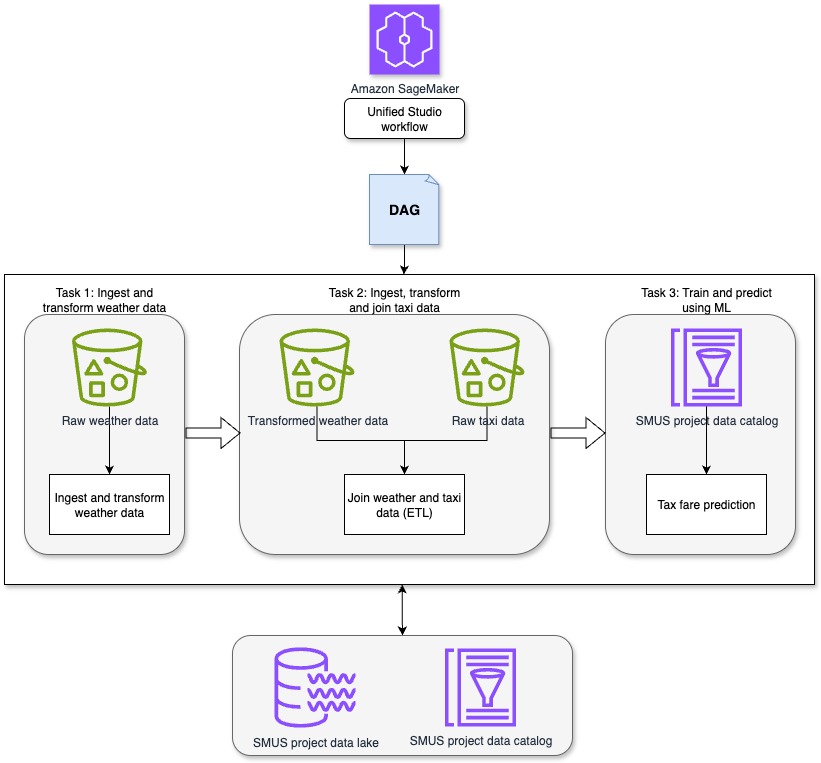
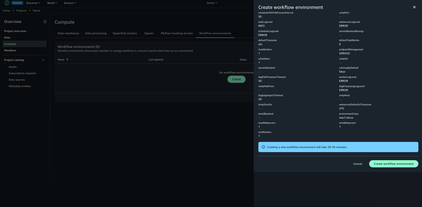
Use Apache Airflow workflows to orchestrate data processing on Amazon SageMaker Unified Studio

Post Syndicated from Vinod Jayendra original https://aws.amazon.com/blogs/big-data/use-apache-airflow-workflows-to-orchestrate-data-processing-on-amazon-sagemaker-unified-studio/

Orchestrating machine learning pipelines is complex, especially when data processing, training, and deployment span multiple services and tools. In this post, we walk through a hands-on, end-to-end example of developing, testing, and running a machine learning (ML) pipeline using workflow capabilities in Amazon SageMaker, accessed through the Amazon SageMaker Unified Studio experience. These workflows are powered by Amazon Managed Workflows for Apache Airflow (Amazon MWAA).

While SageMaker Unified Studio includes a visual builder for low-code workflow creation, this guide focuses on the code-first experience: authoring and managing workflows as Python-based Apache Airflow DAGs (Directed Acyclic Graphs). A DAG is a set of tasks with defined dependencies, where each task runs only after its upstream dependencies are complete, promoting correct execution order and making your ML pipeline more reproducible and resilient.We’ll walk through an example pipeline that ingests weather and taxi data, transforms and joins datasets, and uses ML to predict taxi fares—all orchestrated using SageMaker Unified Studio workflows.

If you prefer a simpler, low-code experience, see Orchestrate data processing jobs, querybooks, and notebooks using visual workflow experience in Amazon SageMaker.

Solution overview

This solution demonstrates how SageMaker Unified Studio workflows can be used to orchestrate a complete data-to-ML pipeline in a centralized environment. The pipeline runs through the following sequential tasks, as shown in the preceding diagram.

  • Task 1: Ingest and transform weather data: This task uses a Jupyter notebook in SageMaker Unified Studio to ingest and preprocess synthetic weather data. The synthetic weather dataset includes hourly observations with attributes such as time, temperature, precipitation, and cloud cover. For this task, the focus is on time, temperature, rain, precipitation, and wind speed.
  • Task 2: Ingest, transform and join taxi data: A second Jupyter notebook in SageMaker Unified Studio ingests the raw New York City taxi ride dataset. This dataset includes attributes such as pickup time, drop-off time, trip distance, passenger count, and fare amount. The relevant fields for this task include pickup and drop-off time, trip distance, number of passengers, and total fare amount. The notebook transforms the taxi dataset in preparation for joining it with the weather data. After transformation, the taxi and weather datasets are joined to create a unified dataset, which is then written to Amazon S3 for downstream use.
  • Task 3: Train and predict using ML: A third Jupyter notebook in SageMaker Unified Studio applies regression techniques to the joined dataset to create a model to determine how attributes of the weather and taxi data such as rain and trip distance impact taxi fares and create a fare prediction model. The trained model is then used to generate fare predictions for new trip data.

This unified approach enables orchestration of extract, transform, and load (ETL) and ML steps with full visibility into the data lifecycle and reproducibility through governed workflows in SageMaker Unified Studio.

Prerequisites

Before you begin, complete the following steps:

  1. Create a SageMaker Unified Studio domain: Follow the instructions in Create an Amazon SageMaker Unified Studio domain – quick setup
  2. Sign in to your SageMaker Unified Studio domain: Use the domain you created in Step 1 sign in. For more information, see Access Amazon SageMaker Unified Studio.
  3. Create a SageMaker Unified Studio project: Create a new project in your domain by following the project creation guide. For Project profile, select All capabilities.

Set up workflows

You can use workflows in SageMaker Unified Studio to set up and run a series of tasks using Apache Airflow to design data processing procedures and orchestrate your querybooks, notebooks, and jobs. You can create workflows in Python code, test and share them with your team, and access the Airflow UI directly from SageMaker Unified Studio. It provides features to view workflow details, including run results, task completions, and parameters. You can run workflows with default or custom parameters and monitor their progress. Now that you have your SageMaker Unified Studio project set up, you can build your workflows.

  1. In your SageMaker Unified Studio project, navigate to the Compute section and select Workflow environment.
  2. Choose Create environment to set up a new workflow environment.
  3. Review the options and choose Create environment. By default, SageMaker Unified Studio creates an mw1.micro class environment, which is suitable for testing and small-scale workflows. To update the environment class before project creation, navigate to Domain and select Project Profiles and then All Capabilities and go to OnDemand Workflows blueprint deployment settings. By using these settings, you can override default parameters and tailor the environment to your specific project requirements.

Develop workflows

You can use workflows to orchestrate notebooks, querybooks, and more in your project repositories. With workflows, you can define a collection of tasks organized as a DAG that can run on a user-defined schedule.To get started:

  1. Download Weather Data Ingestion, Taxi Ingest and Join to Weather, and Prediction notebooks to your local environment.
  2. Go to Build and select JupyterLab; choose Upload files and import the three notebooks you downloaded in the previous step.

  1. Configure your SageMaker Unified Studio space: Spaces are used to manage the storage and resource needs of the relevant application. For this demo, configure the space with an ml.m5.8xlarge instance
    1. Choose Configure Space in the right-hand corner and stop the space.
    2. Update instance type to ml.m5.8xlarge and start the space. Any active processes will be paused during the restart, and any unsaved changes will be lost. Updating the workspace might take a take few minutes.
  2. Go to Build and select Orchestration and then Workflows.
  3. Select the down arrow (▼) next to Create new workflow. From the dropdown menu that appears, select Create in code editor.
  4. In the editor, create a new Python file named multinotebook_dag.py under src/workflows/dags. Copy the following DAG code, which implements a sequential ML pipeline that orchestrates multiple notebooks in SageMaker Unified Studio. Replace <REPLACE-OWNER> with your username. Update NOTEBOOK_PATHS to match your actual notebook locations.
from airflow.decorators import dag
from airflow.utils.dates import days_ago
from workflows.airflow.providers.amazon.aws.operators.sagemaker_workflows import NotebookOperator

WORKFLOW_SCHEDULE = '@daily'

NOTEBOOK_PATHS = [
'<REPLACE FULL PATH FOR Weather_Data_Ingestion.ipynb>',
'<REPLACE FULL PATH FOR Taxi_Weather_Data_Collection.ipynb>',
'<REPLACE FULL PATH FOR Prediction.ipynb>'
]

default_args = {
    'owner': '<REPLACE-OWNER>',
}

@dag(
    dag_id='workflow-multinotebooks',
    default_args=default_args,
    schedule_interval=WORKFLOW_SCHEDULE,
    start_date=days_ago(2),
    is_paused_upon_creation=False,
    tags=['MLPipeline'],
    catchup=False
)
def multi_notebook():
    previous_task = None

    for idx, notebook_path in enumerate(NOTEBOOK_PATHS, 1):
        current_task = NotebookOperator(
            task_id=f"Notebook{idx}task",
            input_config={'input_path': notebook_path, 'input_params': {}},
            output_config={'output_formats': ['NOTEBOOK']},
            wait_for_completion=True,
            poll_interval=5
        )

        # Ensure tasks run sequentially
        if previous_task:
            previous_task >> current_task

        previous_task = current_task  # Update previous task

multi_notebook()

The code uses the NotebookOperator to execute three notebooks in order: data ingestion for weather data, data ingestion for taxi data, and the trained model created by combining the weather and taxi data. Each notebook runs as a separate task, with dependencies to help ensure that they execute in sequence. You can customize with your own notebooks. You can modify the NOTEBOOK_PATHS list to orchestrate any number of notebooks in their workflow while maintaining sequential execution order.

The workflow schedule can be customized by updating WORKFLOW_SCHEDULE (for example: '@hourly', '@weekly', or cron expressions like ‘13 2 1 * *’) to match your specific business needs.

  1. After a workflow environment has been created by a project owner, and once you’ve saved your workflows DAG files in JupyterLab, they are automatically synced to the project. After the files are synced, all project members can view the workflows you have added in the workflow environment. See Share a code workflow with other project members in an Amazon SageMaker Unified Studio workflow environment.

Test and monitor workflow execution

  1. To validate your DAG, Go to Build > Orchestration > Workflows. You should now see the workflow running in Local Space based on the Schedule.

  1. Once the execution completes, workflow would change to success start as shown below.

  1. For each execution, you can zoom in to get a detailed workflow run details and task logs

  1. Access the airflow UI from actions for more information on the dag and execution.

Results

The model’s output is written to the Amazon Simple Storage Service (Amazon S3) output folder as shown the following figure. These results should be evaluated for correctness of fit, prediction accuracy, and the consistency of relationships between variables. If any results appear unexpected or unclear, it is important to review the data, engineering steps, and model assumptions to verify that they align with the intended use case.

Clean up

To avoid incurring additional charges associated with resources created as part of this post, make sure you delete the items created in the AWS account for this post.

  1. The SageMaker domain
  2. The S3 bucket associated with the SageMaker domain

Conclusion

In this post, we demonstrated how you can use Amazon SageMaker to build powerful, integrated ML workflows that span the full data and AI/ML lifecycle. You learned how to create an Amazon SageMaker Unified Studio project, use a multi-compute notebook to process data, and use the built-in SQL editor to explore and visualize results. Finally, we showed you how to orchestrate the entire workflow within the SageMaker Unified Studio interface.

SageMaker offers a comprehensive set of capabilities for data practitioners to perform end-to-end tasks, including data preparation, model training, and generative AI application development. When accessed through SageMaker Unified Studio, these capabilities come together in a single, centralized workspace that helps eliminate the friction of siloed tools, services, and artifacts.

As organizations build increasingly complex, data-driven applications, teams can use SageMaker, together with SageMaker Unified Studio, to collaborate more effectively and operationalize their AI/ML assets with confidence. You can discover your data, build models, and orchestrate workflows in a single, governed environment.

To learn more, visit the Amazon SageMaker Unified Studio page.


About the authors

Suba Palanisamy

Suba Palanisamy

Suba is a Enterprise Support Lead, helping customers achieve operational excellence on AWS. Suba is passionate about all things data and analytics. She enjoys traveling with her family and playing board games.

Sean Bjurstrom

Sean Bjurstrom

Sean is a Enterprise Support Lead in ISV accounts at Amazon Web Services, where he specializes in Analytics technologies and draws on his background in consulting to support customers on their analytics and cloud journeys. Sean is passionate about helping businesses harness the power of data to drive innovation and growth. Outside of work, he enjoys running and has participated in several marathons.

Vinod Jayendra

Vinod Jayendra

Vinod is a Enterprise Support Lead in ISV accounts at Amazon Web Services, where he helps customers in solving their architectural, operational, and cost optimization challenges. With a particular focus on Serverless & Analytics technologies, he draws from his extensive background in application development to deliver top-tier solutions. Beyond work, he finds joy in quality family time, embarking on biking adventures, and coaching youth sports team.

Kamen Sharlandjiev

Kamen Sharlandjiev

Kamen is a Senior Worldwide Specialist SA, Big Data expert. He’s on a mission to make life easier for customers who are facing complex data integration and orchestration challenges. His secret weapon? Fully managed AWS services that can get the job done with minimal effort. Follow Kamen on LinkedIn to keep up to date with the latest MWAA and AWS Glue features and news!

Build data pipelines with dbt in Amazon Redshift using Amazon MWAA and Cosmos

Post Syndicated from Cindy Li original https://aws.amazon.com/blogs/big-data/build-data-pipelines-with-dbt-in-amazon-redshift-using-amazon-mwaa-and-cosmos/

Effective collaboration and scalability are essential for building efficient data pipelines. However, data modeling teams often face challenges with complex extract, transform, and load (ETL) tools, requiring programming expertise and a deep understanding of infrastructure. This complexity can lead to operational inefficiencies and challenges in maintaining data quality at scale.

dbt addresses these challenges by providing a simpler approach where data teams can build robust data models using SQL, a language they’re already familiar with. When integrated with modern development practices, dbt projects can use version control for collaboration, incorporate testing for data quality, and utilize reusable components through macros. dbt also automatically manages dependencies, making sure data transformations execute in the correct sequence.

In this post, we explore a streamlined, configuration-driven approach to orchestrate dbt Core jobs using Amazon Managed Workflows for Apache Airflow (Amazon MWAA) and Cosmos, an open source package. These jobs run transformations on Amazon Redshift, a fully managed data warehouse that enables fast, scalable analytics using standard SQL. With this setup, teams can collaborate effectively while maintaining data quality, operational efficiency, and observability. Key steps covered include:

  • Creating a sample dbt project
  • Enabling auditing within the dbt project to capture runtime metrics for each model
  • Creating a GitHub Actions workflow to automate deployments
  • Setting up Amazon Simple Notification Service (Amazon SNS) to proactively alert on failures

These enhancements enable model-level auditing, automated deployments, and real-time failure alerts. By the end of this post, you will have a practical and scalable framework for running dbt Core jobs with Cosmos on Amazon MWAA, so your team can ship reliable data workflows faster.

Solution overview

The following diagram illustrates the solution architecture.

The workflow contains the following steps:

  1. Analytics engineers manage their dbt project in their version control tool. In this post, we use GitHub as an example.
  2. We configure an Apache Airflow Directed Acyclic Graph (DAG) to use the Cosmos library to create an Airflow task group that contains all the dbt models as part of the dbt project.
  3. We use a GitHub Actions workflow to sync the dbt project files and the DAG to an Amazon Simple Storage Service (Amazon S3) bucket.
  4. During the DAG run, dbt converts the models, tests, and macros to Amazon Redshift SQL statements, which run directly on the Redshift cluster.
  5. If a task in the DAG fails, the DAG invokes an AWS Lambda function to send out a notification using Amazon SNS.

Prerequisites

You must have the following prerequisites:

Create a dbt project

A dbt project is structured to facilitate modular, scalable, and maintainable data transformations. The following code is a sample dbt project structure that this post will follow:

MY_SAMPLE_DBT_PROJECT
├── .github
│   └── workflows
│       └── publish_assets.yml
└── src
    ├── dags
    │   └── dbt_sample_dag.py
    └── my_sample_dbt_project
        ├── macros
        ├── models
        └── dbt_project.yml

dbt uses the following YAML files:

  • dbt_project.yml –  Serves as the main configuration for your project. Objects in this project will inherit settings defined here unless overridden at the model level. For example:
# Name your project! Project names should contain only lowercase characters
# and underscores. 
name: 'my_sample_dbt_project'
version: '1.0.0'

# These configurations specify where dbt should look for different types of files.
# The `model-paths` config, for example, states that models in this project can be
# found in the "models/" directory. 
model-paths: ["models"]
macro-paths: ["macros"]

# Configuring models
# Full documentation: https://docs.getdbt.com/docs/configuring-models
# In this example config, we tell dbt to build models in the example/
# directory as views. These settings can be overridden in the individual model
# files using the `{{ config(...) }}` macro.
models:
  my_sample_dbt_project:
    # Config indicated by + and applies to files under models/example/
    example:
      +materialized: view
      
on-run-end:
# add run results to audit table 
  - "{{ log_audit_table(results) }}" 
  • sources.yml – Defines the external data sources that your dbt models will reference. For example:
sources:
  - name: sample_source
    database: sample_database
    schema: sample_schema
    tables:
      - name: sample_table
  • schema.yml – Outlines the schema of your models and data quality tests. In the following example, we have defined two columns, full_name for the model model1 and sales_id for model2. We have declared them as the primary key and defined data quality tests to check if the two columns are unique and not null.
version: 2

models:
  - name: model1
    config: 
      contract: {enforced: true}

    columns:
      - name: full_name
        data_type: varchar(100)
        constraints:
          - type: primary_key
        tests:
          - unique
          - not_null

  - name: model2
    config: 
      contract: {enforced: true}

    columns:
      - name: sales_id
        data_type: varchar(100)
        constraints:
          - type: primary_key
        tests:
          - unique
          - not_null

Enable auditing within dbt project

Enabling auditing within your dbt project is crucial for facilitating transparency, traceability, and operational oversight across your data pipeline. You can capture run metrics at the model level for each execution in an audit table. By capturing detailed run metrics such as load identifier, runtime, and number of rows affected, teams can systematically monitor the health and performance of each load, quickly identify issues, and trace changes back to specific runs.

The audit table consists of the following attributes:

  • load_id – An identifier for each model run executed as part of the load
  • database_name – The name of the database within which data is being loaded
  • schema_name – The name of the schema within which data is being loaded
  • name – The name of the object within which data is being loaded
  • resource_type – The type of object to which data is being loaded
  • execution_time – The time duration taken for each dbt model to complete execution as part of each load
  • rows_affected – The number of rows affected in the dbt model as part of the load

Complete the following steps to enable auditing within your dbt project:

  1. Navigate to the models directory (src/my_sample_dbt_project/models) and create the audit_table.sql model file:
{%- set run_date = "CURRENT_DATE" -%}
{{
    config(
        materialized='incremental',
        incremental_strategy='append',
        tags=["audit"]
    )
}}

with empty_table as (
    select
        'test_load_id'::varchar(200) as load_id,
        'test_invocation_id'::varchar(200) as invocation_id,
        'test_database_name'::varchar(200) as database_name,
        'test_schema_name'::varchar(200) as schema_name,
        'test_model_name'::varchar(200) as name,
        'test_resource_type'::varchar(200) as resource_type,
        'test_status'::varchar(200) as status,
        cast('12122012' as float) as execution_time,
        cast('100' as int) as rows_affected,
        {{run_date}} as model_execution_date
)

select * from empty_table
-- This is a filter so we will never actually insert these values
where 1 = 0
  1. Navigate to the macros directory (src/my_sample_dbt_project/macros) and create the parse_dbt_results.sql macro file:
{% macro parse_dbt_results(results) %}
    -- Create a list of parsed results
    {%- set parsed_results = [] %}
    -- Flatten results and add to list
    {% for run_result in results %}
        -- Convert the run result object to a simple dictionary
        {% set run_result_dict = run_result.to_dict() %}
        -- Get the underlying dbt graph node that was executed
        {% set node = run_result_dict.get('node') %}
        {% set rows_affected = run_result_dict.get(
        'adapter_response', {}).get('rows_affected', 0) %}
        {%- if not rows_affected -%}
            {% set rows_affected = 0 %}
        {%- endif -%}
        {% set parsed_result_dict = {
                'load_id': invocation_id ~ '.' ~ node.get('unique_id'),
                'invocation_id': invocation_id,
                'database_name': node.get('database'),
                'schema_name': node.get('schema'),
                'name': node.get('name'),
                'resource_type': node.get('resource_type'),
                'status': run_result_dict.get('status'),
                'execution_time': run_result_dict.get('execution_time'),
                'rows_affected': rows_affected
                }%}
        {% do parsed_results.append(parsed_result_dict) %}
    {% endfor %}
    {{ return(parsed_results) }}
{% endmacro %}
  1. Navigate to the macros directory (src/my_sample_dbt_project/macros) and create the log_audit_table.sql macro file:
{% macro log_audit_table(results) %}
    -- depends_on: {{ ref('audit_table') }}
    {%- if execute -%}
        {{ print("Running log_audit_table Macro") }}
        {%- set run_date = "CURRENT_DATE" -%}
        {%- set parsed_results = parse_dbt_results(results) -%}
        {%- if parsed_results | length  > 0 -%}
            {% set allowed_columns = ['load_id', 'invocation_id', 'database_name', 
            'schema_name', 'name', 'resource_type', 'status', 'execution_time', 
            'rows_affected', 'model_execution_date'] -%}
            {% set insert_dbt_results_query -%}
                insert into {{ ref('audit_table') }}
                    (
                        load_id,
                        invocation_id,
                        database_name,
                        schema_name,
                        name,
                        resource_type,
                        status,
                        execution_time,
                        rows_affected,
                        model_execution_date
                ) values
                    {%- for parsed_result_dict in parsed_results -%}
                        (
                            {%- for column, value in parsed_result_dict.items() %}
                                {% if column not in allowed_columns %}
                                    {{ exceptions.raise_compiler_error("Invalid
                                     column") }}
                                {% endif %}
                                {% set sanitized_value = value | replace("'", "''") %}
                                '{{ sanitized_value }}'
                                {%- if not loop.last %}, {% endif %}
                            {%- endfor -%}
                        )
                        {%- if not loop.last %}, {% endif %}
                    {%- endfor -%}
            {%- endset -%}
            {%- do run_query(insert_dbt_results_query) -%}
        {%- endif -%}
    {%- endif -%}
    {{ return ('') }}
{% endmacro %}
  1. Append the following lines to the dbt_project.yml file:
on-run-end:
  - "{{ log_audit_table(results) }}" 

Create a GitHub Actions workflow

This step is optional. If you prefer, you can skip it and instead upload your files directly to your S3 bucket.

The following GitHub Actions workflow automates the deployment of dbt project files and DAG file to Amazon S3. Replace the placeholders {s3_bucket_name}, {account_id}, {role_name}, and {region} with your S3 bucket name, account ID, IAM role name, and AWS Region in the workflow file.

To enhance security, it’s recommended to use OpenID Connect (OIDC) for authentication with IAM roles in GitHub Actions instead of relying on long-lived access keys.

name: Sync dbt Project with S3

on:
  workflow_dispatch:
  push:
    branches: [ main ]
    paths:
      - "src/**"

permissions:
  id-token: write   # This is required for requesting the JWT
  contents: read    # This is required for actions/checkout
  pull-requests: write

jobs:
  sync-dev:
    runs-on: ubuntu-latest
    environment: dev
    defaults:
      run:
        shell: bash
    steps:
      - uses: actions/checkout@v4
      - name: Assume AWS IAM Role
        uses: aws-actions/[email protected]
        with:
          aws-region: {region}
          role-to-assume: arn:aws:iam::{account_id}:role/{role_name}
          role-session-name: my_sample_dbt_project_${{ github.run_id }}
          role-duration-seconds: 3600 # 1 hour

      - run: aws sts get-caller-identity

      - name: Sync dbt Model files
        id: dbt_project_files
        working-directory: src/my_sample_dbt_project
        run: aws s3 sync . s3://{s3_bucket_name}/dags/dbt/my_sample_dbt_project 
        --delete
        continue-on-error: false

      - name: Sync DAG files
        id: dag_file
        working-directory: src/dags
        run: aws s3 sync . s3://{s3_bucket_name}/dags

GitHub has the following security requirements:

  • Branch protection rules – Before proceeding with the GitHub Actions workflow, make sure branch protection rules are in place. These rules enforce required status checks before merging code into protected branches (such as main).
  • Code review guidelines – Implement code review processes to make sure changes undergo review. This can include requiring at least one approving review before code is merged into the protected branch.
  • Incorporate security scanning tools – This can help detect vulnerabilities in your repository.

Make sure you are also adhering to dbt-specific security best practices:

  • Pay attention to dbt macros with variables and validate their inputs.
  • When adding new packages to your dbt project, evaluate their security, compatibility, and maintenance status to make sure they don’t introduce vulnerabilities or conflicts into your project.
  • Review dynamically generated SQL to safeguard against issues like SQL injection.

Update the Amazon MWAA instance

Complete the following steps to update the Amazon MWAA instance:

  1. Install the Cosmos library on Amazon MWAA by adding astronomer-cosmos in the requirements.txt file. Make sure to check for version compatibility for Amazon MWAA and the Cosmos library.
  2. Add the following entries in your startup.sh script:
    1. In the following code, DBT_VENV_PATH specifies the location where the Python virtual environment for dbt will be created. DBT_PROJECT_PATH points to the location of your dbt project inside Amazon MWAA.
      #!/bin/sh
      export DBT_VENV_PATH="${AIRFLOW_HOME}/dbt_venv"
      export DBT_PROJECT_PATH="${AIRFLOW_HOME}/dags/dbt"

    2. The following code creates a Python virtual environment at the path ${DBT_VENV_PATH} and installs the dbt-redshift adapter to run dbt transformations on Amazon Redshift:
      python3 -m venv "${DBT_VENV_PATH}"
      ${DBT_VENV_PATH}/bin/pip install dbt-redshift

Create a dbt user in Amazon Redshift and store credentials

To create dbt models in Amazon Redshift, you must set up a native Redshift user with the necessary permissions to access source tables and create new tables. It is essential to create separate database users with minimal permissions to follow the principle of least privilege. The dbt user should not be granted admin privileges, instead, it should only have access to the specific schemas required for its tasks.

Complete the following steps:

  1. Open the Amazon Redshift console and connect as an admin (for more details, refer to Connecting to an Amazon Redshift database).
  2. Run the following command in the query editor v2 to create a native user, and note down the values for dbt_user_name and password_value:
    create user {dbt_user_name} password 'sha256|{password_value}';

  3. Run the following commands in the query editor v2 to grant permissions to the native user:
    1. Connect to the database where you want to source tables from and run the following commands:
      grant usage on schema {schema_name} to {dbt_user_name};
      grant select on all tables in schema {schema_name} to {dbt_user_name};

    2. To allow the user to create tables within a schema, run the following command:
      grant create on schema {schema_name} to {dbt_user_name};

  4. Optionally, create a secret in AWS Secrets Manager and store the values for dbt_user_name and password_value from the previous step as plaintext:
{
    "username":"dbt_user_name",
    "password":"password_value"
}

Creating a Secrets Manager entry is optional, but recommended for securely storing your credentials instead of hardcoding them. To learn more, refer to AWS Secrets Manager best practices.

Create a Redshift connection in Amazon MWAA

We create one Redshift connection in Amazon MWAA for each Redshift database, making sure that each data pipeline (DAG) can only access one database. This approach provides distinct access controls for each pipeline, helping prevent unauthorized access to data. Complete the following steps:

  1. Log in to the Amazon MWAA UI.
  2. On the Admin menu, choose Connections.
  3. Choose Add a new record.
  4. For Connection Id, enter a name for this connection.
  5. For Connection Type, choose Amazon Redshift.
  6. For Host, enter the endpoint of the Redshift cluster without the port and database name (for example, redshift-cluster-1.xxxxxx.us-east-1.redshift.amazonaws.com).
  7. For Database, enter the database of the Redshift cluster.
  8. For Port, enter the port of the Redshift cluster.

Set up an SNS notification

Setting up SNS notifications is optional, but they can be a useful enhancement to receive alerts on failures. Complete the following steps:

  1. Create an SNS topic.
  2. Create a subscription to the SNS topic.
  3. Create a Lambda function with the Python runtime.
  4. Modify the function code in your Lambda function, and replace {topic_arn} with your SNS topic Amazon Resource Name (ARN):
import json

sns_client = boto3.client('sns')

def lambda_handler(event, context):
     try:
        # Extract DAG name from event
        failed_dag = event['dag_name']
        
        # Send notification 
        sns_client.publish(
            TopicArn={topic_arn}, 
            Subject="Data modelling dags - WARNING", 
            Message=json.dumps({'default': json.dumps(f"Data modelling DAG - 
            {failed_dag} has failed, please inform the data modelling team")}),
            MessageStructure='json'
        )
        
    except KeyError as e:
        # Handle missing 'dag_name' in the event
        logger.error(f"KeyError: invalid payload - dag_name not present")

Configure a DAG

The following sample DAG orchestrates a dbt workflow for processing and auditing data models in Amazon Redshift. It retrieves credentials from Secrets Manager, runs dbt tasks in a virtual environment, and sends an SNS notification if a failure occurs. The workflow consists of the following steps:

  1. It starts with the audit_dbt_task task group, which creates the audit model.
  2. The transform_data task group executes the other dbt models, excluding the audit-tagged one. Inside the transform_data group, there are two dbt models, model1 and model2, and each is followed by a corresponding test task that runs data quality tests defined in the schema.yml file.
  3. To properly detect and handle failures, the DAG includes a dbt_check Python task that runs a custom function, check_dbt_failures. This is important because when using DbtTaskGroup, individual model-level failures inside the group don’t automatically propagate to the task group level. As a result, downstream tasks (such as the Lambda operator sns_notification_for_failure) configured with trigger_rule='one_failed' will not be triggered unless a failure is explicitly raised.

The check_dbt_failures function addresses this by inspecting the results of each dbt model and test, and raising an AirflowException if a failure is found. When an AirflowException is raised, the sns_notification_for_failure task is triggered.

  1. If a failure occurs, the sns_notification_for_failure task invokes a Lambda function to send an SNS notification. If no failures are detected, this task is skipped.

The following diagram illustrates this workflow.

Configure DAG variables

To customize this DAG for your environment, configure the following variables:

  • project_name – Make sure the project_name matches the S3 prefix of your dbt project
  • secret_name – Provide the name of the secret that stores dbt user credentials
  • target_database and target_schema – Update these variables to reflect where you want to land your dbt models in Amazon Redshift
  • redshift_connection_id – Set this to match the connection configured in Amazon MWAA for this Redshift database
  • sns_lambda_function_name – Provide the Lambda function name to send SNS notifications
  • dag_name – Provide the DAG name that will be passed to the SNS notification Lambda function
import os
import json
import boto3
from airflow import DAG
from cosmos import (
    DbtTaskGroup, ProfileConfig, ProjectConfig,
    ExecutionConfig, RenderConfig
)
from cosmos.constants import ExecutionMode, LoadMode
from cosmos.profiles import RedshiftUserPasswordProfileMapping
from pendulum import datetime
from airflow.operators.python_operator import PythonOperator
from airflow.providers.amazon.aws.operators.lambda_function import (
    LambdaInvokeFunctionOperator
)
from airflow.exceptions import AirflowException

# project name - should match the s3 prefix of your dbt project
project_name = "my_sample_dbt_project"
# name of the secret that stores dbt user credentials 
secret_name = "dbt_user_credentials_secret"
# target database to land dbt models
target_database = "sample_database"
# target schema to land dbt models
target_schema = "sample_schema"
# Redshift connection name from MWAA
redshift_connection_id = "my_sample_dbt_project_connection"
# sns lambda function name
sns_lambda_function_name = "sns_notification"
# dag name - this will be passed to SNS for notification
payload = json.dumps({
            "dag_name": "my_sample_dbt_project_dag"
        })

Incorporate DAG components

After setting the variables, you can now incorporate the following components to complete the DAG.

Secrets Manager

The DAG retrieves dbt user credentials from Secrets Manager:

sm_client = boto3.client('secretsmanager')

def get_secret(secret_name):
    try:
        get_secret_value_response = sm_client.get_secret_value(SecretId=secret_name)
        return json.loads(get_secret_value_response["SecretString"])
    except Exception as e:
        raise

secret_value = get_secret(secret_name)
username = secret_value["username"]
password = secret_value["password"]

Redshift connection configuration

It uses RedshiftUserPasswordProfileMapping to authenticate:

profile_config = ProfileConfig(
    profile_name="redshift",
    target_name=target_database,
    profile_mapping=RedshiftUserPasswordProfileMapping(
        conn_id=redshift_connection_id,
        profile_args={"schema": target_schema,
                      "user": username, "password": password}
    ),
)

dbt execution setup

This code contains the following variables:

  • dbt executable path – Uses a virtual environment
  • dbt project path – Is located in the environment variable DBT_PROJECT_PATH under your project
execution_config = ExecutionConfig(
    dbt_executable_path=f"{os.environ['DBT_VENV_PATH']}/bin/dbt",
    execution_mode=ExecutionMode.VIRTUALENV,
)

project_config = ProjectConfig(
    dbt_project_path=f"{os.environ['DBT_PROJECT_PATH']}/{project_name}",
)

Tasks and execution flow

This step includes the following components:

  • Audit dbt task group (audit_dbt_task) – Runs the dbt model tagged with audit
  • dbt task group (transform_data) – Runs the dbt models tagged with operations, excluding the audit model

In dbt, tags are labels that you can assign to models, tests, seeds, and other dbt resources to organize and selectively run subsets of your dbt project. In your render_config, you have exclude=["tag:audit"]. This means dbt will exclude models that have the tag audit, because the audit model runs separately.

  • Failure check (dbt_check) – Checks for dbt model failures, raises an AirflowException if upstream dbt tasks fail
  • SNS notification on failure (sns_notification_for_failure) – Invokes a Lambda function to send an SNS notification upon a dbt task failure (for example, a dbt model in the task group)
def check_dbt_failures(**kwargs):
    if kwargs['ti'].state == 'failed':
        raise AirflowException('Failure in dbt task group')

with DAG(
    dag_id="my_sample_dbt_project_dag",
    start_date=datetime(2025, 4, 2),
    schedule_interval="@daily",
    catchup=False,
    tags=["dbt"]
):

    audit_dbt_task = DbtTaskGroup(
        group_id="audit_dbt_task",
        execution_config=execution_config,
        profile_config=profile_config,
        project_config=project_config,
        operator_args={
            "install_deps": True,
        },
        render_config= RenderConfig(
            select=["tag:audit"],
            load_method=LoadMode.DBT_LS
        )
    )

    transform_data = DbtTaskGroup(
        group_id="transform_data",
        execution_config=execution_config,
        profile_config=profile_config,
        project_config=project_config,
        operator_args={
            "install_deps": True,
            # install necessary dependencies before running dbt command
        },
        render_config= RenderConfig(
            exclude=["tag:audit"],
            load_method=LoadMode.DBT_LS
        )
    )

    dbt_check = PythonOperator(
        task_id='dbt_check', 
        python_callable=check_dbt_failures,
        provide_context=True,
    )

    sns_notification_for_failure = LambdaInvokeFunctionOperator(
        task_id="sns_notification_for_failure",
        function_name=sns_lambda_function_name,
        payload=payload,
        trigger_rule='one_failed'
    )

    audit_dbt_task >> transform_data >> dbt_check >> sns_notification_for_failure

The sample dbt orchestrates a dbt workflow in Amazon Redshift, starting with an audit task and followed by a task group that processes data models. It includes a failure handling mechanism that checks for failures and raises an exception to trigger an SNS notification using Lambda if a failure occurs. If no failures are detected, the SNS notification task is skipped.

Clean up

If you no longer need the resources you created, delete them to avoid additional charges. This includes the following:

  • Amazon MWAA environment
  • S3 bucket
  • IAM role
  • Redshift cluster or serverless workgroup
  • Secrets Manager secret
  • SNS topic
  • Lambda function

Conclusion

By integrating dbt with Amazon Redshift and orchestrating workflows using Amazon MWAA and the Cosmos library, you can simplify data transformation workflows while maintaining robust engineering practices. The sample dbt project structure, combined with automated deployments through GitHub Actions and proactive monitoring using Amazon SNS, provides a foundation for building reliable data pipelines. The addition of audit logging facilitates transparency across your transformations, so teams can maintain high data quality standards.

You can use this solution as a starting point for your own dbt implementation on Amazon MWAA. The approach we outlined emphasizes SQL-based transformations while incorporating essential operational capabilities like deployment automation and failure alerting. Get started by adapting the configuration to your environment, and build upon these practices as your data needs evolve.

For more resources, refer to Manage data transformations with dbt in Amazon Redshift and Redshift setup.


About the authors

Cindy Li is an Associate Cloud Architect at AWS Professional Services, specialising in Data Analytics. Cindy works with customers to design and implement scalable data analytics solutions on AWS. When Cindy is not diving into tech, you can find her out on walks with her playful toy poodle Mocha.

Akhil B is a Data Analytics Consultant at AWS Professional Services, specializing in cloud-based data solutions. He partners with customers to design and implement scalable data analytics platforms, helping organizations transform their traditional data infrastructure into modern, cloud-based solutions on AWS. His expertise helps organizations optimize their data ecosystems and maximize business value through modern analytics capabilities.

Joao Palma is a Senior Data Architect at Amazon Web Services, where he partners with enterprise customers to design and implement comprehensive data platform solutions. He specializes in helping organizations transform their data into strategic business assets and enabling data-driven decision making.

Harshana Nanayakkara is a Delivery Consultant at AWS Professional Services, where he helps customers tackle complex business challenges using AWS Cloud technology. He specializes in data and analytics, data governance, and AI/ML implementations.

Best practices for upgrading Amazon MWAA environments

Post Syndicated from Anurag Srivastava original https://aws.amazon.com/blogs/big-data/best-practices-for-upgrading-amazon-mwaa-environments/

Amazon Managed Workflows for Apache Airflow (Amazon MWAA) has become a cornerstone for organizations embracing data-driven decision-making. As a scalable solution for managing complex data pipelines, Amazon MWAA enables seamless orchestration across AWS services and on-premises systems. Although AWS manages the underlying infrastructure, you must carefully plan and execute your Amazon MWAA environment updates according to the shared responsibility model. Upgrading to the latest Amazon MWAA version can provide significant advantages, including enhanced security through critical security patches and potential improvements in performance with faster DAG parsing and reduced database load. You can use advanced features while maintaining ecosystem compatibility and receiving prioritized AWS support. The key to successful upgrades lies in choosing the right solution and following a methodical implementation approach.

In this post, we explore best practices for upgrading your Amazon MWAA environment and provide a step-by-step guide to seamlessly transition to the latest version.

Solution overview

Amazon MWAA provides two primary upgrade solutions:

  • In-place upgrade – This method works best when you can accommodate planned downtime. You deploy the new version directly on your existing infrastructure. In-place version upgrades on Amazon MWAA are supported for environments running Apache Airflow version 2.x and later. However, if you’re running version 1.10.z or older versions, you must create a new environment and migrate your resources, because these versions don’t support in-place upgrades.
  • Cutover upgrade – This method helps minimize disruption to production environments. You create a new Amazon MWAA environment with the target version and then transition from your old environment to the new one.

Each solution offers a different approach to help you upgrade while working to maintain data integrity and system reliability.

In-place upgrade

In-place upgrades work well for environments where you can schedule a maintenance window for the upgrade process. During this window, Amazon MWAA preserves your workflow history. This method works best when you can accommodate planned downtime. It helps maintain historical data, provides a straightforward upgrade process, and includes rollback capabilities if issues occur during provisioning. You also use fewer resources because you don’t need to create a new environment.

You can perform in-place upgrades through the AWS Management Console with a single operation. This process helps reduce operational overhead by managing many upgrade steps for you.

During the upgrade process, your environment can’t schedule or run new tasks. Amazon MWAA helps manage the upgrade process and implements safety measures—if issues occur during the provisioning phase, the service attempts to revert to the previous stable version.

Before you begin an in-place upgrade, we recommend testing your DAGs for compatibility with the target version, because DAG compatibility issues can affect the upgrade process. You can use the Amazon MWAA local runner to test DAG compatibility before you start the upgrade. You can start the upgrade using either the console and specifying the new version or the AWS Command Line Interface (AWS CLI). The following is an example Amazon MWAA upgrade command using the AWS CLI:

aws mwaa update-environment --name <value> --airflow-version <value>

The following diagram shows the Amazon MWAA in-place upgrade workflow and states.

In-place upgrade workflow and states

Refer to Introducing in-place version upgrades with Amazon MWAA for more details.

Cutover upgrade

A cutover upgrade provides an alternative solution when you need to minimize downtime, though it requires more manual steps and operational planning. With this approach, you create a new Amazon MWAA environment, migrate your metadata, and manage the transition between environments. Although this method offers more control over the upgrade process, it requires additional planning and execution effort compared to an in-place upgrade.

This method can work well for environments with complex workflows, particularly when you plan to make significant changes alongside the version upgrade. The approach offers several benefits: you can minimize production downtime, perform comprehensive testing before switching environments, and maintain the ability to return to your original environment if needed. You can also review and update your configurations during the transition.

Consider the following aspects of the cutover approach. When you run two environments simultaneously, you pay for both environments. The pricing for each Amazon MWAA environment depends on:

  • Duration of environment uptime (billed hourly with per-second resolution)
  • Environment size configuration
  • Automatic scaling capacity for workers
  • Scheduler capacity

AWS calculates the cost of additional automatic scaled workers separately. You can estimate costs for your specific configuration using the AWS Pricing Calculator.

To help prevent data duplication or corruption during parallel operation, we recommend implementing idempotent DAGs. The Airflow scheduler automatically populates some metadata tables (dag, dag_tag, and dag_code) in your new environment. However, you need to plan the migration of the following additional metadata components:

  • DAG history
  • Variables
  • Slot pool configurations
  • SLA miss records
  • XCom data
  • Job records
  • Log tables

You can choose this approach when your requirements prioritize minimal downtime and you can manage the additional operational complexity.

The cutover upgrade process involves three main steps: creating a new environment, restoring it with the existing data, and performing the upgrade. The following diagram illustrates the full workflow.

Cut-over upgrade steps

In the following sections, we walk through the key steps to perform a cutover upgrade.

Prerequisites

Before you begin the upgrade process, complete the following steps:

Create a new environment

Complete the following steps to create a new environment:

  • Generate a template for your new environment configuration using the AWS CLI:

aws mwaa create-environment --generate-cli-skeleton > <new-env-name>.json

  • Modify the generated JSON file:
    • Copy configurations from your backup file <env-name>.json to <new-env-name>.json.
    • Update the environment name.
    • Keep the AirflowVersion parameter value from your existing environment.
    • Review and update other configuration parameters as needed.
  • Create your new environment:

aws mwaa create-environment --cli-input-json <content of new-env-name.json>

Restore the new environment

Complete the following steps to restore the new environment:

  • Use the mwaa-dr PyPI package to create and run the restore DAG.
  • This process copies metadata from your S3 backup bucket to the new environment.
  • Verify that your new environment contains the expected metadata from your original environment.

Perform the version upgrade

Complete the following steps to perform the version upgrade:

  • Upgrade your environment:

aws mwaa update-environment --name <new-env-name> --airflow-version <target-version>

  • Monitor the upgrade:
    • Track the environment status on the console.
    • Watch for error messages or warnings.
    • Verify the environment reaches the AVAILABLE

Plan your transition timing carefully. When your original environment continues to process workflows during this upgrade, the metadata between environments can change.

Clean up

After you verify the stability of your upgraded environment through monitoring, you can begin the cleanup process:

  • Remove your original Amazon MWAA environment using the AWS CLI command:

 aws mwaa delete-environment --name <old-env-name>

  • Clean up your associated resources by removing unused backup data from S3 buckets, deleting temporary AWS Identity and Access Management (IAM) roles and policies created for the upgrade, and updating your DNS or routing configurations.

Before removing any resources, make sure you follow your organization’s backup retention policies, maintain necessary backup data for your compliance requirements, and document configuration changes made during the upgrade.

This approach helps you perform a controlled upgrade with opportunities for testing and the ability to return to your original environment if needed.

Monitoring and validation

You can track your upgrade progress using Amazon CloudWatch metrics, with a focus on DAG processing metrics and scheduler heartbeat. Your environment transitions through several states during the upgrade process, including UPDATING and CREATING. When your environment shows the AVAILABLE state, you can begin validation testing. We recommend checking system accessibility, testing critical workflow operations, and verifying external connections. For detailed monitoring guidance, see Monitoring and metrics for Amazon Managed Workflows for Apache Airflow.

Key considerations

Consider using infrastructure as code (IaC) practices to help maintain consistent environment management and support repeatable deployments. Schedule metadata backups using mwaa-dr during periods of low activity to help protect your data. When designing your workflows, implement idempotent pipelines to help manage potential interruptions, and maintain documentation of your configurations and dependencies.

Conclusion

A successful Amazon MWAA upgrade starts with selecting an approach that aligns with your operational requirements. Whether you choose an in-place or cutover upgrade, thorough preparation and testing help support a controlled transition. Using available tools, monitoring capabilities, and recommended practices can help you upgrade to the latest Amazon MWAA features while working to maintain your workflow operations.

For additional details and code examples on Amazon MWAA, refer to the Amazon MWAA User Guide and Amazon MWAA examples GitHub repo.

Apache, Apache Airflow, and Airflow are either registered trademarks or trademarks of the Apache Software Foundation in the United States and/or other countries.


About the Authors

Anurag Srivastava works as a Senior Big Data Cloud Engineer at Amazon Web Services (AWS), specializing in Amazon MWAA. He’s passionate about helping customers build scalable data pipelines and workflow automation solutions on AWS.

Sriharsh Adari is a Senior Solutions Architect at Amazon Web Services (AWS), where he helps customers work backwards from business outcomes to develop innovative solutions on AWS. Over the years, he has helped multiple customers on data platform transformations across industry verticals. His core area of expertise include Technology Strategy, Data Analytics, and Data Science. In his spare time, he enjoys playing sports, binge-watching TV shows, and playing Tabla.
Venu Thangalapally is a Senior Solutions Architect at AWS, based in Chicago, with deep expertise in cloud architecture, data and analytics, containers, and application modernization. He partners with Financial Services industry customers to translate business goals into secure, scalable, and compliant cloud solutions that deliver measurable value. Venu is passionate about leveraging technology to drive innovation and operational excellence. Outside of work, he enjoys spending time with his family, reading, and taking long walks.

Chandan Rupakheti is a Senior Solutions Architect at AWS. His main focus at AWS lies in the intersection of analytics, serverless, and AdTech services. He is a passionate technical leader, researcher, and mentor with a knack for building innovative solutions in the cloud. Outside of his professional life, he loves spending time with his family and friends, and listening to and playing music.

How LaunchDarkly migrated to Amazon MWAA to achieve efficiency and scale

Post Syndicated from Asena Uyar, Dean Verhey original https://aws.amazon.com/blogs/big-data/how-launchdarkly-migrated-to-amazon-mwaa-to-achieve-efficiency-and-scale/

This is a guest post coauthored with LaunchDarkly.

The LaunchDarkly feature management platform equips software teams to proactively reduce the risk of shipping bad software and AI applications while accelerating their release velocity. In this post, we explore how LaunchDarkly scaled the internal analytics platform up to 14,000 tasks per day, with minimal increase in costs, after migrating from another vendor-managed Apache Airflow solution to AWS, using Amazon Managed Workflows for Apache Airflow (Amazon MWAA) and Amazon Elastic Container Service (Amazon ECS). We walk you through the issues we ran into during the migration, the technical solution we implemented, the trade-offs we made, and lessons we learned along the way.

The challenge

LaunchDarkly has a mission to enable high-velocity teams to release, monitor, and optimize software in production. The centralized data team is responsible for tracking how LaunchDarkly is progressing toward that mission. Additionally, this team is responsible for the majority of the company’s internal data needs, which include ingesting, warehousing, and reporting on the company’s data. Some of the large datasets we manage include product usage, customer engagement, revenue, and marketing data.

As the company grew, our data volume increased, and the complexity and use cases of our workloads expanded exponentially. While using other vendor-managed Airflow-based solutions, our data analytics team faced new challenges on time to integrate and onboard new AWS services, data locality, and a non-centralized orchestration and monitoring solution across different engineering teams within the organization.

Solution overview

LaunchDarkly has a long history of using AWS services to solve business use cases, such as scaling our ingestion from 1 TB to 100 TB per day with Amazon Kinesis Data Streams. Similarly, migrating to Amazon MWAA helped us scale and optimize our internal extract, transform, and load (ETL) pipelines. We used existing monitoring and infrastructure as code (IaC) implementations and eventually extended Amazon MWAA to other teams, establishing it as a centralized batch processing solution orchestrating multiple AWS services.

The solution for our transformation jobs include the following components:

Our original plan for the Amazon MWAA migration was:

  1. Create a new Amazon MWAA instance using Terraform following LaunchDarkly service standards.
  2. Lift and shift (or rehost) our code base from Airflow 1.12 to Airflow 2.5.1 on the original cloud provider to the same version on Amazon MWAA.
  3. Cut over all Directed Acyclic Graph (DAG) runs to AWS.
  4. Upgrade to Airflow 2.
  5. With the flexibility and ease of integration within AWS ecosystem, iteratively make enhancements around containerization, logging, and continuous deployment.

Steps 1 and 2 were executed quickly—we used the Terraform AWS provider and the existing LaunchDarkly Terraform infrastructure to build a reusable Amazon MWAA module initially at Airflow version 1.12. We had an Amazon MWAA instance and the supporting pieces (CloudWatch and artifacts S3 bucket) running on AWS within a week.

When we started cutting over DAGs to Amazon MWAA in Step 3, we ran into some issues. At the time of migration, our Airflow code base was centered around a custom operator implementation that created a Python virtual environment for our workload requirements on the Airflow worker disk assigned to the task. By trial and error in our migration attempt, we learned that this custom operator was essentially dependent on the behavior and isolation of Airflow’s Kubernetes executors used in the original cloud provider platform. When we began to run our DAGs concurrently on Amazon MWAA (which uses Celery Executor workers that behave differently), we ran into a few transient issues where the behavior of that custom operator could affect other running DAGs.

At this time, we took a step back and evaluated solutions for promoting isolation between our running tasks, eventually landing on Fargate for ECS tasks that could be started from Amazon MWAA. We had initially planned to move our tasks to their own isolated system rather than having them run directly in Airflow’s Python runtime environment. Due to the circumstances, we decided to advance this requirement, transforming our rehosting project into a refactoring migration.

We chose Amazon ECS on Fargate for its ease of use, existing Airflow integrations (ECSRunTaskOperator), low cost, and lower management overhead compared to a Kubernetes-based solution such as Amazon Elastic Kubernetes Service (Amazon EKS). Although a solution using Amazon EKS would improve the task provisioning time even further, the Amazon ECS solution met the latency requirements of the data analytics team’s batch pipelines. This was acceptable because these queries run for several minutes on a periodic basis, so a couple more minutes for spinning up each ECS task didn’t significantly impact overall performance.

Our first Amazon ECS implementation involved a single container that downloads our project from an artifacts repository on Amazon S3, and runs the command passed to the ECS task. We trigger those tasks using the ECSRunTaskOperator in a DAG in Amazon MWAA, and created a wrapper around the built-in Amazon ECS operator, so analysts and engineers on the data analytics team could create new DAGs just by specifying the commands they were already familiar with.

The following diagram illustrates the DAG and task deployment flows.

End-to-end AWS workflow diagram illustrating automated DAGs and Tasks deployment through GitHub, CircleCI, S3, MWAA, and ECS

When our initial Amazon ECS implementation was complete, we were able to cut all of our existing DAGs over to Amazon MWAA without the prior concurrency issues, because each task ran in its own isolated Amazon ECS task on Fargate.

Within a few months, we proceeded to Step 4 to upgrade our Amazon MWAA instance to Airflow 2. This was a major version upgrade (from 1.12 to 2.5.1), which we implemented by following the Amazon MWAA Migration Guide and subsequently tearing down our legacy resources.

The cost increase of adding Amazon ECS to our pipelines was minimal. This was because our pipelines run on batch schedules, and therefore aren’t active at all times, and Amazon ECS on Fargate only charges for vCPU and memory resources requested to complete the tasks.

As a part of Step 5 for continuous assessment and improvements, we enhanced our Amazon ECS implementation to push logs and metrics to Datadog and CloudWatch. We could monitor for errors and model performance, and catch data test failures alongside existing LaunchDarkly monitoring.

Scaling the solution beyond internal analytics

During the initial implementation for the data analytics team, we created an Amazon MWAA Terraform module, which enabled us to quickly spin up more Amazon MWAA environments and share our work with other engineering teams. This allowed the use of Airflow and Amazon MWAA to power batch pipelines within the LaunchDarkly product itself in a couple of months shortly after the data analytics team completed the initial migration.

The numerous AWS service integrations supported by Airflow, the built-in Amazon provider package, and Amazon MWAA allowed us to expand our usage across teams to use Amazon MWAA as a generic orchestrator for distributed pipelines across services like Amazon Athena, Amazon Relational Database Service (Amazon RDS), and AWS Glue. Since adopting the service, onboarding a new AWS service to Amazon MWAA has been straightforward, typically involving the identification of the existing Airflow Operator or Hook to use, and then connecting the two services with AWS Identity and Access Management (IAM).

Lessons and results

Through our journey of orchestrating data pipelines at scale with Amazon MWAA and Amazon ECS, we’ve gained valuable insights and lessons that have shaped the success of our implementation. One of the key lessons learned was the importance of isolation. During the initial migration to Amazon MWAA, we encountered issues with our custom Airflow operator that relied on the specific behavior of the Kubernetes executors used in the original cloud provider platform. This highlighted the need for isolated task execution to maintain the reliability and scalability of our pipelines.

As we scaled our implementation, we also recognized the importance of monitoring and observability. We enhanced our monitoring and observability by integrating with tools like Datadog and CloudWatch, so we could better monitor errors and model performance and catch data test failures, improving the overall reliability and transparency of our data pipelines.

With the previous Airflow implementation, we were running approximately 100 Airflow tasks per day across one team and two services (Amazon ECS and Snowflake). As of the time of writing this post, we’ve scaled our implementation to three teams, four services, and execution of over 14,000 Airflow tasks per day. Amazon MWAA has become a critical component of our batch processing pipelines, increasing the speed of onboarding new teams, services, and pipelines to our data platform from weeks to days.

Looking ahead, we plan to continue iterating on this solution to expand our use of Amazon MWAA to additional AWS services such as AWS Lambda and Amazon Simple Queue Service (Amazon SQS), and further automate our data workflows to support even greater scalability as our company grows.

Conclusion

Effective data orchestration is essential for organizations to gather and unify data from diverse sources into a centralized, usable format for analysis. By automating this process across teams and services, businesses can transform fragmented data into valuable insights to drive better decision-making. LaunchDarkly has achieved this by using managed services like Amazon MWAA and adopting best practices such as task isolation and observability, enabling the company to accelerate innovation, mitigate risks, and shorten the time-to-value of its product offerings.

If your organization is planning to modernize its data pipelines orchestration, start assessing your current workflow management setup, exploring the capabilities of Amazon MWAA, and considering how containerization could benefit your workflows. With the right tools and approach, you can transform your data operations, drive innovation, and stay ahead of growing data processing demands.


About the Authors

Asena Uyar is a Software Engineer at LaunchDarkly, focusing on building impactful experimentation products that empower teams to make better decisions. With a background in mathematics, industrial engineering, and data science, Asena has been working in the tech industry for over a decade. Her experience spans various sectors, including SaaS and logistics, and she has spent a significant portion of her career as a Data Platform Engineer, designing and managing large-scale data systems. Asena is passionate about using technology to simplify and optimize workflows, making a real difference in the way teams operate.

Dean Verhey is a Data Platform Engineer at LaunchDarkly based in Seattle. He’s worked all across data at LaunchDarkly, ranging from internal batch reporting stacks to streaming pipelines powering product features like experimentation and flag usage charts. Prior to LaunchDarkly, he worked in data engineering for a variety of companies, including procurement SaaS, travel startups, and fire/EMS records management. When he’s not working, you can often find him in the mountains skiing.

Daniel Lopes is a Solutions Architect for ISVs at AWS. His focus is on enabling ISVs to design and build their products in alignment with their business goals with all advantages AWS services can provide them. His areas of interest are event-driven architectures, serverless computing, and generative AI. Outside work, Daniel mentors his kids in video games and pop culture.