Post Syndicated from Randy DeFauw original https://aws.amazon.com/blogs/big-data/build-a-rag-data-ingestion-pipeline-for-large-scale-ml-workloads/
For building any generative AI application, enriching the large language models (LLMs) with new data is imperative. This is where the Retrieval Augmented Generation (RAG) technique comes in. RAG is a machine learning (ML) architecture that uses external documents (like Wikipedia) to augment its knowledge and achieve state-of-the-art results on knowledge-intensive tasks. For ingesting these external data sources, Vector databases have evolved, which can store vector embeddings of the data source and allow for similarity searches.
In this post, we show how to build a RAG extract, transform, and load (ETL) ingestion pipeline to ingest large amounts of data into an Amazon OpenSearch Service cluster and use Amazon Relational Database Service (Amazon RDS) for PostgreSQL with the pgvector extension as a vector data store. Each service implements k-nearest neighbor (k-NN) or approximate nearest neighbor (ANN) algorithms and distance metrics to calculate similarity. We introduce the integration of Ray into the RAG contextual document retrieval mechanism. Ray is an open source, Python, general purpose, distributed computing library. It allows distributed data processing to generate and store embeddings for a large amount of data, parallelizing across multiple GPUs. We use a Ray cluster with these GPUs to run parallel ingest and query for each service.
In this experiment, we attempt to analyze the following aspects for OpenSearch Service and the pgvector extension on Amazon RDS:
- As a vector store, the ability to scale and handle a large dataset with tens of millions of records for RAG
- Possible bottlenecks in the ingest pipeline for RAG
- How to achieve optimal performance in ingestion and query retrieval times for OpenSearch Service and Amazon RDS
To understand more about vector data stores and their role in building generative AI applications, refer to The role of vector datastores in generative AI applications.
Overview of OpenSearch Service
OpenSearch Service is a managed service for secure analysis, search, and indexing of business and operational data. OpenSearch Service supports petabyte-scale data with the ability to create multiple indexes on text and vector data. With optimized configuration, it aims for high recall for the queries. OpenSearch Service supports ANN as well as exact k-NN search. OpenSearch Service supports a selection of algorithms from the NMSLIB, FAISS, and Lucene libraries to power the k-NN search. We created the ANN index for OpenSearch with the Hierarchical Navigable Small World (HNSW) algorithm because it’s regarded as a better search method for large datasets. For more information on the choice of index algorithm, refer to Choose the k-NN algorithm for your billion-scale use case with OpenSearch.
Overview of Amazon RDS for PostgreSQL with pgvector
The pgvector extension adds an open source vector similarity search to PostgreSQL. By utilizing the pgvector extension, PostgreSQL can perform similarity searches on vector embeddings, providing businesses with a speedy and proficient solution. pgvector provides two types of vector similarity searches: exact nearest neighbor, which results with 100% recall, and approximate nearest neighbor (ANN), which provides better performance than exact search with a trade-off on recall. For searches over an index, you can choose how many centers to use in the search, with more centers providing better recall with a trade-off of performance.
Solution overview
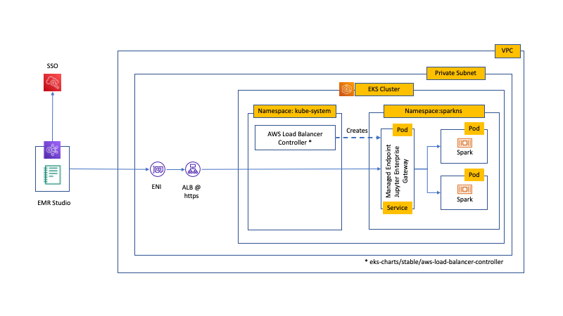
The following diagram illustrates the solution architecture.

Let’s look at the key components in more detail.
Dataset
We use OSCAR data as our corpus and the SQUAD dataset to provide sample questions. These datasets are first converted to Parquet files. Then we use a Ray cluster to convert the Parquet data to embeddings. The created embeddings are ingested to OpenSearch Service and Amazon RDS with pgvector.
OSCAR (Open Super-large Crawled Aggregated corpus) is a huge multilingual corpus obtained by language classification and filtering of the Common Crawl corpus using the ungoliant architecture. Data is distributed by language in both original and deduplicated form. The Oscar Corpus dataset is approximately 609 million records and takes up about 4.5 TB as raw JSONL files. The JSONL files are then converted to Parquet format, which minimizes the total size to 1.8 TB. We further scaled the dataset down to 25 million records to save time during ingestion.
SQuAD (Stanford Question Answering Dataset) is a reading comprehension dataset consisting of questions posed by crowd workers on a set of Wikipedia articles, where the answer to every question is a segment of text, or span, from the corresponding reading passage, or the question might be unanswerable. We use SQUAD, licensed as CC-BY-SA 4.0, to provide sample questions. It has approximately 100,000 questions with over 50,000 unanswerable questions written by crowd workers to look similar to answerable ones.
Ray cluster for ingestion and creating vector embeddings
In our testing, we found that the GPUs make the biggest impact to performance when creating the embeddings. Therefore, we decided to use a Ray cluster to convert our raw text and create the embeddings. Ray is an open source unified compute framework that enables ML engineers and Python developers to scale Python applications and accelerate ML workloads. Our cluster consisted of 5 g4dn.12xlarge Amazon Elastic Compute Cloud (Amazon EC2) instances. Each instance was configured with 4 NVIDIA T4 Tensor Core GPUs, 48 vCPU, and 192 GiB of memory. For our text records, we ended up chunking each into 1,000 pieces with a 100-chunk overlap. This breaks out to approximately 200 per record. For the model used to create embeddings, we settled on all-mpnet-base-v2 to create a 768-dimensional vector space.
Infrastructure setup
We used the following RDS instance types and OpenSearch service cluster configurations to set up our infrastructure.
The following are our RDS instance type properties:
- Instance type: db.r7g.12xlarge
- Allocated storage: 20 TB
- Multi-AZ: True
- Storage encrypted: True
- Enable Performance Insights: True
- Performance Insight retention: 7 days
- Storage type: gp3
- Provisioned IOPS: 64,000
- Index type: IVF
- Number of lists: 5,000
- Distance function: L2
The following are our OpenSearch Service cluster properties:
- Version: 2.5
- Data nodes: 10
- Data node instance type: r6g.4xlarge
- Primary nodes: 3
- Primary node instance type: r6g.xlarge
- Index: HNSW engine:
nmslib - Refresh interval: 30 seconds
ef_construction: 256- m: 16
- Distance function: L2
We used large configurations for both the OpenSearch Service cluster and RDS instances to avoid any performance bottlenecks.
We deploy the solution using an AWS Cloud Development Kit (AWS CDK) stack, as outlined in the following section.
Deploy the AWS CDK stack
The AWS CDK stack allows us to choose OpenSearch Service or Amazon RDS for ingesting data.
Pre-requsities
Before proceeding with the installation, under cdk, bin, src.tc, change the Boolean values for Amazon RDS and OpenSearch Service to either true or false depending on your preference.
You also need a service-linked AWS Identity and Access Management (IAM) role for the OpenSearch Service domain. For more details, refer to Amazon OpenSearch Service Construct Library. You can also run the following command to create the role:
This AWS CDK stack will deploy the following infrastructure:
- A VPC
- A jump host (inside the VPC)
- An OpenSearch Service cluster (if using OpenSearch service for ingestion)
- An RDS instance (if using Amazon RDS for ingestion)
- An AWS Systems Manager document for deploying the Ray cluster
- An Amazon Simple Storage Service (Amazon S3) bucket
- An AWS Glue job for converting the OSCAR dataset JSONL files to Parquet files
- Amazon CloudWatch dashboards
Download the data
Run the following commands from the jump host:
Before cloning the git repo, make sure you have a Hugging Face profile and access to the OSCAR data corpus. You need to use the user name and password for cloning the OSCAR data:
Convert JSONL files to Parquet
The AWS CDK stack created the AWS Glue ETL job oscar-jsonl-parquet to convert the OSCAR data from JSONL to Parquet format.
After you run the oscar-jsonl-parquet job, the files in Parquet format should be available under the parquet folder in the S3 bucket.
Download the questions
From your jump host, download the questions data and upload it to your S3 bucket:
Set up the Ray cluster
As part of the AWS CDK stack deployment, we created a Systems Manager document called CreateRayCluster.
To run the document, complete the following steps:
- On the Systems Manager console, under Documents in the navigation pane, choose Owned by Me.
- Open the
CreateRayClusterdocument. - Choose Run.
The run command page will have the default values populated for the cluster.
The default configuration requests 5 g4dn.12xlarge. Make sure your account has limits to support this. The relevant service limit is Running On-Demand G and VT instances. The default for this is 64, but this configuration requires 240 CPUS.
- After you review the cluster configuration, select the jump host as the target for the run command.
This command will perform the following steps:
- Copy the Ray cluster files
- Set up the Ray cluster
- Set up the OpenSearch Service indexes
- Set up the RDS tables
You can monitor the output of the commands on the Systems Manager console. This process will take 10–15 minutes for the initial launch.
Run ingestion
From the jump host, connect to the Ray cluster:
The first time connecting to the host, install the requirements. These files should already be present on the head node.
For either of the ingestion methods, if you get an error like the following, it’s related to expired credentials. The current workaround (as of this writing) is to place credential files in the Ray head node. To avoid security risks, don’t use IAM users for authentication when developing purpose-built software or working with real data. Instead, use federation with an identity provider such as AWS IAM Identity Center (successor to AWS Single Sign-On).
Usually, the credentials are stored in the file ~/.aws/credentials on Linux and macOS systems, and %USERPROFILE%\.aws\credentials on Windows, but these are short-term credentials with a session token. You also can’t override the default credential file, and so you need to create long-term credentials without the session token using a new IAM user.
To create long-term credentials, you need to generate an AWS access key and AWS secret access key. You can do that from the IAM console. For instructions, refer to Authenticate with IAM user credentials.
After you create the keys, connect to the jump host using Session Manager, a capability of Systems Manager, and run the following command:
Now you can rerun the ingestion steps.
Ingest data into OpenSearch Service
If you’re using OpenSearch service, run the following script to ingest the files:
When it’s complete, run the script that runs simulated queries:
Ingest data into Amazon RDS
If you’re using Amazon RDS, run the following script to ingest the files:
When it’s complete, make sure to run a full vacuum on the RDS instance.
Then run the following script to run simulated queries:
Set up the Ray dashboard
Before you set up the Ray dashboard, you should install the AWS Command Line Interface (AWS CLI) on your local machine. For instructions, refer to Install or update the latest version of the AWS CLI.
Complete the following steps to set up the dashboard:
- Install the Session Manager plugin for the AWS CLI.
- In the Isengard account, copy the temporary credentials for bash/zsh and run in your local terminal.
- Create a session.sh file in your machine and copy the following content to the file:
- Change the directory to where this session.sh file is stored.
- Run the command
Chmod +xto give executable permission to the file. - Run the following command:
For example:
You will see a message like the following:
Open a new tab in your browser and enter localhost:8265.
You will see the Ray dashboard and statistics of the jobs and cluster running. You can track metrics from here.
For example, you can use the Ray dashboard to observe load on the cluster. As shown in the following screenshot, during ingest, the GPUs are running close to 100% utilization.

You can also use the RAG_Benchmarks CloudWatch dashboard to see the ingestion rate and query response times.
Extensibility of the solution
You can extend this solution to plug in other AWS or third-party vector stores. For every new vector store, you will need to create scripts for configuring the data store as well as ingesting data. The rest of the pipeline can be reused as needed.
Conclusion
In this post, we shared an ETL pipeline that you can use to put vectorized RAG data in both OpenSearch Service as well as Amazon RDS with the pgvector extension as vector datastores. The solution used a Ray cluster to provide the necessary parallelism to ingest a large data corpus. You can use this methodology to integrate any vector database of your choice to build RAG pipelines.
About the Authors
 Randy DeFauw is a Senior Principal Solutions Architect at AWS. He holds an MSEE from the University of Michigan, where he worked on computer vision for autonomous vehicles. He also holds an MBA from Colorado State University. Randy has held a variety of positions in the technology space, ranging from software engineering to product management. He entered the big data space in 2013 and continues to explore that area. He is actively working on projects in the ML space and has presented at numerous conferences, including Strata and GlueCon.
 David Christian is a Principal Solutions Architect based out of Southern California. He has his bachelor’s in Information Security and a passion for automation. His focus areas are DevOps culture and transformation, infrastructure as code, and resiliency. Prior to joining AWS, he held roles in security, DevOps, and system engineering, managing large-scale private and public cloud environments.
 Prachi Kulkarni is a Senior Solutions Architect at AWS. Her specialization is machine learning, and she is actively working on designing solutions using various AWS ML, big data, and analytics offerings. Prachi has experience in multiple domains, including healthcare, benefits, retail, and education, and has worked in a range of positions in product engineering and architecture, management, and customer success.
 Richa Gupta is a Solutions Architect at AWS. She is passionate about architecting end-to-end solutions for customers. Her specialization is machine learning and how it can be used to build new solutions that lead to operational excellence and drive business revenue. Prior to joining AWS, she worked in the capacity of a Software Engineer and Solutions Architect, building solutions for large telecom operators. Outside of work, she likes to explore new places and loves adventurous activities.