Post Syndicated from Ely Kahn original https://aws.amazon.com/blogs/security/how-to-use-aws-security-hub-and-amazon-opensearch-service-for-siem/
AWS Security Hub provides you with a consolidated view of your security posture in Amazon Web Services (AWS) and helps you check your environment against security standards and current AWS security recommendations. Although Security Hub has some similarities to security information and event management (SIEM) tools, it is not designed as standalone a SIEM replacement. For example, Security Hub only ingests AWS-related security findings and does not directly ingest higher volume event logs, such as AWS CloudTrail logs. If you have use cases to consolidate AWS findings with other types of findings from on-premises or other non-AWS workloads, or if you need to ingest higher volume event logs, we recommend that you use Security Hub in conjunction with a SIEM tool.
There are also other benefits to using Security Hub and a SIEM tool together. These include being able to store findings for longer periods of time than Security Hub, aggregating findings across multiple administrator accounts, and further correlating Security Hub findings with each other and other log sources. In this blog post, we will show you how you can use Amazon OpenSearch Service (successor to Amazon Elasticsearch Service) as a SIEM and integrate Security Hub with it to accomplish these three use cases. Amazon OpenSearch Service is a fully managed service that makes it easier to deploy, manage, and scale Elasticsearch and Kibana. OpenSearch Service is a distributed, RESTful search and analytics engine that is capable of addressing a growing number of use cases. You can expand OpenSearch Service with AWS services like Kinesis or Kinesis Data Firehose, by integrating with other AWS services, or by using traditional agents like Beats and Logstash for log ingestion, and Kibana for data visualization. Although the OpenSearch Service also is not a SIEM out-of-the-box tool, with some customization, you can use it for SIEM tool use cases.
Security Hub plus SIEM use cases
By enabling Security Hub within your AWS Organizations account structure, you immediately start receiving the benefits of viewing all of your security findings from across various AWS and partner services on a single screen. Some organizations want to go a step further and use Security Hub in conjunction with a SIEM tool for the following reasons:
- Correlate Security Hub findings with each other and other log sources – This is the most popular reason customers choose to implement this solution. If you have various log sources outside of Security Hub findings (such as application logs, database logs, partner logs, and security tooling logs), then it makes sense to consolidate these log sources into a single SIEM solution. Then you can view both your Security Hub findings and miscellaneous logs in the same place and create alerts based on interesting correlations.
- Store findings for longer than 90 days after the last update date – Some organizations want or need to store Security Hub findings for longer than 90 days after the last update date. They may want to do this for historical investigation, or for audit and compliance needs. Either way, this solution offers you the ability to store Security Hub findings in a private Amazon Simple Storage Service (Amazon S3) bucket, which is then consumed by Amazon OpenSearch Service.
- Aggregate findings across multiple administrator accounts – Security Hub has a feature customers can use to designate an administrator account if they have enabled Security Hub in multiple accounts. A Security Hub administrator account can view data from and manage configuration for its member accounts. This allows customers to view and manage all their findings from multiple member accounts in one place. Sometimes customers have multiple Security Hub administrator accounts, because they have multiple organizations in AWS Organizations. In this situation, you can use this solution to consolidate all of the Security Hub administrator accounts into a single OpenSearch Service with Kibana SIEM implementation to have a single view across your environments. This related blog post walks through this use case in more detail, and shows how to centralize Security Hub findings across multiple AWS Regions and administrators. However, this blog post takes this approach further by introducing OpenSearch Service with Kibana to the use case, for a full SIEM experience.
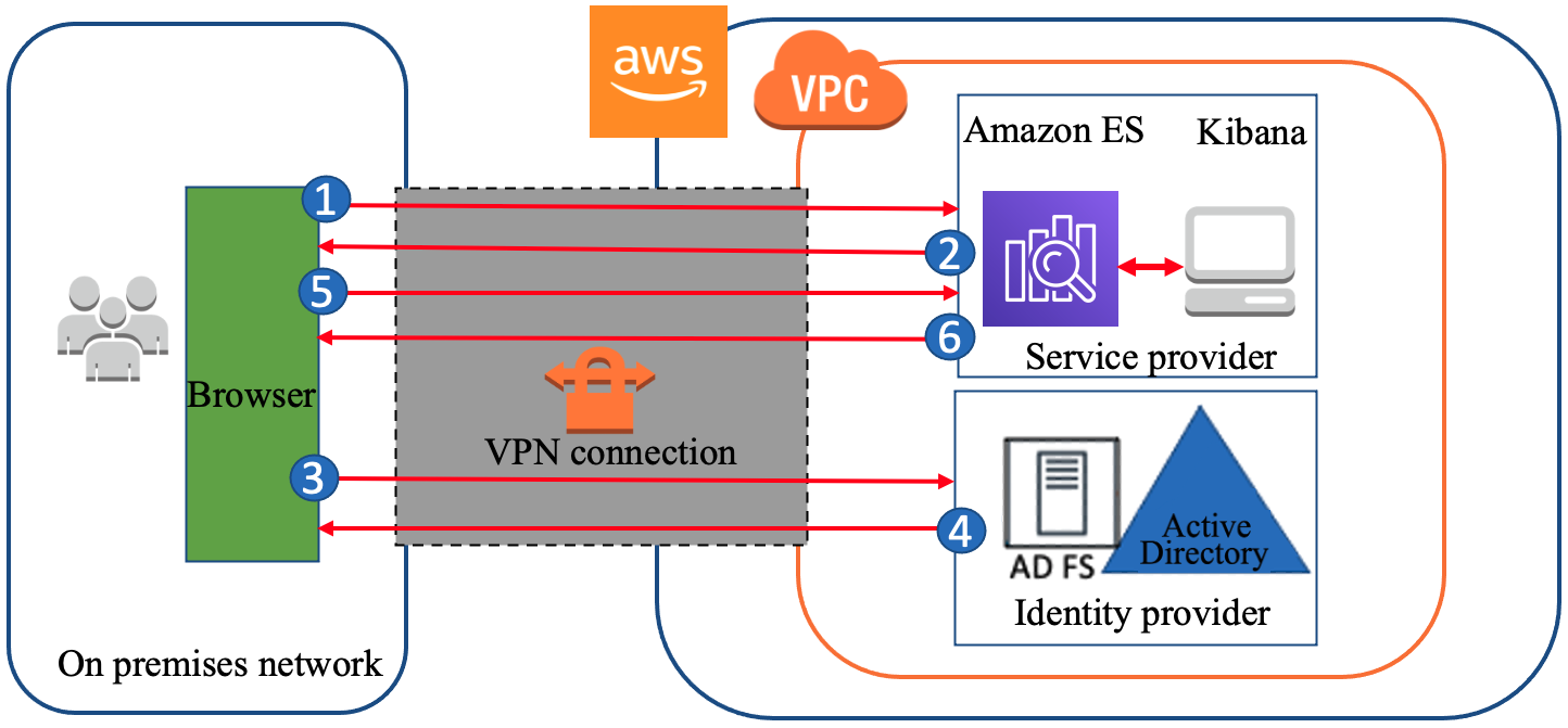
Solution architecture
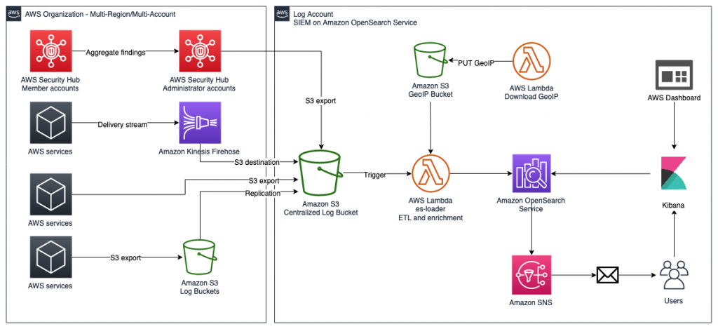
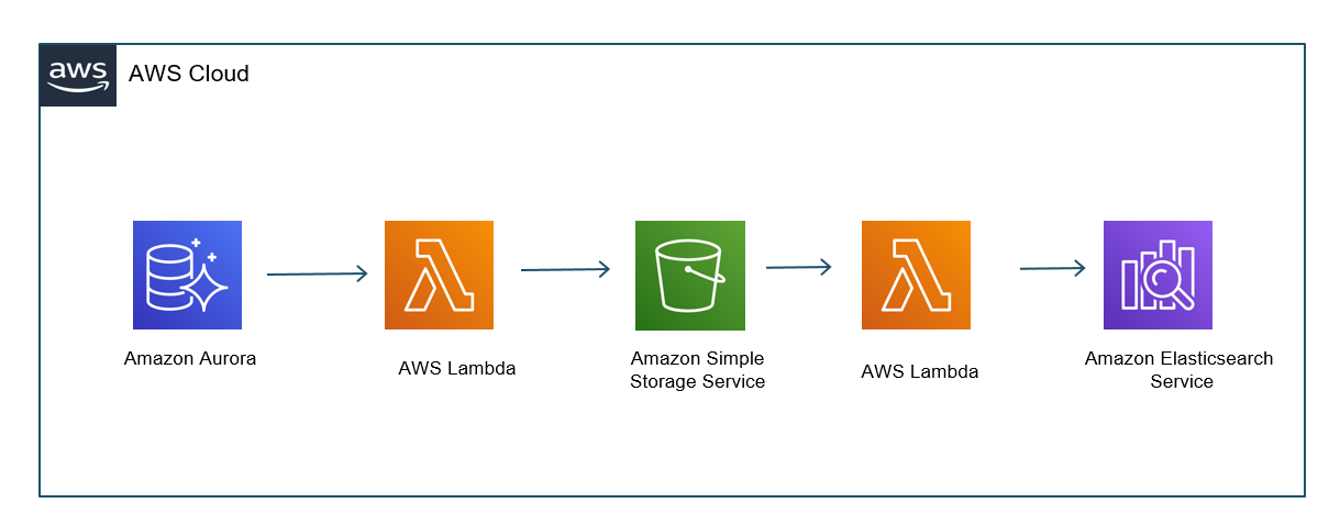
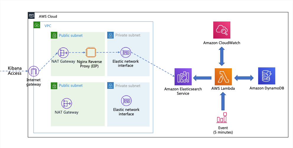
Figure 1: SIEM implementation on Amazon OpenSearch Service
The solution represented in Figure 1 shows the flexibility of integrations that are possible when you create a SIEM by using Amazon OpenSearch Service. The solution allows you to aggregate findings across multiple accounts, store findings in an S3 bucket indefinitely, and correlate multiple AWS and non-AWS services in one place for visualization. This post focuses on Security Hub’s integration with the solution, but the following AWS services are also able to integrate:
- AWS WAF
- Amazon CloudFront
- AWS CloudTrail
- Elastic Load Balancing (ELB)
- Amazon GuardDuty
- Amazon Relational Database Service (Amazon RDS)
- AWS Security Hub
- VPC Flow Logs
- Amazon WorkSpaces
Each of these services has its own dedicated dashboard within the OpenSearch SIEM solution. This makes it possible for customers to view findings and data that are relevant to each service that the SIEM tool is ingesting. OpenSearch Service also allows the customer to create aggregated dashboards, consolidating multiple services within a single dashboard, if needed.
Prerequisites
We recommend that you enable Security Hub and AWS Config across all of your accounts and Regions. For more information about how to do this, see the documentation for Security Hub and AWS Config. We also recommend that you use Security Hub and AWS Config integration with AWS Organizations to simplify the setup and automatically enable these services in all current and future accounts in your organization.
Launch the solution
In order to launch this solution within your environment, you can either launch the solution by using an AWS CloudFormation template, or by following the steps presented later in this post to customize the deployment to support integrations with non-AWS services, multi-Organization deployments, or launch within your existing OpenSearch Service environment.
To launch the solution, follow the instructions for SIEM on Amazon OpenSearch Service on GitHub.
Use the solution
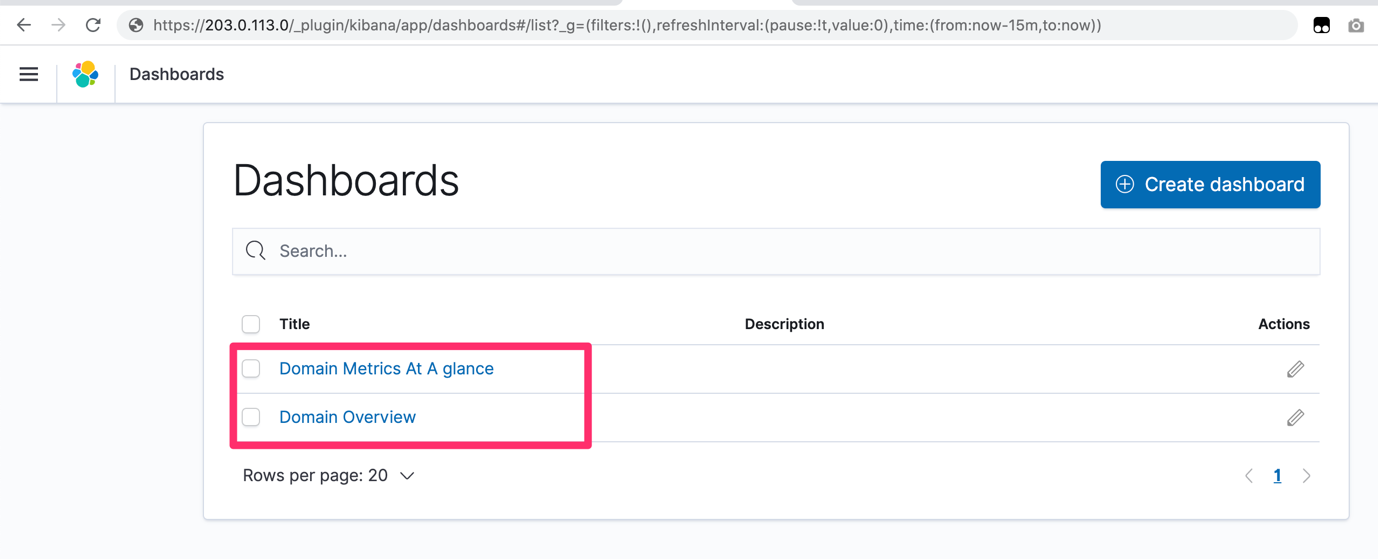
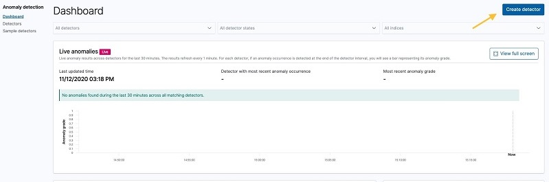
Before you start using the solution, we’ll show you how this solution appears in the Security Hub dashboard, as shown in Figure 2. Navigate here by following Step 3 from the GitHub README.
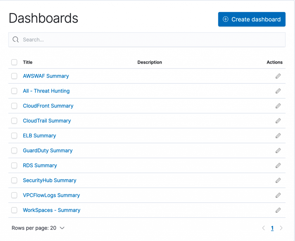
Figure 2: Pre-built dashboards within solution
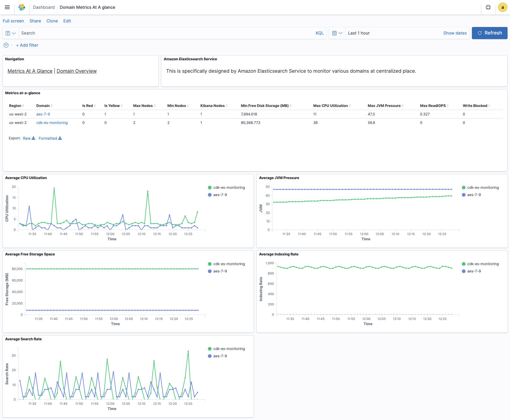
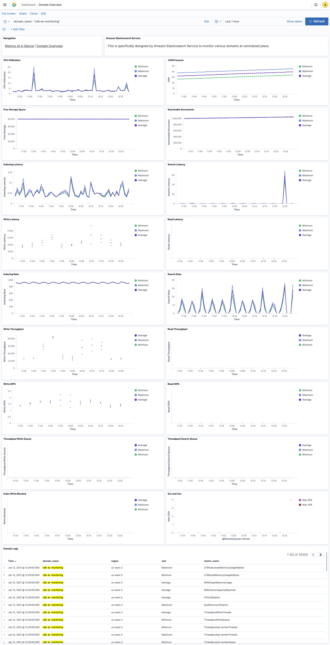
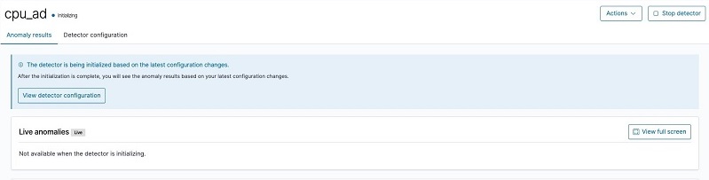
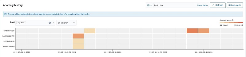
The Security Hub dashboard highlights all major components of the service within an OpenSearch Service dashboard environment. This includes supporting all of the service integrations that are available within Security Hub (such as GuardDuty, AWS Identity and Access Management (IAM) Access Analyzer, Amazon Inspector, Amazon Macie, and AWS Systems Manager Patch Manager). The dashboard displays both findings and security standards, and you can filter by AWS account, finding type, security standard, or service integration. Figure 3 shows an overview of the visual dashboard experience when you deploy the solution.
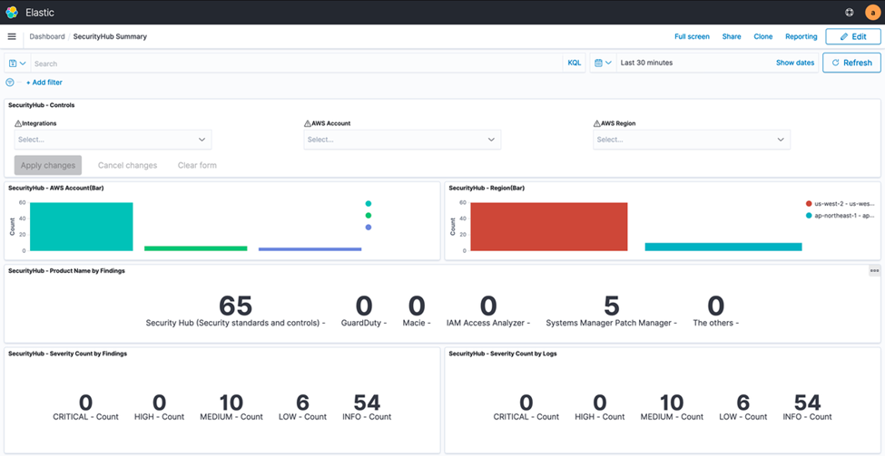
Figure 3: Dashboard preview
Use case 1: Correlate Security Hub findings with each other and other log sources and create alerts
This solution uses OpenSearch Service and Kibana to allow you to search through both Security Hub findings and logs from any other AWS and non-AWS systems. You can then create alerts within Kibana based on interesting correlations between Security Hub and any other logged events. Although Security Hub supports ingesting a vast number of integrations and findings, it cannot create correlation rules like a SIEM tool can. However, you can create such rules using SIEM on OpenSearch Service. It’s important to take a closer look when multiple AWS security services generate findings for a single resource, because this potentially indicates elevated risk or multiple risk vectors. Depending on your environment, the initial number of findings in Security Hub may be high, so you may need to prioritize which findings require immediate action. Security Hub natively gives you the ability to filter findings by resource, account, severity, and many other details.
As part of the findings, you can send notifications through alerts that are generated by SIEM on OpenSearch Service in several ways: Amazon Simple Notification Service (Amazon SNS) by consuming messages in an appropriate tool or configuring recipient email addresses, Amazon Chime, Slack (using AWS Chatbot) or custom webhook to your organization’s ticketing system. You can then respond to these new security incident-oriented findings through ticketing, chat, or incident management systems.
Solution overview for use case 1
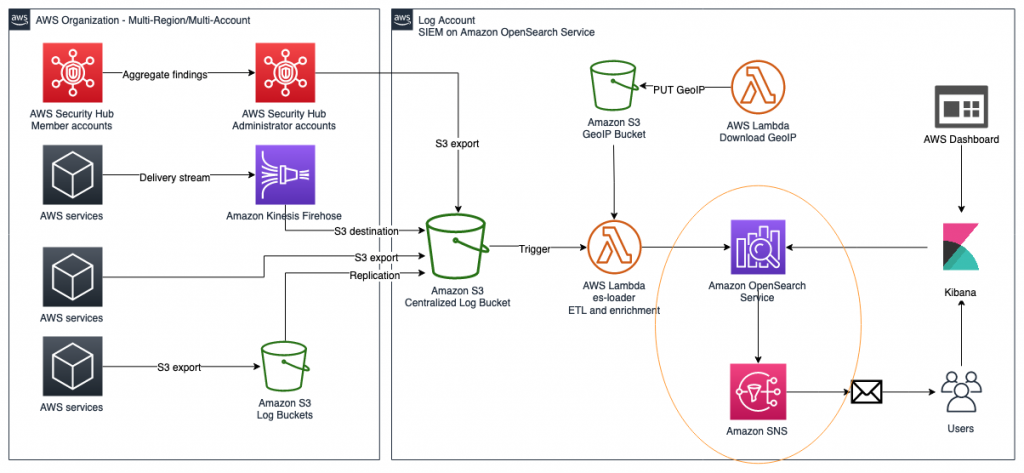
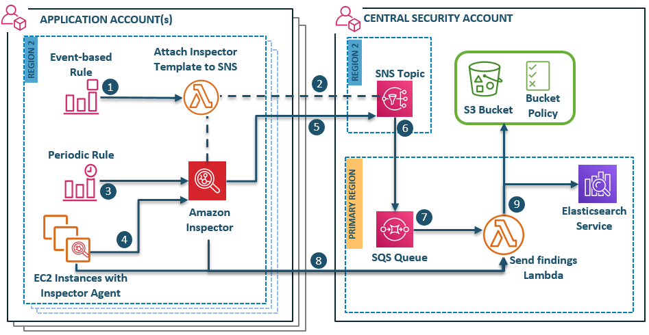
Figure 4: Solution overview diagram
Figure 4 gives an overview of the solution for use case 1. This solution requires that you have Security Hub and GuardDuty enabled in your AWS account. Logs from AWS services, including Security Hub, are ingested into an S3 bucket, then are automatically extracted, transformed, and loaded (ETL) and populated into the SIEM system that is running on OpenSearch Service using AWS Lambda. After capturing the logs, you will be able to visualize them on the dashboard and analyze correlations of multiple logs. Within the SIEM on OpenSearch Service solution, you will create a rule to detect failures, such as CloudTrail authentication failures in logs. Then, you will configure the solution to publish alerts to Amazon SNS and send emails when logs match rules.
Implement the solution for use case 1
You will now set up this workflow to alert you by email when logs in OpenSearch match certain rules that you create.
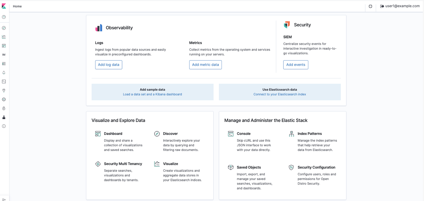
Step 1: Create and visualize findings in OpenSearch Dashboards
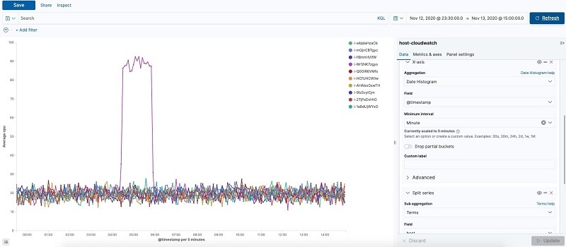
Security Hub and other AWS services export findings to Amazon S3 in a centralized log bucket. You can ingest logs from CloudTrail, VPC Flow Logs, and GuardDuty, which are often used in AWS security analytics. In this step, you import simulated security incident data in OpenSearch Dashboards, and use the dashboard to visualize the data in the logs.
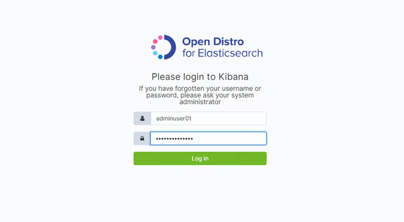
To navigate OpenSearch Dashboards
- Generate pseudo-security incidents. You can simulate the results by generating sample findings in GuardDuty.
- In OpenSearch Dashboards, go to the Discover screen. The Discover screen is divided into three major sections: Search bar, index/display field list, and time-series display, as shown in Figure 5.

Figure 5: OpenSearch Dashboards
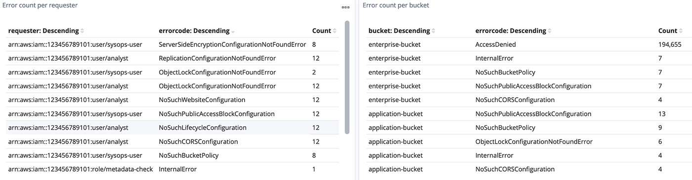
- In OpenSearch Dashboards, select log-aws-securityhub-* or log-aws-vpcflowlogs-* or log-aws-cloudtrail-* or any other index patterns and add event.module to the display field. event.module is a field that indicates where the log originates from. If you are collecting other threat information, such as Security Hub, @log-type is Security Hub, and event.module indicates where the log originated from (either Amazon Inspector or Amazon Macie for example). After you have added event.module, filter the desired Security Hub integrated service (for example, Amazon Inspector) to display. When testing the environment covered in this blog post outside a production context, you can use Kinesis Data Generator to generate sample user traffic. Other tools are also available.
- Select the following on the dashboard to see the visualized information:
- CloudTrail Summary
- VpcFlowLogs Summary
- GuardDuty Summary
- All – Threat Hunting

Step 2: Configure alerts to match log criteria
Next, you will configure alerts to match log criteria. First you need to set the destination for alerts, and then set what to monitor.
To configure alerts
- In OpenSearch Dashboards, in the left menu, choose Alerting.
- To add the details of SNS, on the Destinations tab, choose Add destinations, and enter the following parameters:
- Name: aes-siem-alert-destination
- Type: Amazon SNS
- SNS Alert: arn:aws:sns:<AWS-REGION>:<111111111111>:aes-siem-alert
- Replace <111111111111> with your AWS account ID and correct the Region name
- Replace <AWS-REGION> with the Region you are using, for example, eu-west-1
- IAM Role ARN: arn:aws:iam::<111111111111>:role/aes-siem-sns-role
- Replace &<111111111111> with your AWS account ID
- Choose Create to complete setting the alert destination.
Figure 6: Edit alert destination
- In OpenSearch Dashboards, in the left menu, select Alerting. You will now set what to monitor. Here you monitor a CloudTrail trail authentication failure. There are two normalized log times: @timestamp and event.ingested. The difference is between the log occurrence time (@timestamp) and the SIEM reception time (event.ingested). Use event.ingested for logs with a large time lag from occurrence to reception. You can specify flexible conditions by selecting Define using extraction query for the filter definition.
- On the Monitors tab, choose Create monitor.
- Enter the following parameters. If there is no description, use the default value.
- Name: Authentication failed
- Method of definition: Define using extraction query
- Indices: log-aws-cloudtrail-* (manual input, not pull-down)
- Define extraction query: Enter the following query.
- Enter the following remaining parameters of the monitor:
- Frequency: By interval
- Monitor schedule: Every 3 minutes
- Choose Create to create the monitor.

Step 3: Set up trigger to send email via Amazon SNS
Now you will set the alert firing condition, known as the trigger. This is the setting for alerting when the monitored conditions (Monitors) are met. By default, the alert will be triggered if the number of hits is greater than 0. In this step , you will not change it, only give it a name.
To set up the trigger
- Select Create trigger and for Trigger name, enter Authentication failed trigger.
- Scroll down to Configure actions.

Figure 7: Create trigger
- Set what the trigger should do (action). In this case, you want to publish to SNS. Set the following parameters for the body of the email
- Action name: Authentication failed action
- Destination: Choose aes-siem-alert-destination – (Amazon SNS)
- Message subject: (SIEM) Auth failure alert
- Action throttling: Select Enable action throttling, and set throttle action to only trigger every 10 minutes.
- Message: Copy and paste the following message into the text box. After pasting, choose Send test message at the bottom right of the screen to confirm that you can receive the test email.
Monitor ctx.monitor.name just entered alert status. Please investigate the issue.
Trigger: ctx.trigger.name
Severity: ctx.trigger.severity
@timestamp: ctx.results.0.hits.hits.0._source.@timestamp
event.action: ctx.results.0.hits.hits.0._source.event.action
error.message: ctx.results.0.hits.hits.0._source.error.message
count: ctx.results.0.hits.total.value
source.ip: ctx.results.0.hits.hits.0._source.source.ip
source.geo.country_name: ctx.results.0.hits.hits.0._source.source.geo.country_name
Figure 8: Configure actions
- You will receive an alert email in a few minutes. You can check the occurrence status, including the history, by the following method:
- In OpenSearch Dashboards, on the left menu, choose Alerting.
- On the Monitors tab, choose Authentication failed.
- You can check the status of the alert in the History pane.
Figure 9: Email alert


Use case 1 shows you how to correlate various Security Hub findings through this OpenSearch Service SIEM solution. However, you can take the solution a step further and build more complex correlation checks by following the procedure in the blog post Correlate security findings with AWS Security Hub and Amazon EventBridge. This information can then be ingested into this OpenSearch Service SIEM solution for viewing on a single screen.
Use case 2: Store findings for longer than 90 days after last update date
Security Hub has a maximum storage time of 90 days for events, but your organization might require data storage beyond that period, with flexibility to specify a custom retention period to meet your needs. The SIEM on Amazon OpenSearch Service solution creates a centralized S3 bucket where findings from Security Hub and various other services are collected and stored, and this bucket can be configured to store data as long as you require. The S3 bucket can persist data indefinitely, or you can create an S3 object lifecycle policy to set a custom retention timeframe. Lifecycle policies allow you to either transition objects between S3 storage classes or delete objects after a specified period. Alternatively, you can use S3 Intelligent-Tiering to allow the Amazon S3 service to move data between tiers, based on user access patterns.
Either lifecycle policies or S3 Intelligent-Tiering will allow you to optimize costs for data that is stored in S3, to keep data for archive or backup purposes when it is no longer available in Security Hub or OpenSearch Service. Within the solution, this centralized bucket is called aes-siem-xxxxxxxx-log and is configured to store data for OpenSearch Service to consume indefinitely. The Amazon S3 User Guide has instructions for configuring an S3 lifecycle policy that is explicitly defined by the user on the centralized bucket. Or you can follow the instructions for configuring intelligent tiering to allow the S3 service to manage which tier data is stored in automatically. After data is archived, you can use Amazon Athena to query the S3 bucket for historical information that has been removed from OpenSearch Service, because this S3 bucket acts as a centralized security event repository.
Use case 3: Aggregate findings across multiple administrator accounts
There are cases where you might have multiple Security Hub administrator accounts within one or multiple organizations. For these use cases, you can consolidate findings across these multiple Security Hub administrator accounts into a single S3 bucket for centralized storage, archive, backup, and querying. This gives you the ability to create a single SIEM on OpenSearch Service to minimize the number of monitoring tools you need. In order to do this, you can use S3 replication to automatically copy findings to a centralized S3 bucket. You can follow this detailed walkthrough on how to set up the correct bucket permissions in order to allow replication between the accounts. You can also follow this related blog post to configure cross-Region Security Hub findings that are centralized in a single S3 bucket, if cross-Region replication is appropriate for your security needs. With cross-account S3 replication set up for Security Hub archived event data, you can import data from the centralized S3 bucket into OpenSearch Service by using the Lambda function within the solution in this blog post. This Lambda function automatically normalizes and enriches the log data and imports it into OpenSearch Service, so that users only need to configure data storage in the S3 bucket, and the Lambda function will automatically import the data.
Conclusion
In this blog post, we showed how you can use Security Hub with a SIEM to store findings for longer than 90 days, aggregate findings across multiple administrator accounts, and correlate Security Hub findings with each other and other log sources. We used the solution to walk through building the SIEM and explained how Security Hub could be used within that solution to add greater flexibility. This post describes one solution to create your own SIEM using OpenSearch Service; however, we also recommend that you read the blog post Visualize AWS Security Hub Findings using Analytics and Business Intelligence Tools, in order to see a different method of consolidating and visualizing insights from Security Hub.
To learn more, you can also try out this solution through the new SIEM on AWS OpenSearch Service workshop.
If you have feedback about this blog post, submit comments in the Comments section below. If you have questions about this blog post, please start a new thread on the Security Hub forum or contact AWS Support.
If you have feedback about this post, submit comments in the Comments section below. If you have questions about this post, contact AWS Support.
Want more AWS Security news? Follow us on Twitter.


 Zachariah Elliott works as a Solutions Architect focusing on EdTech at AWS. He is passionate about helping customers build Well-Architected solutions on AWS. He is also part of the IoT Subject Matter Expert community at AWS and loves helping customers develop unique IoT-based solutions.
 Pranusha Manchala is a Solutions Architect at AWS who works with education companies. She has worked with many EdTech customers and provided them with architectural guidance for building highly scalable and cost-optimized applications on AWS. She found her interests in machine learning and started to dive deep into this technology. She enjoys cooking, baking, and outdoor activities in her free time.

 Kapil Pendse is a Senior Solutions Architect with Amazon Web Services (Singapore) and has over 15 years of experience building technology solutions across multiple domains such as cloud computing, embedded systems, and machine learning. In his free time, Kapil likes to bike along Singapore’s coastal parks and enjoys the occasional company of otters.


 Jon Handler (@_searchgeek) is a Principal Solutions Architect at Amazon Web Services based in Palo Alto, CA. Jon works closely with the CloudSearch and Elasticsearch teams, providing help and guidance to a broad range of customers who have search workloads that they want to move to the AWS Cloud. Prior to joining AWS, Jon’s career as a software developer included four years of coding a large-scale, eCommerce search engine.
 Prashant Agrawal is a Specialist Solutions Architect at Amazon Web Services based in Seattle, WA.. Prashant works closely with Amazon Elasticsearch team, helping customers migrate their workloads to the AWS Cloud. Before joining AWS, Prashant helped various customers use Elasticsearch for their search and analytics use cases.


 Conclusion
 Jeff Wright is a Software Development Engineer at Amazon Web Services where he works on the Search Services team. His interests are designing and building robust, scalable distributed applications. Jeff is a contributor to Open Distro for Elasticsearch.
 Kowshik Nagarajaan is a Software Development Engineer at Amazon Web Services where he works on the Search Services team. His interests are building and automating distributed analytics applications. Kowshik is a contributor to Open Distro for Elasticsearch.
 Anush Krishnamurthy is an Engineering Manager working on the Search Services team at Amazon Web Services.


 Viraj Phanse is a product management leader at Amazon Web Services for Search Services/Analytics. An avid foodie, he loves trying cuisines from around the globe. In his free time, he loves to play his keyboard and travel.

 Chris Swierczewski is an applied scientist at AWS. He enjoys reading, weightlifting, painting, and board games.


 Satya Vajrapu is a DevOps Consultant with Amazon Web Services. He works with AWS customers to help design and develop various practices and tools in the DevOps toolchain.

 Vijay Injam is a Data Architect with Amazon Web Services.
  Kevin Fallis is an AWS specialist search solutions architect. His passion at AWS is to help customers leverage the correct mix of AWS services to achieve success for their business goals. His after-work activities include family, DIY projects, carpentry, playing drums, and all things music.


 Mahesh Goyal is a Data Architect in Big Data at AWS. He works with customers in their journey to the cloud with a focus on big data and data warehouses. In his spare time, Mahesh likes to listen to music and explore new food places with his family.