All posts by Ajay Vohra

Automate secure access to Amazon MWAA environments using existing OpenID Connect single-sign-on authentication and authorization

Post Syndicated from Ajay Vohra original https://aws.amazon.com/blogs/big-data/automate-secure-access-to-amazon-mwaa-environments-using-existing-openid-connect-single-sign-on-authentication-and-authorization/

Customers use Amazon Managed Workflows for Apache Airflow (Amazon MWAA) to run Apache Airflow at scale in the cloud. They want to use their existing login solutions developed using OpenID Connect (OIDC) providers with Amazon MWAA; this allows them to provide a uniform authentication and single sign-on (SSO) experience using their adopted identity providers (IdP) across AWS services. For ease of use for end-users of Amazon MWAA, organizations configure a custom domain endpoint to their Apache Airflow UI endpoint. For teams operating and managing multiple Amazon MWAA environments, securing and customizing each environment is a repetitive but necessary task. Automation through infrastructure as code (IaC) can alleviate this heavy lifting to achieve consistency at scale.

This post describes how you can integrate your organization’s existing OIDC-based IdPs with Amazon MWAA to grant secure access to your existing Amazon MWAA environments. Furthermore, you can use the solution to provision new Amazon MWAA environments with the built-in OIDC-based IdP integrations. This approach allows you to securely provide access to your new or existing Amazon MWAA environments without requiring AWS credentials for end-users.

Overview of Amazon MWAA environments

Managing multiple user names and passwords can be difficult—this is where SSO authentication and authorization comes in. OIDC is a widely used standard for SSO, and it’s possible to use OIDC SSO authentication and authorization to access Apache Airflow UI across multiple Amazon MWAA environments.

When you provision an Amazon MWAA environment, you can choose public or private Apache Airflow UI access mode. Private access mode is typically used by customers that require restricting access from only within their virtual private cloud (VPC). When you use public access mode, the access to the Apache Airflow UI is available from the internet, in the same way as an AWS Management Console page. Internet access is needed when access is required outside of a corporate network.

Regardless of the access mode, authorization to the Apache Airflow UI in Amazon MWAA is integrated with AWS Identity and Access Management (IAM). All requests made to the Apache Airflow UI need to have valid AWS session credentials with an assumed IAM role that has permissions to access the corresponding Apache Airflow environment. For more details on the permissions policies needed to access the Apache Airflow UI, refer to Apache Airflow UI access policy: AmazonMWAAWebServerAccess.

Different user personas such as developers, data scientists, system operators, or architects in your organization may need access to the Apache Airflow UI. In some organizations, not all employees have access to the AWS console. It’s fairly common that employees who don’t have AWS credentials may also need access to the Apache Airflow UI that Amazon MWAA exposes.

In addition, many organizations have multiple Amazon MWAA environments. It’s common to have an Amazon MWAA environment setup per application or team. Each of these Amazon MWAA environments can be run in different deployment environments like development, staging, and production. For large organizations, you can easily envision a scenario where there is a need to manage multiple Amazon MWAA environments. Organizations need to provide secure access to all of their Amazon MWAA environments using their existing OIDC provider.

Solution Overview

The solution architecture integrates an existing OIDC provider to provide authentication for accessing the Amazon MWAA Apache Airflow UI. This allows users to log in to the Apache Airflow UI using their OIDC credentials. From a system perspective, this means that Amazon MWAA can integrate with an existing OIDC provider rather than having to create and manage an isolated user authentication and authorization through IAM internally.

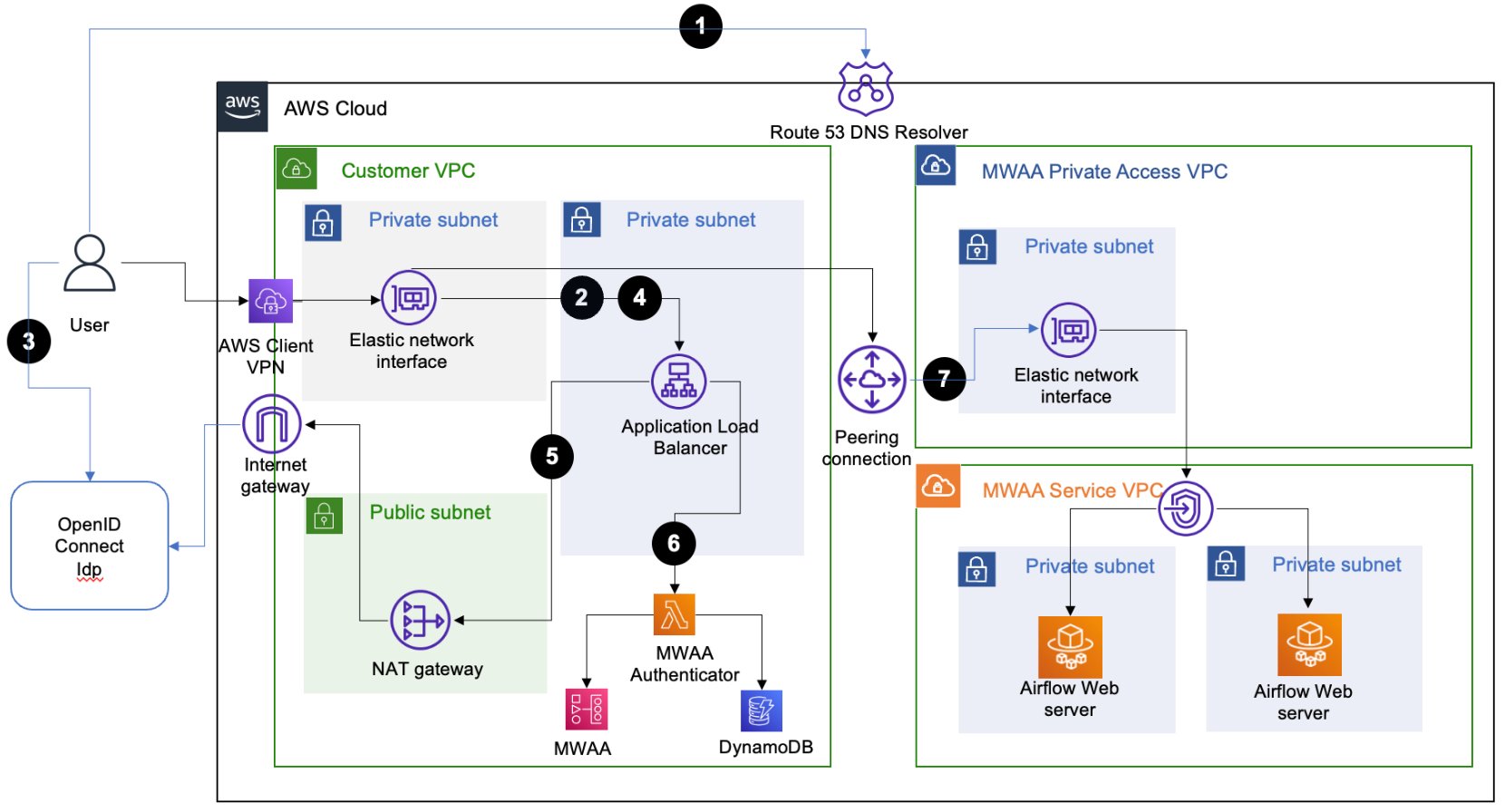
The solution architecture relies on an Application Load Balancer (ALB) setup with a fully qualified domain name (FQDN) with public (internet) or private access. This ALB provides SSO access to multiple Amazon MWAA environments. The user-agent (web browser) call flow for accessing an Apache Airflow UI console to the target Amazon MWAA environment includes the following steps:

  1. The user-agent resolves the ALB domain name from the Domain Name System (DNS) resolver.
  2. The user-agent sends a login request to the ALB path /aws_mwaa/aws-console-sso with a set of query parameters populated. The request uses the required parameters mwaa_env and rbac_role as placeholders for the target Amazon MWAA environment and the Apache Airflow role-based access control (RBAC) role, respectively.
  3. Once it receives the request, the ALB redirects the user-agent to the OIDC IdP authentication endpoint. The user-agent authenticates with the OIDC IdP with the existing user name and password.
  4. If user authentication is successful, the OIDC IdP redirects the user-agent back to the configured ALB with a redirect_url with the authorization code included in the URL.
  5. The ALB uses the authorization code received to obtain the access_token and OpenID JWT token with openid email scope from the OIDC IdP. It then forwards the login request to the Amazon MWAA authenticator AWS Lambda function with the JWT token included in the request header in the x-amzn-oidc-data parameter.
  6. The Lambda function verifies the JWT token found in the request header using ALB public keys. The function subsequently authorizes the authenticated user for the requested mwaa_env and rbac_role stored in an Amazon DynamoDB table. The use of DynamoDB for authorization here is optional; the Lambda code function is_allowed can be customized to use other authorization mechanisms.
  7. The Amazon MWAA authenticator Lambda function redirects the user-agent to the Apache Airflow UI console in the requested Amazon MWAA environment with the login token in the redirect URL. Additionally, the function provides the logout functionality.

Amazon MWAA public network access mode

For the Amazon MWAA environments configured with public access mode, the user agent uses public routing over the internet to connect to the ALB hosted in a public subnet.

The following diagram illustrates the solution architecture with a numbered call flow sequence for internet network reachability.

Amazon MWAA public network access mode architecture diagram

Amazon MWAA private network access mode

For Amazon MWAA environments configured with private access mode, the user agent uses private routing over a dedicated AWS Direct Connect or AWS Client VPN to connect to the ALB hosted in a private subnet.

The following diagram shows the solution architecture for Client VPN network reachability.

Amazon MWAA private network access mode architecture diagram

Automation through infrastructure as code

To make setting up this solution easier, we have released a pre-built solution that automates the tasks involved. The solution has been built using the AWS Cloud Development Kit (AWS CDK) using the Python programming language. The solution is available in our GitHub repository and helps you achieve the following:

  • Set up a secure ALB to provide OIDC-based SSO to your existing Amazon MWAA environment with default Apache Airflow Admin role-based access.
  • Create new Amazon MWAA environments along with an ALB and an authenticator Lambda function that provides OIDC-based SSO support. With the customization provided, you can define the number of Amazon MWAA environments to create. Additionally, you can customize the type of Amazon MWAA environments created, including defining the hosting VPC configuration, environment name, Apache Airflow UI access mode, environment class, auto scaling, and logging configurations.

The solution offers a number of customization options, which can be specified in the cdk.context.json file. Follow the setup instructions to complete the integration to your existing Amazon MWAA environments or create new Amazon MWAA environments with SSO enabled. The setup process creates an ALB with an HTTPS listener that provides the user access endpoint. You have the option to define the type of ALB that you need. You can define whether your ALB will be public facing (internet accessible) or private facing (only accessible within the VPC). It is recommended to use a private ALB with your new or existing Amazon MWAA environments configured using private UI access mode.

The following sections describe the specific implementation steps and customization options for each use case.

Prerequisites

Before you continue with the installation steps, make sure you have completed all prerequisites and run the setup-venv script as outlined within the README.md file of the GitHub repository.

Integrate to a single existing Amazon MWAA environment

If you’re integrating with a single existing Amazon MWAA environment, follow the guides in the Quick start section. You must specify the same ALB VPC as that of your existing Amazon MWAA VPC. You can specify the default Apache Airflow RBAC role that all users will assume. The ALB with an HTTPS listener is configured within your existing Amazon MWAA VPC.

Integrate to multiple existing Amazon MWAA environments

To connect to multiple existing Amazon MWAA environments, specify only the Amazon MWAA environment name in the JSON file. The setup process will create a new VPC with subnets hosting the ALB and the listener. You must define the CIDR range for this ALB VPC such that it doesn’t overlap with the VPC CIDR range of your existing Amazon MWAA VPCs.

When the setup steps are complete, implement the post-deployment configuration steps. This includes adding the ALB CNAME record to the Amazon Route 53 DNS domain.

For integrating with Amazon MWAA environments configured using private access mode, there are additional steps that need to be configured. These include configuring VPC peering and subnet routes between the new ALB VPC and the existing Amazon MWAA VPC. Additionally, you need to configure network connectivity from your user-agent to the private ALB endpoint resolved by your DNS domain.

Create new Amazon MWAA environments

You can configure the new Amazon MWAA environments you want to provision through this solution. The cdk.context.json file defines a dictionary entry in the MwaaEnvironments array. Configure the details that you need for each of the Amazon MWAA environments. The setup process creates an ALB VPC, ALB with an HTTPS listener, Lambda authorizer function, DynamoDB table, and respective Amazon MWAA VPCs and Amazon MWAA environments in them. Furthermore, it creates the VPC peering connection between the ALB VPC and the Amazon MWAA VPC.

If you want to create Amazon MWAA environments with private access mode, the ALB VPC CIDR range specified must not overlap with the Amazon MWAA VPC CIDR range. This is required for the automatic peering connection to succeed. It can take between 20–30 minutes for each Amazon MWAA environment to finish creating.

When the environment creation processes are complete, run the post-deployment configuration steps. One of the steps here is to add authorization records to the created DynamoDB table for your users. You need to define the Apache Airflow rbac_role for each of your end-users, which the Lambda authorizer function matches to provide the requisite access.

Verify access

Once you’ve completed with the post-deployment steps, you can log in to the URL using your ALB FQDN. For example, If your ALB FQDN is alb-sso-mwaa.example.com, you can log in to your target Amazon MWAA environment, named Env1, assuming a specific Apache Airflow RBAC role (such as Admin), using the following URL: https://alb-sso-mwaa.example.com/aws_mwaa/aws-console-sso?mwaa_env=Env1&rbac_role=Admin. For the Amazon MWAA environments that this solution created, you need to have appropriate Apache Airflow rbac_role entries in your DynamoDB table.

The solution also provides a logout feature. To log out from an Apache Airflow console, use the normal Apache Airflow console logout. To log out from the ALB, you can, for example, use the URL https://alb-sso-mwaa.example.com/logout.

Clean up

Follow the readme documented steps in the section Destroy CDK stacks in the GitHub repo, which shows how to clean up the artifacts created via the AWS CDK deployments. Remember to revert any manual configurations, like VPC peering connections, that you might have made after the deployments.

Conclusion

This post provided a solution to integrate your organization’s OIDC-based IdPs with Amazon MWAA to grant secure access to multiple Amazon MWAA environments. We walked through the solution that solves this problem using infrastructure as code. This solution allows different end-user personas in your organization to access the Amazon MWAA Apache Airflow UI using OIDC SSO.

To use the solution for your own environments, refer to Application load balancer single-sign-on for Amazon MWAA. For additional code examples on Amazon MWAA, refer to Amazon MWAA code examples.


About the Authors

Ajay Vohra is a Principal Prototyping Architect specializing in perception machine learning for autonomous vehicle development. Prior to Amazon, Ajay worked in the area of massively parallel grid-computing for financial risk modeling.

Jaswanth Kumar is a customer-obsessed Cloud Application Architect at AWS in NY. Jaswanth excels in application refactoring and migration, with expertise in containers and serverless solutions, coupled with a Masters Degree in Applied Computer Science.

Aneel Murari is a Sr. Serverless Specialist Solution Architect at AWS based in the Washington, D.C. area. He has over 18 years of software development and architecture experience and holds a graduate degree in Computer Science. Aneel helps AWS customers orchestrate their workflows on Amazon Managed Apache Airflow (MWAA) in a secure, cost effective and performance optimized manner.

Parnab Basak is a Solutions Architect and a Serverless Specialist at AWS. He specializes in creating new solutions that are cloud native using modern software development practices like serverless, DevOps, and analytics. Parnab works closely in the analytics and integration services space helping customers adopt AWS services for their workflow orchestration needs.

Field Notes: Building a Data Service for Autonomous Driving Systems Development using Amazon EKS

Post Syndicated from Ajay Vohra original https://aws.amazon.com/blogs/architecture/field-notes-building-a-data-service-for-autonomous-driving-systems-development-using-amazon-eks/

Many aspects of autonomous driving (AD) system development are based on data that capture real-life driving scenarios. Therefore, research and development professionals working on AD systems need to handle an ever-changing array of interesting datasets composed from the real-life driving data.  In this blog post, we address a key problem in AD system development, which is how to dynamically compose interesting datasets from real-life driving data and serve them at scale in near real-time.

The first challenge in composing large interesting datasets is high latency. If you have to wait for the entire dataset to be composed before you can start consuming the dataset, you may have to wait for several minutes, or even hours. This latency slows down AD system research and development. The second challenge is creating a data service that can cost-efficiently serve the dynamically composed datasets at scale. In this blog post, we propose solutions to both these challenges.

For the challenge of high latency, we propose dynamically composing the data sets as chunked data streams, and serving them using a Amazon FSx for Lustre high-performance file-system. Chunked data streams immediately solve the latency issue, because you do not need to compose the entire stream before it can be consumed. For the challenge of cost-efficiently serving the datasets at scale, we propose using Amazon EKS with auto-scaling features.

Overview of the Data Service Architecture

The data service described in this post dynamically composes and serves data streams of selected sensor modalities for a specified drive scene selected from the A2D2 driving dataset. The data stream is dynamically composed from the extracted A2D2 drive scene data stored in Amazon S3 object data store, and the accompanying meta-data stored in an Amazon Redshift data warehouse. While the data service described in this post uses the Robot Operating System (ROS), the data service can be easily adapted for use with other robotic systems.

The data service runs in Kubernetes Pods in an Amazon EKS cluster configured to use a Horizontal Pod Autoscaler and EKS Cluster Autoscaler. An Amazon Managed Service For Apache Kafka (MSK) cluster provides the communication channel between the data service, and the data clients. The data service implements a request-response paradigm over Apache Kafka topics. However, the response data is not sent back over the Kafka topics. Instead, the data service stages the response data in Amazon S3, Amazon FSx for Lustre, or Amazon EFS, as specified in the data client request, and only the location of the staged response data is sent back to the data client over the Kafka topics. The data client directly reads the response data from its staged location.

The data client running in a ROS enabled Amazon EC2 instance plays back the received data stream into ROS topics, whereby it can be nominally consumed by any ROS node subscribing to the ROS topics. The solution architecture diagram for the data service is shown in Figure 1.

Figure 1. Data service solution architecture with default configuration

Figure 1 – Data service solution architecture with default configuration

Data Client Request

Imagine the data client wants to request drive scene data in ROS bag file format from A2D2 autonomous driving dataset for vehicle id a2d2, drive scene id 20190401145936, starting at timestamp 1554121593909500 (microseconds) , and stopping at timestamp 1554122334971448 (microseconds). The data client wants the response to include data only from the camera/front_left sensor encoded in sensor_msgs/Image ROS data type, and the lidar/front_left  sensor encoded in sensor_msgs/PointCloud2 ROS data type. The data client wants the response data to be streamed back chunked in series of rosbag files, each file spanning 1000000 microseconds of the drive scene. The data client wants the chunked response rosbag files to be staged on a shared Amazon FSx for Lustre file system.

Finally, the data client wants the camera/front_left sensor data to be played back on /a2d2/camera/front_left ROS topic, and the lidar/front_left  sensor data to be played back on /a2d2/lidar/front_left ROS topic.

The data client can encode such a data request using the following JSON object, and send it to the Kafka bootstrap servers  b-1.msk-cluster-1:9092,b-2.msk-cluster-1:9092 on the Apache Kafka topic named a2d2.

{
 "servers": "b-1.msk-cluster-1:9092,b-2.msk-cluster-1:9092",
 "requests": [{
    "kafka_topic": "a2d2", 
    "vehicle_id": "a2d2",
    "scene_id": "20190401145936",
    "sensor_id": ["lidar/front_left", "camera/front_left"],
    "start_ts": 1554121593909500, 
    "stop_ts": 1554122334971448,
    "ros_topic": {"lidar/front_left": "/a2d2/lidar/front_left", 
    "camera/front_left": "/a2d2/camera/front_left"},
    "data_type": {"lidar/front_left": "sensor_msgs/PointCloud2",
    "camera/front_left": "sensor_msgs/Image"},
    "step": 1000000,
    "accept": "fsx/multipart/rosbag",
    "preview": false
 }]
}

At any given time, one or more EKS pods in the data service are listening for messages on the Kafka topic a2d2. The EKS pod that picks the request message responds to the request by composing the requested data as a series of rosbag files, and staging them on FSx for Lustre, as requested in the  "accept": "fsx/multipart/rosbag" field.

Each rosbag in the response is dynamically composed from the drive scene data stored in Amazon S3, using the meta-data stored in Amazon Redshift. Each rosbag contains drive scene data for a single time step. In the preceding example, the time step is specified as "step": 1000000 (microseconds).

Visualizing the Data Service Response

If a human is interested in visualizing the data response, one can use any ROS visualization tool. One such tool is rviz. This tool can be run on the ROS desktop. In the following screenshot, we show the visualization of the response using rviz tool for the example data request shown previously.

Figure 2. Visualization of response using rviz tool

Figure 2 – Visualization of response using rviz tool

Dynamically Transforming the Coordinate Frames

The data service supports dynamically transforming the composed data from one coordinate frame to another frame. A typical use case is to transform the data from a sensor specific coordinate frame to AV (ego) coordinate frame. Such transformation request can be included in the data client request.

For example, imagine the data client wants to compose a data stream from all the LiDAR sensors, and transform the point cloud  data into the vehicle’s coordinate frame. The example configuration c-config-lidar.json allows you to do that. Following is a visualization of the LiDAR point cloud data transformed to the vehicle coordinate frame and visualized in the rviz tool  from a top-down perspective.

Figure 3. Top-down rviz visualization of point-cloud data transformed to ego vehicle view

Figure 3 –  Top-down rviz visualization of point-cloud data transformed to ego vehicle view

Walkthrough

In this walkthrough, we use the A2D2 autonomous driving dataset. The complete code for this walk-through and reference documentation is available in the associated Github repository. So before we get into the walk-through, clone the  Github repository on your laptop using the Git clone command. Next, ensure these prerequisites are satisfied.

The approximate cost of the walk-through of this tutorial with default configuration is US $2,000. The actual cost may vary considerably based on actual configuration, and the duration used for the walk-through.

Configure the data service

To configure the data service, we need to create a new AWS CloudFormation stack in the AWS console using the cfn/mozart.yml template from the cloned repository on your laptop.

This template creates AWS Identity and Access Management (IAM) resources, so when you create the CloudFormation Stack using the console, in the review step, you must check I acknowledge that AWS CloudFormation might create IAM resources. The stack input parameters you must specify are the following:

Parameter Name table

For all other stack input parameters, default values are recommended during the first walkthrough. Review the complete list of all the template input parameters in the Github repository reference.

  • Once the stack status in CloudFormation console is CREATE_COMPLETE, find the ROS desktop instance launched in your stack in the Amazon EC2 console, and connect to the instance using SSH as user ubuntu, using your SSH key pair. The ROS desktop instance is named as <name-of-stack>-desktop.
  • When you connect to the ROS desktop using SSH, and you see the message "Cloud init in progress. Machine will REBOOT after cloud init is complete!!", disconnect and try later after about 20 minutes. The desktop installs the NICE DCV server on first-time startup, and reboots after the install is complete.
  • If the message NICE DCV server is enabled!appears, run the command sudo passwd ubuntu to set a new strong password for user ubuntu. Now you are ready to connect to the desktop using the NICE DCV client.
  • Download and install the NICE DCV client on your laptop.
  • Use the NICE DCV Client to login to the desktop as user ubuntu
  • When you first login to the desktop using the NICE DCV client, you may be asked if you would like to upgrade the OS version. Do not upgrade the OS version.

Now you are ready to proceed with the following steps. For all the commands in this blog, we assume the working directory to be ~/amazon-eks-autonomous-driving-data-service on the ROS desktop.

If you used an IAM role to create the stack above, you must manually configure the credentials associated with the IAM role in the ~/.aws/credentials file with the following fields:

aws_access_key_id=

aws_secret_access_key=

aws_session_token=

If you used an IAM user to create the stack, you do not have to manually configure the credentials. In the working directory, run the command:

    ./scripts/configure-eks-auth.sh

When successfully running this command, the following confirmation appears AWS Credentials Removed.

Configure the EKS cluster environment

In this step, we configure the EKS cluster environment by running the command:

    ./scripts/setup-dev.sh

This step also builds and pushes the data service container image into Amazon ECR.

Prepare the A2D2 data

Before we can run the A2D2 data service, we need to extract the raw A2D2 data into your S3 bucket, extract the metadata from the raw data, and upload the metadata into the Redshift cluster. We execute these three steps using an AWS Step Functions state machine. To create and run the AWS Step Functions state machine, run the following command in the working directory:

    ./scripts/a2d2-etl-steps.sh

Note the executionArn of the state machine execution in the output of the previous command. To check the status of the execution, use following command, replacing executionArn below with your value:

The state machine execution time depends on many variable factors, and may take anywhere from 4 – 24 hours, or possibly longer. All the AWS Batch jobs started as part of the state machine automatically reattempt in case of failure.

Run the data service

The data service is deployed using a Helm Chart, and runs as a kubernetes deployment in EKS. To start the data service, execute the following command in the working directory:

    kubectl get pods -n a2d2

Run the data service client

To visualize the response data requested by the A2D2 data client, we will use the rviz tool on the ROS desktop. Open a terminal on the desktop, and run rviz.

In the rviz tool, use File>Open Config to select /home/ubuntu/amazon-eks-autonomous-driving-data-service/a2d2/config/a2d2.rviz as the rviz config. You should notice that the rviz tool is now configured with two areas, one for visualizing image data, and the other for visualizing point cloud data.

To run the data client, open a new terminal on the desktop, and execute the following command in the root directory of the cloned Github repository on the ROS desktop:

python ./a2d2/src/data_client.py --config ./a2d2/config/c-config-ex1.json 1>/tmp/a.out 2>&1 & 

After a brief delay, you should be able to preview the response data in the rviz tool. You can set "preview": false in the data client config file, ./a2d2/config/c-config-ex1.json, and rerun the preceding command to view the complete response. For maximum performance, pre-load S3 data to FSx for Lustre.

Hard reset of the data service

This step is for reference purposes. If at any time you need to do a hard reset of the data service, you can do so by executing:

    helm delete a2d2-data-service

This will delete all data service EKS pods immediately. All in-flight service responses will be aborted. Because the connection between the data client and data service is asynchronous, the data clients may wait indefinitely, and you may need to cleanup the data client processes manually on the ROS desktop using operating system tools. Note, each data client instance spawns multiple Python processes. You may also want to cleanup /fsx/rosbag directory.

Clean Up

When you no longer need the data service,  delete the AWS CloudFormation stack from the AWS CloudFormation console. Deleting the stack will shut down the desktop instance, and delete the EFS and FSx for Lustre file-systems created in the stack. The Amazon S3 bucket is not deleted.

Conclusion

In this post, we demonstrated how to build a data service that can dynamically compose near real-time chunked data streams at scale using EKS, Redshift, MSK, and FSx for Lustre. By using a data service, you increase agility, flexibility and cost-efficiency in AD system research and development.

Related reading: Field Notes: Deploy and Visualize ROS Bag Data on AWS using rviz and Webviz for Autonomous Driving

Field Notes provides hands-on technical guidance from AWS Solutions Architects, consultants, and technical account managers, based on their experiences in the field solving real-world business problems for customers.

Field Notes: Launch a Fully Configured AWS Deep Learning Desktop with NICE DCV

Post Syndicated from Ajay Vohra original https://aws.amazon.com/blogs/architecture/field-notes-launch-a-fully-configured-aws-deep-learning-desktop-with-nice-dcv/

You want to start quickly when doing deep learning using GPU-activated Elastic Compute Cloud (Amazon EC2) instances in the AWS Cloud. Although AWS provides end-to-end machine learning (ML) in Amazon SageMaker, working at the deep learning frameworks level, the quickest way to start is with AWS Deep Learning AMIs (DLAMIs), which provide preconfigured Conda environments for most of the popular frameworks.

DLAMIs make it straightforward to launch Amazon EC2 instances, but these instances do not automatically provide the high-performance graphics visualization required during deep learning research. Additionally, they are not preconfigured to use AWS storage services or SageMaker. This post explains how you can launch a fully-configured deep learning desktop in the AWS Cloud. Not only is this desktop preconfigured with the popular frameworks such as TensorFlow, PyTorch, and Apache MXNet, but it is also enabled for high-performance graphics visualization. NICE DCV is the remote display protocol used for visualization. In addition, it is preconfigured to use AWS storage services and SageMaker.

Overview of the Solution

The deep learning desktop described in this solution is ready for research and development of deep neural networks (DNNs) and their visualization. You no longer need to set up low-level drivers, libraries, and frameworks, or configure secure access to AWS storage services and SageMaker. The desktop has preconfigured access to your data in a Simple Storage Service (Amazon S3) bucket, and a shared Amazon Elastic File System (Amazon EFS) is automatically attached to the desktop. It is automatically configured to access SageMaker for ML services, and provides you with the ability to prepare the data needed for deep learning, and to research, develop, build, and debug your DNNs. You can use all the advanced capabilities of SageMaker from your deep learning desktop. The following diagram shows the reference architecture for this solution.

Reference Architecture to Launch a Fully Configured AWS Deep Learning Desktop with NICE DCV

Figure 1 – Architecture overview of the solution to launch a fully configured AWS Deep Learning Desktop with NICE DCV

The deep learning desktop solution discussed in this post is contained in a single AWS CloudFormation template. To launch the solution, you create a CloudFormation stack from the template. Before we provide a detailed walkthrough for the solution, let us review the key benefits.

DNN Research and Development

During the DNN research phase, there is iterative exploration until you choose the preferred DNN architecture. During this phase, you may prefer to work in an isolated environment (for example, a dedicated desktop) with your favorite integrated development environment (IDE) (for example, Visual Studio Code or PyCharm). Developers like the ability to step through code the IDE Debugger. With the increasing support for imperative programming in modern ML frameworks, the ability to step through code in the research phase can accelerate DNN development.

The DLAMIs are preconfigured with NVIDIA GPU drivers, NVIDIA CUDA Toolkit, and low-level libraries such as Deep Neural Network library (cuDNN). Deep learning ML frameworks such as TensorFlow, PyTorch, and Apache MXNet are preconfigured.

After you launch the deep learning desktop, you need to install and open your favorite IDE, clone your GitHub repository, and you can start researching, developing, debugging, and visualizing your DNN. The acceleration of DNN research and development is the first key benefit for the solution described in this post.

Screenshot showing Developing on deep learning desktop with Visual Studio Code IDE

Figure 2 – Developing on deep learning desktop with Visual Studio Code IDE

Elasticity in number of GPUs

During the research phase, you need to debug any issues using a single GPU. However, as the DNN is stabilized, you horizontally scale across multiple GPUs in a single machine, followed by scaling across multiple machines.

Most modern deep learning frameworks support distributed training across multiple GPUs in a single machine, and also across multiple machines. However, when you use a single GPU in an on-premises desktop equipped with multiple GPUs, the idle GPUs are wasted. With the deep learning desktop solution described in this post, you can stop the deep learning desktop instance, change its Amazon EC2 instance type to another compatible type, restart the desktop, and get the exact number of GPUs you need at the moment. The elasticity in the number of GPUs in the deep learning desktop is the second key benefit for the solution described in this post.

Integrated access to storage services 

Since the deep learning desktop is running in AWS Cloud, you have access to all of the AWS data storage options, including the S3 object store, the Amazon EFS, and the Amazon FSx file system for Lustre. You can build your favorite data pipeline and it will be supported by one or more data storage options. You can also easily use ML-IO library, which is a high-performance data access library for ML tasks with support for multiple data formats. The integrated access to highly durable and scalable object and file system storage services for accessing ML data is the third key benefit for the solution described in this post.

Integrated access to SageMaker

Once you have a stable version of your DNN, you need to find the right hyperparameters that lead to model convergence during training. Having tuned the hyperparameters, you need to run multiple trials over permutations of datasets and hyperparameters to fine-tune your models. Finally, you may need to prune and compile the models to optimize inference. To compress the training time, you may need to do distributed data parallel training across multiple GPUs in multiple machines. For all of these activities, the deep learning desktop is preconfigured to use SageMaker. You can use jupyter-lab notebooks running on the desktop to launch SageMaker training jobs for distributed training in infrastructure automatically managed by SageMaker.

Submitting a SageMaker training job from deep learning desktop using Jupyter Lab notebook

Figure 3 – Submitting a SageMaker training job from deep learning desktop using Jupyter Lab notebook

The SageMaker training logs, TensorBoard summaries, and model checkpoints can be configured to be written to the Amazon EFS attached to the deep learning desktop. You can use the Linux command tail to monitor the logs, or start a TensorBoard server from the Conda environment on the deep learning desktop, and monitor the progress of your SageMaker training jobs. You can use a Jupyter Lab notebook running on the deep learning desktop to load a specific model checkpoint available on the Amazon EFS, and visualize the predictions from the model checkpoint, even while the SageMaker training job is still running.

 Locally monitoring the TensorBoard summaries from SageMaker training job

Figure 4 – Locally monitoring the TensorBoard summaries from SageMaker training job

SageMaker offers many advanced capabilities, such as profiling ML training jobs using Amazon SageMaker Debugger, and these services are easily accessible from the deep learning desktop. You can manage the training input data, training model checkpoints, training logs, and TensorBoard summaries of your local iterative development, in addition to the distributed SageMaker training jobs, all from your deep learning desktop. The integrated access to SageMaker services is the fourth key use case for the solution described in this post.

Prerequisites

To get started, complete the following steps:

Walkthrough

The complete source and reference documentation for this solution is available in the repository accompanying this post. Following is a walkthrough of the steps.

Create a CloudFormation stack

Create a stack on the CloudFormation console in your selected AWS Region using the CloudFormation template in your cloned GitHub repository. This CloudFormation stack creates IAM resources. When you are creating a CloudFormation stack using the console, you must confirm: I acknowledge that AWS CloudFormation might create IAM resources.

To create the CloudFormation stack, you must specify values for the following input parameters (for the rest of the input parameters, default values are recommended):

  • DesktopAccessCIDR – Use the public internet address of your laptop as the base value for the CIDR.
  • DesktopInstanceType – For deep leaning, the recommended value for this parameter is p3.2xlarge, or larger.
  • DesktopVpcId – Select an Amazon Virtual Private Cloud (VPC) with at least one public subnet.
  • DesktopVpcSubnetId – Select a public subnet in your VPC.
  • DesktopSecurityGroupId – The specified security group must allow inbound access over ports 22 (SSH) and 8443 (NICE DCV) from your DesktopAccessCIDR, and must allow inbound access from within the security group to port 2049 and all network ports required for distributed SageMaker training in your subnet.
  • If you leave it blank, the automatically-created security group allows inbound access for SSH, and NICE DCV from your DesktopAccessCIDR, and allows inbound access to all ports from within the security group.
  • KeyName – Select your SSH key pair name.
  • S3Bucket – Specify your S3 bucket name. The bucket can be empty.

Visit the documentation on all the input parameters.

Connect to the deep learning desktop

  • When the status for the stack in the CloudFormation console is CREATE_COMPLETE, find the deep learning desktop instance launched in your stack in the Amazon EC2 console,
  • Connect to the instance using SSH as user ubuntu, using your SSH key pair. When you connect using SSH, if you see the message, “Cloud init in progress. Machine will REBOOT after cloud init is complete!!”, disconnect and try again in about 15 minutes.
  • The desktop installs the NICE DCV server on first-time startup, and automatically reboots after the install is complete. If instead you see the message, “NICE DCV server is enabled!”, the desktop is ready for use.
  • Before you can connect to the desktop using the NICE DCV client, you need to set a new password for user ubuntu using the Bash command:
    sudo passwd ubuntu 
  • After you successfully set the new password for user ubuntu, exit the SSH connection. You are now ready to connect to the desktop using a suitable NICE DCV client (a non–web browser client is recommended) using the user ubuntu, and the new password.
  • NICE DCV client asks you to specify the server host and port to connect. For the server host, use the public IPv4 DNS address of the desktop Amazon EC2 instance available in Amazon EC2 console.
  • You do not need to specify the port, because the desktop is configured to use the default NICE DCV server port of 8443.
  • When you first login to the desktop using the NICE DCV client, you will be asked if you would like to upgrade the OS version. Do not upgrade the OS version!

Develop on the deep learning desktop

When you are connected to the desktop using the NICE DCV client, use the Ubuntu Software Center to install Visual Studio Code, or your favorite IDE. To view the available Conda environments containing the popular deep learning frameworks preconfigured on the desktop, open a desktop terminal, and run the Bash command:

conda env list

The deep learning desktop instance has secure access to the S3 bucket you specified when you created the CloudFormation stack. You can verify access to the S3 bucket by running the Bash command (replace ‘your-bucket-name’ following with your S3 bucket name):

aws s3 ls your-bucket-name 

If your bucket is empty, a successful initiation of the previous command will produce no output, which is normal.

An Amazon Elastic Block Store (Amazon EBS) root volume is attached to the instance. In addition, an Amazon EFS is mounted on the desktop at the value of EFSMountPath input parameter, which by default is /home/ubuntu/efs. You can use the Amazon EFS for staging deep learning input and output data.

Use SageMaker from the deep learning desktop

The deep learning desktop is preconfigured to use SageMaker. To get started with SageMaker examples in a JupyterLab notebook, launch the following Bash commands in a desktop terminal:

mkdir ~/git
cd ~/git
git clone https://github.com/aws/amazon-sagemaker-examples.git
jupyter-lab

This will start a ‘jupyter-lab’ notebook server in the terminal, and open a tab in your web browser. You can explore any of the SageMaker example notebooks. We recommend starting with the example Distributed Training of Mask-RCNN in SageMaker using Amazon EFS found at the following path in the cloned repository:

advanced_functionality/distributed_tensorflow_mask_rcnn/mask-rcnn-scriptmode-efs.ipynb

The preceding SageMaker example requires you to specify a subnet and a security group. Use the preconfigured OS environment variables as follows:

security_group_ids = [ os.environ['desktop_sg_id'] ] 
subnets = [ os.environ['desktop_subnet_id' ] ] 

Stopping and restarting the desktop

You may safely reboot, stop, and restart the desktop instance at any time. The desktop will automatically mount the Amazon EFS at restart.

Clean Up

When you no longer need the deep learning desktop, you may delete the CloudFormation stack from the CloudFormation console. Deleting the stack will shut down the desktop instance, and delete the root Amazon EBS volume attached to the desktop. The Amazon EFS is not automatically deleted when you delete the stack.

Conclusion

In this post, we showed how to launch a desktop pre-configured with the popular machine learning frameworks for research and development of deep learning neural networks.  NICE-DCV was used for high performance visualization related to deep learning. AWS storage services were used for highly scalable access to deep learning data.  Finally, Amazon SageMaker was used for the distributed training of deep learning data.

Field Notes provides hands-on technical guidance from AWS Solutions Architects, consultants, and technical account managers, based on their experiences in the field solving real-world business problems for customers.