Post Syndicated from Alex Bocharov original https://blog.cloudflare.com/ja4-signals

For many years, Cloudflare has used advanced fingerprinting techniques to help block online threats, in products like our DDoS engine, our WAF, and Bot Management. For the purposes of Bot Management, fingerprinting characteristic elements of client software help us quickly identify what kind of software is making an HTTP request. It’s an efficient and accurate way to differentiate a browser from a Python script, while preserving user privacy. These fingerprints are used on their own for simple rules, and they underpin complex machine learning models as well. 

Making sure our fingerprints keep pace with the pace of change on the Internet is a constant and critical task. Bots will always adapt to try and look more browser-like. Less frequently, browsers will introduce major changes to their behavior and affect the entire Internet landscape. Last year, Google did exactly that, making older TLS fingerprints almost useless for identifying the latest version of Chrome.

JA3 Fingerprint 

JA3 fingerprint introduced by Salesforce researchers in 2017 and later adopted by Cloudflare, involves creating a hash of the TLS ClientHello message. This hash includes the ordered list of TLS cipher suites, extensions, and other parameters, providing a unique identifier for each client. Cloudflare customers can use JA3 to build detection rules and gain insight into their network traffic.

In early 2023, Google implemented a change in Chromium-based browsers to shuffle the order of TLS extensions – a strategy aimed at disrupting the detection capabilities of JA3 and enhancing the robustness of the TLS ecosystem. This modification was prompted by concerns that fixed fingerprint patterns could lead to rigid server implementations, potentially causing complications each time Chrome updates were rolled out. Over time, JA3 became less useful due to the following reasons:

• Randomization of TLS extensions: Browsers began randomizing the order of TLS extensions in their ClientHello messages. This change meant that the JA3 fingerprints, which relied on the sequential order of these extensions, would vary with each connection, making it unreliable for identifying unique clients​. (Further information can be found at Stamus Networks.)​

• Inconsistencies across tools: Different tools and databases that implemented JA3 fingerprinting often produced varying results due to discrepancies in how they handled TLS extensions and other protocol elements. This inconsistency hindered the effectiveness of JA3 fingerprints for reliable cross-organization sharing and threat intelligence.​ (Further information can be found at Fingerprint.)​

• Limited scope and lack of adaptability: JA3 focused solely on elements within the TLS ClientHello packet, covering only a narrow portion of the OSI model’s layers. This limited scope often missed crucial context about a client’s environment. Additionally, as newer transport layer protocols like QUIC became popular, JA3’s methodology – originally designed for older client implementations of TLS and not including modern protocols – proved ineffective.

Enter JA4 fingerprint

In response to these challenges, FoxIO developed JA4, a successor to JA3 that offers a more robust, adaptable, and reliable method for fingerprinting TLS clients across various protocols, including emerging standards like QUIC. Officially launched in September 2023, JA4 is part of the broader JA4+ suite that includes fingerprints for multiple protocols such as TLS, HTTP, and SSH. This suite is designed to be interpretable by both humans and machines, thereby enhancing threat detection and security analysis capabilities.

JA4 fingerprint is resistant to the randomization of TLS extensions and incorporates additional useful dimensions, such as Application Layer Protocol Negotiation (ALPN), which were not part of JA3. The introduction of JA4 has been met with positive reception in the cybersecurity community, with several open-source tools and commercial products beginning to incorporate it into their systems, including Cloudflare. The JA4 fingerprint is available under the BSD 3-Clause license, promoting seamless upgrades from JA3. Other fingerprints within the suite, such as JA4S (TLS Server Response) and JA4H (HTTP Client Fingerprinting), are licensed under the proprietary FoxIO License, which is designed for broader use but requires specific arrangements for commercial monetization.

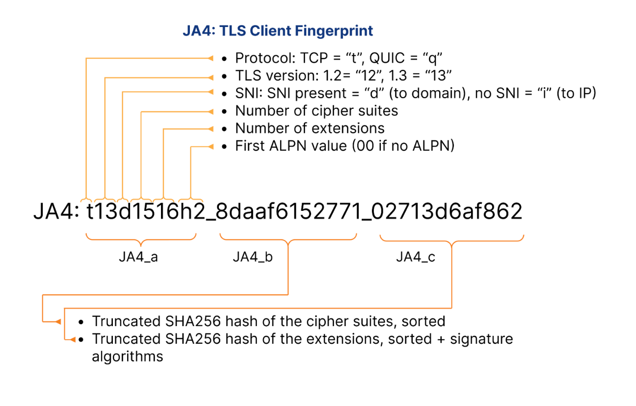
Let’s take a look at specific JA4 fingerprint example, representing the latest version of Google Chrome on Linux:

1. Protocol Identifier (t): Indicates the use of TLS over TCP. This identifier is crucial for determining the underlying protocol, distinguishing it from q for QUIC or d for DTLS.

2. TLS Version (13): Represents TLS version 1.3, confirming that the client is using one of the latest secure protocols. The version number is derived from analyzing the highest version supported in the ClientHello, excluding any GREASE values.

3. SNI Presence (d): The presence of a domain name in the Server Name Indication. This indicates that the client specifies a domain (d), rather than an IP address (i would indicate the absence of SNI).

4. Cipher Suites Count (15): Reflects the total number of cipher suites included in the ClientHello, excluding any GREASE values. It provides insight into the cryptographic options the client is willing to use.

5. Extensions Count (16): Indicates the count of distinct extensions presented by the client in the ClientHello. This measure helps identify the range of functionalities or customizations the client supports.

6. ALPN Values (h2): Represents the Application-Layer Protocol Negotiation protocol, in this case, HTTP/2, which indicates the protocol preferences of the client for optimized web performance.

7. Cipher Hash (8daaf6152771): A truncated SHA256 hash of the list of cipher suites, sorted in hexadecimal order. This unique hash serves as a compact identifier for the client’s cipher suite preferences.

8. Extension Hash (02713d6af862): A truncated SHA256 hash of the sorted list of extensions combined with the list of signature algorithms. This hash provides a unique identifier that helps differentiate clients based on the extensions and signature algorithms they support.

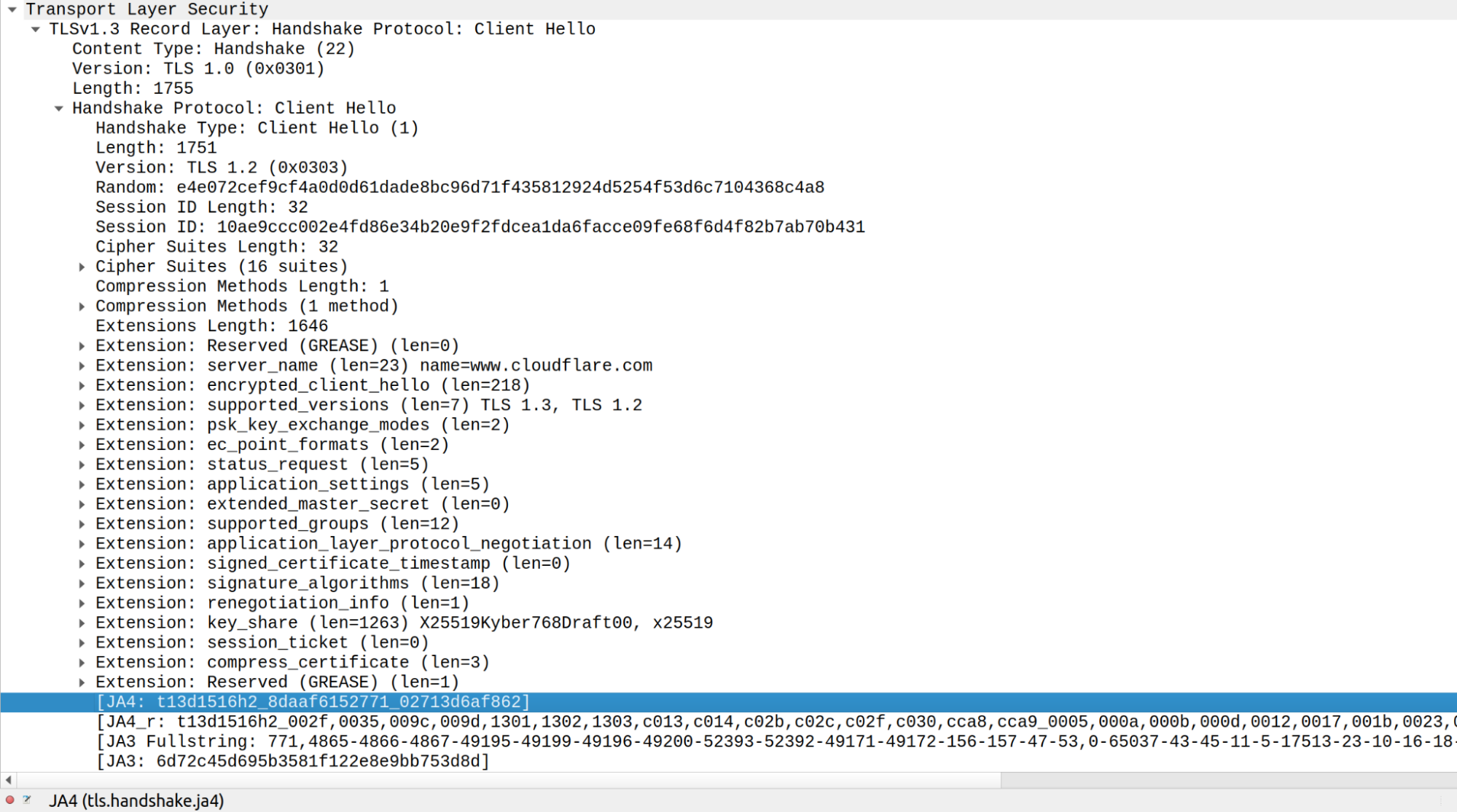
Here is a Wireshark example of TLS ClientHello from the latest Chrome on Linux querying https://www.cloudflare.com:

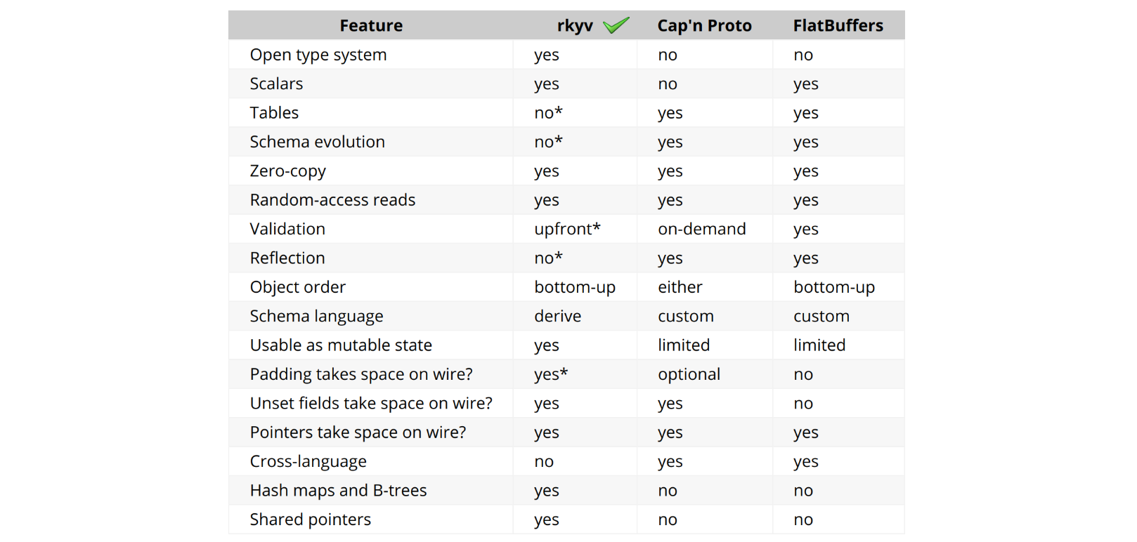
Integrating JA4 support into Cloudflare required rethinking our approach to parsing TLS ClientHello messages, which were previously handled in separate implementations across C, Lua, and Go. Recognizing the need to boost performance and ensure memory safety, we developed a new Rust-based crate, client-hello-parser. This unified parser not only simplifies modifications by centralizing all related logic but also prepares us for future transitions, such as replacing nginx with an upcoming Rust-based service. Additionally, this streamlined parser facilitates the exposure of JA4 fingerprints across our platform, improving the integration with Cloudflare’s firewall rules, Workers, and analytics systems.

Parsing ClientHello

client-hello-parser is an internal Rust crate designed for parsing TLS ClientHello messages. It aims to simplify the process of analyzing TLS traffic by providing a straightforward way to decode and inspect the initial handshake messages sent by clients when establishing TLS connections. This crate efficiently populates a ClientHelloParsed struct with relevant parsed fields, including version 1 and version 2 fingerprints, and JA3 and JA4 hashes, which are essential for network traffic analysis and fingerprinting.

Key benefits of the client-hello-parser library include:

• Optimized memory usage: The library achieves amortized zero heap allocations, verified through extensive testing with the dhat crate to track memory allocations. Utilizing the tiny_vec crate, it begins with stack allocations for small vectors backed by fixed-size arrays, resorting to heap allocations only when these vectors exceed their initial size. This method ensures efficient reuse of all vectors, maintaining amortized zero heap allocations.

• Memory safety: Reinforced by Rust’s robust borrow checker and complemented by extensive fuzzing, which has helped identify and resolve potential security vulnerabilities previously undetected in C implementations.

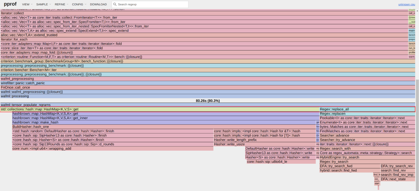
• Ultra-low latency: The parser benefits from using faster_hex for efficient hex encoding/decoding, which utilizes SIMD instructions to speed up processing. The use of Rust iterators also helps in optimizing performance, often allowing the compiler to generate SIMD-optimized assembly code. This efficiency is further enhanced through the use of BigEndianIterator, which allows for efficient streaming-like processing of TLS ClientHello bytes in a single pass.

Parser benchmark results:

client_hello_benchmark/parse/parse-short-502
                        time:   [497.15 ns 497.23 ns 497.33 ns]
                        thrpt:  [2.0107 Melem/s 2.0111 Melem/s 2.0115 Melem/s]
client_hello_benchmark/parse/parse-long-1434
                        time:   [992.82 ns 993.55 ns 994.99 ns]
                        thrpt:  [1.0050 Melem/s 1.0065 Melem/s 1.0072 Melem/s]

The benchmark results demonstrate that the parser efficiently handles different sizes of ClientHello messages, with shorter messages being processed at a rate of approximately 2 million elements per second, and longer messages at around 1 million elements per second, showcasing the effectiveness of SIMD optimizations and Rust’s iterator performance in real-world applications.

Robust testing suite: Includes dozens of real-life TLS ClientHello message examples, with parsed components verified against Wireshark with JA3 and JA4 plugins. Additionally, Cargo fuzzer with memory sanitizer ensures no memory leaks or edge cases leading to core dumps. Backward compatibility tests with the legacy C parser, imported as a dependency and called via FFI, confirm that both parsers yield equivalent results.

Seamless integration with nginx: The crate, compiled as a dynamic library, is linked to the nginx binary, ensuring a smooth transition from the legacy parser to the new Rust-based parser through backwards compatibility tests.

The transition to a new Rust-based parser has enabled the retirement of multiple implementations across different languages (C, Lua, and Go), significantly enhancing performance and parser robustness against edge cases. This shift also facilitates the easier integration of new features and business logic for parsing TLS ClientHello messages, streamlining future expansions and security updates.

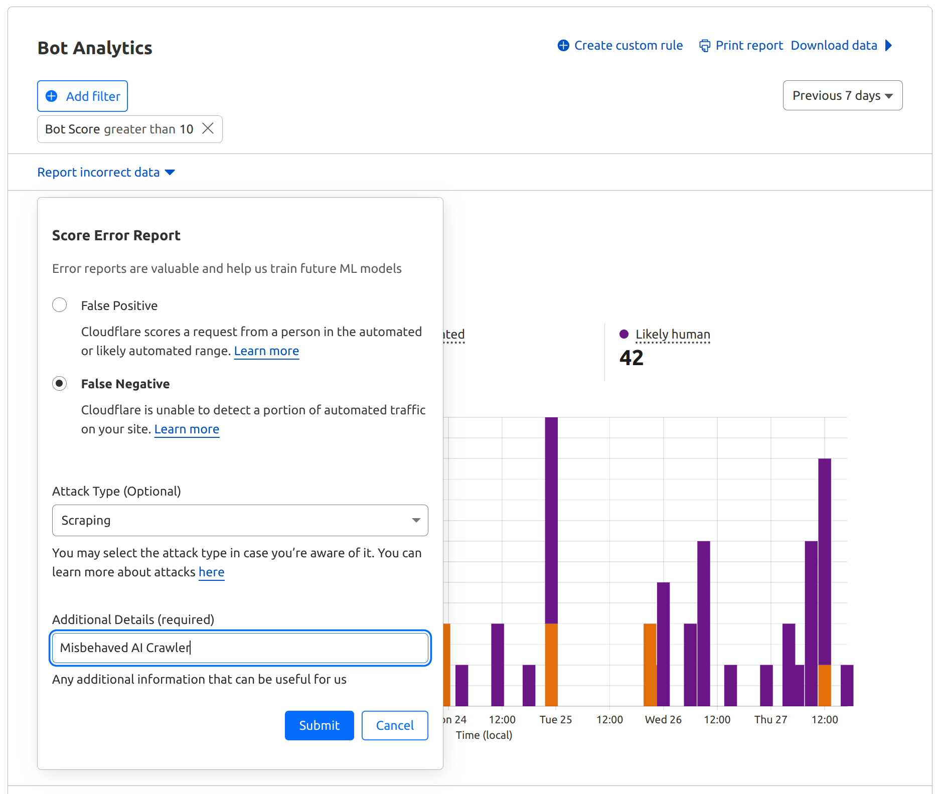
With Cloudflare JA4 fingerprints implemented on our network, we were left with another problem to solve. When JA3 was released, we saw some scenarios where customers were surprised by traffic from a new JA3 fingerprint and blocked it, only to find the fingerprint was a new browser release, or an OS update had caused a change in the fingerprint used by their mobile device. By giving customers just a hash, customers still lack context. We wanted to give our customers the necessary context to help them make informed decisions about the safety of a fingerprint, so they can act quickly and confidently on it. As more of our customers embrace AI, we’ve heard more demand from our customers to break out the signals that power our bot detection. These customers want to run complex models on proprietary data that has to stay in their control, but they want to have Cloudflare’s unique perspective on Internet traffic when they do it. To us, both use cases sounded like the same problem. 

Enter JA4 Signals 

In the ever-evolving landscape of web security, traditional fingerprinting techniques like JA3 and JA4 have proven invaluable for identifying and managing web traffic. However, these methods alone are not sufficient to address the sophisticated tactics employed by malicious agents. Fingerprints can be easily spoofed, they change frequently, and traffic patterns and behaviors are constantly evolving. This is where JA4 Signals come into play, providing a robust and comprehensive approach to traffic analysis.

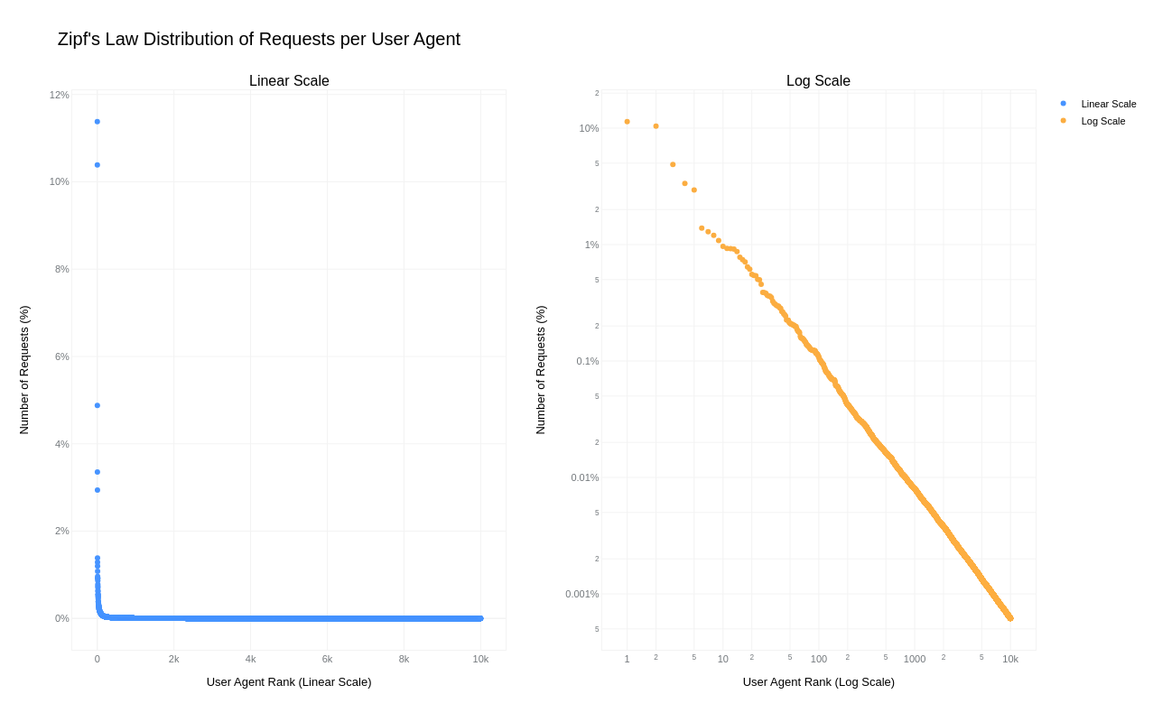
JA4 Signals are inter-request features computed based on the last hour of all traffic that Cloudflare sees globally. On a daily basis, we analyze over 15 million unique JA4 fingerprints generated from more than 500 million user agents and billions of IP addresses. This breadth of data enables JA4 Signals to provide aggregated statistics that offer deeper insights into global traffic patterns – far beyond what single-request or connection fingerprinting can achieve. These signals are crucial for enhancing security measures, whether through simple firewall rules, Workers scripts, or advanced machine learning models.

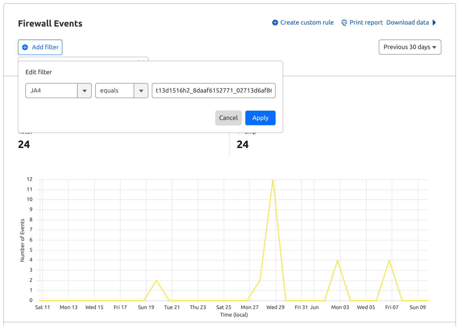
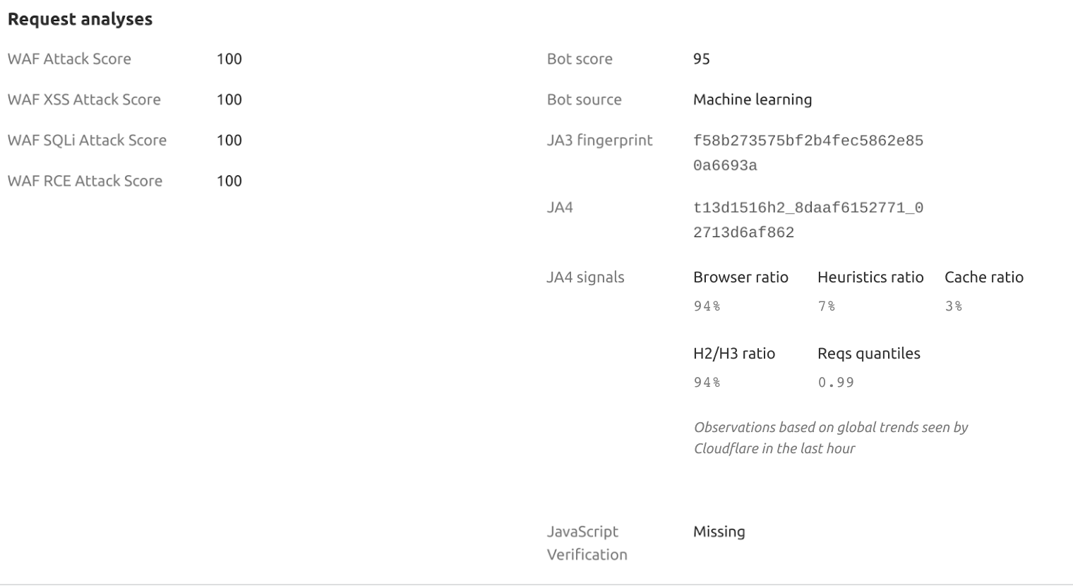
Let’s consider a specific example of JA4 Signals from a Firewall events activity log, which involves the latest version of Chrome:

This example highlights that a particular HTTP request received a Bot Score of 95, suggesting it likely originated from a human user operating a browser rather than an automated program or a bot. Analyzing JA4 Signals in this context provides deeper insight into the behavior of this client (latest Linux Chrome) in comparison to other network clients and their respective JA4 fingerprints. Here are a few examples of the signals our customers can see on any request:

The JA4 fingerprint and JA4 Signals are now available in the Firewall Rules UI, Bot Analytics and Workers. Customers can now use these fields to write custom rules, rate-limiting rules, transform rules, or Workers logic using JA4 fingerprint and JA4 Signals. 

Let’s demonstrate how to use JA4 Signals with the following Worker example. This script processes incoming requests by parsing and categorizing JA4 Signals, providing a clear structure for further analysis or rule application within Cloudflare Workers:

/**
 * Event listener for 'fetch' events. This triggers on every request to the worker.
 */
addEventListener('fetch', event => {
  event.respondWith(handleRequest(event.request))
})

/**
 * Main handler for incoming requests.
 * @param {Request} request - The incoming request object from the fetch event.
 * @returns {Response} A response object with JA4 Signals in JSON format.
 */
async function handleRequest(request) {
  // Safely access the ja4Signals object using optional chaining, which prevents errors if properties are undefined.
  const ja4Signals = request.cf?.botManagement?.ja4Signals || {};

  // Construct the response content, including both the original ja4Signals and the parsed signals.
  const responseContent = {
    ja4Signals: ja4Signals,
    jaSignalsParsed: parseJA4Signals(ja4Signals)
  };

  // Return a JSON response with appropriate headers.
  return new Response(JSON.stringify(responseContent), {
    status: 200,
    headers: {
      "content-type": "application/json;charset=UTF-8"
    }
  })
}

/**
 * Parses the JA4 Signals into categorized groups based on their names.
 * @param {Object} ja4Signals - The JA4 Signals object that may contain various metrics.
 * @returns {Object} An object with categorized JA4 Signals: ratios, ranks, and quantiles.
 */
function parseJA4Signals(ja4Signals) {
  // Define the keys for each category of signals.
  const ratios = ['h2h3_ratio_1h', 'heuristic_ratio_1h', 'browser_ratio_1h', 'cache_ratio_1h'];
  const ranks = ['uas_rank_1h', 'paths_rank_1h', 'reqs_rank_1h', 'ips_rank_1h'];
  const quantiles = ['reqs_quantile_1h', 'ips_quantile_1h'];

  // Return an object with each category containing only the signals that are present.
  return {
    ratios: filterKeys(ja4Signals, ratios),
    ranks: filterKeys(ja4Signals, ranks),
    quantiles: filterKeys(ja4Signals, quantiles)
  };
}

/**
 * Filters the keys in the ja4Signals object that match the list of specified keys and are not undefined.
 * @param {Object} ja4Signals - The JA4 Signals object.
 * @param {Array} keys - An array of keys to filter from the ja4Signals object.
 * @returns {Object} A filtered object containing only the specified keys that are present in ja4Signals.
 */
function filterKeys(ja4Signals, keys) {
  const filtered = {};
  // Iterate over the specified keys and add them to the filtered object if they exist in ja4Signals.
  keys.forEach(key => {
    // Check if the key exists and is not undefined to handle optional presence of each signal.
    if (ja4Signals && ja4Signals[key] !== undefined) {
      filtered[key] = ja4Signals[key];
    }
  });
  return filtered;
}

Benefits of JA4 Signals

• Comprehensive traffic analysis: JA4 Signals aggregate data over an hour to provide a holistic view of traffic patterns. This method enhances the ability to identify emerging threats and abnormal behaviors by analyzing changes over time rather than in isolation.

• Precision in anomaly detection: Leveraging detailed inter-request features, JA4 Signals enable the precise detection of anomalies that may be overlooked by single-request fingerprinting. This leads to more accurate identification of sophisticated cyber threats.

• Globally scalable insights: By synthesizing data at a global scale, JA4 Signals harness the strength of Cloudflare’s network intelligence. This extensive analysis makes the system less susceptible to manipulation and provides a resilient foundation for security protocols.

• Dynamic security enforcement: JA4 Signals can dynamically inform security rules, from simple firewall configurations to complex machine learning algorithms. This adaptability ensures that security measures evolve in tandem with changing traffic patterns and emerging threats.

• Reduction in false positives and negatives: With the detailed insights provided by JA4 Signals, security systems can distinguish between legitimate and malicious traffic more effectively, reducing the occurrence of false positives and negatives and improving overall system reliability.

Conclusion

The introduction of JA4 fingerprint and JA4 Signals marks a significant milestone in advancing Cloudflare’s security offerings, including Bot Management and DDoS protection. These tools not only enhance the robustness of our traffic analysis but also showcase the continuous evolution of our network fingerprinting techniques. The efficiency of computing JA4 fingerprints enables real-time detection and response to emerging threats. Similarly, by leveraging aggregated statistics and inter-request features, JA4 Signals provide deep insights into traffic patterns at speeds measured in microseconds, ensuring that no detail is too small to be captured and analyzed.

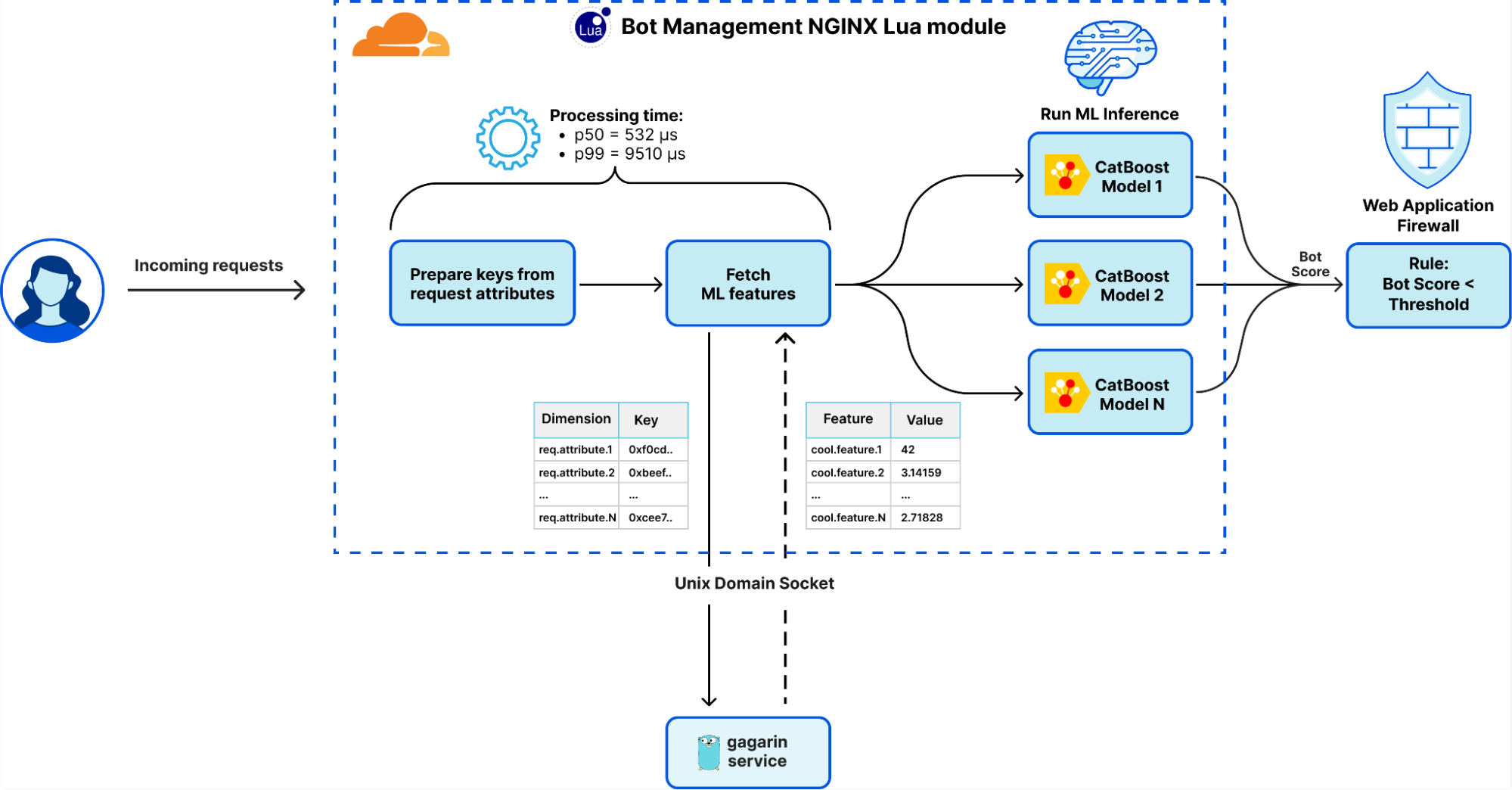
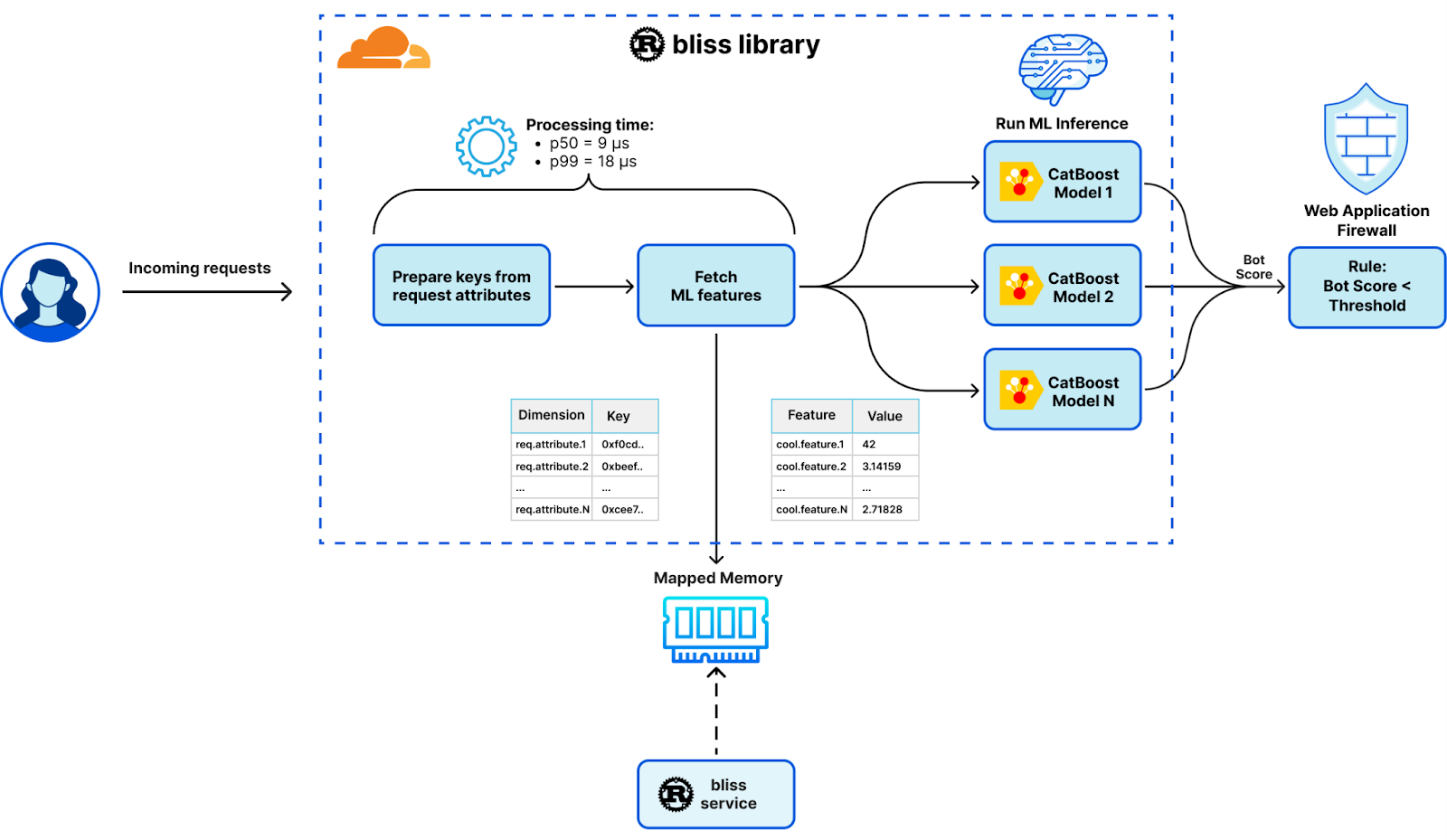
These security features are underpinned by the scalable techniques and open-sourced libraries outlined in “Every request, every microsecond: scalable machine learning at Cloudflare”. This discussion highlights how Cloudflare’s innovations not only analyze vast amounts of data but also transform this analysis into actionable, reliable, and dynamically adaptable security measures.

Any Enterprise business with a bot problem will benefit from Cloudflare’s unique JA4 implementation and our perspective on bot traffic, but customers who run their own internal threat models will also benefit from access to data insights from a network that processes over 50 million requests per second. Please get in touch with us to learn more about our Bot Management offering.

Post Syndicated from Alex Bocharov original https://blog.cloudflare.com/making-waf-ai-models-go-brr

We made our WAF Machine Learning models 5.5x faster, reducing execution time by approximately 82%, from 1519 to 275 microseconds! Read on to find out how we achieved this remarkable improvement.

WAF Attack Score is Cloudflare’s machine learning (ML)-powered layer built on top of our Web Application Firewall (WAF). Its goal is to complement the WAF and detect attack bypasses that we haven’t encountered before. This has proven invaluable in catching zero-day vulnerabilities, like the one detected in Ivanti Connect Secure, before they are publicly disclosed and enhancing our customers’ protection against emerging and unknown threats.

Since its launch in 2022, WAF attack score adoption has grown exponentially, now protecting millions of Internet properties and running real-time inference on tens of millions of requests per second. The feature’s popularity has driven us to seek performance improvements, enabling even broader customer use and enhancing Internet security.

In this post, we will discuss the performance optimizations we’ve implemented for our WAF ML product. We’ll guide you through specific code examples and benchmark numbers, demonstrating how these enhancements have significantly improved our system’s efficiency. Additionally, we’ll share the impressive latency reduction numbers observed after the rollout.

Before diving into the optimizations, let’s take a moment to review the inner workings of the WAF Attack Score, which powers our WAF ML product.

WAF Attack Score system design

Cloudflare’s WAF attack score identifies various traffic types and attack vectors (SQLi, XSS, Command Injection, etc.) based on structural or statistical content properties. Here’s how it works during inference:

1. HTTP Request Content: Start with raw HTTP input.

2. Normalization & Transformation: Standardize and clean the data, applying normalization, content substitutions, and de-duplication.

3. Feature Extraction: Tokenize the transformed content to generate statistical and structural data.

4. Machine Learning Model Inference: Analyze the extracted features with pre-trained models, mapping content representations to classes (e.g., XSS, SQLi or RCE) or scores.

5. Classification Output in WAF: Assign a score to the input, ranging from 1 (likely malicious) to 99 (likely clean), guiding security actions.

Next, we will explore feature extraction and inference optimizations.

Feature extraction optimizations

In the context of the WAF Attack Score ML model, feature extraction or pre-processing is essentially a process of tokenizing the given input and producing a float tensor of 1 x m size:

In our initial pre-processing implementation, this is achieved via a sliding window of 3 bytes over the input with the help of Rust’s std::collections::HashMap to look up the tensor index for a given ngram.

Initial benchmarks

To establish performance baselines, we’ve set up four benchmark cases representing example inputs of various lengths, ranging from 44 to 9482 bytes. Each case exemplifies typical input sizes, including those for a request body, user agent, and URI. We run benchmarks using the Criterion.rs statistics-driven micro-benchmarking tool:

RUSTFLAGS="-C opt-level=3 -C target-cpu=native" cargo criterion

Here are initial numbers for these benchmarks executed on a Linux laptop with a 13th Gen Intel® Core™ i7-13800H processor:

An important observation from these results is that pre-processing time correlates with the length of the input string, with throughput ranging from 28 MiB/s to 36 MiB/s. This suggests that considerable time is spent iterating over longer input strings. Optimizing this part of the process could significantly enhance performance. The dependency of processing time on input size highlights a key area for performance optimization. To validate this, we should examine where the processing time is spent by analyzing flamegraphs created from a 100-second profiling session visualized using pprof:

RUSTFLAGS="-C opt-level=3 -C target-cpu=native" cargo criterion -- --profile-time 100
 
go tool pprof -http=: target/criterion/profile/preprocessing/avg-body-1000/profile.pb

Looking at the pre-processing flamegraph above, it’s clear that most of the time was spent on the following two operations:

Let’s tackle the HashMap lookups first. Lookups are happening inside the tensor_populate_ngrams function, where input is split into windows of 3 bytes representing ngram and then lookup inside two hash maps:

fn tensor_populate_ngrams(tensor: &mut [f32], input: &[u8]) {   
   // Populate the NORM ngrams
   let mut unknown_norm_ngrams = 0;
   let norm_offset = 1;
 
   for s in input.windows(3) {
       match NORM_VOCAB.get(s) {
           Some(pos) => {
               tensor[*pos as usize + norm_offset] += 1.0f32;
           }
           None => {
               unknown_norm_ngrams += 1;
           }
       };
   }
 
   // Populate the SIG ngrams
   let mut unknown_sig_ngrams = 0;
   let sig_offset = norm_offset + NORM_VOCAB.len();
 
   let res = SIG_REGEX.replace_all(&input, b"#");
 
   for s in res.windows(3) {
       match SIG_VOCAB.get(s) {
           Some(pos) => {
               // adding +1 here as the first position will be the unknown_sig_ngrams
               tensor[*pos as usize + sig_offset + 1] += 1.0f32;
           }
           None => {
               unknown_sig_ngrams += 1;
           }
       }
   }
}

So essentially the pre-processing function performs a ton of hash map lookups, the volume of which depends on the size of the input string, e.g. 1469 lookups for the given benchmark case avg-body-1000.

Optimization attempt #1: HashMap → Aho-Corasick

Rust hash maps are generally quite fast. However, when that many lookups are being performed, it’s not very cache friendly.

So can we do better than hash maps, and what should we try first? The answer is the Aho-Corasick library.

This library provides multiple pattern search principally through an implementation of the Aho-Corasick algorithm, which builds a fast finite state machine for executing searches in linear time.

We can also tune Aho-Corasick settings based on this recommendation:

“You might want to use AhoCorasickBuilder::kind to set your searcher to always use AhoCorasickKind::DFA if search speed is critical and memory usage isn’t a concern.”

static ref NORM_VOCAB_AC: AhoCorasick = AhoCorasick::builder().kind(Some(AhoCorasickKind::DFA)).build(&[    
    "abc",
    "def",
    "wuq",
    "ijf",
    "iru",
    "piw",
    "mjw",
    "isn",
    "od ",
    "pro",
    ...
]).unwrap();

Then we use the constructed AhoCorasick dictionary to lookup ngrams using its find_overlapping_iter method:

for mat in NORM_VOCAB_AC.find_overlapping_iter(&input) {
    tensor_input_data[mat.pattern().as_usize() + 1] += 1.0;
}

We ran benchmarks and compared them against the baseline times shown above:

That’s substantially better – Aho-Corasick DFA does wonders.

Optimization attempt #2: Aho-Corasick → match

One would think optimization with Aho-Corasick DFA is enough and that it seems unlikely that anything else can beat it. Yet, we can throw Aho-Corasick away and simply use the Rust match statement and let the compiler do the optimization for us!

#[inline]
const fn norm_vocab_lookup(ngram: &[u8; 3]) -> usize {     
    match ngram {
        b"abc" => 1,
        b"def" => 2,
        b"wuq" => 3,
        b"ijf" => 4,
        b"iru" => 5,
        b"piw" => 6,
        b"mjw" => 7,
        b"isn" => 8,
        b"od " => 9,
        b"pro" => 10,
        ...
        _ => 0,
    }
}```

Here’s how it performs in practice, based on the assembly generated by the Godbolt compiler explorer. The corresponding assembly code efficiently implements this lookup by employing a jump table and byte-wise comparisons to determine the return value based on input sequences, optimizing for quick decisions and minimal branching. Although the example only includes ten ngrams, it’s important to note that in applications like our WAF Attack Score ML models, we deal with thousands of ngrams. This simple match-based approach outshines both HashMap lookups and the Aho-Corasick method.

Switching to match gave us another 7-18% drop in latency, depending on the case.

Optimization attempt #3: Regex → WindowedReplacer

So, what exactly is the purpose of Regex::replace_all in pre-processing? Regex is defined and used like this:

pub static SIG_REGEX: Lazy =
    Lazy::new(|| RegexBuilder::new("[a-z]+").unicode(false).build().unwrap());
    ... 
    let res = SIG_REGEX.replace_all(&input, b"#");
    for s in res.windows(3) {
        tensor[sig_vocab_lookup(s.try_into().unwrap())] += 1.0;
    }

Essentially, all we need is to:

1. Replace every sequence of lowercase letters in the input with a single byte “#”.

2. Iterate over replaced bytes in a windowed fashion with a step of 3 bytes representing an ngram.

3. Look up the ngram index and increment it in the tensor.

This logic seems simple enough that we could implement it more efficiently with a single pass over the input and without any allocations:

type Window = [u8; 3];
type Iter<'a> = Peekable>;

pub struct WindowedReplacer<'a> {
    window: Window,
    input_iter: Iter<'a>,
}

#[inline]
fn is_replaceable(byte: u8) -> bool {
    matches!(byte, b'a'..=b'z')
}

#[inline]
fn next_byte(iter: &mut Iter) -> Option {
    let byte = iter.next().copied()?;
    if is_replaceable(byte) {
        while iter.next_if(|b| is_replaceable(**b)).is_some() {}
        Some(b'#')
    } else {
        Some(byte)
    }
}

impl<'a> WindowedReplacer<'a> {
    pub fn new(input: &'a [u8]) -> Option {
        let mut window: Window = Default::default();
        let mut iter = input.iter().peekable();
        for byte in window.iter_mut().skip(1) {
            *byte = next_byte(&mut iter)?;
        }
        Some(WindowedReplacer {
            window,
            input_iter: iter,
        })
    }
}

impl<'a> Iterator for WindowedReplacer<'a> {
    type Item = Window;

    #[inline]
    fn next(&mut self) -> Option {
        for i in 0..2 {
            self.window[i] = self.window[i + 1];
        }
        let byte = next_byte(&mut self.input_iter)?;
        self.window[2] = byte;
        Some(self.window)
    }
}

By utilizing the WindowedReplacer, we simplify the replacement logic:

if let Some(replacer) = WindowedReplacer::new(&input) {                
    for ngram in replacer.windows(3) {
        tensor[sig_vocab_lookup(ngram.try_into().unwrap())] += 1.0;
    }
}

This new approach not only eliminates the need for allocating additional buffers to store replaced content, but also leverages Rust’s iterator optimizations, which the compiler can more effectively optimize. You can view an example of the assembly output for this new iterator at the provided Godbolt link.

Now let’s benchmark this and compare against the original implementation:

The new letters replacement implementation has doubled the preprocessing speed compared to the previously optimized version using match statements, and it is four to five times faster than the original version!

Optimization attempt #4: Going nuclear with branchless ngram lookups

At this point, 4-5x improvement might seem like a lot and there is no point pursuing any further optimizations. After all, using an ngram lookup with a match statement has beaten the following methods, with benchmarks omitted for brevity:

However, if we look again at the assembly of the norm_vocab_lookup function, it is clear that the execution flow has to perform a bunch of comparisons using cmp instructions. This creates many branches for the CPU to handle, which can lead to branch mispredictions. Branch mispredictions occur when the CPU incorrectly guesses the path of execution, causing delays as it discards partially completed instructions and fetches the correct ones. By reducing or eliminating these branches, we can avoid these mispredictions and improve the efficiency of the lookup process. How can we get rid of those branches when there is a need to look up thousands of unique ngrams?

Since there are only 3 bytes in each ngram, we can build two lookup tables of 256 x 256 x 256 size, storing the ngram tensor index. With this naive approach, our memory requirements will be: 256 x 256 x 256 x 2 x 2 = 64 MB, which seems like a lot.

However, given that we only care about ASCII bytes 0..127, then memory requirements can be lower: 128 x 128 x 128 x 2 x 2 = 8 MB, which is better. However, we will need to check for bytes >= 128, which will introduce a branch again.

So can we do better? Considering that the actual number of distinct byte values used in the ngrams is significantly less than the total possible 256 values, we can reduce memory requirements further by employing the following technique:

1. To avoid the branching caused by comparisons, we use precomputed offset lookup tables. This means instead of comparing each byte of the ngram during each lookup, we precompute the positions of each possible byte in a lookup table. This way, we replace the comparison operations with direct memory accesses, which are much faster and do not involve branching. We build an ngram bytes offsets lookup const array, storing each unique ngram byte offset position multiplied by the number of unique ngram bytes:

const NGRAM_OFFSETS: [[u32; 256]; 3] = [
    [
        // offsets of first byte in ngram
    ],
    [
        // offsets of second byte in ngram
    ],
    [
        // offsets of third byte in ngram
    ],
];

2. Then to obtain the ngram index, we can use this simple const function:

#[inline]
const fn ngram_index(ngram: [u8; 3]) -> usize {
    (NGRAM_OFFSETS[0][ngram[0] as usize]
        + NGRAM_OFFSETS[1][ngram[1] as usize]
        + NGRAM_OFFSETS[2][ngram[2] as usize]) as usize
}

3. To look up the tensor index based on the ngram index, we construct another const array at compile time using a list of all ngrams, where N is the number of unique ngram bytes:

const NGRAM_TENSOR_IDX: [u16; N * N * N] = {
    let mut arr = [0; N * N * N];
    arr[ngram_index(*b"abc")] = 1;
    arr[ngram_index(*b"def")] = 2;
    arr[ngram_index(*b"wuq")] = 3;
    arr[ngram_index(*b"ijf")] = 4;
    arr[ngram_index(*b"iru")] = 5;
    arr[ngram_index(*b"piw")] = 6;
    arr[ngram_index(*b"mjw")] = 7;
    arr[ngram_index(*b"isn")] = 8;
    arr[ngram_index(*b"od ")] = 9;
    ...
    arr
};

4. Finally, to update the tensor based on given ngram, we lookup the ngram index, then the tensor index, and then increment it with help of get_unchecked_mut, which avoids unnecessary (in this case) boundary checks and eliminates another source of branching:

#[inline]
fn update_tensor_with_ngram(tensor: &mut [f32], ngram: [u8; 3]) {
    let ngram_idx = ngram_index(ngram);
    debug_assert!(ngram_idx < NGRAM_TENSOR_IDX.len());
    unsafe {
        let tensor_idx = *NGRAM_TENSOR_IDX.get_unchecked(ngram_idx) as usize;
        debug_assert!(tensor_idx < tensor.len());
        *tensor.get_unchecked_mut(tensor_idx) += 1.0;
    }
}

This logic works effectively, passes correctness tests, and most importantly, it’s completely branchless! Moreover, the memory footprint of used lookup arrays is tiny – just ~500 KiB of memory – which easily fits into modern CPU L2/L3 caches, ensuring that expensive cache misses are rare and performance is optimal.

The last trick we will employ is loop unrolling for ngrams processing. By taking 6 ngrams (corresponding to 8 bytes of the input array) at a time, the compiler can unroll the second loop and auto-vectorize it, leveraging parallel execution to improve performance:

const CHUNK_SIZE: usize = 6;

let chunks_max_offset =
    ((input.len().saturating_sub(2)) / CHUNK_SIZE) * CHUNK_SIZE;
for i in (0..chunks_max_offset).step_by(CHUNK_SIZE) {
    for ngram in input[i..i + CHUNK_SIZE + 2].windows(3) {
        update_tensor_with_ngram(tensor, ngram.try_into().unwrap());
    }
}

Tying up everything together, our final pre-processing benchmarks show the following:

The longer input is, the higher the latency drop will be due to branchless ngram lookups and loop unrolling, ranging from six to twelve times faster than baseline implementation.

After trying various optimizations, the final version of pre-processing retains optimization attempts 3 and 4, using branchless ngram lookup with offset tables and a single-pass non-allocating replacement iterator.

There are potentially more CPU cycles left on the table, and techniques like memory pre-fetching and manual SIMD intrinsics could speed this up a bit further. However, let’s now switch gears into looking at inference latency a bit closer.

Model inference optimizations

Initial benchmarks

Let’s have a look at original performance numbers of the WAF Attack Score ML model, which uses TensorFlow Lite 2.6.0:

Model inference is actually independent of the original input length, as inputs are transformed into tensors of predetermined size during the pre-processing phase, which we optimized above. From now on, we will refer to a singular inference time when benchmarking our optimizations.

Digging deeper with profiler, we observed that most of the time is spent on the following operations:

The most expensive operation is matrix multiplication, which boils down to iteration within three nested loops:

void PortableMatrixBatchVectorMultiplyAccumulate(const float* matrix,
                                                 int m_rows, int m_cols,
                                                 const float* vector,
                                                 int n_batch, float* result) {
  float* result_in_batch = result;
  for (int b = 0; b < n_batch; b++) {
    const float* matrix_ptr = matrix;
    for (int r = 0; r < m_rows; r++) {
      float dot_prod = 0.0f;
      const float* vector_in_batch = vector + b * m_cols;
      for (int c = 0; c < m_cols; c++) {
        dot_prod += *matrix_ptr++ * *vector_in_batch++;
      }
      *result_in_batch += dot_prod;
     ++result_in_batch;
    }
  }
}

This doesn’t look very efficient and many blogs and research papers have been written on how matrix multiplication can be optimized, which basically boils down to:

• Blocking: Divide matrices into smaller blocks that fit into the cache, improving cache reuse and reducing memory access latency.

• Vectorization: Use SIMD instructions to process multiple data points in parallel, enhancing efficiency with vector registers.

• Loop Unrolling: Reduce loop control overhead and increase parallelism by executing multiple loop iterations simultaneously.

To gain a better understanding of how these techniques work, we recommend watching this video, which brilliantly depicts the process of matrix multiplication:

Tensorflow Lite with AVX2

TensorFlow Lite does, in fact, support SIMD matrix multiplication – we just need to enable it and re-compile the TensorFlow Lite library:

if [[ "$(uname -m)" == x86_64* ]]; then
    # On x86_64 target x86-64-v3 CPU to enable AVX2 and FMA.
    arguments+=("--copt=-march=x86-64-v3")
fi

After running profiler again using the SIMD-optimized TensorFlow Lite library:

Top operations as per profiler output:

Matrix multiplication now uses AVX2 instructions, which uses blocks of 8×8 to multiply and accumulate the multiplication result.

Proportionally, matrix multiplication and quantization operations take a similar time share when compared to non-SIMD version, however in absolute numbers, it’s almost twice as fast when SIMD optimizations are enabled:

Quite a nice performance boost just from a few lines of build config change!

Tensorflow Lite with XNNPACK

Tensorflow Lite comes with a useful benchmarking tool called benchmark_model, which also has a built-in profiler.

The tool can be built locally using the command:

bazel build -j 4 --copt=-march=native -c opt tensorflow/lite/tools/benchmark:benchmark_model

After building, benchmarks were run with different settings:

Tensorflow Lite with XNNPACK enabled emerges as a leader, achieving ~50% latency reduction, when compared to the original Tensorflow Lite implementation.

More technical details about XNNPACK can be found in these blog posts:

• Profiling XNNPACK with TFLite

• Faster Dynamically Quantized Inference with XNNPack

Re-running benchmarks with XNNPack enabled, we get the following results:

By upgrading TensorFlow Lite from 2.6.0 to 2.16.1 and enabling SIMD optimizations along with the XNNPack, we were able to decrease WAF ML model inference time more than four-fold, achieving a 77.17% reduction.

Caching inference result

While making code faster through pre-processing and inference optimizations is great, it’s even better when code doesn’t need to run at all. This is where caching comes in. Amdahl’s Law suggests that optimizing only parts of a program has diminishing returns. By avoiding redundant executions with caching, we can achieve significant performance gains beyond the limitations of traditional code optimization.

A simple key-value cache would quickly occupy all available memory on the server due to the high cardinality of URLs, HTTP headers, and HTTP bodies. However, because “everything on the Internet has an L-shape” or more specifically, follows a Zipf’s law distribution, we can optimize our caching strategy.

Zipf‘s law states that in many natural datasets, the frequency of any item is inversely proportional to its rank in the frequency table. In other words, a few items are extremely common, while the majority are rare. By analyzing our request data, we found that URLs, HTTP headers, and even HTTP bodies follow this distribution. For example, here is the user agent header frequency distribution against its rank:

By caching the top-N most frequently occurring inputs and their corresponding inference results, we can ensure that both pre-processing and inference are skipped for the majority of requests. This is where the Least Recently Used (LRU) cache comes in – frequently used items stay hot in the cache, while the least recently used ones are evicted.

We use lua-resty-mlcache as our caching solution, allowing us to share cached inference results between different Nginx workers via a shared memory dictionary. The LRU cache effectively exploits the space-time trade-off, where we trade a small amount of memory for significant CPU time savings.

This approach enables us to achieve a ~70% cache hit ratio, significantly reducing latency further, as we will analyze in the final section below.

Optimization results

The optimizations discussed in this post were rolled out in several phases to ensure system correctness and stability.

First, we enabled SIMD optimizations for TensorFlow Lite, which reduced WAF ML total execution time by approximately 41.80%, decreasing from 1519 ➔ 884 μs on average.

Next, we upgraded TensorFlow Lite from version 2.6.0 to 2.16.1, enabled XNNPack, and implemented pre-processing optimizations. This further reduced WAF ML total execution time by ~40.77%, bringing it down from 932 ➔ 552 μs on average. The initial average time of 932 μs was slightly higher than the previous 884 μs due to the increased number of customers using this feature and the months that passed between changes.

Lastly, we introduced LRU caching, which led to an additional reduction in WAF ML total execution time by ~50.18%, from 552 ➔ 275 μs on average.

Overall, we cut WAF ML execution time by ~81.90%, decreasing from 1519 ➔ 275 μs, or 5.5x faster!

To illustrate the significance of this: with Cloudflare’s average rate of 9.5 million requests per second passing through WAF ML, saving 1244 microseconds per request equates to saving ~32 years of processing time every single day! That’s in addition to the savings of 523 microseconds per request or 65 years of processing time per day demonstrated last year in our Every request, every microsecond: scalable machine learning at Cloudflare post about our Bot Management product.

Conclusion

We hope you enjoyed reading about how we made our WAF ML models go brrr, just as much as we enjoyed implementing these optimizations to bring scalable WAF ML to more customers on a truly global scale.

Looking ahead, we are developing even more sophisticated ML security models. These advancements aim to bring our WAF and Bot Management products to the next level, making them even more useful and effective for our customers.