Post Syndicated from Jeremy Ber original https://aws.amazon.com/blogs/big-data/in-place-version-upgrades-for-applications-on-amazon-managed-service-for-apache-flink-now-supported/
For existing users of Amazon Managed Service for Apache Flink who are excited about the recent announcement of support for Apache Flink runtime version 1.18, you can now statefully migrate your existing applications that use older versions of Apache Flink to a more recent version, including Apache Flink version 1.18. With in-place version upgrades, upgrading your application runtime version can be achieved simply, statefully, and without incurring data loss or adding additional orchestration to your workload.
Apache Flink is an open source distributed processing engine, offering powerful programming interfaces for both stream and batch processing, with first-class support for stateful processing and event time semantics. Apache Flink supports multiple programming languages, Java, Python, Scala, SQL, and multiple APIs with different level of abstraction, which can be used interchangeably in the same application.
Managed Service for Apache Flink is a fully managed, serverless experience in running Apache Flink applications, and now supports Apache Flink 1.18.1, the latest released version of Apache Flink at the time of writing.
In this post, we explore in-place version upgrades, a new feature offered by Managed Service for Apache Flink. We provide guidance on getting started and offer detailed insights into the feature. Later, we deep dive into how the feature works and some sample use cases.
This post is complemented by an accompanying video on in-place version upgrades, and code samples to follow along.
Use the latest features within Apache Flink without losing state
With each new release of Apache Flink, we observe continuous improvements across all aspects of the stateful processing engine, from connector support to API enhancements, language support, checkpoint and fault tolerance mechanisms, data format compatibility, state storage optimization, and various other enhancements. To learn more about the features supported in each Apache Flink version, you can consult the Apache Flink blog, which discusses at length each of the Flink Improvement Proposals (FLIPs) incorporated into each of the versioned releases. For the most recent version of Apache Flink supported on Managed Service for Apache Flink, we have curated some notable additions to the framework you can now use.
With the release of in-place version upgrades, you can now upgrade to any version of Apache Flink within the same application, retaining state in between upgrades. This feature is also useful for applications that don’t require retaining state, because it makes the runtime upgrade process seamless. You don’t need to create a new application in order to upgrade in-place. In addition, logs, metrics, application tags, application configurations, VPCs, and other settings are retained between version upgrades. Any existing automation or continuous integration and continuous delivery (CI/CD) pipelines built around your existing applications don’t require changes post-upgrade.
In the following sections, we share best practices and considerations while upgrading your applications.
Make sure your application code runs successfully in the latest version
Before upgrading to a newer runtime version of Apache Flink on Managed Service for Apache Flink, you need to update your application code, version dependencies, and client configurations to match the target runtime version due to potential inconsistencies between application versions for certain Apache Flink APIs or connectors. Additionally, there may have been changes within the existing Apache Flink interface between versions that will require updating. Refer to Upgrading Applications and Flink Versions for more information about how to avoid any unexpected inconsistencies.
The next recommended step is to test your application locally with the newly upgraded Apache Flink runtime. Make sure the correct version is specified in your build file for each of your dependencies. This includes the Apache Flink runtime and API and recommended connectors for the new Apache Flink runtime. Running your application with realistic data and throughput profiles can prevent issues with code compatibility and API changes prior to deploying onto Managed Service for Apache Flink.
After you have sufficiently tested your application with the new runtime version, you can begin the upgrade process. Refer to General best practices and recommendations for more details on how to test the upgrade process itself.
It is strongly recommended to test your upgrade path on a non-production environment to avoid service interruptions to your end-users.
Build your application JAR and upload to Amazon S3
You can build your Maven projects by following the instructions in How to use Maven to configure your project. If you’re using Gradle, refer to How to use Gradle to configure your project. For Python applications, refer to the GitHub repo for packaging instructions.
Next, you can upload this newly created artifact to Amazon Simple Storage Service (Amazon S3). It is strongly recommended to upload this artifact with a different name or different location than the existing running application artifact to allow for rolling back the application should issues arise. Use the following code:
The following is an example:
Take a snapshot of the current running application
It is recommended to take a snapshot of your current running application state prior to starting the upgrade process. This enables you to roll back your application statefully if issues occur during or after your upgrade. Even if your applications don’t use state directly in the case of windows, process functions, or similar, they may still use Apache Flink state in the case of a source like Apache Kafka or Amazon Kinesis, remembering the position in the topic or shard it last left off before restarting. This helps prevent duplicate data entering the stream processing application.
Some things to keep in mind:
- Stateful downgrades are not compatible and will not be accepted due to snapshot incompatibility.
- Validation of the state snapshot compatibility happens when the application attempts to start in the new runtime version. This will happen automatically for applications in
RUNNINGmode, but for applications that are upgraded inREADYstate, the compatibility check will only happen when the application starts by calling theRunApplicationaction. - Stateful upgrades from an older version of Apache Flink to a newer version are generally compatible with rare exceptions. Make sure your current Flink version is snapshot-compatible with the target Flink version by consulting the Apache Flink state compatibility table.
Begin the upgrade of a running application
After you have tested your new application, uploaded the artifacts to Amazon S3, and taken a snapshot of the current application, you are now ready to begin upgrading your application. You can upgrade your applications using the UpdateApplication action:
This command invokes several processes to perform the upgrade:
- Compatibility check – The API will check if your existing snapshot is compatible with the target runtime version. If compatible, your application will transition into
UPDATINGstatus, otherwise your upgrade will be rejected and resume processing data with unaffected application. - Restore from latest snapshot with new code – The application will then attempt to start using the most recent snapshot. If the application starts running and behavior appears in-line with expectations, no further action is needed.
- Manual intervention may be required – Keep a close watch on your application throughout the upgrade process. If there are unexpected restarts, failures, or issues of any kind, it is recommended to roll back to the previous version of your application.
When the application is in RUNNING status in the new application version, it is still recommended to closely monitor the application for any unexpected behavior, state incompatibility, restarts, or anything else related to performance.
Unexpected issues while upgrading
In the event of encountering any issues with your application following the upgrade, you retain the ability to roll back your running application to the previous application version. This is the recommended approach if your application is unhealthy or unable to take checkpoints or snapshots while upgrading. Additionally, it’s recommended to roll back if you observe unexpected behavior out of the application.
There are several scenarios to be aware of when upgrading that may require a rollback:
- An app stuck in
UPDATINGstate for any reason can use the RollbackApplication action to trigger a rollback to the original runtime - If an application successfully upgrades to a newer Apache Flink runtime and switches to
RUNNINGstatus, but exhibits unexpected behavior, it can use theRollbackApplicationfunction to revert back to the prior application version - An application fails via the
UpgradeApplicationcommand, which will result in the upgrade not taking place to begin with
Edge cases
There are several known issues you may face when upgrading your Apache Flink versions on Managed Service for Apache Flink. Refer to Precautions and known issues for more details to see if they apply to your specific applications. In this section, we walk through one such use case of state incompatibility.
Consider a scenario where you have an Apache Flink application currently running on runtime version 1.11, using the Amazon Kinesis Data Streams connector for data retrieval. Due to notable alterations made to the Kinesis Data Streams connector across various Apache Flink runtime versions, transitioning directly from 1.11 to 1.13 or higher while preserving state may pose difficulties. Notably, there are disparities in the software packages employed: Amazon Kinesis Connector vs. Apache Kinesis Connector. Consequently, this difference will lead to complications when attempting to restore state from older snapshots.
For this specific scenario, it’s recommended to use the Amazon Kinesis Connector Flink State Migrator, a tool to help migrate Kinesis Data Streams connectors to Apache Kinesis Data Stream connectors without losing state in the source operator.
For illustrative purposes, let’s walk through the code to upgrade the application:
This command will issue an update command and run all compatibility checks. Additionally, the application may even start, displaying the RUNNING status on the Managed Service for Apache Flink console and API.
However, with a closer inspection into your Apache Flink Dashboard to view the fullRestart metrics and application behavior, you may find that the application has failed to start due to the state from the 1.11 version of the application’s state being incompatible with the new application due changing the connector as described previously.
You can roll back to the previous running version, restoring from the successfully taken snapshot, as shown in the following code. If the application has no snapshots, Managed Service for Apache Flink will reject the rollback request.
After issuing this command, your application should be running again in the original runtime without any data loss, thanks to the application snapshot that was taken previously.
This scenario is meant as a precaution, and a recommendation that you should test your application upgrades in a lower environment prior to production. For more details about the upgrade process, along with general best practices and recommendations, refer to In-place version upgrades for Apache Flink.
Conclusion
In this post, we covered the upgrade path for existing Apache Flink applications running on Managed Service for Apache Flink and how you should make modifications to your application code, dependencies, and application JAR prior to upgrading. We also recommended taking snapshots of your application prior to the upgrade process, along with testing your upgrade path in a lower environment. We hope you found this post helpful and that it provides valuable insights into upgrading your applications seamlessly.
To learn more about the new in-place version upgrade feature from Managed Service for Apache Flink, refer to In-place version upgrades for Apache Flink, the how-to video, the GitHub repo, and Upgrading Applications and Flink Versions.
About the Authors

Jeremy Ber boasts over a decade of expertise in stream processing, with the last four years dedicated to AWS as a Streaming Specialist Solutions Architect. With a robust ten-year career background, Jeremy’s commitment to stream processing, notably Apache Flink, underscores his professional endeavors. Transitioning from Software Engineer to his current role, Jeremy prioritizes assisting customers in resolving complex challenges with precision. Whether elucidating Amazon Managed Streaming for Apache Kafka (Amazon MSK) or navigating AWS’s Managed Service for Apache Flink, Jeremy’s proficiency and dedication ensure efficient problem-solving. In his professional approach, excellence is maintained through collaboration and innovation.

Krzysztof Dziolak is Sr. Software Engineer on Amazon Managed Service for Apache Flink. He works with product team and customers to make streaming solutions more accessible to engineering community.


 Lorenzo Nicora works as Senior Streaming Solution Architect at AWS, helping customers across EMEA. He has been building cloud-native, data-intensive systems for over 25 years, working in the finance industry both through consultancies and for FinTech product companies. He has leveraged open-source technologies extensively and contributed to several projects, including Apache Flink.


 Jeremy Ber has been working in the telemetry data space for the past 9 years as a Software Engineer, Machine Learning Engineer, and most recently a Data Engineer. At AWS, he is a Streaming Specialist Solutions Architect, supporting both Amazon Managed Streaming for Apache Kafka (Amazon MSK) and AWS’s managed offering for Apache Flink.
 Deepthi Mohan is a Principal Product Manager for Amazon Kinesis Data Analytics, AWS’s managed offering for Apache Flink.
 Gaurav Rele is a Data Scientist at the Amazon ML Solution Lab, where he works with AWS customers across different verticals to accelerate their use of machine learning and AWS Cloud services to solve their business challenges.


 Pratik Patel is a Sr Technical Account Manager and streaming analytics specialist. He works with AWS customers and provides ongoing support and technical guidance to help plan and build solutions using best practices, and proactively helps keep customer’s AWS environments operationally healthy.
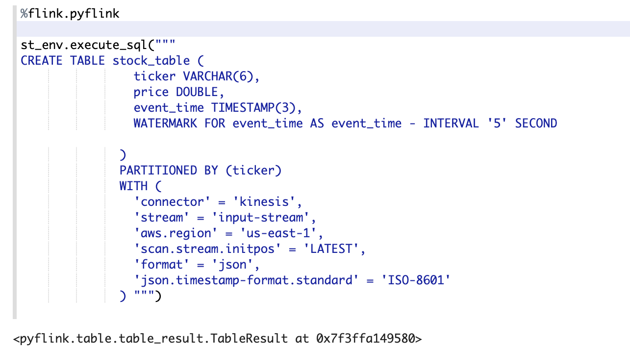


 Jeremy Ber has been working in the telemetry data space for the past 5 years as a Software Engineer, Machine Learning Engineer, and most recently a Data Engineer. In the past, Jeremy has supported and built systems that stream in terabytes of data per day, and process complex machine learning algorithms in real time. At AWS, he is a Solutions Architect Streaming Specialist supporting both Managed Streaming for Kafka (Amazon MSK) and Amazon Kinesis.