All posts by Raks Khare

Amazon Redshift Python user-defined functions will reach end of support after June 30, 2026

Post Syndicated from Raks Khare original https://aws.amazon.com/blogs/big-data/amazon-redshift-python-user-defined-functions-will-reach-end-of-support-after-june-30-2026/

The Amazon Redshift integration with AWS Lambda provides the capability to create Amazon Redshift Lambda user-defined functions (UDFs). This capability delivers flexibility, enhanced integrations, and security for functions defined in Lambda that can be run through SQL queries. Amazon Redshift Lambda UDFs offer many advantages:

  • Enhanced integration – You can connect to external services or APIs from within your UDF logic, enabling richer data enrichment and operational workflows.
  • Multiple Python runtimes – Lambda UDFs benefit from Lambda function support for multiple Python runtimes depending on specific use cases. In addition, the new versions and security patches are available within a month of their official release.
  • Independent scaling – Lambda UDFs use Lambda compute resources, so heavy compute or memory-intensive tasks don’t impact query performance or resource concurrency within Amazon Redshift.
  • Isolation and security – You can isolate custom code execution in a separate service boundary. This simplifies maintenance, monitoring, budgeting, and permission management.

Because Lambda UDFs provide these significant advantages in integration, flexibility, scalability, and security, we will be ending support for Python UDFs in Amazon Redshift. We recommend that you migrate your existing Python UDFs to Lambda UDFs by June 30, 2026.

  • October 30, 2025 – Creation of new Python UDFs will no longer be supported (existing functions can still be invoked)
  • June 30, 2026 – Execution of existing Python UDFs will be suspended

In this post, we walk you through how to migrate your existing Python UDFs to Lambda UDFs, set up monitoring and cost evaluations, and review key considerations for a smooth transition.

Solution overview

You can create UDFs for tasks such as tokenization, encryption and decryption, or data science functionality like the Levenshtein distance calculation. For this post, we provide examples for customers who have Python UDFs in place, demonstrating how to replace them with Lambda UDFs.

The Levenshtein function, also known as the Levenshtein distance or edit distance, is a string metric used to measure the difference between two sequences of characters. Although this functionality was previously implemented using Python UDFs using the Python library in Amazon Redshift, Lambda provides a more efficient and scalable solution. This post demonstrates how to migrate from Python UDFs to Lambda UDFs for calculating Levenshtein distances.

Prerequisites

You must have the following:

Prepare the data

To set up our use case, complete the following steps:

  1. On the Amazon Redshift console, choose Query editor v2 under Explorer in the navigation pane.
  2. Connect to your Redshift data warehouse.
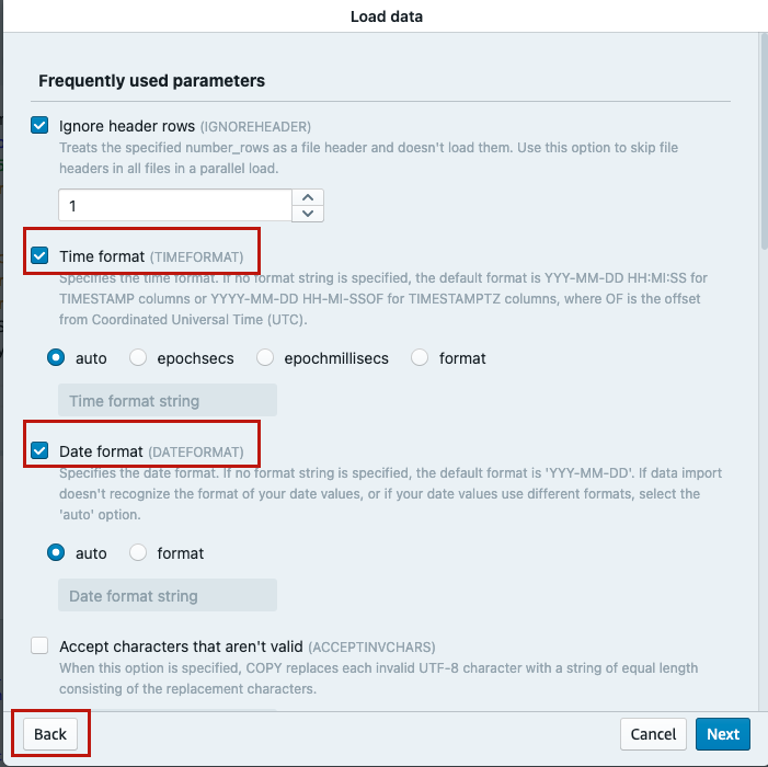
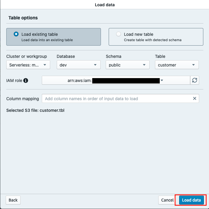
  3. Create a table and load data. The following query loads 30,000,000 rows in the customer table:
DROP TABLE IF EXISTS customer;
CREATE TABLE customer
(
c_customer_sk int4 not null ,
c_customer_id char(16) not null ,
c_current_cdemo_sk int4 ,
c_current_hdemo_sk int4 ,
c_current_addr_sk int4 ,
c_first_shipto_date_sk int4 ,
c_first_sales_date_sk int4 ,
c_salutation char(10) ,
c_first_name char(20) ,
c_last_name char(30) ,
c_preferred_cust_flag char(1) ,
c_birth_day int4 ,
c_birth_month int4 ,
c_birth_year int4 ,
c_birth_country varchar(20) ,
c_login char(13) ,
c_email_address char(50) ,
c_last_review_date_sk int4 ,
primary key (c_customer_sk)
) distkey(c_customer_sk);

COPY customer from 's3://redshift-downloads/TPC-DS/2.13/3TB/customer/'
IAM_ROLE default gzip delimiter '|' EMPTYASNULL REGION 'us-east-1';

Identify existing Python UDFs

Run the following script to list existing Python UDFs:

SELECT 
    p.proname, 
    p.pronargs, 
    t.typname, 
    n.nspname, 
    l.lanname, 
    pg_get_functiondef(p.oid) 
FROM 
    pg_proc p, 
    pg_language l, 
    pg_type t, 
    pg_namespace n
WHERE 
    p.prolang = l.oid
    and p.prorettype = t.oid
    and l.lanname = 'plpythonu'
    and p.pronamespace = n.oid
    and nspname not in ('pg_catalog', 'information_schema')
ORDER BY 
    proname;

The following is our existing Python UDF definition for Levenshtein distance:

create or replace function fn_levenshtein_distance(a varchar, b varchar) returns integer as
$$

def levenshtein_distance(a, len_a, b, len_b):
    d = [[0] * (len_b + 1) for i in range(len_a + 1)]  

    for i in range(1, len_a + 1):
        d[i][0] = i

    for j in range(1, len_b + 1):
        d[0][j] = j
    
    for j in range(1, len_b + 1):
        for i in range(1, len_a + 1):
            if a[i - 1] == b[j - 1]:
                cost = 0
            else:
                cost = 1
            d[i][j] = min(d[i - 1][j] + 1,      # deletion
                          d[i][j - 1] + 1,      # insertion
                          d[i - 1][j - 1] + cost) # substitution   

    return d[len_a][len_b]

def distance(a, b):
    len_a, len_b = len(a), len(b)
    if len_a == len_b:
        return 0
    elif len_a == 0:
        return len_b
    elif len_b == 0:
        return len_a
    else:
        return levenshtein_distance(a, len_a, b, len_b)

return distance(a, b)
$$ immutable;

Convert the Python UDF function to a Lambda UDF

You can simplify converting your Python UDF to a Lambda UDF using Amazon Q Developer, a generative AI-powered assistant. It handles code transformation, packaging, and integration logic, accelerating migration and improving scalability. Integrated with popular developer tools like VS Code, JetBrains, and others, Amazon Q streamlines workflows so teams can modernize analytics using serverless architectures with minimal effort.

Amazon Q Developer code suggestions are based on large language models (LLMs) trained on billions of lines of code, including open source and Amazon code. Always review a code suggestion before accepting it, and you might need to edit it to make sure that it does exactly what you intended.

Convert @python-udf.py Redshift Python UDF to Redshift Lambda UDF which batch processes data in the arguments array in a loop and returns json dump at the end. Refer to @lambda-context.py for reference and additional guidance on Lambda UDF.

Create a Lambda function

Complete the following steps to create a Lambda function:

  1. On the Lambda console, choose Functions in the navigation pane.
  2. Choose Create function.
  3. Choose Author from scratch.
  4. For Function name, enter a custom name (for example, levenshtein_distance_func).
  5. For Runtime, choose your code environment. (The examples in this post are compatible with Python 3.12.)
  6. For Architecture, select your system architecture. (The examples in this post are compatible with x86_64.)

  1. For Execution role, select Create a new role with basic Lambda permissions.

  1. Choose Create function.
  2. Choose Code and add the following code:
import json

def lambda_handler(event, context):
    t1 = event['arguments']
    resp = [None]*len(t1)

    for i, x in enumerate(t1):
        if x[0] is not None and x[1] is not None:
            resp[i] = distance(x[0], x[1])

    ret = dict()
    ret['results'] = resp
    return json.dumps(ret)

def levenshtein_distance(a, len_a, b, len_b):
    d = [[0] * (len_b + 1) for i in range(len_a + 1)]  

    for i in range(1, len_a + 1):
        d[i][0] = i

    for j in range(1, len_b + 1):
        d[0][j] = j
    
    for j in range(1, len_b + 1):
        for i in range(1, len_a + 1):
            if a[i - 1] == b[j - 1]:
                cost = 0
            else:
                cost = 1
            d[i][j] = min(d[i - 1][j] + 1,      # deletion
                          d[i][j - 1] + 1,      # insertion
                          d[i - 1][j - 1] + cost) # substitution   

    return d[len_a][len_b]

def distance(a, b):
    len_a, len_b = len(a), len(b)
    if len_a == len_b and a == b:
        return 0
    elif len_a == 0:
        return len_b
    elif len_b == 0:
        return len_a
    else:
        return levenshtein_distance(a, len_a, b, len_b)
  1. Choose configuration and update Timeout to 1 minute.

You can modify memory to optimize performance. To learn more, see Optimizing Levenshtein User-Defined Function in Amazon Redshift.

Create an Amazon Redshift IAM role

To allow your Amazon Redshift cluster to invoke the Lambda function, you must set up proper IAM permissions. Complete the following steps:

  1. Identify the IAM role associated with your Amazon Redshift cluster. If you don’t have one, create a new IAM role for Amazon Redshift.
  2. Add the following IAM policy to this role, providing your AWS Region and AWS account number:
{
"Version": "2012-10-17",
"Statement": [
{
"Effect": "Allow",
"Action": "lambda:InvokeFunction",
"Resource": "arn:aws:lambda:<REGION>:<AWS account>:function:levenshtein_distance_func"
}
]
}

Create a Lambda UDF

Run following script to create your Lambda UDF:

CREATE or REPLACE EXTERNAL FUNCTION 
fn_lambda_levenshtein_distance(a varchar, b varchar) returns int
lambda 'levenshtein_distance_func' IAM_ROLE default 
STABLE
;

Test the solution

To test the solution, run the following script using the Python UDF:

SELECT c_customer_sk, c_customer_id, fn_levenshtein_distance(c_first_name, c_last_name) as distance
FROM customer
WHERE c_customer_sk in (1,2,3,4,5,31);

The following table shows our output.

Run the same script using the Lambda UDF:

SELECT c_customer_sk, c_customer_id, fn_lambda_levenshtein_distance(c_first_name, c_last_name) as distance
FROM customer
WHERE c_customer_sk in (1,2,3,4,5,31);

The results of both UDFs match.

Replace the Python UDF with the Lambda UDF

You can use the following steps in preproduction for testing:

  1. Revoke access for the Python UDF:
REVOKE execute on function fn_levenshtein_distance(varchar, varchar) from <group_name> or <role_name>
  1. Grant access to the Lambda UDF:
grant execute on function fn_lambda_levenshtein_distance(varchar, varchar) to <group_name> or <role_name>
  1. After full testing of the Lambda UDF has been performed, you can drop the Python UDF.
  2. Rename the Lambda UDF fn_lambda_levenshtein_distance to fn_levenshtein_distance so the end-user and application code doesn’t need to change:
ALTER FUNCTION fn_lambda_levenshtein_distance(varchar, varchar)
     RENAME TO fn_levenshtein_distance;
  1. Validate with the following query:
SELECT c_customer_sk, c_customer_id, fn_levenshtein_distance(c_first_name, c_last_name) as distance
FROM customer
WHERE c_customer_sk in (1,2,3,4,5,31);

Cost evaluation

To evaluate the cost of the Lambda UDF, complete the following steps:

  1. Run the following script to create a table using a SELECT query, which uses the Lambda UDF:
DROP TABLE IF EXISTS customer_lambda;
CREATE TABLE customer_lambda as 
SELECT c_customer_sk, c_customer_id, fn_levenshtein_distance(c_first_name, c_last_name) as distance
FROM customer;

You can inspect the query logs using CloudWatch Log Insights.

  1. On the CloudWatch console, choose Logs in the navigation pane, then choose Log Insights.
  2. Filter by the Lambda UDF and use the following query to identify the number of Lambda invocations.
fields @timestamp, @message, @logStream, @log
| filter @message like /^REPORT/
| sort @timestamp desc
| limit 10000

  1. Use following query to find the cost of the Lambda UDF for the specific duration you selected:
parse @message /Duration:\s*(?<@duration_ms>\d+\.\d+)\s*ms\s*Billed\s*Duration:\s*(?<@billed_duration_ms>\d+)\s*ms\s*Memory\s*Size:\s*(?<@memory_size_mb>\d+)\s*MB/
| filter @message like /REPORT RequestId/
| stats sum(@billed_duration_ms * @memory_size_mb * 1.6279296875e-11 + 2.0e-7) as @cost_dollars_total

For this example, we used the us-east-1 Region using ARM-based instances. For more details on Lambda pricing by Region and the Free Tier limit, see AWS Lambda pricing.

  1. Choose Summarize results.

The cost of this Lambda UDF invocation was $0.02329 for 30 million rows.

Monitor Lambda UDFs

Monitoring Lambda UDFs involves tracking both the Lambda function’s performance and the impact on the Redshift query execution. Because UDFs execute externally, a dual approach is necessary.

CloudWatch metrics and logs for Lambda functions

CloudWatch provides comprehensive monitoring for Lambda functions, such as the following key metrics:

  • Invocations – Tracks the number of times the Lambda function is called, indicating UDF usage frequency
  • Duration – Measures execution time, helping identify performance bottlenecks
  • Errors – Counts failed invocations, which is critical for detecting issues in UDF logic
  • Throttles – Indicates when Lambda limits invocations due to concurrency caps, which can delay query results
  • Logs – CloudWatch Logs capture detailed execution output, including errors and custom log messages, aiding in debugging
  • Alarms – Configures alarms for high error rates (for example, Errors > 0) or excessive duration (for example, Duration > 1 second) to receive proactive notifications

Redshift query performance

Within Amazon Redshift, system views provide comprehensive insights into Lambda UDF performance and errors:

  • SYS_QUERY_HISTORY – Identifies queries that have called your Lambda UDFs by filtering with the UDF name in the query_text column. This helps track usage patterns and execution frequency.
  • SYS_QUERY_DETAIL – Provides granular execution metrics for queries involving Lambda UDFs, helping identify performance bottlenecks at the step level.
  • Performance aggregation – Generates summary reports of Lambda UDF performance metrics, including execution count, average duration, and maximum duration to track performance trends over time.

The following table summarizes the monitoring tools available.

Monitoring Tool Purpose Key Metrics/Views
CloudWatch Metrics Track Lambda function performance Invocations, Duration, Errors, Throttles
CloudWatch Logs Debug Lambda execution issues Error messages, custom logs
SYS_QUERY_HISTORY Track Lambda UDF usage patterns Query execution times, status, user information, query text
SYS_QUERY_DETAIL Analyze Lambda UDF performance Step-level execution details, resource utilization, query plan information
Performance Summary Reports Track UDF performance trends Execution count, average/maximum duration, total elapsed time

Monitoring approach for Lambda UDFs in Amazon Redshift

For analyzing individual queries, you can use the following code to track how your Lambda UDFs are being used across your organization:

SELECT * FROM sys_query_history
WHERE query_text LIKE '%your_lambda_udf_name%'
ORDER BY start_time DESC
LIMIT 20;

This helps you do the following:

  • Identify frequent users
  • Monitor execution patterns
  • Track usage trends
  • Detect unauthorized access

You can also create comprehensive monitoring by using query history to monitor performance metrics at the user level:

SELECT 
    usename,
    DATE_TRUNC('day', start_time) as day,
    COUNT(*) as query_count,
    AVG(DATEDIFF(microsecond, start_time, end_time))/1000000.0 as avg_duration_seconds,
    MAX(DATEDIFF(microsecond, start_time, end_time))/1000000.0 as max_duration_seconds
FROM sys_query_history q
JOIN pg_user u ON q.user_id = u.usesysid
WHERE query_text LIKE '%your_lambda_udf_name%'
AND user_id > 1
GROUP BY usename, day
ORDER BY usename, query_count DESC;

Additionally, you can generate weekly performance reports using the following aggregation query:

SELECT 
    'your_lambda_udf_name' AS function_name,
    COUNT(DISTINCT q.query_id) AS execution_count,
    AVG(DATEDIFF(millisecond, q.start_time, q.end_time)) AS avg_duration_ms,
    MAX(DATEDIFF(millisecond, q.start_time, q.end_time)) AS max_duration_ms,
    SUM(q.elapsed_time) / 1000000 AS total_elapsed_time_sec
FROM 
    sys_query_history q
WHERE 
    q.query_text LIKE '%your_lambda_udf_name%'
GROUP BY 
    function_name
ORDER BY 
    execution_count DESC;

Considerations

To maximize the benefits of Lambda UDFs, consider the following aspects to optimize performance, provide reliability, secure data, and manage costs. If you have Python UDFs that don’t use Python libraries, consider whether they are candidates to convert to SQL UDFs.

The following are key performance considerations:

  • Batching – Amazon Redshift batches multiple rows into a single Lambda invocation to reduce call frequency, improving efficiency. Make sure the Lambda function handles batched inputs efficiently. For more details, see Accessing external components using Amazon Redshift Lambda UDFs.
  • Parallel invocations – Redshift cluster slices invoke Lambda functions in parallel, enhancing performance for large datasets. Design functions to support concurrent executions.
  • Cold starts – Lambda functions might experience cold start delays, particularly if infrequently used. Languages like Python or Node.js typically have faster startup times than Java, reducing latency.
  • Function optimization – Optimize Lambda code for quick execution, minimizing resource usage and latency. For example, avoid unnecessary computations or external API calls.

Consider the following error handling methods:

  • Robust lambda logic – Implement comprehensive error handling in the Lambda function to manage exceptions gracefully. Return clear error messages in the JSON response, as specified in the Amazon Redshift-Lambda interface. For more details, see Scalar Lambda UDFs.
  • Error propagation – Lambda errors can cause Redshift query failures. Monitor SYS_QUERY_HISTORY for query-level issues and CloudWatch Logs for detailed Lambda errors.
  • JSON interface – The Lambda function must return a JSON object with success, error_msg, num_records, and results fields. Use proper formatting to avoid query disruptions.

Clean up

Complete the following steps to clean up your resources:

  1. Delete the Redshift provisioned or serverless endpoint.
  2. Delete the Lambda function.
  3. Delete the IAM roles you created.

Conclusion

Lambda UDFs unlock a new level of flexibility, performance, and maintainability for extending Amazon Redshift. By decoupling custom logic from the warehouse engine, teams can scale independently, adopt modern runtimes, and integrate external systems.

If you’re currently using Python UDFs in Amazon Redshift, it’s time to explore the benefits of migrating to Lambda UDFs. With the generative AI capabilities of Amazon Q Developer, you can automate much of this transformation and accelerate your modernization journey. To learn more, refer to the Lambda UDF examples GitHub repo and Data Tokenization with Amazon Redshift and Protegrity.


About the authors

Raks KhareRaks Khare is a Senior Analytics Specialist Solutions Architect at AWS based out of Pennsylvania. He helps customers across varying industries and regions architect data analytics solutions at scale on the AWS platform. Outside of work, he likes exploring new travel and food destinations and spending quality time with his family.

Ritesh Kumar Sinha is an Analytics Specialist Solutions Architect based out of San Francisco. He has helped customers build scalable data warehousing and big data solutions for over 16 years. He loves to design and build efficient end-to-end solutions on AWS. In his spare time, he loves reading, walking, and doing yoga.

Yanzhu Ji is a Product Manager in the Amazon Redshift team. She has experience in product vision and strategy in industry-leading data products and platforms. She has outstanding skill in building substantial software products using web development, system design, database, and distributed programming techniques. In her personal life, Yanzhu likes painting, photography, and playing tennis.

Harshida Patel is a Analytics Specialist Principal Solutions Architect, with AWS.

Amazon Redshift announces history mode for zero-ETL integrations to simplify historical data tracking and analysis

Post Syndicated from Raks Khare original https://aws.amazon.com/blogs/big-data/amazon-redshift-announces-history-mode-for-zero-etl-integrations-to-simplify-historical-data-tracking-and-analysis/

In the ever-evolving landscape of cloud computing and data management, AWS has consistently been at the forefront of innovation. One of the groundbreaking developments in recent years is zero-ETL integration, a set of fully managed integrations by AWS that minimizes the need to build extract, transform, and load (ETL) data pipelines. This post will explore brief history of zero-ETL, its importance for customers, and introduce an exciting new feature: history mode for Amazon Aurora PostgreSQL-Compatible Edition, Amazon Aurora MySQL-Compatible Edition, Amazon Relational Database Service (Amazon RDS) for MySQL, and Amazon DynamoDB zero-ETL integration with Amazon Redshift.

A brief history of zero-ETL integrations

The concept of zero-ETL integrations emerged as a response to the growing complexities and inefficiencies in traditional ETL processes. Traditional ETL processes are time-consuming and complex to develop, maintain, and scale. Although not all use cases can be replaced with zero-ETL, it simplifies the replication and allows you to apply transformation post-replication. This eliminates the need for additional ETL technology between the source database and Amazon Redshift. We at AWS recognized the need for a more streamlined approach to data integration, particularly between operational databases and the cloud data warehouses. The journey of zero-ETL began in late 2022 when we introduced the feature for Aurora MySQL with Amazon Redshift. This feature marked a pivotal moment in streamlining complex data workflows, enabling near real-time data replication and analysis while eliminating the need for ETL processes.

Building on the success of our first zero-ETL integration, we’ve made continuous strides in this space by working backward from our customers’ needs and launching features like data filtering, auto and incremental refresh of materialized views, refresh interval, and more. Furthermore, we increased the breadth of sources to include Aurora PostgreSQL, DynamoDB, and Amazon RDS for MySQL to Amazon Redshift integrations, solidifying our commitment to making it seamless for you to run analytics on your data. The introduction of zero-ETL was not just a technological advancement; it represented a paradigm shift in how organizations could approach their data strategies. By removing the need for intermediate data processing steps, we opened up new possibilities for near real-time analytics and decision-making.

Introducing history mode: A new frontier in data analysis

Zero-ETL has already simplified the data integration, and we’re excited to further enhance the capabilities by announcing a new feature that takes it a step further: history mode with Amazon Redshift. Using history mode with zero-ETL integrations, you can streamline your historical data analysis by maintaining full change data capture (CDC) from the source in Amazon Redshift. History mode enables you to unlock the full potential of your data by seamlessly capturing and retaining historical versions of records across your zero-ETL data sources. You can perform advanced historical analysis, build look back reports, perform trend analysis, and create slowly changing dimensions (SCD) Type 2 tables on Amazon Redshift. This allows you to consolidate your core analytical assets and derive insights across multiple applications, gaining cost savings and operational efficiencies. History mode enables organizations to comply with regulatory requirements for maintaining historical records, facilitating comprehensive data governance and informed decision-making.

Zero-ETL integrations provide a current view of records in near real time, meaning only the latest changes from source databases are retained on Amazon Redshift. With history mode, Amazon Redshift introduces a revolutionary approach to historical data analysis. You can now configure your zero-ETL integrations to track every version of your records in source tables directly in Amazon Redshift, along with the source timestamp with every record version indicating when each record was inserted, modified, or deleted. Because data changes are tracked and retained by Amazon Redshift, this can help you meet your compliance requirements without having to maintain duplicate copies in data sources. In addition, you don’t have to maintain and manage partitioned tables to keep older data intact as separate partitions to version records, and maintain historical data in source databases.

In a data warehouse, the most common dimensional modeling techniques is a star schema, where there is a fact table at the center surrounded by a number of associated dimension tables. A dimension is a structure that categorizes facts and measures in order to enable users to answer business questions. To illustrate an example, in a typical sales domain, customer, time, or product are dimensions and sales transactions is a fact. An SCD is a data warehousing concept that contains relatively static data that can change slowly over a period of time. There are three major types of SCDs maintained in data warehousing: Type 1 (no history), Type 2 (full history), and Type 3 (limited history). CDC is a characteristic of a database that provides an ability to identify the data that changed between two database loads, so that an action can be performed on the changed data.

In this post, we demonstrate how to enable history mode for tables in a zero-ETL integration and capture the full historical data changes as SCD2.

Solution overview

In this use case, we explore how a fictional nationwide retail chain, AnyCompany, uses AWS services to gain valuable insights into their customer base. With multiple locations across the country, AnyCompany aims to enhance their understanding of customer behavior and improve their marketing strategies through two key initiatives:

  • Customer migration analysis – AnyCompany seeks to track and analyze customer relocation patterns, focusing on how geographical moves impact purchasing behavior. By monitoring these changes, the company can adapt its inventory, services, and local marketing efforts to better serve customers in their new locations.
  • Marketing campaign effectiveness – The retailer wants to evaluate the impact of targeted marketing campaigns based on customer demographics at the time of campaign execution. This analysis can help AnyCompany refine its marketing strategies, optimize resource allocation, and improve overall campaign performance.

By closely tracking changes in customer profiles for both geographic movement and marketing responsiveness, AnyCompany is positioning itself to make more informed, data-driven decisions.

In this demonstration, we begin by loading a sample dataset into the source table, customer, in Aurora PostgreSQL-Compatible. To maintain historical records, we enable history mode on the customer table, which automatically tracks changes in Amazon Redshift.

When history mode is turned on, the following columns are automatically added to the target table, customer, in Amazon Redshift to keep track of changes in the source.

Column name Data type Description
_record_is_active Boolean Indicates if a record in the target is currently active in the source. True indicates the record is active.
_record_create_time Timestamp Starting time (UTC) when the source record is active.
_record_delete_time Timestamp Ending time (UTC) when the source record is updated or deleted.

Next, we create a dimension table, customer_dim, in Amazon Redshift with an additional surrogate key column to show an example of creating an SCD table. To optimize query performance for different queries, some of which might be analyzing active or inactive records only while other queries might be analyzing data as of a certain date, we defined the sort key consisting of _record_is_active, _record_create_time, and _record_delete_time attributes in the customer_dim table.

The following figure provides the schema of the source table in Aurora PostgreSQL-Compatible, and the target table and target customer dimension table in Amazon Redshift.
schema

To streamline the data population process, we developed a stored procedure named SP_Customer_Type2_SCD(). This procedure is designed to populate incremental data into the customer_dim table from the replicated customer table. It handles various data changes, including updates, inserts, and deletes in the source table and implementing an SCD2 approach.

Prerequisites

Before you get started, complete the following steps:

  1. Configure your Aurora DB cluster and your Redshift data warehouse with the required parameters and permissions. For instructions, refer to Getting started with Aurora zero-ETL integrations with Amazon Redshift.
  2. Create an Aurora zero-ETL integration with Amazon Redshift.
  3. From an Amazon Elastic Compute Cloud (Amazon EC2) terminal or using AWS CloudShell, SSH into the Aurora PostgreSQL cluster and run the following commands to install psql:
sudo dnf install postgresql15
psql --version
  1. Load the sample source data:
    • Download the TPC-DS sample dataset for the customer table onto the machine running psql.
    • From the EC2 terminal, run the following command to connect to the Aurora PostgreSQL DB using the default super user postgres:
      psql -h <RDS Write Instance Endpoint> -p 5432 -U postgres

    • Run the following SQL command to create the database zetl:
      create database zetl template template1;

    • Change the connection to the newly created database:
      \c zetl

    • Create the customer table (the following example creates it in the public schema):
      CREATE TABLE customer(
          c_customer_id char(16) NOT NULL PRIMARY KEY,
          c_salutation char(10),
          c_first_name char(20),
          c_last_name char(30),
          c_preferred_cust_flag char(1),
          c_birth_day int4,
          c_birth_month int4,
          c_birth_year int4,
          c_birth_country varchar(20),
          c_login char(13),
          c_email_address char(50),
          ca_street_number char(10),
          ca_street_name varchar(60),
          ca_street_type char(15),
          ca_suite_number char(10),
          ca_city varchar(60),
          ca_county varchar(30),
          ca_state char(2),
          ca_zip char(10),
          ca_country varchar(20),
          ca_gmt_offset numeric(5, 2),
          ca_location_type char(20)
      );

    • Run the following command to load customer data from the downloaded dataset after changing the highlighted location of the dataset to your directory path:
      \copy customer from '/home/ec2-user/customer_sample_data.dat' WITH DELIMITER '|' CSV;

    • Run the following query to validate the successful creation of the table and loading of sample data:
      SELECT table_catalog, table_schema, table_name, n_live_tup AS row_count
      FROM information_schema.tables JOIN g_stat_user_tables ON table_name = relname
      WHERE table_type = 'BASE TABLE'
      ORDER BY row_count DESC;

The SQL output should be as follows:

table_catalog | table_schema | table_name | row_count
---------------+--------------+------------+-----------
zetl          | public       | customer   |   1200585
(1 row)

Create a target database in Amazon Redshift

To replicate data from your source into Amazon Redshift, you must create a target database from your integration in Amazon Redshift. For this post, we have already created a source database called zetl in Aurora PostgreSQL-Compatible as part of the prerequisites. Complete the following steps to create the target database:

  1. On the Amazon Redshift console, choose Query editor v2 in the navigation pane.
  2. Run the following commands to create a database called postgres in Amazon Redshift using the zero-ETL integration_id with history mode turned on.
-- Amazon Redshift SQL commands to create database
SELECT integration_id FROM svv_integration; -- copy this result, use in the next sql
CREATE DATABASE "postgres" FROM INTEGRATION '<result from above>' DATABASE "zetl" SET HISTORY_MODE = TRUE;

History mode turned on at the time of target database creation on Amazon Redshift will enable history mode for existing and new tables created in the future.

  1. Run the following query to validate the successful replication of the initial data from the source into Amazon Redshift:
select is_history_mode, table_name, table_state, * from svv_integration_table_state;

The table customer should show table_state as Synced with is_history_mode as true.
histmode-true

Enable history mode for existing zero-ETL integrations

History mode can be enabled for your existing zero-ETL integrations using either the Amazon Redshift console or SQL commands. Based on your use case, you can turn on history mode at the database, schema, or table level. To use the Amazon Redshift console, complete the following steps:

  1. On the Amazon Redshift console, choose Zero-ETL integrations in the navigation pane.
  2. Choose your desired integration.
  3. Choose Manage history mode.
    zelt-integratin

On this page, you can either enable or disable history mode for all tables or a subset of tables.

  1. Select Manage history mode for individual tables and select Turn on for the history mode for the customer
  2. Choose Save changes.
    table-hist-mode
  3. To confirm changes, choose Table statistics and make sure History mode is On for the customer.
    table-stats
  4. Optionally, you can run the following SQL command in Amazon Redshift to enable history mode for the customer table:
ALTER DATABASE "postgres" INTEGRATION SET HISTORY_MODE = TRUE FOR TABLE public.customer;
  1. Optionally, you can enable history mode for all current and tables created in the future in the database:
ALTER DATABASE "postgres" INTEGRATION SET HISTORY_MODE = TRUE FOR ALL TABLES;
  1. Optionally, you can enable history mode for all current and tables created in the future in one or more schemas. The following query enables history mode for all current and tables created in the future for the public schema:
ALTER DATABASE "postgres" INTEGRATION SET HISTORY_MODE = TRUE FOR ALL TABLES IN SCHEMA public;
  1. Run the following query to validate if the customer table has been successfully changed to history mode with the is_history_mode column as true so that it can begin tracking every version (including updates and deletes) of all records changed in the source:
select is_history_mode, table_name, table_state, * from svv_integration_table_state;

Initially, the table will be in ResyncInitiated state before changing to Synced.
table-synced

  1. Run the following query in the zetl database of Aurora PostgreSQL-Compatible to modify a source record and observe the behavior of history mode in the Amazon Redshift target:
UPDATE customer
SET
    ca_suite_number = 'Suite 100',
    ca_street_number = '500',
    ca_street_name = 'Main',
    ca_street_type = 'St.',
    ca_city = 'New York',
    ca_county = 'Manhattan',
    ca_state = 'NY',
    ca_zip = '10001'
WHERE c_customer_id = 'AAAAAAAAAAAKNAAA';
  1. Now run the following query in the postgres database of Amazon Redshift to see all versions of the same record:
SELECT   
    c_customer_id,
    ca_street_number,
    ca_street_name,
    ca_suite_number,
    ca_city,
    ca_county,
    ca_state,
    ca_zip,
    _record_is_active,
    _record_create_time,
    _record_delete_time
FROM postgres.public.customer
WHERE c_customer_id = 'AAAAAAAAAAAKNAAA';

Zero-ETL integrations with history mode has inactivated the old record with the _record_is_active column value to false and created a new record with _record_is_active as true. You can also see how it maintains the _record_create_time and _record_delete_time column values for both records. The inactive record has a delete timestamp that matches the active record’s create timestamp.
table-history

Load incremental data in an SCD2 table

Complete the following steps to create an SCD2 table and implement an incremental data load process in a regular database of Amazon Redshift, in this case dev:

  1. Create an empty customer SDC2 table called customer_dim with SCD fields. The table also has DISTSTYLE AUTO and SORTKEY columns _record_is_active, _record_create_time, and _record_delete_time. When you define a sort key on a table, Amazon Redshift can skip reading entire blocks of data for that column. It can do so because it tracks the minimum and maximum column values stored on each block and can skip blocks that don’t apply to the predicate range.
CREATE TABLE dev.public.customer_dim (
    c_customer_sk bigint NOT NULL DEFAULT 0 ENCODE raw distkey,
    c_customer_id character varying(19) DEFAULT '' :: character varying ENCODE lzo,
    c_salutation character varying(12) ENCODE bytedict,
    c_first_name character varying(24) ENCODE lzo,
    c_last_name character varying(36) ENCODE lzo,
    c_preferred_cust_flag character varying(1) ENCODE lzo,
    c_birth_day integer ENCODE az64,
    c_birth_month integer ENCODE az64,
    c_birth_year integer ENCODE az64,
    c_birth_country character varying(24) ENCODE bytedict,
    c_login character varying(15) ENCODE lzo,
    c_email_address character varying(60) ENCODE lzo,
    ca_street_number character varying(12) ENCODE lzo,
    ca_street_name character varying(72) ENCODE lzo,
    ca_street_type character varying(18) ENCODE bytedict,
    ca_suite_number character varying(12) ENCODE bytedict,
    ca_city character varying(72) ENCODE lzo,
    ca_county character varying(36) ENCODE lzo,
    ca_state character varying(2) ENCODE lzo,
    ca_zip character varying(12) ENCODE lzo,
    ca_country character varying(24) ENCODE lzo,
    ca_gmt_offset numeric(5, 2) ENCODE az64,
    ca_location_type character varying(24) ENCODE bytedict,
    _record_is_active boolean ENCODE raw,
    _record_create_time timestamp without time zone ENCODE az64,
    _record_delete_time timestamp without time zone ENCODE az64,
    PRIMARY KEY (c_customer_sk)
) SORTKEY (
    _record_is_active,
    _record_create_time,
    _record_delete_time
);

Next, you create a stored procedure called SP_Customer_Type2_SCD() to populate incremental data in the customer_dim SCD2 table created in the preceding step. The stored procedure contains the following components:

    • First, it fetches the max _record_create_time and max _record_delete_time for each customer_id.
    • Then, it compares the output of the preceding step with the ongoing zero-ETL integration replicated table for records created after the max creation time in the dimension table or the record in the replicated table with _record_delete_time after the max _record_delete_time in the dimension table for each customer_id.
    • The output of the preceding step captures the changed data between the replicated customer table and target customer_dim dimension table. The interim data is staged to a customer_stg table, which is ready to be merged with the target table.
    • During the merge process, records that need to be deleted are marked with _record_delete_time and _record_is_active is set to false, whereas newly created records are inserted into the target table customer_dim with _record_is_active as true.
  1. Create the stored procedure with the following code:
CREATE OR REPLACE PROCEDURE public.sp_customer_type2_scd()
LANGUAGE plpgsql
AS $$
    BEGIN

    DROP TABLE IF EXISTS cust_latest;

    -- Create temp table with latest record timestamps
         CREATE TEMP TABLE cust_latest DISTKEY (c_customer_id) 
    AS
        SELECT
            c_customer_id,
            max(_record_create_time) AS _record_create_time,
            max(_record_delete_time) AS _record_delete_time
        FROM customer_dim 
        GROUP BY c_customer_id;
    
    DROP TABLE IF EXISTS customer_stg;

    -- Identify and stage changed records
    CREATE TEMP TABLE customer_stg 
    AS           
    SELECT
            ABS(fnv_hash(cust.c_customer_id)) as customer_sk,
            cust.*
            FROM
                postgres.public.customer cust
LEFT OUTER JOIN cust_latest ON cust.c_customer_id = cust_latest.c_customer_id
WHERE (cust._record_create_time > NVL(cust_latest._record_create_time, '1099-01-01 01:01:01') AND cust._record_is_active is true)
OR (cust._record_delete_time > NVL(cust_latest._record_delete_time, '1099-01-01 01:01:01') AND cust._record_is_active is false);

    -- Merge changes to customer dimension table
    MERGE INTO public.customer_dim 
    USING customer_stg stg 
    ON customer_dim.c_customer_id = stg.c_customer_id
        AND customer_dim._record_is_active = TRUE
        AND stg._record_is_active = false
    WHEN MATCHED THEN
        UPDATE
        SET
            _record_is_active = stg._record_is_active,
            _record_create_time = stg._record_create_time,
            _record_delete_time = stg._record_delete_time
    WHEN NOT MATCHED THEN
        INSERT
        VALUES
            (
                stg.customer_sk,
                stg.c_customer_id,
                stg.c_salutation,
                stg.c_first_name,
                stg.c_last_name,
                stg.c_preferred_cust_flag,
                stg.c_birth_day,
                 	     stg.c_birth_month,
                stg.c_birth_year,
                stg.c_birth_country,
                stg.c_login,
                stg.c_email_address,
                stg.ca_street_number,
                stg.ca_street_name,
                stg.ca_street_type,
                stg.ca_suite_number,
                stg.ca_city,
                stg.ca_county,
                stg.ca_state,
                stg.ca_zip,
                stg.ca_country,
                stg.ca_gmt_offset,
                stg.ca_location_type,
                stg._record_is_active,
                stg._record_create_time,
                stg._record_delete_time
            );

    END;
    $$
  1. Run and schedule the stored procedure to load the initial and ongoing incremental data into the customer_dim SCD2 table:
CALL SP_Customer_Type2_SCD();
  1. Validate the data in the customer_dim table for the same customer with a changed address:
SELECT
    c_customer_id,
    ca_street_number,
    ca_street_name,
    ca_suite_number,
    ca_city,
    ca_county,
    ca_state,
    ca_zip,
    _record_is_active,
    _record_create_time,
    _record_delete_time
FROM customer_dim
WHERE c_customer_id = 'AAAAAAAAAAAKNAAA';

dim-history

You have successfully implemented an incremental load strategy for the customer SCD2 table. Going forward, all changes to customer will be tracked and maintained in this customer dimension table by running the stored procedure. This enables you to analyze customer data at a desired point in time for varying use cases, for example, performing customer migration analysis and seeing how geographical moves impact purchasing behavior, or marketing campaign effectiveness to analyze the impact of targeted marketing campaigns on customer demographics at the time of campaign execution.

Industry use cases for history mode

The following are other industry use cases enabled by history mode between operational data stores and Amazon Redshift:

  • Financial auditing or regulatory compliance – Track changes in financial records over time to support compliance and audit requirements. History mode allows auditors to reconstruct the state of financial data at any point in time, which is crucial for investigations and regulatory reporting.
  • Customer journey analysis – Understand how customer data evolves to gain insights into behavior patterns and preferences. Marketers can analyze how customer profiles change over time, informing personalization strategies and lifetime value calculations.
  • Supply chain optimization – Analyze historical inventory and order data to identify trends and optimize stock levels. Supply chain managers can review how demand patterns have shifted over time, improving forecasting accuracy.
  • HR analytics – Track employee data changes over time for better workforce planning and performance analysis. HR professionals can analyze career progression, salary changes, and skill development trends across the organization.
  • Machine learning model auditing – Data scientists can use historical data to train models, compare predictions vs. actuals to improve accuracy, and help explain model behavior and identify potential biases over time.
  • Hospitality and airline industry use cases – For example:
    • Customer service – Access historical reservation data to swiftly address customer queries, enhancing service quality and customer satisfaction.
    • Crew scheduling – Track crew schedule changes to help comply with union contracts, maintaining positive labor relations and optimizing workforce management.
    • Data science applications – Use historical data to train models on multiple scenarios from different time periods. Compare predictions against actuals to improve model accuracy for key operations such as airport gate management, flight prioritization, and crew scheduling optimization.

Best practices

If your requirement is to separate active and inactive records, you can use _record_is_active as the first sort key. For other patterns where you want to analyze data as of a specific date in the past, irrespective of whether data is active or inactive, _record_create_time and _record_delete_time can be added as sort keys.

History mode retains record versions, which will increase the table size in Amazon Redshift and could impact query performance. Therefore, periodically perform DML deletes for outdated record versions (delete data beyond a certain timeframe if not needed for analysis). When executing these deletions, maintain data integrity by deleting across all related tables. Vacuuming also becomes necessary when you perform DML deletes on records whose versioning is no longer required. To improve auto vacuum delete efficiency, Amazon Redshift auto vacuum delete is more efficient when operating on bulk deletes. You can monitor vacuum progression using the SYS_VACUUM_HISTORY table.

Clean up

Complete the following steps to clean up your resources:

  1. Delete the Aurora PostgreSQL cluster.
  2. Delete the Redshift cluster.
  3. Delete the EC2 instance.

Conclusion

Zero-ETL integrations have already made significant strides in simplifying data integration and enabling near real-time analytics. With the addition of history mode, AWS continues to innovate, providing you with even more powerful tools to derive value from your data.

As businesses increasingly rely on data-driven decision-making, zero-ETL with history mode will be crucial in maintaining a competitive edge in the digital economy. These advancements not only streamline data processes but also open up new avenues for analysis and insight generation.

To learn more about zero-ETL integration with history mode, refer to Zero-ETL integrations and Limitations. Get started with zero-ETL on AWS by creating a free account today!


About the Authors

Raks KhareRaks Khare is a Senior Analytics Specialist Solutions Architect at AWS based out of Pennsylvania. He helps customers across varying industries and regions architect data analytics solutions at scale on the AWS platform. Outside of work, he likes exploring new travel and food destinations and spending quality time with his family.

Jyoti Aggarwal is a Product Management Lead for AWS zero-ETL. She leads the product and business strategy, including driving initiatives around performance, customer experience, and security. She brings along an expertise in cloud compute, data pipelines, analytics, artificial intelligence (AI), and data services including databases, data warehouses and data lakes.

Gopal Paliwal is a Principal Engineer for Amazon Redshift, leading the software development of ZeroETL initiatives for Amazon Redshift.

Harman Nagra is a Principal Solutions Architect at AWS, based in San Francisco. He works with global financial services organizations to design, develop, and optimize their workloads on AWS.

Sumanth Punyamurthula is a Senior Data and Analytics Architect at Amazon Web Services with more than 20 years of experience in leading large analytical initiatives, including analytics, data warehouse, data lakes, data governance, security, and cloud infrastructure across travel, hospitality, financial, and healthcare industries.

Develop a business chargeback model within your organization using Amazon Redshift multi-warehouse writes

Post Syndicated from Raks Khare original https://aws.amazon.com/blogs/big-data/develop-a-business-chargeback-model-within-your-organization-using-amazon-redshift-multi-warehouse-writes/

Amazon Redshift is a fast, petabyte-scale, cloud data warehouse that tens of thousands of customers rely on to power their analytics workloads. Thousands of customers use Amazon Redshift data sharing to enable instant, granular, and fast data access shared across Redshift provisioned clusters and serverless workgroups. This allows you to scale your read workloads to thousands of concurrent users without having to move or copy data.

Now, we are announcing general availability (GA) of Amazon Redshift multi-data warehouse writes through data sharing. This new capability allows you to scale your write workloads and achieve better performance for extract, transform, and load (ETL) workloads by using different warehouses of different types and sizes based on your workload needs. You can make your ETL job runs more predictable by distributing them across different data warehouses with just a few clicks. Other benefits include the ability to monitor and control costs for each data warehouse, and enabling data collaboration across different teams because you can write to each other’s databases. The data is live and available across all warehouses as soon as it’s committed, even when it’s written to cross-account or cross-Region. To learn more about the reasons for using multiple warehouses to write to same databases, refer to this previous blog on multi-warehouse writes through datasharing.

As organizations continue to migrate workloads to AWS, they are also looking for mechanisms to manage costs efficiently. A good understanding of the cost of running your business workload, and the value that business workload brings to the organization, allows you to have confidence in the efficiency of your financial management strategy in AWS.

In this post, we demonstrate how you can develop a business chargeback model by adopting the multi-warehouse architecture of Amazon Redshift using data sharing. You can now attribute cost to different business units and at the same time gain more insights to drive efficient spending.

Use case

In this use case, we consider a fictional retail company (AnyCompany) that operates several Redshift provisioned clusters and serverless workgroups, each specifically tailored to a particular business unit—such as the sales, marketing, and development teams. AnyCompany is a large enterprise organization that previously migrated large volumes of enterprise workloads into Amazon Redshift, and now is in the process of breaking data silos by migrating business-owned workloads into Amazon Redshift. AnyCompany has a highly technical community of business users, who want to continue to have autonomy on the pipelines that enrich the enterprise data with their business centric data. The enterprise IT team wants to break data siloes and data duplication as a result, and despite this segregation in workloads, they mandate all business units to access a shared centralized database, which will further help in data governance by the centralized enterprise IT team. In this intended architecture, each team is responsible for data ingestion and transformation before writing to the same or different tables residing in the central database. To facilitate this, teams will use their own Redshift workgroup or cluster for computation, enabling separate chargeback to respective cost centers.

In the following sections, we walk you through how to use multi-warehouse writes to ingest data to the same databases using data sharing and develop an end-to-end business chargeback model. This chargeback model can help you attribute cost to individual business units, have higher visibility on your spending, and implement more cost control and optimizations.

Solution overview

The following diagram illustrates the solution architecture.

Architecture

The workflow includes the following steps:

  • Steps 1a, 1b, and 1c – In this section, we isolate ingestion from various sources by using separate Amazon Redshift Serverless workgroups and a Redshift provisioned cluster.
  • Steps 2a, 2b, and 2c – All producers write data to the primary ETL storage in their own respective schemas and tables. For example, the Sales workgroup writes data into the Sales schema, and the Marketing workgroup writes data into the Marketing schema, both belonging to the storage of the ETL provisioned cluster. They can also apply transformations at the schema object level depending on their business requirements.
  • Step 2d – Both the Redshift Serverless producer workgroups and the Redshift producer cluster can insert and update data into a common table, ETL_Audit, residing in the Audit schema in the primary ETL storage.
  • Steps 3a, 3b, and 3c – The same Redshift Serverless workgroups and provisioned cluster used for ingestion are also used for consumption and are maintained by different business teams and billed separately.

The high-level steps to implement this architecture are as follows:

  1. Set up the primary ETL cluster (producer)
    • Create the datashare
    • Grant permissions on schemas and objects
    • Grant permissions to the Sales and Marketing consumer namespaces
  2. Set up the Sales warehouse (consumer)
    • Create a sales database from the datashare
    • Start writing to the etl and sales datashare
  3. Set up the Marketing warehouse (consumer)
    • Create a marketing database from the datashare
    • Start writing to the etl and marketing datashare
  4. Calculate the cost for chargeback to sales and marketing business units

Prerequisites

To follow along with this post, you should have the following prerequisites:

  • Three Redshift warehouses of desired sizes, with one as the provisioned cluster and another two as serverless workgroups in the same account and AWS Region.
  • Access to a superuser in both warehouses.
  • An AWS Identity and Access Management (IAM) role that is able to ingest data from Amazon Simple Storage Service (Amazon S3) to Amazon Redshift.
  • For cross-account only, you need access to an IAM user or role that is allowed to authorize datashares. For the IAM policy, refer to Sharing datashares.

Refer to Getting started with multi-warehouse for the most up-to-date information.

Set up the primary ETL cluster (producer)

In this section, we show how to set up the primary ETL producer cluster to store your data.

Connect to the producer

Complete the following steps to connect to the producer:

  1. On the Amazon Redshift console, choose Query editor v2 in the navigation pane.
    QEv2

In the query editor v2, you can see all the warehouses you have access to in the left pane. You can expand them to see their databases.

  1. Connect to your primary ETL warehouse using a superuser.
  2. Run the following command to create the prod database:
CREATE DATABASE prod;

Create the database objects to share

Complete the following steps to create your database objects to share:

  1. After you create the prod database, switch your database connection to the prod.

You may need to refresh your page to be able to see it.

  1. Run the following commands to create the three schemas you intend to share:
CREATE SCHEMA prod.etl;
CREATE SCHEMA prod.sales;
CREATE SCHEMA prod.marketing;
  1. Create the tables in the ETL schema to share with the Sales and Marketing consumer warehouses. These are standard DDL statements coming from the AWS Labs TPCDS DDL file with modified table names.
CREATE TABLE prod.etl.etl_audit_logs (
    id bigint identity(0, 1) not null,
    job_name varchar(100),
    creation_date timestamp,
    last_execution_date timestamp
);

create table prod.etl.inventory (
    inv_date_sk int4 not null,
    inv_item_sk int4 not null,
    inv_warehouse_sk int4 not null,
    inv_quantity_on_hand int4,
    primary key (inv_date_sk, inv_item_sk, inv_warehouse_sk)
) distkey(inv_item_sk) sortkey(inv_date_sk);
  1. Create the tables in the SALES schema to share with the Sales consumer warehouse:
create table prod.sales.store_sales (
    ss_sold_date_sk int4,
    ss_sold_time_sk int4,
    ss_item_sk int4 not null,
    ss_customer_sk int4,
    ss_cdemo_sk int4,
    ss_hdemo_sk int4,
    ss_addr_sk int4,
    ss_store_sk int4,
    ss_promo_sk int4,
    ss_ticket_number int8 not null,
    ss_quantity int4,
    ss_wholesale_cost numeric(7, 2),
    ss_list_price numeric(7, 2),
    ss_sales_price numeric(7, 2),
    ss_ext_discount_amt numeric(7, 2),
    ss_ext_sales_price numeric(7, 2),
    ss_ext_wholesale_cost numeric(7, 2),
    ss_ext_list_price numeric(7, 2),
    ss_ext_tax numeric(7, 2),
    ss_coupon_amt numeric(7, 2),
    ss_net_paid numeric(7, 2),
    ss_net_paid_inc_tax numeric(7, 2),
    ss_net_profit numeric(7, 2),
    primary key (ss_item_sk, ss_ticket_number)
) distkey(ss_item_sk) sortkey(ss_sold_date_sk);

create table prod.sales.web_sales (
    ws_sold_date_sk int4,
    ws_sold_time_sk int4,
    ws_ship_date_sk int4,
    ws_item_sk int4 not null,
    ws_bill_customer_sk int4,
    ws_bill_cdemo_sk int4,
    ws_bill_hdemo_sk int4,
    ws_bill_addr_sk int4,
    ws_ship_customer_sk int4,
    ws_ship_cdemo_sk int4,
    ws_ship_hdemo_sk int4,
    ws_ship_addr_sk int4,
    ws_web_page_sk int4,
    ws_web_site_sk int4,
    ws_ship_mode_sk int4,
    ws_warehouse_sk int4,
    ws_promo_sk int4,
    ws_order_number int8 not null,
    ws_quantity int4,
    ws_wholesale_cost numeric(7, 2),
    ws_list_price numeric(7, 2),
    ws_sales_price numeric(7, 2),
    ws_ext_discount_amt numeric(7, 2),
    ws_ext_sales_price numeric(7, 2),
    ws_ext_wholesale_cost numeric(7, 2),
    ws_ext_list_price numeric(7, 2),
    ws_ext_tax numeric(7, 2),
    ws_coupon_amt numeric(7, 2),
    ws_ext_ship_cost numeric(7, 2),
    ws_net_paid numeric(7, 2),
    ws_net_paid_inc_tax numeric(7, 2),
    ws_net_paid_inc_ship numeric(7, 2),
    ws_net_paid_inc_ship_tax numeric(7, 2),
    ws_net_profit numeric(7, 2),
    primary key (ws_item_sk, ws_order_number)
) distkey(ws_order_number) sortkey(ws_sold_date_sk);
  1. Create the tables in the MARKETING schema to share with the Marketing consumer warehouse:
create table prod.marketing.customer (
    c_customer_sk int4 not null,
    c_customer_id char(16) not null,
    c_current_cdemo_sk int4,
    c_current_hdemo_sk int4,
    c_current_addr_sk int4,
    c_first_shipto_date_sk int4,
    c_first_sales_date_sk int4,
    c_salutation char(10),
    c_first_name char(20),
    c_last_name char(30),
    c_preferred_cust_flag char(1),
    c_birth_day int4,
    c_birth_month int4,
    c_birth_year int4,
    c_birth_country varchar(20),
    c_login char(13),
    c_email_address char(50),
    c_last_review_date_sk int4,
    primary key (c_customer_sk)
) distkey(c_customer_sk);

create table prod.marketing.promotion (
    p_promo_sk integer not null,
    p_promo_id char(16) not null,
    p_start_date_sk integer,
    p_end_date_sk integer,
    p_item_sk integer,
    p_cost decimal(15, 2),
    p_response_target integer,
    p_promo_name char(50),
    p_channel_dmail char(1),
    p_channel_email char(1),
    p_channel_catalog char(1),
    p_channel_tv char(1),
    p_channel_radio char(1),
    p_channel_press char(1),
    p_channel_event char(1),
    p_channel_demo char(1),
    p_channel_details varchar(100),
    p_purpose char(15),
    p_discount_active char(1),
    primary key (p_promo_sk)
) diststyle all;

Create the datashare

Create datashares for the Sales and Marketing business units with the following command:

CREATE DATASHARE sales_ds;
CREATE DATASHARE marketing_ds;

Grant permissions on schemas to the datashare

To add objects with permissions to the datashare, use the grant syntax, specifying the datashare you want to grant the permissions to.

  1. Allow the datashare consumers (Sales and Marketing business units) to use objects added to the ETL schema:
GRANT USAGE ON SCHEMA prod.etl TO DATASHARE sales_ds;
GRANT USAGE ON SCHEMA prod.etl TO DATASHARE marketing_ds;
  1. Allow the datashare consumer (Sales business unit) to use objects added to the SALES schema:
GRANT USAGE ON SCHEMA prod.sales TO DATASHARE sales_ds;
  1. Allow the datashare consumer (Marketing business unit) to use objects added to the MARKETING schema:
GRANT USAGE ON SCHEMA prod.marketing TO DATASHARE marketing_ds;

Grant permissions on tables to the datashare

Now you can grant access to tables to the datashare using the grant syntax, specifying the permissions and the datashare.

  1. Grant select and insert scoped privileges on the etl_audit_logs table to the Sales and Marketing datashares:
GRANT SELECT ON TABLE prod.etl.etl_audit_logs TO DATASHARE sales_ds;
GRANT SELECT ON TABLE prod.etl.etl_audit_logs TO DATASHARE marketing_ds;
GRANT INSERT ON TABLE prod.etl.etl_audit_logs TO DATASHARE sales_ds;
GRANT INSERT ON TABLE prod.etl.etl_audit_logs TO DATASHARE marketing_ds;
  1. Grant all privileges on all tables in the SALES schema to the Sales datashare:
GRANT ALL ON ALL TABLES IN SCHEMA prod.sales TO DATASHARE sales_ds;
  1. Grant all privileges on all tables in the MARKETING schema to the Marketing datashare:
GRANT ALL ON ALL TABLES IN SCHEMA prod.marketing TO DATASHARE marketing_ds;

You can optionally choose to include new objects to be automatically shared. The following code will automatically add new objects in the etl, sales, and marketing schemas to the two datashares:

ALTER DATASHARE sales_ds SET INCLUDENEW = TRUE FOR SCHEMA sales;
ALTER DATASHARE sales_ds SET INCLUDENEW = TRUE FOR SCHEMA etl;
ALTER DATASHARE marketing_ds SET INCLUDENEW = TRUE FOR SCHEMA marketing;
ALTER DATASHARE marketing_ds SET INCLUDENEW = TRUE FOR SCHEMA etl;

Grant permissions to the Sales and Marketing namespaces

You can grant permissions to the Sales and Marketing namespaces by specifying the namespace IDs. There are two ways to find namespace IDs:

  1. On the Redshift Serverless console, find the namespace ID on the namespace details page
  2. From the Redshift query editor v2, run select current_namespace; on both consumers

You can then grant access to the other namespace with the following command (change the consumer namespace to the namespace UID of your own Sales and Marketing warehouse):

-- Sales Redshift Serverless namespace
GRANT USAGE ON DATASHARE sales_ds TO namespace '<sales namespace>';

-- Marketing Redshift Serverless namespace
GRANT USAGE ON DATASHARE marketing_ds TO namespace '<marketing namespace>';

Set up and run an ETL job in the ETL producer

Complete the following steps to set up and run an ETL job:

  1. Create a stored procedure to perform the following steps:
    • Copy data from the S3 bucket to the inventory table in the ETL
    • Insert an audit record in the etl_audit_logs table in the ETL
CREATE OR REPLACE PROCEDURE load_inventory() 
LANGUAGE plpgsql 
AS $$ 
BEGIN 
    COPY etl.inventory
    FROM 's3://redshift-downloads/TPC-DS/2.13/1TB/inventory/inventory_1_25.dat.gz' 
    iam_role default gzip delimiter '|' EMPTYASNULL region 'us-east-1';

    INSERT INTO etl.etl_audit_logs (job_name, creation_date, last_execution_date)
    values ('etl copy job', sysdate, sysdate);

END;
$$
  1. Run the stored procedure and validate data in the ETL logging table:
CALL load_inventory();

SELECT * from etl.etl_audit_logs order by last_execution_date desc;

Set up the Sales warehouse (consumer)

At this point, you’re ready to set up your Sales consumer warehouse to start writing data to the shared objects in the ETL producer namespace.

Create a database from the datashare

Complete the following steps to create your database:

  1. In the query editor v2, switch to the Sales warehouse.
  2. Run the command show datashares; to see etl and sales datashares as well as the datashare producer’s namespace.
  3. Use that namespace to create a database from the datashare, as shown in the following code:
CREATE DATABASE sales_db WITH PERMISSIONS FROM DATASHARE sales_ds OF NAMESPACE '<<producer-namespace>>'

Specifying with permissions allows you to grant granular permissions to individual database users and roles. Without this, if you grant usage permissions on the datashare database, users and roles get all permissions on all objects within the datashare database.

Start writing to the datashare database

In this section, we show you how to write to the datashare database using the use <database_name> command and using three-part notation: <database_name>.<schem_name>.<table_name>.

Let’s try the use command method first. Run the following command:

use sales_db;

Ingest data into the datashare tables

Complete the following steps to ingest the data:

  1. Copy the TPC-DS data from the AWS Labs public S3 bucket into the tables in the producer’s sales schema:
copy sales.store_sales from 's3://redshift-downloads/TPC-DS/2.13/3TB/store_sales/store_sales_9_4293.dat.gz' iam_role default gzip delimiter '|' EMPTYASNULL region 'us-east-1';

copy sales.web_sales from 's3://redshift-downloads/TPC-DS/2.13/3TB/web_sales/web_sales_9_1630.dat.gz' iam_role default gzip delimiter '|' EMPTYASNULL region 'us-east-1';
  1. Insert an entry in the etl_audit_logs table in the producer’s etl schema. To insert the data, let’s try three-part notation this time:
INSERT INTO sales_db.etl.etl_audit_logs (job_name, creation_date, last_execution_date)
  values ('sales copy job', sysdate, sysdate);

Set up the Marketing warehouse (consumer)

Now, you’re ready to set up your Marketing consumer warehouse to start writing data to the shared objects in the ETL producer namespace. The following steps are similar to the ones previously completed while setting up the Sales warehouse consumer.

Create a database from the datashare

Complete the following steps to create your database:

  1. In the query editor v2, switch to the Marketing warehouse.
  2. Run the command show datashares; to see the etl and marketing datashares as well as the datashare producer’s namespace.
  3. Use that namespace to create a database from the datashare, as shown in the following code:
CREATE DATABASE marketing _db WITH PERMISSIONS FROM DATASHARE marketing _ds OF NAMESPACE '<<producer-namespace>>'

Start writing to the datashare database

In this section, we show you how to write to the datashare database by calling a stored procedure.

Set up and run an ETL job in the ETL producer

Complete the following steps to set up and run an ETL job:

  1. Create a stored procedure to perform the following steps:
    1. Copy data from the S3 bucket to the customer and promotion tables in the MARKETING schema of the producer’s namespace.
    2. Insert an audit record in the etl_audit_logs table in the ETL schema of the producer’s namespace.
CREATE OR REPLACE PROCEDURE load_marketing_data() 
LANGUAGE plpgsql 
AS $$ 
BEGIN 
    copy marketing_db.marketing.customer
    from 's3://redshift-downloads/TPC-DS/2.13/3TB/customer/' 
    iam_role default gzip delimiter '|' EMPTYASNULL region 'us-east-1';

    copy marketing_db.marketing.promotion
    from 's3://redshift-downloads/TPC-DS/2.13/3TB/promotion/' 
    iam_role default gzip delimiter '|' EMPTYASNULL region 'us-east-1';

    INSERT INTO marketing_db.etl.etl_audit_logs (job_name, creation_date, last_execution_date)
    values('marketing copy job', sysdate, sysdate);
END;
$$;
  1. Run the stored procedure:
CALL load_marketing_data();

At this point, you’ve completed ingesting the data to the primary ETL namespace. You can query the tables in the etl, sales, and marketing schemas from both the ETL producer warehouse and Sales and Marketing consumer warehouses and see the same data.

Calculate chargeback to business units

Because the business units’ specific workloads have been isolated to dedicated consumers, you can now attribute the cost based on compute capacity utilization. The compute capacity in Redshift Serverless is measured in Redshift Processing Units (RPUs) and metered for the workloads that you run in RPU-seconds on a per-second basis. A Redshift administrator can use the SYS_SERVERLESS_USAGE view on individual consumer workgroups to view the details of Redshift Serverless usage of resources and related cost.

For example, to get the total charges for RPU hours used for a time interval, run the following query on the Sales and Marketing business units’ respective consumer workgroups:

select
    trunc(start_time) "Day",
    (sum(charged_seconds) / 3600 :: double precision) * < Price for 1 RPU > as cost_incurred
from
    sys_serverless_usage
group by 1
order by 1;

Clean up

When you’re done, remove any resources that you no longer need to avoid ongoing charges:

  1. Delete the Redshift provisioned cluster.
  2. Delete Redshift serverless workgroups and namespaces.

Conclusion

In this post, we showed you how you can isolate business units’ specific workloads to multiple consumer warehouses writing the data to the same producer database. This solution has the following benefits:

  • Straightforward cost attribution and chargeback to business
  • Ability to use provisioned clusters and serverless workgroups of different sizes to write to the same databases
  • Ability to write across accounts and Regions
  • Data is live and available to all warehouses as soon as it’s committed
  • Writes work even if the producer warehouse (the warehouse that owns the database) is paused

You can engage an Amazon Redshift specialist to answer questions, and discuss how we can further help your organization.


About the authors

Raks KhareRaks Khare is a Senior Analytics Specialist Solutions Architect at AWS based out of Pennsylvania. He helps customers across varying industries and regions architect data analytics solutions at scale on the AWS platform. Outside of work, he likes exploring new travel and food destinations and spending quality time with his family.

Poulomi Dasgupta is a Senior Analytics Solutions Architect with AWS. She is passionate about helping customers build cloud-based analytics solutions to solve their business problems. Outside of work, she likes travelling and spending time with her family.

Saurav Das is part of the Amazon Redshift Product Management team. He has more than 16 years of experience in working with relational databases technologies and data protection. He has a deep interest in solving customer challenges centered around high availability and disaster recovery.

Incremental refresh for Amazon Redshift materialized views on data lake tables

Post Syndicated from Raks Khare original https://aws.amazon.com/blogs/big-data/incremental-refresh-for-amazon-redshift-materialized-views-on-data-lake-tables/

Amazon Redshift is a fast, fully managed cloud data warehouse that makes it cost-effective to analyze your data using standard SQL and business intelligence tools. You can use Amazon Redshift to analyze structured and semi-structured data and seamlessly query data lakes and operational databases, using AWS designed hardware and automated machine learning (ML)-based tuning to deliver top-tier price performance at scale.

Amazon Redshift delivers price performance right out of the box. However, it also offers additional optimizations that you can use to further improve this performance and achieve even faster query response times from your data warehouse.

One such optimization for reducing query runtime is to precompute query results in the form of a materialized view. Materialized views in Redshift speed up running queries on large tables. This is useful for queries that involve aggregations and multi-table joins. Materialized views store a precomputed result set of these queries and also support incremental refresh capability for local tables.

Customers use data lake tables to achieve cost effective storage and interoperability with other tools. With open table formats (OTFs) such as Apache Iceberg, data is continuously being added and updated.

Amazon Redshift now provides the ability to incrementally refresh your materialized views on data lake tables including open file and table formats such as Apache Iceberg.

In this post, we will show you step-by-step what operations are supported on both open file formats and transactional data lake tables to enable incremental refresh of the materialized view.

Prerequisites

To walk through the examples in this post, you need the following prerequisites:

  1. You can test the incremental refresh of materialized views on standard data lake tables in your account using an existing Redshift data warehouse and data lake. However, if you want to test the examples using sample data, download the sample data. The sample files are ‘|’ delimited text files.
  2. An AWS Identity and Access Management (IAM) role attached to Amazon Redshift to grant the minimum permissions required to use Redshift Spectrum with Amazon Simple Storage Service (Amazon S3) and AWS Glue.
  3. Set the IAM Role as the default role in Amazon Redshift.

Incremental materialized view refresh on standard data lake tables

In this section, you learn how to can build and incrementally refresh materialized views in Amazon Redshift on standard text files in Amazon S3, maintaining data freshness with a cost-effective approach.

  1. Upload the first file, customer.tbl.1, downloaded from the Prerequisites section in your desired S3 bucket with the prefix customer.
  2. Connect to your Amazon Redshift Serverless workgroup or Redshift provisioned cluster using Query editor v2.
  3. Create an external schema.
    create external schema datalake_mv_demo
    from data catalog   
    database 'datalake-mv-demo'
    iam_role default;

  4. Create an external table named customer in the external schema datalake_mv_demo created in the preceding step.
    create external table datalake_mv_demo.customer(
            c_custkey int8,
            c_name varchar(25),
            c_address varchar(40),
            c_nationkey int4,
            c_phone char(15),
            c_acctbal numeric(12, 2),
            c_mktsegment char(10),
            c_comment varchar(117)
        ) row format delimited fields terminated by '|' stored as textfile location 's3://<your-s3-bucket-name>/customer/';

  5. Validate the sample data in the external customer.
    select * from datalake_mv_demo.customer;

  6. Create a materialized view on the external table.
    CREATE MATERIALIZED VIEW customer_mv 
    AS
    select * from datalake_mv_demo.customer;

  7. Validate the data in the materialized view.
    select * from customer_mv limit 5;

  8. Upload a new file customer.tbl.2 in the same S3 bucket and customer prefix location. This file contains one additional record.
  9. Using Query editor v2 , refresh the materialized view customer_mv.
    REFRESH MATERIALIZED VIEW customer_mv;

  10. Validate the incremental refresh of the materialized view when the new file is added.
    select mv_name, status, start_time, end_time
    from SYS_MV_REFRESH_HISTORY
    where mv_name='customer_mv'
    order by start_time DESC;

  11. Retrieve the current number of rows present in the materialized view customer_mv.
    select count(*) from customer_mv;

  12. Delete the existing file customer.tbl.1 from the same S3 bucket and prefix customer. You should only have customer.tbl.2 in the customer prefix of your S3 bucket.
  13. Using Query editor v2, refresh the materialized view customer_mv again.
    REFRESH MATERIALIZED VIEW customer_mv;

  14. Verify that the materialized view is refreshed incrementally when the existing file is deleted.
    select mv_name, status, start_time, end_time
    from SYS_MV_REFRESH_HISTORY
    where mv_name='customer_mv'
    order by start_time DESC;

  15. Retrieve the current row count in the materialized view customer_mv. It should now have one record as present in the customer.tbl.2 file.
    select count(*) from customer_mv;

  16. Modify the contents of the previously downloaded customer.tbl.2 file by altering the customer key from 999999999 to 111111111.
  17. Save the modified file and upload it again to the same S3 bucket, overwriting the existing file within the customer prefix.
  18. Using Query editor v2, refresh the materialized view customer_mv
    REFRESH MATERIALIZED VIEW customer_mv;

  19. Validate that the materialized view was incrementally refreshed after the data was modified in the file.
    select mv_name, status, start_time, end_time
    from SYS_MV_REFRESH_HISTORY
    where mv_name='customer_mv'
    order by start_time DESC;

  20. Validate that the data in the materialized view reflects your prior data changes from 999999999 to 111111111.
    select * from customer_mv;

Incremental materialized view refresh on Apache Iceberg data lake tables

Apache Iceberg is a data lake open table format that’s rapidly becoming an industry standard for managing data in data lakes. Iceberg introduces new capabilities that enable multiple applications to work together on the same data in a transactionally consistent manner.

In this section, we will explore how Amazon Redshift can seamlessly integrate with Apache Iceberg. You can use this integration to build materialized views and incrementally refresh them using a cost-effective approach, maintaining the freshness of the stored data.

  1. Sign in to the AWS Management Console, go to Amazon Athena, and execute the following SQL to create a database in an AWS Glue catalog.
    create database iceberg_mv_demo;

  2. Create a new Iceberg table
    create table iceberg_mv_demo.category (
      catid int ,
      catgroup string ,
      catname string ,
      catdesc string)
      PARTITIONED BY (catid, bucket(16,catid))
      LOCATION 's3://<your-s3-bucket-name>/iceberg/'
      TBLPROPERTIES (
      'table_type'='iceberg',
      'write_compression'='snappy',
      'format'='parquet');

  3. Add some sample data to iceberg_mv_demo.category.
    insert into iceberg_mv_demo.category values
    (1, 'Sports', 'MLB', 'Major League Basebal'),
    (2, 'Sports', 'NHL', 'National Hockey League'),
    (3, 'Sports', 'NFL', 'National Football League'),
    (4, 'Sports', 'NBA', 'National Basketball Association'),
    (5, 'Sports', 'MLS', 'Major League Soccer');

  4. Validate the sample data in iceberg_mv_demo.category.
    select * from iceberg_mv_demo.category;

  5. Connect to your Amazon Redshift Serverless workgroup or Redshift provisioned cluster using Query editor v2.
  6. Create an external schema
    CREATE external schema iceberg_schema
    from data catalog
    database 'iceberg_mv_demo'
    region 'us-east-1'
    iam_role default;

  7. Query the Iceberg table data from Amazon Redshift.
    SELECT *  FROM "dev"."iceberg_schema"."category";

  8. Create a materialized view using the external schema.
    create MATERIALIZED view mv_category as
    select  * from
    "dev"."iceberg_schema"."category";

  9. Validate the data in the materialized view.
    select  * from
    "dev"."iceberg_schema"."category";

  10. Using Amazon Athena, modify the Iceberg table iceberg_mv_demo.category and insert sample data.
    insert into category values
    (12, 'Concerts', 'Comedy', 'All stand-up comedy performances'),
    (13, 'Concerts', 'Other', 'General');

  11. Using Query editor v2, refresh the materialized view mv_category.
    Refresh  MATERIALIZED view mv_category;

  12. Validate the incremental refresh of the materialized view after the additional data was populated in the Iceberg table.
    select mv_name, status, start_time, end_time
    from SYS_MV_REFRESH_HISTORY
    where mv_name='mv_category'
    order by start_time DESC;

  13. Using Amazon Athena, modify the Iceberg table iceberg_mv_demo.category by deleting and updating records.
    delete from iceberg_mv_demo.category
    where catid = 3;
     
    update iceberg_mv_demo.category
    set catdesc= 'American National Basketball Association'
    where catid=4;

  14. Validate the sample data in iceberg_mv_demo.category to confirm that catid=4 has been updated and catid=3 has been deleted from the table.
    select * from iceberg_mv_demo.category;

  15. Using Query editor v2, Refresh the materialized view mv_category.
    Refresh  MATERIALIZED view mv_category;

  16. Validate the incremental refresh of the materialized view after one row was updated and another was deleted.
    select mv_name, status, start_time, end_time
    from SYS_MV_REFRESH_HISTORY
    where mv_name='mv_category'
    order by start_time DESC;

Performance Improvements

To understand the performance improvements of incremental refresh over full recompute, we used the industry-standard TPC-DS benchmark using 3 TB data sets for Iceberg tables configured in copy-on-write. In our benchmark, fact tables are stored on Amazon S3, while dimension tables are in Redshift. We created 34 materialized views representing different customer use cases on a Redshift provisioned cluster of size ra3.4xl with 4 nodes. We applied 1% inserts and deletes on fact tables, i.e., tables store_sales, catalog_sales and web_sales. We ran the inserts and deletes with Spark SQL on EMR serverless. We refreshed all 34 materialized views using incremental refresh and measured refresh latencies. We repeated the experiment using full recompute.

Our experiments show that incremental refresh provides substantial performance gains over full recompute. After insertions, incremental refresh was 13.5X faster on average than full recompute (maximum 43.8X, minimum 1.8X). After deletions, incremental refresh was 15X faster on average (maximum 47X, minimum 1.2X). The following graphs illustrate the latency of refresh.

Inserts

Deletes

Clean up

When you’re done, remove any resources that you no longer need to avoid ongoing charges.

  1. Run the following script to clean up the Amazon Redshift objects.
    DROP  MATERIALIZED view mv_category;
    
    DROP  MATERIALIZED view customer_mv;

  2. Run the following script to clean up the Apache Iceberg tables using Amazon Athena.
    DROP  TABLE iceberg_mv_demo.category;

Conclusion

Materialized views on Amazon Redshift can be a powerful optimization tool. With incremental refresh of materialized views on data lake tables, you can store pre-computed results of your queries over one or more base tables, providing a cost-effective approach to maintaining fresh data. We encourage you to update your data lake workloads and use the incremental materialized view feature. If you’re new to Amazon Redshift, try the Getting Started tutorial and use the free trial to create and provision your first cluster and experiment with the feature.

See Materialized views on external data lake tables in Amazon Redshift Spectrum for considerations and best practices.


About the authors

Raks KhareRaks Khare is a Senior Analytics Specialist Solutions Architect at AWS based out of Pennsylvania. He helps customers across varying industries and regions architect data analytics solutions at scale on the AWS platform. Outside of work, he likes exploring new travel and food destinations and spending quality time with his family.

Tahir Aziz is an Analytics Solution Architect at AWS. He has worked with building data warehouses and big data solutions for over 15+ years. He loves to help customers design end-to-end analytics solutions on AWS. Outside of work, he enjoys traveling and cooking.

Raza Hafeez is a Senior Product Manager at Amazon Redshift. He has over 13 years of professional experience building and optimizing enterprise data warehouses and is passionate about enabling customers to realize the power of their data. He specializes in migrating enterprise data warehouses to AWS Modern Data Architecture.

Enrico Siragusa is a Senior Software Development Engineer at Amazon Redshift. He contributed to query processing and materialized views. Enrico holds a M.Sc. in Computer Science from the University of Paris-Est and a Ph.D. in Bioinformatics from the International Max Planck Research School in Computational Biology and Scientific Computing in Berlin.

Simplify your query performance diagnostics in Amazon Redshift with Query profiler

Post Syndicated from Raks Khare original https://aws.amazon.com/blogs/big-data/simplify-your-query-performance-diagnostics-in-amazon-redshift-with-query-profiler/

Amazon Redshift is a fast, scalable, secure, and fully managed cloud data warehouse that lets you analyze your data at scale. Amazon Redshift Serverless lets you access and analyze data without the usual configurations of a provisioned data warehouse. Resources are automatically provisioned and data warehouse capacity is intelligently scaled to deliver fast performance for even the most demanding and unpredictable workloads. If you prefer to manage your Amazon Redshift resources manually, you can create provisioned clusters for your data querying needs. For more information, refer to Amazon Redshift clusters.

Amazon Redshift provides performance metrics and data so you can track the health and performance of your provisioned clusters, serverless workgroups, and databases. The performance data you can use on the Amazon Redshift console falls into two categories:

  • Amazon CloudWatch metrics – Helps you monitor the physical aspects of your cluster or serverless, such as resource utilization, latency, and throughput.
  • Query and load performance data – Helps you monitor database activity, inspect and diagnose query performance problems.

Amazon Redshift has introduced a new feature called the Query profiler. The Query profiler is a graphical tool that helps users analyze the components and performance of a query. This feature is part of the Amazon Redshift console and provides a visual and graphical representation of the query’s run order, execution plan, and various statistics. The Query profiler makes it easier for users to understand and troubleshoot their queries.

In this post, we cover two common use cases for troubleshooting query performance. We show you step-by-step how to analyze and troubleshoot long-running queries using the Query profiler.

Overview

For Amazon Redshift Serverless, the Query profiler can be accessed by going to the Serverless console. Choose Query and database monitoring, select a query, and then navigate to the Query plan tab. If a query plan is available, you will observe a list of child queries. Choose a query to view it in Query profiler.

For Amazon Redshift provisioned, the Query profiler can be accessed by going to the provisioned clusters dashboard. Choose Query and loads, and choose a query. Navigate to the Query plan tab. If a query plan is available, you will observe a list of child queries. Choose a query to view it in Query profiler.

Prerequisites

  • You can use the following sample AWS Identity and Access Management (IAM) policy to configure your IAM user or role with minimum privileges to access Query profiler from the AWS console. If your IAM user or role already has access to Query and loads section of Redshift provisioned cluster dashboard or Query and database monitoring section of Redshift serverless dashboard, then no additional permissions are needed:
{
    "Version": "2012-10-17",
    "Statement": [
        {
            "Effect": "Allow",
            "Action": [
                "redshift:DescribeClusters",
                "redshift-serverless:ListNamespaces",
                "redshift-serverless:ListWorkgroups",
                "redshift-data:ExecuteStatement",
                "redshift-data:DescribeStatement",
                "redshift-data:GetStatementResult"
            ],
            "Resource": [
                "arn:aws:redshift-serverless:<your-namespace>",
                "arn:aws:redshift-serverless:<your-workgroupname>",
                "arn:aws:redshift:<your-clustername>"
            ]
        }
    ]
}
  • You can choose to use Query profiler in your account with an existing Amazon Redshift data warehouse and queries. However, if you would like to implement this demo in your existing Amazon Redshift data warehouse, download Redshift query editor v2 notebook, Redshift Query profiler demo, and refer to the Data Loading section later in this post.
  • You must connect to the cluster using database credentials and grant the sys:operator or sys:monitor role to the database user to view queries run by users.

Data loading

Amazon Redshift Query Editor v2 comes with sample data that can be loaded into a sample database and corresponding schema. To test Query profiler against the sample data, load the tpcds sample data and run queries.

  1. To load the tpcds sample data, launch Redshift query editor v2 and expand the database sample_data_dev.
  2. Choose the icon associated with the tpcds.
  3. The query editor v2 then loads the data into a schema tpcds in the database sample_data_dev.

The following screenshot shows these steps.
Load Data

  1. Verify the data by running the following sample query, as shown in the following screenshot.
select count(*) from sample_data_dev.tpcds.customer;

Verify Data

Use cases

In this post, we describe two common uses cases around query performance and how to use Query profiler to troubleshoot the performance issues:

  1. Nested loop joins – This join type is the slowest of the possible join types. Nested loop joins are the cross-joins without a join condition that result in the Cartesian product of two tables.
  2. Suboptimal data distribution – If data distribution is suboptimal, you might notice a large broadcast or redistribution of data across compute nodes when two large tables are joined together.

Use case 1: Nested loop joins

To troubleshoot performance issues with nest loop joins using Query profiler, follow these steps:

  1. Import notebook downloaded previously in prerequisites section of the blog into Redshift query editor v2.
  2. Set the context of database to sample_data_dev in Query Editor v2, as shown in the following screenshot.
    Set the database context
  3. Run cell #3 from demo notebook to diagnose a query performance issue related to nested loop joins.
    Step 3

The query takes around 12 seconds to run, as shown in the Query Editor v2 results panel in the following screenshot.

Step 4 results

  1. Run cell #5 to capture the query id from the SYS_QUERY_HISTORY system view filtering based on the query label you set in the preceding step.Cell 5
  2. On the Amazon Redshift console, in the navigation pane, select Query and loads and choose the cluster name where the query was originally executed, as shown in the following screenshot.
    Query and loads
  3. This will open the new Query profiler. Under the Query history section, choose Connect to database.After successful connection to the database, you will observe the Status showing as Connected and displaying the query history, as shown in the following screenshot.
    Connec to database
  4. You can find your queries either by Query ID or Process ID. Enter the Query ID captured in the preceding step to filter the long-running query for further analysis and choose the corresponding Query ID, as shown in the following screenshot.
    Search query
  5. Under the Query plan section, choose Child query 1, as shown in the following screenshot. If there are multiple child queries, you will have to inspect each one for performance issues.
    Child queryThis will open the query plan in a tree view along with additional metrics on the side panel. This allows you to quickly analyze the query streams, segments and steps. For more information about streams, segments, and steps, refer to Query planning and execution workflow in the Amazon Redshift Database Developer Guide.
  6. Turn on View streams and, in the Streams side panel, investigate and identify which stream has the highest execution time. In this case, Streams ID 5 is where the query spends the majority of time, as shown in the following screenshot
    Enable view stream
  7. In the Streams side panel, under ID, select 5 to focus on Stream 5 for further analysis. Stream 5 shows a step of Nestloop, as shown in the following screenshot.
    Nestloop step
  8. Choose the Nestloop step to further analyze. The side panel will change with step details and additional metrics about the nested loop join.
  9. By looking at Step details – nestloop, we can inspect the Input rows and compare that with the Output rows, as shown in the following screenshot. In this case, due to the cross-joining with the Store_returns table, 287,514 input rows explodes to 950,233,770 rows, thus causing our query to run slower.
    Nestloop step details
  10. Fix the query by introducing a join condition between the store_sales and store_returns. Run cell #7 from Query editor v2 demo notebook.The re-written query runs in just 307 milliseconds.Cell 7

Use case 2: Suboptimal data distribution

  1. To demonstrate suboptimal data distribution, change the distribution style of tables web_sales and web_returns to EVEN by running cell #10 of Query editor v2 demo notebook.Cell 10
  1. Run cell #12. The query takes 409 milliseconds to run, as shown by the elapsed time in the following screenshot of the Query editor v2.Cell 12
  2. Follow steps 3–10 from use case 1 to locate the query_id and to open the Query profiler view for the preceding query.
  3. On the Query profiler page for the preceding query, turn on View streams. In the Streams side panel, investigate and identify which stream has the highest execution time. In this case, Stream ID 6 is where the query spends a majority of the time, as shown in the following screenshot.
    View streams
  4. Under ID, select 6 from the Streams side panel for further analysis.
    Streams side panel

Stream 6 shows a step of hash join, which involves a hash join of two tables that are both redistributed. This can be inferred from Hash Right Join DS_DIST_BOTH under Explain plan node information in the following screenshot. Usually, these redistributions occur because the tables aren’t joined on their distribution keys, or they don’t have the correct distribution style. In the case of large tables, these redistributions can lead to significant performance degradation and, hence, it is important to identify and fix such steps to optimize query performance.

Hashjoin step

  1. Fix this suboptimal data distribution pattern by choosing the appropriate distribution keys on the tables involved: web_sales and web_returns. To change the distribution styles, run cell #14 of demo notebook to alter table commands.
    Cell 14
  2. After the preceding commands finish running, run cell #16 to re-execute the select query. As shown in the Query Editor in the following screenshot, now the same query finished in 244 milliseconds after updating the distribution style to key for tables web_sales and web_returns.
    Cell 16

  3. In the Query profiler view, turn on View streams and notice that Streams 5 now took the most time. It took 8 milliseconds to finish, as compared to 13 milliseconds in the preceding step.
    View streams
  4. In the Streams side panel, under ID, select 5 to drill down further, then choose the Hashjoin As the following screenshot shows, after changing the distribution style to key for both web_sales and web_return tables, none of the tables need to be redistributed at the query runtime, resulting in optimized performance.
    Hashjoin step

Considerations

Consider the following details while using Query profiler:

  1. Query profiler displays information returned by the SYS_QUERY_HISTORY, SYS_QUERY_EXPLAIN, SYS_QUERY_DETAIL, and SYS_CHILD_QUERY_TEXT views.
  2. Query profiler only displays query information for queries that have recently run on the database. If a query completes using a prepopulated resultset cache, Query profiler won’t have information about it because Amazon Redshift doesn’t generate a query plan for such queries.
  3. Queries run by Query profiler to return the query information run on the same data warehouse as the user-defined queries.

Clean Up

To avoid unexpected costs, complete the following action to delete the resources you created:

Drop all the tables in the sample_data_dev under tpcds schema.

Conclusion

In this post, we discussed how to use Amazon Redshift Query profiler to monitor and troubleshoot long-running queries. We demonstrated a step-by-step approach to analyze query performance by examining the query execution plan and statistics and identifying the root cause of query slowness. Try this feature in your environment and share your feedback with us.


About the Authors

Raks KhareRaks Khare is a Senior Analytics Specialist Solutions Architect at AWS based out of Pennsylvania. He helps customers across varying industries and regions architect data analytics solutions at scale on the AWS platform. Outside of work, he likes exploring new travel and food destinations and spending quality time with his family.

Blessing Bamiduro is part of the Amazon Redshift Product Management team. She works with customers to help explore the use of Amazon Redshift ML in their data warehouse. In her spare time, Blessing loves travels and adventures.

Ekta Ahuja is an Amazon Redshift Specialist Solutions Architect at AWS. She is passionate about helping customers build scalable and robust data and analytics solutions. Before AWS, she worked in several different data engineering and analytics roles. Outside of work, she enjoys landscape photography, traveling, and board games.

Achieve near real time operational analytics using Amazon Aurora PostgreSQL zero-ETL integration with Amazon Redshift

Post Syndicated from Raks Khare original https://aws.amazon.com/blogs/big-data/achieve-near-real-time-operational-analytics-using-amazon-aurora-postgresql-zero-etl-integration-with-amazon-redshift/

“Data is at the center of every application, process, and business decision. When data is used to improve customer experiences and drive innovation, it can lead to business growth,”

Swami Sivasubramanian, VP of Database, Analytics, and Machine Learning at AWS in With a zero-ETL approach, AWS is helping builders realize near-real-time analytics.

Customers across industries are becoming more data driven and looking to increase revenue, reduce cost, and optimize their business operations by implementing near real time analytics on transactional data, thereby enhancing agility. Based on customer needs and their feedback, AWS is investing and steadily progressing towards bringing our zero-ETL vision to life so that builders can focus more on creating value from data, instead of preparing data for analysis.

Our zero-ETL integration with Amazon Redshift facilitates point-to-point data movement to get it ready for analytics, artificial intelligence (AI) and machine learning (ML) using Amazon Redshift on petabytes of data. Within seconds of transactional data being written into supported AWS databases, zero-ETL seamlessly makes the data available in Amazon Redshift, removing the need to build and maintain complex data pipelines that perform extract, transform, and load (ETL) operations.

To help you focus on creating value from data instead of investing undifferentiated time and resources in building and managing ETL pipelines between transactional databases and data warehouses, we announced four AWS database zero-ETL integrations with Amazon Redshift at AWS re:Invent 2023:

In this post, we provide step-by-step guidance on how to get started with near real time operational analytics using the Amazon Aurora PostgreSQL zero-ETL integration with Amazon Redshift.

Solution overview

To create a zero-ETL integration, you specify an Amazon Aurora PostgreSQL-Compatible Edition cluster (compatible with PostgreSQL 15.4 and zero-ETL support) as the source, and a Redshift data warehouse as the target. The integration replicates data from the source database into the target data warehouse.

You must create Aurora PostgreSQL DB provisioned clusters within the Amazon RDS Database Preview Environment and a Redshift provisioned preview cluster or serverless preview workgroup, in the US East (Ohio) AWS Region. For Amazon Redshift, make sure that you choose the preview_2023 track in order to use zero-ETL integrations.

The following diagram illustrates the architecture implemented in this post.

The following are the steps needed to set up the zero-ETL integration for this solution. For complete getting started guides, refer to Working with Aurora zero-ETL integrations with Amazon Redshift and Working with zero-ETL integrations.

bdb-3883-image001

After Step1, you can also skip Steps 2–4 and directly start creating your zero-ETL integration from Step 5, in which case Amazon RDS will show a message about missing configurations and you can choose Fix it for me to let Amazon RDS automatically configure the steps.

  1. Configure the Aurora PostgreSQL source with a customized DB cluster parameter group.
  2. Configure the Amazon Redshift Serverless destination with the required resource policy for its namespace.
  3. Update the Redshift Serverless workgroup to enable case-sensitive identifiers.
  4. Configure the required permissions.
  5. Create the zero-ETL integration.
  6. Create a database from the integration in Amazon Redshift.
  7. Start analyzing the near real time transactional data.

Configure the Aurora PostgreSQL source with a customized DB cluster parameter group

For Aurora PostgreSQL DB clusters, you must create the custom parameter group within the Amazon RDS Database Preview Environment, in the US East (Ohio) Region. You can directly access the Amazon RDS Preview Environment.

To create an Aurora PostgreSQL database, complete the following steps:

  1. On the Amazon RDS console, choose Parameter groups in the navigation pane.
  2. Choose Create parameter group.
  3. For Parameter group family, choose aurora-postgresql15.
  4. For Type, choose DB Cluster Parameter Group.
  5. For Group name, enter a name (for example, zero-etl-custom-pg-postgres).
  6. Choose Create.bdb-3883-image002

Aurora PostgreSQL zero-ETL integrations with Amazon Redshift require specific values for the Aurora DB cluster parameters, which requires enhanced logical replication (aurora.enhanced_logical_replication).

  1. On the Parameter groups page, select the newly created parameter group.
  2. On the Actions menu, choose Edit.
  3. Set the following Aurora PostgreSQL (aurora-postgresql15 family) cluster parameter settings:
    • rds.logical_replication=1
    • aurora.enhanced_logical_replication=1
    • aurora.logical_replication_backup=0
    • aurora.logical_replication_globaldb=0

Enabling enhanced logical replication (aurora.enhanced_logical_replication) automatically sets the REPLICA IDENTITY parameter to FULL, which means that all column values are written to the write ahead log (WAL).

  1. Choose Save Changes.bdb-3883-image003
  2. Choose Databases in the navigation pane, then choose Create database.
    bdb-3883-image004
  3. For Engine type, select Amazon Aurora.
  4. For Edition, select Amazon Aurora PostgreSQL-Compatible Edition.
  5. For Available versions, choose Aurora PostgreSQL (compatible with PostgreSQL 15.4 and Zero-ETL Support).bdb-3883-image006
  6. For Templates, select Production.
  7. For DB cluster identifier, enter zero-etl-source-pg.bdb-3883-image007
  8. Under Credentials Settings, enter a password for Master password or use the option to automatically generate a password for you.
  9. In the Instance configuration section, select Memory optimized classes.
  10. Choose a suitable instance size (the default is db.r5.2xlarge).bdb-3883-image008
  11. Under Additional configuration, for DB cluster parameter group, choose the parameter group you created earlier (zero-etl-custom-pg-postgres).bdb-3883-image009
  12. Leave the default settings for the remaining configurations.
  13. Choose Create database.

In a few minutes, this should spin up an Aurora PostgreSQL cluster, with one writer and one reader instance, with the status changing from Creating to Available. The newly created Aurora PostgreSQL cluster will be the source for the zero-ETL integration.

bdb-3883-image010

The next step is to create a named database in Amazon Aurora PostgreSQL for the zero-ETL integration.

The PostgreSQL resource model allows you to create multiple databases within a cluster. Therefore, during the zero-ETL integration creation step, you need to specify which database you want to use as the source for your integration.

When setting up PostgreSQL, you get three standard databases out of the box: template0, template1, and postgres. Whenever you create a new database in PostgreSQL, you are actually basing it off one of these three databases in your cluster. The database created during Aurora PostgreSQL cluster creation is based on template0. The CREATE DATABASE command works by copying an existing database, and if not explicitly specified, by default, it copies the standard system database template1. For the named database for zero-ETL integration, the database is required to be created using template1 and not template0. Therefore, if an initial database name is added under Additional configuration, that would be created using template0 and cannot be used for zero-ETL integration.

  1. To create a new named database using CREATE DATABASE within the new Aurora PostgreSQL cluster zero-etl-source-pg, first get the endpoint of the writer instance of the PostgreSQL cluster.bdb-3883-image011
  2. From a terminal or using AWS CloudShell, SSH into the PostgreSQL cluster and run the following commands to install psql and create a new database zeroetl_db:
    sudo dnf install postgresql15
    psql –version
    psql -h <RDS Write Instance Endpoint> -p 5432 -U postgres
    create database zeroetl_db template template1;

Adding template template1 is optional, because by default, if not mentioned, CREATE DATABASE will use template1.

You can also connect via a client and create the database. Refer to Connect to an Aurora PostgreSQL DB cluster for the options to connect to the PostgreSQL cluster.

Configure Redshift Serverless as destination

After you create your Aurora PostgreSQL source database cluster, you configure a Redshift target data warehouse. The data warehouse must comply with the following requirements:

  • Created in preview (for Aurora PostgreSQL sources only)
  • Uses an RA3 node type (ra3.16xlarge, ra3.4xlarge, or ra3.xlplus) with at least two nodes, or Redshift Serverless
  • Encrypted (if using a provisioned cluster)

For this post, we create and configure a Redshift Serverless workgroup and namespace as the target data warehouse, following these steps:

  1. On the Amazon Redshift console, choose Serverless dashboard in the navigation pane.

Because the zero-ETL integration for Amazon Aurora PostgreSQL to Amazon Redshift has been launched in preview (not for production purposes), you need to create the target data warehouse in a preview environment.

  1. Choose Create preview workgroup.

The first step is to configure the Redshift Serverless workgroup.

  1. For Workgroup name, enter a name (for example, zero-etl-target-rs-wg).bdb-3883-image014
  2. Additionally, you can choose the capacity, to limit the compute resources of the data warehouse. The capacity can be configured in increments of 8, from 8–512 RPUs. For this post, set this to 8 RPUs.
  3. Choose Next.bdb-3883-image016

Next, you need to configure the namespace of the data warehouse.

  1. Select Create a new namespace.
  2. For Namespace, enter a name (for example, zero-etl-target-rs-ns).
  3. Choose Next.bdb-3883-image017
  4. Choose Create workgroup.
  5. After the workgroup and namespace are created, choose Namespace configurations in the navigation pane and open the namespace configuration.
  6. On the Resource policy tab, choose Add authorized principals.

An authorized principal identifies the user or role that can create zero-ETL integrations into the data warehouse.

bdb-3883-image018

  1. For IAM principal ARN or AWS account ID, you can enter either the ARN of the AWS user or role, or the ID of the AWS account that you want to grant access to create zero-ETL integrations. (An account ID is stored as an ARN.)
  2. Choose Save changes.bdb-3883-image019

After the Authorized principal is configured, you need to allow the source database to update your Redshift data warehouse. Therefore, you must add the source database as an authorized integration source to the namespace.

  1. Choose Add authorized integration source.bdb-3883-image020
  2. For Authorized source ARN, enter the ARN of the Aurora PostgreSQL cluster, because it’s the source of the zero-ETL integration.

You can obtain the ARN of the Aurora PostgreSQL cluster on the Amazon RDS console, the Configuration tab under Amazon Resource Name.

  1. Choose Save changes.bdb-3883-image021

Update the Redshift Serverless workgroup to enable case-sensitive identifiers

Amazon Aurora PostgreSQL is case sensitive by default, and case sensitivity is disabled on all provisioned clusters and Redshift Serverless workgroups. For the integration to be successful, the case sensitivity parameter enable_case_sensitive_identifier must be enabled for the data warehouse.

In order to modify the enable_case_sensitive_identifier parameter in a Redshift Serverless workgroup, you need to use the AWS Command Line Interface (AWS CLI), because the Amazon Redshift console doesn’t currently support modifying Redshift Serverless parameter values. Run the following command to update the parameter:

aws redshift-serverless update-workgroup --workgroup-name zero-etl-target-rs-wg --config-parameters parameterKey=enable_case_sensitive_identifier,parameterValue=true --region us-east-2

A simple way to connect to the AWS CLI is to use CloudShell, which is a browser-based shell that provides command line access to the AWS resources and tools directly from a browser. The following screenshot illustrates how to run the command in the CloudShell.

bdb-3883-image022

Configure required permissions

To create a zero-ETL integration, your user or role must have an attached identity-based policy with the appropriate AWS Identity and Access Management (IAM) permissions. An AWS account owner can configure required permissions for user or roles who may create zero-ETL integrations. The sample policy allows the associated principal to perform following actions:

  • Create zero-ETL integrations for the source Aurora DB cluster.
  • View and delete all zero-ETL integrations.
  • Create inbound integrations into the target data warehouse. Amazon Redshift has a different ARN format for provisioned and serverless:
  • Provisioned clusterarn:aws:redshift:{region}:{account-id}:namespace:namespace-uuid
  • Serverlessarn:aws:redshift-serverless:{region}:{account-id}:namespace/namespace-uuid

This permission is not required if the same account owns the Redshift data warehouse and this account is an authorized principal for that data warehouse.

Complete the following steps to configure the permissions:

  1. On the IAM console, choose Policies in the navigation pane.
  2. Choose Create policy.
  3. Create a new policy called rds-integrations using the following JSON. For the Amazon Aurora PostgreSQL preview, all ARNs and actions within the Amazon RDS Database Preview Environment have -preview appended to the service namespace. Therefore, in the following policy, instead of rds, you need to use rds-preview. For example, rds-preview:CreateIntegration.
{
    "Version": "2012-10-17",
    "Statement": [{
        "Effect": "Allow",
        "Action": [
            "rds:CreateIntegration"
        ],
        "Resource": [
            "arn:aws:rds:{region}:{account-id}:cluster:source-cluster",
            "arn:aws:rds:{region}:{account-id}:integration:*"
        ]
    },
    {
        "Effect": "Allow",
        "Action": [
            "rds:DescribeIntegration"
        ],
        "Resource": ["*"]
    },
    {
        "Effect": "Allow",
        "Action": [
            "rds:DeleteIntegration"
        ],
        "Resource": [
            "arn:aws:rds:{region}:{account-id}:integration:*"
        ]
    },
    {
        "Effect": "Allow",
        "Action": [
            "redshift:CreateInboundIntegration"
        ],
        "Resource": [
            "arn:aws:redshift:{region}:{account-id}:cluster:namespace-uuid"
        ]
    }]
}
  1. Attach the policy you created to your IAM user or role permissions.

Create the zero-ETL integration

To create the zero-ETL integration, complete the following steps:

  1. On the Amazon RDS console, choose Zero-ETL integrations in the navigation pane.
  2. Choose Create zero-ETL integration.bdb-3883-image023
  3. For Integration identifier, enter a name, for example zero-etl-demo.
  4. Choose Next.bdb-3883-image025
  5. For Source database, choose Browse RDS databases.bdb-3883-image026
  6. Select the source database zero-etl-source-pg and choose Choose.
  7. For Named database, enter the name of the new database created in the Amazon Aurora PostgreSQL (zeroetl-db).
  8. Choose Next.bdb-3883-image028
  9. In the Target section, for AWS account, select Use the current account.
  10. For Amazon Redshift data warehouse, choose Browse Redshift data warehouses.bdb-3883-image029

We discuss the Specify a different account option later in this section.

  1. Select the Redshift Serverless destination namespace (zero-etl-target-rs-ns), and choose Choose.bdb-3883-image031
  2. Add tags and encryption, if applicable, and choose Next.bdb-3883-image032
  3. Verify the integration name, source, target, and other settings, and choose Create zero-ETL integration.

You can choose the integration on the Amazon RDS console to view the details and monitor its progress. It takes about 30 minutes to change the status from Creating to Active, depending on size of the dataset already available in the source.

bdb-3883-image033

bdb-3883-image034

To specify a target Redshift data warehouse that’s in another AWS account, you must create a role that allows users in the current account to access resources in the target account. For more information, refer to Providing access to an IAM user in another AWS account that you own.

Create a role in the target account with the following permissions:

{
   "Version":"2012-10-17",
   "Statement":[
      {
         "Effect":"Allow",
         "Action":[
            "redshift:DescribeClusters",
            "redshift-serverless:ListNamespaces"
         ],
         "Resource":[
            "*"
         ]
      }
   ]
}

The role must have the following trust policy, which specifies the target account ID. You can do this by creating a role with a trusted entity as an AWS account ID in another account.

{
   "Version":"2012-10-17",
   "Statement":[
      {
         "Effect":"Allow",
         "Principal":{
            "AWS": "arn:aws:iam::{external-account-id}:root"
         },
         "Action":"sts:AssumeRole"
      }
   ]
}

The following screenshot illustrates creating this on the IAM console.

bdb-3883-image035

Then, while creating the zero-ETL integration, for Specify a different account, choose the destination account ID and the name of the role you created.

Create a database from the integration in Amazon Redshift

To create your database, complete the following steps:

  1. On the Redshift Serverless dashboard, navigate to the zero-etl-target-rs-ns namespace.
  2. Choose Query data to open the query editor v2.
    bdb-3883-image036
  3. Connect to the Redshift Serverless data warehouse by choosing Create connection.
    bdb-3883-image037
  4. Obtain the integration_id from the svv_integration system table:
    SELECT integration_id FROM svv_integration; -- copy this result, use in the next sql

  5. Use the integration_id from the previous step to create a new database from the integration. You must also include a reference to the named database within the cluster that you specified when you created the integration.
    CREATE DATABASE aurora_pg_zetl FROM INTEGRATION '<result from above>' DATABASE zeroetl_db;

bdb-3883-image038

The integration is now complete, and an entire snapshot of the source will reflect as is in the destination. Ongoing changes will be synced in near real time.

Analyze the near real time transactional data

Now you can start analyzing the near real time data from the Amazon Aurora PostgreSQL source to the Amazon Redshift target:

  1. Connect to your source Aurora PostgreSQL database. In this demo, we use psql to connect to Amazon Aurora PostgreSQL:
    psql -h <amazon_aurora_postgres_writer_endpoint> -p 5432 -d zeroetl_db -U postgres

bdb-3883-image039

  1. Create a sample table with a primary key. Make sure that all tables to be replicated from source to target have a primary key. Tables without a primary key can’t be replicated to the target.
CREATE TABLE NATION  ( 
N_NATIONKEY  INTEGER NOT NULL PRIMARY KEY, 
N_NAME       CHAR(25) NOT NULL,
N_REGIONKEY  INTEGER NOT NULL,
N_COMMENT    VARCHAR(152));
  1. Insert dummy data into the nation table and verify if the data is properly loaded:
INSERT INTO nation VALUES (1, 'USA', 1 , 'united states of america');
SELECT * FROM nation;

bdb-3883-image040

This sample data should now be replicated in Amazon Redshift.

Analyze the source data in the destination

On the Redshift Serverless dashboard, open query editor v2 and connect to the database aurora_pg_zetl you created earlier.

Run the following query to validate the successful replication of the source data into Amazon Redshift:

SELECT * FROM aurora_pg_etl.public.nation;

bdb-3883-image041

You can also use the following query to validate the initial snapshot or ongoing change data capture (CDC) activity:

SELECT * FROM sys_integration_activity ORDER BY last_commit_timestamp desc;

bdb-3883-image042

Monitoring

There are several options to obtain metrics on the performance and status of the Aurora PostgreSQL zero-ETL integration with Amazon Redshift.

If you navigate to the Amazon Redshift console, you can choose Zero-ETL integrations in the navigation pane. You can choose the zero-ETL integration you want and display Amazon CloudWatch metrics related to the integration. These metrics are also directly available in CloudWatch.

bdb-3883-image043

For each integration, there are two tabs with information available:

  • Integration metrics – Shows metrics such as the number of tables successfully replicated and lag details
    bdb-3883-image044
  • Table statistics – Shows details about each table replicated from Amazon Aurora PostgreSQL to Amazon Redshift
    bdb-3883-image045

In addition to the CloudWatch metrics, you can query the following system views, which provide information about the integrations:

Clean up

When you delete a zero-ETL integration, your transactional data isn’t deleted from Aurora or Amazon Redshift, but Aurora doesn’t send new data to Amazon Redshift.

To delete a zero-ETL integration, complete the following steps:

  1. On the Amazon RDS console, choose Zero-ETL integrations in the navigation pane.
  2. Select the zero-ETL integration that you want to delete and choose Delete.
    bdb-3883-image046
  3. To confirm the deletion, enter confirm and choose Delete.
    bdb-3883-image048

Conclusion

In this post, we explained how you can set up the zero-ETL integration from Amazon Aurora PostgreSQL to Amazon Redshift, a feature that reduces the effort of maintaining data pipelines and enables near real time analytics on transactional and operational data.

To learn more about zero-ETL integration, refer to Working with Aurora zero-ETL integrations with Amazon Redshift and Limitations.


About the Authors

Raks KhareRaks Khare is an Analytics Specialist Solutions Architect at AWS based out of Pennsylvania. He helps customers architect data analytics solutions at scale on the AWS platform.

Juan Luis Polo Garzon is an Associate Specialist Solutions Architect at AWS, specialized in analytics workloads. He has experience helping customers design, build and modernize their cloud-based analytics solutions. Outside of work, he enjoys travelling, outdoors and hiking, and attending to live music events.

Sushmita Barthakur is a Senior Solutions Architect at Amazon Web Services, supporting Enterprise customers architect their workloads on AWS. With a strong background in Data Analytics and Data Management, she has extensive experience helping customers architect and build Business Intelligence and Analytics Solutions, both on-premises and the cloud. Sushmita is based out of Tampa, FL and enjoys traveling, reading and playing tennis.

Data load made easy and secure in Amazon Redshift using Query Editor V2

Post Syndicated from Raks Khare original https://aws.amazon.com/blogs/big-data/data-load-made-easy-and-secure-in-amazon-redshift-using-query-editor-v2/

Amazon Redshift is a fast, fully managed, petabyte-scale data warehouse service that makes it simple and cost-effective to analyze all your data efficiently and securely. Users such as data analysts, database developers, and data scientists use SQL to analyze their data in Amazon Redshift data warehouses. Amazon Redshift provides a web-based Query Editor V2 in addition to supporting connectivity via ODBC/JDBC or the Amazon Redshift Data API.

Amazon Redshift Query Editor V2 makes it easy to query your data using SQL and gain insights by visualizing your results using charts and graphs with a few clicks. With Query Editor V2, you can collaborate with team members by easily sharing saved queries, results, and analyses in a secure way.

Analysts performing ad hoc analyses in their workspace need to load sample data in Amazon Redshift by creating a table and load data from desktop. They want to join that data with the curated data in their data warehouse. Data engineers and data scientists have test data, and want to load data into Amazon Redshift for their machine learning (ML) or analytics use cases.

In this post, we walk through a new feature in Query Editor V2 to easily load data files either from your local desktop or Amazon Simple Storage Service (Amazon S3).

Prerequisites

Complete the following prerequisite steps:

    1. Create an Amazon Redshift provisioned cluster or Serverless endpoint.
    2. Provide access to Query Editor V2 for your end-users. To enable your users to access Query Editor V2 using IAM, as an administrator, you can attach one of the following AWS-managed policies to the AWS Identity and Access Management (IAM) user or role to grant permission:
      • AmazonRedshiftQueryEditorV2FullAccess – Grants full access to the Query Editor V2 operations and resources.
      • AmazonRedshiftQueryEditorV2NoSharing – Grants the ability to work with Query Editor V2 without sharing resources.
      • AmazonRedshiftQueryEditorV2ReadSharing – Grants the ability to work with Query Editor V2 with limited sharing of resources. The granted principal can read the resources shared with its team but can’t update them.
      • AmazonRedshiftQueryEditorV2ReadWriteSharing – Grants the ability to work with Query Editor V2 with sharing of resources. The granted principal can read and update the resources shared with its team.
    3. Provide access to the S3 bucket to load data from a local desktop file.
      • To enable your users to load data from a local desktop using Query Editor V2, as an administrator, you have to specify a common S3 bucket, and the user account must be configured with proper permissions. You can use the following IAM policy as an example to configure your IAM user or role:
        {
            "Version": "2012-10-17",
            "Statement": [
                {
                    "Effect": "Allow",
                    "Action": [
                        "s3:ListBucket",
                        "s3:GetBucketLocation"
                    ],
                    "Resource": [
                        "arn:aws:s3:::<staging-bucket-name>>"
                    ]
                },
                {
                    "Effect": "Allow",
                    "Action": [
                        "s3:PutObject",
                        "s3:GetObject",
                        "s3:DeleteObject"
                    ],
                    "Resource": [
                        "arn:aws:s3:::<staging-bucket-name>[/<optional-prefix>]/${aws:userid}/*"
                    ]
                }
            ]
        }
        

      • It’s also recommended to have proper separation of data access when loading data files from your local desktop. You can use the following S3 bucket policy as an example to separate data access between users of the staging bucket you configured:
        {
         "Version": "2012-10-17",
            "Statement": [
                {"Sid": "userIdPolicy",
                    "Effect": "Deny",
                    "Principal": "*",
                    "Action": ["s3:PutObject",
                               "s3:GetObject",
                               "s3:DeleteObject"],
                    "NotResource": [
                        "arn:aws:s3:::<staging-bucket-name>[/<optional-prefix>]/${aws:userid}/*"
                    ]
                 }
            ]
        }
        

Configure Query Editor V2 for your AWS account

As an admin, you must first configure Query Editor V2 before providing access to your end-users. On the Amazon Redshift console, choose Query editor v2 in the navigation pane.

If you’re accessing Query Editor v2 for the first time, you must configure your account by providing AWS Key Management Service (AWS KMS) encryption and, optionally, an S3 bucket.

By default, an AWS-owned key is used to encrypt resources. Optionally, you can create a symmetric customer managed key to encrypt Query Editor V2 resources such as saved queries and query results using the AWS KMS console or AWS KMS API operations.

The S3 bucket URI is required when loading data from your local desktop. You can provide the S3 URI of the same bucket that you configured earlier as a prerequisite.

Configure-QEv2

If you have previously configured Query Editor V2 with only AWS KMS encryption, you can choose Account Settings after launching the interface to update the S3 URI to support loading from your local desktop.

Configure-QEv2

Load data from your local desktop

Users such as data analysts, database developers, and data scientists can now load local files up to 5 MB in size into Amazon Redshift tables from Query Editor V2, without using the COPY command. The supported data formats are CSV, JSON, DELIMITER, FIXEDWIDTH, SHAPEFILE, AVRO, PARQUET, and ORC. Complete the following steps:

      1. On the Amazon Redshift console, navigate to Query Editor V2.
      2. Click on Load data.
        load data
      3. Choose Load from local file and Browse to choose a local file. You can download the student_info.csv file to use as an example.
      4. If your file has column headers as the first row, keep the default selection of Ignore header rows as 1 to ignore first row.
      5. If your file has date columns, choose Data conversion parameters.
        browse and format file
      6. Select Date format, set it to auto and choose Next.
        date format
      7. Choose Load new table to automatically infer the file schema.
      8. Specify the values for Cluster or workgroup, Database, Schema, and Table (for example, Student_info) to load data to.
      9. Choose Create table.
        create-table

A success message appears that the table was created. Now you can load data into the newly created table from a local file.

      1. Choose Load data.
        table created

A message appears that the data load was successful.

      1. Query the Student_info table to see the data.
        query data

Load data from Amazon S3

You can easily load data from Amazon S3 into an Amazon Redshift table using Query Editor V2. Complete the following steps:

      1. On the Amazon Redshift console, launch Query Editor V2 and connect to your cluster.
      2. Browse to the database name (for example, dev), the public schema, and expand Tables.
      3. You can automatically infer the schema of a S3 file similar to Load from local file option shown above however for this demo, we will also show you how to load data to an existing table. Run the following create table script to make a sample table (for this example, public.customer):
CREATE TABLE customer ( 
	c_custkey int8 NOT NULL , 
	c_name varchar(25) NOT NULL, 
	c_address varchar(40) NOT NULL, 
	c_nationkey int4 NOT NULL, 
	c_phone char(15) NOT NULL, 
	c_acctbal numeric(12,2) NOT NULL, 
	c_mktsegment char(10) NOT NULL, 
	c_comment varchar(117) NOT NULL, 
PRIMARY Key(C_CUSTKEY) 
) DISTKEY(c_custkey) sortkey(c_custkey);
      1. Choose Load data.
        Create-Table
      2. Choose Load from S3 bucket.
      3. For this post, we load data from the TPCH Sample data GitHub repo, so for the S3 URI, enter s3://redshift-downloads/TPC-H/2.18/10GB/customer.tbl.
      4. For S3 file location, choose us-east-1.
      5. For File format, choose Delimiter.
      6. For Delimiter character, enter |.
        Load from S3
      7. Choose Data conversion parameters, then select Time format and Date format as auto.
      8. Choose Back.

Refer to Data conversion parameters for more details.

Date Time Format

      1. Choose Load operations.
      2. Select Automatic update for compression encodings.
      3. Select Stop loading when maximum number of errors has been exceeded and specify a value (for example, 100).
      4. Select Statistics update and ON, then choose Next.

Refer to Data load operations for more details.

Load Operations

      1. Choose Load existing table.
      2. Specify the Cluster or workgroup, DatabaseSchema (for example, public) and Table name (for example, customer).
      3. For IAM role, choose a suitable IAM role.
      4. Choose Load data.
        S3 Load Data

Query Editor V2 generates the COPY command and runs it on the Amazon Redshift cluster. The results of the COPY command are displayed in the Result section upon completion.

S3 Load Copy

Conclusion

In this post, we showed how Amazon Redshift Query Editor V2 has simplified the process to load data into Amazon Redshift from Amazon S3 or your local desktop, thereby accelerating the data analysis. It’s an easy-to-use feature that your teams can start using to load and query datasets. If you have any questions or suggestions, please leave a comment.


About the Authors

Raks KhareRaks Khare is an Analytics Specialist Solutions Architect at AWS based out of Pennsylvania. He helps customers architect data analytics solutions at scale on the AWS platform.

Tahir Aziz is an Analytics Solution Architect at AWS. He has worked with building data warehouses and big data solutions for over 13 years. He loves to help customers design end-to-end analytics solutions on AWS. Outside of work, he enjoys traveling and cooking.

Erol MurtezaogluErol Murtezaoglu, a Technical Product Manager at AWS, is an inquisitive and enthusiastic thinker with a drive for self-improvement and learning. He has a strong and proven technical background in software development and architecture, balanced with a drive to deliver commercially successful products. Erol highly values the process of understanding customer needs and problems, in order to deliver solutions that exceed expectations.

Sapna Maheshwari is a Sr. Solutions Architect at Amazon Web Services. She has over 18 years of experience in data and analytics. She is passionate about telling stories with data and enjoys creating engaging visuals to unearth actionable insights.

Karthik Ramanathan is a Software Engineer with Amazon Redshift and is based in San Francisco. He brings close to two decades of development experience across the networking, data storage and IoT verticals. When not at work he is also a writer and loves to be in the water.

Albert Harkema is a Software Development Engineer at AWS. He is known for his curiosity and deep-seated desire to understand the inner workings of complex systems. His inquisitive nature drives him to develop software solutions that make life easier for others. Albert’s approach to problem-solving emphasizes efficiency, reliability, and long-term stability, ensuring that his work has a tangible impact. Through his professional experiences, he has discovered the potential of technology to improve everyday life.

Share and publish your Snowflake data to AWS Data Exchange using Amazon Redshift data sharing

Post Syndicated from Raks Khare original https://aws.amazon.com/blogs/big-data/share-and-publish-your-snowflake-data-to-aws-data-exchange-using-amazon-redshift-data-sharing/

Amazon Redshift is a fully managed, petabyte-scale data warehouse service in the cloud. You can start with just a few hundred gigabytes of data and scale to a petabyte or more. Today, tens of thousands of AWS customers—from Fortune 500 companies, startups, and everything in between—use Amazon Redshift to run mission-critical business intelligence (BI) dashboards, analyze real-time streaming data, and run predictive analytics. With the constant increase in generated data, Amazon Redshift customers continue to achieve successes in delivering better service to their end-users, improving their products, and running an efficient and effective business.

In this post, we discuss a customer who is currently using Snowflake to store analytics data. The customer needs to offer this data to clients who are using Amazon Redshift via AWS Data Exchange, the world’s most comprehensive service for third-party datasets. We explain in detail how to implement a fully integrated process that will automatically ingest data from Snowflake into Amazon Redshift and offer it to clients via AWS Data Exchange.

Overview of the solution

The solution consists of four high-level steps:

  1. Configure Snowflake to push the changed data for identified tables into an Amazon Simple Storage Service (Amazon S3) bucket.
  2. Use a custom-built Redshift Auto Loader to load this Amazon S3 landed data to Amazon Redshift.
  3. Merge the data from the change data capture (CDC) S3 staging tables to Amazon Redshift tables.
  4. Use Amazon Redshift data sharing to license the data to customers via AWS Data Exchange as a public or private offering.

The following diagram illustrates this workflow.

Solution Architecture Diagram

Prerequisites

To get started, you need the following prerequisites:

Configure Snowflake to track the changed data and unload it to Amazon S3

In Snowflake, identify the tables that you need to replicate to Amazon Redshift. For the purpose of this demo, we use the data in the TPCH_SF1 schema’s Customer, LineItem, and Orders tables of the SNOWFLAKE_SAMPLE_DATA database, which comes out of the box with your Snowflake account.

  1. Make sure that the Snowflake external stage name unload_to_s3 created in the prerequisites is pointing to the S3 prefix s3-redshift-loader-sourcecreated in the previous step.
  2. Create a new schema BLOG_DEMO in the DEMO_DB database:CREATE SCHEMA demo_db.blog_demo;
  3. Duplicate the Customer, LineItem, and Orders tables in the TPCH_SF1 schema to the BLOG_DEMO schema:
    CREATE TABLE CUSTOMER AS 
    SELECT * FROM snowflake_sample_data.tpch_sf1.CUSTOMER;
    CREATE TABLE ORDERS AS
    SELECT * FROM snowflake_sample_data.tpch_sf1.ORDERS;
    CREATE TABLE LINEITEM AS 
    SELECT * FROM snowflake_sample_data.tpch_sf1.LINEITEM;

  4. Verify that the tables have been duplicated successfully:
    SELECT table_catalog, table_schema, table_name, row_count, bytes
    FROM INFORMATION_SCHEMA.TABLES
    WHERE TABLE_SCHEMA = 'BLOG_DEMO'
    ORDER BY ROW_COUNT;

    unload-step-4

  5. Create table streams to track data manipulation language (DML) changes made to the tables, including inserts, updates, and deletes:
    CREATE OR REPLACE STREAM CUSTOMER_CHECK ON TABLE CUSTOMER;
    CREATE OR REPLACE STREAM ORDERS_CHECK ON TABLE ORDERS;
    CREATE OR REPLACE STREAM LINEITEM_CHECK ON TABLE LINEITEM;

  6. Perform DML changes to the tables (for this post, we run UPDATE on all tables and MERGE on the customer table):
    UPDATE customer 
    SET c_comment = 'Sample comment for blog demo' 
    WHERE c_custkey between 0 and 10; 
    UPDATE orders 
    SET o_comment = 'Sample comment for blog demo' 
    WHERE o_orderkey between 1800001 and 1800010; 
    UPDATE lineitem 
    SET l_comment = 'Sample comment for blog demo' 
    WHERE l_orderkey between 3600001 and 3600010;
    MERGE INTO customer c 
    USING 
    ( 
    SELECT n_nationkey 
    FROM snowflake_sample_data.tpch_sf1.nation s 
    WHERE n_name = 'UNITED STATES') n 
    ON n.n_nationkey = c.c_nationkey 
    WHEN MATCHED THEN UPDATE SET c.c_comment = 'This is US based customer1';

  7. Validate that the stream tables have recorded all changes:
    SELECT * FROM CUSTOMER_CHECK; 
    SELECT * FROM ORDERS_CHECK; 
    SELECT * FROM LINEITEM_CHECK;

    For example, we can query the following customer key value to verify how the events were recorded for the MERGE statement on the customer table:

    SELECT * FROM CUSTOMER_CHECK where c_custkey = 60027;

    We can see the METADATA$ISUPDATE column as TRUE, and we see DELETE followed by INSERT in the METADATA$ACTION column.
    unload-val-step-7

  8. Run the COPY command to offload the CDC from the stream tables to the S3 bucket using the external stage name unload_to_s3.In the following code, we’re also copying the data to S3 folders ending with _stg to ensure that when Redshift Auto Loader automatically creates these tables in Amazon Redshift, they get created and marked as staging tables:
    COPY INTO @unload_to_s3/customer_stg/
    FROM (select *, sysdate() as LAST_UPDATED_TS from demo_db.blog_demo.customer_check)
    FILE_FORMAT = (TYPE = PARQUET)
    OVERWRITE = TRUE HEADER = TRUE;

    COPY INTO @unload_to_s3/customer_stg/
    FROM (select *, sysdate() as LAST_UPDATED_TS from demo_db.blog_demo.customer_check)
    FILE_FORMAT = (TYPE = PARQUET)
    OVERWRITE = TRUE HEADER = TRUE;

    COPY INTO @unload_to_s3/lineitem_stg/ 
    FROM (select *, sysdate() as LAST_UPDATED_TS from demo_db.blog_demo.lineitem_check) 
    FILE_FORMAT = (TYPE = PARQUET) 
    OVERWRITE = TRUE HEADER = TRUE;

  9. Verify the data in the S3 bucket. There will be three sub-folders created in the s3-redshift-loader-source folder of the S3 bucket, and each will have .parquet data files.unload-step-9-valunload-step-9-val
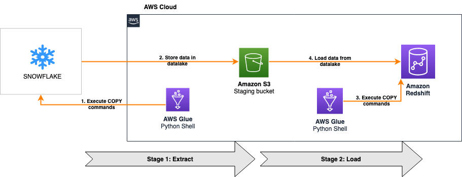
You can also automate the preceding COPY commands using tasks, which can be scheduled to run at a set frequency for automatic copy of CDC data from Snowflake to Amazon S3.
  10. Use the ACCOUNTADMIN role to assign the EXECUTE TASK privilege. In this scenario, we’re assigning the privileges to the SYSADMIN role:
    USE ROLE accountadmin;
    GRANT EXECUTE TASK, EXECUTE MANAGED TASK ON ACCOUNT TO ROLE sysadmin;

  11. Use the SYSADMIN role to create three separate tasks to run three COPY commands every 5 minutes: USE ROLE sysadmin;
    /* Task to offload Customer CDC table */ 
    CREATE TASK sf_rs_customer_cdc 
    WAREHOUSE = SMALL 
    SCHEDULE = 'USING CRON 5 * * * * UTC' 
    AS 
    COPY INTO @unload_to_s3/customer_stg/ 
    FROM (select *, sysdate() as LAST_UPDATED_TS from demo_db.blog_demo.customer_check) 
    FILE_FORMAT = (TYPE = PARQUET) 
    OVERWRITE = TRUE 
    HEADER = TRUE;
    /*Task to offload Orders CDC table */ 
    CREATE TASK sf_rs_orders_cdc 
    WAREHOUSE = SMALL 
    SCHEDULE = 'USING CRON 5 * * * * UTC' 
    AS 
    COPY INTO @unload_to_s3/orders_stg/ 
    FROM (select *, sysdate() as LAST_UPDATED_TS from demo_db.blog_demo.orders_check)
    FILE_FORMAT = (TYPE = PARQUET)
    OVERWRITE = TRUE HEADER = TRUE;

    /* Task to offload Lineitem CDC table */ 
    CREATE TASK sf_rs_lineitem_cdc 
    WAREHOUSE = SMALL 
    SCHEDULE = 'USING CRON 5 * * * * UTC' 
    AS 
    COPY INTO @unload_to_s3/lineitem_stg/ 
    FROM (select *, sysdate() as LAST_UPDATED_TS from demo_db.blog_demo.lineitem_check)
    FILE_FORMAT = (TYPE = PARQUET)
    OVERWRITE = TRUE HEADER = TRUE;

    When the tasks are first created, they’re in a SUSPENDED state.

  12. Alter the three tasks and set them to RESUME state:
    ALTER TASK sf_rs_customer_cdc RESUME;
    ALTER TASK sf_rs_orders_cdc RESUME;
    ALTER TASK sf_rs_lineitem_cdc RESUME;

  13. Validate that all three tasks have been resumed successfully: SHOW TASKS;unload-setp-13-valNow the tasks will run every 5 minutes and look for new data in the stream tables to offload to Amazon S3.As soon as data is migrated from Snowflake to Amazon S3, Redshift Auto Loader automatically infers the schema and instantly creates corresponding tables in Amazon Redshift. Then, by default, it starts loading data from Amazon S3 to Amazon Redshift every 5 minutes. You can also change the default setting of 5 minutes.
  14. On the Amazon Redshift console, launch the query editor v2 and connect to your Amazon Redshift cluster.
  15. Browse to the dev database, public schema, and expand Tables.
    You can see three staging tables created with the same name as the corresponding folders in Amazon S3.
  16. Validate the data in one of the tables by running the following query:SELECT * FROM "dev"."public"."customer_stg";unload-step-16-val

Configure the Redshift Auto Loader utility

The Redshift Auto Loader makes data ingestion to Amazon Redshift significantly easier because it automatically loads data files from Amazon S3 to Amazon Redshift. The files are mapped to the respective tables by simply dropping files into preconfigured locations on Amazon S3. For more details about the architecture and internal workflow, refer to the GitHub repo.

We use an AWS CloudFormation template to set up Redshift Auto Loader. Complete the following steps:

  1. Launch the CloudFormation template.
  2. Choose Next.
    autoloader-step-2
  3. For Stack name, enter a name.
  4. Provide the parameters listed in the following table.

    CloudFormation Template Parameter Allowed Values Description
    RedshiftClusterIdentifier Amazon Redshift cluster identifier Enter the Amazon Redshift cluster identifier.
    DatabaseUserName Database user name in the Amazon Redshift cluster The Amazon Redshift database user name that has access to run the SQL script.
    DatabaseName S3 bucket name The name of the Amazon Redshift primary database where the SQL script is run.
    DatabaseSchemaName Database name in Amazon Redshift The Amazon Redshift schema name where the tables are created.
    RedshiftIAMRoleARN Default or the valid IAM role ARN attached to the Amazon Redshift cluster The IAM role ARN associated with the Amazon Redshift cluster. Your default IAM role is set for the cluster and has access to your S3 bucket, leave it at the default.
    CopyCommandOptions Copy option; default is delimiter ‘|’ gzip

    Provide the additional COPY command data format parameters.

    If InitiateSchemaDetection = Yes, then the process attempts to detect the schema and automatically set the suitable copy command options.

    In the event of failure on schema detection or when InitiateSchemaDetection = No, then this value is used as the default COPY command options to load data.

    SourceS3Bucket S3 bucket name The S3 bucket where the data is stored. Make sure the IAM role that is associated to the Amazon Redshift cluster has access to this bucket.
    InitiateSchemaDetection Yes/No

    Set to Yes to dynamically detect the schema prior to file load and create a table in Amazon Redshift if it doesn’t exist already. If a table already exists, then it won’t drop or recreate the table in Amazon Redshift.

    If schema detection fails, the process uses the default COPY options as specified in CopyCommandOptions.

    The Redshift Auto Loader uses the COPY command to load data into Amazon Redshift. For this post, set CopyCommandOptions as follows, and configure any supported COPY command options:

    delimiter '|' dateformat 'auto' TIMEFORMAT 'auto'

    autoloader-input-parameters

  5. Choose Next.
  6. Accept the default values on the next page and choose Next.
  7. Select the acknowledgement check box and choose Create stack.
    autoloader-step-7
  8. Monitor the progress of the Stack creation and wait until it is complete.
  9. To verify the Redshift Auto Loader configuration, sign in to the Amazon S3 console and navigate to the S3 bucket you provided.
    You should see a new directory s3-redshift-loader-source is created.
    autoloader-step-9

Copy all the data files exported from Snowflake under s3-redshift-loader-source.

Merge the data from the CDC S3 staging tables to Amazon Redshift tables

To merge your data from Amazon S3 to Amazon Redshift, complete the following steps:

  1. Create a temporary staging table merge_stg and insert all the rows from the S3 staging table that have metadata_action as INSERT, using the following code. This includes all the new inserts as well as the update.
    CREATE TEMP TABLE merge_stg 
    AS
    SELECT * FROM
    (
    SELECT *, DENSE_RANK() OVER (PARTITION BY c_custkey ORDER BY last_updated_ts DESC
    ) AS rnk
    FROM customer_stg WHERE rnk = 1 AND metadata$action = 'INSERT'

    The preceding code uses a window function DENSE_RANK() to select the latest entries for a given c_custkey by assigning a rank to each row for a given c_custkey and arrange the data in descending order using last_updated_ts. We then select the rows with rnk=1 and metadata$action = ‘INSERT’ to capture all the inserts.

  2. Use the S3 staging table customer_stg to delete the records from the base table customer, which are marked as deletes or updates:
    DELETE FROM customer 
    USING customer_stg 
    WHERE customer.c_custkey = customer_stg.c_custkey;

    This deletes all the rows that are present in the CDC S3 staging table, which takes care of rows marked for deletion and updates.

  3. Use the temporary staging table merge_stg to insert the records marked for updates or inserts:
    INSERT INTO customer 
    SELECT c_custkey, c_name, c_address, c_nationkey, c_phone, c_acctbal, c_mktsegment, c_comment 
    FROM merge_stg;

  4. Truncate the staging table, because we have already updated the target table:truncate customer_stg;
  5. You can also run the preceding steps as a stored procedure:
    CREATE OR REPLACE PROCEDURE merge_customer()
    AS $$
    BEGIN
    /*CREATING TEMP TABLE TO GET THE MOST LATEST RECORDS FOR UPDATES/NEW INSERTS*/
    CREATE TEMP TABLE merge_stg AS
    SELECT * FROM
    (
    SELECT *, DENSE_RANK() OVER (PARTITION BY c_custkey ORDER BY last_updated_ts DESC ) AS rnk
    FROM customer_stg
    )
    WHERE rnk = 1 AND metadata$action = 'INSERT';
    /* DELETING FROM THE BASE TABLE USING THE CDC STAGING TABLE ALL THE RECORDS MARKED AS DELETES OR UPDATES*/
    DELETE FROM customer
    USING customer_stg
    WHERE customer.c_custkey = customer_stg.c_custkey;
    /*INSERTING NEW/UPDATED RECORDS IN THE BASE TABLE*/ 
    INSERT INTO customer
    SELECT c_custkey, c_name, c_address, c_nationkey, c_phone, c_acctbal, c_mktsegment, c_comment
    FROM merge_stg;
    truncate customer_stg;
    END;
    $$ LANGUAGE plpgsql;

    For example, let’s look at the before and after states of the customer table when there’s been a change in data for a particular customer.

    The following screenshot shows the new changes recorded in the customer_stg table for c_custkey = 74360.
    merge-process-new-changes
    We can see two records for a customer with c_custkey=74360 one with metadata$action as DELETE and one with metadata$action as INSERT. That means the record with c_custkey was updated at the source and these changes need to be applied to the target customer table in Amazon Redshift.

    The following screenshot shows the current state of the customer table before these changes have been merged using the preceding stored procedure:
    merge-process-current-state

  6. Now, to update the target table, we can run the stored procedure as follows: CALL merge_customer()The following screenshot shows the final state of the target table after the stored procedure is complete.
    merge-process-after-sp

Run the stored procedure on a schedule

You can also run the stored procedure on a schedule via Amazon EventBridge. The scheduling steps are as follows:

  1. On the EventBridge console, choose Create rule.
    sp-schedule-1
  2. For Name, enter a meaningful name, for example, Trigger-Snowflake-Redshift-CDC-Merge.
  3. For Event bus, choose default.
  4. For Rule Type, select Schedule.
  5. Choose Next.
    sp-schedule-step-5
  6. For Schedule pattern, select A schedule that runs at a regular rate, such as every 10 minutes.
  7. For Rate expression, enter Value as 5 and choose Unit as Minutes.
  8. Choose Next.
    sp-schedule-step-8
  9. For Target types, choose AWS service.
  10. For Select a Target, choose Redshift cluster.
  11. For Cluster, choose the Amazon Redshift cluster identifier.
  12. For Database name, choose dev.
  13. For Database user, enter a user name with access to run the stored procedure. It uses temporary credentials to authenticate.
  14. Optionally, you can also use AWS Secrets Manager for authentication.
  15. For SQL statement, enter CALL merge_customer().
  16. For Execution role, select Create a new role for this specific resource.
  17. Choose Next.
    sp-schedule-step-17
  18. Review the rule parameters and choose Create rule.

After the rule has been created, it automatically triggers the stored procedure in Amazon Redshift every 5 minutes to merge the CDC data into the target table.

Configure Amazon Redshift to share the identified data with AWS Data Exchange

Now that you have the data stored inside Amazon Redshift, you can publish it to customers using AWS Data Exchange.

  1. In Amazon Redshift, using any query editor, create the data share and add the tables to be shared:
    CREATE DATASHARE salesshare MANAGEDBY ADX;
    ALTER DATASHARE salesshare ADD SCHEMA tpch_sf1;
    ALTER DATASHARE salesshare ADD TABLE tpch_sf1.customer;

    ADX-step1

  2. On the AWS Data Exchange console, create your dataset.
  3. Select Amazon Redshift datashare.
    ADX-step3-create-datashare
  4. Create a revision in the dataset.
    ADX-step4-create-revision
  5. Add assets to the revision (in this case, the Amazon Redshift data share).
    ADX-addassets
  6. Finalize the revision.
    ADX-step-6-finalizerevision

After you create the dataset, you can publish it to the public catalog or directly to customers as a private product. For instructions on how to create and publish products, refer to NEW – AWS Data Exchange for Amazon Redshift

Clean up

To avoid incurring future charges, complete the following steps:

  1. Delete the CloudFormation stack used to create the Redshift Auto Loader.
  2. Delete the Amazon Redshift cluster created for this demonstration.
  3. If you were using an existing cluster, drop the created external table and external schema.
  4. Delete the S3 bucket you created.
  5. Delete the Snowflake objects you created.

Conclusion

In this post, we demonstrated how you can set up a fully integrated process that continuously replicates data from Snowflake to Amazon Redshift and then uses Amazon Redshift to offer data to downstream clients over AWS Data Exchange. You can use the same architecture for other purposes, such as sharing data with other Amazon Redshift clusters within the same account, cross-accounts, or even cross-Regions if needed.


About the Authors

Raks KhareRaks Khare is an Analytics Specialist Solutions Architect at AWS based out of Pennsylvania. He helps customers architect data analytics solutions at scale on the AWS platform.

Ekta Ahuja is a Senior Analytics Specialist Solutions Architect at AWS. She is passionate about helping customers build scalable and robust data and analytics solutions. Before AWS, she worked in several different data engineering and analytics roles. Outside of work, she enjoys baking, traveling, and board games.

Tahir Aziz is an Analytics Solution Architect at AWS. He has worked with building data warehouses and big data solutions for over 13 years. He loves to help customers design end-to-end analytics solutions on AWS. Outside of work, he enjoys traveling
and cooking.

Ahmed Shehata is a Senior Analytics Specialist Solutions Architect at AWS based on Toronto. He has more than two decades of experience helping customers modernize their data platforms, Ahmed is passionate about helping customers build efficient, performant and scalable Analytic solutions.

Migrate from Snowflake to Amazon Redshift using AWS Glue Python shell

Post Syndicated from Raks Khare original https://aws.amazon.com/blogs/big-data/migrate-from-snowflake-to-amazon-redshift-using-aws-glue-python-shell/

As the most widely used cloud data warehouse, Amazon Redshift makes it simple and cost-effective to analyze your data using standard SQL and your existing ETL (extract, transform, and load), business intelligence (BI), and reporting tools. Tens of thousands of customers use Amazon Redshift to analyze exabytes of data per day and power analytics workloads such as BI, predictive analytics, and real-time streaming analytics without having to manage the data warehouse infrastructure. It natively integrates with other AWS services, facilitating the process of building enterprise-grade analytics applications in a manner that is not only cost-effective, but also avoids point solutions.

We are continuously innovating and releasing new features of Amazon Redshift, enabling the implementation of a wide range of data use cases and meeting requirements with performance and scale. For example, Amazon Redshift Serverless allows you to run and scale analytics workloads without having to provision and manage data warehouse clusters. Other features that help power analytics at scale with Amazon Redshift include automatic concurrency scaling for read and write queries, automatic workload management (WLM) for concurrency scaling, automatic table optimization, the new RA3 instances with managed storage to scale cloud data warehouses and reduce costs, cross-Region data sharing, data exchange, and the SUPER data type to store semi-structured data or documents as values. For the latest feature releases for Amazon Redshift, see Amazon Redshift What’s New. In addition to improving performance and scale, you can also gain up to three times better price performance with Amazon Redshift than other cloud data warehouses.

To take advantage of the performance, security, and scale of Amazon Redshift, customers are looking to migrate their data from their existing cloud warehouse in a way that is both cost optimized and performant. This post describes how to migrate a large volume of data from Snowflake to Amazon Redshift using AWS Glue Python shell in a manner that meets both these goals.

AWS Glue is serverless data integration service that makes it easy to discover, prepare, and combine data for analytics, machine learning (ML), and application development. AWS Glue provides all the capabilities needed for data integration, allowing you to analyze your data in minutes instead of weeks or months. AWS Glue supports the ability to use a Python shell job to run Python scripts as a shell, enabling you to author ETL processes in a familiar language. In addition, AWS Glue allows you to manage ETL jobs using AWS Glue workflows, Amazon Managed Workflows for Apache Airflow (Amazon MWAA), and AWS Step Functions, automating and facilitating the orchestration of ETL steps.

Solution overview

The following architecture shows how an AWS Glue Python shell job migrates the data from Snowflake to Amazon Redshift in this solution.

Architecture

The solution is comprised of two stages:

  • Extract – The first part of the solution extracts data from Snowflake into an Amazon Simple Storage Service (Amazon S3) data lake
  • Load – The second part of the solution reads the data from the same S3 bucket and loads it into Amazon Redshift

For both stages, we connect the AWS Glue Python shell jobs to Snowflake and Amazon Redshift using database connectors for Python. The first AWS Glue Python shell job reads a SQL file from an S3 bucket to run the relevant COPY commands on the Snowflake database using Snowflake compute capacity and parallelism to migrate the data to Amazon S3. When this is complete, the second AWS Glue Python shell job reads another SQL file, and runs the corresponding COPY commands on the Amazon Redshift database using Redshift compute capacity and parallelism to load the data from the same S3 bucket.

Both jobs are orchestrated using AWS Glue workflows, as shown in the following screenshot. The workflow pushes data processing logic down to the respective data warehouses by running COPY commands on the databases themselves, minimizing the processing capacity required by AWS Glue to just the resources needed to run the Python scripts. The COPY commands load data in parallel both to and from Amazon S3, providing one of the fastest and most scalable mechanisms to transfer data from Snowflake to Amazon Redshift.

Because all heavy lifting around data processing is pushed down to the data warehouses, this solution is designed to provide a cost-optimized and highly performant mechanism to migrate a large volume of data from Snowflake to Amazon Redshift with ease.

Glue Workflow

The entire solution is packaged in an AWS CloudFormation template for simplicity of deployment and automatic provisioning of most of the required resources and permissions.

The high-level steps to implement the solution are as follows:

  1. Generate the Snowflake SQL file.
  2. Deploy the CloudFormation template to provision the required resources and permissions.
  3. Provide Snowflake access to newly created S3 bucket.
  4. Run the AWS Glue workflow to migrate the data.

Prerequisites

Before you get started, you can optionally build the latest version of the Snowflake Connector for Python package locally and generate the wheel (.whl) package. For instructions, refer to How to build.

If you don’t provide the latest version of the package, the CloudFormation template uses a pre-built .whl file that may not be on the most current version of Snowflake Connector for Python.

By default, the CloudFormation template migrates data from all tables in the TPCH_SF1 schema of the SNOWFLAKE_SAMPLE_DATA database, which is a sample dataset provided by Snowflake when an account is created. The following stored procedure is used to dynamically generate the Snowflake COPY commands required to migrate the dataset to Amazon S3. It accepts the database name, schema name, and stage name as the parameters.

CREATE OR REPLACE PROCEDURE generate_copy(db_name VARCHAR, schema_name VARCHAR, stage_name VARCHAR)
   returns varchar not null
   language javascript
   as
   $$
var return_value = "";
var sql_query = "select table_catalog, table_schema, lower(table_name) as table_name from " + DB_NAME + ".information_schema.tables where table_schema = '" + SCHEMA_NAME + "'" ;
   var sql_statement = snowflake.createStatement(
          {
          sqlText: sql_query
          }
       );
/* Creates result set */
var result_scan = sql_statement.execute();
while (result_scan.next())  {
       return_value += "\n";
       return_value += "COPY INTO @"
       return_value += STAGE_NAME
       return_value += "/"
       return_value += result_scan.getColumnValue(3);
       return_value += "/"
       return_value += "\n";
       return_value += "FROM ";
       return_value += result_scan.getColumnValue(1);
       return_value += "." + result_scan.getColumnValue(2);
       return_value += "." + result_scan.getColumnValue(3);
       return_value += "\n";
       return_value += "FILE_FORMAT = (TYPE = CSV FIELD_DELIMITER = '|' COMPRESSION = GZIP)";
       return_value += "\n";
       return_value += "OVERWRITE = TRUE;"
       return_value += "\n";
       }
return return_value;
$$
;

Deploy the required resources and permissions using AWS CloudFormation

You can use the provided CloudFormation template to deploy this solution. This template automatically provisions an Amazon Redshift cluster with your desired configuration in a private subnet, maintaining a high standard of security.

  1. Sign in to the AWS Management Console, preferably as admin user.
  2. Select your desired Region, preferably the same Region where your Snowflake instance is provisioned.
  3. Choose Launch Stack:
  4. Choose Next.
  5. For Stack name, enter a meaningful name for the stack, for example, blog-resources.

The Parameters section is divided into two subsections: Source Snowflake Infrastructure and Target Redshift Configuration.

  1. For Snowflake Unload SQL Script, it defaults to S3 location (URI) of a SQL file which migrates the sample data in the TPCH_SF1 schema of the SNOWFLAKE_SAMPLE_DATA database.
  2. For Data S3 Bucket, enter a prefix for the name of the S3 bucket that is automatically provisioned to stage the Snowflake data, for example, sf-migrated-data.
  3. For Snowflake Driver, if applicable, enter the S3 location (URI) of the .whl package built earlier as a prerequisite. By default, it uses a pre-built .whl file.
  4. For Snowflake Account Name, enter your Snowflake account name.

You can use the following query in Snowflake to return your Snowflake account name:

SELECT CURRENT_ACCOUNT();
  1. For Snowflake Username, enter your user name to connect to the Snowflake account.
  2. For Snowflake Password, enter the password for the preceding user.
  3. For Snowflake Warehouse Name, enter the warehouse name for running the SQL queries.

Make sure the aforementioned user has access to the warehouse.

  1. For Snowflake Database Name, enter the database name. The default is SNOWFLAKE_SAMPLE_DATA.
  2. For Snowflake Schema Name, enter schema name. The default is TPCH_SF1.

CFN Param Snowflake

  1. For VPC CIDR Block, enter the desired CIDR block of Redshift cluster. The default is 10.0.0.0/16.
  2. For Subnet 1 CIDR Block, enter the CIDR block of the first subnet. The default is 10.0.0.0/24.
  3. For Subnet 2 CIDR Block, enter the CIDR block of the first subnet. The default is 10.0.1.0/24.
  4. For Redshift Load SQL Script, it defaults to S3 location (URI) of a SQL file which migrates the sample data in S3 to Redshift.

The following database view in Redshift is used to dynamically generate Redshift COPY commands required to migrate the dataset from Amazon S3. It accepts the schema name as the filter criteria.

CREATE OR REPLACE VIEW v_generate_copy
AS
SELECT
    schemaname ,
    tablename  ,
    seq        ,
    ddl
FROM
    (
        SELECT
            table_id   ,
            schemaname ,
            tablename  ,
            seq        ,
            ddl
        FROM
            (
                --COPY TABLE
                SELECT
                    c.oid::bigint  as table_id   ,
                    n.nspname      AS schemaname ,
                    c.relname      AS tablename  ,
                    0              AS seq        ,
                    'COPY ' + n.nspname + '.' + c.relname + ' FROM ' AS ddl
                FROM
                    pg_namespace AS n
                INNER JOIN
                    pg_class AS c
                ON
                    n.oid = c.relnamespace
                WHERE
                    c.relkind = 'r'
                --COPY TABLE continued                
                UNION                
                SELECT
                    c.oid::bigint as table_id   ,
                    n.nspname     AS schemaname ,
                    c.relname     AS tablename  ,
                    2             AS seq        ,
                    '''${' + '2}' + c.relname + '/'' iam_role ''${' + '1}'' gzip delimiter ''|'' EMPTYASNULL REGION ''us-east-1''' AS ddl
                FROM
                    pg_namespace AS n
                INNER JOIN
                    pg_class AS c
                ON
                    n.oid = c.relnamespace
                WHERE
                    c.relkind = 'r'
                --END SEMICOLON                
                UNION                
                SELECT
                    c.oid::bigint as table_id  ,
                    n.nspname     AS schemaname,
                    c.relname     AS tablename ,
                    600000005     AS seq       ,
                    ';'           AS ddl
                FROM
                    pg_namespace AS n
                INNER JOIN
                    pg_class AS c
                ON
                    n.oid = c.relnamespace
                WHERE
                    c.relkind = 'r' 
             )
        ORDER BY
            table_id  ,
            schemaname,
            tablename ,
            seq 
    );

SELECT ddl
FROM v_generate_copy
WHERE schemaname = 'tpch_sf1';
  1. For Redshift Database Name, enter your desired database name, for example, dev.
  2. For Number of Redshift Nodes, enter the desired compute nodes, for example, 2.
  3. For Redshift Node Type, choose the desired node type, for example, ra3.4xlarge.
  4. For Redshift Password, enter your desired password with the following constraints: it must be 8–64 characters in length, and contain at least one uppercase letter, one lowercase letter, and one number.
  5. For Redshift Port, enter the Amazon Redshift port number to connect to. The default port is 5439.

CFN Param Redshift 1 CFN Param Redshift 2

  1. Choose Next.
  2. Review and choose Create stack.

It takes around 5 minutes for the template to finish creating all resources and permissions. Most of the resources have the prefix of the stack name you specified for easy identification of the resources later. For more details on the deployed resources, see the appendix at the end of this post.

Create an IAM role and external Amazon S3 stage for Snowflake access to the data S3 bucket

In order for Snowflake to access the TargetDataS3Bucket created earlier by CloudFormation template, you must create an AWS Identity and Access Management (IAM) role and external Amazon S3 stage for Snowflake access to the S3 bucket. For instructions, refer to Configuring Secure Access to Amazon S3.

When you create an external stage in Snowflake, use the value for TargetDataS3Bucket on the Outputs tab of your deployed CloudFormation stack for the Amazon S3 URL of your stage.

CF Output

Make sure to name the external stage unload_to_s3 if you’re migrating the sample data using the default scripts provided in the CloudFormation template.

Convert Snowflake tables to Amazon Redshift

You can simply run the following DDL statements to create TPCH_SF1 schema objects in Amazon Redshift. You can also use AWS Schema Conversion Tool (AWS SCT) to convert Snowflake custom objects to Amazon Redshift. For instructions on converting your schema, refer to Accelerate Snowflake to Amazon Redshift migration using AWS Schema Conversion Tool.

CREATE SCHEMA TPCH_SF1;
SET SEARCH_PATH to TPCH_SF1;
CREATE TABLE customer (
  c_custkey int8 not null ,
  c_name varchar(25) not null,
  c_address varchar(40) not null,
  c_nationkey int4 not null,
  c_phone char(15) not null,
  c_acctbal numeric(12,2) not null,
  c_mktsegment char(10) not null,
  c_comment varchar(117) not null,
  Primary Key(C_CUSTKEY)
) ;

CREATE TABLE lineitem (
  l_orderkey int8 not null ,
  l_partkey int8 not null,
  l_suppkey int4 not null,
  l_linenumber int4 not null,
  l_quantity numeric(12,2) not null,
  l_extendedprice numeric(12,2) not null,
  l_discount numeric(12,2) not null,
  l_tax numeric(12,2) not null,
  l_returnflag char(1) not null,
  l_linestatus char(1) not null,
  l_shipdate date not null ,
  l_commitdate date not null,
  l_receiptdate date not null,
  l_shipinstruct char(25) not null,
  l_shipmode char(10) not null,
  l_comment varchar(44) not null,
  Primary Key(L_ORDERKEY, L_LINENUMBER)
)  ;

CREATE TABLE nation (
  n_nationkey int4 not null,
  n_name char(25) not null ,
  n_regionkey int4 not null,
  n_comment varchar(152) not null,
  Primary Key(N_NATIONKEY)                                
) ;

CREATE TABLE orders (
  o_orderkey int8 not null,
  o_custkey int8 not null,
  o_orderstatus char(1) not null,
  o_totalprice numeric(12,2) not null,
  o_orderdate date not null,
  o_orderpriority char(15) not null,
  o_clerk char(15) not null,
  o_shippriority int4 not null,
  o_comment varchar(79) not null,
  Primary Key(O_ORDERKEY)
) ;

CREATE TABLE part (
  p_partkey int8 not null ,
  p_name varchar(55) not null,
  p_mfgr char(25) not null,
  p_brand char(10) not null,
  p_type varchar(25) not null,
  p_size int4 not null,
  p_container char(10) not null,
  p_retailprice numeric(12,2) not null,
  p_comment varchar(23) not null,
  PRIMARY KEY (P_PARTKEY)
) ;

CREATE TABLE partsupp (
  ps_partkey int8 not null,
  ps_suppkey int4 not null,
  ps_availqty int4 not null,
  ps_supplycost numeric(12,2) not null,
  ps_comment varchar(199) not null,
  Primary Key(PS_PARTKEY, PS_SUPPKEY)
) ;

CREATE TABLE region (
  r_regionkey int4 not null,
  r_name char(25) not null ,
  r_comment varchar(152) not null,
  Primary Key(R_REGIONKEY)                             
) ;

CREATE TABLE supplier (
  s_suppkey int4 not null,
  s_name char(25) not null,
  s_address varchar(40) not null,
  s_nationkey int4 not null,
  s_phone char(15) not null,
  s_acctbal numeric(12,2) not null,
  s_comment varchar(101) not null,
  Primary Key(S_SUPPKEY)
);

Run an AWS Glue workflow for data migration

When you’re ready to start the data migration, complete the following steps:

  1. On the AWS Glue console, choose Workflows in the navigation pane.
  2. Select the workflow to run (<stack name>snowflake-to-redshift-migration).
  3. On the Actions menu, choose Run.Glue Workflow Run
  4. To check the status of the workflow, choose the workflow and on the History tab, select the Run ID and choose View run details.
    Glue Workflow Status
  5. When the workflow is complete, navigate to the Amazon Redshift console and launch the Amazon Redshift query editor v2 to verify the successful migration of data.
  6. Run the following query in Amazon Redshift to get row counts of all tables migrated from Snowflake to Amazon Redshift. Make sure to adjust the table_schema value accordingly if you’re not migrating the sample data.
SELECT tab.table_schema,
       tab.table_name,
       nvl(tinf.tbl_rows,0) tbl_rows,
       nvl(tinf.size,0) size
FROM svv_tables tab
LEFT JOIN svv_table_info tinf 
          on tab.table_schema = tinf.schema 
          and tab.table_name = tinf.”table”
WHERE tab.table_type = 'BASE TABLE'
      and tab.table_schema in ('tpch_sf1')
ORDER BY tbl_rows;

Redshift Editor

  1. Run the following query in Snowflake to compare and validate the data:
USE DATABASE snowflake_sample_data;
SELECT  TABLE_CATALOG,
        TABLE_SCHEMA,
        TABLE_NAME,
        ROW_COUNT,
        BYTES AS SIZE,
        COMMENT
FROM INFORMATION_SCHEMA.TABLES
WHERE TABLE_SCHEMA = 'TPCH_SF1'
ORDER BY ROW_COUNT;

Snowflake Editor

Clean up

To avoid incurring future charges, delete the resources you created as part of the CloudFormation stack by navigating to the AWS CloudFormation console, selecting the stack blog-resources, and choosing Delete.

Conclusion

In this post, we discussed how to perform an efficient, fast, and cost-effective migration from Snowflake to Amazon Redshift. Migrations from one data warehouse environment to another can typically be very time-consuming and resource-intensive; this solution uses the power of cloud-based compute by pushing down the processing to the respective warehouses. Orchestrating this migration with the AWS Glue Python shell provides additional cost optimization.

With this solution, you can facilitate your migration from Snowflake to Amazon Redshift. If you’re interested in further exploring the potential of using Amazon Redshift, please reach out to your AWS Account Team for a proof of concept.

Appendix: Resources deployed by AWS CloudFormation

The CloudFormation stack deploys the following resources in your AWS account:

  • Networking resourcesAmazon Virtual Private Cloud (Amazon VPC), subnets, ACL, and security group.
  • Amazon S3 bucket – This is referenced as TargetDataS3Bucket on the Outputs tab of the CloudFormation stack. This bucket holds the data being migrated from Snowflake to Amazon Redshift.
  • AWS Secrets Manager secrets – Two secrets in AWS Secrets Manager store credentials for Snowflake and Amazon Redshift.
  • VPC endpoints – The two VPC endpoints are deployed to establish a private connection from VPC resources like AWS Glue to services that run outside of the VPC, such as Secrets Manager and Amazon S3.
  • IAM roles – IAM roles for AWS Glue, Lambda, and Amazon Redshift. If the CloudFormation template is to be deployed in a production environment, you need to adjust the IAM policies so they’re not as permissive as presented in this post (which were set for simplicity and demonstration). Particularly, AWS Glue and Amazon Redshift don’t require all the actions granted in the *FullAccess policies, which would be considered overly permissive.
  • Amazon Redshift cluster – An Amazon Redshift cluster is created in a private subnet, which isn’t publicly accessible.
  • AWS Glue connection – The connection for Amazon Redshift makes sure that the AWS Glue job runs within the same VPC as Amazon Redshift. This also ensures that AWS Glue can access the Amazon Redshift cluster in a private subnet.
  • AWS Glue jobs – Two AWS Glue Python shell jobs are created:
    • <stack name>-glue-snowflake-unload – The first job runs the SQL scripts in Snowflake to copy data from the source database to Amazon S3. The Python script is available in S3. The Snowflake job accepts two parameters:
      • SQLSCRIPT – The Amazon S3 location of the SQL script to run in Snowflake to migrate data to Amazon S3. This is referenced as the Snowflake Unload SQL Script parameter in the input section of the CloudFormation template.
      • SECRET – The Secrets Manager ARN that stores Snowflake connection details.
    • <stack name>-glue-redshift-load – The second job runs another SQL script in Amazon Redshift to copy data from Amazon S3 to the target Amazon Redshift database. The Python script link is available in S3. The Amazon Redshift job accepts three parameters:
      • SQLSCRIPT – The Amazon S3 location of the SQL script to run in Amazon Redshift to migrate data from Amazon S3. If you provide custom SQL script to migrate the Snowflake data to Amazon S3 (as mentioned in the prerequisites), the file location is referenced as LoadFileLocation on the Outputs tab of the CloudFormation stack.
      • SECRET – The Secrets Manager ARN that stores Amazon Redshift connection details.
      • PARAMS – This includes any additional parameters required for the SQL script, including the Amazon Redshift IAM role used in the COPY commands and the S3 bucket staging the Snowflake data. Multiple parameter values can be provided separated by a comma.
  • AWS Glue workflow – The orchestration of Snowflake and Amazon Redshift AWS Glue Python shell jobs is managed via an AWS Glue workflow. The workflow <stack name>snowflake-to-redshift-migration runs later for actual migration of data.

About the Authors

Raks KhareRaks Khare is an Analytics Specialist Solutions Architect at AWS based out of Pennsylvania. He helps customers architect data analytics solutions at scale on the AWS platform.

Julia BeckJulia Beck is an Analytics Specialist Solutions Architect at AWS. She supports customers in validating analytics solutions by architecting proof of concept workloads designed to meet their specific needs.