When migrating from Teradata BTEQ (Basic Teradata Query) to Amazon Redshift RSQL, following established best practices helps ensure maintainable, efficient, and reliable code. While the AWS Schema Conversion Tool (AWS SCT) automatically handles the basic conversion of BTEQ scripts to RSQL, it primarily focuses on SQL syntax translation and basic script conversion. However, to achieve optimal performance, better maintainability, and full compatibility with the architecture of Amazon Redshift, additional optimization and standardization are needed.
The best practices that we share in this post complement the automated conversion supplied by AWS SCT by addressing areas such as performance tuning, error handling improvements, script modularity, logging enhancements, and Amazon Redshift-specific optimizations that AWS SCT might not fully implement. These practices can help you transform automatically converted code into production-ready, efficient RSQL scripts that fully use the capabilities of Amazon Redshift.
BTEQ
BTEQ is Teradata’s legacy command-line SQL tool that has served as the primary interface for Teradata databases since the 1980s. It’s a powerful utility that combines SQL querying capabilities with scripting features; you can use it to perform various tasks from data extraction and reporting to complex database administration. BTEQ’s robustness lies in its ability to handle direct database interactions, manage sessions, process variables, and execute conditional logic while providing comprehensive error handling and report formatting capabilities.
RSQL is a modern command-line client tool provided by Amazon Redshift and is specifically designed to execute SQL commands and scripts in the AWS ecosystem. Similar to PostgreSQL’s psql but optimized for the unique architecture of Amazon Redshift, RSQL offers seamless SQL query execution, efficient script processing, and sophisticated result set handling. It stands out for its native integration with AWS services, making it a powerful tool for modern data warehousing operations.
The transition from BTEQ to RSQL has become increasingly relevant as organizations embrace cloud transformation. This migration is driven by several compelling factors. Businesses are moving from on-premises Teradata systems to Amazon Redshift to take advantage of cloud benefits. Cost optimization plays a crucial role in these moves, because Amazon Redshift typically offers more economical data warehousing solutions with its pay-as-you-go pricing model.
Furthermore, organizations want to modernize their data architecture to take advantage of enhanced security features, better scalability, and seamless integration with other AWS services. The migration also brings performance benefits through columnar storage, parallel processing capabilities, and optimized query performance offered by Amazon Redshift, making it an attractive destination for enterprises looking to modernize their data infrastructure.
Best practices for BTEQ to RSQL migration
Let’s explore key practices across code structure, performance optimization, error handling, and Redshift-specific considerations that will help you create robust and efficient RSQL scripts.
Parameter files
Parameters in RSQL function as variables that store and pass values to your scripts, similar to BTEQ’s .SET VARIABLE functionality. Instead of hardcoding schema names, table names, or configuration values directly in RSQL scripts, use dynamic parameters that can be modified for different environments (dev, test, prod). This approach reduces manual errors, simplifies maintenance, and supports better version control by keeping sensitive values separate from code.
Create a separate shell script containing environment variables:
Debugging and troubleshooting SQL scripts can be challenging, especially when dealing with complex queries or error scenarios. To simplify this process, it’s recommended to enable query logging in RSQL scripts.
RSQL provides the echo-queries option, which prints the executed SQL queries along with their execution status. By invoking the RSQL client with this option, you can track the progress of your script and identify potential issues.
rsql --echo-queries -D testiam
Here testiam represents a DSN connection configured in odbc.ini with an IAM profile.
You can store these logs by redirecting the output when executing your RSQL script:
```
sh <path to RSQL file>/<RSQL file name>.sh  >  <log file name>.log
```
With query logging is enabled, you can examine the output and identify the specific query that caused an error or unexpected behavior. This information can be invaluable when troubleshooting and optimizing your RSQL scripts.
Error handling with incremental exit codes
Implement robust error handling using incremental exit codes to identify specific failure points. Proper error handling is crucial in a scripting environment, and RSQL is no exception. In BTEQ scripts, errors were typically handled by checking the error code and taking appropriate actions. However, in RSQL, the approach is slightly different. To help ensure robust error handling and straightforward troubleshooting, it’s recommended that you implement incremental exit codes at the end of each SQL operation.The incremental exit code approach works as follows:
After executing a SQL statement (such as SELECT, INSERT, UPDATE, and so on.), check the value of the :ERROR variable.
If the :ERROR variable is non-zero, it indicates that an error occurred during the execution of the SQL statement.
Print the error message, error code, and additional relevant information using RSQL commands such as \echo, \remark, and so on.
Exit the script with an appropriate exit code using the \exit command, where the exit code represents the specific operation that failed.
By using incremental exit codes, you can identify the point of failure within the script. This approach not only aids in troubleshooting but also allows for better integration with continuous integration and deployment (CI/CD) pipelines, where specific exit codes can trigger appropriate actions.
Example:
SELECT * FROM $STAGING_TABLE_SCHEMA.SAMPLE_TABLE;
\if :ERROR <> 0
      \echo 'Error occurred in executing the select operation on table $STAGING_TABLE_SCHEMA.SAMPLE_TABLE'
      \echo :ERRORCODE
      \remark :LAST_ERROR_MESSAGE
      \exit 1  -- Exit code 1 represents a failure in the SELECT operation
\else
      \echo 'Select statement completed successfully'
INSERT INTO $STAGING_TABLE_SCHEMA.ANOTHER_SAMPLE_TABLE
SELECT * FROM $STAGING_TABLE_SCHEMA.SAMPLE_TABLE;
\if :ERROR <> 0
      \echo 'Error occurred in executing the insert operation on table $STAGING_TABLE_SCHEMA.SAMPLE_TABLE'
      \echo :ERRORCODE
      \remark :LAST_ERROR_MESSAGE
      \exit 2  -- Exit code 2 represents a failure in the INSERT operation
\else
      \echo 'Insert statement completed successfully'
In the preceding example, if the SELECT statement fails, the script will exit with an exit code of 1. If the INSERT statement fails, the script will exit with an exit code of 2. By using unique exit codes for different operations, you can quickly identify the point of failure and take appropriate actions.
Use query groups
When troubleshooting issues in your RSQL scripts, it can be helpful to identify the root cause by analyzing query logs. By using query groups, you can label a group of queries that are run during the same session, which can help pinpoint problematic queries in the logs.
To set a query group at the session level, you can use the following command:
set query_group to $QUERY_GROUP;
By setting a query group, queries executed within that session will be associated with the specified label. This technique can significantly aid in effective troubleshooting when you need to identify the root cause of an issue.
Use a search path
When creating an RSQL script that refers to tables from the same schema multiple times, you can simplify the script by setting a search path. By using a search path, you can directly reference table names without specifying the schema name in your queries (for example, SELECT, INSERT, and so on).
To set the search path at the session level, you can use the following command:
set search_path to $STAGING_TABLE_SCHEMA;
After setting the search path to $STAGING_TABLE_SCHEMA, you can refer to tables within that schema directly, without including the schema name.
For example:
SELECT * FROM STAGING_TABLE;
If you haven’t set a search path, you need to specify the schema name in the query, as shown in the following example:
SELECT * FROM $STAGING_TABLE_SCHEMA.STAGING_TABLE;
It’s recommended to use a fully qualified path for an object in an RSQL script, but adding the search path prevents abrupt execution failure because of not providing a fully qualified path.
Combine multiple UPDATE statements into a single INSERT
In BTEQ scripts, it might have multiple sequential UPDATE statements for the same table. However, this approach can be inefficient and lead to performance issues, especially when dealing with large datasets, because of I/O intensive operations.
To address this concern, it’s recommended to combine all or some of the UPDATE statements into a single INSERT statement. This can be achieved by creating a temporary table, converting the UPDATE statements into a LEFT JOIN with the staging table using a SELECT statement, and then inserting the temporary table data into the staging table.
Example:
The existing BTEQ SQLs in the following example first INSERT the data into staging_table from staging_table1 and then UPDATE the columns for inserted data if certain condition is satisfied:
Insert into SAMPLE_STAGING_TABLE_SCHEMA.staging_table select col1,col2,col3,col4,col5 from SAMPLE_STAGING_TABLE_SCHEMA.staging_table1 where col1=col2;
Update SAMPLE_STAGING_TABLE_SCHEMA.staging_table a from (select col1,col2 from SAMPLE_STAGING_TABLE_SCHEMA.staging_table2 where col1!=col2) b where a.col1=b.col1 set a.col2 =b.col2;
Update SAMPLE_STAGING_TABLE_SCHEMA.staging_table a from (select col3,col2 from SAMPLE_STAGING_TABLE_SCHEMA.staging_table2 where col3!=col1) c where a.col2=c.col2 set a.col3=c.col3;
Update SAMPLE_STAGING_TABLE_SCHEMA.staging_table where col4='no' set col4='yes';
Update SAMPLE_STAGING_TABLE_SCHEMA.staging_table where col1='zyx' set col1 ='nochange';
The following RSQL operation below achieves the same result by first loading the data into a staging table, then executing the UPDATE using a temporary table as an intermediate step and then completes UPDATE using a temporary table. After this, it will truncate staging_tables and insert temporary table staging_table_temp1 data into staging_table.
Insert into $STAGING_TABLE_SCHEMA.staging_table select col1,col2,col3,col4,col5 from $STAGING_TABLE_SCHEMA.staging_table1 where col1=col2;

\if :ERROR <> 0
      \echo 'Error occurred in executing the insert operation on table staging_table'
      \echo :ERRORCODE
      \remark :LAST_ERROR_MESSAGE
      \exit 1
\else
      \echo 'Insert statement completed successfully'

Create temporary table staging_table_temp1 (like $STAGING_TABLE_SCHEMA.staging_table including defaults);

\if :ERROR <> 0
      \echo 'Error occurred in creating the temporary table staging_table_temp1'
      \echo :ERRORCODE
      \remark :LAST_ERROR_MESSAGE
      \exit 2
\else
      \echo 'Temporary table created successfully'
Insert into staging_table_temp1
(
Col1,
Col2,
Col3,
Col4
)
select
case when col1='zyx' then 'nochange'
else a.col1
end as col1,
coalesce(b.col2,a.col2) as col2,
coalesce(c.col3,a.col3) as col3,
case when col4='no' then 'yes'
            else a.col4
end as col4
from $STAGING_TABLE_SCHEMA.staging_table a
left join (select col1,col2 from $STAGING_TABLE_SCHEMA.staging_table2 where col1!=col2) b
      on a.col1=b.col1
left join (select col3,col2 from $STAGING_TABLE_SCHEMA.staging_table2 where col3!=col1) c
      on a.col2=c.col2;
\if :ERROR <> 0
      \echo 'Error occurred in executing the insert operation on temporary table staging_table_temp1'
      \echo :ERRORCODE
      \remark :LAST_ERROR_MESSAGE
      \exit 3
\else
      \echo 'Insert statement completed successfully'
--Truncate table staging_table;
$STORED_PROCEDURE_SCHEMA.sp_truncate_table(‘$STAGING_TABLE_SCHEMA’,’staging_table’)

\if :ERROR <> 0
      \echo 'Error occurred in executing the Truncate operation on table $STAGING_TABLE_SCHEMA.staging_table'
      \echo :ERRORCODE
      \remark :LAST_ERROR_MESSAGE
      \exit 4
\else
      \echo 'Truncate statement completed successfully'

Insert into $STAGING_TABLE_SCHEMA.staging_table(col1,col2,col3,col4) select col1,col2,col3,col4 from staging_table_temp1;

\if :ERROR <> 0
      \echo 'Error occurred in executing the insert operation on table $STAGING_TABLE_SCHEMA.staging_table'
      \echo :ERRORCODE
      \remark :LAST_ERROR_MESSAGE
      \exit 5
\else
      \echo 'Insert statement completed successfully'
The following is an overview of the preceding logic:
Create a temporary table with the same structure as the staging table.
Execute a single INSERT statement that combines the logic of all the UPDATE statements from the BTEQ script. The INSERT statement uses a LEFT JOIN to merge data from the staging table and the staging_table2 table, applying the necessary transformations and conditions.
After inserting the data into the temporary table, truncate the staging table and insert the data from the temporary table into the staging table.
By consolidating multiple UPDATE statements into a single INSERT operation, you can improve the overall performance and efficiency of the script, especially when dealing with large datasets. This approach also promotes better code readability and maintainability.
Execution logs
Troubleshooting and debugging scripts can be a challenging task, especially when dealing with complex logic or error scenarios. To aid in this process, it’s recommended to generate execution logs for RSQL scripts.
Execution logs capture the output and error messages produced during the script’s execution, providing valuable information for identifying and resolving issues. These logs can be especially helpful when running scripts on remote servers or in automated environments, where direct access to the console output might be limited.
To generate execution logs, you can execute the RSQL script from the Amazon Elastic Compute Cloud (Amazon EC2) machine and redirect the output to a log file using the following command:
The preceding command executes the RSQL script and redirects the output, including error messages or debugging information to the specified log file. It’s recommended to add a time parameter in the log file name to have distinct files for each run of RSQL script.
By maintaining execution logs, you can review the script’s behavior, track down errors, and gather relevant information for troubleshooting purposes. Additionally, these logs can be shared with teammates or support teams for collaborative debugging efforts.
Capture an audit parameter in the script
Audit parameters such as start time, end time, and the exit code of an RSQL script are important for troubleshooting, monitoring, and performance analysis. You can capture the start time at the beginning of your script and the end time and exit code after the script completes.
Here’s an example of how you can implement this:
# Capture start time
start=$(date +%s)
echo date : $(date)
echo Start Time : $(date +"%T.%N")
. <file_path>/rsql_parameters.
-- Your RSQL script logic goes here
      --End of the RSQL code
-- Capture exit code and end time

rsqlexitcode=$?
echo Exited with error code $rsqlexitcode
echo End Time : $(date +"%T.%N")
end=$(date +%s)
exec=$(($end - $start))
echo Total Time Taken : $exec seconds
The preceding example captures the start time in start= $(date +%s). After the RSQL code is complete, it captures the exit code in rsqlexitcode=$? and the end time in end=$(date +%s).
Sample structure of the script
The following is a sample RSQL script that follows the best practices outlined in the preceding sections:
#bin/bash
#capturing start time of script execution
start=$(date +%s)

#Executing and setting rsql parameters script variables
. /<parameter script path>/rsql_parameters.sh
echo date : $(date)
echo Start Time : $(date +"%T.%N")

#Logging into Redshift cluster. Here credentials are retrieved from ODBC based temporary
#IAM credentials which is discussed in Credentials Management section
rsql --echo-queries -D testiam < EOF
\timing true

\echo '\n-----MAIN EXECUTION LOG STARTING HERE-----'
\echo '\n--JOB ${0:2} STARTING--'

/* Setting query group. Here $QUERY_GROUP retrieved from RSQL parameters file*/
SET query_group to '$QUERY_GROUP';
\if :ERROR <> 0
\echo 'Setting Query Group to $QUERY_GROUP failed '
\echo 'Error Code -'
\echo :ERRORCODE
\remark :LAST_ERROR_MESSAGE
\exit 1
\else
\remark '\n **** Setting Query Group to $QUERY_GROUP Successfully **** \n'
\endif


/*Setting search path to Staging table schema*/
SET SEARCH_PATH TO $STAGING_TABLE_SCHEMA, pg_catalog;

\if :ERROR <> 0
\echo 'SET SEARCH_PATH TO $STAGING_TABLE_SCHEMA, pg_catalog failed.'
\echo 'Error Code -'
\echo :ERRORCODE
\remark :LAST_ERROR_MESSAGE
\exit 2
\else
\remark '\n **** SET SEARCH_PATH TO $STAGING_TABLE_SCHEMA, pg_catalog executed Successfully **** \n'
\endif
/* Inserting initial data from staging_table1 into staging_table */
Insert into staging_table select col1,col2,col3,col4,col5 from staging_table1 where col1=col2;

\if :ERROR <> 0
      \echo 'Error occurred in executing the insert operation on table staging_table'
      \echo :ERRORCODE
      \remark :LAST_ERROR_MESSAGE
      \exit 3
\else
      \echo 'Insert statement completed successfully'

/* Creating temporary table for handling multiple updates using select statement*/
Create temporary table staging_table_temp1 (like $STAGING_TABLE_SCHEMA.staging_table including defaults);

\if :ERROR <> 0
      \echo 'Error occurred in creating the temporary table staging_table_temp1'
      \echo :ERRORCODE
      \remark :LAST_ERROR_MESSAGE
      \exit 4
\else
      \echo 'Temporary table created successfully'

/* Updates handling using insert and select statement*/

Insert into staging_table_temp1(Col1,Col2,Col3,Col4)
select
case when col1='zyx' then 'nochange' else a.col1 end as col1,
coalesce(b.col2,a.col2) as col2,
coalesce(c.col3,a.col3) as col3,
case when col4='no' then 'yes' else a.col4 end as col4
from $STAGING_TABLE_SCHEMA.staging_table a
left join (select col1,col2 from $STAGING_TABLE_SCHEMA.staging_table2 where col1!=col2) b
      on a.col1=b.col1
left join (select col3,col2 from $STAGING_TABLE_SCHEMA.staging_table2 where col3!=col1) c
      on a.col2=c.col2;

\if :ERROR <> 0
      \echo 'Error occurred in executing the insert operation on temporary table staging_table_temp1'
      \echo :ERRORCODE
      \remark :LAST_ERROR_MESSAGE
      \exit 5
\else
      \echo 'Insert statement completed successfully'

/*In production, ETL user may not have truncate table permission therefore, to avoid permission issue we are using a stored procedure which can truncate required table by using provided schema name and table name.
Note: You can create a stored procedure for truncating the tables and refer in all ETL RSQL script */

$STORED_PROCEDURE_SCHEMA.sp_truncate_table(‘$STAGING_TABLE_SCHEMA’,’staging_table’)
\if :ERROR <> 0
      \echo 'Error occurred in executing the Truncate operation on table $STAGING_TABLE_SCHEMA.staging_table'
      \echo :ERRORCODE
      \remark :LAST_ERROR_MESSAGE
      \exit 6
\else
      \echo 'Truncate statement completed successfully'

/* Inserting data from temporary table into staging table staging_table */

Insert into $STAGING_TABLE_SCHEMA.staging_table(col1,col2,col3,col4) select col1,col2,col3,col4 from staging_table_temp1;

\if :ERROR <> 0
      \echo 'Error occurred in executing the insert operation on table $STAGING_TABLE_SCHEMA.staging_table'
      \echo :ERRORCODE
      \remark :LAST_ERROR_MESSAGE
      \exit 7
\else
      \echo 'Insert statement completed successfully'

EOF

#Capture RSQL return code to exit the script with proper error code and message

rsqlexitcode=$?
echo Exited with error code $rsqlexitcode
echo End Time : $(date +"%T.%N")
end=$(date +%s)
exec=$(($end - $start))
echo Total Time Taken : $exec seconds
Conclusion
In this post, we’ve explored crucial best practices for migrating Teradata BTEQ scripts to Amazon Redshift RSQL. We’ve shown you essential techniques including parameter management, secure credential handling, comprehensive logging, and robust error handling with incremental exit codes. We’ve also discussed query optimization strategies and methods that you can use to improve data modification operations. By implementing these practices, you can create efficient, maintainable, and production-ready RSQL scripts that fully use the capabilities of Amazon Redshift. These approaches not only help ensure a successful migration, but also set the foundation for optimized performance and straightforward troubleshooting in your new Amazon Redshift environment.
To get started with your BTEQ to RSQL migration, explore these additional resources:
Ankur Bhanawat is a Consultant with the Professional Services team at AWS based out of Pune, India. He’s an AWS certified professional in three areas and specialized in databases and serverless technologies. He has experience in designing, migrating, deploying, and optimizing workloads on the AWS Cloud.
Raj Patel is AWS Lead Consultant for Data Analytics solutions based out of India. He specializes in building and modernizing analytical solutions. His background is in data warehouse architecture, development, and administration. He has been in data and analytical field for over 14 years.
Recently, a new customer of ours at Opensource ICT Solutions asked whether we could migrate their Nagios instance to Zabbix. Because Nagios and Zabbix are very different in their storage methods, we told them that we would have to investigate and see if we could come up with a viable solution. It wasn’t long until we found a way to do it and started building some script to get it done.
Table of Contents
The customer’s wishes
No loss of any Nagios configuration data
Historic performance data migrated to Zabbix
Existing problems migrated from Nagios
Nagios XI to be disabled entirely, as the license is expiring
The customer was clear in their wishes – we needed to turn off Nagios, but without losing historic data. As such, they wanted all their old data visible in Zabbix instead of having Nagios running somewhere as a backup. This meant that a script had to be built to get that Nagios data out and into Zabbix.
The configuration data
The good part here is that it starts simple. When we dive into the Nagios configuration data, we clearly see that Nagios has hosts just like Zabbix. They just have a slightly different build than our usual Zabbix hosts. For example, we can see three different names for a host in Nagios:
Host Name
Alias = Host name
Display Name = Visible name
That immediately gives us a good way to hook up Nagios names to Zabbix host and visible names.
When we then take a look at the checks and how they are executed in Nagios, we also see similarities with Zabbix. In the end, both of them are monitoring solutions, of course. However, Nagios works more in a command execution kind of way, which is good for our migration. We can take this command and find an equivalent item in Zabbix. For example the check_icmp command can easily be translated into a simple check in Zabbix icmpping, icmppingloss, and icmppingsec.
For the check_tcp command we can do a similar translation. Making sure we use the simple check net.tcp.service whenever this command is executed on a Nagios host.
Because of the big differences between Nagios and Zabbix, this does mean we need to make some manual translations between the Nagios commands and Zabbix items. Depending on your Nagios instance, this could be a big task. Luckily for us, this was a smaller instance with only ICMP and TCP port checks.
The history (i.e. performance) data
Now that we know how to start creating our hosts and items, we need to understand how Nagios is storing its data. Zabbix has a big centralized MariaDB or PostgreSQL database, which makes it easy to parse through and work with our data. Unfortunately, Nagios instances use a different technique. Nagios stores data in .rrd (Round Robin Database) files and with it a .xml file to interpret the RRD file. The RRD files are not centralized like a Zabbix database, but they are more manageable in terms of storage size. We can see an RRD file per type of check in Nagios, which means we will have to grab the data from that file while understanding what it is going to belong to in Zabbix.
To see the data in the RRD file, we can use a special command line tool.
rrdtool /usr/local/nagios/share/perfdata/BeNeLux-Host-Name/Availability.rrd LAST --start -30d --end now | grep -v "nan"
Now we can clearly see that this specific RRD file above contains 8 columns, 7 with a performance value. The first column contains the timestamp in Unixtime, which is great because it will be perfect for storing in the Zabbix database. The other 7 columns in this file are different though, because we do not know what the value in the column belongs to. This is where the .xml file comes into play. The XML file belongs with the RRD file and contains details on what is included in the RRD file.
In this XML file we will find all of the required host information, which is great for creating the host in Zabbix. It also contains the check information, so we can also use this file to create the items in Zabbix. The biggest thing we will have to keep in mind is to make sure that the XML and RRD file match up in terms of number of RRD entries and columns. Column 1 in the RRD file will match with the first entry in our XML.
Let’s create a script
With the host, item and history data identified, we can start to create a script. In our case we decided to create a Python import tool. As Zabbix comes with some limitations in terms of which hostnames we can use (which are different from the limitations in Nagios), we need to sanitize our hostnames slightly.
Then all we need to do is parse through all the XML files and create new hosts in Zabbix through the Zabbix API.
It will be a very similar process for our items, as we parse through our XML file and create all of the required items in Zabbix through the API.
We can even create the triggers straight from the XML file by parsing through the different severities already set up in Nagios.
Once everything is created in Zabbix, the Python script can now start using RRDTool to parse through the RRD file, making sure to keep the XML file structure in mind when parsing through the columns.
This script can now create the hosts, the items, the triggers, and then import all of the data. We can see the hosts being created and data being imported.
The beauty of importing history data into Zabbix while the triggers are already created is then also seen below.
All of the triggers will trigger and be resolved based on the data imported, meaning that we can create problems with historic data. This means that not only do we have our historic data, but also all the problems with the correct duration as they are now discovered from the actual imported data.
To make this possible we can use the Zabbixsender tool. It has an option to include the timestamp upon every historic value imported.
Our Python script grabs the values from the RRD file and then converts them into a new _HOST_.sender file. This file will be sent to the Zabbix server using the Zabbix sender tool.
Looking at the file, we can see it contains only the name of the host, the unixtime stamp, and the actual value to send.
All we need to do is make our script send this file to the correct item in Zabbix.
Manual template and item creation
The last step will be our cleanup. We decided that we would start dirty with a one-on-one data import from Nagios. This means hostnames, item names, and trigger names are imported straight from Nagios. No templates will be created in Zabbix by the tool either, skipping the Zabbix best practice to use templates for all hosts.
We did this to make the initial import easier and not go overboard with scripting. It’s easier to have a messy Zabbix to clean up than to script everything perfectly in Python. Time is valuable.
What we did afterwards is create all the templates manually to take over the items as is from the hosts. For example, we can translate the ICMP ping and TCP stuff easily into a template.
After doing so, we do end up with some bad looking templates, but we can now start cleaning up.
We can also start creating normal trigger names and clean up…
…while changing our dynamic port names for something more expected as well.
On August 20, 2024, we announced the general availability of the new AWS CloudHSM instance type hsm2m.medium (hsm2). This new type comes with additional features compared to the previous AWS CloudHSM instance type, hsm1.medium (hsm1), such as support for Federal Information Processing Standard (FIPS) 140-3 Level 3, the ability to run clusters in non-FIPS mode, increased storage capacity of 16,666 total keys, and support for mutual transport layer security (mTLS) between the client and CloudHSM.
The hsm1 instance type is reaching end-of-life and will be unavailable for service on December 1, 2025. See the hsm1 deprecation notification.
To address this, starting April 2025, AWS will attempt to automatically migrate existing hsm1 clusters to hsm2. During the migration, the hsm1 cluster will operate in limited-write mode.
If you want to use automatic migration and can accommodate restrictions on operations during the migration, make sure that your environment meets the prerequisites for automatic migration.
If you want to manage the migration yourself, you can do so before the automatic migration begins. In this post, we provide a few options for migration so you can choose the method that’s best for your situation and available resources.
To help facilitate high availability during migration, you can use a blue/green deployment strategy. If high availability isn’t a priority, there are two approaches: one where write operations are restricted and a second where you incur some downtime on operations. We also cover different use cases based on the operations performed during migration and provide rollback strategies.
Important considerations
When planning a migration to hsm2, consider the following:
Backup: We recommend keeping a backup of hsm1 until you have confirmed that all the required keys have been migrated to hsm2. You can configure a CloudHSM backup retention policy to manage backups.
Availability and rollback: This post presents two main migration approaches. One that preserves availability but might become complex depending on the type of keys used and operations performed during the migration period. The other approach is less complicated but might impact availability for a short time. Choose the migration process based on your availability requirements.
Blue/Green strategy: You can use a blue/green deployment strategy using an enterprise-specific method or a CloudHSM multi-cluster configuration.
Note: Multi-cluster configuration is supported for CloudHSM CLI, JCE, and PKCS11.
Client SDK version: Instance type hsm2 is compatible only with Client SDK version 5.9.0 and later. Upgrade your client SDK before starting migration. We recommend using the latest version.
Known issues: See the known issues with hsm2 to amend your tests and metrics as needed after migration.
Limited availability
There are two options: customer triggered and customer managed. Choose the approach that best fits your requirements. Note that for both options, you need to satisfy the migration criteria. See Prerequisites for migrating to hsm2m.medium.
Customer triggered
You can trigger migration of your hsm1 cluster from the AWS Management Console for CloudHSM or the AWS Command Line Interface (AWS CLI), and AWS will manage the migration process. Follow the detailed steps in Migrating from hsm1.medium to hsm2m.medium. This approach is suitable if you don’t perform frequent write operations such as creating or deleting users or keys. During the migration, the hsm1 cluster enters limited-write mode where write operations will be rejected until migration is complete. Write operations performed by your application, if any, will fail during the migration. Read operations remain unaffected. If a rollback is required, it will be managed by AWS. If necessary, you can roll back the migration within 24 hours of starting it. The customer triggered migration process is straightforward because no configuration changes are required. If your application requires write operations during migration you can follow the customer managed option.
Customer managed
This approach is suitable if you can schedule a brief downtime to perform migration. For this process, you create a new hsm2 cluster using the latest hsm1 backup. After you add the same number of HSMs to the hsm2 cluster as are in the hsm1 cluster, stop the application, reconfigure the CloudHSM client library to hsm2, and restart the application.
Create an hsm2 cluster from backup: CloudHSM makes periodic backups of your cluster at least once every 24 hours. If you need a more recent backup, follow the steps in Cluster backups in AWS CloudHSM to trigger a backup. If you created a backup retention policy when you created the cluster, that will determine how long the backups are retained before being purged. The default is 90 days.
After you have identified the backup, create an hsm2 cluster from the CloudHSM console or AWS CLI. For the console, choose HSM type hsm2m.medium and Cluster source as Restore cluster from existing backup and choose the designated backup of hsm1.
Update cluster for high availability: The new hsm2 cluster will have only one HSM instance. You can now add the same number of instances as hsm1 to this cluster. See adding an HSM to CloudHSM cluster. Based on your workload, add more HSMs to the cluster to ensure high availability. This is a good time to review the cluster to be sure that it follows best practices.
Reconfigure client SDKs: During the maintenance window, stop your application that is integrated with the CloudHSM client SDK, reconfigure the appropriate client SDK to talk to the new hsm2 cluster, and then restart the application. See Bootstrap the Client SDK to reconfigure the SDKs. An alternative to stopping and reconfiguring existing applications is to launch a new application instance with the CloudHSM client configured to talk to hsm2 and decommission the old application instance.
Monitor the application: Monitor your application’s health metrics and logs to verify that operations run against the new hsm2 cluster are successful. If you see increased errors, you can roll back to the hsm1 cluster and contact AWS Support for assistance.
Rollback: You can roll back by reconfiguring your application to communicate with the hsm1 cluster, similar to how you configured your application to talk to the hsm2 cluster.
Delete the hsm1 cluster: After you’re satisfied with your new hsm2 cluster, you can delete the hsm1 cluster to reduce costs. This action will create a backup that will be retained—CloudHSM doesn’t delete a cluster’s last backup.
High availability
If you need your CloudHSM cluster to be highly available during migration, AWS recommends that you follow the blue/green deployment methodology. The fundamental idea behind blue/green deployment is to shift traffic between two identical environments that are running different versions of a service or application. The blue environment represents the current version serving production traffic—the hsm1 cluster. The green environment is staged in parallel, running a different version of the service—an hsm2 cluster. After the green environment is ready and tested, production traffic is redirected from blue to green. If problems are identified, you can roll back by reverting traffic back to the blue environment.
We discuss two blue/green approaches in this post. Approach 1 uses a load balancer to route traffic between the blue and green configurations. Approach 2 uses CloudHSM multi-cluster configuration and requires application code changes. Each has pros and cons in terms of effort and cost.
If you have already implemented a multi-cluster configuration in your application, you can follow Approach 2; otherwise, we recommend Approach 1.
A few important things to keep in mind when you implement either of these approaches.
You need to create the hsm2 cluster from the hsm1 backup as described in Customer managed.
If you need to support write operations during migration, you will need to run additional processes to make sure the data is in sync between the blue and green clusters. See Use cases to learn about different scenarios and plan accordingly.
Approach 1
For this approach, you create two separate but identical client environments. One environment (blue) runs the current application and the client SDK that connects to the hsm1 cluster. The other environment (green) runs the same application with the client SDK configured to talk to the hsm2 cluster. You then use a load balancer—such as Application Load Balancer (ALB)—to selectively route traffic between blue and green using the weighted target groups routing feature of ALB or an equivalent feature in your load balancer.
You can start by directing a small percentage of your application traffic to green. When you’re confident that green is performing well and is stable, shift traffic to green and shut down blue.
Figure 1: Blue/green migration architecture
The following are the steps of the migration architecture shown in Figure 1:
Create an hsm2 cluster from an hsm1 backup as described in Customer managed. Make sure you create the new cluster in the same Availability Zones as the existing CloudHSM cluster. This will be your green environment.
Spin up new application instances in the green environment and configure them to connect to the new hsm2 cluster.
Add the new client instances to a new target group for the ALB.
Next, use the weighted target groups routing feature of ALB to route traffic to the newly configured environment.
Each target group weight is a value from 0 to 999. Requests that match a listener rule with weighted target groups are distributed to these target groups based on their weights.
You can follow the canary deployment pattern to roll out an hsm2 cluster integrated application to a subset of users before making it widely available while the hsm1 integrated application serves most of the users. To start, you can configure blue target group with a weight of 90 and green with 10; the ALB will route 90 percent of the traffic to the blue target group and 10 percent to green.
Monitor applications to verify that operations to green are successful (see Monitoring). After you’re satisfied with the response from green, you can update the weights to 0 and 100 for blue and green to completely switch over to green and then shut down blue.
This approach uses a single application environment that talks to both the hsm1 and hsm2 clusters. To shift traffic between blue and green environments, you will use the CloudHSM multi-cluster configuration, which allows a single client SDK to communicate with two or more CloudHSM clusters. Your application code needs to be modified to communicate with both blue and green clusters. In this post, we use a JCE SDK multi-cluster configuration, shown in Figure 2 that follows.
Figure 2: Multi-cluster migration architecture
The solution uses the basic blue/green deployment steps using a multi-cluster configuration and is designed for common use cases based on the type of CloudHSM operations performed during migration. We also cover how keys can be synchronized between the blue and green clusters and how to roll back.
Create an hsm2 cluster from an hsm1 backup
As described in Customer managed, create an hsm2 cluster from an hsm1 backup. Make sure you create the new cluster in the same Availability Zones as the existing CloudHSM cluster. This will be your green environment.
Modify the application to talk to both blue and green
In this step, you modify the application to use multi-cluster configuration to talk to both blue and green. When using a multi-cluster configuration, you need to configure the CloudHSM provider in the code instead of using the default config file.
In the application code, instantiate two providers: providerHsm1 pointing to blue cluster and providerHsm2 pointing to green cluster. Then update the business logic to switch traffic between blue and green using these providers.
Monitor the application to verify that operations on green are successful. See the Monitoring section. Once you are satisfied with response from green, you can update the application code to completely switch over to green.
Monitoring
During migration to hsm2, it’s important to monitor your application to confirm it’s working as expected and roll back if you notice increased errors. You can use your application logs and the CloudHSM client SDK logs to monitor the application.
Depending on the type of operations you perform on your CloudHSM cluster during migration, you need to run additional processes to make sure the data is in sync between the blue and green clusters. This will help avoid the split-brain scenario where blue and green clusters are in an inconsistent state if a write operation is performed during migration.
Read-only operations
During migration, if you only need to perform read operations—meaning you aren’t creating token keys—then the data between the clusters will be consistent. You can switch over to green completely following the blue/green-deployment methodology in Approach 1 or Approach 2.
Create/delete operations
If token keys need to be created during migration, the blue and green clusters need to be synchronized to make sure that read operations to the clusters are successful.
Write to blue: Initially, create operations can be directed to blue and read operations to both blue and green. In this case, the newly created keys need to be replicated to green. You can use the CloudHSM CLI key replicate command to synchronize keys. See Replicate keys.
Write to green: After you gain confidence in the read capability of the green cluster, you could begin swapping over the application to do write operations against the green cluster. In this case, if you’re still reading from both blue and green, you can replicate keys to blue using the CloudHSM CLI key replicate. See Replicate keys.
Replicate keys
Keys can be replicated between CloudHSM clusters that are created from the same backup using CloudHSM CLI with multi-cluster configuration.
Make sure that key owners and users that the key is shared with exist in the destination. Also, the crypto user or admin performing the operation needs to sign in to both clusters.
Run the key replicate command to replicate the keys from blue to green or vice versa as shown in the following example.
List keys in hsm1:
crypto_user@cluster-<hsm1ClusterID> > key list --cluster-id cluster-<hsm1ClusterID>
List keys in hsm2:
crypto-user@cluster-<hsm1ClusterID> > key list --cluster-id cluster-<hsm2ClusterID>
The complexity of a rollback will depend on the stage of the migration and what keys were created. Normally, whether it’s during the migration or after, if you aren’t using hsm2-specific features such as new key attributes, then the rollback is straightforward. During the migration, if a rollback is needed, you can point your application back toward the hsm1 cluster. Through this approach, reads and writes will revert to happening on just the hsm1 and the rollback will be complete. If you created keys in only hsm2, you can replicate them back to hsm1.
The other scenario for a rollback is if you cannot replicate keys back to the hsm1 cluster. This can happen if you have fully migrated your application to hsm2 and have created more than 3,300 keys (the limit for hsm1) or are using hsm2-specific features. In this scenario, you need to make application changes to return to a multi-cluster setup where reads are performed against both hsm1 and hsm2 clusters (in case the keys exist in only hsm2), but write operations happen solely on the hsm1. In this case, the recommendation is to continue talking to both clusters and keep them in sync until non-replicable keys are no longer needed and the cluster can be scaled back down.
Conclusion
In this post, we described strategies to migrate a hsm1.medium CloudHSM cluster to hsm2m.medium. We explored commonly used blue/green deployments and AWS CloudHSM provided options. We also explored common use cases, steps to avoid common pitfalls, and rollback options.
If you have feedback about this post, submit comments in the Comments section below. If you have questions about this post, contact AWS Support.
dacadoo is a global Swiss-based technology company that develops solutions for digital health engagement and health risk quantification. Their products include a software-as-a-service (SaaS)-based digital health engagement platform that uses behavioral science, AI, and gamification to help end users improve their health outcomes.
To transform a virtual machine–based API service into a globally redundant, scalable health score and risk calculation solution dacadoo chose Amazon Web Services (AWS) technology. The service handles highly sensitive health data from a global customer base and must comply with regional regulations.
The result is a cost reduction of 78% and an infrastructure maintenance effort of less than an hour per year , allowing dacadoo to deliver and operate more AWS infrastructure without scaling its site reliability engineering (SRE) team, thanks to a high level of automation and an agile mindset.
In this post, we walk you step-by-step through dacadoo’s journey of embracing managed services, highlighting their architectural decisions as we go.
Background
The solution architecture went through a three-stage journey:
Incubation – Single virtual machine on premises with disaster recovery (DR) in Switzerland
Global and scalable – Multiple global Kubernetes clusters
Operational excellence – Fully serverless and geo-redundant on AWS
Stage 1: Incubation with a virtual machine
After years of scientific research and development, the service was launched, running on a single on-premises virtual machine that used hypervisor technology to provide disaster recovery (DR). However, it had no high availability (HA) capability and it required manual recovery.
The application serving the API requests and the NoSQL database were both running on the same host. Software deployment and operating system maintenance were performed manually using Secure Shell (SSH)—a typical low-automation setup that also included downtime.
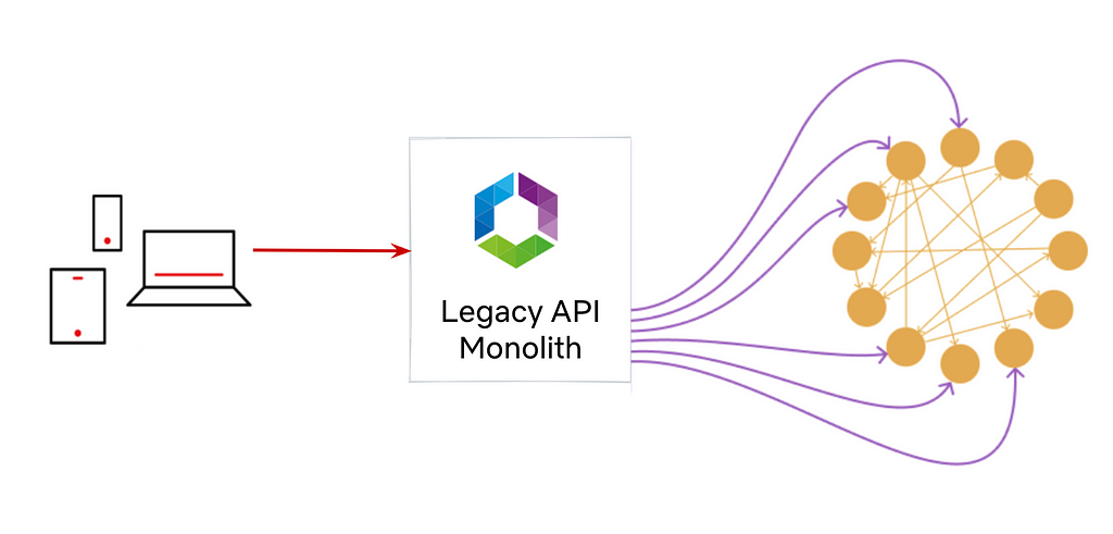
The following architecture diagram shows a virtual machine encompassing the monolithic application and its database.
Challenges
A single virtual machine was quick to set up and inexpensive to operate, but it had considerable shortcomings. The health API was only available in Switzerland, infrastructure maintenance was performed manually, and software deployment was handled manually. Additionally, database backups were done using virtual machine snapshots, uptime monitoring only, and testing was conducted on the developer workstation.
Stage 2: Global and scalable with Kubernetes
At that time, dacadoo made a strategic decision to heavily invest in Kubernetes for managing containerized workloads on a global scale. As part of this technology rollout, the health score and risk service were migrated to Kubernetes.
Due to the geographically distributed customer base and low latency requirements, three Kubernetes clusters were deployed, one on each continent. The NoSQL database was hosted in proximity to the workload to reduce service latency and keep the migration effort low.
To reduce the operational maintenance, the NoSQL database was integrated as a SaaS offering, and monitoring was centralized using Datadog.
All cloud infrastructure was provisioned exclusively with Terraform, covering the Kubernetes cluster, NoSQL database , and integration with GitLab and Datadog.
dacadoo containerized the API service and used Gitlab continuous integration and continuous deployment (CI/CD) pipelines to deploy multiple environments and clusters on a global hyperscaler.
In retrospect, this was a typical replatform modernization project from virtual machine to Kubernetes, with a high level of automation and a SaaS-first approach.
The following diagram is the architecture for the container solution with managed NoSQL database.
Challenges
The service faced several challenges, including increased costs from deploying three regional Kubernetes clusters across three environments, resulting in 27 cluster nodes and additional expenses from managing NoSQL database SaaS instances for each cluster. The complexity of CI/CD pipelines for multi-environment multi-cluster deployments added to the difficulty. Significant operational effort was required to keep infrastructure and Kubernetes components up to date.
Stage 3: Operational excellence with serverless
The Kubernetes-based architecture met the requirements, but some features in the dacadoo API service backlog needed to fit better with the application architecture at the time.
This was the right moment to take a holistic view of the infrastructure and software architecture and refactor the solution according to the latest AWS technologies and best practices, the next frontier for dacadoo’s engineering team.
Solution requirements
Requirements for the solution refactoring were as follows:
Keep the functionality of the API unmodified
Constrain data processing to a region of choice for compliance with local data protection laws
Avoid weekly patch cycles by exclusively using managed serverless services
Reduce costs by choosing services with a pay-as-you-go billing model
Delegate authentication to a dedicated service
Use an established web framework with an extensive ecosystem
Refactoring the apps
The API service has two components: a developer portal and the health score and risk calculations API. The database is only required for API keys, algorithm parameters, quotas, and usage statistics. Health data is processed regionally by the compute layer but not persisted, opening the door for a distributed database: Amazon DynamoDB global tables is the perfect fit for the solution. Writes are distributed to all connected Regions, whereas reads are local, providing low latency for complying with dacadoo service level agreements (SLAs).
The developer portal is a web UI with API documentation and API key management features. AWS Lambda is a great fit because it scales automatically and has a pay-per-request billing model.
The health and risk API uses algorithms implemented in the C programming language for short bursting, compute-intense simulations. These calls are wrapped by a REST API using the Python FastAPI framework. These characteristics make AWS Lambda a great fit.
Serverless architecture
HTTP requests are routed to the Lambda functions using Amazon API Gateway with AWS WAF for protection from malicious requests and attacks. Static assets are served from an Amazon Simple Storage Service (Amazon S3) bucket through API Gateway. The additional features of Amazon CloudFront aren’t required, and Amazon S3 reduces the complexity.
Amazon Route 53 provides a powerful feature known as latency-based routing, which allows it to direct DNS queries to the endpoint that offers the lowest latency for the requester.
This feature provides Regional high availability for API users without data processing location requirements. Alternatively, the user can call specific Regional endpoints to make sure requests are processed in the desired Region.
API authorization is HTTP header-based and is performed in the application with data stored in Amazon DynamoDB.
The following diagram is the architecture for a geo-redundant fully serverless solution.
With a dacadoo SRE team proficient in Python, they opted for Pulumi for its advanced features such as programming language flow control constructs, powerful configuration capabilities, and multi-cloud support.
For continuous integration, GitLab CI compiles the algorithm library, tests the FastAPI applications and packages everything. The application deployment is just an update of the AWS Lambda, a simple and reliable workflow.
Summary
The solution evolved from a managed infrastructure setup, where the customer held most of the responsibility, to an AWS managed service architecture.
Infrastructure provisioning evolved from manual, error-prone processes to powerful code-driven workflows in Pulumi. The SRE needed to enhance their software engineering skills to adopt Pulumi, transitioning from configuration-based approaches to designing and maintaining an infrastructure code base using object-oriented Python. This was part of dacadoo’s investment in the SRE team and broader modernization efforts. The serverless architecture enabled a GitOps engineering culture focused on productivity.
The transformation maximized scalability and availability while reducing costs and operational effort:
Virtual machine
Scalability: Low
Availability: Best effort
Infrastructure costs: Low
Maintenance effort: High
Kubernetes
Scalability: High
Availability: 99.95%
Infrastructure costs: High
Maintenance effort: Medium
Serverless
Scalability: Very high
Availability: 99.999% (with failover to another AWS Region)
Infrastructure costs: Low
Maintenance effort: Very low
The global redundancy elevates availability to an impressive 99.999% while keeping the costs low.
Conclusion
Migrating from a virtual machine to Kubernetes and ultimately to AWS Lambda demonstrates the progression of cloud engineering toward enhanced efficiency and scalability.
Each step in this journey reduced the complexity of managing resources while increasing flexibility and automation. Transitioning dacadoo’s API service to a fully serverless, geo-redundant architecture not only advanced the platform but also upskilled engineers, maintained a lean SRE team, and kept infrastructure costs low. Get started with your own AWS serverless solution.
Amazon Managed Streaming for Apache Kafka (Amazon MSK) now offers a new broker type called Express brokers. It’s designed to deliver up to 3 times more throughput per broker, scale up to 20 times faster, and reduce recovery time by 90% compared to Standard brokers running Apache Kafka. Express brokers come preconfigured with Kafka best practices by default, support Kafka APIs, and provide the same low latency performance that Amazon MSK customers expect, so you can continue using existing client applications without any changes. Express brokers provide straightforward operations with hands-free storage management by offering unlimited storage without pre-provisioning, eliminating disk-related bottlenecks. To learn more about Express brokers, refer to Introducing Express brokers for Amazon MSK to deliver high throughput and faster scaling for your Kafka clusters.
Creating a new cluster with Express brokers is straightforward, as described in Amazon MSK Express brokers. However, if you have an existing MSK cluster, you need to migrate to a new Express based cluster. In this post, we discuss how you should plan and perform the migration to Express brokers for your existing MSK workloads on Standard brokers. Express brokers offer a different user experience and a different shared responsibility boundary, so using them on an existing cluster is not possible. However, you can use Amazon MSK Replicator to copy all data and metadata from your existing MSK cluster to a new cluster comprising of Express brokers.
MSK Replicator offers a built-in replication capability to seamlessly replicate data from one cluster to another. It automatically scales the underlying resources, so you can replicate data on demand without having to monitor or scale capacity. MSK Replicator also replicates Kafka metadata, including topic configurations, access control lists (ACLs), and consumer group offsets.
In the following sections, we discuss how to use MSK Replicator to replicate the data from a Standard broker MSK cluster to an Express broker MSK cluster and the steps involved in migrating the client applications from the old cluster to the new cluster.
Planning your migration
Migrating from Standard brokers to Express brokers requires thorough planning and careful consideration of various factors. In this section, we discuss key aspects to address during the planning phase.
Assessing the source cluster’s infrastructure and needs
It’s crucial to evaluate the capacity and health of the current (source) cluster to make sure it can handle additional consumption during migration, because MSK Replicator will retrieve data from the source cluster. Key checks include:
CPU utilization – The combined CPU User and CPU System utilization per broker should remain below 60%.
Network throughput – The cluster-to-cluster replication process adds extra egress traffic, because it might need to replicate the existing data based on business requirements along with the incoming data. For instance, if the ingress volume is X GB/day and data is retained in the cluster for 2 days, replicating the data from the earliest offset would cause the total egress volume for replication to be 2X GB. The cluster must accommodate this increased egress volume.
Let’s take an example where in your existing source cluster you have an average data ingress of 100 MBps and peak data ingress of 400 MBps with retention of 48 hours. Let’s assume you have one consumer of the data you produce to your Kafka cluster, which means that your egress traffic will be same compared to your ingress traffic. Based on this requirement, you can use the Amazon MSK sizing guide to calculate the broker capacity you need to safely handle this workload. In the spreadsheet, you will need to provide your average and maximum ingress/egress traffic in the cells, as shown in the following screenshot. Because you need to replicate all the data produced in your Kafka cluster, the consumption will be higher than the regular workload. Taking this into account, your overall egress traffic will be at least twice the size of your ingress traffic. However, when you run a replication tool, the resulting egress traffic will be higher than twice the ingress because you also need to replicate the existing data along with the new incoming data in the cluster. In the preceding example, you have an average ingress of 100 MBps and you retain data for 48 hours, which means that you have a total of approximately 18 TB of existing data in your source cluster that needs to be copied over on top of the new data that’s coming through. Let’s further assume that your goal for the replicator is to catch up in 30 hours. In this case, your replicator needs to copy data at 260 MBps (100 MBps for ingress traffic + 160 MBps (18 TB/30 hours) for existing data) to catch up in 30 hours. The following figure illustrates this process. Therefore, in the sizing guide’s egress cells, you need to add an additional 260 MBps to your average data out and peak data out to estimate the size of the cluster you should provision to complete the replication safely and on time. Replication tools act as a consumer to the source cluster, so there is a chance that this replication consumer can consume higher bandwidth, which can negatively impact the existing application client’s produce and consume requests. To control the replication consumer throughput, you can use a consumer-side Kafka quota in the source cluster to limit the replicator throughput. This makes sure that the replicator consumer will throttle when it goes beyond the limit, thereby safeguarding the other consumers. However, if the quota is set too low, the replication throughput will suffer and the replication might never end. Based on the preceding example, you can set a quota for the replicator to be at least 260 MBps, otherwise the replication will not finish in 30 hours.
Volume throughput – Data replication might involve reading from the earliest offset (based on business requirement), impacting your primary storage volume, which in this case is Amazon Elastic Block Store (Amazon EBS). The VolumeReadBytes and VolumeWriteBytes metrics should be checked to make sure the source cluster volume throughput has additional bandwidth to handle any additional read from the disk. Depending on the cluster size and replication data volume, you should provision storage throughput in the cluster. With provisioned storage throughput, you can increase the Amazon EBS throughput up to 1000 MBps depending on the broker size. The maximum volume throughput can be specified depending on broker size and type, as mentioned in Manage storage throughput for Standard brokers in a Amazon MSK cluster. Based on the preceding example, the replicator will start reading from the disk and the volume throughput of 260 MBps will be shared across all the brokers. However, existing consumers can lag, which will cause reading from the disk, thereby increasing the storage read throughput. Also, there is storage write throughput due to incoming data from the producer. In this scenario, enabling provisioned storage throughput will increase the overall EBS volume throughput (read + write) so that existing producer and consumer performance doesn’t get impacted due to the replicator reading data from EBS volumes.
Balanced partitions – Make sure partitions are well-distributed across brokers, with no skewed leader partitions.
Depending on the assessment, you might need to vertically scale up or horizontally scale out the source cluster before migration.
Assessing the target cluster’s infrastructure and needs
Use the same sizing tool to estimate the size of your Express broker cluster. Typically, fewer Express brokers might be needed compared to Standard brokers for the same workload because depending on the instance size, Express brokers allow up to three times more ingress throughput.
Configuring Express Brokers
Express brokers employ opinionated and optimized Kafka configurations, so it’s important to differentiate between configurations that are read-only and those that are read/write during planning. Read/write broker-level configurations should be configured separately as a pre-migration step in the target cluster. Although MSK Replicator will replicate most topic-level configurations, certain topic-level configurations are always set to default values in an Express cluster: replication-factor, min.insync.replicas, and unclean.leader.election.enable. If the default values differ from the source cluster, these configurations will be overridden.
As part of the metadata, MSK Replicator also copies certain ACL types, as mentioned in Metadata replication. It doesn’t explicitly copy the write ACLs except the deny ones. Therefore, if you’re using SASL/SCRAM or mTLS authentication with ACLs rather than AWS Identity and Access Management (IAM) authentication, write ACLs need to be explicitly created in the target cluster.
Client connectivity to the target cluster
Deployment of the target cluster can occur within the same virtual private cloud (VPC) or a different one. Consider any changes to client connectivity, including updates to security groups and IAM policies, during the planning phase.
Migration strategy: All at once vs. wave
Two migration strategies can be adopted:
All at once – All topics are replicated to the target cluster simultaneously, and all clients are migrated at once. Although this approach simplifies the process, it generates significant egress traffic and involves risks to multiple clients if issues arise. However, if there is any failure, you can roll back by redirecting the clients to use the source cluster. It’s recommended to perform the cutover during non-business hours and communicate with stakeholders beforehand.
Wave – Migration is broken into phases, moving a subset of clients (based on business requirements) in each wave. After each phase, the target cluster’s performance can be evaluated before proceeding. This reduces risks and builds confidence in the migration but requires meticulous planning, especially for large clusters with many microservices.
Each strategy has its pros and cons. Choose the one that aligns best with your business needs. For insights, refer to Goldman Sachs’ migration strategy to move from on-premises Kafka to Amazon MSK.
Cutover plan
Although MSK Replicator facilitates seamless data replication with minimal downtime, it’s essential to devise a clear cutover plan. This includes coordinating with stakeholders, stopping producers and consumers in the source cluster, and restarting them in the target cluster. If a failure occurs, you can roll back by redirecting the clients to use the source cluster.
Schema registry
When migrating from a Standard broker to an Express broker cluster, schema registry considerations remain unaffected. Clients can continue using existing schemas for both producing and consuming data with Amazon MSK.
Solution overview
In this setup, two Amazon MSK provisioned clusters are deployed: one with Standard brokers (source) and the other with Express brokers (target). Both clusters are located in the same AWS Region and VPC, with IAM authentication enabled. MSK Replicator is used to replicate topics, data, and configurations from the source cluster to the target cluster. The replicator is configured to maintain identical topic names across both clusters, providing seamless replication without requiring client-side changes.
During the first phase, the source MSK cluster handles client requests. Producers write to the clickstream topic in the source cluster, and a consumer group with the group ID clickstream-consumer reads from the same topic. The following diagram illustrates this architecture.
When data replication to the target MSK cluster is complete, we need to evaluate the health of the target cluster. After confirming the cluster is healthy, we need to migrate the clients in a controlled manner. First, we need to stop the producers, reconfigure them to write to the target cluster, and then restart them. Then, we need to stop the consumers after they have processed all remaining records in the source cluster, reconfigure them to read from the target cluster, and restart them. The following diagram illustrates the new architecture.
After verifying that all clients are functioning correctly with the target cluster using Express brokers, we can safely decommission the source MSK cluster with Standard brokers and the MSK Replicator.
Deployment Steps
In this section, we discuss the step-by-step process to replicate data from an MSK Standard broker cluster to an Express broker cluster using MSK Replicator and also the client migration strategy. For the purpose of the blog, “all at once” migration strategy is used.
Provision the MSK cluster
Download the AWS CloudFormationtemplate to provision the MSK cluster. Deploy the following in us-east-1 with stack name as migration.
This will create the VPC, subnets, and two Amazon MSK provisioned clusters: one with Standard brokers (source) and another with Express brokers (target) within the VPC configured with IAM authentication. It will also create a Kafka client Amazon Elastic Compute Cloud (Amazon EC2) instance where from we can use the Kafka command line to create and view Kafka topics and produce and consume messages to and from the topic.
Configure the MSK client
On the Amazon EC2 console, connect to the EC2 instance named migration-KafkaClientInstance1 using Session Manager, a capability of AWS Systems Manager.
After you log in, you need to configure the source MSK cluster bootstrap address to create a topic and publish data to the cluster. You can get the bootstrap address for IAM authentication from the details page for the MSK cluster (migration-standard-broker-src-cluster) on the Amazon MSK console, under View Client Information. You also need to update the producer.properties and consumer.properties files to reflect the bootstrap address of the standard broker cluster.
sudo su - ec2-user

export BS_SRC=<<SOURCE_MSK_BOOTSTRAP_ADDRESS>>
sed -i "s/BOOTSTRAP_SERVERS_CONFIG=/BOOTSTRAP_SERVERS_CONFIG=${BS_SRC}/g" producer.properties
sed -i "s/bootstrap.servers=/bootstrap.servers=${BS_SRC}/g" consumer.properties
Create a topic
Create a clickstream topic using the following commands:
Keep the producer and consumer running. If not interrupted, the producer and consumer will run for 60 minutes before it exits. The -rf parameter controls how long the producer and consumer will run.
Create an MSK replicator
To create an MSK replicator, complete the following steps:
On the Amazon MSK console, choose Replicators in the navigation pane.
Choose Create replicator.
In the Replicator details section, enter a name and optional description.
In the Source cluster section, provide the following information:
For Cluster region, choose us-east-1.
For MSK cluster, enter the MSK cluster Amazon Resource Name (ARN) for the Standard broker.
After the source cluster is selected, it automatically selects the subnets associated with the primary cluster and the security group associated with the source cluster. You can also select additional security groups.
Make sure that the security groups have outbound rules to allow traffic to your cluster’s security groups. Also make sure that your cluster’s security groups have inbound rules that accept traffic from the replicator security groups provided here.
In the Target cluster section, for MSK cluster¸ enter the MSK cluster ARN for the Express broker.
After the target cluster is selected, it automatically selects the subnets associated with the primary cluster and the security group associated with the source cluster. You can also select additional security groups.
Now let’s provide the replicator settings.
In the Replicator settings section, provide the following information:
For the purpose of the example, we have kept the topics to replicate as a default value that would replicate all topics from primary to secondary cluster.
For Replicator starting position, we configure it to replicate from the earliest offset, so that we can get all the events from the start of the source topics.
To configure the topic name in the secondary cluster as identical to the primary cluster, we select Keep the same topic names for Copy settings. This makes sure that the MSK clients don’t need to add a prefix to the topic names.
For this example, we keep the Consumer Group Replication setting as default (make sure it’s enabled to allow redirected clients resume processing data from the last processed offset).
We set Target Compression type as None.
The Amazon MSK console will automatically create the required IAM policies. If you’re deploying using the AWS Command Line Interface (AWS CLI), SDK, or AWS CloudFormation, you have to create the IAM policy and use it as per your deployment process.
Choose Create to create the replicator.
The process will take around 15–20 minutes to deploy the replicator. When the MSK replicator is running, this will be reflected in the status.
Monitor replication
When the MSK replicator is up and running, monitor the MessageLag metric. This metric indicates how many messages are yet to be replicated from the source MSK cluster to the target MSK cluster. The MessageLag metric should come down to 0.
Migrate clients from source to target cluster
When the MessageLag metric reaches 0, it indicates that all messages have been replicated from the source MSK cluster to the target MSK cluster. At this stage, you can cut over client applications from the source to the target cluster. Before initiating this step, confirm the health of the target cluster by reviewing the Amazon MSK metrics in Amazon CloudWatch and making sure that the client applications are functioning properly. Then complete the following steps:
Stop the producers writing data to the source (old) cluster with Standard brokers and reconfigure them to write to the target (new) cluster with Express brokers.
Before migrating the consumers, make sure that the MaxOffsetLag metric for the consumers has dropped to 0, confirming that they have processed all existing data in the source cluster.
When this condition is met, stop the consumers and reconfigure them to read from the target cluster.
The offset lag happens if the consumer is consuming slower than the rate the producer is producing data. The flat line in the following metric visualization shows that the producer has stopped producing to the source cluster while the consumer attached to it continues to consume the existing data and eventually consumes all the data, therefore the metric goes to 0.
Now you can update the bootstrap address in properties and consumer.properties to point to the target Express based MSK cluster. You can get the bootstrap address for IAM authentication from the MSK cluster (migration-express-broker-dest-cluster) on the Amazon MSK console under View Client Information.
export BS_TGT=<<TARGET_MSK_BOOTSTRAP_ADDRESS>>
sed -i "s/BOOTSTRAP_SERVERS_CONFIG=.*/BOOTSTRAP_SERVERS_CONFIG=${BS_TGT}/g" producer.properties
sed -i "s/bootstrap.servers=.*/bootstrap.servers=${BS_TGT}/g" consumer.properties
Run the clickstream producer to generate events in the clickstream topic:
We can see that the producers and consumers are now producing and consuming to the target Express based MSK cluster. The producers and consumers will run for 60 seconds before they exit.
The following screenshot shows producer-produced messages to the new Express based MSK cluster for 60 seconds.
Migrate stateful applications
Stateful applications such as Kafka Streams, KSQL, Apache Spark, and Apache Flink use their own checkpointing mechanisms to store consumer offsets instead of relying on Kafka’s consumer group offset mechanism. When migrating topics from a source cluster to a target cluster, the Kafka offsets in the source will differ from those in the target. As a result, migrating a stateful application along with its state requires careful consideration, because the existing offsets are incompatible with the target cluster’s offsets. Before migrating stateful applications, it is crucial to stop producers and make sure that consumer applications have processed all data from the source MSK cluster.
Migrate Kafka Streams and KSQL applications
Kafka Streams and KSQL store consumer offsets in internal changelog topics. It is advisable not to replicate these internal changelog topics to the target MSK cluster. Instead, the Kafka Streams application should be configured to start from the earliest offset of the source topics in the target cluster. This allows the state to be rebuilt. However, this method results in duplicate processing, because all the data in the topic is reprocessed. Therefore, the target destination (such as a database) must be idempotent to handle these duplicates effectively.
Express brokers don’t allow configuring segment.bytes to optimize performance. Therefore, the internal topics need to be manually created before the Kafka Streams application is migrated to the new Express based cluster. For more information, refer to Using Kafka Streams with MSK Express brokers and MSK Serverless.
Migrate Spark applications
Spark stores offsets in its checkpoint location, which should be a file system compatible with HDFS, such as Amazon Simple Storage Service (Amazon S3). After migrating the Spark application to the target MSK cluster, you should remove the checkpoint location, causing the Spark application to lose its state. To rebuild the state, configure the Spark application to start processing from the earliest offset of the source topics in the target cluster. This will lead to re-processing all the data from the start of the topic and therefore will generate duplicate data. Consequently, the target destination (such as a database) must be idempotent to effectively handle these duplicates.
Migrate Flink applications
Flink stores consumer offsets within the state of its Kafka source operator. When checkpoints are completed, the Kafka source commits the current consuming offset to provide consistency between Flink’s checkpoint state and the offsets committed on Kafka brokers. Unlike other systems, Flink applications don’t rely on the __consumer_offsets topic to track offsets; instead, they use the offsets stored in Flink’s state.
During Flink application migration, one approach is to start the application without a Savepoint. This approach discards the entire state and reverts to reading from the last committed offset of the consumer group. However, this prevents the application from accurately rebuilding the state of downstream Flink operators, leading to discrepancies in computation results. To address this, you can either avoid replicating the consumer group of the Flink application or assign a new consumer group to the application when restarting it in the target cluster. Additionally, configure the application to start reading from the earliest offset of the source topics. This enables re-processing all data from the source topics and rebuilding the state. However, this method will result in duplicate data, so the target system (such as a database) must be idempotent to handle these duplicates effectively.
Alternatively, you can reset the state of the Kafka source operator. Flink uses operator IDs (UIDs) to map the state to specific operators. When restarting the application from a Savepoint, Flink matches the state to operators based on their assigned IDs. It is recommended to assign a unique ID to each operator to enable seamless state restoration from Savepoints. To reset the state of the Kafka source operator, change its operator ID. Passing the operator ID as a parameter in a configuration file can simplify this process. Restart the Flink application with parameter --allowNonRestoredState (if you are running self-managed Flink). This will reset only the state of the Kafka source operator, leaving other operator states unaffected. As a result, the Kafka source operator resumes from the last committed offset of the consumer group, avoiding full reprocessing and state rebuilding. Although this might still produce some duplicates in the output, it results in no data loss. This approach is applicable only when using the DataStream API to build Flink applications.
Conclusion
Migrating from a Standard broker MSK cluster to an Express broker MSK cluster using MSK Replicator provides a seamless, efficient transition with minimal downtime. By following the steps and strategies discussed in this post, you can take advantage of the high-performance, cost-effective benefits of Express brokers while maintaining data consistency and application uptime.
Ready to optimize your Kafka infrastructure? Start planning your migration to Amazon MSK Express brokers today and experience improved scalability, speed, and reliability. For more details, refer to the Amazon MSK Developer Guide.
About the Author
Subham Rakshit is a Senior Streaming Solutions Architect for Analytics at AWS based in the UK. He works with customers to design and build streaming architectures so they can get value from analyzing their streaming data. His two little daughters keep him occupied most of the time outside work, and he loves solving jigsaw puzzles with them. Connect with him on LinkedIn.
Based in northern Brazil, TO HOST Data Centers provides regional cloud services with a focus on cloud computing, colocation, and infrastructure management. With 35 suppliers and partners and over 5,000 monitored assets, their mission is to provide innovative IT infrastructure products and services with a high level of proficiency, in order to meet the high standards required by their clients and partners. To do this, they need to monitor internal applications, data center assets, devices, and customer environments, ensuring high availability and optimal performance.
The challenge:
TO HOST’s monitoring environment included a standalone server (Zabbix, FrontEnd, Database) with the following:
Hosts: ~600
Itens/Metrics: ~90.000
Average period for history table: 45~60 days
Average period for trends table: 365 days
Average period for events table: 365 days
3 Internal Proxies
8 Client Proxies
~30 External Active Agents
TO HOST needed a clean installation of Zabbix Server and Zabbix Proxy version 7.0.x on separate virtual machines with an updated operating system (Oracle 9), plus a migration of the current monitoring environment database to the new version, while preserving history and data integrity.
Their production servers were outdated, featuring a CentOS 7 version that was originally installed with Zabbix version 5.2.x and updated to version 6.0.x in 2022. The migration needed to retain historical data and ensure compatibility with Zabbix 7.0.x, while keeping service interruptions to a minimum.
A number of risks were anticipated and planned for – during the data migration process, it was understood that there may be failures in migrating the database due to version incompatibility and that there was a distinct possibility of collection failures that would require corrections after migration, if any data sources were not properly mapped.
All graphs needed to be reviewed and optimized to take advantage of the new widget models and improvements in Zabbix 7.0. Due to the changes in data sources (and because of the migration to a new operating system and a new version of the Zabbix Server) there was potential version incompatibility.
Directories containing custom scripts and images were mapped and files were copied in order to ensure integrity, and the TO HOST team was prepared for possible service interruptions during the upgrade process, standing ready to notify users about the planned maintenance and creating procedures to minimize the impact.
The solution:
Step one was to make sure that the change to Zabbix 7.0 was appropriately planned. A change schedule was created, and all relevant stakeholders were notified of the operation. A virtualized environment was then set up on Oracle 9, in order to guarantee a clean installation.
Once that was done, Zabbix 7.0 was installed, keeping in mind that the imported database could not exist on the new server. Next up was a full backup and the cloning of the database for integrity validation pre-migration. At this point, the To Host team stopped the data collection service, started the backup, and started restore.
From that point, it became a simple matter of carrying out automated database versioning and data source mapping corrections. The data mapping during the Zabbix 7.0 migration involved updating the database structure to meet the new version’s requirements, such as changes to MySQL instances, fields, and storage formats.
Data mapping in the Zabbix migration process involved the following:
Database Version: During migration, the database structure changed to align with the requirements of Zabbix 7.0. This included different versioning of MySQL instances, as well as modifications to fields, tables, and storage formats within the database.
Import and Update Process: The legacy database (version 6) was exported and then imported into the new Zabbix 7.0 installation. During the process, Zabbix ran automatic update scripts to convert the old database into the new format.
Data Sources: Each item monitored in Zabbix was associated with a unique key (item key) that defined how data was collected and processed. No changes were identified in this process.
Tools and Validations: Mapping validation was performed during the import/restore process, where error logs indicated inconsistencies. During testing, inconsistencies were found in the validation, requiring a command to update the keys replicated on the migration.
Data collection services were then restarted, and all stakeholders were notified of the completion of the change.
The results:
Zabbix 7.0’s new dashboards and improved visual configuration have increased the satisfaction of internal customers, while having a tangible impact on operational efficiency and customer satisfaction.
The implementation and management of Zabbix 7.0 has enhanced the continuous visibility and integrity of TO HOST’s IT systems, enabling real-time monitoring and alerting, facilitating proactive issue resolution, and guaranteeing optimal infrastructure performance.
Many users have noted that the asynchronous polling method used in Zabbix 7.0 significantly reduces the time taken for metric collection. This allows for faster incident detection and resolution in TO HOST’s critical environment, while the addition of multi-factor authentication and improved access controls has helped to enhance security in monitoring environments and keep cyber threats at bay.
TO HOST’s future plans include exploring advanced Zabbix 7.0 features and continuous performance monitoring. A roadmap is already in place to leverage the additional automation and security enhancements that Zabbix 7.0 can provide.
Google Analytics 4 (GA4) provides valuable insights into user behavior across websites and apps. But what if you need to combine GA4 data with other sources or perform deeper analysis? That’s where Amazon Redshift and Amazon AppFlow come in. Amazon AppFlow bridges the gap between Google applications and Amazon Redshift, empowering organizations to unlock deeper insights and drive data-informed decisions. In this post, we show you how to establish the data ingestion pipeline between Google Analytics 4, Google Sheets, and an Amazon Redshift Serverless workgroup.
Amazon AppFlow is a fully managed integration service that you can use to securely transfer data from software as a service (SaaS) applications, such as Google BigQuery, Salesforce, SAP, HubSpot, and ServiceNow, to Amazon Web Services (AWS) services such as Amazon Simple Storage Service (Amazon S3) and Amazon Redshift, in just a few clicks. With Amazon AppFlow, you can run data flows at nearly any scale and at the frequency you choose—on a schedule, in response to a business event, or on demand. You can configure data transformation capabilities such as filtering and validation to generate rich, ready-to-use data as part of the flow itself, without additional steps. Amazon AppFlow automatically encrypts data in motion, and allows you to restrict data from flowing over the public internet for SaaS applications that are integrated with AWS PrivateLink, reducing exposure to security threats.
Amazon Redshift is a fast, scalable, and fully managed cloud data warehouse that allows you to process and run your complex SQL analytics workloads on structured and semi-structured data. It also helps you securely access your data in operational databases, data lakes, or third-party datasets with minimal movement or copying of data. Tens of thousands of customers use Amazon Redshift to process large amounts of data, modernize their data analytics workloads, and provide insights for their business users.
Prerequisites
Before starting this walkthrough, you need to have the following prerequisites in place:
The following architecture shows how Amazon AppFlow can transform and move data from SaaS applications to processing and storage destinations. Three sections appear from left to right in the diagram: Source, Move, Target. These sections are described in the following section.
Source – The leftmost section on the diagram represents different applications acting as a source, including Google Analytics, Google Sheets, and Google BigQuery.
Move – The middle section is labeled Amazon AppFlow. The section contains boxes that represent Amazon AppFlow operations such as Mask Fields, Map Fields, Merge Fields, Filter Data, and others. In this post, we focus on setting up the data movement using Amazon AppFlow and filtering data based on start date. The other transformation operations such as mapping, masking, and merging fields are not covered in this post.
Destination – The section on the right of the diagram is labeled Destination and represents targets such as Amazon Redshift and Amazon S3. In this psot, we primarily focus on Amazon Redshift as the destination.
Application configuration in Google Cloud Platform
Amazon AppFlow requires OAuth 2.0 for authentication. You need to create an OAuth 2.0 client ID, which Amazon AppFlow uses when requesting an OAuth 2.0 access token. To create an OAuth 2.0 client ID in the Google Cloud Platform console, follow these steps:
If the APIs & Services page isn’t already open, choose the menu icon on the upper left and select APIs & Services.
In the navigation pane, choose Credentials.
Choose CREATE CREDENTIALS, then choose OAuth client ID, as shown in the following screenshot.
Select the application type Web application, enter the name demo-google-aws, and provide URIs for Authorized JavaScript originshttps://console.aws.amazon.com. For Authorized redirect URIs, add https://us-east-1.console.aws.amazon.com/appflow/oauth. Choose SAVE, as shown in the following screenshot.
The OAuth client ID is now created. Select demo-google-aws.
Under Additional information, as shown in the following screenshot, note down the Client ID and Client secret.
Data ingestion from Google Analytics 4 to Amazon Redshift
In this section, you configure Amazon AppFlow to set up a connection between Google Analytics 4 and Amazon Redshift for data migration. This procedure can be classified into the following steps:
In the navigation pane on the left, choose Connections.
On the Manage connections page, for Connectors, choose Google Analytics 4.
Choose Create connection.
In the Connect to Google Analytics 4 window, enter the following information. For Client ID, enter the client ID of the OAuth 2.0 client ID in your Google Cloud project created in the previous section. For Client secret, enter the client secret of the OAuth 2.0 client ID in your Google Cloud project created in the previous section.
(Optional) under Data encryption, choose Customize encryption settings (advanced) if you want to encrypt your data with a customer managed key in AWS Key Management Service (AWS KMS). By default, Amazon AppFlow encrypts your data with an AWS KMS key that AWS creates, uses, and manages for you. Choose this option if you want to encrypt your data with your own AWS KMS key instead.
The following screenshot shows the Connect to Google Analytics 4 window.
If you want to use an AWS KMS key from the current AWS account, select this key under Choose an AWS KMS key. If you want to use an AWS KMS key from a different AWS account, enter the Amazon Resource Name (ARN) for that key:
For Connection name, enter a name for your connection
Choose Continue
In the window that appears, sign in to your Google account and grant access to Amazon AppFlow
On the Manage connections page, your new connection appears in the Connections table. When you create a flow that uses Google Analytics 4 as the data source, you can select this connection.
Create an IAM role for Amazon AppFlow integration with Amazon Redshift
You can use Amazon AppFlow to transfer data from supported sources into your Amazon Redshift databases. You need an IAM role because Amazon AppFlow needs authorization to access Amazon Redshift using an Amazon Redshift Data API.
Select the JSON tab and paste in the following policy. Amazon AppFlow needs the following permissions to gain access and run SQL statements with the Amazon Redshift database.
Choose Next, provide the Policy name as appflow-redshift-policy, Description as appflow redshift policy, and choose Create policy.
In the navigation pane, choose Roles and Create role. Choose Custom trust policy and paste in the following. Choose Next. This trust policy grants Amazon AppFlow the ability to assume the role for Amazon AppFlow to access and process data.
Search for policy appflow-redshift-policy, check the box next to it, and choose Next.
Provide the role name appflow-redshift-access-role and Description and choose Create role.
Set up Amazon AppFlow connection for Amazon Redshift
To set up an Amazon AppFlow connection for Amazon Redshift, follow these steps:
On the Amazon AppFlow console, in the navigation pane, choose Connectors, select Amazon Redshift, and choose Create connection.
Enter the connection name appflow-redshift-connection. You can either use Amazon Redshift provisioned or Amazon Redshift Serverless, but in this example we are using Amazon Redshift Serverless. Select Amazon Redshift Serverless and enter the workgroup name and database name.
Choose the S3 bucket and enter the bucket prefix.
For Amazon S3 access, select the IAM role attached to the Redshift cluster or namespace during the creation of the Redshift cluster. Additionally, for the Amazon Redshift Data API, choose the IAM role appflow-redshift-access-role created in the previous section and then choose
Set up a table and permission in Amazon Redshift
To set up table and permission in Amazon Redshift, follow these steps:
On the Amazon Redshift console, choose Query editor v2 in Explorer.
Connect to your existing Redshift cluster or Amazon Redshift Serverless workgroup.
Create a table with the following Data Definition Language (DDL).
create table public.stg_ga4_daily_summary

(

event_date date,

region varchar(255),

country varchar(255),

city varchar(255),

deviceCategory varchar(255),

deviceModel varchar(255),

browser varchar(255),

active_users INTEGER,

new_users integer,

total_revenue  NUMERIC(18,2)

);
The following screenshot shows the successful creation of this table in Amazon Redshift:
The following step is only applicable to Amazon Redshift Serverless. If you are using a Redshift provisioned cluster, you can skip this step.
Grant the permissions on the table to the IAM user used by Amazon AppFlow to load data into Amazon Redshift Serverless, for example, appflow-redshift-access-role.
GRANT INSERT ON TABLE public.stg_ga4_daily_summary TO "IAMR:appflow-redshift-access-role";
Create data flow in Amazon AppFlow
To create a data flow in Amazon AppFlow, follow these steps:
On the Amazon AppFlow console, choose Flows and select Amazon Redshift. Choose Create flow and enter the flow name and the flow description, as shown in the following screenshot.
In Source name, choose Google Analytics 4. Choose the Google Analytics 4 connection.
Select the Google Analytics 4 object, then choose Amazon Redshift as the destination, selecting the public schema and stg_ga4_daily_summary table in your Redshift instance.
For Flow trigger, choose Run on demand and choose Next, as shown in the following screenshot.
You can run the flow on schedule to pull either full or incremental data refresh. For more information, see Schedule-triggered flows.
Select Manually map fields. From the Source field name dropdown menu, select the attribute date, and from the Destination field name, select event_date and choose Map fields, as shown in the following screenshot.
Repeat the previous step (step 5) for the following attributes and then choose Next. The following screenshot shows the mapping.
The Google Analytics API provides various dimensions and metrics for reporting purposes. Refer to API Dimensions & Metrics for details.
In Field name, enter the filter start_end_date and choose Next, as shown in the following screenshot. The Amazon AppFlow date filter supports both a start date (criteria1) and an end date (criteria2) to define the desired date range for data transfer. We are using the date range because we have sample data created for this range.
Review the configurations and choose Create flow.
Choose Run flow, as shown in the following screenshot, and wait for the flow execution to be completed.
On the Amazon Redshift console, choose Query editor v2 in Explorer.
Connect to your existing Redshift cluster or Amazon Redshift Serverless workgroup.
Enter the following SQL to verify the data in Amazon Redshift.
select * from public.stg_ga4_daily_summary
The screenshot below shows the results loaded into the stg_ga4_daily_summary table.
Data ingestion from Google Sheets to Amazon Redshift
Ingesting data from Google Sheets to Amazon Redshift using Amazon AppFlow streamlines analytics, enabling seamless transfer and deeper insights. In this section, we demonstrate how business users can maintain their business glossary in Google Sheets and integrate that using Amazon AppFlow with Amazon Redshift and get meaningful insights.
For this demo, you can upload the Nation Market segment file to your Google sheet before proceeding to the next steps. These steps show how to configure Amazon AppFlow to set up a connection between Google Sheets and Amazon Redshift for data migration. This procedure can be classified into the following steps:
To create a Google Sheets connection in Amazon AppFlow, follow these steps:
On the Amazon AppFlow console, choose Connectors, select Google Sheets, then choose Create connection.
In the Connect to Google Sheets window, enter the following information. For Client ID, enter the client ID of the OAuth 2.0 client ID in your Google Sheets project. For Client secret, enter the client secret of the OAuth 2.0 client ID in your Google Sheets project.
For Connection name, enter a name for your connection.
(Optional) Under Data encryption, choose Customize encryption settings (advanced) if you want to encrypt your data with a customer managed key in AWS KMS. By default, Amazon AppFlow encrypts your data with an AWS KMS key that AWS creates, uses, and manages for you. Choose this option if you want to encrypt your data with your own AWS KMS key instead.
Choose Connect.
In the window that appears, sign in to your Google account and grant access to Amazon AppFlow.
Set up table and permission in Amazon Redshift
To set up a table and permission in Amazon Redshift, follow these steps:
On the Amazon Redshift console, choose Query editor v2 in Explorer
Connect to your existing Redshift cluster or Amazon Redshift Serverless workgroup
Create a table with the following DDL
create table public.stg_nation_market_segment(
n_nationkey int4 not null,
n_name char(25) not null ,
n_regionkey int4 not null,
n_comment varchar(152) not null,
n_marketsegment varchar(255),
Primary Key(N_NATIONKEY)
) distkey(n_nationkey) sortkey(n_nationkey);
he following steps are only applicable to Amazon Redshift Serverless. If you are using a Redshift provisioned cluster, you can skip this step.
Grant the permissions on the table to the IAM user used by Amazon AppFlow to load data into Amazon Redshift Serverless, for example, appflow-redshift-access-role
GRANT INSERT ON TABLE public.stg_nation_market_segment TO "IAMR:appflow-redshift-access-role";
Create data flow in Amazon AppFlow
On the Amazon AppFlow console, choose Flows and select Google Sheets. Choose Create flow, enter the flow name and flow description, and choose Next.
Select Google Sheets in Source name and choose the Google Sheets connection.
Select the Google Sheets object nation_market_segment#Sheet1.
Choose the Destination name as Amazon Redshift, then select stg_nation_market_segment as your Amazon Redshift object, as shown in the following screenshot.
For Flow trigger, select On demand and choose Next.
You can run the flow on schedule to pull full or incremental data refresh. Read more at Schedule-triggered flows.
Select Manually map fields. From the Source field name dropdown menu, select Map all fields directly. When a dialog box pops up, choose the respective attribute values and choose Map fields, as shown in the following screenshot. Choose Next.
The following screenshot shows the mapping.
On the Add Filters page, choose Next.
On the Review and create page, choose Create flow.
Choose Run flow and wait for the flow execution to finish.
The screenshot below shows the execution details of the flow job.
On the Amazon Redshift console, choose Query editor v2 in Explorer.
Connect to your existing Redshift cluster or Amazon Redshift Serverless workgroup.
Run the following SQL to verify the data in Amazon Redshift.
select * from public.stg_nation_market_segment
The screenshot below shows the results loaded into the stg_nation_market_segment table.
Run the following SQL to prepare a sample dataset in Amazon Redshift.
create table public.customer (
c_custkey int8 not null ,
c_name varchar(25) not null,
c_address varchar(40) not null,
c_nationkey int4 not null,
c_phone char(15) not null,
c_acctbal numeric(12,2) not null,
c_mktsegment char(10) not null,
c_comment varchar(117) not null,
Primary Key(C_CUSTKEY)
) distkey(c_custkey) sortkey(c_custkey);

create table public.lineitem (
l_orderkey int8 not null ,
l_partkey int8 not null,
l_suppkey int4 not null,
l_linenumber int4 not null,
l_quantity numeric(12,2) not null,
l_extendedprice numeric(12,2) not null,
l_discount numeric(12,2) not null,
l_tax numeric(12,2) not null,
l_returnflag char(1) not null,
l_linestatus char(1) not null,
l_shipdate date not null ,
l_commitdate date not null,
l_receiptdate date not null,
l_shipinstruct char(25) not null,
l_shipmode char(10) not null,
l_comment varchar(44) not null,
Primary Key(L_ORDERKEY, L_LINENUMBER)
) distkey(l_orderkey) sortkey(l_shipdate,l_orderkey)  ;

create table public.orders (
o_orderkey int8 not null,
o_custkey int8 not null,
o_orderstatus char(1) not null,
o_totalprice numeric(12,2) not null,
o_orderdate date not null,
o_orderpriority char(15) not null,
o_clerk char(15) not null,
o_shippriority int4 not null,
o_comment varchar(79) not null,
Primary Key(O_ORDERKEY)
) distkey(o_orderkey) sortkey(o_orderdate, o_orderkey) ;
copy lineitem from 's3://redshift-downloads/TPC-H/2.18/10GB/lineitem.tbl' iam_role default delimiter '|' region 'us-east-1';
copy orders from 's3://redshift-downloads/TPC-H/2.18/10GB/orders.tbl' iam_role default delimiter '|' region 'us-east-1';
copy customer from 's3://redshift-downloads/TPC-H/2.18/10GB/customer.tbl' iam_role default delimiter '|' region 'us-east-1';
Run the following SQL to do the data analytics using Google Sheets business data classification in the Amazon Redshift dataset.
select
n_marketsegment,
sum(l_extendedprice * (1 - l_discount)) as revenue
from
public.customer,
public.orders,
public.lineitem,
public.stg_nation_market_segment
where
c_custkey = o_custkey
and l_orderkey = o_orderkey
and c_nationkey = n_nationkey
group by
1
order by
revenue desc;
The screenshot below shows the results from the aggregated query in Amazon Redshift from data loaded using Amazon Appflow.
Clean up
To avoid incurring charges, clean up the resources in your AWS account by completing the following steps:
On the Amazon AppFlow console, in the navigation pane, choose Flows.
From the list of flows, select the flow name created and delete it.
Enter “delete” to delete the flow.
Delete the Amazon Redshift workgroup.
Clean up resources in your Google account by deleting the project that contains the Google BigQuery resources. Follow the documentation to clean up the Google resources.
Conclusion
In this post, we walked you through the process of using Amazon AppFlow to integrate data from Google Ads and Google Sheets. We demonstrated how the complexities of data integration are minimized so you can focus on deriving actionable insights from your data. Whether you’re archiving historical data, performing complex analytics, or preparing data for machine learning, this connector streamlines the process, making it accessible to a broader range of data professionals.
Ritesh Kumar Sinha is an Analytics Specialist Solutions Architect based out of San Francisco. He has helped customers build scalable data warehousing and big data solutions for over 16 years. He loves to design and build efficient end-to-end solutions on AWS. In his spare time, he loves reading, walking, and doing yoga.
Tahir Aziz is an Analytics Solution Architect at AWS. He has worked with building data warehouses and big data solutions for over 13 years. He loves to help customers design end-to-end analytics solutions on AWS. Outside of work, he enjoys traveling and cooking.
Raza Hafeez is a Senior Product Manager at Amazon Redshift. He has over 13 years of professional experience building and optimizing enterprise data warehouses and is passionate about enabling customers to realize the power of their data. He specializes in migrating enterprise data warehouses to AWS Modern Data Architecture.
Amit Ghodke is an Analytics Specialist Solutions Architect based out of Austin. He has worked with databases, data warehouses and analytical applications for the past 16 years. He loves to help customers implement analytical solutions at scale to derive maximum business value.
AWS DMS is a cloud service that makes it possible to migrate relational databases, data warehouses, NoSQL databases, and other types of data stores. You can use AWS DMS to migrate your data into the Amazon Web Services (AWS) Cloud or between combinations of cloud and on-premises setups.
Today, more than 1 million databases have been migrated using AWS Database Migration Service. AWS DMS helps you migrate your data from one database system to another. And, when migrating between different database engines, AWS DMS SC helps to convert the source database schema and procedures to the target database system.
However, although AWS DMS SC automates many steps in these migrations, certain complex database code elements still require manual intervention, which can extend migration timelines and add cost. This is particularly the case with proprietary system functions or procedures, and data type conversions, which don’t always have direct equivalents in PostgreSQL.
The new generative AI capability in AWS DMS SC is designed to address these challenges by automating some of the most time-intensive schema conversion tasks. Using large language models (LLMs) hosted on Amazon Bedrock, the new capability expands the existing conversion capabilities. It converts code snippets in the source database that were otherwise not supported by traditional rule-based techniques, including complex procedures and functions.
Generative AI–assisted code conversion helps to reduce migration costs and accelerate project timelines. Because AWS DMS SC automates more of the schema conversion process, you can focus on higher value tasks such as refining and optimizing your applications post-migration rather than manually resolving conversion gaps. Our beta customers have already experienced success with these AI-powered features in AWS DMS SC, achieving cost savings and faster migrations.
Let’s find out how it works To demonstrate the ease of using this new generative AI capability, I’ll walk through the schema conversion process in AWS DMS SC. AWS DMS SC simplifies database migration by automatically converting my source database’s structure, including tables, views, stored procedures, functions, and more, to a format compatible with my target database. Any objects that can’t be automatically converted are flagged for manual attention.
After my project is created, I select it, and on the Schema conversion tab, I choose Launch schema conversion. It takes a couple of minutes to launch the conversion tool the first time.
AWS DMS SC with generative AI is an opt-in capability. I first activate the option. On the Settings tab, I turn on Enable Generative AI feature for conversion.
Before diving into the details of the conversion, I would like to get an overall assessment of the migration complexity. I select the schema I want to migrate. Then I select Assess in the menu.
After a few minutes, a high-level Summary is available. The Action items tab has more details. I choose Export results and choose PDF to receive a report to share with my colleagues. The report is generated and available from an S3 bucket.
The summary screen shows the percentage of Database storage objects and Database code objects that can be converted by the rule-based method. That’s 100% and 57% in this example. Let’s see how the generative AI-based conversion will change that.
The PDF contains an executive summary, various statistics about the number of objects to be migrated, the feasibility of conversion with generative AI, and the complexity of the migration.
By reading the report, I learn there is no blocker detected to migrate the stored procedures. I select the stored procedure I want to migrate (PRC_AIML_DEMO6). Then, I select the Actions menu on the source database (the left one) and choose Convert.
After a minute or two, I can read the original procedure code in the left pane and the proposed migrated version on the right panel.
The summary screen has been updated. Now, it shows that 100 percent of the code can be converted automatically.
I can edit the code and make changes as required. When I’m comfortable with the proposed new version, I select the Actions menu on the target database side (the right one) and choose Apply changes.
With this new generative AI capability, AWS DMS SC can automatically convert up to 90 percent of schema objects from commercial databases to PostgreSQL.
To support your compliance requirements, this capability is initially turned off, and you can enable it as needed. If you choose to use the generative AI features in AWS DMS SC, it will flexibly decide between traditional rule-based methods and generative AI based on the complexity of the objects being converted. Customers with strict policies against generative AI can continue to rely solely on the rule-based approach, with any unconverted or partially converted objects requiring manual adjustments.
Availability and pricing This new capability is available today in the following AWS Regions: US East (Ohio, N. Virginia), US West (Oregon), and Europe (Frankfurt).
AWS DMS Schema Conversion with generative AI provides you with a faster migration pathway and helps you accelerate your transition to AWS.
To get started, visit the AWS DMS Schema Conversion documentation and learn how this generative AI capability can simplify your next database migration.
It is appealing to migrate from self-managed OpenSearch and Elasticsearch clusters in legacy versions to Amazon OpenSearch Service to enjoy the ease of use, native integration with AWS services, and rich features from the open-source environment (OpenSearch is now part of Linux Foundation). However, the data migration process can be daunting, especially when downtime and data consistency are critical concerns for your production workload.
In this post, we will introduce a new mechanism called Reindexing-from-Snapshot (RFS), and explain how it can address your concerns and simplify migrating to OpenSearch.
Key concepts
To understand the value of RFS and how it works, let’s look at a few key concepts in OpenSearch (and the same in Elasticsearch):
OpenSearch index: An OpenSearch index is a logical container that stores and manages a collection of related documents. OpenSearch indices are composed of multiple OpenSearch shards, and each OpenSearch shard contains a single Lucene index.
Lucene index and shard: OpenSearch is built as a distributed system on top of Apache Lucene, an open-source high-performance text search engine library. An OpenSearch index can contain multiple OpenSearch shards, and each OpenSearch shard maps to a single Lucene index. Each Lucene index (and, therefore, each OpenSearch shard) represents a completely independent search and storage capability hosted on a single machine. OpenSearch combines many independent Lucene indices into a single higher-level system to extend the capability of Lucene beyond what a single machine can support. OpenSearch provides resilience by creating and managing replicas of the Lucene indices as well as managing the allocation of data across Lucene indices and combining search results across all Lucene indices.
Snapshots: Snapshots are backups of an OpenSearch cluster’s indexes and state in an off-cluster storage location (snapshot repository) such as Amazon Simple Storage Service (Amazon S3). As a backup strategy, snapshots can be created automatically in OpenSearch, or users can create a snapshot manually for restoring it on to a different domain or for data migration.
For example, when a document is added to the OpenSearch index, the distributed system layer picks a specific shard to host the document, and the document is ingested into that shard’s Lucene index. Operations on that document are then routed to the same shard (though the shard might have replicas). Search operations are performed across the shards in OpenSearch index individually and then a combined result is returned. A snapshot can be created to backup the cluster’s indexes and state, including cluster settings, node information, index settings and shard allocation, so that the snapshot can be used for data migration.
Why RFS?
RFS can transfer data from OpenSearch and Elasticsearch clusters at high throughput without impacting the performance of the source cluster. This is achieved by using the shard-level codependency and snapshots:
Minimized performance impact to source clusters: Instead of retrieving data directly from the source cluster, RFS can use a snapshot of the source cluster for data migration. Documents are parsed from the snapshot and then reindexed to the target cluster, so that performance impact to the source clusters is minimized during migration. This maintains a smooth transition and minimal performance impact to end users, especially for production workloads.
High throughput: Because shards are separate entities, RFS can retrieve, parse, extract and reindex the documents from each shard in parallel, to achieve high data throughput.
Multi-version upgrades: RFS supports migrating data across multiple major versions (for example, from Elasticsearch 6.8 to OpenSearch 2.x), which can be a significant challenge with other data migration approaches. This is because the data indexed into OpenSearch (and Lucene) is only backward compatible for one major version. By incorporating reindexing as the core mechanism of the migration process, RFS can migrate data across multiple versions in one hop and make sure the data is fully updated and readable in the target cluster’s version, so that you don’t need to worry about the hidden technical debt imposed by having previous-version Lucene files in the new OpenSearch cluster.
How RFS works
OpenSearch and Elasticsearch snapshots are a directory tree that contains both data and metadata. Each index has its own sub-directory, and each shard has its own sub-directory under the directory of its parent index. The raw data for a given shard is stored in its corresponding shard sub-directory as a collection of Lucene files, which OpenSearch and Elasticsearch lightly obfuscates. Metadata files exist in the snapshot to provide details about the snapshot as a whole, the source cluster’s global metadata and settings, each index in the snapshot, and each shard in the snapshot.
The following is an example for the structure of an Elasticsearch 7.10 snapshot, along with a breakdown of its contents:
Repository metadata file: JSON encoded and contains a mapping between the snapshots within the repository and the OpenSearch or Elasticsearch indices and shards stored within it.
Index directory: Contains the data and metadata for a specific OpenSearch or Elasticsearch index.
Shard directory: Contains the data and metadata for a specific shard of an OpenSearch or Elasticsearch index
Lucene Files: Lucene index files, lightly obfuscated by the snapshotting process. Large files from the source file system are split into multiple parts.
Shard metadata file: SMILE encoded and contains details about all the Lucene files in the shard and a mapping between their in-snapshot representation and their original representation on the source machine they were pulled from (including the original file name and other details).
Index metadata file: SMILE encoded and contains things such as the index aliases, settings, mappings, and number of shards.
Global metadata file: SMILE encoded and contains things such as the legacy, index, and component templates.
Snapshot metadata file: SMILE encoded and contains things such as whether the snapshot succeeded, the number of shards, how many shards succeeded, the OpenSearch or Elasticsearch version, and the indices in the snapshot.
RFS works by retrieving a local copy of a shard-level directory, unpacking its contents and de-obfuscating them, reading them as a Lucene index, and extracting the documents within. This is enabled because OpenSearch and Elasticsearch store the original format of documents added to an OpenSearch or Elasticsearch index in Lucene using the _source field; this feature is enabled by default and is what allows the standard _reindex REST API to work (among other things).
The user workflow for performing a document migration with RFS using the Migration Assistant is shown in the following figure:
The workflow is:
The operator shells into the Migration Assistant console
The operator uses the console command line interface (CLI) to initiate a snapshot on their source cluster. The source cluster stores the snapshot in an S3 Bucket.
The operator starts the document migration with RFS using the console CLI. This creates a single RFS Worker, which is a Docker container running in AWS Fargate.
Each RFS worker provisioned pulls down an un-migrated shard from the snapshot bucket and reindexes its documents against the target cluster. Once finished, it proceeds to the next shard until all shards are completed.
The operator monitors the progress of the migration using the console CLI, which reports both the number of shards yet to be migrated and the number that have been completed. The operator can scale the RFS worker fleet up or down to increase or reduce the rate of indexing on the target cluster.
After all shards have been migrated to the target cluster, the operator scales the RFS worker fleet down to zero.
As previously mentioned, the RFS workers operate at the shard-level, so that you can provision one RFS worker for every shard in the snapshot to achieve maximum throughput. If a RFS worker stops unexpectedly in the middle of migrating a shard, another RFS worker will restart its migration from the beginning. The original document identifiers are preserved in the migration process, so that the restarted migration will be able to over-write the failed attempt. RFS workers coordinate amongst themselves using metadata that they store in an index on the target cluster.
How RFS performs
To highlight the performance of RFS, let’s consider the following scenario: you have an Elasticsearch 7.10 source cluster containing 5 TiB (3.9 billion documents) and wants to migrate to OpenSearch 2.15. With RFS, you can perform this migration in approximately 35 minutes, spending approximately $10 in Amazon Elastic Container Service (Amazon ECS) usage to run the RFS workers during the migration.
To demonstrate this capability, we created an Elasticsearch 7.10 source cluster in Amazon OpenSearch Service, with 1,024 shards and 0 replicas. We used AWS Glue to bulk-load sample data into the source cluster with the AWS Public Blockchain Dataset, and repeated the bulk-load process until 5 TiB of data (3.9 billion documents) was stored. We created an OpenSearch 2.15 cluster as the target cluster in Amazon OpenSearch Service, with 15 r7gd.16xlarge data nodes and 3 m7g.large master nodes, and used Sigv4 for authentication. Using the Migration Assistant solution, we created a snapshot of the source cluster, stored it in S3, and performed a metadata migration so that the indices on the source were recreated on the target cluster with the same shard and replica counts. We then ran console backfill start and console backfill scale 200 to begin the RFS migration with 200 workers. RFS indexed data into the target cluster at 2,497 MiB per second. The migration was completed in approximately 35 minutes. We metered approximately $10 in ECS cost for running the RFS workers.
To better highlight the performance, the following figures show metrics from the OpenSearch target cluster during this process (presented below).
In the preceding figures, you can see the cyclical variation in the document index rate and target cluster resource utilization as the 200 RFS workers pick up shards, complete a shard, and then pick up a new shard. At peak RFS indexing, we see the target cluster nodes maxing their CPU and begin queuing writes. The queue is cleared as shards complete and more workers transition to the downloading state. In general, we find that RFS performance is limited by the ability of the target cluster to absorb the traffic it generates. You can tune the RFS worker fleet to match what your target cluster can reliably ingest.
Conclusion
This blog post is designed to be a starting point for teams seeking guidance on how to use Reindexing-from-Snapshot as a straightforward, high throughput, and low-cost solution for data migration from self-managed OpenSearch and Elasticsearch clusters to Amazon OpenSearch Service. RFS is now part of the Migration Assistant solution and available from the AWS Solution Library. To use RFS to migrate to Amazon OpenSearch Service, try the Migration Assistant solution. To experience OpenSearch, try the OpenSearch Playground. To use the managed implementation of OpenSearch in the AWS Cloud, see Getting started with Amazon OpenSearch Service.
About the authors
Hang (Arthur) Zuo is a Senior Product Manager with Amazon OpenSearch Service. Arthur leads the core experience in the next-gen OpenSearch UI and data migration to Amazon OpenSearch Service. Arthur is passionate about cloud technologies and building data products that help users and businesses gain actionable insights and achieve operational excellence.
Chris Helma is a Senior Engineer at Amazon Web Services based in Austin, Texas. He is currently developing tools and techniques to enable users to shift petabyte-scale data workloads into OpenSearch. He has extensive experience building highly-scalable technologies in diverse areas such as search, security analytics, cryptography, and developer productivity. He has functional domain expertise in distributed systems, AI/ML, cloud-native design, and optimizing DevOps workflows. In his free time, he loves to explore specialty coffee and run through the West Austin hills.
Andre Kurait is a Software Development Engineer II at Amazon Web Services, based in Austin, Texas. He is currently working on Migration Assistant for Amazon OpenSearch Service. Prior to joining Amazon OpenSearch, Andre worked within Amazon Health Services. In his free time, Andre enjoys traveling, cooking, and playing in his church sport leagues. Andre holds Bachelor of the Science degrees from the University of Kansas in Computer Science and Mathematics.
Prashant Agrawal is a Sr. Search Specialist Solutions Architect with Amazon OpenSearch Service. He works closely with customers to help them migrate their workloads to the cloud and helps existing customers fine-tune their clusters to achieve better performance and save on cost. Before joining AWS, he helped various customers use OpenSearch and Elasticsearch for their search and log analytics use cases. When not working, you can find him traveling and exploring new places. In short, he likes doing Eat → Travel → Repeat.
This post was co-written with Amy Flanagan, Vice President of Architecture and leader of the Virtual Architecture Team (VAT) at athenahealth, and Anusha Dharmalingam, Executive Director and Senior Architect at athenahealth.
athenahealth has embarked on an ambitious journey to modernize its technology stack by leveraging AWS’s hybrid cloud solutions. This transformation aims to enhance scalability, performance, and developer productivity, ultimately improving the quality of care provided to its patients.
athenahealth’s core products, including revenue cycle management, electronic health records, and patient engagement portals, have been built and refined over 25 years. The company initially deployed its Perl-based web application stack centrally in data centers, allowing it to scale horizontally to meet the growing demands of healthcare providers. However, as the company expanded, it encountered significant scaling and operational challenges in maintaining legal applications due to its monolithic architecture and tightly coupled codebase.
The need for modernization
With a legacy system acting as a multi-purpose database, athenahealth faced issues with developer productivity and operational efficiency. The monolithic architecture led to complex dependencies and made it difficult to implement new features. Realizing the need to modernize, athenahealth decided to refactor its applications and move to the cloud, taking advantage of AWS’s robust infrastructure and services.
Decomposing monoliths to microservices
athenahealth adopted the strangler fig pattern to decompose its monolithic applications into microservices. Starting with peripheral services, they gradually moved to core services, using containers and modern development practices. 80% of athenahealth’s AWS footprint are containerized workloads deployed on Amazon Elastic Container Service (Amazon ECS). Java became the primary language for these microservices, with purpose-built databases like Amazon DynamoDB, Amazon RDS for PostgreSQL, and Amazon OpenSearch.
To address these challenges, athenahealth leveraged AWS Local Zones and AWS Outposts, extending AWS infrastructure and services to their on-premises data centers. This hybrid cloud approach allowed athenahealth to deploy modernized code while maintaining low-latency access to existing databases. Deployment across both AWS Local Zones close to the datacenter and AWS Outposts in the datacenter enabled athenahealth to get a highly available hybrid architecture. Local Zones offers additional elasticity, making it suitable for specific use cases. Additionally, the combination of deployment solutions enables optimal access to athenahealth on-premises services and AWS Regional services.
Benefits of AWS Outposts and AWS Local Zones
Scalability and performance: Outposts and Local Zones enabled athenahealth to curb the growth of their monolithic codebase, allowing for seamless integration of modern microservices with existing systems.
Developer productivity: Developers were able to focus on container-based workloads, using familiar tools and environments, thereby reducing context switching and improving efficiency.
Operational efficiency: By running containerized applications on Outposts and Local Zones, athenahealth achieved consistent performance and reliability, crucial for healthcare applications.
Hybrid cloud architecture
athenahealth’s hybrid cloud architecture includes two data centers geographically distributed for high availability and disaster recovery. As shown in Figure 1, the company operates two data centers that are geographically distributed, each housing two Outposts and connecting to two Local Zones. This configuration not only supports geo-proximity-based traffic distribution for optimal performance but also establishes a primary and standby setup for disaster recovery purposes. By connecting these Outposts to separate AWS Regions, athenahealth achieves additional redundancy, enhancing their system’s resilience and ensuring continuous operation. In addition, within a single Region the deployment across Outpost and Local Zone provides high availability for the applications. This hybrid setup enables athenahealth to seamlessly integrate their legacy monolithic application with modernized microservices. By using AWS Outposts and AWS Local Zones as an extension of their data centers, athenahealth can run containerized applications with low-latency access to on-premises databases. This architecture supports the company’s goals of curbing the growth of their monolithic codebase and improving developer productivity by allowing for consistent performance and reliability across their infrastructure. With two Outposts and two Local Zones deployed, athenahealth ensures that their critical healthcare services remain available and reliable, meeting the stringent demands of the industry.
Figure 1. AWS Outposts and AWS Local Zones at athenahealth
Application deployment
athenahealth’s hybrid cloud architecture is designed to optimize the deployment of containerized workloads while ensuring efficient use of AWS Outposts’ capacity and elastic AWS Local Zone capacity. By leveraging Amazon Elastic Kubernetes Service (EKS), athenahealth deploys application containers on Outposts and AWS Local Zones, enabling low-latency access to on-premises databases. The control plane for these applications is managed in the AWS Region, while the worker nodes run locally on the Outposts and Local Zones. This setup ensures that critical applications requiring immediate data access can operate with minimal latency, thereby maintaining high performance and reliability.
To further optimize the use of AWS resources, athenahealth deploys non-latency-sensitive services, such as logging, monitoring, and CI/CD, directly in AWS Regions, as shown in Figure 2. These services do not require direct access to on-premises databases, allowing athenahealth to preserve the limited capacity of Outposts for applications that truly benefit from low-latency access. By strategically dividing the deployment of applications between Outposts and Local Zones and AWS Regions, athenahealth achieves a balanced, efficient, and scalable hybrid cloud environment that supports the company’s ongoing modernization efforts.
Figure 2. Amazon EKS on Amazon Outposts
Primary use cases
athenahealth’s primary use cases for their hybrid cloud architecture focus on curbing the growth of their monolithic codebase while facilitating modernization and cloud migration. By leveraging AWS Outposts and AWS Local Zones, they supported two key use cases:
Enabling microservices running in AWS Regions to access on-premises databases with low latency
Offloading certain features of their monolithic application to Outposts and Local Zones, as shown in Figure 3
This approach reduces the load on legacy systems and enhances service delivery. These strategies allow athenahealth to maintain efficient operations and accelerate their transition to a hybrid cloud-based infrastructure.
Figure 3. Microservices running in AWS Regions interact with on-premises databases through Outposts and Local Zones, ensuring low-latency data access
Conclusion
This technology transformation is a significant step forward, enabling athenahealth to be more agile, efficient, and responsive to the evolving needs of its vast network of healthcare providers and patients. athenahealth’s journey to AWS hybrid cloud showcases the transformative power of modernizing legacy systems. With increased scalability, improved application performance, and streamlined developer workflows, the company can now focus even more on its core mission of delivering innovative, patient-centric solutions that improve health outcomes. As athenahealth progresses, it will continue to refine its hybrid cloud strategy, ensuring the delivery of high-quality healthcare services to clinicians and patients alike.
For a few years, I’ve been monitoring 3 Digital Ocean servers with Datadog and using Datadog DogStatsD to submit custom metrics to Datadog. I am a big fan of Datadog and will continue recommending them. However, it became a bit too expensive for my needs, so I started looking for alternative options.
I decided to go down the self-hosted route as that was the least expensive option. I decided to go with Zabbix.
If you don’t know, Zabbix is a completely free, open source, and enterprise-ready monitoring service with a vast range of integrations for all of your monitoring needs. You can choose to install it on-premises or in the cloud.
I went with a $24 Basic Droplet in Digital Ocean with Regular SSD, which is actually below the minimum requirements that Zabbix specifies. It has been working fine and resource usage is minimal (around 40% RAM and 4% CPU use).
When you create a host to monitor, you assign templates. The templates are integrations you want to monitor, such as Apache, MySQL, and general Zabbix agent metrics like server performance (CPU, RAM, IO, etc.).
There were some things I had to create manually (including process monitoring) as I couldn’t find a built-in way of doing it. Datadog, had live process monitoring, so you could create a monitor which looks for a particular process, and then alert if that process wasn’t running.
Zabbix didn’t seem to have anything like this (that I could find) so I created custom templates and a custom shell script to look for the process name using the ps command (on Linux).
Another important function I needed was custom metric submission. This was originally done via the Datadog DogStatsD libraries available in pretty much any language, either as official libraries or via community versions. This would submit UDP data to the agent running locally on the server, and the agent would submit it to your Datadog account.
I didn’t want to rewrite all my apps to be able to send data to Zabbix, so I built a conversion tool. Its a small app I built in C# that listens on the same UDP socket as the Datadog agent (obviously, you’ll need to have the Datadog agent turned off). It receives the data from the Datadog DogStatsD libraries as normal, and the C# app converts the Datadog UDP data and submits an HTTP request to the Zabbix server via its API.
After everything was installed, I then re-created the various dashboards that I had from Datadog in Zabbix. A couple of examples are below:
In terms of access and configuration, all of the metrics are sent over the private interfaces of each droplet. Nothing is available via the public interface.
Logging into the Zabbix web portal is done via a Cloudflare Tunnel that allows me to connect to the web portal over the private interface via the Cloudflare tunnels running on each of the servers for fault tolerance. This provides multiple levels of authentication, as you have to authenticate to Cloudflare and authenticate with Zabbix.
This post was designed as an overview to show that it is possible to migrate from Datadog to Zabbix fairly easily, with a small amount of development involved to convert Datadog custom metrics to Zabbix via the C# app.
The C# app isn’t publicly available, but if there is some demand for it I can look at open sourcing it. If you want a full rundown of how I migrated and set up the Zabbix server and the servers being monitored, please let me know and I can do a more in-depth blog post!
OpenSearch is an open source, distributed search engine suitable for a wide array of use-cases such as ecommerce search, enterprise search (content management search, document search, knowledge management search, and so on), site search, application search, and semantic search. It’s also an analytics suite that you can use to perform interactive log analytics, real-time application monitoring, security analytics and more. Like Apache Solr, OpenSearch provides search across document sets. OpenSearch also includes capabilities to ingest and analyze data. Amazon OpenSearch Service is a fully managed service that you can use to deploy, scale, and monitor OpenSearch in the AWS Cloud.
Many organizations are migrating their Apache Solr based search solutions to OpenSearch. The main driving factors include lower total cost of ownership, scalability, stability, improved ingestion connectors (such as Data Prepper, Fluent Bit, and OpenSearch Ingestion), elimination of external cluster managers like Zookeeper, enhanced reporting, and rich visualizations with OpenSearch Dashboards.
We recommend approaching a Solr to OpenSearch migration with a full refactor of your search solution to optimize it for OpenSearch. While both Solr and OpenSearch use Apache Lucene for core indexing and query processing, the systems exhibit different characteristics. By planning and running a proof-of-concept, you can ensure the best results from OpenSearch. This blog post dives into the strategic considerations and steps involved in migrating from Solr to OpenSearch.
Key differences
Solr and OpenSearch Service share fundamental capabilities delivered through Apache Lucene. However, there are some key differences in terminology and functionality between the two:
Collectionandindex: In OpenSearch, a collection is called an index.
Shard andreplica: Both Solr and OpenSearch use the terms shard and replica.
API-driven Interactions: All interactions in OpenSearch are API-driven, eliminating the need for manual file changes or Zookeeper configurations. When creating an OpenSearch index, you define the mapping (equivalent to the schema) and the settings (equivalent to solrconfig) as part of the index creation API call.
Having set the stage with the basics, let’s dive into the four key components and how each of them can be migrated from Solr to OpenSearch.
Collection to index
A collection in Solr is called an index in OpenSearch. Like a Solr collection, an index in OpenSearch also has shards and replicas.
Although the shard and replica concept is similar in both the search engines, you can use this migration as a window to adopt a better sharding strategy. Size your OpenSearch shards, replicas, and index by following the shard strategy best practices.
As part of the migration, reconsider your data model. In examining your data model, you can find efficiencies that dramatically improve your search latencies and throughput. Poor data modeling doesn’t only result in search performance problems but extends to other areas. For example, you might find it challenging to construct an effective query to implement a particular feature. In such cases, the solution often involves modifying the data model.
Differences: Solr allows primary shard and replica shard collocation on the same node. OpenSearch doesn’t place the primary and replica on the same node. OpenSearch Service zone awareness can automatically ensure that shards are distributed to different Availability Zones (data centers) to further increase resiliency.
The OpenSearch and Solr notions of replica are different. In OpenSearch, you define a primary shard count using number_of_primaries that determines the partitioning of your data. You then set a replica count using number_of_replicas. Each replica is a copy of all the primary shards. So, if you set number_of_primaries to 5, and number_of_replicas to 1, you will have 10 shards (5 primary shards, and 5 replica shards). Setting replicationFactor=1 in Solr yields one copy of the data (the primary).
For example, the following creates a collection called test with one shard and no replicas.
In OpenSearch, the following creates an index called test with five shards and one replica
PUT test
{
  "settings": {
    "number_of_shards": 5,
    "number_of_replicas": 1
  }
}
Schema to mapping
In Solr schema.xml OR managed-schema has all the field definitions, dynamic fields, and copy fields along with field type (text analyzers, tokenizers, or filters). You use the schema API to manage schema. Or you can run in schema-less mode.
OpenSearch has dynamic mapping, which behaves like Solr in schema-less mode. It’s not necessary to create an index beforehand to ingest data. By indexing data with a new index name, you create the index with OpenSearch managed service default settings (for example: "number_of_shards": 5, "number_of_replicas": 1) and the mapping based on the data that’s indexed (dynamic mapping).
We strongly recommend you opt for a pre-defined strict mapping. OpenSearch sets the schema based on the first value it sees in a field. If a stray numeric value is the first value for what is really a string field, OpenSearch will incorrectly map the field as numeric (integer, for example). Subsequent indexing requests with string values for that field will fail with an incorrect mapping exception. You know your data, you know your field types, you will benefit from setting the mapping directly.
Tip: Consider performing a sample indexing to generate the initial mapping and then refine and tidy up the mapping to accurately define the actual index. This approach helps you avoid manually constructing the mapping from scratch.
For Observability workloads, you should consider using Simple Schema for Observability. Simple Schema for Observability (also known as ss4o) is a standard for conforming to a common and unified observability schema. With the schema in place, Observability tools can ingest, automatically extract, and aggregate data and create custom dashboards, making it easier to understand the system at a higher level.
Many of the field types (data types), tokenizers, and filters are the same in both Solr and OpenSearch. After all, both use Lucene’s Java search library at their core.
_id is always the uniqueKey and cannot be defined explicitly, because it’s always present.
Explicitly enabling multivalued isn’t necessary because any OpenSearch field can contain zero or more values.
The mapping and the analyzers are defined during index creation. New fields can be added and certain mapping parameters can be updated later. However, deleting a field isn’t possible. A handy ReIndex API can overcome this problem. You can use the Reindex API to index data from one index to another.
By default, analyzers are for both index and query time. For some less-common scenarios, you can change the query analyzer at search time (in the query itself), which will override the analyzer defined in the index mapping and settings.
Index templates are also a great way to initialize new indexes with predefined mappings and settings. For example, if you continuously index log data (or any time-series data), you can define an index template so that all the indices have the same number of shards and replicas. It can also be used for dynamic mapping control and component templates
Look for opportunities to optimize the search solution. For instance, if the analysis reveals that the city field is solely used for filtering rather than searching, consider changing its field type to keyword instead of text to eliminate unnecessary text processing. Another optimization could involve disabling doc_values for the user_token field if it’s only intended for display purposes. doc_values are disabled by default for the text datatype.
SolrConfig to settings
In Solr, solrconfig.xml carries the collection configuration. All sorts of configurations pertaining to everything from index location and formatting, caching, codec factory, circuit breaks, commits and tlogs all the way up to slow query config, request handlers, and update processing chain, and so on.
Both OpenSearch and Solr have BEST_SPEED codec as default (LZ4 compression algorithm). Both offer BEST_COMPRESSION as an alternative. Additionally OpenSearch offers zstd and zstd_no_dict. Benchmarking for different compression codecs is also available.
For near real-time search, refresh_interval needs to be set. The default is 1 second which is good enough for most use cases. We recommend increasing refresh_interval to 30 or 60 seconds to improve indexing speed and throughput, especially for batch indexing.
Max boolean clause is a static setting, set at node level using the indices.query.bool.max_clause_count setting.
You don’t need an explicit requestHandler. All searches use the _search or _msearch endpoint. If you’re used to using the requestHandler with default values then you can use search templates.
If you’re used to using /sql requestHandler, OpenSearch also lets you use SQL syntax for querying and has a Piped Processing Language.
Spellcheck, also known as Did-you-mean, QueryElevation (known as pinned_query in OpenSearch), and highlighting are all supported during query time. You don’t need to explicitly define search components.
Most API responses are limited to JSON format, with CAT APIs as the only exception. In cases where Velocity or XSLT is used in Solr, it must be managed on the application layer. CAT APIs respond in JSON, YAML, or CBOR formats.
For the updateRequestProcessorChain, OpenSearch provides the ingest pipeline, allowing the enrichment or transformation of data before indexing. Multiple processor stages can be chained to form a pipeline for data transformation. Processors include GrokProcessor, CSVParser, JSONProcessor, KeyValue, Rename, Split, HTMLStrip, Drop, ScriptProcessor, and more. However, it’s strongly recommended to do the data transformation outside OpenSearch. The ideal place to do that would be at OpenSearch Ingestion, which provides a proper framework and various out-of-the-box filters for data transformation. OpenSearch Ingestion is built on Data Prepper, which is a server-side data collector capable of filtering, enriching, transforming, normalizing, and aggregating data for downstream analytics and visualization.
OpenSearch also introduced search pipelines, similar to ingest pipelines but tailored for search time operations. Search pipelines make it easier for you to process search queries and search results within OpenSearch. Currently available search processors include filter query, neural query enricher, normalization, rename field, scriptProcessor, and personalize search ranking, with more to come.
The following image shows how to set refresh_interval and slowlog. It also shows you the other possible settings.
Slow logs can be set like the following image but with much more precision with separate thresholds for the query and fetch phases.
Before migrating every configuration setting, assess if the setting can be adjusted based on your current search system experience and best practices. For instance, in the preceding example, the slow logs threshold of 1 second might be intensive for logging, so that can be revisited. In the same example, max.booleanClauses might be another thing to look at and reduce.
Differences: Some settings are done at the cluster level or node level and not at the index level. Including settings such as max boolean clause, circuit breaker settings, cache settings, and so on.
Rewriting queries
Rewriting queries deserves its own blog post; however we want to at least showcase the autocomplete feature available in OpenSearch Dashboards, which helps ease query writing.
Similar to the Solr Admin UI, OpenSearch also features a UI called OpenSearch Dashboards. You can use OpenSearch Dashboards to manage and scale your OpenSearch clusters. Additionally, it provides capabilities for visualizing your OpenSearch data, exploring data, monitoring observability, running queries, and so on. The equivalent for the query tab on the Solr UI in OpenSearch Dashboard is Dev Tools. Dev Tools is a development environment that lets you set up your OpenSearch Dashboards environment, run queries, explore data, and debug problems.
Now, let’s construct a query to accomplish the following:
Search for shirt OR shoe in an index.
Create a facet query to find the number of unique customers. Facet queries are called aggregation queries in OpenSearch. Also known as aggs query.
The Solr query would look like this:
http://localhost:8983/solr/solr_sample_data_ecommerce/select?q=shirt OR shoe
  &facet=true
  &facet.field=customer_id
  &facet.limit=-1
  &facet.mincount=1
  &json.facet={
   unique_customer_count:"unique(customer_id)"
  }
The image below demonstrates how to re-write the above Solr query into an OpenSearch query DSL:
Conclusion
OpenSearch covers a wide variety of uses cases, including enterprise search, site search, application search, ecommerce search, semantic search, observability (log observability, security analytics (SIEM), anomaly detection, trace analytics), and analytics. Migration from Solr to OpenSearch is becoming a common pattern. This blog post is designed to be a starting point for teams seeking guidance on such migrations.
Aswath Srinivasan is a Senior Search Engine Architect at Amazon Web Services currently based in Munich, Germany. With over 17 years of experience in various search technologies, Aswath currently focuses on OpenSearch. He is a search and open-source enthusiast and helps customers and the search community with their search problems.
Jon Handler is a Senior Principal Solutions Architect at Amazon Web Services based in Palo Alto, CA. Jon works closely with OpenSearch and Amazon OpenSearch Service, providing help and guidance to a broad range of customers who have search and log analytics workloads that they want to move to the AWS Cloud. Prior to joining AWS, Jon’s career as a software developer included 4 years of coding a large-scale, ecommerce search engine. Jon holds a Bachelor of the Arts from the University of Pennsylvania, and a Master of Science and a PhD in Computer Science and Artificial Intelligence from Northwestern University.
In today’s digital world, businesses are increasingly turning to the cloud for its scalability, agility, and cost-effectiveness. Migrating your data center to the cloud can be a daunting task, but with the right approach and tools, it can be a successful journey. This Let’s Architect! blog post will guide you through the process of migrating to the cloud with AWS, leveraging the proven AWS Cloud Adoption Framework (AWS CAF) and exploring valuable resources to help you navigate each step.
The AWS Cloud Adoption Framework (CAF) provides a comprehensive approach to planning, designing, and deploying your cloud migration. This robust framework outlines a four-phase methodology that guides you through every stage of the process, from strategy and planning to ongoing management and optimization. Here’s a closer look at the four phases of the AWS CAF:
Envision: Identify business transformation opportunities that align with your strategic goals and demonstrate how the cloud will accelerate your business outcomes.
Align: Assess your organization’s cloud readiness by identifying capability gaps across six key perspectives (Business, People, Governance, Platform, Security, and Operations). Address these gaps by developing strategies, ensuring stakeholder alignment, and implementing relevant change management activities.
Launch: Select impactful pilot initiatives and deploy them in production. These pilots should showcase the value proposition of the cloud and provide valuable insights for further refinement.
Scale: Focus on expanding production pilots and business value to desired scale and ensuring that the business benefits associated with your cloud investments are realized and sustained.
Figure 1. The AWS CAF recommends four iterative and incremental cloud transformation phases
Migrating a large-scale data center to the cloud requires careful planning and execution. This video session focuses on valuable lessons learned from the thousands of enterprises who have migrated and modernized their on-premises workloads with AWS. Dive deep on technical lessons learned, mental models used, how to set up teams to modernize as they migrate, and how to engage with AWS Professional Services and AWS Partners for success. Finally, you will get insights on the latest AWS migration and modernization tools.
Figure 2. Migrating to AWS Cloud unlocked major benefits for Live Nation, including a 58% cost saving
At the heart of any successful data migration lies a robust database migration strategy. AWS Database Migration Service (AWS DMS) empowers you with a comprehensive suite of tools to seamlessly move and replicate your data. This session explains the various options offered by AWS DMS, including logical replication, managed native methods for export, import, and replication, and bulk extract and load functionalities. Through these options, you’ll gain a thorough understanding of how to migrate and replicate your data, along with the distinct advantages of each approach. The session also explores performance considerations to ensure optimal migration efficiency. Finally, you will learn how modern capabilities like serverless technologies, auto scaling, and schema conversion can simplify migrations.
FIgure 3. AWS DMS Schema Conversion converts your existing database schemas and a majority of the database code objects to a format compatible with the target database
Migrating and modernizing your applications is a crucial aspect of your cloud adoption strategy. The Application Migration with AWS workshop series provides hands-on experience with planning and executing application migrations. You’ll learn practical techniques like database replatforming, application rehosting, and containerization to make your move to the cloud smooth and efficient.
Figure 4. As part of this lab, you will perform a database migration with AWS DMS
But the journey doesn’t end there. As your applications scale in the cloud, managing that growth becomes key. This is where infrastructure as code (IaC) comes in, and AWS CDK takes IaC a step further by allowing you to write infrastructure code in familiar programming languages you already know. This streamlines your migration by leveraging your existing coding knowledge. We recommend this AWS CDK workshop to get started with CDK for infrastructure automation.
See you next time!
Thanks for reading! With this post, we provided resources to help you navigate your cloud migration journey with confidence and success. In the next blog, we will talk about Well-Architected best practices!
To revisit any of our previous posts or explore the entire series, visit the Let’s Architect! page.
This post is co-written with Ramesh Daddala, Jitendra Kumar Dash and Pavan Kumar Bijja from Bristol Myers Squibb.
Bristol Myers Squibb (BMS) is a global biopharmaceutical company whose mission is to discover, develop, and deliver innovative medicines that help patients prevail over serious diseases. BMS is consistently innovating, achieving significant clinical and regulatory successes. In collaboration with AWS, BMS identified a business need to migrate and modernize their custom extract, transform, and load (ETL) platform to a native AWS solution to reduce complexities, resources, and investment to upgrade when new Spark, Python, or AWS Glue versions are released. In addition to using native managed AWS services that BMS didn’t need to worry about upgrading, BMS was looking to offer an ETL service to non-technical business users that could visually compose data transformation workflows and seamlessly run them on the AWS Glue Apache Spark-based serverless data integration engine. AWS Glue Studio is a graphical interface that makes it easy to create, run, and monitor ETL jobs in AWS Glue. Offering this service reduced BMS’s operational maintenance and cost, and offered flexibility to business users to perform ETL jobs with ease.
For the past 5 years, BMS has used a custom framework called Enterprise Data Lake Services (EDLS) to create ETL jobs for business users. Although this framework met their ETL objectives, it was difficult to maintain and upgrade. BMS’s EDLS platform hosts over 5,000 jobs and is growing at 15% YoY (year over year). Each time the newer version of Apache Spark (and corresponding AWS Glue version) was released, it required significant operational support and time-consuming manual changes to upgrade existing ETL jobs. Manually upgrading, testing, and deploying over 5,000 jobs every few quarters was time consuming, error prone, costly, and not sustainable. Because another release for the EDLS framework was pending, BMS decided to assess alternate managed solutions to reduce their operational and upgrade challenges.
In this post, we share how BMS will modernize leveraging the success of the proof of concept targeting BMS’s ETL platform using AWS Glue Studio.
Solution overview
This solution addresses BMS’s EDLS requirements to overcome challenges using a custom-built ETL framework that required frequent maintenance and component upgrades (requiring extensive testing cycles), avoid complexity, and reduce the overall cost of the underlying infrastructure derived from the proof of concept. BMS had the following goals:
Develop ETL jobs using visual workflows provided by the AWS Glue Studio visual editor. The AWS Glue Studio visual editor is a low-code environment that allows you to compose data transformation workflows, seamlessly run them on the AWS Glue Apache Spark-based serverless data integration engine, and inspect the schema and data results in each step of the job.
Migrate over 5,000 existing ETL jobs using native AWS Glue Studio in an automated and scalable manner.
EDLS job steps and metadata
Every EDLS job comprises one or more job steps chained together and run in a predefined order orchestrated by the custom ETL framework. Each job step incorporates the following ETL functions:
File ingest – File ingestion enables you to ingest or list files from multiple file sources, like Amazon Simple Storage Service (Amazon S3), SFTP, and more. The metadata holds configurations for the file ingestion step to connect to Amazon S3 or SFTP endpoints and ingest files to target location. It retrieves the specified files and available metadata to show on the UI.
Data quality check – The data quality module enables you to perform quality checks on a huge amount of data and generate reports that describe and validate the data quality. The data quality step uses an EDLS ingested source object from Amazon S3 and runs one to many data conformance checks that are configured by the tenant.
Data transform join – This is one of the submodules of the data transform module that can perform joins between the datasets using a custom SQL based on the metadata configuration.
Database ingest – The database ingestion step is one of the important service components in EDLS, which facilitates you to obtain and import the desired data from the database and export it to a specific file in the location of your choice.
Data transform – The data transform module performs various data transformations against the source data using JSON-driven rules. Each data transform capability has its own JSON rule and, based on the specific JSON rule you provide, EDLS performs the data transformation on the files available in the Amazon S3 location.
Data persistence – The data persistence module is one of the important service components in EDLS, which enables you to obtain the desired data from the source and persist it to an Amazon Relational Database Service (Amazon RDS) database.
The metadata corresponding to each job step includes ingest sources, transformation rules, data quality checks, and data destinations stored in an RDS instance.
Migration utility
The solution involves building a Python utility that reads EDLS metadata from the RDS database and translating each of the job steps into an equivalent AWS Glue Studio visual editor JSON node representation.
Custom visual transforms – This new functionality allows you to upload custom-built transforms used in AWS Glue Studio. Custom visual transforms expand the managed transforms, enabling you to search and use transforms from the AWS Glue Studio interface.
The following is a high-level diagram depicting the sequence flow of migrating a BMS EDLS job to an AWS Glue Studio visual editor job.
Migrating BMS EDLS jobs to AWS Glue Studio includes the following steps:
The Python utility reads existing metadata from the EDLS metadata database.
For each job step type, based on the job metadata, the Python utility selects either the native AWS Glue transform, if available, or a custom-built visual transform (when the native functionality is missing).
The Python utility parses the dependency information from metadata and builds a JSON object representing a visual workflow represented as a Directed Acyclic Graph (DAG).
The JSON object is sent to the AWS Glue API, creating the AWS Glue ETL job. These jobs are visually represented in the AWS Glue Studio visual editor using a series of sources, transforms (native and custom), and targets.
Sample ETL job generation using AWS Glue Studio
The following flow diagram depicts a sample ETL job that incrementally ingests the source RDBMS data in AWS Glue based on modified timestamps using a custom SQL and merges it into the target data on Amazon S3.
The preceding ETL flow can be represented using the AWS Glue Studio visual editor through a combination of native and custom visual transforms.
Custom visual transform for incremental ingestion
Post POC, BMS and AWS identified there will be a need to leverage custom transforms to execute a subset of jobs leveraging their current EDLS Service where Glue Studio functionality will not be a natural fit. The BMS team’s requirement was to ingest data from various databases without depending on the existence of transaction logs or specific schema, so AWS Database Migration Service (AWS DMS) wasn’t an option for them. AWS Glue Studio provides the native SQL query visual transform, where a custom SQL query can be used to transform the source data. However, in order to query the source database table based on a modified timestamp column to retrieve new and modified records since the last ETL run, the previous timestamp column state needs to be persisted so it can be used in the current ETL run. This needs to be a recurring process and can also be abstracted across various RDBMS sources, including Oracle, MySQL, Microsoft SQL Server, SAP Hana, and more.
AWS Glue provides a job bookmark feature to track the data that has already been processed during a previous ETL run. An AWS Glue job bookmark supports one or more columns as the bookmark keys to determine new and processed data, and it requires that the keys are sequentially increasing or decreasing without gaps. Although this works for many incremental load use cases, the requirement is to ingest data from different sources without depending on any specific schema, so we didn’t use an AWS Glue job bookmark in this use case.
The SQL-based incremental ingestion pull can be developed in a generic way using a custom visual transform using a sample incremental ingestion job from a MySQL database. The incremental data is merged into the target Amazon S3 location in Apache Hudi format using an upsert write operation.
In the following example, we’re using the MySQL data source node to define the connection but the DynamicFrame of the data source itself is not used. The custom transform node (DB incremental ingestion) will act as the source for reading the data incrementally using the custom SQL query and the previously persisted timestamp from the last ingestion.
The transform accepts as input parameters the preconfigured AWS Glue connection name, database type, table name, and custom SQL (parameterized timestamp field).
The following is the sample visual transform Python code:
To merge the source data into the Amazon S3 target, a data lake framework like Apache Hudi or Apache Iceberg can be used, which is natively supported in AWS Glue 3.0 and later.
You can also use Amazon EventBridge to detect the final AWS Glue job state change and update the Amazon DynamoDB table’s last ingested timestamp accordingly.
Build the AWS Glue Studio job using the AWS SDK for Python (Boto3) and AWS Glue API
For the sample ETL flow and the corresponding AWS Glue Studio ETL job we showed earlier, the underlying CodeGenConfigurationNode struct (an AWS Glue job definition pulled using the AWS Command Line Interface (AWS CLI) command aws glue get-job –job-name <jobname>) is represented as a JSON object, shown in the following code:
The JSON object (ETL job DAG) represented in the CodeGenConfigurationNode is generated through a series of native and custom transforms with the respective input parameter arrays. This can be accomplished using Python JSON encoders that serialize the class objects to JSON and subsequently create the AWS Glue Studio visual editor job using the Boto3 library and AWS Glue API.
Inputs required to configure the AWS Glue transforms are sourced from the EDLS jobs metadata database. The Python utility reads the metadata information, parses it, and configures the nodes automatically.
The order and sequencing of the nodes is sourced from the EDLS jobs metadata, with one node becoming the input to one or more downstream nodes building the DAG flow.
Benefits of the solution
The migration path will help BMS achieve their core objectives of decomposing their existing custom ETL framework to modular, visually configurable, less complex, and easily manageable pipelines using visual ETL components. The utility aids the migration of the legacy ETL pipelines to native AWS Glue Studio jobs in an automated and scalable manner.
With consistent out-of-the box visual ETL transforms in the AWS Glue Studio interface, BMS will be able to build sophisticated data pipelines without having to write code.
The custom visual transforms will extend AWS Glue Studio capabilities and fulfill some of the BMS ETL requirements where the native transforms are missing that functionality. Custom transforms will help define, reuse, and share business-specific ETL logic among all the teams. The solution increases the consistency between teams and keeps the ETL pipelines up to date by minimizing duplicate effort and code.
With minor modifications, the migration utility can be reused to automate migration of pipelines during future AWS Glue version upgrades.
Conclusion
The successful outcome of this proof of concept has shown that migrating over 5,000 jobs from BMS’s custom application to native AWS services can deliver significant productivity gains and cost savings. By moving to AWS, BMS will be able to reduce the effort required to support AWS Glue, improve DevOps delivery, and save an estimated 58% on AWS Glue spend.
These results are very promising, and BMS is excited to embark on the next phase of the migration. We believe that this project will have a positive impact on BMS’s business and help us achieve our strategic goals.
About the authors
Sivaprasad Mahamkali is a Senior Streaming Data Engineer at AWS Professional Services. Siva leads customer engagements related to real-time streaming solutions, data lakes, analytics using opensource and AWS services. Siva enjoys listening to music and loves to spend time with his family.
Dan Gibbar is a Senior Engagement Manager at AWS Professional Services. Dan leads healthcare and life science engagements collaborating with customers and partners to deliver outcomes. Dan enjoys the outdoors, attempting triathlons, music and spending time with family.
Shrinath Parikh as a Senior Cloud Data Architect with AWS. He works with customers around the globe to assist them with their data analytics, data lake, data lake house, serverless, governance and NoSQL use cases. In Shrinath’s off time, he enjoys traveling, spending time with family and learning/building new tools using cutting edge technologies.
Ramesh Daddala is a Associate Director at BMS. Ramesh leads enterprise data engineering engagements related to enterprise data lake services (EDLs) and collaborating with Data partners to deliver and support enterprise data engineering and ML capabilities. Ramesh enjoys the outdoors, traveling and loves to spend time with family.
Jitendra Kumar Dash is a Senior Cloud Architect at BMS with expertise in hybrid cloud services, Infrastructure Engineering, DevOps, Data Engineering, and Data Analytics solutions. He is passionate about food, sports, and adventure.
Pavan Kumar Bijja is a Senior Data Engineer at BMS. Pavan enables data engineering and analytical services to BMS Commercial domain using enterprise capabilities. Pavan leads enterprise metadata capabilities at BMS. Pavan loves to spend time with his family, playing Badminton and Cricket.
Shovan Kanjilal is a Senior Data Lake Architect working with strategic accounts in AWS Professional Services. Shovan works with customers to design data and machine learning solutions on AWS.
This post is written by Savitha Swaminathan, AWS Sr. Product Marketing Manager
AWS re:Invent 2023 starts on Nov 27th in Las Vegas, Nevada. The event brings technology business leaders, AWS partners, developers, and IT practitioners together to learn about the latest innovations, meet AWS experts, and network among their peer attendees.
This year, AWS re:Invent will once again have a dedicated track for hybrid cloud and edge computing. The sessions in this track will feature the latest innovations from AWS to help you build and run applications securely in the cloud, on premises, and at the edge – wherever you need to. You will hear how AWS customers are using our cloud services to innovate on premises and at the edge. You will also be able to immerse yourself in hands-on experiences with AWS hybrid and edge services through innovative demos and workshops.
At re:Invent there are several session types, each designed to provide you with a way to learn however fits you best:
Innovation Talks provide a comprehensive overview of how AWS is working with customers to solve their most important problems.
Breakout sessions are lecture style presentations focused on a topic or area of interest and are well liked by business leaders and IT practitioners, alike.
Chalk talks deep dive on customer reference architectures and invite audience members to actively participate in the white boarding exercise.
Workshops and builder sessions popular with developers and architects, provide the most hands-on experience where attendees can build real-time solutions with AWS experts.
The hybrid edge track will include one leadership overview session and 15 other sessions (4 breakouts, 6 chalk talks, and 5 workshops). The sessions are organized around 4 key themes: Low latency, Data residency, Migration and modernization, and AWS at the far edge.
Join Jan Hofmeyr, Vice President, Amazon EC2, in this leadership session where he presents a comprehensive overview of AWS hybrid cloud and edge computing services, and how we are helping customers innovate on AWS wherever they need it – from Regions, to metro centers, 5G networks, on premises, and at the far edge. Jun Shi, CEO and President of Accton, will also join Jan on stage to discuss how Accton enables smart manufacturing across its global manufacturing sites using AWS hybrid, IoT, and machine learning (ML) services.
Low latency
Many customer workloads require single-digit millisecond latencies for optimal performance. Customers in every industry are looking for ways to run these latency sensitive portions of their applications in the cloud while simplifying operations and optimizing for costs. You will hear about customer use cases and how AWS edge infrastructure is helping companies like Riot Games meet their application performance goals and innovate at the edge.
As cloud has become main stream, governments and standards bodies continue to develop security, data protection, and privacy regulations. Having control over digital assets and meeting data residency regulations is becoming increasingly important for public sector customers and organizations operating in regulated industries. The data residency sessions deep dive into the challenges, solutions, and innovations that customers are addressing with AWS to meet their data residency requirements.
Migration and modernization in industries that have traditionally operated with on-premises infrastructure or self-managed data centers is helping customers achieve scale, flexibility, cost savings, and performance. We will dive into customer stories and real-world deployments, and share best practices for hybrid cloud migrations.
Some customers operate in what we call the far edge: remote oil rigs, military and defense territories, and even space! In these sessions we cover customer use cases and explore how AWS brings cloud services to the far edge and helps customers gain the benefits of the cloud regardless of where they operate.
In addition to the sessions across the 4 themes listed above, the track includes two additional chalk talks covering topics that are applicable more broadly to customers operating hybrid workloads. These chalk talks were chosen based on customer interest and will have repeat sessions, due to high customer demand.
In addition to breakout sessions, chalk talks, and workshops, make sure you check out our interactive demos to see the benefits of hybrid cloud and edge in action:
Drone Inspector: Generative AI at the Edge
Location: AWS Village | Venetian Level 2, Expo Hall, Booth 852 | AWS for Every App activation
Embark on a competitive adventure where generative artificial intelligence (AI) intersects with edge computing. Experience how drones can swiftly respond to chat instructions for a time-sensitive object detection mission. Learn how you can deploy foundation models and computer vision (CV) models at the edge using AWS hybrid and edge services for real-time insights and actions.
Stop by and chat with our experts about AWS Local Zones, AWS Outposts, AWS Snow Family, AWS Wavelength, AWS Private 5G, AWS Telco Network Builder, and Integrated Private Wireless on AWS. Check out the hardware innovations inside an AWS Outposts rack up close and in person. Learn how you can set up a reliable private 5G network within days and live stream video content with minimal latency.
Check out demos across Global Infrastructure, AWS for Hybrid Cloud & Edge, Compute, Storage, and Networking kiosks, share on social, and win prizes!
The Future of Connected Mobility
Location: Venetian Level 4, EBC Lounge, wall outside of Lando 4201B
Step into the driver’s seat and experience high fidelity 3D terrain driving simulation with AWS Local Zones. Gain real-time insights from vehicle telemetry with AWS IoT Greengrass running on AWS Snowcone and a broader set of AWS IoT services and Amazon Managed Grafana in the Region. Learn how to combine local data processing with cloud analytics for enhanced safety, performance, and operational efficiency. Explore how you can rapidly deliver the same experience to global users in 75+ countries with minimal application changes using AWS Outposts.
Immersive tourism experience powered by 5G and AR/VR
Location: Venetian, Level 2 | Expo Hall | Telco demo area
Explore and travel to Chichen Itza with an augmented reality (AR) application running on a private network fully built on AWS, which includes the Radio Access Network (RAN), the core, security, and applications, combined with services for deployment and operations. This demo features AWS Outposts.
AWS unplugged: A real time remote music collaboration session using 5G and MEC
Location: Venetian, Level 2 | Expo Hall | Telco demo area
We will demonstrate how musicians in Los Angeles and Las Vegas can collaborate in real time with AWS Wavelength. You will witness songwriters and musicians in Los Angeles and Las Vegas in a live jam session.
Disaster relief with AWS Snowball Edge and AWS Wickr
Location: AWS for National Security & Defense | Venetian, Casanova 606
The hurricane has passed leaving you with no cell coverage and you have a slim chance of getting on the internet. You need to set up a situational awareness and communications network for your team, fast. Using Wickr on Snowball Edge Compute, you can rapidly deploy a platform that provides both secure communications with rich collaboration functionality, as well as real time situational awareness with the Wickr ATAK integration. Allowing you to get on with what’s important.
We hope this guide to the Hybrid Cloud and Edge track at AWS re:Invent 2023 helps you plan for the event and we hope to see you there!
Update: An earlier version of this post was published on September 14, 2017, on the Front-End Web and Mobile Blog.
Amazon Cognito user pools offer a fully managed OpenID Connect (OIDC) identity provider so you can quickly add authentication and control access to your mobile app or web application. User pools scale to millions of users and add layers of additional features for security, identity federation, app integration, and customization of the user experience. Amazon Cognito is available in regions around the globe, processing over 100 billion authentications each month. You can take advantage of security features when using user pools in Cognito, such as email and phone number verification, multi-factor authentication, and advanced security features, such as compromised credentials detection, and adaptive authentications.
Many customers ask about the best way to migrate their existing users to Amazon Cognito user pools. In this blog post, we describe several different recommended approaches and provide step-by-step instructions on how to implement them.
Key considerations
The main consideration when migrating users across identity providers is maintaining a consistent end-user experience. Ideally, users can continue to use their existing passwords so that their experience is seamless. However, security best practices dictate that passwords should never be stored directly as cleartext in a user store. Instead, passwords are used to compute cryptographic hashes and verifiers that can later be used to verify submitted passwords. This means that you cannot securely export passwords in cleartext form from an existing user store and import them into a Cognito user pool. You might ask your users to choose a new password during the migration. Or, if you want to retain the existing passwords, you need to retain access to the existing hashes and verifiers, at least during the migration period.
A secondary consideration is the migration timeline. For example, do you need a faster migration timeline because your current identity store’s license is expiring? Or do you prefer a slow and steady migration because you are modernizing your current application, and it takes time to connect your existing systems to the new identity provider?
The following two methods define our recommended approaches for migrating existing users into a user pool:
Bulk user import – Export your existing users into a comma-separated (.csv) file, and then upload this .csv file to import users into a user pool. Your desired user attributes (except passwords) can be included and mapped to attributes in the target user pool. This approach requires users to reset their passwords when they sign in with Cognito. You can choose to migrate your existing user store entirely in a single import job or split users into multiple jobs for parallel or incremental processing.
Just-in-time user migration – Migrate users just in time into a Cognito user pool as they sign in to your mobile or web app. This approach allows users to retain their current passwords, because the migration process captures and verifies the password during the sign-in process, seamlessly migrating them to the Cognito user pool.
In the following sections, we describe the bulk user import and just-in-time user migration methods in more detail and then walk through the steps of each approach.
Bulk user import
You perform bulk import of users into an Amazon Cognito user pool by uploading a .csv file that contains user profile data, including usernames, email addresses, phone numbers, and other attributes. You can download a template .csv file for your user pool from Cognito, with a user schema structured in the template header.
Following is an example of performing bulk user import.
To create an import job
Open the Cognito user pool console and select the target user pool for migration.
On the Users tab, navigate to the Import users section, and choose Create import job.
Figure 1: Create import job
In the Create import job dialog box, download the template.csv file for user import.
Export your existing user data from your existing user directory or store your data into the .csv file
Match the user attribute types with column headings in the template. Each user must have an email address or a phone number that is marked as verified in the .csv file, in order to receive the password reset confirmation code.
Figure 2: Configure import job
Go back to the Create import job dialog box (as shown in Figure 2) and do the following:
Enter a Job name.
Choose to Create a new IAM role or Use an existing IAM role. This role grants Amazon Cognito permission to write to Amazon CloudWatch Logs in your account, so that Cognito can provide logs for successful imports and errors for skipped or failed transactions.
Upload the .csv file that you have prepared, and choose Create and start job.
Depending on the size of the .csv file, the job can run for minutes or hours, and you can follow the status from that same page in the Amazon Cognito console.
Figure 3: Check import job status
Cognito runs through the import job and imports users with a RESET_REQUIRED state. When users attempt to sign in, Cognito will return PasswordResetRequiredException from the sign-in API, and the app should direct the user into the ForgotPassword flow.
Figure 4: View imported user
The bulk import approach can also be used continuously to incrementally import users. You can set up an Extract-Transform-Load (ETL) batch job process to extract incremental changes to your existing user directories, such as the new sign-ups on the existing systems before you switch over to a Cognito user pool. Your batch job will transform the changes into a .csv file to map user attribute schemas, and load the .csv file as a Cognito import job through the CreateUserImportJob CLI or SDK operation. Then start the import job through the StartUserImportJob CLI or SDK operation. For more information, see Importing users into user pools in the Amazon Cognito Developer Guide.
Just-in-time user migration
The just-in-time (JIT) user migration method involves first attempting to sign in the user through the Amazon Cognito user pool. Then, if the user doesn’t exist in the Cognito user pool, Cognito calls your Migrate User Lambda trigger and sends the username and password to the Lambda trigger to sign the user in through the existing user store. If successful, the Migrate User Lambda trigger will also fetch user attributes and return them to Cognito. Then Cognito silently creates the user in the user pool with user attributes, as well as salts and password verifiers from the user-provided password. With the Migrate User Lambda trigger, your client app can start to use the Cognito user pool to sign in users who have already been migrated, and continue migrating users who are signing in for the first time towards the user pool. This just-in-time migration approach helps to create a seamless authentication experience for your users.
Cognito, by default, uses the USER_SRP_AUTH authentication flow with the Secure Remote Password (SRP) protocol. This flow doesn’t involve sending the password across the network, but rather allows the client to exchange a cryptographic proof with the Cognito service to prove the client’s knowledge of the password. For JIT user migration, Cognito needs to verify the username and password against the existing user store. Therefore, you need to enable a different Cognito authentication flow. You can choose to use either the USER_PASSWORD_AUTH flow for client-side authentication or the ADMIN_USER_PASSWORD_AUTH flow for server-side authentication. This will allow the password to be sent to Cognito over an encrypted TLS connection, and allow Cognito to pass the information to the Lambda function to perform user authentication against the original user store.
This JIT approach might not be compatible with existing identity providers that have multi-factor authentication (MFA) enabled, because the Lambda function cannot support multiple rounds of challenges. If the existing identity provider requires MFA, you might consider the alternative JIT migration approach discussed later in this blog post.
Figure 5 illustrates the steps for the JIT sign-in flow. The mobile or web app first tries to sign in the user in the user pool. If the user isn’t already in the user pool, Cognito handles user authentication and invokes the Migrate User Lambda trigger to migrate the user. This flow keeps the logic in the app simple and allows the app to use the Amazon Cognito SDK to sign in users in the standard way. The migration logic takes place in the Lambda function in the backend.
Figure 5: JIT migration user authentication flow
The flow in Figure 5 starts in the mobile or web app, which attempts to sign in the user by using the AWS SDK. If the user doesn’t exist in the user pool, the migration attempt starts. Cognito calls the Migrate User Lambda trigger with triggerSource set to UserMigration_Authentication, and passes the user’s username and password in the request in order to attempt to migrate the user.
This approach also works in the forgot password flow shown in Figure 6, where the user has forgotten their password and hasn’t been migrated yet. In this case, once the user makes a “Forgot Password” request, your mobile or web app will send a forgot password request to Cognito. Cognito invokes your Migrate User Lambda trigger with triggerSource set to UserMigration_ForgotPassword, and passes the username in the request in order to attempt user lookup, migrate the user profile, and facilitate the password reset process.
Figure 6: JIT migration forgot password flow
Just-in-time user migration sample code
In this section, we show sample source codes for a Migrate User Lambda trigger overall structure. We will fill in the commented sections with additional code, shown later in the section. When you set up your own Lambda function, configure a Lambda execution role to grant permissions for CloudWatch logs.
consthandler = async (event) => {
if (event.triggerSource == "UserMigration_Authentication") {
//***********************************************************************// Attempt to sign in the user or verify the password with existing identity store// (shown in the Section A – Migrate User of this post)//***********************************************************************
}
else if (event.triggerSource == "UserMigration_ForgotPassword") {
//***********************************************************************// Attempt to look up the user in your existing identity store// (shown in the section B – Forget Password of this post)//***********************************************************************
}
return event;
};
export { handler };
In the migration flow, the Lambda trigger will sign in the user and verify the user’s password in the existing user store. That may involve a sign-in attempt against your existing user store or a check of the password against a stored hash. You need to customize this step based on your existing setup. You can also create a function to fetch user attributes that you want to migrate. If your existing user store conforms to the OIDC specification, you can parse the ID Token claims to retrieve the user’s attributes. The following example shows how to set the username and attributes for the migrated user.
// Section A – Migrate Userif (event.triggerSource == "UserMigration_Authentication") {
// Attempt to sign in the user or verify the password with the existing user store.// Add an authenticateUser() functionbased on your existing user store setup.const user = awaitauthenticateUser(event.userName, event.request.password);
if (user) {
// Migrating user attributes from the source user store. You can migrate additional attributes as needed.
event.response.userAttributes = {
// Setting username and email address
username: event.userName,
email: user.emailAddress,
email_verified: "true",
};
// Setting user status to CONFIRMED to autoconfirm users so they can sign in to the user pool
event.response.finalUserStatus = "CONFIRMED";
// Setting messageAction to SUPPRESS to decline to send the welcome message that Cognito usually sends to new users
event.response.messageAction = "SUPPRESS";
}
}
The user is now migrated from the existing user store to the user pool, as well as the user’s attributes. Users will also be redirected to your application with the authorization code or JSON Web Tokens, depending on the OAuth 2.0 grant types you configured in the user pool.
Let’s look at the forgot password flow. Your Lambda function calls the existing user store and migrates other attributes in the user’s profile first, and then Lambda sets user attributes in the response to the Cognito user pool. Cognito initiates the ForgotPassword flow and sends a confirmation code to the user to confirm the password reset process. The user needs to have a verified email address or phone number migrated from the existing user store to receive the forgot password confirmation code. The following sample code demonstrates how to complete the ForgotPassword flow.
// Section B – Forgot Passwordelse if (event.triggerSource == "UserMigration_ForgotPassword") {
// Look up the user in your existing user store service.// Add a lookupUser() function based on your existing user store setup.const lookupResult = awaitlookupUser(event.userName);
if (lookupResult) {
// Setting user attributes from the source user store
event.response.userAttributes = {
username: event.userName,
// Required to set verified communication to receive password recovery code
email: lookupResult.emailAddress,
email_verified: "true",
};
event.response.finalUserStatus = "RESET_REQUIRED";
event.response.messageAction = "SUPPRESS";
}
}
Just-in-time user migration – alternative approach
Using the Migrate User Lambda trigger, we showed the JIT migration approach where the app switches to use the Cognito user pool at the beginning of the migration period, to interface with the user for signing in and migrating them from the existing user store. An alternative JIT approach is to maintain the existing systems and user store, but to silently create each user in the Cognito user pool in a backend process as users sign in, then switch over to use Cognito after enough users have been migrated.
Figure 7: JIT migration alternative approach with backend process
Figure 7 shows this alternative approach in depth. When an end user signs in successfully in your mobile or web app, the backend migration process is initiated. This backend process first calls the Cognito admin API operation, AdminCreateUser, to create users and map user attributes in the destination user pool. The user will be created with a temporary password and be placed in FORCE_CHANGE_PASSWORD status. If you capture the user password during the sign-in process, you can also migrate the password by setting it permanently for the newly created user in the Cognito user pool using the AdminSetUserPassword API operation. This operation will also set the user status to CONFIRMED to allow the user to sign in to Cognito using the existing password.
Following is a code example for the AdminCreateUser function using the AWS SDK for JavaScript.
This alternative approach does not require the app to update its authentication codebase until a majority of users are migrated, but you need to propagate user attribute changes and new user signups from the existing systems to Cognito. If you are capturing and migrating passwords, you should also build a similar logic to capture password changes in existing systems and set the new password in the user pool to keep it synchronized until you perform a full switchover from the existing identity store to the Cognito user pool.
Summary and best practices
In this post, we described our two recommended approaches for migrating users into an Amazon Cognito user pool. You can decide which approach is best suited for your use case. The bulk method is simpler to implement, but it doesn’t preserve user passwords like the just-in-time migration does. The just-in-time migration is transparent to users and mitigates the potential attrition of users that can occur when users need to reset their passwords.
You could also consider a hybrid approach, where you first apply JIT migration as users are actively signing in to your app, and perform bulk import for the remaining less-active users. This hybrid approach helps provide a good experience for your active user communities, while being able to decommission existing user stores in a manageable timeline because you don’t need to wait for every user to sign in and be migrated through JIT migration.
We hope you can use these explanations and code samples to set up the most suitable approach for your migration project.
If you have feedback about this post, submit comments in the Comments section below. If you have questions about this post, contact AWS Support.
Want more AWS Security news? Follow us on Twitter.
Amazon Redshift is a fast, fully managed, petabyte-scale data warehouse that provides the flexibility to use provisioned or serverless compute for your analytical workloads. With Amazon Redshift Serverless and Query Editor v2, you can load and query large datasets in just a few clicks and pay only for what you use. The decoupled compute and storage architecture of Amazon Redshift enables you to build highly scalable, resilient, and cost-effective workloads. Many customers migrate their data warehousing workloads to Amazon Redshift and benefit from the rich capabilities it offers, such as the following:
You don’t need to worry about workloads such as ETL (extract, transform, and load), dashboards, ad-hoc queries, and so on interfering with each other. You can isolate workloads using data sharing, while using the same underlying datasets.
When users run many queries at peak times, compute seamlessly scales within seconds to provide consistent performance at high concurrency. You get 1 hour of free concurrency scaling capacity for 24 hours of usage. This free credit meets the concurrency demand of 97% of the Amazon Redshift customer base.
Amazon Redshift is straightforward to use with self-tuning and self-optimizing capabilities. You can get faster insights without spending valuable time managing your data warehouse.
Fault tolerance is built in. All data written to Amazon Redshift is automatically and continuously replicated to Amazon Simple Storage Service (Amazon S3). Any hardware failures are automatically replaced.
Amazon Redshift is simple to interact with. You can access data with traditional, cloud-native, containerized, serverless web services or event-driven applications. You can also use your favorite business intelligence (BI) and SQL tools to access, analyze, and visualize data in Amazon Redshift.
Amazon Redshift ML makes it straightforward for data scientists to create, train, and deploy ML models using familiar SQL. You can also run predictions using SQL.
Amazon Redshift provides comprehensive data security at no extra cost. You can set up end-to-end data encryption, configure firewall rules, define granular row-level and column-level security controls on sensitive data, and more.
In this post, we show how to migrate a data warehouse from Microsoft Azure Synapse to Redshift Serverless using AWS Schema Conversion Tool (AWS SCT) and AWS SCT data extraction agents. AWS SCT makes heterogeneous database migrations predictable by automatically converting the source database code and storage objects to a format compatible with the target database. Any objects that can’t be automatically converted are clearly marked so that they can be manually converted to complete the migration. AWS SCT can also scan your application code for embedded SQL statements and convert them.
Solution overview
AWS SCT uses a service account to connect to your Azure Synapse Analytics. First, we create a Redshift database into which Azure Synapse data will be migrated. Next, we create an S3 bucket. Then, we use AWS SCT to convert Azure Synapse schemas and apply them to Amazon Redshift. Finally, to migrate data, we use AWS SCT data extraction agents, which extract data from Azure Synapse, upload it into an S3 bucket, and copy it to Amazon Redshift.
The following diagram illustrates our solution architecture.
This walkthrough covers the following steps:
Create a Redshift Serverless data warehouse.
Create the S3 bucket and folder.
Convert and apply the Azure Synapse schema to Amazon Redshift using AWS SCT:
Connect to the Azure Synapse source.
Connect to the Amazon Redshift target.
Convert the Azure Synapse schema to a Redshift database.
Analyze the assessment report and address the action items.
Apply the converted schema to the target Redshift database.
Migrate data from Azure Synapse to Amazon Redshift using AWS SCT data extraction agents:
Generate trust and key stores (this step is optional).
Install and configure the data extraction agent.
Start the data extraction agent.
Register the data extraction agent.
Add virtual partitions for large tables (this step is optional).
Create a local data migration task.
Start the local data migration task.
View data in Amazon Redshift.
Prerequisites
Before starting this walkthrough, you must have the following prerequisites:
A database user account that AWS SCT can use to connect to your source Azure Synapse Analytics database.
Grant VIEW DEFINITION and VIEW DATABASE STATE to each schema you are trying to convert to the database user used for migration.
Create a Redshift Serverless data warehouse
In this step, we create a Redshift Serverless data warehouse with a workgroup and namespace. A workgroup is a collection of compute resources and a namespace is a collection of database objects and users. To isolate workloads and manage different resources in Redshift Serverless, you can create namespaces and workgroups and manage storage and compute resources separately.
Follow these steps to create a Redshift Serverless data warehouse with a workgroup and namespace:
On the Amazon Redshift console, choose the AWS Region that you want to use.
In the navigation pane, choose Redshift Serverless.
Choose Create workgroup.
For Workgroup name, enter a name that describes the compute resources.
Verify that the VPC is the same as the VPC as the EC2 instance with AWS SCT.
Choose Next.
For Namespace, enter a name that describes your dataset.
In the Database name and password section, select Customize admin user credentials.
For Admin user name, enter a user name of your choice (for example, awsuser).
For Admin user password, enter a password of your choice (for example, MyRedShiftPW2022).
Choose Next.
Note that data in the Redshift Serverless namespace is encrypted by default.
In the Review and Create section, choose Create.
Now you create an AWS Identity and Access Management (IAM) role and set it as the default on your namespace. Note that there can only be one default IAM role.
On the Redshift Serverless Dashboard, in the Namespaces / Workgroups section, choose the namespace you just created.
On the Security and encryption tab, in the Permissions section, choose Manage IAM roles.
Choose Manage IAM roles and choose Create IAM role.
In the Specify an Amazon S3 bucket for the IAM role to access section, choose one of the following methods:
Choose No additional Amazon S3 bucket to allow the created IAM role to access only the S3 buckets with names containing the word redshift.
Choose Any Amazon S3 bucket to allow the created IAM role to access all S3 buckets.
Choose Specific Amazon S3 buckets to specify one or more S3 buckets for the created IAM role to access. Then choose one or more S3 buckets from the table.
Choose Create IAM role as default.
Capture the endpoint for the Redshift Serverless workgroup you just created.
On the Redshift Serverless Dashboard, in the Namespaces / Workgroups section, choose the workgroup you just created.
In the General information section, copy the endpoint.
Create the S3 bucket and folder
During the data migration process, AWS SCT uses Amazon S3 as a staging area for the extracted data. Follow these steps to create an S3 bucket:
On the Amazon S3 console, choose Buckets in the navigation pane.
Choose Create bucket.
For Bucket name, enter a unique DNS-compliant name for your bucket (for example, uniquename-as-rs).
For AWS Region, choose the Region in which you created the Redshift Serverless workgroup.
Choose Create bucket.
Choose Buckets in the navigation pane and navigate to the S3 bucket you just created (uniquename-as-rs).
Choose Create folder.
For Folder name, enter incoming.
Choose Create folder.
Convert and apply the Azure Synapse schema to Amazon Redshift using AWS SCT
To convert the Azure Synapse schema to Amazon Redshift format, we use AWS SCT. Start by logging in to the EC2 instance that you created previously and launch AWS SCT.
Connect to the Azure Synapse source
Complete the following steps to connect to the Azure Synapse source:
On the File menu, choose Create New Project.
Choose a location to store your project files and data.
Provide a meaningful but memorable name for your project (for example, Azure Synapse to Amazon Redshift).
To connect to the Azure Synapse source data warehouse, choose Add source.
Choose Azure Synapse and choose Next.
For Connection name, enter a name (for example, olap-azure-synapse).
AWS SCT displays this name in the object tree in left pane.
For Server name, enter your Azure Synapse server name.
For SQL pool, enter your Azure Synapse pool name.
Enter a user name and password.
Choose Test connection to verify that AWS SCT can connect to your source Azure Synapse project.
When the connection is successfully validated, choose Ok and Connect.
Connect to the Amazon Redshift target
Follow these steps to connect to Amazon Redshift:
In AWS SCT, choose Add target.
Choose Amazon Redshift, then choose Next.
For Connection name, enter a name to describe the Amazon Redshift connection.
AWS SCT displays this name in the object tree in the right pane.
For Server name, enter the Redshift Serverless workgroup endpoint you captured earlier.
For Server port, enter 5439.
For Database, enter dev.
For User name, enter the user name you chose when creating the Redshift Serverless workgroup.
For Password, enter the password you chose when creating the Redshift Serverless workgroup.
Deselect Use AWS Glue.
Choose Test connection to verify that AWS SCT can connect to your target Redshift workgroup.
When the test is successful, choose OK.
Choose Connect to connect to the Amazon Redshift target.
Alternatively, you can use connection values that are stored in AWS Secrets Manager.
Convert the Azure Synapse schema to a Redshift data warehouse
After you create the source and target connections, you will see the source Azure Synapse object tree in the left pane and the target Amazon Redshift object tree in the right pane. We then create mapping rules to describe the source target pair for the Azure Synapse to Amazon Redshift migration.
Follow these steps to convert the Azure Synapse dataset to Amazon Redshift format:
In the left pane, choose (right-click) the schema you want to convert.
Choose Convert schema.
In the dialog box, choose Yes.
When the conversion is complete, you will see a new schema created in the Amazon Redshift pane (right pane) with the same name as your Azure Synapse schema.
The sample schema we used has three tables; you can see these objects in Amazon Redshift format in the right pane. AWS SCT converts all the Azure Synapse code and data objects to Amazon Redshift format. You can also use AWS SCT to convert external SQL scripts, application code, or additional files with embedded SQL.
Analyze the assessment report and address the action items
AWS SCT creates an assessment report to assess the migration complexity. AWS SCT can convert the majority of code and database objects, but some objects may require manual conversion. AWS SCT highlights these objects in blue in the conversion statistics diagram and creates action items with a complexity attached to them.
To view the assessment report, switch from Main view to Assessment Report view as shown in the following screenshot.
The Summary tab shows objects that were converted automatically and objects that were not converted automatically. Green represents automatically converted objects or objects with simple action items. Blue represents medium and complex action items that require manual intervention.
The Action items tab shows the recommended actions for each conversion issue. If you choose an action item from the list, AWS SCT highlights the object that the action item applies to.
The report also contains recommendations for how to manually convert the schema item. For example, after the assessment runs, detailed reports for the database and schema show you the effort required to design and implement the recommendations for converting action items. For more information about deciding how to handle manual conversions, see Handling manual conversions in AWS SCT. AWS SCT completes some actions automatically while converting the schema to Amazon Redshift; objects with such actions are marked with a red warning sign.
You can evaluate and inspect the individual object DDL by selecting it in the right pane, and you can also edit it as needed. In the following example, AWS SCT modifies the ID column data type from decimal(3,0) in Azure Synapse to the smallint data type in Amazon Redshift.
Apply the converted schema to the target Redshift data warehouse
To apply the converted schema to Amazon Redshift, select the converted schema in the right pane, right-click, and choose Apply to database.
Migrate data from Azure Synapse to Amazon Redshift using AWS SCT data extraction agents
AWS SCT extraction agents extract data from your source database and migrate it to the AWS Cloud. In this section, we configure AWS SCT extraction agents to extract data from Azure Synapse and migrate to Amazon Redshift. For this post, we install the AWS SCT extraction agent on the same Windows instance that has AWS SCT installed. For better performance, we recommend that you use a separate Linux instance to install extraction agents if possible. For very large datasets, AWS SCT supports the use of multiple data extraction agents running on several instances to maximize throughput and increase the speed of data migration.
Generate trust and key stores (optional)
You can use Secure Socket Layer (SSL) encrypted communication with AWS SCT data extractors. When you use SSL, all data passed between the applications remains private and integral. To use SSL communication, you need to generate trust and key stores using AWS SCT. You can skip this step if you don’t want to use SSL. We recommend using SSL for production workloads.
Follow these steps to generate trust and key stores:
In AWS SCT, choose Settings, Global settings, and Security.
Choose Generate trust and key store.
Enter a name and password for the trust and key stores.
Enter a location to store them.
Choose Generate, then choose OK.
Install and configure the data extraction agent
In the installation package for AWS SCT, you can find a subfolder called agents (\aws-schema-conversion-tool-1.0.latest.zip\agents). Locate and install the executable file with a name like aws-schema-conversion-tool-extractor-xxxxxxxx.msi.
In the installation process, follow these steps to configure AWS SCT Data Extractor:
For Service port, enter the port number the agent listens on. It is 8192 by default.
For Working folder, enter the path where the AWS SCT data extraction agent will store the extracted data.
The working folder can be on a different computer from the agent, and a single working folder can be shared by multiple agents on different computers.
For Enter Redshift JDBC driver file or files, enter the location where you downloaded the Redshift JDBC drivers.
For Add the Amazon Redshift driver, enter YES.
For Enable SSL communication, enter yes. Enter No here if you don’t want to use SSL.
Choose Next.
For Trust store path, enter the storage location you specified when creating the trust and key store.
For Trust store password, enter the password for the trust store.
For Enable client SSL authentication, enter yes.
For Key store path, enter the storage location you specified when creating the trust and key store.
For Key store password, enter the password for the key store.
Choose Next.
Start the data extraction agent
Use the following procedure to start extraction agents. Repeat this procedure on each computer that has an extraction agent installed.
Extraction agents act as listeners. When you start an agent with this procedure, the agent starts listening for instructions. You send the agents instructions to extract data from your data warehouse in a later section.
To start the extraction agent, navigate to the AWS SCT Data Extractor Agent directory. For example, in Microsoft Windows, use C:\Program Files\AWS SCT Data Extractor Agent\StartAgent.bat.
On the computer that has the extraction agent installed, from a command prompt or terminal window, run the command listed for your operating system. To stop an agent, run the same command but replace start with stop. To restart an agent, run the same RestartAgent.bat file.
Note that you should have administrator access to run those commands.
Register the data extraction agent
Follow these steps to register the data extraction agent:
In AWS SCT, change the view to Data Migration view choose Register.
Select Redshift data agent, then choose OK.
For Description, enter a name to identify the agent.
For Host name, if you installed the extraction agent on the same workstation as AWS SCT, enter 0.0.0.0 to indicate local host. Otherwise, enter the host name of the machine on which the AWS SCT extraction agent is installed. It is recommended to install extraction agents on Linux for better performance.
For Port, enter the number you used for the listening port (default 8192) when installing the AWS SCT extraction agent.
Select Use SSL to encrypt AWS SCT connection to Data Extraction Agent.
If you’re using SSL, navigate to the SSL tab.
For Trust store, choose the trust store you created earlier.
For Key store, choose the key store you created earlier.
Choose Test connection.
After the connection is validated successfully, choose OK and Register.
Create a local data migration task
To migrate data from Azure Synapse Analytics to Amazon Redshift, you create, run, and monitor the local migration task from AWS SCT. This step uses the data extraction agent to migrate data by creating a task.
Follow these steps to create a local data migration task:
In AWS SCT, under the schema name in the left pane, choose (right-click) the table you want to migrate (for this post, we use the table tbl_currency).
Choose Create Local task.
Choose from the following migration modes:
Extract the source data and store it on a local PC or virtual machine where the agent runs.
Extract the data and upload it to an S3 bucket.
Extract the data, upload it to Amazon S3, and copy it into Amazon Redshift. (We choose this option for this post.)
On the Advanced tab, provide the extraction and copy settings.
On the Source server tab, make sure you are using the current connection properties.
On the Amazon S3 settings tab, for Amazon S3 bucket folder, provide the bucket and folder names of the S3 bucket you created earlier.
The AWS SCT data extraction agent uploads the data in those S3 buckets and folders before copying it to Amazon Redshift.
Choose Test Task.
When the task is successfully validated, choose OK, then choose Create.
Start the local data migration task
To start the task, choose Start or Restart on the Tasks tab.
First, the data extraction agent extracts data from Azure Synapse. Then the agent uploads data to Amazon S3 and launches a copy command to move the data to Amazon Redshift.
At this point, AWS SCT has successfully migrated data from the source Azure Synapse table to the Redshift table.
View data in Amazon Redshift
After the data migration task is complete, you can connect to Amazon Redshift and validate the data. Complete the following steps:
On the Amazon Redshift console, navigate to the Query Editor v2.
Open the Redshift Serverless workgroup you created.
Choose Query data.
For Database, enter a name for your database.
For Authentication, select Federated user
Choose Create connection.
Open a new editor by choosing the plus sign.
In the editor, write a query to select from the schema name and table or view name you want to verify.
You can explore the data, run ad-hoc queries, and make visualizations, charts, and views.
The following screenshot is the view of the source Azure Synapse dataset we used in this post.
Clean up
Follow the steps in this section to clean up any AWS resources you created as part of this post.
Stop the EC2 instance
Follow these steps to stop the EC2 instance:
On the Amazon EC2 console, in the navigation pane, choose Instances.
Select the instance you created.
Choose Instance state, then choose Terminate instance.
Choose Terminate when prompted for confirmation.
Delete the Redshift Serverless workgroup and namespace
Follow these steps to delete the Redshift Serverless workgroup and namespace:
On the Redshift Serverless Dashboard, in the Namespaces / Workgroups section, choose the workspace you created
On the Actions menu, choose Delete workgroup.
Select Delete the associated namespace.
Deselect Create final snapshot.
Enter delete in the confirmation text box and choose Delete.
Delete the S3 bucket
Follow these steps to delete the S3 bucket:
On the Amazon S3 console, choose Buckets in the navigation pane.
Choose the bucket you created.
Choose Delete.
To confirm deletion, enter the name of the bucket.
Choose Delete bucket.
Conclusion
Migrating a data warehouse can be a challenging, complex, and yet rewarding project. AWS SCT reduces the complexity of data warehouse migrations. This post discussed how a data migration task extracts, downloads, and migrates data from Azure Synapse to Amazon Redshift. The solution we presented performs a one-time migration of database objects and data. Data changes made in Azure Synapse when the migration is in progress won’t be reflected in Amazon Redshift. When data migration is in progress, put your ETL jobs to Azure Synapse on hold or rerun the ETL jobs by pointing to Amazon Redshift after the migration. Consider using the best practices for AWS SCT.
Ahmed Shehata is a Senior Analytics Specialist Solutions Architect at AWS based on Toronto. He has more than two decades of experience helping customers modernize their data platforms. Ahmed is passionate about helping customers build efficient, performant, and scalable analytic solutions.
Jagadish Kumar is a Senior Analytics Specialist Solutions Architect at AWS focused on Amazon Redshift. He is deeply passionate about Data Architecture and helps customers build analytics solutions at scale on AWS.
Anusha Challa is a Senior Analytics Specialist Solution Architect at AWS focused on Amazon Redshift. She has helped many customers build large-scale data warehouse solutions in the cloud and on premises. Anusha is passionate about data analytics and data science and enabling customers achieve success with their large-scale data projects.
In Part 1 of this series, we provided guidance on how to discover and classify secrets and design a migration solution for customers who plan to migrate secrets to AWS Secrets Manager. We also mentioned steps that you can take to enable preventative and detective controls for Secrets Manager. In this post, we discuss how teams should approach the next phase, which is implementing the migration of secrets to Secrets Manager. We also provide a sample solution to demonstrate migration.
Implement secrets migration
Application teams lead the effort to design the migration strategy for their application secrets. Once you’ve made the decision to migrate your secrets to Secrets Manager, there are two potential options for migration implementation. One option is to move the application to AWS in its current state and then modify the application source code to retrieve secrets from Secrets Manager. Another option is to update the on-premises application to use Secrets Manager for retrieving secrets. You can use features such as AWS Identity and Access Management (IAM) Roles Anywhere to make the application communicate with Secrets Manager even before the migration, which can simplify the migration phase.
If the application code contains hardcoded secrets, the code should be updated so that it references Secrets Manager. A good interim state would be to pass these secrets as environment variables to your application. Using environment variables helps in decoupling the secrets retrieval logic from the application code and allows for a smooth cutover and rollback (if required).
Cutover to Secrets Manager should be done in a maintenance window. This minimizes downtime and impacts to production.
Before you perform the cutover procedure, verify the following:
Application components can access Secrets Manager APIs. Based on your environment, this connectivity might be provisioned through interface virtual private cloud (VPC) endpoints or over the internet.
Secrets exist in Secrets Manager and have the correct tags. This is important if you are using attribute-based access control (ABAC).
Applications that integrate with Secrets Manager have the required IAM permissions.
Have a well-documented cutover and rollback plan that contains the changes that will be made to the application during cutover. These would include steps like updating the code to use environment variables and updating the application to use IAM roles or instance profiles (for apps that are being migrated to Amazon Elastic Compute Cloud (Amazon EC2)).
After the cutover, verify that Secrets Manager integration was successful. You can use AWS CloudTrail to confirm that application components are using Secrets Manager.
We recommend that you further optimize your integration by enabling automatic secrets rotation. If your secrets were previously widely accessible (for example, they were stored in your Git repositories), we recommend rotating as soon as possible when migrating .
Sample application to demo integration with Secrets Manager
In the next sections, we present a sample AWS Cloud Development Kit (AWS CDK) solution that demonstrates the implementation of the previously discussed guardrails, design, and migration strategy. You can use the sample solution as a starting point and expand upon it. It includes components that environment teams may deploy to help provide potentially secure access for application teams to migrate their secrets to Secrets Manager. The solution uses ABAC, a tagging scheme, and IAM Roles Anywhere to demonstrate regulated access to secrets for application teams. Additionally, the solution contains client-side utilities to assist application and migration teams in updating secrets. Teams with on-premises applications that are seeking integration with Secrets Manager before migration can use the client-side utility for access through IAM Roles Anywhere.
VPC endpoints for the AWS Key Management Service (AWS KMS) and Secrets Manager services to the sample VPC. The use of VPC endpoints means that calls to AWS KMS and Secrets Manager are not made over the internet and remain internal to the AWS backbone network.
An empty shell secret, tagged with the supplied attributes and an IAM managed policy that uses attribute-based access control conditions. This means that the secret is managed in code, but the actual secret value is not visible in version control systems like GitHub or in AWS CloudFormation parameter inputs.
An IAM Roles Anywhere infrastructure stack (created and owned by environment teams). This stack provisions the following resources:
An IAM Roles Anywhere public key infrastructure (PKI) trust anchor that uses AWS Private CA.
An IAM role for the on-premises application that uses the common environment infrastructure stack.
An IAM Roles Anywhere profile.
Note: You can choose to use your existing CAs as trust anchors. If you do not have a CA, the stack described here provisions a PKI for you. IAM Roles Anywhere allows migration teams to use Secrets Manager before the application is moved to the cloud. Post migration, you could consider updating the applications to use native IAM integration (like instance profiles for EC2 instances) and revoking IAM Roles Anywhere credentials.
A client-side utility (primarily used by application or migration teams). This is a shell script that does the following:
Assists in provisioning a certificate by using OpenSSL.
Assists application teams to access and update their application secrets after assuming an IAM role by using IAM Roles Anywhere.
A sample application stack (created and owned by the application/migration team). This is a sample serverless application that demonstrates the use of the solution. It deploys the following components, which indicate that your ABAC-based IAM strategy is working as expected and is effectively restricting access to secrets:
The sample application stack uses a VPC-deployed common environment infrastructure stack.
It deploys an Amazon Aurora MySQL serverless cluster in the PRIVATE_ISOLATED subnet and uses the secret that is created through a common environment infrastructure stack.
It deploys a sample Lambda function in the PRIVATE_WITH_NAT subnet.
It deploys two IAM roles for testing:
allowedRole (default role): When the application uses this role, it is able to use the GET action to get the secret and open a connection to the Aurora MySQL database.
Not allowedRole: When the application uses this role, it is unable to use the GET action to get the secret and open a connection to the Aurora MySQL database.
Prerequisites to deploy the sample solution
The following software packages need to be installed in your development environment before you deploy this solution:
Note: In this section, we provide examples of AWS CLI commands and configuration for Linux or macOS operating systems. For instructions on using AWS CLI on Windows, refer to the AWS CLI documentation.
Before deployment, make sure that the correct AWS credentials are configured in your terminal session. The credentials can be either in the environment variables or in ~/.aws. For more details, see Configuring the AWS CLI.
Next, use the following commands to set your AWS credentials to deploy the stack:
You can view the IAM credentials that are being used by your session by running the command aws sts get-caller-identity. If you are running the cdk command for the first time in your AWS account, you will need to run the following cdk bootstrap command to provision a CDK Toolkit stack that will manage the resources necessary to enable deployment of cloud applications with the AWS CDK.
cdk bootstrap aws://<AWS account number>/<Region> # Bootstrap CDK in the specified account and AWS Region
Select the applicable archetype and deploy the solution
This section outlines the design and deployment steps for two archetypes:
For customers with applications already migrated to AWS, we demonstrate a sample integration of Secrets Manager with AWS Lambda. (See the section Archetype 2: Application has migrated to AWS.)
Archetype 1: Application is currently on premises
Archetype 1 has the following requirements:
The application is currently hosted on premises.
The application would consume API keys, stored credentials, and other secrets in Secrets Manager.
The application, environment and security teams work together to define a tagging strategy that will be used to restrict access to secrets. After this, the proposed workflow for each persona is as follows:
The environment engineer deploys a common environment infrastructure stack (as described earlier in this post) to bootstrap the AWS account with secrets and IAM policy by using the supplied tagging requirement.
Additionally, the environment engineer deploys the IAM Roles Anywhere infrastructure stack.
The application developer updates the secrets required by the application by using the client-side utility (helper.sh).
The application developer uses the client-side utility to update the AWS CLI profile to consume the IAM Roles Anywhere role from the on-premises servers.
Figure 1 shows the workflow for Archetype 1.
Figure 1: Application on premises connecting to Secrets Manager
To deploy Archetype 1
(Actions by the application team persona) Clone the repository and update the tagging details at configs/tagconfig.json.
Note: Do not modify the tag/attributes name/key, only modify value.
(Actions by the environment team persona) Run the following command to deploy the common environment infrastructure stack. ./helper.sh prepare Then, run the following command to deploy the IAM Roles Anywhere infrastructure stack../helper.sh on-prem
(Actions by the application team persona) Update the secret value of the dummy secrets provided by the environment team, by using the following command. ./helper.sh update-secret
Note: This command will only update the secret if it’s still using the dummy value.
Then, run the following command to set up the client and server on premises../helper.sh client-profile-setup
Follow the command prompt. It will help you request a client certificate and update the AWS CLI profile.
Important: When you request a client certificate, make sure to supply at least one distinguished name, like CommonName.
The sample output should look like the following.
‐‐> This role can be used by the application by using the AWS CLI profile 'developer'.
‐‐> For instance, the following output illustrates how to access secret values by using the AWS CLI profile 'developer'.
‐‐> Sample AWS CLI: aws secretsmanager get-secret-value ‐‐secret-id $SECRET_ARN ‐‐profile developer
At this point, the client-side utility (helper.sh client-profile-setup) should have updated the AWS CLI configuration file with the following profile.
The application team can verify that the AWS CLI profile has been properly set up and is capable of retrieving secrets from Secrets Manager by running the following client-side utility command. ./helper.sh on-prem-test
This client-side utility (helper.sh) command verifies that the AWS CLI profile (for example, developer) has been set up for IAM Roles Anywhere and can run the GetSecretValue API action to retrieve the value of the secret stored in Secrets Manager.
The sample output should look like the following.
‐‐> Checking credentials ...
{
    "UserId": "AKIAIOSFODNN7EXAMPLE:EXAMPLE11111EXAMPLEEXAMPLE111111",
    "Account": "444455556666",
    "Arn": "arn:aws:sts::444455556666:assumed-role/RolesanywhereabacStack-onPremAppRole-1234567890ABC"
}
‐‐> Assume role worked for:
arn:aws:sts::444455556666:assumed-role/RolesanywhereabacStack-onPremAppRole-1234567890ABC
‐‐> This role can be used by the application by using the AWS CLI profile 'developer'.
‐‐> For instance, the following output illustrates how to access secret values by using the AWS CLI profile 'developer'.
‐‐> Sample AWS CLI: aws secretsmanager get-secret-value --secret-id $SECRET_ARN ‐‐profile $PROFILE_NAME
-------Output-------
{
  "password": "randomuniquepassword",
  "servertype": "testserver1",
  "username": "testuser1"
}
-------Output-------
Archetype 2: Application has migrated to AWS
Archetype 2 has the following requirement:
Deploy a sample application to demonstrate how ABAC authorization works for Secrets Manager APIs.
The application, environment, and security teams work together to define a tagging strategy that will be used to restrict access to secrets. After this, the proposed workflow for each persona is as follows:
The environment engineer deploys a common environment infrastructure stack to bootstrap the AWS account with secrets and an IAM policy by using the supplied tagging requirement.
The application developer updates the secrets required by the application by using the client-side utility (helper.sh).
The application developer tests the sample application to confirm operability of ABAC.
Figure 2 shows the workflow for Archetype 2.
Figure 2: Sample migrated application connecting to Secrets Manager
To deploy Archetype 2
(Actions by the application team persona) Clone the repository and update the tagging details at configs/tagconfig.json.
Note: Don’t modify the tag/attributes name/key, only modify value.
(Actions by the environment team persona) Run the following command to deploy the common platform infrastructure stack. ./helper.sh prepare
(Actions by the application team persona) Update the secret value of the dummy secrets provided by the environment team, using the following command. ./helper.sh update-secret
Note: This command will only update the secret if it is still using the dummy value.
Then, run the following command to deploy a sample app stack. ./helper.sh on-aws
Note: If your secrets were migrated from a system that did not have the correct access controls, as a best security practice, you should rotate them at least once manually.
At this point, the client-side utility should have deployed a sample application Lambda function. This function connects to a MySQL database by using credentials stored in Secrets Manager. It retrieves the secret values, validates them, and establishes a connection to the database. The function returns a message that indicates whether the connection to the database is working or not.
To test Archetype 2 deployment
The application team can use the following client-side utility (helper.sh) to invoke the Lambda function and verify whether the connection is functional or not. ./helper.sh on-aws-test
The sample output should look like the following.
‐‐> Check if AWS CLI is installed
‐‐> AWS CLI found
‐‐> Using tags to create Lambda function name and invoking a test
‐‐> Checking the Lambda invoke response.....
‐‐> The status code is 200
‐‐> Reading response from test function:
"Connection to the DB is working."
‐‐> Response shows database connection is working from Lambda function using secret.
Conclusion
Building an effective secrets management solution requires careful planning and implementation. AWS Secrets Manager can help you effectively manage the lifecycle of your secrets at scale. We encourage you to take an iterative approach to building your secrets management solution, starting by focusing on core functional requirements like managing access, defining audit requirements, and building preventative and detective controls for secrets management. In future iterations, you can improve your solution by implementing more advanced functionalities like automatic rotation or resource policies for secrets.
If you have feedback about this post, submit comments in the Comments section below. If you have questions about this post, start a new thread on the AWS Secrets Manager re:Post or contact AWS Support.
Want more AWS Security news? Follow us on Twitter.
“An ounce of prevention is worth a pound of cure.” – Benjamin Franklin
A secret can be defined as sensitive information that is not intended to be known or disclosed to unauthorized individuals, entities, or processes. Secrets like API keys, passwords, and SSH keys provide access to confidential systems and resources, but it can be a challenge for organizations to maintain secure and consistent management of these secrets. Commonly observed anti-patterns in organizational secrets management systems include sharing plaintext secrets in emails or messaging apps, allowing application developers to view secrets in plaintext, hard-coding secrets into applications and storing them in version control systems, failing to rotate secrets regularly, and not logging and monitoring access to secrets.
We have created a two-part Amazon Web Services (AWS) blog post that provides prescriptive guidance on how you can use AWS Secrets Manager to help you achieve a cloud-based and modern secrets management system. In this first blog post, we discuss approaches to discover and classify secrets. In Part 2 of this series, we elaborate on the implementation phase and discuss migration techniques that will help you migrate your secrets to AWS Secrets Manager.
Managing secrets: Best practices and personas
A secret’s lifecycle comprises four phases: create, store, use, and destroy. An effective secrets management solution protects the secret in each of these phases from unauthorized access. Besides being secure, robust, scalable, and highly available, the secrets management system should integrate closely with other tools, solutions, and services that are being used within the organization. Legacy secret stores may lack integration with privileged access management (PAM), logging and monitoring, DevOps, configuration management, and encryption and auditing, which leads to teams not having uniform practices for consuming secrets and creates discrepancies from organizational policies.
Secrets Manager is a secrets management service that helps you protect access to your applications, services, and IT resources. This is a non-exhaustive list of features that AWS Secrets Manager offers:
Access control through AWS Identity and Access Management (IAM) — Secrets Manager offers built-in integration with the AWS Identity and Access Management (IAM) service. You can attach access control policies to IAM principals or to secrets themselves (by using resource-based policies).
Logging and monitoring — Secrets Manager integrates with AWS logging and monitoring services such as AWS CloudTrail and Amazon CloudWatch. This means that you can use your existing AWS logging and monitoring stack to log access to secrets and audit their usage.
Secrets encryption at rest — Secrets Manager integrates with AWS Key Management Service (AWS KMS). Secrets are encrypted at rest by using an AWS-managed key or customer-managed key.
Framework to support the rotation of secrets securely — Rotation helps limit the scope of a compromise and should be an integral part of a modern approach to secrets management. You can use Secrets Manager to schedule automatic database credentials rotation for Amazon RDS, Amazon Redshift, and Amazon DocumentDB. You can use customized AWS Lambda functions to extend the Secrets Manager rotation feature to other secret types, such as API keys and OAuth tokens for on-premises and cloud resources.
Security, cloud, and application teams within an organization need to work together cohesively to build an effective secrets management solution. Each of these teams has unique perspectives and responsibilities when it comes to building an effective secrets management solution, as shown in the following table.
Persona
Responsibilities
What they want
What they don’t want
Security teams/security architect
Define control objectives and requirements from the secrets management system
Least privileged short-lived access, logging and monitoring, and rotation of secrets
Secrets sprawl
Cloud team/environment team
Implement controls, create guardrails, detect events of interest
Scalable, robust, and highly available secrets management infrastructure
Application teams reaching out to them to provision or manage app secrets
Developer/migration engineer
Migrate applications and their secrets to the cloud
Independent control and management of their app secrets
Dependency on external teams
To sum up the requirements from all the personas mentioned here: The approach to provision and consume secrets should be secure, governed, easily scalable, and self-service.
We’ll now discuss how to discover and classify secrets and design the migration in a way that helps you to meet these varied requirements.
Discovery — Assess and categorize existing secrets
The initial discovery phase involves running sessions aimed at discovering, assessing, and categorizing secrets. Migrating applications and associated infrastructure to the cloud requires a strategic and methodical approach to progressively discover and analyze IT assets. This analysis can be used to create high-confidence migration wave plans. You should treat secrets as IT assets and include them in the migration assessment planning.
For application-related secrets, arguably the most appropriate time to migrate a secret is when the application that uses the secret is being migrated itself. This lets you track and report the use of secrets as soon as the application begins to operate in the cloud. If secrets are left on-premises during an application migration, this often creates a risk to the availability of the application. The migrated application ends up having a dependency on the connectivity and availability of the on-premises secrets management system.
The activities performed in this phase are often handled by multiple teams. Depending on the purpose of the secret, this can be a mix of application developers, migration teams, and environment teams.
Following are some common secret types you might come across while migrating applications.
Type
Description
Application secrets
Secrets specific to an application
Client credentials
Cloud to on-premises credentials or OAuth tokens (such as Okta, Google APIs, and so on)
Database credentials
Credentials for cloud-hosted databases, for example, Amazon Redshift, Amazon RDS or Amazon Aurora, Amazon DocumentDB
Third-party credentials
Vendor application credentials or API keys
Certificate private keys
Custom applications or infrastructure that might require programmatic access to the private key
Cryptographic keys
Cryptographic keys used for data encryption or digital signatures
SSH keys
Centralized management of SSH keys can potentially make it easier to rotate, update, and track keys
AWS access keys
On-premises to cloud credentials (IAM)
Creating an inventory for secrets becomes simpler when organizations have an IT asset management (ITAM) or Identity and Access Management (IAM) tool to manage their IT assets (such as secrets) effectively. For organizations that don’t have an on-premises secrets management system, creating an inventory of secrets is a combination of manual and automated efforts. Application subject matter experts (SMEs) should be engaged to find the location of secrets that the application uses. In addition, you can use commercial tools to scan endpoints and source code and detect secrets that might be hardcoded in the application. Amazon CodeGuru is a service that can detect secrets in code. It also provides an option to migrate these secrets to Secrets Manager.
AWS has previously described seven common migration strategies for moving applications to the cloud. These strategies are refactor, replatform, repurchase, rehost, relocate, retain, and retire. For the purposes of migrating secrets, we recommend condensing these seven strategies into three: retire, retain, and relocate. You should evaluate every secret that is being considered for migration against a decision tree to determine which of these three strategies to use. The decision tree evaluates each secret against key business drivers like cost reduction, risk appetite, and the need to innovate. This allows teams to assess if a secret can be replaced by native AWS services, needs to be retained on-premises, migrated to Secrets Manager, or retired. Figure 1 shows this decision process.
Figure 1: Decision tree for assessing a secret for migration
Capture the associated details for secrets that are marked as RELOCATE. This information is essential and must remain confidential. Some secret metadata is transitive and can be derived from related assets, including details such as itsm-tier, sensitivity-rating, cost-center, deployment pipeline, and repository name. With Secrets Manager, you will use resource tags to bind this metadata with the secret.
You should gather at least the following information for the secrets that you plan to relocate and migrate to AWS Secrets Manager.
Metadata about secrets
Rationale for gathering data
Secrets team name or owner
Gathering the name or email address of the individual or team responsible for managing secrets can aid in verifying that they are maintained and updated correctly.
Secrets application name or ID
To keep track of which applications use which secrets, it is helpful to collect application details that are associated with these secrets.
Secrets environment name or ID
Gathering information about the environment to which secrets belong, such as “prod,” “dev,” or “test,” can assist in the efficient management and organization of your secrets.
Secrets data classification
Understanding your organization’s data classification policy can help you identify secrets that contain sensitive or confidential information. It is recommended to handle these secrets with extra care. This information, which may be labeled “confidential,” “proprietary,” or “personally identifiable information (PII),” can indicate the level of sensitivity associated with a particular secret according to your organization’s data classification policy or standard.
Secrets function or usage
If you want to quickly find the secrets you need for a specific task or project, consider documenting their usage. For example, you can document secrets related to “backup,” “database,” “authentication,” or “third-party integration.” This approach can allow you to identify and retrieve the necessary secrets within your infrastructure without spending a lot of time searching for them.
This is also a good time to decide on the rotation strategy for each secret. When you rotate a secret, you update the credentials in both Secrets Manager and the service to which that secret provides access (in other words, the resource). Secrets Manager supports automatic rotation of secrets based on a schedule.
Design the migration solution
In this phase, security and environment teams work together to onboard the Secrets Manager service to their organization’s cloud environment. This involves defining access controls, guardrails, and logging capabilities so that the service can be consumed in a regulated and governed manner.
As a starting point, use the following design principles mentioned in the Security Pillar of the AWS Well Architected Framework to design a migration solution:
Implement a strong identity foundation
Enable traceability
Apply security at all layers
Automate security best practices
Protect data at rest and in transit
Keep people away from data
Prepare for security events
The design considerations covered in the rest of this section will help you prepare your AWS environment to host production-grade secrets. This phase can be run in parallel with the discovery phase.
Design your access control system to establish a strong identity foundation
In this phase, you define and implement the strategy to restrict access to secrets stored in Secrets Manager. You can use the AWS Identity and Access Management (IAM) service to specify that identities (human and non-human IAM principals) are only able to access and manage secrets that they own. Organizations that organize their workloads and environments by using separate AWS accounts should consider using a combination of role-based access control (RBAC) and attribute-based access control (ABAC) to restrict access to secrets depending on the granularity of access that’s required.
You can use a scalable automation to deploy and update key IAM roles and policies, including the following:
Pipeline deployment policies and roles — This refers to IAM roles for CICD pipelines. These pipelines should be the primary mechanism for creating, updating, and deleting secrets in the organization.
IAM Identity Center permission sets — These allow human identities access to the Secrets Manager API. We recommend that you provision secrets by using infrastructure as code (IaC). However, there are instances where users need to interact directly with the service. This can be for initial testing, troubleshooting purposes, or updating a secret value when automatic rotation fails or is not enabled.
IAM permissions boundary — Boundary policies allow application teams to create IAM roles in a self-serviced, governed, and regulated manner.
Most organizations have Infrastructure, DevOps, or Security teams that deploy baseline configurations into AWS accounts. These solutions help these teams govern the AWS account and often have their own secrets. IAM policies should be created such that the IAM principals created by the application teams are unable to access secrets that are owned by the environment team, and vice versa. To enforce this logical boundary, you can use tagging and naming conventions on your secrets by using IAM.
A sample scheme for tagging your secrets can look like the following.
Tag key
Tag value
Notes
Policy elements
Secret tags
appname
Lowercase
Alphanumeric only
User friendly
Quickly identifiable
A user-friendly name for the application
PrincipalTag/ appname =<value> (applies to role) RequestTag/ appname =<value> (applies to caller) SecretManager:ResourceTag/ appname=<value> (applies to the secret)
appname:<value>
appid
Lowercase
Alphanumeric only
Unique across the organization
Fixed length (5–7 characters)
Uniquely identifies the application among other cloud-hosted apps
If you maintain a registry that documents details of your cloud-hosted applications, most of these tags can be derived from the registry.
It’s common to apply different security and operational policies for the non-production and production environments of a given workload. Although production environments are generally deployed in a dedicated account, it’s common to have less critical non-production apps and environments coexisting in the same AWS account. For operation and governance at scale in these multi-tenanted accounts, you can use attribute-based access control (ABAC) to manage secure access to secrets. ABAC enables you to grant permissions based on tags. The main benefits of using tag-based access control are its scalability and operational efficiency.
Figure 2 shows an example of ABAC in action, where an IAM policy allows access to a secret only if the appfunc, appenv, and appid tags on the secret match the tags on the IAM principal that is trying to access the secrets.
Figure 2: ABAC access control
ABAC works as follows:
Tags on a resource define who can access the resource. It is therefore important that resources are tagged upon creation.
For a create secret operation, IAM verifies whether the Principal tags on the IAM identity that is making the API call match the request tags in the request.
For an update, delete, or read operation, IAM verifies that the Principal tags on the IAM identity that is making the API call match the resource tags on the secret.
Regardless of the number of workloads or environments that coexist in the same account, you only need to create one ABAC-based IAM policy. This policy is the same for different kinds of accounts and can be deployed by using a capability like AWS CloudFormation StackSets. This is the reason that ABAC scales well for scenarios where multiple applications and environments are deployed in the same AWS account.
IAM roles can use a common IAM policy, such as the one described in the previous bullet point. You need to verify that the roles have the correct tags set on them, according to your tagging convention. This will automatically grant the roles access to the secrets that have the same resource tags.
Note that with this approach, tagging secrets and IAM roles becomes the most critical component for controlling access. For this reason, all tags on IAM roles and secrets on Secrets Manager must follow a standard naming convention at all times.
The following is an ABAC-based IAM policy that allows creation, updates, and deletion of secrets based on the tagging scheme described in the preceding table.
In addition to controlling access, this policy also enforces a naming convention. IAM principals will only be able to create a secret that matches the following naming scheme.
Secret name = value of tag-key (appid + appfunc + appenv + name)
For example, /ordersapp/api/prod/logisticsapi
You can choose to implement ABAC so that the resource name matches the principal tags or the resource tags match the principal tags, or both. These are just different types of ABAC. The sample policy provided here implements both types. It’s important to note that because ABAC-based IAM policies are shared across multiple workloads, potential misconfigurations in the policies will have a wider scope of impact.
You can also add checks in your pipeline to provide early feedback for developers. These checks may potentially assist in verifying whether appropriate tags have been set up in IaC resources prior to their creation. Your pipeline-based controls provide an additional layer of defense and complement or extend restrictions enforced by IAM policies.
Resource-based policies
Resource-based policies are a flexible and powerful mechanism to control access to secrets. They are directly associated with a secret and allow specific principals mentioned in the policy to have access to the secret. You can use these policies to grant identities (internal or external to the account) access to a secret.
If your organization uses resource policies, security teams should come up with control objectives for these policies. Controls should be set so that only resource-based policies meeting your organizations requirements are created. Control objectives for resource policies may be set as follows:
Allow statements in the policy to have allow access to the secret from the same application.
Allow statements in the policy to have allow access from organization-owned cross-account identities only if they belong to the same environment. Controls that meet these objectives can be preventative (checks in pipeline) or responsive (config rules and Amazon EventBridge invoked Lambda functions).
Environment teams can also choose to provision resource-based policies for application teams. The provision process can be manual, but is preferably automated. An example would be that these teams can allow application teams to tag secrets with specific values, like a cross-account IAM role Amazon Resource Number (ARN) that needs access. An automation invoked by EventBridge rules then asserts that the cross-account principal in the tag belongs to the organization and is in the same environment, and then provisions a resource-based policy for the application team. Using such mechanisms creates a self-service way for teams to create safe resource policies that meet common use cases.
Resource-based policies for Secrets Manager can be a helpful tool for controlling access to secrets, but it is important to consider specific situations where alternative access control mechanisms might be more appropriate. For example, if your access control requirements for secrets involve complex conditions or dependencies that cannot be easily expressed using the resource-based policy syntax, it may be challenging to manage and maintain the policies effectively. In such cases, you may want to consider using a different access control mechanism that better aligns with your requirements. For help determining which type of policy to use, see Identity-based policies and resource-based policies.
Design detective controls to achieve traceability, monitoring, and alerting
Prepare your environment to record and flag events of interest when Secrets Manager is used to store and update secrets. We recommend that you start by identifying risks and then formulate objectives and devise control measures for each identified risk, as follows:
Control objectives — What does the control evaluate, and how is it configured? Controls can be configured by using CloudTrail events invoked by Lambda functions, AWS config rules, or CloudWatch alarms. Controls can evaluate a misconfigured property in a secrets resource or report on an event of interest.
Target audience — Identify teams that should be notified if the event occurs. This can be a combination of the environment, security, and application teams.
Notification type — SNS, email, Slack channel notifications, or an ITIL ticket.
Criticality — Low, medium, or high, based on the criticality of the event.
The following is a sample matrix that can serve as a starting point for documenting detective controls for Secrets Manager. The column titled AWS services in the table offers some suggestions for implementation to help you meet your control objetves.
Risk
Control objective
Criticality
AWS services
A secret is created without tags that match naming and tagging schemes
Enforce least privilege
Establish logging and monitoring
Manage secrets
HIGH (if using ABAC)
CloudTrail invoked Lambda function or custom AWS config rule
IAM related tags on a secret are updated, removed
Manage secrets
Enforce least privilege
HIGH (if using ABAC)
CloudTrail invoked Lambda function or custom config rule
A resource policy is created when resource policies have not been onboarded to the environment
Manage secrets
Enforce least privilege
HIGH
Pipeline or CloudTrail invoked ¬Lambda function or custom config rule
A secret is marked for deletion from an unusual source — root user or admin break glass role
Improve availability
Protect configurations
Prepare for incident response
Manage secrets
HIGH
CloudTrail invoked Lambda function
A non-compliant resource policy was created — for example, to provide secret access to a foreign account
Enforce least privilege
Manage secrets
HIGH
CloudTrail invoked Lambda function or custom config rule
An AWS KMS key for secrets encryption is marked for deletion
Manage secrets
Protect configurations
HIGH
CloudTrail invoked Lambda function
A secret rotation failed
Manage secrets
Improve availability
MEDIUM
Managed config rule
A secret is inactive and is not being accessed for x number of days
Optimize costs
LOW
Managed config rule
Secrets are created that do not use KMS key
Encrypt data at rest
LOW
Managed config rule
Automatic rotation is not enabled
Manage secrets
LOW
Managed config rule
Successful create, update, and read events for secrets
Establish logging and monitoring
LOW
CloudTrail logs
We suggest that you deploy these controls in your AWS accounts by using a scalable mechanism, such as CloudFormation StackSets.
Design for additional protection at the network layer
You can use the guiding principles for Zero Trust networking to add additional mechanisms to control access to secrets. The best security doesn’t come from making a binary choice between identity-centric and network-centric controls, but by using both effectively in combination with each other.
VPC endpoints allow you to provide a private connection between your VPC and Secrets Manager API endpoints. They also provide the ability to attach a policy that allows you to enforce identity-centric rules at a logical network boundary. You can use global context keys like aws:PrincipalOrgID in VPC endpoint policies to allow requests to Secrets Manager service only from identities that belong to the same AWS organization. You can also use aws:sourceVpce and aws:sourceVpc IAM conditions to allow access to the secret only if the request originates from a specific VPC endpoint or VPC, respectively.
Design for least privileged access to encryption keys
To reduce unauthorized access, secrets should be encrypted at rest. Secrets Manager integrates with AWS KMS and uses envelope encryption. Every secret in Secrets Manager is encrypted with a unique data key. Each data key is protected by a KMS key. Whenever the secret value inside a secret changes, Secrets Manager generates a new data key to protect it. The data key is encrypted under a KMS key and stored in the metadata of the secret. To decrypt the secret, Secrets Manager first decrypts the encrypted data key by using the KMS key in AWS KMS.
The following is a sample AWS KMS policy that permits cryptographic operations to a KMS key only from the Secrets Manager service within an AWS account, and allows the AWS KMS decrypt action from a specific IAM principal throughout the organization.
{
    "Version": "2012-10-17",
    "Id": "secrets_manager_encrypt_org",
    "Statement": [
        {
            "Sid": "Root Access",
            "Effect": "Allow",
            "Principal": {
                "AWS": "arn:aws:iam::444455556666:root"
            },
            "Action": "kms:*",
            "Resource": "*"
        },
        {
            "Sid": "Allow access for Key Administrators",
            "Effect": "Allow",
            "Principal": {
                "AWS": [
             "arn:aws:iam::444455556666:role/platformRoles/KMS-key-admin-role",                    "arn:aws:iam::444455556666:role/platformRoles/KMS-key-automation-role"
                ]
            },
            "Action": [
                "kms:CancelKeyDeletion",
                "kms:Create*",
                "kms:Delete*",
                "kms:Describe*",
                "kms:Disable*",
                "kms:Enable*",
                "kms:Get*",
                "kms:List*",
                "kms:Put*",
                "kms:Revoke*",
                "kms:ScheduleKeyDeletion",
                "kms:TagResource",
                "kms:UntagResource",
                "kms:Update*"
            ],
            "Resource": "*"
        },
        {
            "Sid": "Allow Secrets Manager use of the KMS key for a specific account",
            "Effect": "Allow",
            "Principal": {
                "AWS": "*"
            },
            "Action": [
                "kms:Encrypt",
                "kms:Decrypt",
                "kms:ReEncrypt*",
                "kms:GenerateDataKey*",
                "kms:CreateGrant",
                "kms:ListGrants",
                "kms:DescribeKey"
            ],
            "Resource": "*",
            "Condition": {
                "StringEquals": {
                    "kms:CallerAccount": "444455556666",
                    "kms:ViaService": "secretsmanager.us-east-1.amazonaws.com"
                }
            }
        },
        {
            "Sid": "Allow use of Secrets Manager secrets from a specific IAM role (service account) throughout your org",
            "Effect": "Allow",
            "Principal": {
                "AWS": "*"
            },
            "Action": "kms:Decrypt",
            "Resource": "*",
            "Condition": {
                "StringEquals": {
                    "aws:PrincipalOrgID": "o-exampleorgid"
                },
                "StringLike": {
                    "aws:PrincipalArn": "arn:aws:iam::*:role/platformRoles/secretsAccessRole"
                }
            }
        }
    ]
}
Additionally, you can use the secretsmanager:KmsKeyId IAM condition key to allow secrets creation only when AWS KMS encryption is enabled for the secret. You can also add checks in your pipeline that allow the creation of a secret only when a KMS key is associated with the secret.
Design or update applications for efficient retrieval of secrets
In applications, you can retrieve your secrets by calling the GetSecretValue function in the available AWS SDKs. However, we recommend that you cache your secret values by using client-side caching. Caching secrets can improve speed, help to prevent throttling by limiting calls to the service, and potentially reduce your costs.
Secrets Manager integrates with the following AWS services to provide efficient retrieval of secrets:
For Amazon RDS, you can integrate with Secrets Manager to simplify managing master user passwords for Amazon RDS database instances. Amazon RDS can manage the master user password and stores it securely in Secrets Manager, which may eliminate the need for custom AWS Lambda functions to manage password rotations. The integration can help you secure your database by encrypting the secrets, using your own managed key or an AWS KMS key provided by Secrets Manager. As a result, the master user password is not visible in plaintext during the database creation workflow. This feature is available for the Amazon RDS and Aurora engines, and more information can be found in the Amazon RDS and Aurora User Guides.
For Amazon Elastic Kubernetes Service (Amazon EKS), you can use the AWS Secrets and Configuration Provider (ASCP) for the Kubernetes Secrets Store CSI Driver. This open-source project enables you to mount Secrets Manager secrets as Kubernetes secrets. The driver translates Kubernetes secret objects into Secrets Manager API calls, allowing you to access and manage secrets from within Kubernetes. After you configure the Kubernetes Secrets Store CSI Driver, you can create Kubernetes secrets backed by Secrets Manager secrets. These secrets are securely stored in Secrets Manager and can be accessed by your applications that are running in Amazon EKS.
For Amazon Elastic Container Service (Amazon ECS), sensitive data can be securely stored in Secrets Manager secrets and then accessed by your containers through environment variables or as part of the log configuration. This allows for a simple and potentially safe injection of sensitive data into your containers, making it a possible solution for your needs.
For AWS Lambda, you can use the AWS Parameters and Secrets Lambda Extension to retrieve and cache Secrets Manager secrets in Lambda functions without the need for an AWS SDK. It is noteworthy that retrieving a cached secret is faster compared to the standard method of retrieving secrets from Secrets Manager. Moreover, using a cache can be cost-efficient, because there is a charge for calling Secrets Manager APIs. For more details, see the Secrets Manager User Guide.
For additional information on how to use Secrets Manager secrets with AWS services, refer to the following resources:
Develop an incident response plan for security events
It is recommended that you prepare for unforeseeable incidents such as unauthorized access to your secrets. Developing an incident response plan can help minimize the impact of the security event, facilitate a prompt and effective response, and may help to protect your organization’s assets and reputation. The traceability and monitoring controls we discussed in the previous section can be used both during and after the incident.
The Computer Security Incident Handling Guide SP 800-61 Rev. 2, which was created by the National Institute of Standards and Technology (NIST), can help you create an incident response plan for specific incident types. It provides a thorough and organized approach to incident response, covering everything from initial preparation and planning to detection and analysis, containment, eradication, recovery, and follow-up. The framework emphasizes the importance of continual improvement and learning from past incidents to enhance the overall security posture of the organization.
Refer to the following documentation for further details and sample playbooks:
In this post, we discussed how organizations can take a phased approach to migrate their secrets to AWS Secrets Manager. Your teams can use the thought exercises mentioned in this post to decide if they would like to rehost, replatform, or retire secrets. We discussed what guardrails should be enabled for application teams to consume secrets in a safe and regulated manner. We also touched upon ways organizations can discover and classify their secrets.
In Part 2 of this series, we go into the details of the migration implementation phase and walk you through a sample solution that you can use to integrate on-premises applications with Secrets Manager.
If you have feedback about this post, submit comments in the Comments section below. If you have questions about this post, start a new thread on the AWS Secrets Manager re:Post or contact AWS Support.
Want more AWS Security news? Follow us on Twitter.
In 2022, a major change was made to Netflix’s iOS and Android applications. We migrated Netflix’s mobile apps to GraphQL with zero downtime, which involved a total overhaul from the client to the API layer.
Until recently, an internal API framework, Falcor, powered our mobile apps. They are now backed by Federated GraphQL, a distributed approach to APIs where domain teams can independently manage and own specific sections of the API.
Doing this safely for 100s of millions of customers without disruption is exceptionally challenging, especially considering the many dimensions of change involved. This blog post will share broadly-applicable techniques (beyond GraphQL) we used to perform this migration. The three strategies we will discuss today are AB Testing, Replay Testing, and Sticky Canaries.
Migration Details
Before diving into these techniques, let’s briefly examine the migration plan.
Before GraphQL: Monolithic Falcor API implemented and maintained by the API Team
Before moving to GraphQL, our API layer consisted of a monolithic server built with Falcor. A single API team maintained both the Java implementation of the Falcor framework and the API Server.
Phase 1
Created a GraphQL Shim Service on top of our existing Monolith Falcor API.
By the summer of 2020, many UI engineers were ready to move to GraphQL. Instead of embarking on a full-fledged migration top to bottom, we created a GraphQL shim on top of our existing Falcor API. The GraphQL shim enabled client engineers to move quickly onto GraphQL, figure out client-side concerns like cache normalization, experiment with different GraphQL clients, and investigate client performance without being blocked by server-side migrations. To launch Phase 1 safely, we used AB Testing.
Phase 2
Deprecate the GraphQL Shim Service and Legacy API Monolith in favor of GraphQL services owned by the domain teams.
We didn’t want the legacy Falcor API to linger forever, so we leaned into Federated GraphQL to power a single GraphQL API with multiple GraphQL servers.
We could also swap out the implementation of a field from GraphQL Shim to Video API with federation directives. To launch Phase 2 safely, we used Replay Testing and Sticky Canaries.
Testing Strategies: A Summary
Two key factors determined our testing strategies:
Functional vs. non-functional requirements
Idempotency
If we were testing functional requirements like data accuracy, and if the request was idempotent, we relied on Replay Testing. We knew we could test the same query with the same inputs and consistently expect the same results.
We couldn’t replay test GraphQL queries or mutations that requested non-idempotent fields.
And we definitely couldn’t replay test non-functional requirements like caching and logging user interaction. In such cases, we were not testing for response data but overall behavior. So, we relied on higher-level metrics-based testing: AB Testing and Sticky Canaries.
Let’s discuss the three testing strategies in further detail.
Tool: AB Testing
Netflix traditionally uses AB Testing to evaluate whether new product features resonate with customers. In Phase 1, we leveraged the AB testing framework to isolate a user segment into two groups totaling 1 million users. The control group’s traffic utilized the legacy Falcor stack, while the experiment population leveraged the new GraphQL client and was directed to the GraphQL Shim. To determine customer impact, we could compare various metrics such as error rates, latencies, and time to render.
We set up a client-side AB experiment that tested Falcor versus GraphQL and reported coarse-grained quality of experience metrics (QoE). The AB experiment results hinted that GraphQL’s correctness was not up to par with the legacy system. We spent the next few months diving into these high-level metrics and fixing issues such as cache TTLs, flawed client assumptions, etc.
Wins
High-Level Health Metrics: AB Testing provided the assurance we needed in our overall client-side GraphQL implementation. This helped us successfully migrate 100% of the traffic on the mobile homepage canvas to GraphQL in 6 months.
Gotchas
Error Diagnosis: With an AB test, we could see coarse-grained metrics which pointed to potential issues, but it was challenging to diagnose the exact issues.
Tool: Replay Testing — Validation at Scale!
The next phase in the migration was to reimplement our existing Falcor API in a GraphQL-first server (Video API Service). The Falcor API had become a logic-heavy monolith with over a decade of tech debt. So we had to ensure that the reimplemented Video API server was bug-free and identical to the already productized Shim service.
We developed a Replay Testing tool to verify that idempotent APIs were migrated correctly from the GraphQL Shim to the Video API service.
How does it work?
The Replay Testing framework leverages the @override directive available in GraphQL Federation. This directive tells the GraphQL Gateway to route to one GraphQL server over another. Take, for instance, the following two GraphQL schemas defined by the Shim Service and the Video Service:
The GraphQL Shim first defined the certificationRating field (things like Rated R or PG-13) in Phase 1. In Phase 2, we stood up the VideoService and defined the same certificationRating field marked with the @override directive. The presence of the identical field with the @override directive informed the GraphQL Gateway to route the resolution of this field to the new Video Service rather than the old Shim Service.
The Replay Tester tool samples raw traffic streams from Mantis. With these sampled events, the tool can capture a live request from production and run an identical GraphQL query against both the GraphQL Shim and the new Video API service. The tool then compares the results and outputs any differences in response payloads.
Note: We do not replay test Personally Identifiable Information. It’s used only for non-sensitive product features on the Netflix UI.
Once the test is completed, the engineer can view the diffs displayed as a flattened JSON node. You can see the control value on the left side of the comma in parentheses and the experiment value on the right.
We captured two diffs above, the first had missing data for an ID field in the experiment, and the second had an encoding difference. We also saw differences in localization, date precisions, and floating point accuracy. It gave us confidence in replicated business logic, where subscriber plans and user geographic location determined the customer’s catalog availability.
Wins
Confidence in parity between the two GraphQL Implementations
Enabled tuningconfigs in cases where data was missing due to over-eager timeouts
Testedbusiness logic that required many (unknown) inputs and where correctness can be hard to eyeball
Gotchas
PII and non-idempotent APIs should not be tested using Replay Tests, and it would be valuable to have a mechanism to prevent that.
Manually constructed queries are only as good as the features the developer remembers to test. We ended up with untested fields simply because we forgot about them.
Correctness: The idea of correctness can be confusing too. For example, is it more correct for an array to be empty or null, or is it just noise? Ultimately, we matched the existing behavior as much as possible because verifying the robustness of the client’s error handling was difficult.
Despite these shortcomings, Replay Testing was a key indicator that we had achieved functional correctness of most idempotent queries.
Tool: Sticky Canary
While Replay Testing validates the functional correctness of the new GraphQL APIs, it does not provide any performance or business metric insight, such as the overall perceived health of user interaction. Are users clicking play at the same rates? Are things loading in time before the user loses interest? Replay Testing also cannot be used for non-idempotent API validation. We reached for a Netflix tool called the Sticky Canary to build confidence.
A Sticky Canary is an infrastructure experiment where customers are assigned either to a canary or baseline host for the entire duration of an experiment. All incoming traffic is allocated to an experimental or baseline host based on their device and profile, similar to a bucket hash. The experimental host deployment serves all the customers assigned to the experiment. Watch our Chaos Engineering talk from AWS Reinvent to learn more about Sticky Canaries.
In the case of our GraphQL APIs, we used a Sticky Canary experiment to run two instances of our GraphQL gateway. The baseline gateway used the existing schema, which routes all traffic to the GraphQL Shim. The experimental gateway used the new proposed schema, which routes traffic to the latest Video API service. Zuul, our primary edge gateway, assigns traffic to either cluster based on the experiment parameters.
We then collect and analyze the performance of the two clusters. Some KPIs we monitor closely include:
Median and tail latencies
Error rates
Logs
Resource utilization–CPU, network traffic, memory, disk
Device QoE (Quality of Experience) metrics
Streaming health metrics
We started small, with tiny customer allocations for hour-long experiments. After validating performance, we slowly built up scope. We increased the percentage of customer allocations, introduced multi-region tests, and eventually 12-hour or day-long experiments. Validating along the way is essential since Sticky Canaries impact live production traffic and are assigned persistently to a customer.
After several sticky canary experiments, we had assurance that phase 2 of the migration improved all core metrics, and we could dial up GraphQL globally with confidence.
Wins
Sticky Canaries was essential to build confidence in our new GraphQL services.
Non-Idempotent APIs: these tests are compatible with mutating or non-idempotent APIs
Business metrics: Sticky Canaries validated our core Netflix business metrics had improved after the migration
System performance: Insights into latency and resource usage help us understand how scaling profiles change after migration
Gotchas
Negative Customer Impact: Sticky Canaries can impact real users. We needed confidence in our new services before persistently routing some customers to them. This is partially mitigated by real-time impact detection, which will automatically cancel experiments.
Short-lived: Sticky Canaries are meant for short-lived experiments. For longer-lived tests, a full-blown AB test should be used.
In Summary
Technology is constantly changing, and we, as engineers, spend a large part of our careers performing migrations. The question is not whether we are migrating but whether we are migrating safely, with zero downtime, in a timely manner.
At Netflix, we have developed tools that ensure confidence in these migrations, targeted toward each specific use case being tested. We covered three tools, AB testing, Replay Testing, and Sticky Canaries that we used for the GraphQL Migration.
To provide the best experiences, we use technologies like cookies to store and/or access device information. Consenting to these technologies will allow us to process data such as browsing behavior or unique IDs on this site. Not consenting or withdrawing consent, may adversely affect certain features and functions.
Functional
Always active
The technical storage or access is strictly necessary for the legitimate purpose of enabling the use of a specific service explicitly requested by the subscriber or user, or for the sole purpose of carrying out the transmission of a communication over an electronic communications network.
Preferences
The technical storage or access is necessary for the legitimate purpose of storing preferences that are not requested by the subscriber or user.
Statistics
The technical storage or access that is used exclusively for statistical purposes.The technical storage or access that is used exclusively for anonymous statistical purposes. Without a subpoena, voluntary compliance on the part of your Internet Service Provider, or additional records from a third party, information stored or retrieved for this purpose alone cannot usually be used to identify you.
Marketing
The technical storage or access is required to create user profiles to send advertising, or to track the user on a website or across several websites for similar marketing purposes.
 Ankur Bhanawat is a Consultant with the Professional Services team at AWS based out of Pune, India. He’s an AWS certified professional in three areas and specialized in databases and serverless technologies. He has experience in designing, migrating, deploying, and optimizing workloads on the AWS Cloud.
 Raj Patel is AWS Lead Consultant for Data Analytics solutions based out of India. He specializes in building and modernizing analytical solutions. His background is in data warehouse architecture, development, and administration. He has been in data and analytical field for over 14 years.
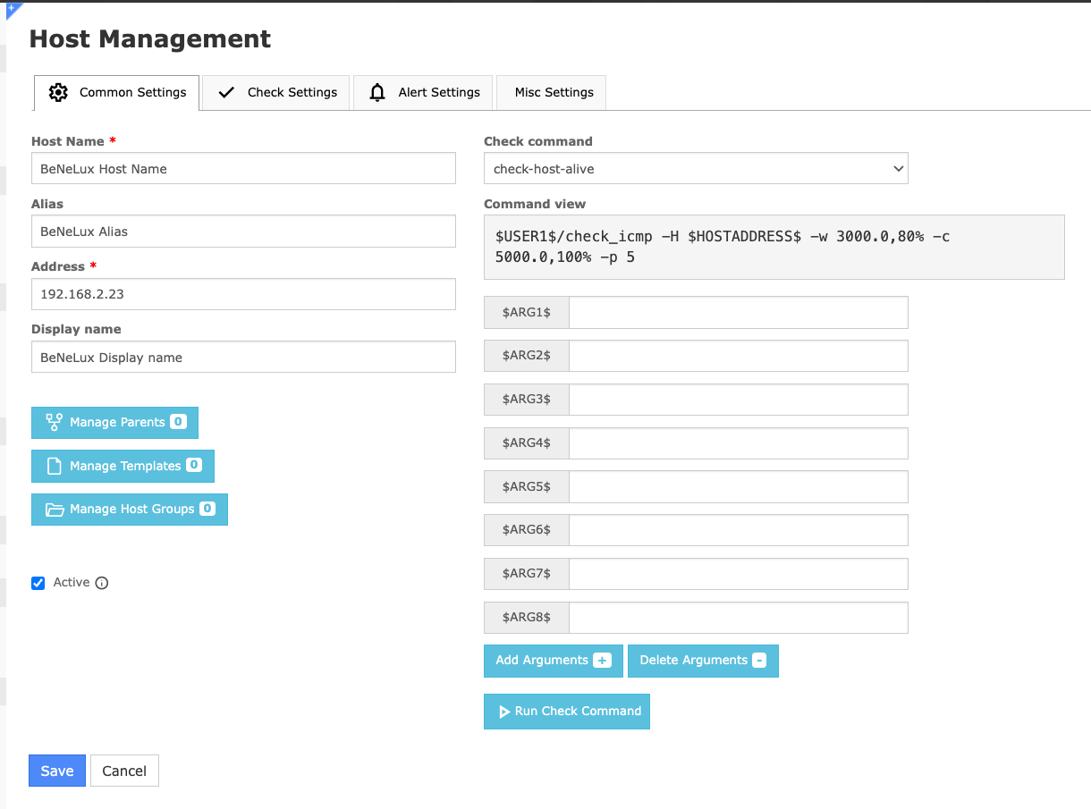
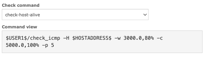
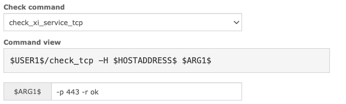

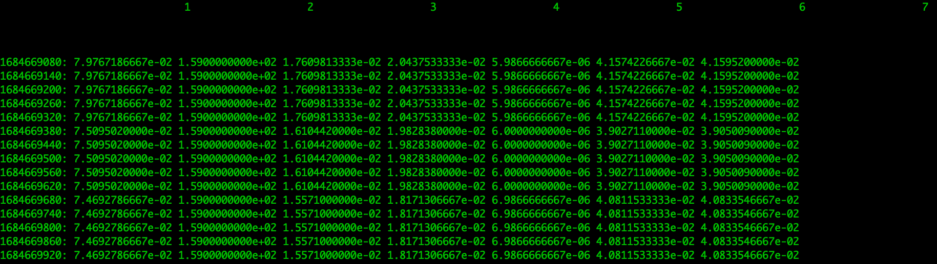
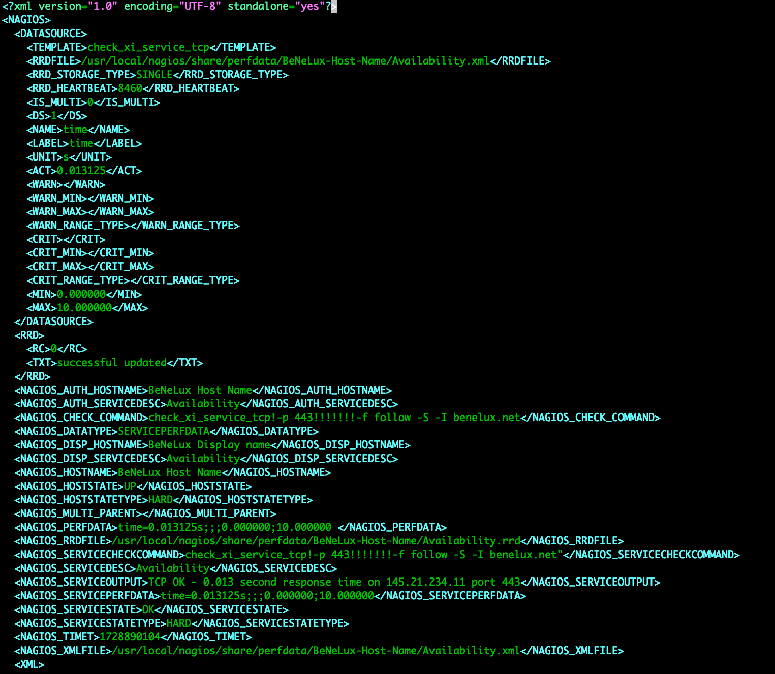
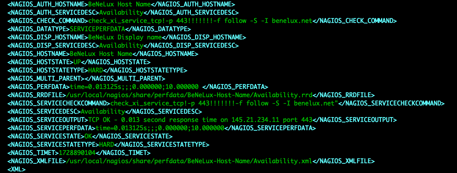
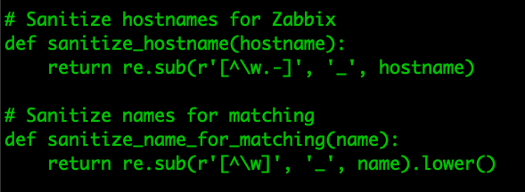
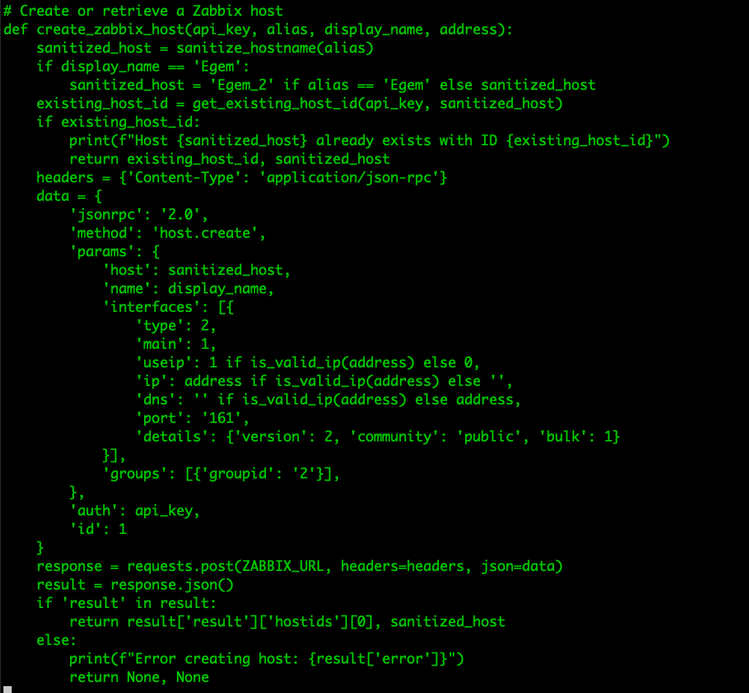
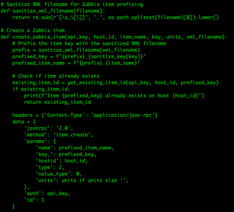
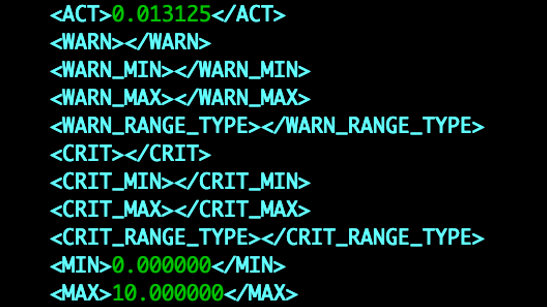
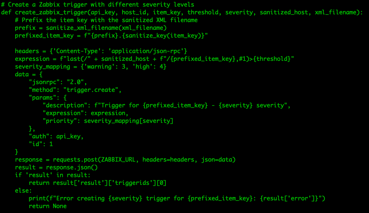
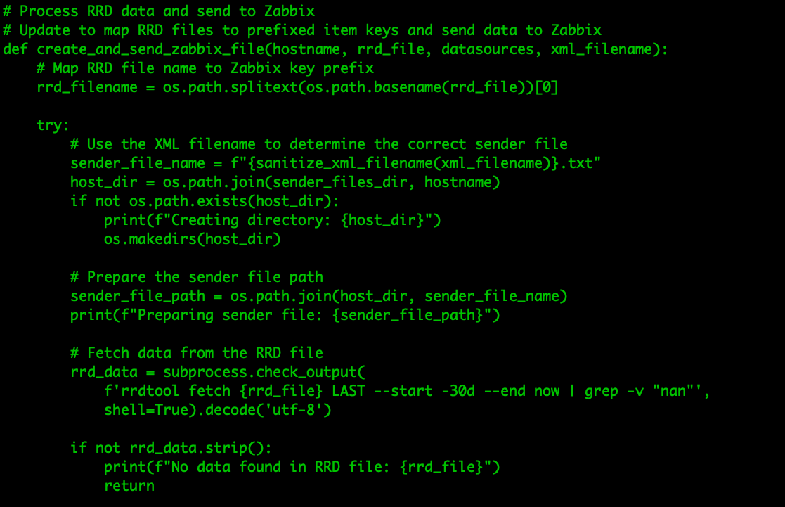
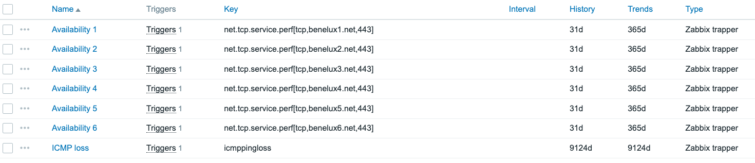
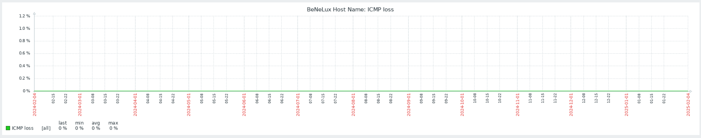

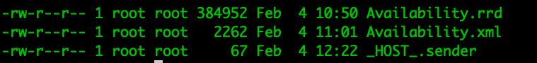
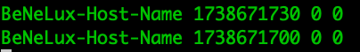
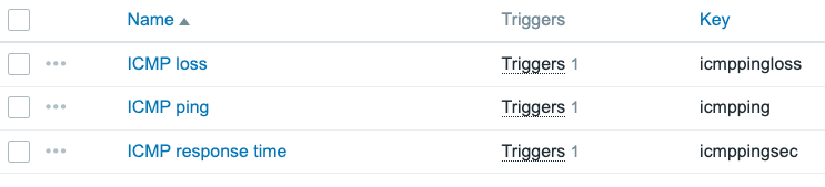
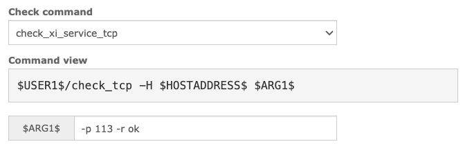
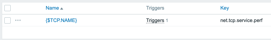
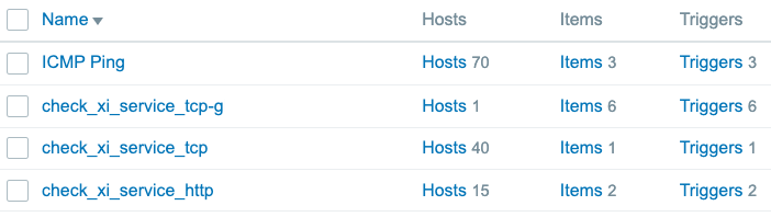
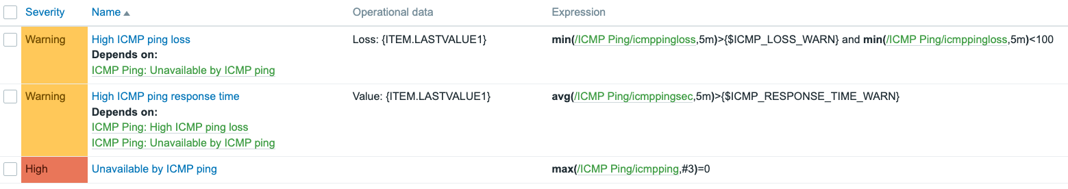


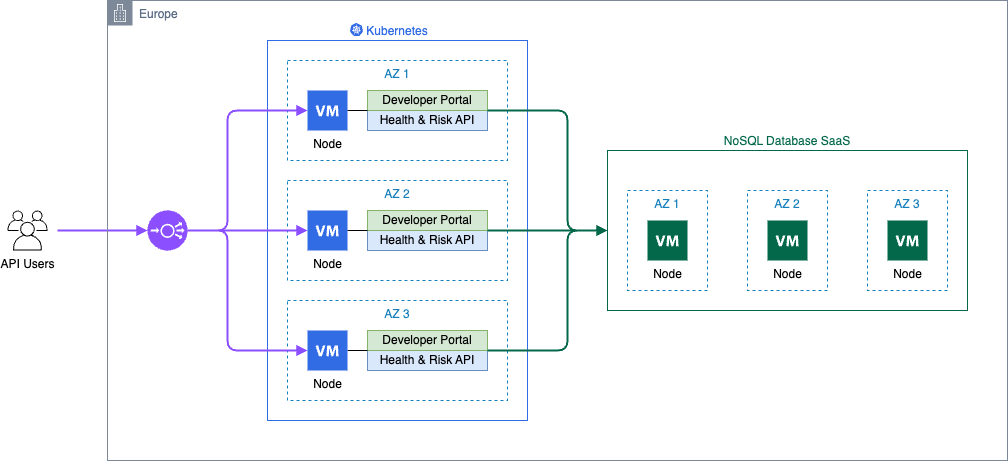


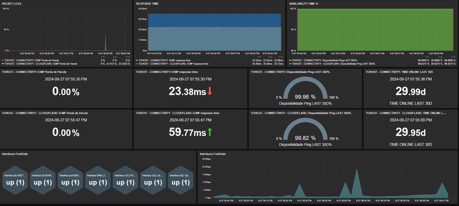

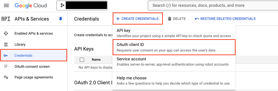


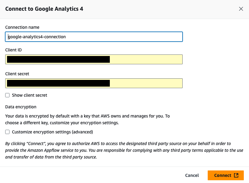
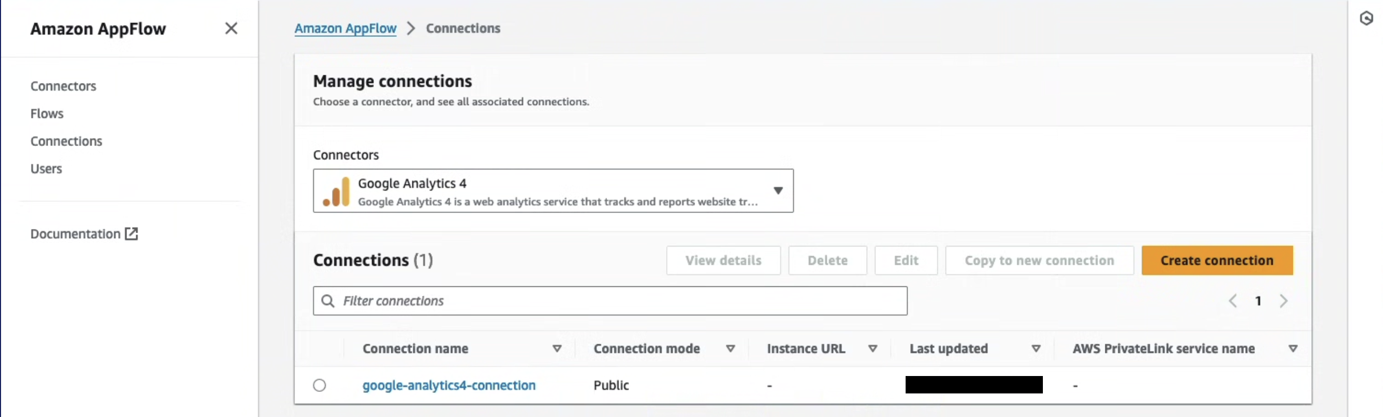
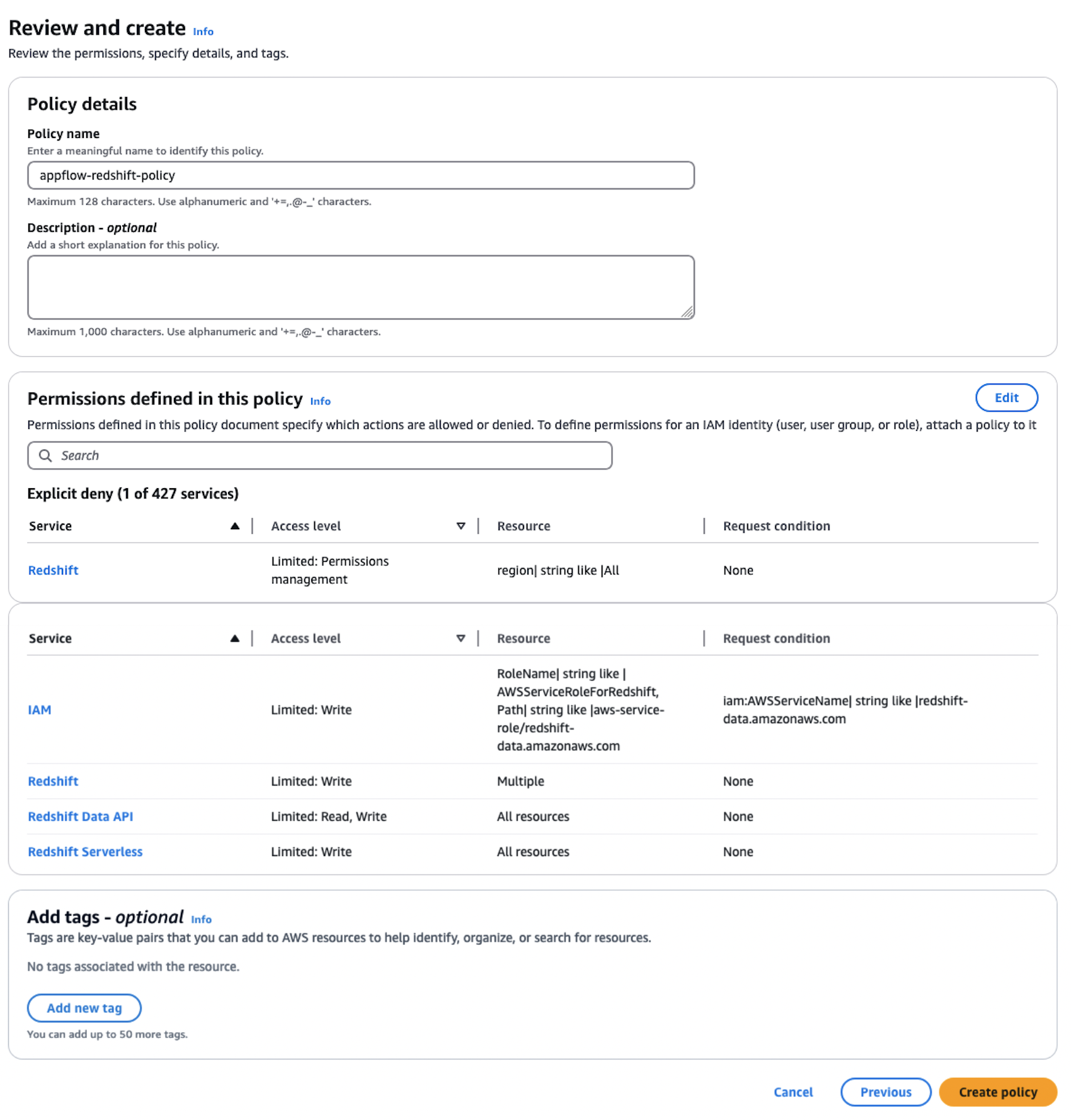


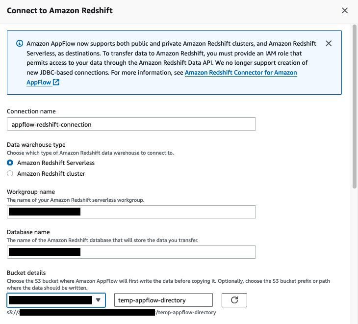
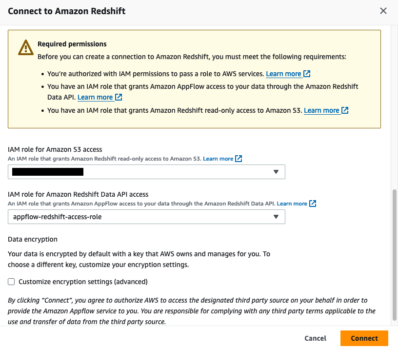


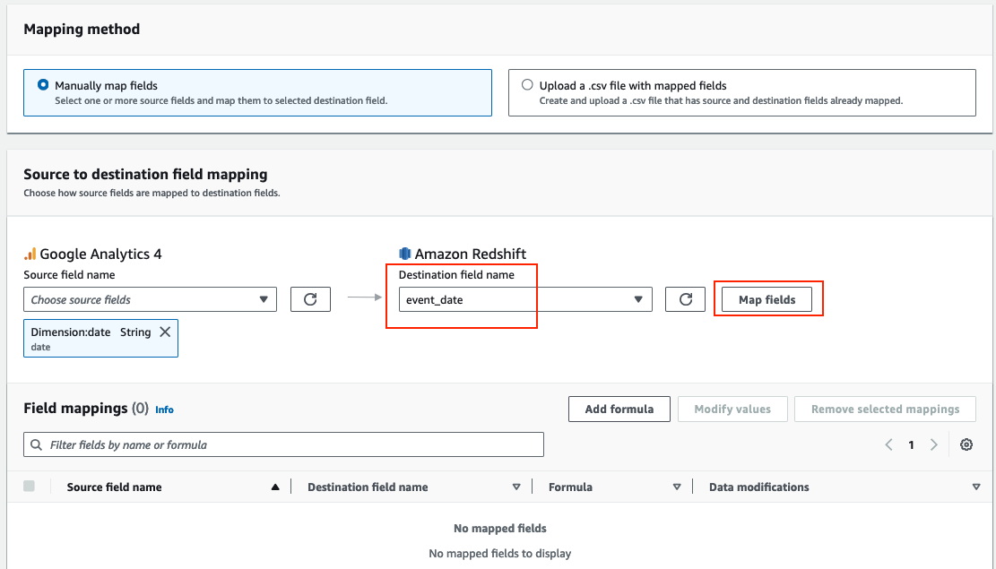


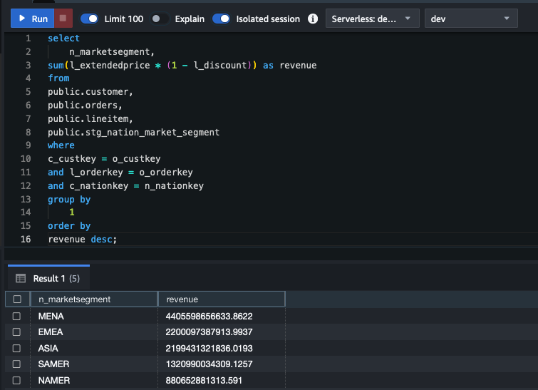
 Ritesh Kumar Sinha is an Analytics Specialist Solutions Architect based out of San Francisco. He has helped customers build scalable data warehousing and big data solutions for over 16 years. He loves to design and build efficient end-to-end solutions on AWS. In his spare time, he loves reading, walking, and doing yoga.
 Tahir Aziz is an Analytics Solution Architect at AWS. He has worked with building data warehouses and big data solutions for over 13 years. He loves to help customers design end-to-end analytics solutions on AWS. Outside of work, he enjoys traveling and cooking.
 Raza Hafeez is a Senior Product Manager at Amazon Redshift. He has over 13 years of professional experience building and optimizing enterprise data warehouses and is passionate about enabling customers to realize the power of their data. He specializes in migrating enterprise data warehouses to AWS Modern Data Architecture.
 Amit Ghodke is an Analytics Specialist Solutions Architect based out of Austin. He has worked with databases, data warehouses and analytical applications for the past 16 years. He loves to help customers implement analytical solutions at scale to derive maximum business value.


 Hang (Arthur) Zuo is a Senior Product Manager with Amazon OpenSearch Service. Arthur leads the core experience in the next-gen OpenSearch UI and data migration to Amazon OpenSearch Service. Arthur is passionate about cloud technologies and building data products that help users and businesses gain actionable insights and achieve operational excellence.
 Chris Helma is a Senior Engineer at Amazon Web Services based in Austin, Texas. He is currently developing tools and techniques to enable users to shift petabyte-scale data workloads into OpenSearch. He has extensive experience building highly-scalable technologies in diverse areas such as search, security analytics, cryptography, and developer productivity. He has functional domain expertise in distributed systems, AI/ML, cloud-native design, and optimizing DevOps workflows. In his free time, he loves to explore specialty coffee and run through the West Austin hills.
 Andre Kurait is a Software Development Engineer II at Amazon Web Services, based in Austin, Texas. He is currently working on Migration Assistant for Amazon OpenSearch Service. Prior to joining Amazon OpenSearch, Andre worked within Amazon Health Services. In his free time, Andre enjoys traveling, cooking, and playing in his church sport leagues. Andre holds Bachelor of the Science degrees from the University of Kansas in Computer Science and Mathematics.
 Prashant Agrawal is a Sr. Search Specialist Solutions Architect with Amazon OpenSearch Service. He works closely with customers to help them migrate their workloads to the cloud and helps existing customers fine-tune their clusters to achieve better performance and save on cost. Before joining AWS, he helped various customers use OpenSearch and Elasticsearch for their search and log analytics use cases. When not working, you can find him traveling and exploring new places. In short, he likes doing Eat → Travel → Repeat.


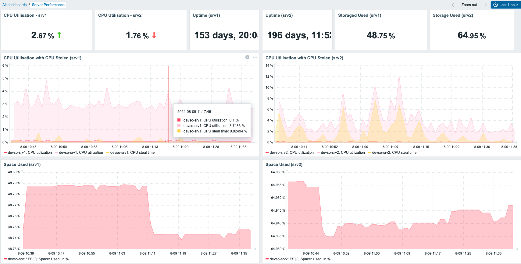
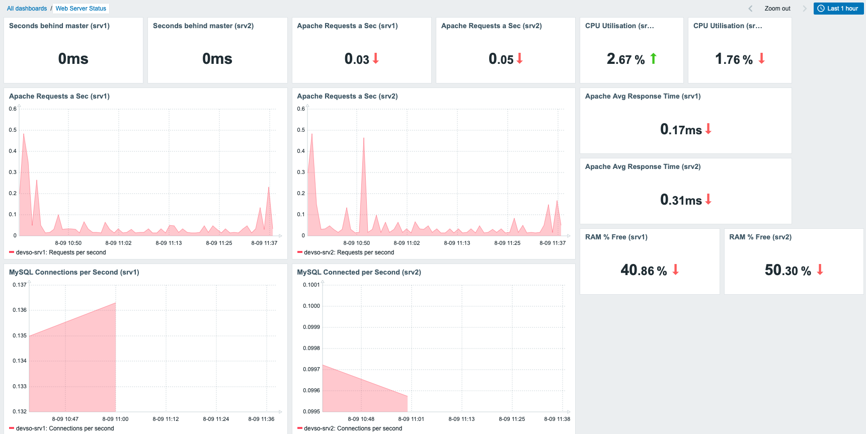


 Aswath Srinivasan is a Senior Search Engine Architect at Amazon Web Services currently based in Munich, Germany. With over 17 years of experience in various search technologies, Aswath currently focuses on OpenSearch. He is a search and open-source enthusiast and helps customers and the search community with their search problems.
 Jon Handler is a Senior Principal Solutions Architect at Amazon Web Services based in Palo Alto, CA. Jon works closely with OpenSearch and Amazon OpenSearch Service, providing help and guidance to a broad range of customers who have search and log analytics workloads that they want to move to the AWS Cloud. Prior to joining AWS, Jon’s career as a software developer included 4 years of coding a large-scale, ecommerce search engine. Jon holds a Bachelor of the Arts from the University of Pennsylvania, and a Master of Science and a PhD in Computer Science and Artificial Intelligence from Northwestern University.


 Sivaprasad Mahamkali is a Senior Streaming Data Engineer at AWS Professional Services. Siva leads customer engagements related to real-time streaming solutions, data lakes, analytics using opensource and AWS services. Siva enjoys listening to music and loves to spend time with his family.
 Dan Gibbar is a Senior Engagement Manager at AWS Professional Services. Dan leads healthcare and life science engagements collaborating with customers and partners to deliver outcomes. Dan enjoys the outdoors, attempting triathlons, music and spending time with family.
 Shrinath Parikh as a Senior Cloud Data Architect with AWS. He works with customers around the globe to assist them with their data analytics, data lake, data lake house, serverless, governance and NoSQL use cases. In Shrinath’s off time, he enjoys traveling, spending time with family and learning/building new tools using cutting edge technologies.
 Ramesh Daddala is a Associate Director at BMS. Ramesh leads enterprise data engineering engagements related to enterprise data lake services (EDLs) and collaborating with Data partners to deliver and support enterprise data engineering and ML capabilities. Ramesh enjoys the outdoors, traveling and loves to spend time with family.
 Jitendra Kumar Dash is a Senior Cloud Architect at BMS with expertise in hybrid cloud services, Infrastructure Engineering, DevOps, Data Engineering, and Data Analytics solutions. He is passionate about food, sports, and adventure.
 Pavan Kumar Bijja is a Senior Data Engineer at BMS. Pavan enables data engineering and analytical services to BMS Commercial domain using enterprise capabilities. Pavan leads enterprise metadata capabilities at BMS. Pavan loves to spend time with his family, playing Badminton and Cricket.
 Shovan Kanjilal is a Senior Data Lake Architect working with strategic accounts in AWS Professional Services. Shovan works with customers to design data and machine learning solutions on AWS.