Post Syndicated from Ramakant Joshi original https://aws.amazon.com/blogs/big-data/demystify-data-sharing-and-collaboration-patterns-on-aws-choosing-the-right-tool-for-the-job/
Data is the most significant asset of any organization. However, enterprises often encounter challenges with data silos, insufficient access controls, poor governance, and quality issues. Embracing data as a product is the key to address these challenges and foster a data-driven culture.
In this context, the adoption of data lakes and the data mesh framework emerges as a powerful approach. By decentralizing data ownership and distribution, enterprises can break down silos and enable seamless data sharing. Cataloging data, making the data searchable, implementing robust security and governance, and establishing effective data sharing processes are essential to this transformation. AWS offers services like AWS Data Exchange, AWS Glue, AWS Clean Rooms and Amazon DataZone to help organizations unlock the full potential of their data.
Personas
Let’s identify the various roles involved in the data sharing process.
First of all, there are data producers, which might include internal teams/systems, third-party producers, and partners. The data consumers include internal stakeholders/systems, external partners, and end-customers. At the core of this ecosystem lies the enterprise data platform. When considering enterprises, numerous personas come into play:
- Line of business users – These personas need to classify data, add business context, collaborate effectively with other lines of business, gain enhanced visibility into business key performance indicators (KPIs) for improved outcomes, and explore opportunities for monetizing data
- Partners – Partners should be able to share data, collaborate with other partners and customers.
- Data scientists and business analysts – These personas should be able to access the data, analyze it and generate actionable business insights
- Data engineers – Data engineers are tasked with building the proper data pipeline and cataloging the data that meets the diverse needs of stakeholders, including business analysts, data scientists, partners, and line of business users
- Data security and governance officers – Data security involves making sure producers and consumers have appropriate access to the data, implementing right access permissions, and maintaining compliance with industry regulations, particularly in highly regulated sectors like healthcare, life sciences, and financial services. This persona is also responsible for enhancing data governance by tracking lineage, and establishing data mesh policies
Choosing the right tool for the job
Now that you have identified the various personas, it’s important to select the appropriate tools for each role:
- Starting with the producers, if your data source includes a software as a service (SaaS) platform, AWS Glue offers options to automate data flows between software service providers and AWS services.
- For producers seeking collaboration with partners, AWS Clean Rooms facilitates secure collaboration and analysis of collective datasets without the need to share or duplicate underlying data.
- When dealing with third-party data sources, AWS Data Exchange simplifies the discovery, subscription, and utilization of third-party data from a diverse range of producers or providers. As a producer, you can also monetize your data through the subscription model using AWS Data Exchange.
- Within your organization, you can democratize data with governance, using Amazon DataZone, which offers built-in governance features.
- For SaaS consumers, AWS Glue supports bidirectional transfer and serves both as a producer and consumer tool for various SaaS providers.
Let’s briefly describe the capabilities of the AWS services we referred above:
AWS Glue is a fully managed, serverless, and scalable extract, transform, and load (ETL) service that simplifies the process of discovering, preparing, and loading data for analytics. It provides data catalog, automated crawlers, and visual job creation to streamline data integration across various data sources and targets.
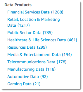
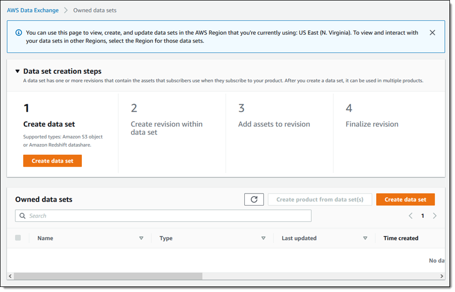
AWS Data Exchange enables you to find, subscribe to, and use third-party datasets in the AWS Cloud. It also provides a platform through which a data producer can make their data available for consumption for subscribers. It is a data marketplace featuring over 300 providers offering thousands of datasets accessible through files, Amazon Redshift tables, and APIs. This service supports consolidated billing and subscription management, offering you the flexibility to explore 1,000 free datasets and samples. You don’t need to set up a separate billing mechanism or payment method specifically for AWS Data Exchange subscriptions.
AWS Clean Rooms is designed to assist companies and their partners in securely analyzing and collaborating on collective datasets without revealing or sharing underlying data. You can swiftly create a secure data clean room, fostering collaboration with other entities on the AWS Cloud to derive unique insights for initiatives such as advertising campaigns or research and development. This service protects underlying data through a comprehensive set of privacy-enhancing controls and flexible analysis rules tailored to specific business needs.
Amazon DataZone is a data management service that makes it fast and straightforward to catalog, discover, share, and govern data stored across AWS, on-premises, and third-party sources. With Amazon DataZone, administrators and data stewards who oversee an organization’s data assets can manage and govern access to data using fine-grained controls. These controls are designed to grant access with the right level of privileges and context. Amazon DataZone makes it straightforward for engineers, data scientists, product managers, analysts, and business users to access data throughout an organization so they can discover, use, and collaborate to derive data-driven insights.
Use cases
Let’s review some example use cases to understand how these diverse services can be effectively applied within a business context to achieve the desired outcomes. In this particular scenario, we focus on a company named AnyHealth, which operates in the healthcare and life sciences sector. This company encompasses multiple lines of businesses, specializing in the sale of various scientific equipment. Three key requirements have been identified:
- Sales and customer visibility by line of business – AnyHealth wants to gain insights into the sales performance and customer demands specific to each line of business. This necessitates a comprehensive view of sales activities and customer requirements tailored to individual lines of business.
- Cross-organization supply chain and inventory visibility – The company faces challenges related to supply chain and inventory management, especially in global crisis situations like a pandemic. They want to address instances where inventory items are idle in one line of business while there is demand for the same items in another. To overcome this, they want to establish cross-organizational visibility of supply chain and inventory data, breaking down silos and achieving prompt responses to business demands.
- Cross-sell and up-sell opportunities – AnyHealth intends to boost sales by implementing cross-selling and up-selling strategies. To achieve this, they plan to use machine learning (ML) models to extract insights from data. These insights will then be provided to sales representatives and resellers, enabling them to identify and capitalize on opportunities effectively.
In the following sections, we discuss how to address each requirement in more detail and the AWS services that best fit each solution.
Sales and customer visibility by line of business
The first requirement involves obtaining visibility into sales and customer demand by line of business. The key consumers of this data include line of business leaders, business analysts, and various other business stakeholders.
The initial step is to ingest sales and order data into the platform. Currently, this data is centralized in the ERP system, specifically SAP. The objective is to regularly retrieve this data and capture any changes that occur. The data engineers are instrumental in building this pipeline. Given that we are dealing with a SaaS integration, AWS Glue is the logical choice for seamless data ingestion.
Next, we focus on building the enterprise data platform where the accumulated data will be hosted. This platform will incorporate robust cataloging, making sure the data is easily searchable, and will enforce the necessary security and governance measures for selective sharing among business stakeholders, data engineers, analysts, security and governance officers. In this context, Amazon DataZone is the optimal choice for managing the enterprise data platform.
As stated earlier, the first step involves data ingestion. Data is ingested from a third-party vendor SaaS solution (SAP), and the data engineer uses AWS Glue. Utilizing the SAP data connector, the data engineer establishes a connection with the SAP environment, running scheduled jobs.
The data lands in Amazon Simple Storage Service (Amazon S3). Additional AWS Glue jobs are created to transform and curate the data. The curated data is placed in a designated bucket and AWS Glue crawlers are run to catalog the data. This cataloged data is then managed through Amazon DataZone.
In Amazon DataZone, the data security officer creates the corporate domain. She/he creates producer projects and enables access to data engineers, and business analysts. Data engineers ensure sales and customer data is available from the source into the Amazon DataZone project. Business analysts enhance the data with business metadata/glossaries and publish the same as data assets or data products. The data security officer sets permissions in Amazon DataZone to allow users to access the data portal. Users can search for assets in the Amazon DataZone catalog, view the metadata assigned to them, and access the assets.
Amazon Athena is used to query, and explore the data. Amazon QuickSight is used to read from Amazon Athena and generate reports that is consumed by the line of business users and other stakeholders.
The following diagram illustrates the solution architecture using AWS services.

Cross-organization supply chain and inventory visibility
For the second requirement, the objective is to achieve visibility of supply chain and inventory across the organization. The key stakeholders remain line of business users. They would like to get a cross-organization visibility of supply chain and inventory data. The aim is to ingest supply chain and inventory information in a scheduled manner from the ERP system (SAP), and also capture any changes in the supply chain and inventory data. The persona involved in setting up the data ingestion pipeline is a data engineer. Given that we are extracting data from SAP, AWS Glue is the suitable choice for this requirement.
The next step involves obtaining economic indicators and weather information from third-party sources. AnyHealth, with its diverse lines of business, including one that manufactures medical equipment such as inhalers for asthma treatment, recognizes the significance of collecting weather information, particularly data about pollen, because it directly impacts the patient population. Additionally, socioeconomic conditions play a crucial role in government-assisted programs related to out-of-hospital care. To incorporate this third-party data, AWS Data Exchange is the logical choice.
Finally, all the accumulated data needs to be hosted on the enterprise data platform, with cataloging, and robust security and governance measures. In this context, Amazon DataZone is the preferred solution.
The pipeline begins with the ingestion of data from SAP, facilitated by AWS Glue. The data lands in Amazon S3, where AWS Glue jobs are used to curate the data, generate curated tables, and then AWS Glue crawlers are used to catalog the data.
AWS Data Exchange serves as the platform for collecting economic trends and weather information. The business analyst leverages AWS Data Exchange to retrieve data from various sources. In the AWS Data Exchange marketplace, they identify the data set, subscribe to the data, and subsequently consume it. Any changes in the source data invokes events, which updates the data object in the Amazon S3 bucket.
Amazon DataZone is used to manage and govern the datalake. Similar to the first use case, the data security officer creates a producer project. The data owner from LoB creates supply chain and inventory data assets in the producer project and publishes the same. From the consumer perspective, the data security officer also creates a consumer project, which allows the sales and marketing teams from different LoBs to search for the supply chain and inventory data published by the producer. Consumers request access to the published supply chain and inventory data, and the producer grants the necessary access. Amazon Athena is used to query, and explore the data. Amazon QuickSight is used to read from Amazon Athena and generate reports.
The following diagram illustrates this architecture.

Cross-sell and up-sell opportunities
The third requirement involves identifying cross-sell and up-sell opportunities. The key business consumers in this context are the sales representatives and resellers. AnyHealth operates globally, selling products in Europe, America, and Asia. Direct business transactions with consumers occur in America and Europe, and resellers facilitate sales in Asia, where AnyHealth lacks a direct relationship with the consumers.
The enterprise data platform is used to host and analyze the sales data and identify the customer demand. This data platform is managed by Amazon Data Zone. Cross-sell and up-sell opportunities, derived through ML models, are integrated into the customer relationship management (CRM) system, which in this case is Salesforce. Sales representatives access this data from Salesforce to engage with the market and collaborate with customers. AWS Glue is used for this integration.
Typically, resellers don’t provide their partners direct access to their customer data. Although AnyHealth doesn’t have direct access, understanding customer personas and profile information is essential to equip resellers with right offers to cross-sell and up-sell products. AWS Clean Rooms enables collaboration on collective datasets with stringent security controls, enabling insights without sharing the underlying data.
By addressing these requirements, AnyHealth can effectively identify and capitalize on cross-sell and up-sell opportunities, tailoring their approach based on the distinct dynamics of direct and reseller-based business models across various regions.
The initial step in the architecture involves a pipeline where SAP data is ingested into Amazon S3 and curated using AWS Glue job. The curated data is cataloged, governed and managed using Amazon DataZone.
In this scenario, where sales and customer information are acquired, data scientists build ML models to identify cross-sell and upsell opportunities. Using Amazon DataZone, these opportunities are shared with line of business users, providing transparency regarding the opportunities presented to sales reps and resellers. The cross-sell and upsell insights are pushed to Salesforce through AWS Glue, with an event-driven workflow for timely communication to sales reps. However, for resellers, a different pipeline is needed as AnyHealth doesn’t have direct access to the customer sales data. AnyHealth uses AWS Clean Rooms for this purpose.
With AWS Clean Rooms, the collaboration is started by AnyHealth (the collaboration initiator) who invites resellers to join. Resellers participate in the collaboration, and share the customer profile and segment information, while maintaining privacy by excluding customer names and contact details. AnyHealth uses the customer profile information and order trends to identify cross-sell and upsell opportunities. These opportunities are shared with the reseller to pursue further and position products in the market.
The following diagram illustrates this architecture.

Final architecture
Let’s now examine the complete architecture which covers all three use cases. In this architecture, purpose-built services like AWS Data Exchange, AWS Glue, AWS Clean Rooms and Amazon DataZone, have been used. The seamless integration of these services works cohesively to achieve end-to-end business objectives.
The following diagram illustrates this architecture.

To strengthen the security posture of your cloud infrastructure, we recommend using AWS Identity and Access Management (IAM), which allows you to manage access to AWS resources by creating users, groups, and roles with specific permissions. Additionally, you can use AWS Key Management Service (AWS KMS), which enables you to create, manage, and control encryption keys used to protect your data, so only authorized entities can access sensitive information. To provide an audit trail for compliance, you can use AWS CloudTrail, which records API calls made within your AWS account.
Conclusion
In this post, we discussed how to choose right tool for building an enterprise data platform and enabling data sharing, collaboration and access within your organization and with third-party providers. We addressed three business use cases using AWS Glue, AWS Data Exchange, AWS Clean Rooms, and Amazon DataZone through three different use cases.
To learn more about these services, check out the AWS Blogs for Amazon DataZone, AWS Glue, AWS Clean Rooms, and AWS Data Exchange.
About the authors
 Ramakant Joshi is an AWS Solutions Architect, specializing in the analytics and serverless domain. He has a background in software development and hybrid architectures, and is passionate about helping customers modernize their cloud architecture.
 Debaprasun Chakraborty is an AWS Solutions Architect, specializing in the analytics domain. He has around 20 years of software development and architecture experience. He is passionate about helping customers in cloud adoption, migration and strategy.


 Saurabh Bhutyani is a Principal Analytics Specialist Solutions Architect at AWS. He is passionate about new technologies. He joined AWS in 2019 and works with customers to provide architectural guidance for running generative AI use cases, scalable analytics solutions and data mesh architectures using AWS services like Amazon Bedrock, Amazon SageMaker, Amazon EMR, Amazon Athena, AWS Glue, AWS Lake Formation, and Amazon DataZone.
 Ankith Ede is a Data & Machine Learning Engineer at Amazon Web Services, based in New York City. He has years of experience building Machine Learning, Artificial Intelligence, and Analytics based solutions for large enterprise clients across various industries. He is passionate about helping customers build scalable and secure cloud based solutions at the cutting edge of technology innovation.
 Chandra Krishnan is a Solutions Engineer at Onehouse, based in New York City. He works on helping Onehouse customers build business value from their data lakehouse deployments and enjoys solving exciting challenges on behalf of his customers. Prior to Onehouse, Chandra worked at AWS as a Data and ML Engineer, helping large enterprise clients build cutting edge systems to drive innovation in their organizations.


 Sandipan Bhaumik is a Senior Analytics Specialist Solutions Architect based in London, UK. He helps customers modernize their traditional data platforms using the modern data architecture in the cloud to perform analytics at scale.
 Sain Das is a Senior Product Manager on the Amazon Redshift team and leads Amazon Redshift GTM for partner programs, including the Powered by Amazon Redshift and Redshift Ready programs.


 Tony Stricker is a Principal Technologist on the Data Strategy team at AWS, where he helps senior executives adopt a data-driven mindset and align their people/process/technology in ways that foster innovation and drive towards specific, tangible business outcomes. He has a background as a data warehouse architect and data scientist and has delivered solutions in to production across multiple industries including oil and gas, financial services, public sector, and manufacturing. In his spare time, Tony likes to hang out with his dog and cat, work on home improvement projects, and restore vintage Airstream campers.

 Venkata Sistla is a Cloud Architect – Data & Analytics at AWS. He specializes in building data processing capabilities and helping customers remove constraints that prevent them from leveraging their data to develop business insights.
 Santosh Chiplunkar is a Principal Resident Architect at AWS. He has over 20 years of experience helping customers solve their data challenges. He helps customers develop their data and analytics strategy and provides them with guidance on how to make it a reality.

 Jon Roberts is a Sr. Analytics Specialist based out of Nashville, specializing in Amazon Redshift. He has over 27 years of experience working in relational databases. In his spare time, he runs.


 You can also automate the preceding COPY commands using tasks, which can be scheduled to run at a set frequency for automatic copy of CDC data from Snowflake to Amazon S3.
 Now the tasks will run every 5 minutes and look for new data in the stream tables to offload to Amazon S3.As soon as data is migrated from Snowflake to Amazon S3, Redshift Auto Loader automatically infers the schema and instantly creates corresponding tables in Amazon Redshift. Then, by default, it starts loading data from Amazon S3 to Amazon Redshift every 5 minutes. You can also