Post Syndicated from Matt Bullock original https://blog.cloudflare.com/new-standards
As the Internet grows, so do the demands for speed and security. At Cloudflare, we’ve spent the last 14 years simplifying the adoption of the latest web technologies, ensuring that our users stay ahead without the complexity. From being the first to offer free SSL certificates through Universal SSL to quickly supporting innovations like TLS 1.3, IPv6, and HTTP/3, we’ve consistently made it easy for everyone to harness cutting-edge advancements.
One of the most exciting recent developments in web performance is Zstandard (zstd) — a new compression algorithm that we have found compresses data 42% faster than Brotli while maintaining almost the same compression levels. Not only that, but Zstandard reduces file sizes by 11.3% compared to GZIP, all while maintaining comparable speeds. As compression speed and efficiency directly impact latency, this is a game changer for improving user experiences across the web.
We’re also re-starting the rollout of Encrypted Client Hello (ECH), a new proposed standard that prevents networks from snooping on which websites a user is visiting. Encrypted Client Hello (ECH) is a successor to ESNI and masks the Server Name Indication (SNI) that is used to negotiate a TLS handshake. This means that whenever a user visits a website on Cloudflare that has ECH enabled, no one except for the user, Cloudflare, and the website owner will be able to determine which website was visited. Cloudflare is a big proponent of privacy for everyone and is excited about the prospects of bringing this technology to life.
In this post, we also further explore our work measuring the impact of HTTP/3 prioritization, and the development of Bottleneck Bandwidth and Round-trip propagation time (BBR) congestion control to further optimize network performance.
Introducing Zstandard compression
Zstandard, an advanced compression algorithm, was developed by Yann Collet at Facebook and open sourced in August 2016 to manage large-scale data processing. It has gained popularity in recent years due to its impressive compression ratios and speed. The protocol was included in Chromium-based browsers and Firefox in March 2024 as a supported compression algorithm.
Today, we are excited to announce that Zstandard compression between Cloudflare and browsers is now available to everyone.
Our testing shows that Zstandard compresses data up to 42% faster than Brotli while achieving nearly equivalent data compression. Additionally, Zstandard outperforms GZIP by approximately 11.3% in compression efficiency, all while maintaining similar compression speeds. This means Zstandard can compress files to the same size as Brotli but in nearly half the time, speeding up your website without sacrificing performance.
This is exciting because compression speed and file size directly impacts latency. When a browser requests a resource from the origin server, the server needs time to compress the data before it’s sent over the network. A faster compression algorithm, like Zstandard, reduces this initial processing time. By also reducing the size of files transmitted over the Internet, better compression means downloads take less time to complete, websites load quicker, and users ultimately get a better experience.

Why is compression so important?
Website performance is crucial to the success of online businesses. Study after study has shown that an increased load time directly affects sales. In highly competitive markets, the performance of a website is crucial for success. Just like a physical shop situated in a remote area faces challenges in attracting customers, a slow website encounters similar difficulties in attracting traffic.
Think about buying a piece of flat pack furniture such as a bookshelf. Instead of receiving the bookshelf fully assembled, which would be expensive and cumbersome to transport, you receive it in a compact, flat box with all the components neatly organized, ready for assembly. The parts are carefully arranged to take up the least amount of space, making the package much smaller and easier to handle. When you get the item, you simply follow the instructions to assemble it to its proper state.
This is similar to how data compression works. The data is “disassembled” and packed tightly to reduce its size before being transmitted. Once it reaches its destination, it’s “reassembled” to its original form. This compression process reduces the amount of data that needs to be sent, saving bandwidth, reducing costs, and speeding up the transfer, just like how flat pack furniture reduces shipping costs and simplifies delivery logistics.
However, with compression, there is a tradeoff: time to compress versus the overall compression ratio. A compression ratio is a measure of how much a file’s size is reduced during compression. For example, a 10:1 compression ratio means that the compressed file is one-tenth the size of the original. Just like assembling flat-pack furniture takes time and effort, achieving higher compression ratios often requires more processing time. While a higher compression ratio significantly reduces file size — making data transmission faster and more efficient — it may take longer to compress and decompress the data. Conversely, quicker compression methods might produce larger files, leading to faster processing but at the cost of greater bandwidth usage. Balancing these factors is key to optimizing performance in data transmission.
W3 Technologies reports that as of September 12, 2024, 88.6% of websites rely on compression to optimize speed and reduce bandwidth usage. GZIP, introduced in 1996, remains the default algorithm for many, used by 57.0% of sites due to its reasonable compression ratios and fast compression speeds. Brotli, released by Google in 2016, delivers better compression ratios, leading to smaller file sizes, especially for static assets like JavaScript and CSS, and is used by 45.5% of websites. However, this also means that 11.4% of websites still operate without any compression, missing out on crucial performance improvements.
As the Internet and its supporting infrastructure have evolved, so have user demands for faster, more efficient performance. This growing need for higher efficiency without compromising speed is where Zstandard comes into play.
Enter Zstandard
Zstandard offers higher compression ratios comparable to GZIP, but with significantly faster compression and decompression speeds than Brotli. This makes it ideal for real-time applications that require both speed and relatively high compression ratios.
To understand Zstandard’s advantages, it’s helpful to know about Zlib. Zlib was developed in the mid-1990s based on the DEFLATE compression algorithm, which combines LZ77 and Huffman coding to reduce file sizes. While Zlib has been a compression standard since the mid-1990s and is used in Cloudflare’s open-source GZIP implementation, its design is limited by a 32 KB sliding window — a constraint from the memory limitations of that era. This makes Zlib less efficient on modern hardware, which can access far more memory.
Zstandard enhances Zlib by leveraging modern innovations and hardware capabilities. Unlike Zlib’s fixed 32 KB window, Zstandard has no strict memory constraints and can theoretically address terabytes of memory. However, in practice, it typically uses much less, around 1 MB at lower compression levels. This flexibility allows Zstandard to buffer large amounts of data, enabling it to identify and compress repeating patterns more effectively. Zstandard also employs repcode modeling to efficiently compress structured data with repetitive sequences, further reducing file sizes and enhancing its suitability for modern compression needs.
Zstandard is optimized for modern CPUs, which can execute multiple tasks simultaneously using multiple Arithmetic Logic Units (ALUs) that are used to perform mathematical tasks. Zstandard achieves this by processing data in parallel streams, dividing it into multiple parts that are processed concurrently. The Huffman decoder, Huff0, can decode multiple symbols in parallel on a single CPU core, and when combined with multi-threading, this leads to substantial speed improvements during both compression and decompression.
Zstandard’s branchless design is a crucial innovation that enhances CPU efficiency, especially in modern processors. To understand its significance, consider how CPUs execute instructions.
Modern CPUs use pipelining, where different stages of an instruction are processed simultaneously—like a production line—keeping all parts of the processor busy. However, when CPUs encounter a branch, such as an ‘if-else’ decision, they must make a branch prediction to guess the next step. If the prediction is wrong, the pipeline must be cleared and restarted, causing slowdowns.
Zstandard avoids this issue by eliminating conditional branching. Without relying on branch predictions, it ensures the CPU can execute instructions continuously, keeping the pipeline full and avoiding performance bottlenecks.
A key feature of Zstandard is its use of Finite State Entropy (FSE), an advanced compression method that encodes data more efficiently based on probability. FSE, built on the Asymmetric Numeral System (ANS), allows Zstandard to use fractional bits for encoding, unlike traditional Huffman coding, which only uses whole bits. This allows heavily repeated data to be compressed more tightly without sacrificing efficiency.
Zstandard findings
In the third quarter of 2024, we conducted extensive tests on our new Zstandard compression module, focusing on a 24-hour period where we switched the default compression algorithm from Brotli to Zstandard across our Free plan traffic. This experiment spanned billions of requests, covering a wide range of file types and sizes, including HTML, CSS, and JavaScript. The results were very promising, with significant improvements in both compression speed and file size reduction, leading to faster load times and more efficient bandwidth usage.
Compression ratios
In terms of compression efficiency, Zstandard delivers impressive results. Below are the average compression ratios we observed during our testing.
|
Compression Algorithm |
Average Compression Ratio |
|
GZIP |
2.56 |
|
Zstandard |
2.86 |
|
Brotli |
3.08 |
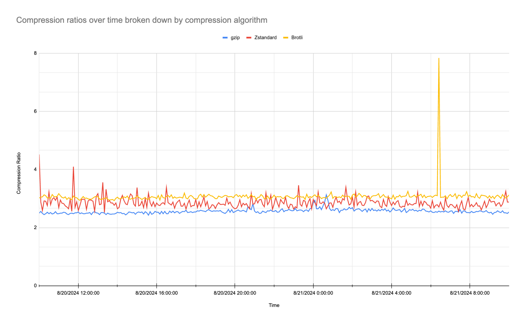
As the table shows, Zstandard achieves an average compression ratio of 2.86:1, which is notably higher than gzip’s 2.56:1 and close to Brotli’s 3.08:1. While Brotli slightly edges out Zstandard in terms of pure compression ratio, what is particularly exciting is that we are only using Zstandard’s default compression level of 3 (out of 22) on our traffic. In the fourth quarter of 2024, we plan to experiment with higher compression levels and multithreading capabilities to further enhance Zstandard’s performance and optimize results even more.
Compression speeds
What truly sets Zstandard apart is its speed. Below are the average times to compress data from our traffic-based tests measured in milliseconds:
|
Compression Algorithm |
Average Time to Compress (ms) |
|
GZIP |
0.872 |
|
Zstandard |
0.848 |
|
Brotli |
1.544 |
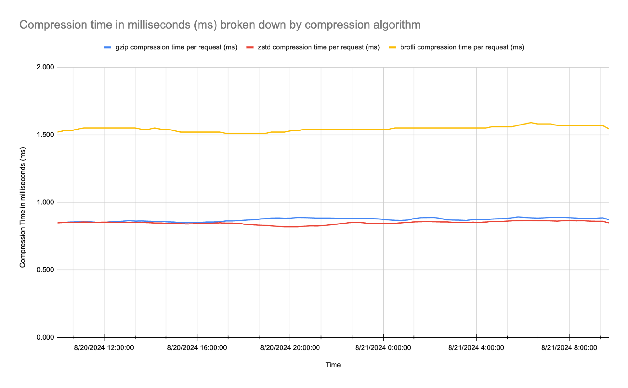
Zstandard not only compresses data efficiently, but it also does so 42% faster than Brotli, with an average compression time of 0.848 ms compared to Brotli’s 1.544 ms. It even outperforms gzip, which compresses at 0.872 ms on average.
From our results, we have found Zstandard strikes an excellent balance between achieving a high compression ratio and maintaining fast compression speed, making it particularly well-suited for dynamic content such as HTML and non-cacheable sensitive data. Zstandard can compress these responses from the origin quickly and efficiently, saving time compared to Brotli while providing better compression ratios than GZIP.
Implementing Zstandard at Cloudflare
To implement Zstandard compression at Cloudflare, we needed to build it into our Nginx-based service which already handles GZIP and Brotli compression. Nginx is modular by design, with each module performing a specific function, such as compressing a response. Our custom Nginx module leverages Nginx’s function ‘hooks’ — specifically, the header filter and body filter — to implement Zstandard compression.
Header filter
The header filter allows us to access and modify response headers. For example, Cloudflare only compresses responses above a certain size (50 bytes for Zstandard), which is enforced with this code:
if (r->headers_out.content_length_n != -1 &&
    r->headers_out.content_length_n < conf->min_length) {
    return ngx_http_next_header_filter(r);
}
Here, we check the “Content-Length” header. If the content length is less than our minimum threshold, we skip compression and let Nginx execute the next module.
We also need to ensure the content is not already compressed by checking the “Content-Encoding” header:
if (r->headers_out.content_encoding &&
    r->headers_out.content_encoding->value.len) {
    return ngx_http_next_header_filter(r);
}
If the content is already compressed, the module is bypassed, and Nginx proceeds to the next header filter.
Body filter
The body filter hook is where the actual processing of the response body occurs. In our case, this involves compressing the data with the Zstandard encoder and streaming the compressed data back to the client. Since responses can be very large, it’s not feasible to buffer the entire response in memory, so we manage internal memory buffers carefully to avoid running out of memory.
The Zstandard library is well-suited for streaming compression and provides the ZSTD_compressStream2 function:
ZSTDLIB_API size_t ZSTD_compressStream2(ZSTD_CCtx* cctx,
                                        ZSTD_outBuffer* output,
                                        ZSTD_inBuffer* input,
                                        ZSTD_EndDirective endOp);
This function can be called repeatedly with chunks of input data to be compressed. It accepts input and output buffers and an “operation” parameter (ZSTD_EndDirective endOp) that controls whether to continue feeding data, flush the data, or finalize the compression process.
Nginx uses a “flush” flag on memory buffers to indicate when data can be sent. Our module uses this flag to set the appropriate Zstandard operation:
switch (zstd_operation) {
    case ZSTD_e_continue: {
        if (flush) {
            zstd_operation = ZSTD_e_flush;
        }
    }
}
This logic allows us to switch from the “ZSTD_e_continue” operation, which feeds more input data into the encoder, to “ZSTD_e_flush”, which extracts compressed data from the encoder.
Compression cycle
The compression module operates in the following cycle:
-
Receive uncompressed data.
-
Locate an internal buffer to store compressed data.
-
Compress the data with Zstandard.
-
Send the compressed data back to the client.
Once a buffer is filled with compressed data, it’s passed to the next Nginx module and eventually sent to the client. When the buffer is no longer in use, it can be recycled, avoiding unnecessary memory allocation. This process is managed as follows:
if (free) {
    // A free buffer is available, so use it
    buffer = free;
} else if (buffers_used < maximum_buffers) {
    // No free buffers, but we're under the limit, so allocate a new one
    buffer = create_buf();
} else {
    // No free buffers and can't allocate more
    err = no_memory;
}
Handling backpressure
If no buffers are available, it can lead to backpressure — a situation where the Zstandard module generates compressed data faster than the client can receive it. This causes data to become “stuck” inside Nginx, halting further compression due to memory constraints. In such cases, we stop compression and send an empty buffer to the next Nginx module, allowing Nginx to attempt to send the data to the client again. When successful, this frees up memory buffers that our module can reuse, enabling continued streaming of the compressed response without buffering the entire response in memory.
What’s next? Compression dictionaries
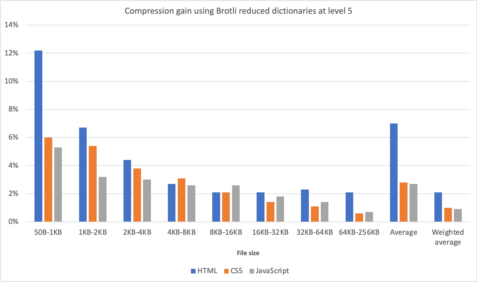
The future of Internet compression lies in the use of compression dictionaries. Both Brotli and Zstandard support dictionaries, offering up to 90% improvement on compression levels compared to using static dictionaries.
Compression dictionaries store common patterns or sequences of data, allowing algorithms to compress information more efficiently by referencing these patterns rather than repeating them. This concept is akin to how an iPhone’s predictive text feature works. For example, if you frequently use the phrase “On My Way,” you can customize your iPhone’s dictionary to recognize the abbreviation “OMW” and automatically expand it to “On My Way” when you type it, saving the user from typing six extra letters.
|
O |
M |
W |
||||||
|
O |
n |
M |
y |
W |
a |
y |
Traditionally, compression algorithms use a static dictionary defined by its RFC that is shared between clients and origin servers. This static dictionary is designed to be broadly applicable, balancing size and compression effectiveness for general use. However, Zstandard and Brotli support custom dictionaries, tailored specifically to the content being sent to the client. For example, Cloudflare could create a specialized dictionary that focuses on frequently used terms like “Cloudflare”. This custom dictionary would compress these terms more efficiently, and a browser using the same dictionary could decode them accurately, leading to significant improvements in compression and performance.
In the future, we will enable users to leverage origin-generated dictionaries for Zstandard and Brotli to enhance compression. Another exciting area we’re exploring is the use of AI to create these dictionaries dynamically without them needing to be generated at the origin. By analyzing data streams in real-time, Cloudflare could develop context-aware dictionaries tailored to the specific characteristics of the data being processed. This approach would allow users to significantly improve both compression ratios and processing speed for their applications.
Compression Rules for everyone
Today we’re also excited to announce the introduction of Compression Rules for all our customers. By default, Cloudflare will automatically compress certain content types based on their Content-Type headers. Customers can use compression rules to optimize how and what Cloudflare compresses. This feature was previously exclusive to our Enterprise plans.
Compression Rules is built on the same robust framework as our other rules products, such as Origin Rules, Custom Firewall Rules, and Cache Rules, with additional fields for Media Type and Extension Type. This allows you to easily specify the content you wish to compress, providing granular control over your site’s performance optimization.
Compression rules are now available on all our pay-as-you-go plans and will be added to free plans in October 2024. This feature was previously exclusive to our Enterprise customers. In the table below, you’ll find the updated limits, including an increase to 125 Compression Rules for Enterprise plans, aligning with our other rule products’ quotas.
|
Plan Type |
Free* |
Pro |
Business |
Enterprise |
|
Available Compression Rules |
10 |
25 |
50 |
125 |
Using Compression Rules to enable Zstandard
To integrate our Zstandard module into our platform, we also added support for it within our Compression Rules framework. This means that customers can now specify Zstandard as their preferred compression method, and our systems will automatically enable the Zstandard module in Nginx, disabling other compression modules when necessary.
The Accept-Encoding header determines which compression algorithms a client supports. If a browser supports Zstandard (zstd), and both Cloudflare and the zone have enabled the feature, then Cloudflare will return a Zstandard compressed response.
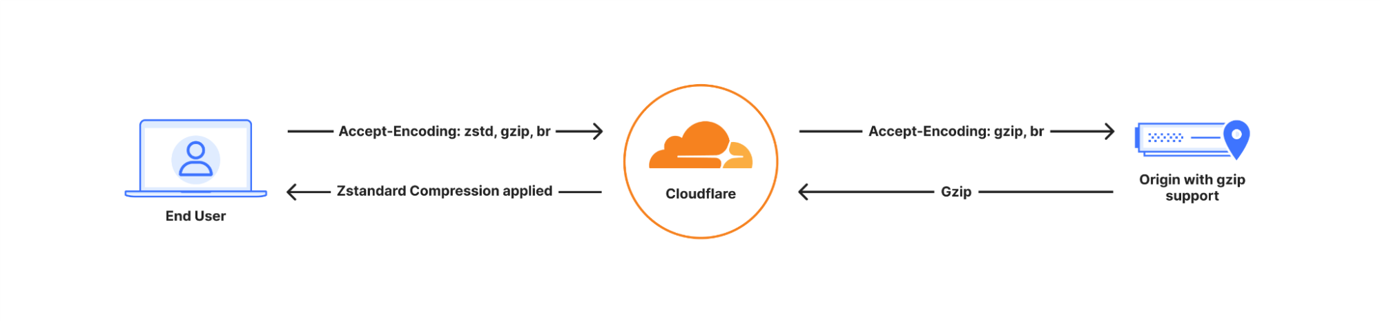
If the client does not support Zstandard, then Cloudflare will automatically fall back to Brotli, GZIP, or serve the content uncompressed where no compression algorithm is supported, ensuring compatibility.
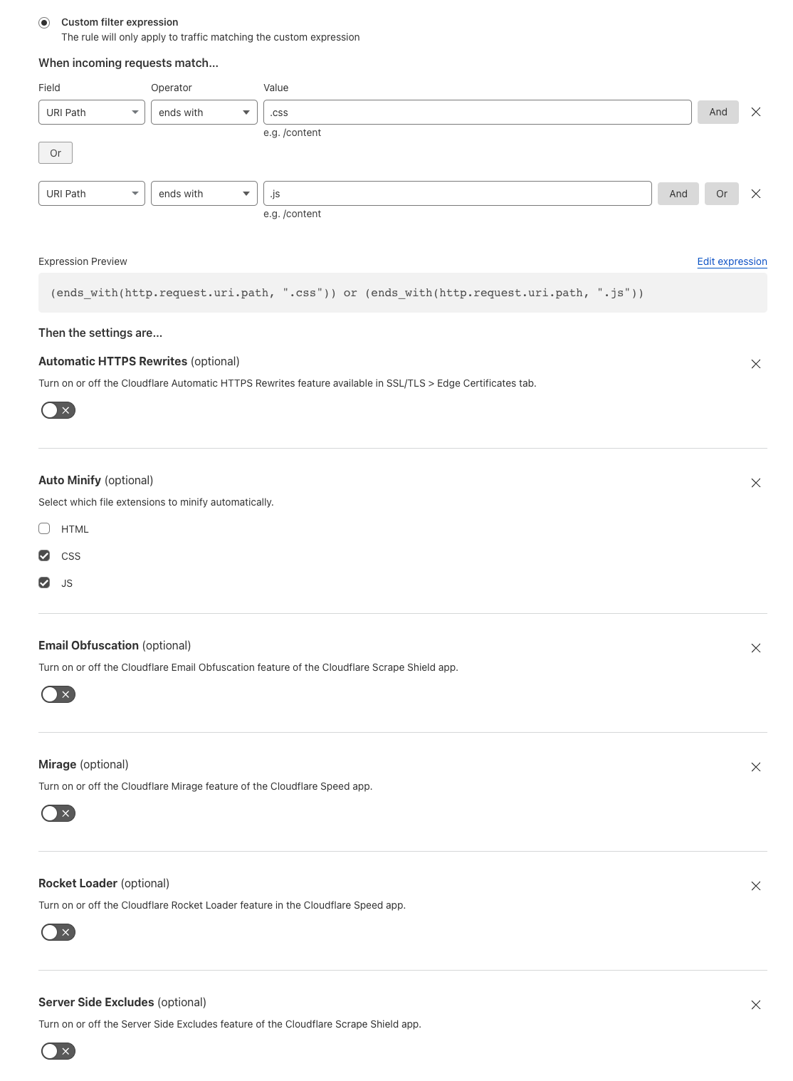
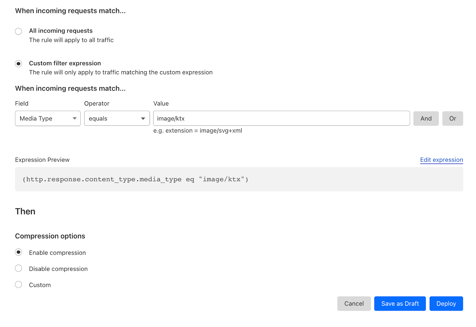
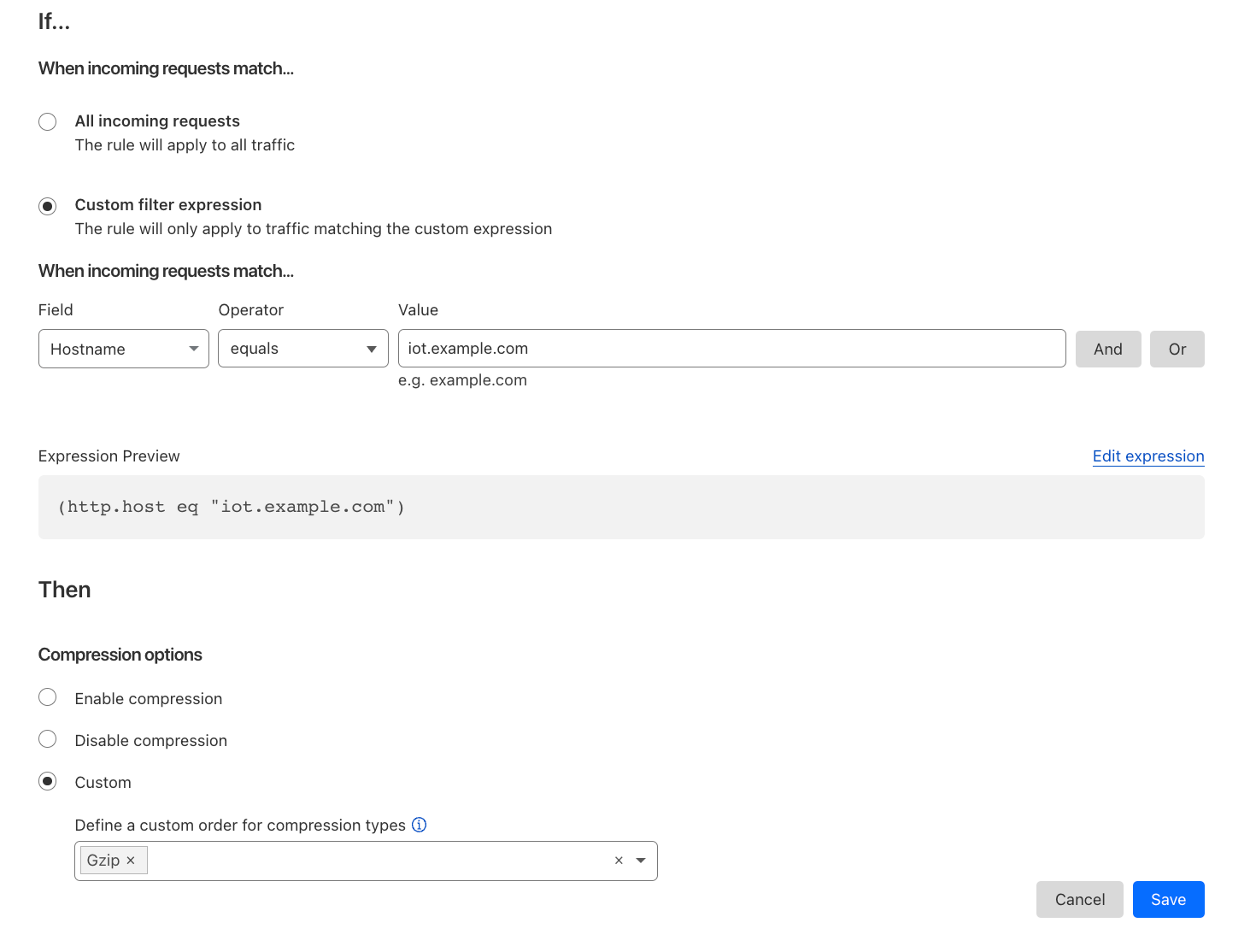
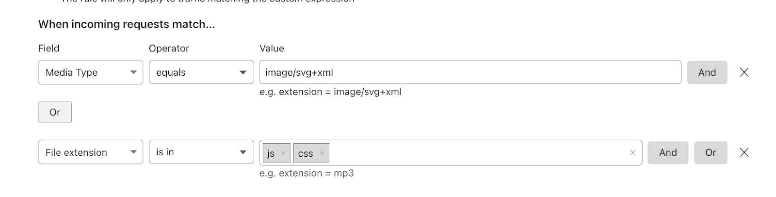
To enable Zstandard for your entire site or specifically filter on certain file types, all Cloudflare users can deploy a simple compression rule.
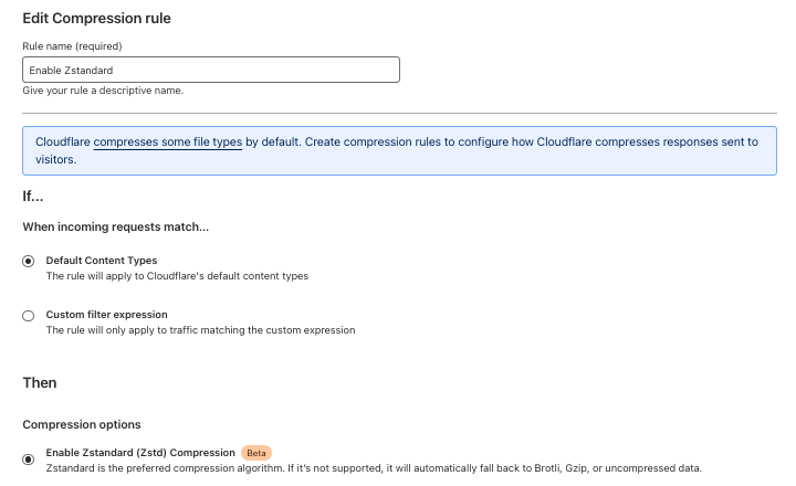
Further details and examples of what can be accomplished with Compression Rules can be found in our developer documentation.
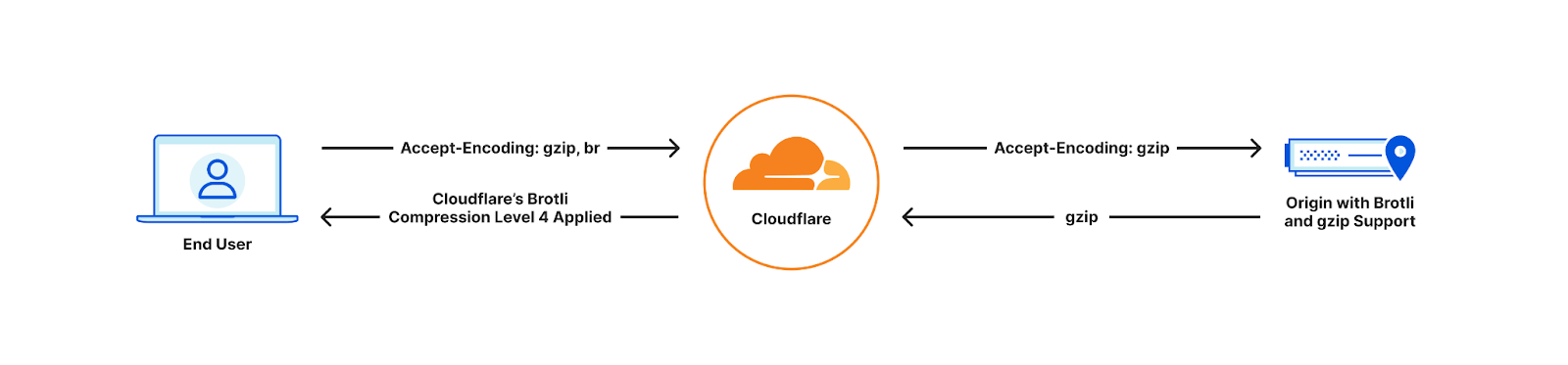
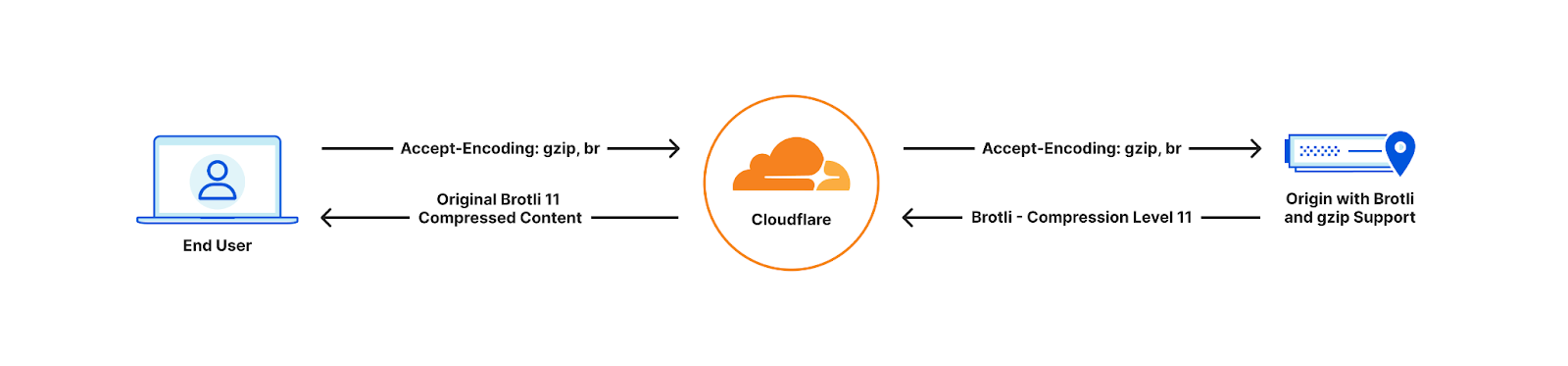
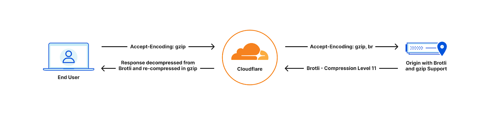
Currently, we support Zstandard, Brotli, and GZIP as compression algorithms for traffic sent to clients, and support GZIP and Brotli (since 2023) compressed data from the origin. We plan to implement full end-to-end support for Zstandard in 2025, offering customers another effective way to reduce their egress costs.
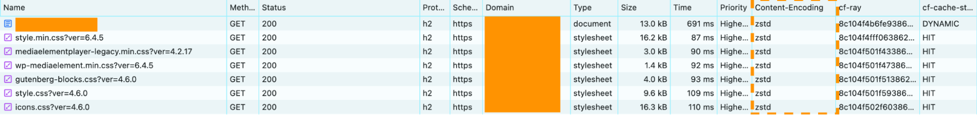
Once Zstandard is enabled, you can view your browser’s Network Activity log to check the content-encoding headers of the response.
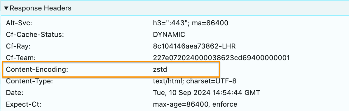
Enable Zstandard now!
Zstandard is now available to all Cloudflare customers through Compression Rules on our Enterprise and pay as you go plans, with free plans gaining access in October 2024. Whether you’re optimizing for speed or aiming to reduce bandwidth, Compression Rules give all customers granular control over their site’s performance.
Encrypted Client Hello (ECH)

While performance is crucial for delivering a fast user experience, ensuring privacy is equally important in today’s Internet landscape. As we optimize for speed with Zstandard, Cloudflare is also working to protect users’ sensitive information from being exposed during data transmission. With web traffic growing more complex and interconnected, it’s critical to keep both performance and privacy in balance. This is where technologies like Encrypted Client Hello (ECH) come into play, securing connections without sacrificing speed.
Ten years ago, we embarked on a mission to create a more secure and encrypted web. At the time, much of the Internet remained unencrypted, leaving user data vulnerable to interception. On September 27, 2014, we took a major step forward by enabling HTTPS for free for all Cloudflare customers. Overnight, we doubled the size of the encrypted web. This set the stage for a more secure Internet, ensuring that encryption was not a privilege limited by budget but a right accessible to everyone.
Since then, both Cloudflare and the broader community have helped encrypt more of the Internet. Projects like Let’s Encrypt launched to make certificates free for everyone. Cloudflare invested to encrypt more of the connection, and future-proof that encryption from coming technologies like quantum computers. We’ve always believed that it was everyone’s right, regardless of your budget, to have an encrypted Internet at no cost.
One of the last major challenges has been securing the SNI (Server Name Identifier), which remains exposed in plaintext during the TLS handshake. This is where Encrypted Client Hello (ECH) comes in, and today, we are proud to announce that we’re closing that gap.
Cloudflare announced support for Encrypted Client Hello (ECH) in 2023 and has continued to enhance its implementation in collaboration with our Internet browser partners. During a TLS handshake, one of the key pieces of information exchanged is the Server Name Identifier (SNI), which is used to initiate a secure connection. Unfortunately, the SNI is sent in plaintext, meaning anyone can read it. Imagine hand-delivering a letter — anyone following you can see where you’re delivering it, even if they don’t know the contents. With ECH, it is like sending the same confidential letter to a P.O. Box. You place your sensitive letter in a sealed inner envelope with the actual address. Then, you put that envelope into a larger, standard envelope addressed to a public P.O. Box, trusted to securely forward your intended recipient. The larger envelope containing the non-sensitive information is visible to everyone, while the inner envelope holds the confidential details, such as the actual address and recipient. Just as the P.O. Box maintains the anonymity of the true recipient’s address, ECH ensures that the SNI remains protected.
While encrypting the SNI is a primary motivation for ECH, its benefits extend further. ECH encrypts the entire TLS handshake, ensuring user privacy and enabling TLS to evolve without exposing sensitive connection data. By securing the full handshake, ECH allows for flexible, future-proof encryption designs that safeguard privacy as the Internet continues to grow.
How ECH works
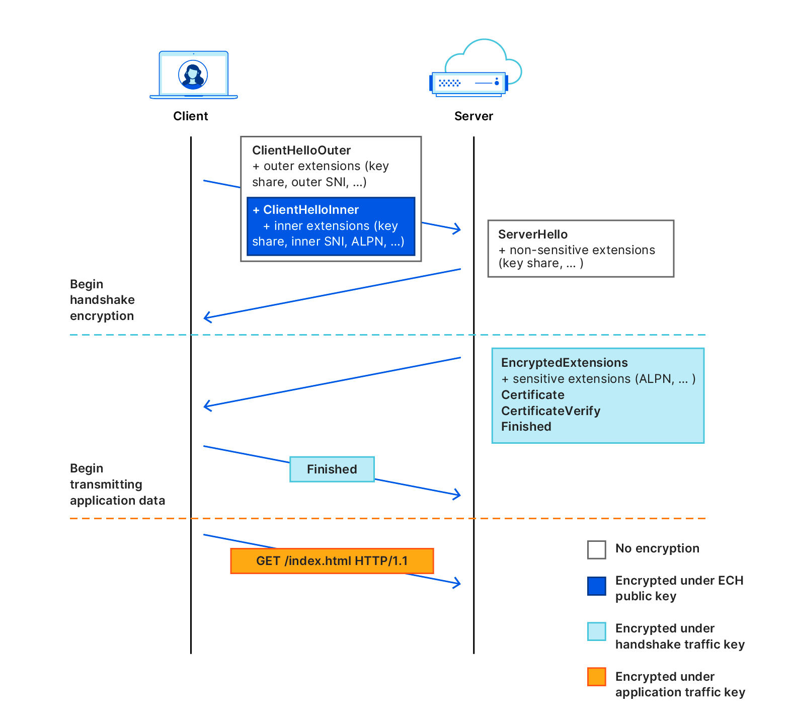
Encrypted Client Hello (ECH) introduces a layer of privacy by dividing the ClientHello message into two distinct parts: an outer ClientHello and an inner ClientHello.
-
Outer ClientHello: This part remains unencrypted and contains general information such as the list of ciphers and the TLS version. It includes a placeholder SNI, which is a common name used across Cloudflare’s network. For instance, all ECH-enabled websites on Cloudflare share the SNI
cloudflare-ech.com. Cloudflare manages this domain and possesses the necessary certificates to handle TLS negotiations for it. -
Inner ClientHello: This part is encrypted and includes the actual server name the client wants to visit. Encryption ensures that this sensitive data can only be decrypted by Cloudflare.
During the TLS handshake, the outer ClientHello reveals only the placeholder SNI (e.g., cloudflare-ech.com), while the encrypted inner ClientHello carries the real server name. As a result, intermediaries observing the traffic will only see the generic outer ClientHello, concealing the actual destination.
The design of ECH effectively addresses many challenges in securely deploying handshake encryption, thanks to the collaborative efforts within the IETF community. The key to ECH’s success is its integration with other IETF standards, including the new HTTPS DNS resource record, which enables HTTPS endpoints to advertise different TLS capabilities and simplifies key distribution. By using Encrypted DNS methods, browsers and clients can anonymously query these HTTPS records. These records contain the ECH parameters needed to initiate a secure connection.
ECH leverages the Hybrid Public Key Encryption (HPKE) standard, which streamlines the handshake encryption process, making it more secure and easier to implement. Before initiating a TCP connection, the user’s browser makes a DNS request for an HTTPS record, and zones with ECH enabled will include an ECH configuration in the HTTPS record containing an encryption public key and some associated metadata. For example, looking at the zone cloudflare-ech.com, you can see the following record returned:
dig cloudflare-ech.com https +short


1 . alpn="h3,h2" ipv4hint=104.18.10.118,104.18.11.118 ech=AEX+DQBB2gAgACD1W1B+GxY3nZ53Rigpsp0xlL6+80qcvZtgwjsIs4YoOwAEAAEAAQASY2xvdWRmbGFyZS1lY2guY29tAAA= ipv6hint=2606:4700::6812:a76,2606:4700::6812:b76
Aside from the public key used by the client to encrypt ClientHelloInner and other parameters that specify the ECH configuration, the ClientOuterHello is also present.
Y2xvdWRmbGFyZS1lY2guY29tWhen the string is decoded it reveals:
cloudflare-ech.comThis indicates the public outer SNI endpoint and where the TLS handshake should be forwarded to.
Practical implications
With ECH, any observer monitoring the traffic between the client and Cloudflare will see only uniform TLS handshakes that appear to be directed towards cloudflare-ech.com, regardless of the actual website being accessed. For instance, if a user visits example.com, intermediaries will not discern this specific destination but will only see cloudflare-ech.com in the visible handshake data.
The problem with middleboxes
In a basic HTTPS connection, a browser (client) establishes a TLS connection directly with an origin server to send requests and download content. However, many connections on the Internet do not go directly from a browser to the server but instead pass through some form of proxy or middlebox (often referred to as a “monster-in-the-middle” or MITM). This routing through intermediaries can occur for various reasons, both benign and malicious.
One common type of HTTPS interceptor is the TLS-terminating forward proxy. This proxy sits between the client and the destination server, transparently forwarding and potentially modifying traffic. To perform this task, the proxy terminates the TLS connection from the client, decrypts the traffic, and then re-encrypts and forwards it to the destination server over a new TLS connection. To avoid browser certificate validation errors, these forward proxies typically require users to install a root certificate on their devices. This root certificate allows the proxy to generate and present a trusted certificate for the destination server, a process often managed by network administrators in corporate environments, as seen with Cloudflare WARP. These services can help prevent sensitive company data from being transmitted to unauthorized destinations, safeguarding confidentiality.

However, TLS-terminating forward proxies are not equipped to handle Encrypted Client Hello (ECH) correctly. ECH separates the ClientHello message into an outer, unencrypted message and an inner, encrypted message. Since the proxy terminates the TLS connection and decrypts the traffic, it cannot manage or re-encrypt these messages as intended by ECH. Consequently, the proxy’s intervention can disrupt the ECH mechanism, potentially causing connection failures.
We also observed that specific Cloudflare setups, such as CNAME Flattening and Orange-to-Orange configurations, could cause ECH to break. This issue arose because the end destination for these requests did not support TLS 1.3, preventing ECH from being processed correctly. Fortunately, in close collaboration with our browser partners, we implemented a fallback in our BoringSSL implementation that handles TLS terminations. This fallback allows browsers to retry connections over TLS 1.2 without ECH, ensuring that a connection can be established and not break.
As a result of these improvements, we have enabled ECH by default for all Free plans, while all other plan types can manually enable it through their Cloudflare dashboard or via the API. We are excited to support ECH at scale, enhancing the privacy and security of users’ browsing activities. ECH plays a crucial role in safeguarding online interactions from potential eavesdroppers and maintaining the confidentiality of web activities.
HTTP/3 Prioritization and QUIC congestion control
Two other areas we are investing in to improve performance for all our customers are HTTP/3 Prioritization and QUIC congestion control.
HTTP/3 Prioritization focuses on efficiently managing the order in which web assets are loaded, thereby improving web performance by ensuring critical assets are delivered faster. HTTP/3 Prioritization uses Extensible Priorities to simplify prioritization with two parameters: urgency (ranging from 0-7) and a true/false value indicating whether the resource can be processed progressively. This allows resources like HTML, CSS, and images to be prioritized based on importance.
On the other hand, QUIC congestion control aims to optimize the flow of data, preventing network bottlenecks and ensuring smooth, reliable transmission even under heavy traffic conditions.
Both of these improvements significantly impact how Cloudflare’s network serves requests to clients. Before deploying these technologies across our global network, which handles peak traffic volumes of over 80 million requests per second, we first developed a reliable method to measure their impact through rigorous experimentation.
Measuring impact
Accurately measuring the impact of features implemented by Cloudflare for our customers is crucial for several reasons. These measurements ensure that optimizations related to performance, security, or reliability deliver the intended benefits without introducing new issues. Precise measurement validates the effectiveness of these changes, allowing Cloudflare to assess improvements in metrics such as load times, user experience, and overall site security. One of the best ways to measure performance changes is through aggregated real-world data.
Cloudflare Web Analytics offers free, privacy-first analytics for your website, helping you understand the performance of your web pages as experienced by your visitors. Real User Metrics (RUM) is a vital tool in web performance optimization, capturing data from real users interacting with a website, providing insights into site performance under real-world conditions. RUM tracks various metrics directly from the user’s device, including load times, resource usage, and user interactions. This data is essential for understanding the actual user experience, as it reflects the diverse environments and conditions under which the site is accessed.
A key performance indicator measured through RUM is Core Web Vitals (CWV), a set of metrics defined by Google that quantify crucial aspects of user experience on the web. CWV focuses on three main areas: loading performance, interactivity, and visual stability. The specific metrics include Largest Contentful Paint (LCP), which measures loading performance; First Input Delay (FID), which gauges interactivity; and Cumulative Layout Shift (CLS), which assesses visual stability. By using the CWV measurement in RUM, developers can monitor and optimize their applications to ensure a smoother, faster, and more stable user experience and track the impact of any changes they release.
Over the last three months we have developed the capability to include valuable information in Server-Timing response headers. When a page that uses Cloudflare Web Analytics is loaded in a browser, the privacy-first client-side script from Web Analytics collects browser metrics and server-timing headers, then sends back this performance data. This data is ingested, aggregated, and made available for querying. The server-timing header includes Layer 4 information, such as Round-Trip Time (RTT) and protocol type (TCP or QUIC). Combined with Core Web Vitals data, this allows us to determine whether an optimization has positively impacted a request compared to a control sample. This capability enables us to release large-scale changes such as HTTP/3 Prioritization or BBR with a clear understanding of their impact across our global network.
An example of this header contains several key properties that provide valuable information about the network performance as observed by the server:
server-timing: cfL4;desc="?proto=TCP&rtt=7337&sent=8&recv=8&lost=0&retrans=0&sent_bytes=3419&recv_bytes=832&delivery_rate=548023&cwnd=25&unsent_bytes=0&cid=94dae6b578f91145&ts=225-
proto: Indicates the transport protocol used
-
rtt: Round-Trip Time (RTT), representing the duration of the network round trip as measured by the layer 4 connection using a smoothing algorithm.
-
sent: Number of packets sent.
-
recv: Number of packets received.
-
lost: Number of packets lost.
-
retrans: Number of retransmitted packets.
-
sent_bytes: Total number of bytes sent.
-
recv_bytes: Total number of bytes received.
-
delivery_rate: Rate of data delivery, an instantaneous measurement in bytes per second.
-
cwnd: Congestion Window, an instantaneous measurement of packet or byte count depending on the protocol.
-
unsent_bytes: Number of bytes not yet sent.
-
cid: A 16-byte hexadecimal opaque connection ID.
-
ts: Timestamp in milliseconds, representing when the data was captured.
This real-time collection of performance data via RUM and Server-Timing headers allows Cloudflare to make data-driven decisions that directly enhance user experience. By continuously analyzing these detailed network and performance insights, we can ensure that future optimizations, such as HTTP/3 Prioritization or BBR deployment, are delivering tangible benefits for our customers.
Enabling HTTP/3 Prioritization for all plans
As part of our focus on improving observability through the integration of the server-timing header, we implemented several minor changes to optimize QUIC handshakes. Notably, we observed positive improvements in our telemetry due to the Layer 4 observability enhancements provided by the server-timing header. These internal findings coincided with third-party measurements, which showed similar improvements in handshake performance.
In the fourth quarter of 2024, we will apply the same experimental methodology to the HTTP/3 Prioritization support announced during Speed Week 2023. HTTP/3 Prioritization is designed to enhance the efficiency and speed of loading web pages by intelligently managing the order in which web assets are delivered to users. This is crucial because modern web pages are composed of numerous elements — such as images, scripts, and stylesheets — that vary in importance. Proper prioritization ensures that critical elements, like primary content and layout, load first, delivering a faster and more seamless browsing experience.
We will use this testing framework to measure performance improvements before enabling the feature across all plan types. This process allows us not only to quantify the benefits but, most importantly, to ensure there are no performance regressions.
Congestion control
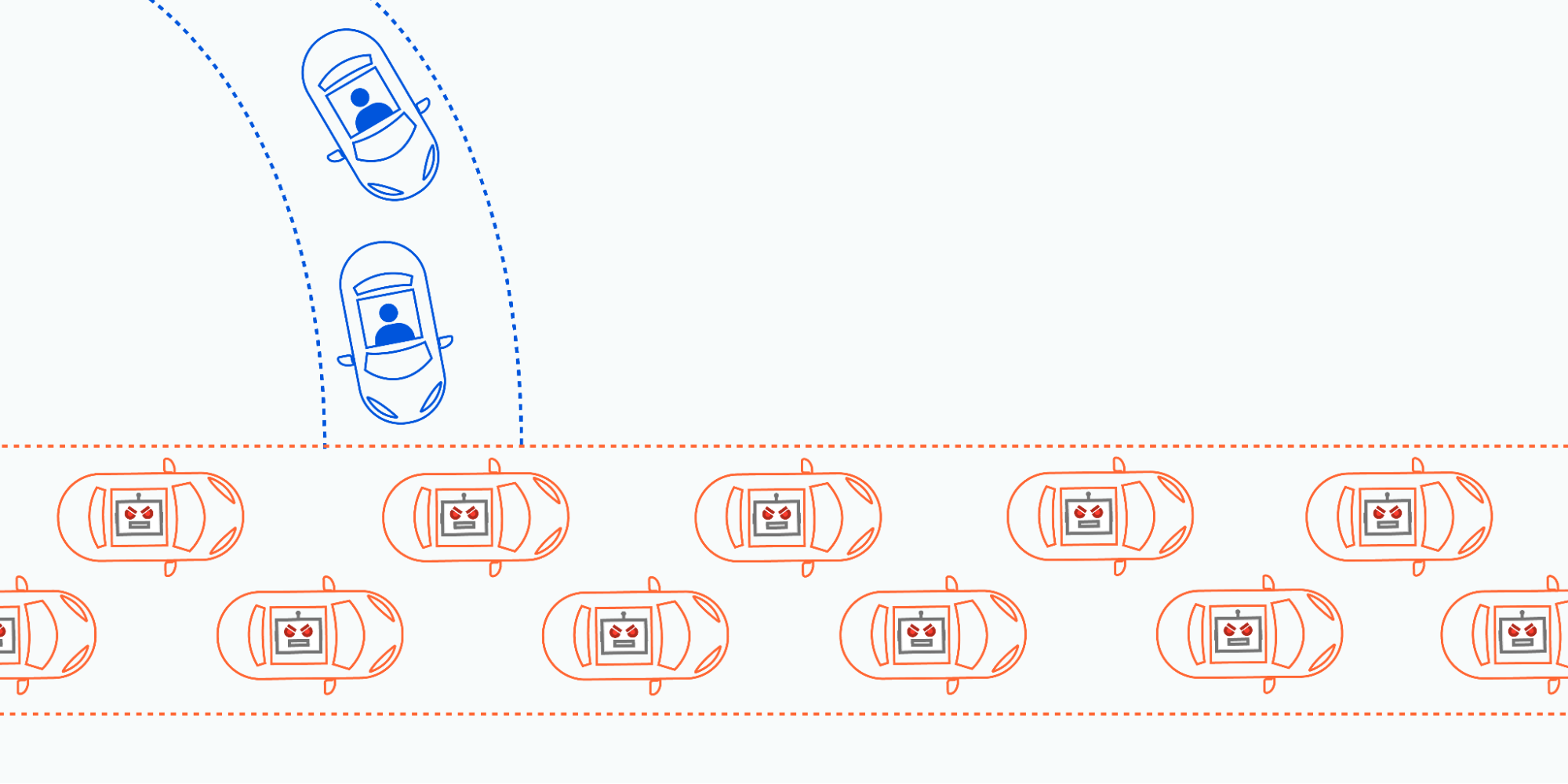
Following the completion of the HTTP/3 Prioritization experiments we will then begin testing different congestion control algorithms, specifically focusing on BBR (Bottleneck Bandwidth and Round-trip propagation time) version 3. Congestion control is a crucial mechanism in network communication that aims to optimize data transfer rates while avoiding network congestion. When too much data is sent too quickly over a network, it can lead to congestion, causing packet loss, delays, and reduced overall performance. Think of a busy highway during rush hour. If too many cars (data packets) flood the highway at once, traffic jams occur, slowing everyone down.
Congestion control algorithms act like traffic managers, regulating the flow of data to prevent these “traffic jams,” ensuring that data moves smoothly and efficiently across the network. Each side of a connection runs an algorithm in real time, dynamically adjusting the flow of data based on the current and predicted network conditions.
BBR is an advanced congestion control algorithm, initially developed by Google. BBR seeks to estimate the actual available bandwidth and the minimum round-trip time (RTT) to determine the optimal data flow. This approach allows BBR to maintain high throughput while minimizing latency, leading to more efficient and stable network performance.
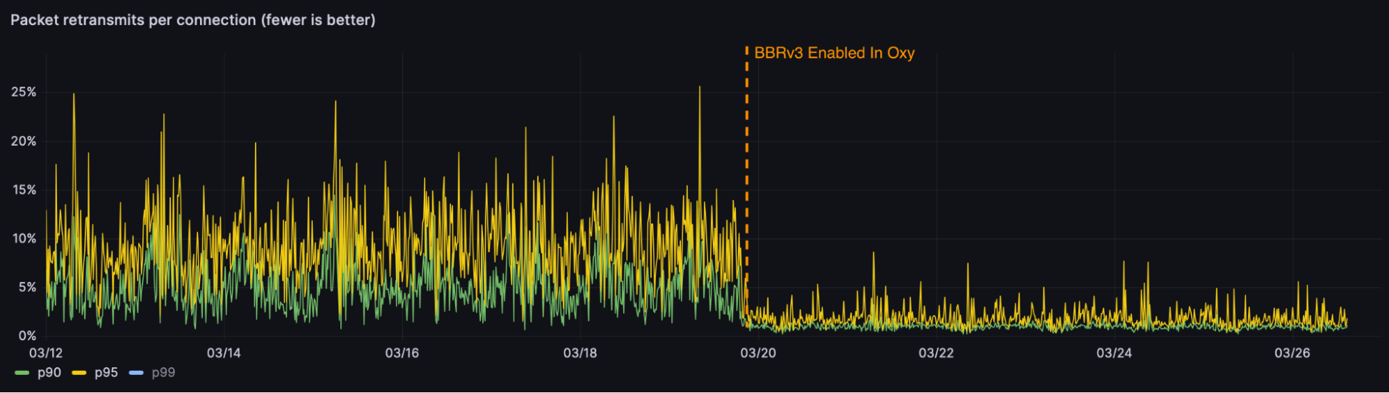
BBR v3, the latest iteration, builds on the strengths of its predecessors BBRv1 and BBRv2 by further refining its bandwidth estimation techniques and enhancing its adaptability to varying network conditions. We found BBR v3 to be faster in several cases compared to our previous implementation of CUBIC. Most importantly, it reduced loss and retransmission rates in our Oxy proxy implementation.
With these promising results, we are excited to test various congestion control algorithms including BBRv3 for quiche, our QUIC implementation, across our HTTP/3 traffic. Combining the layer 4 server-timing information with experiments in this area will enable us to explicitly control and measure the impact on real-world metrics.
The future
The future of the Internet relies on continuous innovation to meet the growing demands for speed, security, and scalability. Technologies like Zstandard for compression, BBR for congestion control, HTTP/3 prioritization, and Encrypted Client Hello are setting new standards for performance and privacy. By implementing these protocols, web services can achieve faster page load times, more efficient bandwidth usage, and stronger protections for user data.
These advancements don’t just offer incremental improvements, they provide a significant leap forward in optimizing the user experience and safeguarding online interactions. At Cloudflare, we are committed to making these technologies accessible to everyone, empowering businesses to deliver better, faster, and more secure services.
Stay tuned for more developments as we continue to push the boundaries of what’s possible on the web and if you’re passionate about building and implementing the latest Internet innovations, we’re hiring!