Cloudflare operates the fastest network on the planet. We’ve shared an update today about how we are overhauling the software technology that accelerates every server in our fleet, improving speed globally.
That is not where the work stops, though. To improve speed even further, we have to also make sure that our network swiftly handles the Internet-scale congestion that hits it every day, routing traffic to our now-faster servers.
We have invested in congestion control for years. Today, we are excited to share how we are applying a superpower of our network, our massive Free Plan user base, to optimize performance and find the best way to route traffic across our network for all our customers globally.
Early results have seen performance increases that average 10% faster than the prior baseline. We achieved this by applying different algorithmic methods to improve performance based on the data we observe about the Internet each day. We are excited to begin rolling out these improvements to all customers.
How does traffic arrive in our network?
The Internet is a massive collection of interconnected networks, each composed of many machines (“nodes”). Data is transmitted by breaking it up into small packets, and passing them from one machine to another (over a “link”). Each one of these machines is linked to many others, and each link has limited capacity.
When we send a packet over the Internet, it will travel in a series of “hops” over the links from A to B. At any given time, there will be one link (one “hop”) with the least available capacity for that path. It doesn’t matter where in the connection this hop is — it will be the bottleneck.
But there’s a challenge — when you’re sending data over the Internet, you don’t know what route it’s going to take. In fact, each node decides for itself which route to send the traffic through, and different packets going from A to B can take entirely different routes. The dynamic and decentralized nature of the system is what makes the Internet so effective, but it also makes it very hard to work out how much data can be sent. So — how can a sender know where the bottleneck is, and how fast to send data?
Between Cloudflare nodes, our Argo Smart Routing product takes advantage of our visibility into the global network to speed up communication. Similarly, when we initiate connections to customer origins, we can leverage Argo and other insights to optimize them. However, the speed of a connection from your phone or laptop (the Client below) to the nearest Cloudflare datacenter will depend on the capacity of the bottleneck hop in the chain from you to Cloudflare, which happens outside our network.
What happens when too much data arrives at once?
If too much data arrives at any one node in a network in the path of a request being processed, the requestor will experience delays due to congestion. The data will either be queued for a while (risking bufferbloat), or some of it will simply get dropped. Protocols like TCP and QUIC respond to packets being dropped by retransmitting the data, but this introduces a delay, and can even make the problem worse by further overloading the limited capacity.
If cloud infrastructure providers like Cloudflare don’t manage congestion carefully, we risk overloading the system, slowing down the rate of data getting through. This actually happened in the early days of the Internet. To avoid this, the Internet infrastructure community has developed systems for controlling congestion, which give everyone a turn to send their data, without overloading the network. This is an evolving challenge, as the network grows ever more complicated, and the best method to implement congestion control is a constant pursuit. Many different algorithms have been developed, which take different sources of information and signals, optimize in a particular method, and respond to congestion in different ways.
Congestion control algorithms use a number of signals to estimate the right rate to send traffic, without knowing how the network is set up. One important signal has been loss. When a packet is received, the receiver sends an “ACK,” telling the sender the packet got through. If it’s dropped somewhere along the way, the sender never gets the receipt, and after a timeout will treat the packet as having been lost.
More recent algorithms have used additional data. For example, a popular algorithm called BBR (Bottleneck Bandwidth and Round-trip propagation time), which we have been using for much of our traffic, attempts to build a model during each connection of the maximum amount of data that can be transmitted in a given time period, using estimates of the round trip time as well as loss information.
The best algorithm to use often depends on the workload. For example, for interactive traffic like a video call, an algorithm that biases towards sending too much traffic can cause queues to build up, leading to high latency and poor video experience. If one were to optimize solely for that use case though, and avoid that by sending less traffic, the network will not make the best use of the connection for clients doing bulk downloads. The performance optimization outcome varies, depending on a lot of different factors. But – we have visibility into many of them!
BBR was an exciting development in congestion control approach, moving from reactive loss-based approaches to proactive model-based optimization, resulting in significantly better performance for modern networks. Our data gives us an opportunity to go further, applying different algorithmic methods to improve performance.
How can we do better?
All the existing algorithms are constrained to use only information gathered during the lifetime of the current connection. Thankfully, we know far more about the Internet at any given moment than this! With Cloudflare’s perspective on traffic, we see much more than any one customer or ISP might see at any given time.
Every day, we see traffic from essentially every major network on the planet. When a request comes into our system, we know what client device we’re talking to, what type of network is enabling the connection, and whether we’re talking to consumer ISPs or cloud infrastructure providers.
We know about the patterns of load across the global Internet, and the locations where we believe systems are overloaded, within our network, or externally. We know about the networks that have stable properties, which have high packet loss due to cellular data connections, and the ones that traverse low earth orbit satellite links and radically change their routes every 15 seconds.
How does this work?
We have been in the process of migrating our network technology stack to use a new platform, powered by Rust, that provides more flexibility to experiment with varying the parameters in the algorithms used to handle congestion control. Then we needed data.
The data powering these experiments needs to reflect the measure we’re trying to optimize, which is the user experience. It’s not just enough that we’re sending data to nearly all the networks on the planet; we have to be able to see what is the experience that customers have. So how do we do that, at our scale?
First, we have detailed “passive” logs of the rate at which data is able to be sent from our network, and how long it takes for the destination to acknowledge receipt. This covers all our traffic, and gives us an idea of how quickly the data was received by the client, but doesn’t guarantee to tell us about the user experience.
Next, we have a system for gathering Real User Measurement (RUM) data, which records information in supported web browsers about metrics such as Page Load Time (PLT). Any Cloudflare customer can enable this and will receive detailed insights in their dashboard. In addition, we use this metadata in aggregate across all our customers and networks to understand what customers are really experiencing.
However, RUM data is only going to be present for a small proportion of connections across our network. So, we’ve been working to find a way to predict the RUM measures by extrapolating from the data we see only in passive logs. For example, here are the results of an experiment we performed comparing two different algorithms against the cubic baseline.
Now, here’s the same timescale, observed through the prediction based on our passive logs. The curves are very similar – but even more importantly, the ratio between the curves is very similar. This is huge! We can use a relatively small amount of RUM data to validate our findings, but optimize our network in a much more fine-grained way by using the full firehose of our passive logs.
Extrapolating too far becomes unreliable, so we’re also working with some of our largest customers to improve our visibility of the behaviour of the network from their clients’ point of view, which allows us to extend this predictive model even further. In return, we’ll be able to give our customers insights into the true experience of their clients, in a way that no other platform can offer.
What is next?
We’re currently running our experiments and improved algorithms for congestion control on all of our free tier QUIC traffic. As we learn more, verify on more complex customers, and expand to TCP traffic, we’ll gradually roll this out to all our customers, for all traffic, over 2026 and beyond. The results have led to as much as a 10% improvement as compared to the baseline!
We’re working with a select group of enterprises to test this in an early access program. If you’re interested in learning more, contact us!
There’s a tradition at Cloudflare of launching real products on April 1, instead of the usual joke product announcements circulating online today. In previous years, we’ve introduced impactful products like 1.1.1.1 and 1.1.1.1 for Families. Today, we’re excited to continue this tradition by making every purge method available to all customers, regardless of plan type.
During Birthday Week 2024, we announced our intention to bring the full suite of purge methods — including purge by URL, purge by hostname, purge by tag, purge by prefix, and purge everything — to all Cloudflare plans. Historically, methods other than “purge by URL” and “purge everything” were exclusive to Enterprise customers. However, we’ve been openly rebuilding our purge pipeline over the past few years (hopefully you’ve read some of ourblogseries), and we’re thrilled to share the results more broadly. We’ve spent recent months ensuring the new Instant Purge pipeline performs consistently under 150 ms, even during increased load scenarios, making it ready for every customer.
But that’s not all — we’re also significantly raising the default purge rate limits for Enterprise customers, allowing even greater purge throughput thanks to the efficiency of our newly developed Instant Purge system.
Building a better purge: a two-year journey
Stepping back, today’s announcement represents roughly two years of focused engineering. Near the end of 2022, our team went heads down rebuilding Cloudflare’s purge pipeline with a clear yet challenging goal: dramatically increase our throughput while maintaining near-instant invalidation across our global network.
Cloudflare operates data centers in over 335 cities worldwide. Popular cached assets can reside across all of our data centers, meaning each purge request must quickly propagate to every location caching that content. Upon receiving a purge command, each data center must efficiently locate and invalidate cached content, preventing stale responses from being served. The amount of content that must be invalidated can vary drastically, from a single file, to all cached assets associated with a particular hostname. After the content has been purged, any subsequent requests will trigger retrieval of a fresh copy from the origin server, which will be stored in Cloudflare’s cache during the response.
Ensuring consistent, rapid propagation of purge requests across a vast network introduces substantial technical challenges, especially when accounting for occasional data center outages, maintenance, or network interruptions. Maintaining consistency under these conditions requires robust distributed systems engineering.
How did we scale purge?
We’ve previously discussed how our new Instant Purge system was architected to achieve sub-150 ms purge times. It’s worth noting that the performance improvements were only part of what our new architecture achieved, as it also helped us solve significant scaling challenges around storage and throughput that allowed us to bring Instant Purge to all users.
Initially, our purge system scaled well, but with rapid customer growth, the storage consumption from millions of daily purge keys that needed to be stored reduced available caching space. Early attempts to manage this storage and throughput demand involved queues and batching for smoothing traffic spikes, but this introduced latency and underscored the tight coupling between increased usage and rising storage costs.
We needed to revisit our thinking on how to better store purge keys and when to remove purged content so we could reclaim space. Historically, when a customer would purge by tag, prefix or hostname, Cloudflare would mark the content as expired and allow it to be evicted later. This is known as lazy-purge because nothing is actively removed from disk. Lazy-purge is fast, but not necessarily efficient, because it consumes storage for expired but not-yet-evicted content. After examining global or data center-level indexing for purge keys, we decided that wasn’t viable due to increases in system complexity and the latency those indices could bring due to our network size. So instead, we opted for per-machine indexing, integrating indices directly alongside our cache proxies. This minimized network complexity, simplified reliability, and provided predictable scaling.
After careful analysis and benchmarking, we selected RocksDB, an embedded key-value store that we could optimize for our needs, which formed the basis of CacheDB, our Rust-based service running alongside each cache proxy. CacheDB manages indexing and immediate purge execution (active purge), significantly reducing storage needs and freeing space for caching.
Local queues within CacheDB buffer purge operations to ensure consistent throughput without latency spikes, while the cache proxies consult CacheDB to guarantee rapid, active purges. Our updated distribution pipeline broadcasts purges directly to CacheDB instances across machines, dramatically improving throughput and purge speed.
Using CacheDB, we’ve reduced storage requirements 10x by eliminating lazy purge storage accumulation, instantly freeing valuable disk space. The freed storage enhances cache retention, boosting cache HIT ratios and minimizing origin egress. These savings in storage and increased throughput allowed us to scale to the point where we can offer Instant Purge to more customers.
For more information on how we designed the new Instant Purge system, please see the previous installment of our Purge series blog posts.
Striking the right balance: what to purge and when
Moving on to practical considerations of using these new purge methods, it’s important to use the right method for what you want to invalidate. Purging too aggressively can overwhelm origin servers with unnecessary requests, driving up egress costs and potentially causing downtime. Conversely, insufficient purging leaves visitors with outdated content. Balancing precision and speed is vital.
Cloudflare supports multiple targeted purge methods to help customers achieve this balance.
Purge Everything: Clears all cached content associated with a website.
Purge by Tag: Uses Cache-Tag headers to invalidate grouped assets, offering flexibility for complex cache management scenarios.
Starting today, all of these methods are available to every Cloudflare customer.
How to purge
Users can select their purge method directly in the Cloudflare dashboard, located under the Cache tab in the configurations section, or via the Cloudflare API. Each purge request should clearly specify the targeted URLs, hostnames, prefixes, or cache tags relevant to the selected purge type (known as purge keys). For instance, a prefix purge request might specify a directory such as example.com/foo/bar. To maximize efficiency and throughput, batching multiple purge keys in a single request is recommended over sending individual purge requests each with a single key.
How much can you purge?
The new rate limits for Cloudflare’s purge by tag, prefix, hostname, and purge everything are different for each plan type. We use a token bucket rate limit system, so each account has a token bucket with a maximum size based on plan type. When we receive a purge request we first add tokens to the account’s bucket based on the time passed since the account’s last purge request divided by the refill rate for its plan type (which can be a fraction of a token). Then we check if there’s at least one whole token in the bucket, and if so we remove it and process the purge request. If not, the purge request will be rate limited. An easy way to think about this rate limit is that the refill rate represents the consistent rate of requests a user can send in a given period while the bucket size represents the maximum burst of requests available.
For example, a free user starts with a bucket size of 25 requests and a refill rate of 5 requests per minute (one request per 12 seconds). If the user were to send 26 requests all at once, the first 25 would be processed, but the last request would be rate limited. They would need to wait 12 seconds and retry their last request for it to succeed.
The current limits are applied per account:
Plan
Bucket size
Request refill rate
Max keys per request
Total keys
Free
25 requests
5 per minute
100
500 per minute
Pro
25 requests
5 per second
100
500 per second
Biz
50 requests
10 per second
100
1,000 per second
Enterprise
500 requests
50 per second
100
5,000 per second
More detailed documentation on all purge rate limits can be found in our documentation.
What’s next?
We’ve spent a lot of time optimizing our purge platform. But we’re not done yet. Looking forward, we will continue to enhance the performance of Cloudflare’s single-file purge. The current P50 performance is around 250 ms, and we suspect that we can optimize it further to bring it under 200 ms. We will also build out our ability to allow for greater purge throughput for all of our systems, and will continue to find ways to implement filtering techniques to ensure we can continue to scale effectively and allow customers to purge whatever and whenever they choose.
We invite you to try out our new purge system today and deliver an instant, seamless experience to your visitors.
Failure is an expected state in production systems, and no predictable failure of either software or hardware components should result in a negative experience for users. The exact failure mode may vary, but certain remediation steps must be taken after detection. A common example is when an error occurs on a server, rendering it unfit for production workloads, and requiring action to recover.
When operating at Cloudflare’s scale, it is important to ensure that our platform is able to recover from faults seamlessly. It can be tempting to rely on the expertise of world-class engineers to remediate these faults, but this would be manual, repetitive, unlikely to produce enduring value, and not scaling. In one word: toil; not a viable solution at our scale and rate of growth.
In this post we discuss how we built the foundations to enable a more scalable future, and what problems it has immediately allowed us to solve.
Growing pains
The Cloudflare Site Reliability Engineering (SRE) team builds and manages the platform that helps product teams deliver our extensive suite of offerings to customers. One important component of this platform is the collection of servers that power critical products such as Durable Objects, Workers, and DDoS mitigation. We also build and maintain foundational software services that power our product offerings, such as configuration management, provisioning, and IP address allocation systems.
As part of tactical operations work, we are often required to respond to failures in any of these components to minimize impact to users. Impact can vary from lack of access to a specific product feature, to total unavailability. The level of response required is determined by the priority, which is usually a reflection of the severity of impact on users. Lower-priority failures are more common — a server may run too hot, or experience an unrecoverable hardware error. Higher-priority failures are rare and are typically resolved via a well-defined incident response process, requiring collaboration with multiple other teams.
The commonality of lower-priority failures makes it obvious when the response required, as defined in runbooks, is “toilsome”. To reduce this toil, we had previously implemented a plethora of solutions to automate runbook actions such as manually-invoked shell scripts, cron jobs, and ad-hoc software services. These had grown organically over time and provided solutions on a case-by-case basis, which led to duplication of work, tight coupling, and lack of context awareness across the solutions.
We also care about how long it takes to resolve any potential impact on users. A resolution process which involves the manual invocation of a script relies on human action, increasing the Mean-Time-To-Resolve (MTTR) and leaving room for human error. This risks increasing the amount of errors we serve to users and degrading trust.
These problems proved that we needed a way to automatically heal these platform components. This especially applies to our servers, for which failure can cause impact across multiple product offerings. While we have mechanisms to automatically steer traffic away from these degraded servers, in some rare cases the breakage is sudden enough to be visible.
Solving the problem
To provide a more reliable platform, we needed a new component that provides a common ground for remediation efforts. This would remove duplication of work, provide unified context-awareness and increase development speed, which ultimately saves hours of engineering time and effort.
A good solution would not allow only the SRE team to auto-remediate, it would empower the entire company. The key to adding self-healing capability was a generic interface for all teams to self-service and quickly remediate failures at various levels: machine, service, network, or dependencies.
A good way to think about auto-remediation is in terms of workflows. A workflow is a sequence of steps to get to a desired outcome. This is not dissimilar to a manual shell script which executes what a human would otherwise do via runbook instructions. Because of this logical fit with workflows, we decided to adopt Temporal.
Temporal is a durable execution platform which is useful to gracefully manage infrastructure failures such as network outages and transient failures in external service endpoints. This capability meant we only needed to build a way to schedule “workflow” tasks and have Temporal provide reliability guarantees. This allowed us to focus on building out the orchestration system to support the control and flow of workflow execution in our data centers.
How does Temporal work?
Before we discuss the system that provides our self-healing functions, let’s explore how the workflow execution engine works, as its native architecture provided numerous benefits that we took advantage of to build a more robust foundation.
The most attractive feature Temporal offered us was the ability to write code that has reliability baked in. Some examples of these primitives are automatic retries, timeouts, rollbacks, and queueing. The Temporal Platform consists of the Temporal Cluster and Worker processes (application code that contains your custom logic).
This architecture allowed us to write our application logic as we normally would, with the added benefits of Temporal. Since Temporal Workers are external to the cluster, we can run tasks anywhere across our global network — a feature that made it easy to build an extensible, easy-to-understand framework for automating tasks.
In Temporal terms, control is provided by the basic principles used to provide workflow execution — Workflows and Activities. A Workflow is simply a sequence of Activities, which are functions that ideally do only ONE task, such as making a request to an external service or rebooting a machine.
Control of workflow behavior can be done using ActivityOptions. This is where you can define timeouts for workflow execution, retry policies, and task queues. Each worker can poll several task queues for both Workflow and Activity tasks. If no worker is polling the task queue in which a Workflow task is declared, nothing happens.
Below, we describe how our automatic remediation system works. It is essentially a way to schedule tasks across our global network with built-in reliability guarantees. With this system, teams can serve their customers more reliably. An unexpected failure mode can be recognized and immediately mitigated, while the root cause can be determined later via a more detailed analysis.
Step one: we need a coordinator
After our initial testing of Temporal, it was now possible to write workflows. But we needed a way to schedule workflow tasks from other internal services. The coordinator was built to serve this purpose, and became the primary mechanism for the authorisation and scheduling of workflows.
The most important roles of the coordinator are authorisation, workflow task routing, and safety constraints enforcement. Each consumer is authorized via mTLS authentication, and the coordinator uses an ACL to determine whether to permit the execution of a workflow. An ACL configuration looks like the following example.
Each workflow specifies two key characteristics: where to run the tasks and the safety constraints, using an HCL configuration file. Example constraints could be whether to run on only a specific node type (such as a database), or if multiple parallel executions are allowed: if a task has been triggered too many times, that is a sign of a wider problem that might require human intervention. The coordinator uses the Temporal Visibility API to determine the current state of the executions in the Temporal cluster.
An example of a configuration file is shown below:
task_queue_target = "<target>"

# The following entries will ensure that
# 1. This workflow is not run at the same time in a 15m window.
# 2. This workflow will not run more than once an hour.
# 3. This workflow will not run more than 3 times in one day.
#
constraint {
    kind = "concurency"
    value = "1"
    period = "15m"
}

constraint {
    kind = "maxExecution"
    value = "1"
    period = "1h"
}

constraint {
    kind = "maxExecution"
    value = "3"
    period = "24h"
    is_global = true
}
Step two: Task Routing is amazing
An unforeseen benefit of using a central Temporal cluster was the discovery of Task Routing. This feature allows us to schedule a Workflow/Activity on any server that has a running Temporal Worker, and further segment by the type of server, its location, etc. For this reason, we have three primary task queues — the general queue in which tasks can be executed by any worker in the datacenter, the node type queue in which tasks can only be executed by a specific node type in the datacenter, and the individual node queue where we target a specific node for task execution.
We rely on this heavily to ensure the speed and efficiency of automated remediation. Certain tasks can be run in datacenters with known low latency to an external resource, or a node type with better performance than others (due to differences in the underlying hardware). This reduces the amount of failure and latency we see overall in task executions. Sometimes we are also constrained by certain types of tasks that can only run on a certain node type, such as a database.
Task Routing also means that we can configure certain task queues to have a higher priority for execution, although this is not a feature we have needed so far. A drawback of task routing is that every Workflow/Activity needs to be registered to the target task queue, which is a common gotcha. Thankfully, it is possible to catch this failure condition with proper testing.
Step three: when/how to self-heal?
None of this would be relevant if we didn’t put it to good use. A primary design goal for the platform was to ensure we had easy, quick ways to trigger workflows on the most important failure conditions. The next step was to determine what the best sources to trigger the actions were. The answer to this was simple: we could trigger workflows from anywhere as long as they are properly authorized and detect the failure conditions accurately.
Example triggers are an alerting system, a log tailer, a health check daemon, or an authorized engineer via a chatbot. Such flexibility allows a high level of reuse, and permits to invest more in workflow quality and reliability.
As part of the solution, we built a daemon that is able to poll a signal source for any unwanted condition and trigger a configured workflow. We have initially found Prometheus useful as a source because it contains both service-level and hardware/system-level metrics. We are also exploring more event-based trigger mechanisms, which could eliminate the need to use precious system resources to poll for metrics.
We already had internal services that are able to detect widespread failure conditions for our customers, but were only able to page a human. With the adoption of auto-remediation, these systems are now able to react automatically. This ability to create an automatic feedback loop with our customers is the cornerstone of these self-healing capabilities and we continue to work on stronger signals, faster reaction times, and better prevention of future occurrences.
The most exciting part, however, is the future possibility. Every customer cares about any negative impact from Cloudflare. With this platform we can onboard several services (especially those that are foundational for the critical path) and ensure we react quickly to any failure conditions, even before there is any visible impact.
Step four: packaging and deployment
The whole system is written in golang, and a single binary can implement each role. We distribute it as an apt package or a container for maximum ease of deployment.
We deploy a Temporal-based worker to every server we intend to run tasks on, and a daemon in datacenters where we intend to automatically trigger workflows based on the local conditions. The coordinator is more nuanced since we rely on task routing and can trigger from a central coordinator, but we have also found value in running coordinators locally in the datacenters. This is especially useful in datacenters with less capacity or degraded performance, removing the need for a round-trip to schedule the workflows.
Step five: test, test, test
Temporal provides native mechanisms to test an entire workflow, via a comprehensive test suite that supports end-to-end, integration, and unit testing, which we used extensively to prevent regressions while developing. We also ensured proper test coverage for all the critical platform components, especially the coordinator.
Despite the ease of written tests, we quickly discovered that they were not enough. After writing workflows, engineers need an environment as close as possible to the target conditions. This is why we configured our staging environments to support quick and efficient testing. These environments receive the latest changes and point to a different (staging) Temporal cluster, which enables experimentation and easy validation of changes.
After a workflow is validated in the staging environment, we can then do a full release to production. It seems obvious, but catching simple configuration errors before releasing has saved us many hours in development/change-related-task time.
Deploying to production
As you can guess from the title of this post, we put this in production to automatically react to server-specific errors and unrecoverable failures. To this end, we have a set of services that are able to detect single-server failure conditions based on analyzed traffic data. After deployment, we have successfully mitigated potential impact by taking any errant single sources of failure out of production.
We have also created a set of workflows to reduce internal toil and improve efficiency. These workflows can automatically test pull requests on target machines, wipe and reset servers after experiments are concluded, and take away manual processes that cost many hours in toil.
Building a system that is maintained by several SRE teams has allowed us to iterate faster, and rapidly tackle long-standing problems. We have set ambitious goals regarding toil elimination and are on course to achieve them, which will allow us to scale faster by eliminating the human bottleneck.
Looking to the future
Our immediate plans are to leverage this system to provide a more reliable platform for our customers and drastically reduce operational toil, freeing up engineering resources to tackle larger-scale problems. We also intend to leverage more Temporal features such as Workflow Versioning, which will simplify the process of making changes to workflows by ensuring that triggered workflows run expected versions.
We are also interested in how others are solving problems using durable execution platforms such as Temporal, and general strategies to eliminate toil. If you would like to discuss this further, feel free to reach out on the Cloudflare Community and start a conversation!
Each time a user visits your web page, they are initiating a race to receive content as quickly as possible. Performance is a critical factor that influences how visitors interact with your site. Some might think that moving content across the globe introduces significant latency, but for a while, network transmission speeds have approached their theoretical limits. To put this into perspective, data on Cloudflare can traverse the 11,000 kilometer round trip between New York and London in about 76 milliseconds – faster than the blink of an eye.
However, delays in loading web pages persist due to the complexities of processing requests, responses, and configurations. In addition to pushing advancements in connection establishment, compression, hardware, and software, we have built a new way to reduce page load latency by anticipating how visitors will interact with a given web page.
Today we are very excited to share the latest leap forward in speed: Speed Brain. It relies on the Speculation Rules API to prefetch the content of the user’s likely next navigations. The main goal of Speed Brain is to download a web page to the browser cache before a user navigates to it, allowing pages to load almost instantly when the actual navigation takes place.
Our initial approach uses a conservative model that prefetches static content for the next page when a user starts a touch or click event. Through the fourth quarter of 2024 and into 2025, we will offer more aggressive speculation models, such as speculatively prerendering (not just fetching the page before the navigation happens but rendering it completely) for an even faster experience. Eventually, Speed Brain will learn how to eliminate latency for your static website, without any configuration, and work with browsers to make sure that it loads as fast as possible.
To illustrate, imagine an ecommerce website selling clothing. Using the insights from our global request logs, we can predict with high accuracy that a typical visitor is likely to click on ‘Shirts’ when viewing the parent page ‘Mens > Clothes’. Based on this, we can start delivering static content, like images, before the shopper even clicks the ‘Shirts’ link. As a result, when they inevitably click, the page loads instantly. Recent lab testing of our aggressive loading model implementation has shown up to a 75% reduction in Largest Contentful Paint (LCP), the time it takes for the largest visible element (like an image, video, or text block) to load and render in the browser.
The best part? We are making Speed Brain available to all plan types immediately and at no cost. Simply toggle on the Speed Brain feature for your website from the dashboard or the API. It’ll feel like magic, but behind the scenes it’s a lot of clever engineering.
We have already enabled Speed Brain by default on all free domains and are seeing a reduction in LCP of 45% on successful prefetches. Pro, Business, and Enterprise domains need to enable Speed Brain manually. If you have not done so already, we strongly recommend also enabling Real User Measurements (RUM) via your dashboard so you can see your new and improved web page performance. As a bonus, enabling RUM for your domain will help us provide improved and customized prefetching and prerendering rules for your website in the near future!
How browsers work at a glance
Before discussing how Speed Brain can help load content exceptionally fast, we need to take a step back to review the complexity of loading content on browsers. Every time a user navigates to your web page, a series of request and response cycles must be completed.
After the browser establishes a secure connection with a server, it sends an HTTP request to retrieve the base document of the web page. The server processes the request, constructs the necessary HTML document and sends it back to the browser in the response.
When the browser receives an HTML document, it immediately begins parsing the content. During this process, it may encounter references to external resources such as CSS files, JavaScript, images, and fonts. These subresources are essential for rendering the page correctly, so the browser issues additional HTTP requests to fetch them. However, if these resources are available in the browser’s cache, the browser can retrieve them locally, significantly reducing network latency and improving page load times.
As the browser processes HTML, CSS, and JavaScript, the rendering engine begins to display content on the screen. Once the page’s visual elements are displayed, user interactions — like clicking a link — prompt the browser to restart much of this process to fetch new content for the next page. This workflow is typical of every browsing session: as users navigate, the browser continually fetches and renders new or uncached resources, introducing a delay before the new page fully loads.
Take the example of a user navigating the shopping site described above. As the shopper moves from the homepage to the ‘men’s’ section of the site to the ‘clothing’ section to the ‘shirts’ section, the time spent on retrieving each of those subsequent pages can add up and contribute to the shopper leaving the site before they complete the transaction.
Ideally, having prefetched and prerendered pages present in the browser at the time each of those links are clicked would eliminate much of the network latency impact, allowing the browser to load content instantly and providing a smoother user experience.
Wait, I’ve heard this story before (how did we get to Speed Brain?)
We know what you’re thinking. We’ve had prefetching for years. There have even been several speculative prefetching efforts in the past. You’ve heard this all before. How is this different now?
You’re right, of course. Over the years, there has been a constant effort by developers and browser vendors to optimize page load times and enhance user experience across the web. Numerous techniques have been developed, spanning various layers of the Internet stack — from optimizing network layer connectivity to preloading application content closer to the client.
Early prefetching: lack of data and flexibility
Web prefetching has been one such technique that has existed for more than a decade. It is based on the assumption that certain subresources are likely to be needed in the near future, so why not fetch them proactively? This could include anything from HTML pages to images, stylesheets, or scripts that the user might need as they navigate through a website. In fact, the core concept of speculative execution is not new, as it’s a general technique that’s been employed in various areas of computer science for years, with branch prediction in CPUs as a prime example.
In the early days of the web, several custom prefetching solutions emerged to enhance performance. For example, in 2005, Google introduced the Google Web Accelerator, a client-side application aimed at speeding up browsing for broadband users. Though innovative, the project was short-lived due to privacy and compatibility issues (we will describe how Speed Brain is different below). Predictive prefetching at that time lacked the data insights and API support for capturing user behavior, especially those handling sensitive actions like deletions or purchases.
Static lists and manual effort
Traditionally, prefetching has been accomplished through the use of the <link rel="prefetch"> attribute as one of the Resource Hints. Developers had to manually specify the attribute on each page for each resource they wanted the browser to preemptively fetch and cache in memory. This manual effort has not only been laborious but developers often lacked insight into what resources should be prefetched, which reduced the quality of their specified hints.
In a similar vein, Cloudflare has offered a URL prefetching feature since 2015. Instead of prefetching in browser cache, Cloudflare allows customers to prefetch a static list of resources into the CDN cache. The feature allows prefetching resources in advance of when they are actually needed, usually during idle time or when network conditions are favorable. However, similar concerns apply for CDN prefetching, since customers have to manually decide on what resources are good candidates for prefetching for each page they own. If misconfigured, static link prefetching can be a footgun, causing the web page load time to actually slow down.
Server Push and its struggles
HTTP/2’s “server push” was another attempt to improve web performance by pushing resources to the client before they were requested. In theory, this would reduce latency by eliminating the need for additional round trips for future assets. However, the server-centric dictatorial nature of “pushing” resources to the client raised significant challenges, primarily due to lack of context about what was already cached in the browser. This not only wasted bandwidth but had the potential to slow down the delivery of critical resources, like base HTML and CSS, due to race conditions on browser fetches when rendering the page. The proposed solution of cache digests, which would have informed servers about client cache contents, never gained widespread implementation, leaving servers to push resources blindly. In October 2022, Google Chrome removed Server Push support, and in September 2024, Firefox followed suit.
A step forward with Early Hints
As a successor, Early Hints was specified in 2017 but not widely adopted until 2022, when we partnered with browsers and key customers to deploy it. It offers a more efficient alternative by “hinting” to clients which resources to load, allowing better prioritization based on what the browser needs. Specifically, the server sends a 103 Early Hints HTTP status code with a list of key page assets that the browser should start loading while the main response is still being prepared. This gives the browser a head start in fetching essential resources and avoids redundant preloading if assets are already cached. Although Early Hints doesn’t adapt to user behaviors or dynamic page conditions (yet), its use is primarily limited to preloading specific assets rather than full web pages — in particular, cases where there is a long server “think time” to produce HTML.
As the web evolves, tools that can handle complex, dynamic user interactions will become increasingly important to balance the performance gains of speculative execution with its potential drawbacks for end-users. For years Cloudflare has offered performance-based solutions that adapt to user behavior and work to balance the speed and correctness decisions across the Internet like Argo Smart Routing, Smart Tiered Cache, and Smart Placement. Today we take another step forward toward an adaptable framework for serving content lightning-fast.
Enter Speed Brain: what makes it different?
Speed Brain offers a robust approach for implementing predictive prefetching strategies directly within the browser based on the ruleset returned by our servers. By building on lessons from previous attempts, it shifts the responsibility for resource prediction to the client, enabling more dynamic and personalized optimizations based on user interaction – like hovering over a link, for example – and their device capabilities. Instead of the browser sitting idly waiting for the next web page to be requested by the user, it takes cues from how a user is interacting with a page and begins asking for the next web page before the user finishes clicking on a link.
Behind the scenes, all of this magic is made possible by the Speculation Rules API, which is an emerging standard in the web performance space from Google. When Cloudflare’s Speed Brain feature is enabled, an HTTP header called Speculation-Rules is added to web page responses. The value for this header is a URL that hosts an opinionated Rules configuration. This configuration instructs the browser to initiate prefetch requests for future navigations. Speed Brain does not improve page load time for the first page that is visited on a website, but it can improve it for subsequent web pages that are visited on the same site.
The idea seems simple enough, but prefetching comes with challenges, as some prefetched content may never end up being used. With the initial release of Speed Brain, we have designed a solution with guardrails that addresses two important but distinct issues that limited previous speculation efforts — stale prefetch configuration and incorrect prefetching. The Speculation Rules API configuration we have chosen for this initial release has been carefully designed to balance safety of prefetching while still maintaining broad applicability of rules for the entire site.
Stale prefetch configuration
As websites inevitably change over time, static prefetch configurations often become outdated, leading to inefficient or ineffective prefetching. This has been especially true for techniques like the rel=prefetch attribute or static CDN prefetching URL sets, which have required developers to manually maintain relevant prefetchable URL lists for each page of their website. Most static prefetch lists are based on developer intuition rather than real user navigation data, potentially missing important prefetch opportunities or wasting resources on unnecessary prefetches.
Incorrect prefetching
Since prefetch requests are just like normal requests except with a `sec-purpose` HTTP request header, they incur the same overhead on the client, network, and server. However, the crucial difference is that prefetch requests anticipate user behavior and the response might not end up being used, so all that overhead might be wasted. This makes prefetch accuracy extremely important — that is, maximizing the percentage of prefetched pages that end up being viewed by the user. Incorrect prefetching can lead to inefficiencies and unneeded costs, such as caching resources that aren’t requested, or wasting bandwidth and network resources, which is especially critical on metered mobile networks or in low-bandwidth environments.
Guardrails
With the initial release of Speed Brain, we have designed a solution with important side effect prevention guardrails that completely removes the chance of stale prefetch configuration, and minimizes the risk of incorrect prefetching. This opinionated configuration is achieved by leveraging the document rules and eagerness settings from the Speculation Rules API. Our chosen configuration looks like the following:
Document Rules, indicated by “source”: “document” and the “where” key in the configuration, allows prefetching to be applied dynamically over the entire web page. This eliminates the need for a predefined static URL list for prefetching. Hence, we remove the problem of stale prefetch configuration as prefetch candidate links are determined based on the active page structure.
Our use of “relative_to”: “document” in the where clause instructs the browser to limit prefetching to same-site links. This has the added bonus of allowing our implementation to avoid cross-origin prefetches to avoid any privacy implications for users, as it doesn’t follow them around the web.
Eagerness
Eagerness controls how aggressively the browser prefetches content. There are four possible settings:
immediate: Used as soon as possible on page load — generally as soon as the rule value is seen by the browser, it starts prefetching the next page.
eager: Identical to immediate setting above, but the prefetch trigger additionally relies on slight user interaction events, such as moving the cursor towards the link (coming soon).
moderate: Prefetches if you hold the pointer over a link for more than 200 milliseconds (or on the pointerdown event if that is sooner, and on mobile where there is no hover event).
conservative: Prefetches on pointer or touch down on the link.
Our initial release of Speed Brain makes use of the conservative eagerness value to minimize the risk of incorrect prefetching, which can lead to unintended resource waste while making your websites noticeably faster. While we lose out on the potential performance improvements that the more aggressive eagerness settings offer, we chose this cautious approach to prioritize safety for our users. Looking ahead, we plan to explore more dynamic eagerness settings for sites that could benefit from a more liberal setting, and we’ll also expand our rules to include prerendering.
Another important safeguard we implement is to only accept prefetch requests for static content that is already stored in our CDN cache. If the content isn’t in the cache, we reject the prefetch request. Retrieving content directly from our CDN cache for prefetching requests lets us bypass concerns about their cache eligibility. The rationale for this is straightforward: if a page is not eligible for caching, we don’t want it to be prefetched in the browser cache, as it could lead to unintended consequences and increased origin load. For instance, prefetching a logout page might log the user out prematurely before the user actually finishes their action. Stateful prefetching or prerendering requests can have unpredictable effects, potentially altering the server’s state for actions the client has not confirmed. By only allowing prefetching for pages already in our CDN cache, we have confidence those pages will not negatively impact the user experience.
These guardrails were implemented to work in performance-sensitive environments. We measured the impact of our baseline conservative deployment model on all pages across Cloudflare’s developer documentation in early July 2024. We found that we were able to prefetch the correct content, content that would in fact be navigated to by the users, 94% of the time. We did this while improving the performance of the navigation by reducing LCP at p75 quantile by 40% without inducing any unintended side effects. The results were amazing!
Explaining Cloudflare’s implementation
Our global network spans over 330 cities and operates within 50 milliseconds of 95% of the Internet-connected population. This extensive reach allows us to significantly improve the performance of cacheable assets for our customers. By leveraging this network for smart prefetching with Speed Brain, Cloudflare can serve prefetched content directly from the CDN cache, reducing network latency to practically instant.
Our unique position on the network provides us the leverage to automatically enable Speed Brain without requiring any changes from our customers to their origin server configurations. It’s as simple as flipping a switch! Our first version of Speed Brain is now live.
Upon receiving a request for a web page with Speed Brain enabled, the Cloudflare server returns an additional “Speculation-Rules” HTTP response header. The value for this header is a URL that hosts an opinionated Rules configuration (as mentioned above).
When the browser begins parsing the response header, it fetches our Speculation-Rules configuration, and loads it as part of the web page.
The configuration guides the browser on when to prefetch the next likely page from Cloudflare that the visitor may navigate to, based on how the visitor is engaging with the page.
When a user action (such as mouse down event on the next page link) triggers the Rules application, the browser sends a prefetch request for that page with the “sec-purpose: prefetch” HTTP request header.
Our server parses the request header to identify the prefetch request. If the requested content is present in our cache, we return it; otherwise, we return a 503 HTTP status code and deny the prefetch request. This removes the risk of unsafe side-effects of sending requests to origins or Cloudflare Workers that are unaware of prefetching. Only content present exclusively in the cache is returned.
On a success response, the browser successfully prefetches the content in memory, and when the visitor navigates to that page, the browser directly loads the web page from the browser cache for immediate rendering.
Common troubleshooting patterns
Support for Speed Brain relies on the Speculation Rules API, an emerging web standard. As of September 2024, support for this emerging standard is limited to Chromium-based browsers (version 121 or later), such as Google Chrome and Microsoft Edge. As the web community reaches consensus on API standardization, we hope to see wider adoption across other browser vendors.
Prefetching by nature does not apply to dynamic content, as the state of such content can change, potentially leading to stale or outdated data being delivered to the end user as well as increased origin load. Therefore, Speed Brain will only work for non-dynamic pages of your website that are cached on our network. It has no impact on the loading of dynamic pages. To get the most benefit out of Speed Brain, we suggest making use of cache rules to ensure that all static content (especially HTML content) on your site is eligible for caching.
When the browser receives a 503 HTTP status code in response to a speculative prefetch request (marked by the sec-purpose: prefetch header), it cancels the prefetch attempt. Although a 503 error appearing in the browser’s console may seem alarming, it is completely harmless for prefetch request cancellation. In our early tests, the 503 response code has caused some site owners concern. We are working with our partners to iterate on this to improve the client experience, but for now follow the specification guidance, which suggests a 503 response for the browser to safely discard the speculative request. We’re in active discussions with Chrome, based on feedback from early beta testers, and believe a new non-error dedicated response code would be more appropriate, and cause less confusion. In the meantime, 503 response logs for prefetch requests related to Speed Brain are harmless. If your tooling makes ignoring these requests difficult, you can temporarily disable Speed Brain until we work out something better with the Chrome Team.
Additionally, when a website uses both its own custom Speculation Rules and Cloudflare’s Speed Brain feature, both rule sets can operate simultaneously. Cloudflare’s guardrails will limit speculation rules to cacheable pages, which may be an unexpected limitation for those with existing implementations. If you observe such behavior, consider disabling one of the implementations for your site to ensure consistency in behavior. Note that if your origin server responses include the Speculation-Rules header, it will not be overridden. Therefore, the potential for ruleset conflicts primarily applies to predefined in-line speculation rules.
How can I see the impact of Speed Brain?
In general, we suggest that you use Speed Brain and most other Cloudflare performance features with our RUM performance measurement tool enabled. Our RUM feature helps developers and website operators understand how their end users are experiencing the performance of their application, providing visibility into:
Loading: How long did it take for content to become available?
Interactivity: How responsive is the website when users interact with it?
Visual stability: How much does the page move around while loading?
With RUM enabled, you can navigate to the Web Analytics section in the dashboard to see important information about how Speed Brain is helping reduce latency in your core web vitals metrics like Largest Contentful Paint (LCP) and load time.
Example RUM dashboard for a website with a high amount of prefetchable content that enabled Speed Brain around September 16.
What have we seen in our rollout so far?
We have enabled this feature by default on all free plans and have observed the following:
Domains
Cloudflare currently has tens of millions of domains using Speed Brain. We have measured the LCP at the 75th quantile (p75) for these sites and found an improvement for these sites between 40% and 50% (average around 45%).
We found this improvement by comparing navigational prefetches to normal (non-prefetched) page loads for the same set of domains.
Requests
Before Speed Brain is enabled, the p75 of free websites on Cloudflare experience an LCP around 2.2 seconds. With Speed Brain enabled, these sites see significant latency savings on LCP. In aggregate, Speed Brain saves about 0.88 seconds on the low end and up to 1.1 seconds on each successful prefetch!
Applicable browsers
Currently, the Speculation Rules API is only available in Chromium browsers. From Cloudflare Radar, we can see that approximately 70% of requests from visitors are from Chromium (Chrome, Edge, etc) browsers.
Across the network
Cloudflare sees hundreds of billions of requests for HTML content each day. Of these requests, about half are cached (make sure your HTML is cacheable!). Around 1% of those requests are for navigational prefetching made by the visitors. This represents significant savings every day for visitors to websites with Speed Brain enabled. Every 24 hours, Speed Brain can save more than 82 years worth of latency!
What’s next?
What we’re offering today for Speed Brain is only the beginning. Heading into 2025, we have a number of exciting additions to explore and ship.
Leveraging Machine Learning
Our unique position on the Internet provides us valuable insights into web browsing patterns, which we can leverage for improving web performance while maintaining individual user privacy. By employing a generalized data-driven machine learning approach, we can define more accurate and site-specific prefetch predictors for users’ pages.
We are in the process of developing an adaptive speculative model that significantly improves upon our current conservative offering. This model uses a privacy-preserving method to generate a user traversal graph for each site based on same-site Referrer headers. For any two pages connected by a navigational hop, our model predicts the likelihood of a typical user moving between them, using insights extracted from our aggregated traffic data.
This model enables us to tailor rule sets with custom eagerness values to each relevant next page link on your site. For pages where the model predicts high confidence in user navigation, the system will aggressively prefetch or prerender them. If the model does not provide a rule for a page, it defaults to our existing conservative approach, maintaining the benefits of baseline Speed Brain model. These signals guide browsers in prefetching and prerendering the appropriate pages, which helps speed up navigation for users, while maintaining our current safety guardrails.
In lab tests, our ML model improved LCP latency by 75% and predicted visitor navigation with ~98% accuracy, ensuring the correct pages were being prefetched to prevent resource waste for users. As we move toward scaling this solution, we are focused on periodic training of the model to adapt to varying user behaviors and evolving websites. Using an online machine learning approach will drastically reduce the need for any manual update, and content drifts, while maintaining high accuracy — the Speed Brain load solution that gets smarter over time!
Finer observability via RUM
As we’ve mentioned, we believe that our RUM tools offer the best insights for how Speed Brain is helping the performance of your website. In the future, we plan on offering the ability to filter RUM tooling by navigation type so that you can compare the browser rendering of prefetched content versus non-prefetched content.
Prerendering
We are currently offering the ability for prefetching on cacheable content. Prefetching downloads the main document resource of the page before the user’s navigation, but it does not instruct the browser to prerender the page or download any additional subresources.
In the future, Cloudflare’s Speed Brain offering will prefetch content into our CDN cache and then work with browsers to know what are the best prospects for prerendering. This will help get static content even closer to instant rendering.
Argo Smart Browsing: Speed Brain & Smart Routing
Speed Brain, in its initial implementation, provides an incredible performance boost whilst still remaining conservative in its implementation; both from an eagerness, and a resource consumption perspective.
As was outlined earlier in the post, lab testing of a more aggressive model, powered by machine-learning and a higher eagerness, yielded a 75% reduction in LCP. We are investigating bundling this more aggressive, additional implementation of Speed Brain with Argo Smart Routing into a product called “Argo Smart Browsing”.
Cloudflare customers will be free to continue using Speed Brain, however those who want even more performance improvement will be able to enable Argo Smart Browsing with a single button click. With Argo Smart Browsing, not only will cacheable static content load up to 75% faster in the browser, thanks to the more aggressive models, however in times when content can’t be cached, and the request must go forward to an origin server, it will be sent over the most performant network path resulting in an average 33% performance increase. Performance optimizations are being applied to almost every segment of the request lifecycle regardless if the content is static or dynamic, cached or not.
Conclusion
To get started with Speed Brain, navigate to Speed > Optimization > Content Optimization > Speed Brain in the Cloudflare Dashboard and enable it. That’s all! The feature can also be enabled via API. Free plan domains have had Speed Brain enabled by default.
We strongly recommend that customers also enable RUM, found in the same section of the dashboard, to give visibility into the performance improvements provided by Speed Brain and other Cloudflare features and products.
We’re excited to continue to build products and features that make web performance reliably fast. If you’re an engineer interested in improving the performance of the web for all, come join us!
Over the past 14 years, Cloudflare has evolved far beyond a Content Delivery Network (CDN), expanding its offerings to include a comprehensive Zero Trust security portfolio, network security & performance services, application security & performance optimizations, and a powerful developer platform. But customers also continue to rely on Cloudflare for caching and delivering static website content. CDNs are often judged on their ability to return content to visitors as quickly as possible. However, the speed at which content is removed from a CDN’s global cache is just as crucial.
When customers frequently update content such as news, scores, or other data, it is essential they avoid serving stale, out-of-date information from cache to visitors. This can lead to a subpar experience where users might see invalid prices, or incorrect news. The goal is to remove the stale content and cache the new version of the file on the CDN, as quickly as possible. And that starts by issuing a “purge.”
In May 2022, we released the first partof the series detailing our efforts to rebuild and publicly document the steps taken to improve the system our customers use, to purge their cached content. Our goal was to increase scalability, and importantly, the speed of our customer’s purges. In that initial post, we explained how our purge system worked and the design constraints we found when scaling. We outlined how after more than a decade, we had outgrown our purge system and started building an entirely new purge system, and provided purge performance benchmarking that users experienced at the time. We set ourselves a lofty goal: to be the fastest.
Today, we’re excited to share that we’ve built the fastest cache purge in the industry. We now offer a global purge latency for purge by tags, hostnames, and prefixes of less than 150ms on average (P50), representing a 90% improvement since May 2022. Users can now purge from anywhere, (almost) instantly. By the time you hit enter on a purge request and your eyes blink, the file is now removed from our global network — including data centers in 330 cities and 120+ countries.
But that’s not all. It wouldn’t be Birthday Week if we stopped at just being the fastest purge. We are alsoannouncing that we’re opening up more purge options to Free, Pro, and Business plans. Historically, only Enterprise customers had access to the full arsenal of cache purge methods supported by Cloudflare, such as purge by cache-tags, hostnames, and URL prefixes. As part of rebuilding our purge infrastructure, we’re not only fast but we are able to scale well beyond our current capacity. This enables more customers to use different types of purge. We are excited to offer these new capabilities to all plan types once we finish rolling out our new purge infrastructure, and expect to begin offering additional purge capabilities to all plan types in early 2025.
Why cache and purge?
Caching content is like pulling off a spectacular magic trick. It makes loading website content lightning-fast for visitors, slashes the load on origin servers and the cost to operate them, and enables global scalability with a single button press. But here’s the catch: for the magic to work, caching requires predicting the future. The right content needs to be cached in the right data center, at the right moment when requests arrive, and in the ideal format. This guarantees astonishing performance for visitors and game-changing scalability for web properties.
Cloudflare helps make this caching magic trick easy. But regular users of our cache know that getting content into cache is only part of what makes it useful. When content is updated on an origin, it must also be updated in the cache. The beauty of caching is that it holds content until it expires or is evicted. To update the content, it must be actively removed and updated across the globe quickly and completely. If data centers are not uniformly updated or are updated at drastically different times, visitors risk getting different data depending on where they are located. This is where cache “purging” (also known as “cache invalidation”) comes in.
One-to-many purges on Cloudflare
Back in part 2 of the blog series, we touched on how there are multiple ways of purging cache: by URL, cache-tag, hostname, URL prefix, and “purge everything”, and discussed a necessary distinction between purging by URL and the other four kinds of purge — referred to as flexible purges — based on the scope of their impact.
The reason flexible purge isn’t also fully coreless yet is because it’s a more complex task than “purge this object”; flexible purge requests can end up purging multiple objects – or even entire zones – from cache. They do this through an entirely different process that isn’t coreless compatible, so to make flexible purge fully coreless we would have needed to come up with an entirely new multi-purge mechanism on top of redesigning distribution. We chose instead to start with just purge by URL, so we could focus purely on the most impactful improvements, revamping distribution, without reworking the logic a data center uses to actually remove an object from cache.
We said our next steps included a redesign of flexible purges at Cloudflare, and today we’d like to walk you through the resulting system. But first, a brief history of flexible cache purges at Cloudflare and elaboration on why the old flexible purge system wasn’t “coreless compatible”.
Just in time
“Cache” within a given data center is made up of many machines, all contributing disk space to store customer content. When a request comes in for an asset, the URL and headers are used to calculate a cache key, which is the filename for that content on disk and also determines which machine in the datacenter that file lives on. The filename is the same for every data center, and every data center knows how to use it to find the right machine to cache the content. A purge request for a URL (plus headers) therefore contains everything needed to generate the cache key — the pointer to the response object on disk — and getting that key to every data center is the hardest part of carrying out the purge.
Purging content based on response properties has a different hardest part. If a customer wants to purge all content with the cache-tag “foo”, for example, there’s no way for us to generate all the cache keys that will point to the files with that cache-tag at request time. Cache-tags are response headers, and the decision of where to store a file is based on request attributes only. To find all files with matching cache-tags, we would need to look at every file in every cache disk on every machine in every data center. That’s thousands upon thousands of machines we would be scanning for each purge-by-tag request. There are ways to avoid actually continuously scanning all disks worldwide (foreshadowing!) but for our first implementation of our flexible purge system, we hoped to avoid the problem space altogether.
An alternative approach to going to every machine and looking for all files that match some criteria to actively delete from disk was something we affectionately referred to as “lazy purge”. Instead of deleting all matching files as soon as we process a purge request, we wait to do so when we get an end user request for one of those files. Whenever a request comes in, and we have the file in cache, we can compare the timestamp of any recent purge requests from the file owner to the insertion timestamp of the file we have on disk. If the purge timestamp is fresher than the insertion timestamp, we pretend we didn’t find the file on disk. For this to work, we needed to keep track of purge requests going back further than a data center’s maximum cache eviction age to be sure that any file a customer sends a matching flex purge to clear from cache will either be naturally evicted, or forced to cache MISS and get refreshed from the origin. With this approach, we just needed a distribution and storage system for keeping track of flexible purges.
Purge looks a lot like a nail
At Cloudflare there is a lot of configuration data that needs to go “everywhere”: cache configuration, load balancer settings, firewall rules, host metadata — countless products, features, and services that depend on configuration data that’s managed through Cloudflare’s control plane APIs. This data needs to be accessible by every machine in every datacenter in our network. The vast majority of that data is distributed via a system introduced several years ago called Quicksilver. The system works very, very well (sub-second p99 replication lag, globally). It’s extremely flexible and reliable, and reads are lightning fast. The team responsible for the system has done such a good job that Quicksilver has become a hammer that when wielded, makes everything look like a nail… like flexible purges.
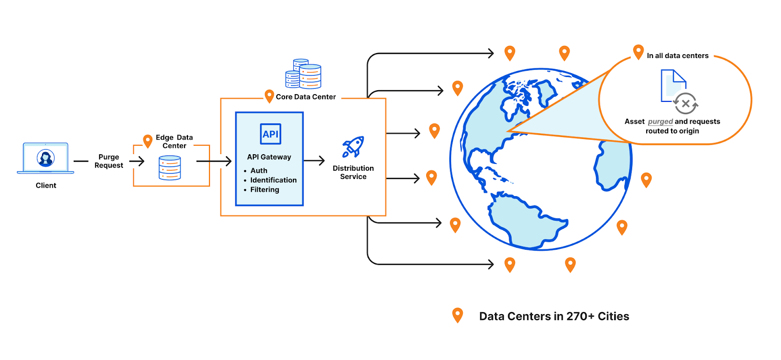
Core-based purge request entering a data center and getting backhauled to a core data center where Quicksilver distributes the request to all network data centers (hub and spoke).
Our first version of the flexible purge system used Quicksilver’s spoke-hub distribution to send purges from a core data center to every other data center in our network. It took less than a second for flexible purges to propagate, and once in a given data center, the purge key lookups in the hot path to force cache misses were in the low hundreds of microseconds. We were quite happy with this system at the time, especially because of the simplicity. Using well-supported internal infrastructure meant we weren’t having to manage database clusters or worry about transport between data centers ourselves, since we got that “for free”. Flexible purge was a new feature set and the performance seemed pretty good, especially since we had no predecessor to compare against.
Victims of our own success
Our first version of flexible purge didn’t start showing cracks for years, but eventually both our network and our customer base grew large enough that our system was reaching the limits of what it could scale to. As mentioned above, we needed to store purge requests beyond our maximum eviction age. Purge requests are relatively small, and compress well, but thousands of customers using the API millions of times a day adds up to quite a bit of storage that Quicksilver needed on each machine to maintain purge history, and all of that storage cut into disk space we could otherwise be using to cache customer content. We also found the limits of Quicksilver in terms of how many writes per second it could handle without replication slowing down. We bought ourselves more runway by putting Kafka queues in front of Quicksilver to buffer and throttle ourselves to even out traffic spikes, and increased batching, but all of those protections introduced latency. We knew we needed to come up with a solution without such a strong correlation between usage and operational costs.
Another pain point exposed by our growing user base that we mentioned in Part 2 was the excessive round trip times experienced by customers furthest away from our core data centers. A purge request sent by a customer in Australia would have to cross the Pacific Ocean and back before local customers would see the new content.
To summarize, three issues were plaguing us:
Latency corresponding to how far a customer was from the centralized ingest point.
Latency due to the bottleneck for writes at the centralized ingest point.
Storage needs in all data centers correlating strongly with throughput demand.
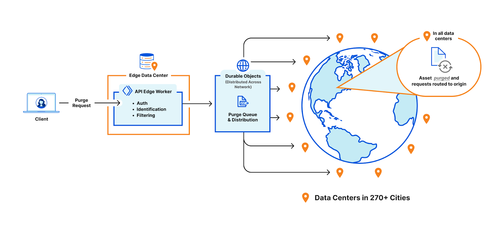
Coreless purge proves useful
The first two issues affected all types of purge. The spoke-hub distribution model was problematic for purge-by-URL just as much as it was for flexible purges. So we embarked on the path to peer-to-peer distribution for purge-by-URL to address the latency and throughput issues, and the results of that project were good enough that we wanted to propagate flexible purges through the same system. But doing so meant we’d have to replace our use of Quicksilver; it was so good at what it does (fast/reliable replication network-wide, extremely fast/high read throughput) in large part because of the core assumption of spoke-hub distribution it could optimize for. That meant there was no way to write to Quicksilver from “spoke” data centers, and we would need to find another storage system for our purges.
Flipping purge on its head
We decided if we’re going to replace our storage system we should dig into exactly what our needs are and find the best fit. It was time to revisit some of our oldest conclusions to see if they still held true, and one of the earlier ones was that proactively purging content from disk would be difficult to do efficiently given our storage layout.
But was that true? Or could we make active cache purge fast and efficient (enough)? What would it take to quickly find files on disk based on their metadata? “Indexes!” you’re probably screaming, and for good reason. Indexing files’ hostnames, cache-tags, and URLs would undoubtedly make querying for relevant files trivial, but a few aspects of our network make it less straightforward.
Cloudflare has hundreds of data centers that see trillions of unique files, so any kind of global index — even ignoring the networking hurdles of aggregation — would suffer the same type of bottlenecking issues with our previous spoke-hub system. Scoping the indices to the data center level would be better, but they vary in size up to several hundred machines. Managing a database cluster in each data center scaled to the appropriate size for the aggregate traffic of all the machines was a daunting proposition; it could easily end up being enough work on its own for a separate team, not something we should take on as a side hustle.
The next step down in scope was an index per machine. Indexing on the same machine as the cache proxy had some compelling upsides:
The proxy could talk to the index over UDS (Unix domain sockets), avoiding networking complexities in the hottest paths.
As a sidecar service, the index just had to be running anytime the machine was accepting traffic. If a machine died, so would the index, but that didn’t matter, so there wasn’t any need to deal with the complexities of distributed databases.
While data centers were frequently adding and removing machines, machines weren’t frequently adding and removing disks. An index could reasonably count on its maximum size being predictable and constant based on overall disk size.
But we wanted to make sure it was feasible on our machines. We analyzed representative cache disks from across our fleet, gathering data like the number of cached assets per terabyte and the average number of cache-tags per asset. We looked at cache MISS, REVALIDATED, and EXPIRED rates to estimate the required write throughput.
After conducting a thorough analysis, we were convinced the design would work. With a clearer understanding of the anticipated read/write throughput, we started looking at databases that could meet our needs. After benchmarking several relational and non-relational databases, we ultimately chose RocksDB, a high-performance embedded key-value store. We found that with proper tuning, it could be extremely good at the types of queries we needed.
Putting it all together
And so CacheDB was born — a service written in Rust and built on RocksDB, which operates on each machine alongside the cache proxy to manage the indexing and purging of cached files. We integrated the cache proxy with CacheDB to ensure that indices are stored whenever a file is cached or updated, and they’re deleted when a file is removed due to eviction or purging. In addition to indexing data, CacheDB maintains a local queue for buffering incoming purge operations. A background process reads purge operations in the queue, looking up all matching files using the indices, and deleting the matched files from disk. Once all matched files for an operation have been deleted, the process clears the indices and removes the purge operation from the queue.
To further optimize the speed of purges taking effect, the cache proxy was updated to check with CacheDB — similar to the previous lazy purge approach — when a cache HIT occurs before returning the asset. CacheDB does a quick scan of its local queue to see if there are any pending purge operations that match the asset in question, dictating whether the cache proxy should respond with the cached file or fetch a new copy. This means purges will prevent the cache proxy from returning a matching cached file as soon as a purge reaches the machine, even if there are millions of files that correspond to a purge key, and it takes a while to actually delete them all from disk.
Coreless purge using CacheDB and Durable Objects to distribute purges without needing to first stop at a core data center.
The last piece to change was the distribution pipeline, updated to broadcast flexible purges not just to every data center, but to the CacheDB service running on every machine. We opted for CacheDB to handle the last-mile fan out of machine to machine within a data center, using consul to keep each machine informed of the health of its peers. The choice let us keep the Workers largely the same for purge-by-URL (more here) and flexible purge handling, despite the difference in termination points.
The payoff
Our new approach reduced the long tail of the lazy purge, saving 10x storage. Better yet, we can now delete purged content immediately instead of waiting for the lazy purge to happen or expire. This new-found storage will improve cache retention on disk for all users, leading to improved cache HIT ratios and reduced egress from your origin.
The shift from lazy content purging (left) to the new Coreless Purge architecture allows us to actively delete content (right). This helps reduce storage needs and increase cache retention times across our service.
With the new coreless cache purge, we can now get a purge request into any datacenter, distribute the keys to purge, and instantly purge the content from the cache database. This all occurs in less than 150 milliseconds on P50 for tags, hostnames, and prefix URL, covering all 330 cities in 120+ countries.
Benchmarks
To measure Instant Purge, we wanted to make sure that we were looking at real user metrics — that these were purges customers were actually issuing and performance that was representative of what we were seeing under real conditions, rather than marketing numbers.
The time we measure represents the period when a request enters the local datacenter, and ends with when the purge has been executed in every datacenter. When the local data center receives the request, one of the first things we do is to add a timestamp to the purge request. When all data centers have completed the purge action, another timestamp is added to “stop the clock.” Each purge request generates this performance data, and it is then sent to a database for us to measure the appropriate quantiles and to help us understand how we can improve further.
In August 2024, we took purge performance data and segmented our collected data by region based on where the local data center receiving the request was located.
Region
P50 Aug 2024 (Coreless)
P50 May 2022 (Core-based)
Improvement
Africa
303ms
1,420ms
78.66%
Asia Pacific Region (APAC)
199ms
1,300ms
84.69%
Eastern Europe (EEUR)
140ms
1,240ms
88.70%
Eastern North America (ENAM)
119ms
1,080ms
88.98%
Oceania
191ms
1,160ms
83.53%
South America (SA)
196ms
1,250ms
84.32%
Western Europe (WEUR)
131ms
1,190ms
88.99%
Western North America (WNAM)
115ms
1,000ms
88.5%
Global
149ms
1,570ms
90.5%
Note: Global latency numbers on the core-based measurements (May 2022) may be larger than the regional numbers because it represents all of our data centers instead of only a regional portion, so outliers and retries might have an outsized effect.
What’s next?
We are currently wrapping up the roll-out of the last throughput changes which allow us to efficiently scale purge requests. As that happens, we will revise our rate limits and open up purge by tag, hostname, and prefix to all plan types! We expect to begin rolling out the additional purge types to all plans and users beginning in early 2025.
In addition, in the process of implementing this new approach, we have identified improvements that will shave a few more milliseconds off our single-file purge. Currently, single-file purges have a P50 of 234ms. However, we want to, and can, bring that number down to below 200ms.
If you want to come work on the world’s fastest purge system, check out our open positions.
Balancing developer velocity and security against bots is a constant challenge. Deploying your changes as quickly and easily as possible is essential to stay ahead of your (or your customers’) needs and wants. Ensuring your website is safe from malicious bots — without degrading user experience with alien hieroglyphics to decipher just to prove that you are a human — is no small feat. With Pages and Turnstile, we’ll walk you through just how easy it is to have the best of both worlds!
Cloudflare Pages offer a seamless platform for deploying and scaling your websites with ease. You can get started right away with configuring your websites with a quick integration using your git provider, and get set up with unlimited requests, bandwidth, collaborators, and projects.
Cloudflare Turnstile is Cloudflare’s CAPTCHA alternative solution where your users don’t ever have to solve another puzzle to get to your website, no more stop lights and fire hydrants. You can protect your site without having to put your users through an annoying user experience. If you are already using another CAPTCHA service, we have made it easy for you to migrate over to Turnstile with minimal effort needed. Check out the Turnstile documentation to get started.
Alright, what are we building?
In this tutorial, we’ll walk you through integrating Cloudflare Pages with Turnstile to secure your website against bots. You’ll learn how to deploy Pages, embed the Turnstile widget, validate the token on the server side, and monitor Turnstile analytics. Let’s build upon this tutorial from Cloudflare’s developer docs, which outlines how to create an HTML form with Pages and Functions. We’ll also show you how to secure it by integrating with Turnstile, complete with client-side rendering and server-side validation, using the Turnstile Pages Plugin!
Step 1: Deploy your Pages
On the Cloudflare Dashboard, select your account and go to Workers & Pages to create a new Pages application with your git provider. Choose the repository where you cloned the tutorial project or any other repository that you want to use for this walkthrough.
Once you select “Save and Deploy”, all the magic happens under the hood and voilà! The form is already deployed.
Step 2: Embed Turnstile widget
Now, let’s navigate to Turnstile and add the newly created Pages site.
Here are the widget configuration options:
Domain: All you need to do is add the domain for the Pages application. In this example, it’s “pages-turnstile-demo.pages.dev”. For each deployment, Pages generates a deployment specific preview subdomain. Turnstile covers all subdomains automatically, so your Turnstile widget will work as expected even in your previews. This is covered more extensively in our Turnstile domain management documentation.
Widget Mode: There are three types of widget modes you can choose from.
Managed: This is the recommended option where Cloudflare will decide when further validation through the checkbox interaction is required to confirm whether the user is a human or a bot. This is the mode we will be using in this tutorial.
Non-interactive: This mode does not require the user to interact and check the box of the widget. It is a non-intrusive mode where the widget is still visible to users but requires no added step in the user experience.
Invisible: Invisible mode is where the widget is not visible at all to users and runs in the background of your website.
Pre-Clearance setting: With a clearance cookie issued by the Turnstile widget, you can configure your website to verify every single request or once within a session. To learn more about implementing pre-clearance, check out this blog post.
Once you create your widget, you will be given a sitekey and a secret key. The sitekey is public and used to invoke the Turnstile widget on your site. The secret key should be stored safely for security purposes.
Let’s embed the widget above the Submit button. Your index.html should look like this:
<!doctype html>
<html lang="en">
<head>
<meta charset="utf8">
<title>Cloudflare Pages | Form Demo</title>
<meta name="theme-color" content="#d86300">
<meta name="mobile-web-app-capable" content="yes">
<meta name="apple-mobile-web-app-capable" content="yes">
<meta name="viewport" content="width=device-width,initial-scale=1">
<link rel="icon" type="image/png" href="https://www.cloudflare.com/favicon-128.png">
<link rel="stylesheet" href="/index.css">
<script src="https://challenges.cloudflare.com/turnstile/v0/api.js?onload=_turnstileCb" defer></script>
</head>
<body>
<main>
<h1>Demo: Form Submission</h1>
<blockquote>
<p>This is a demonstration of Cloudflare Pages with Turnstile.</p>
<p>Pages deployed a <code>/public</code> directory, containing a HTML document (this webpage) and a <code>/functions</code> directory, which contains the Cloudflare Workers code for the API endpoint this <code><form></code> references.</p>
<p><b>NOTE:</b> On form submission, the API endpoint responds with a JSON representation of the data. There is no JavaScript running in this example.</p>
</blockquote>
<form method="POST" action="/api/submit">
<div class="input">
<label for="name">Full Name</label>
<input id="name" name="name" type="text" />
</div>
<div class="input">
<label for="email">Email Address</label>
<input id="email" name="email" type="email" />
</div>
<div class="input">
<label for="referers">How did you hear about us?</label>
<select id="referers" name="referers">
<option hidden disabled selected value></option>
<option value="Facebook">Facebook</option>
<option value="Twitter">Twitter</option>
<option value="Google">Google</option>
<option value="Bing">Bing</option>
<option value="Friends">Friends</option>
</select>
</div>
<div class="checklist">
<label>What are your favorite movies?</label>
<ul>
<li>
<input id="m1" type="checkbox" name="movies" value="Space Jam" />
<label for="m1">Space Jam</label>
</li>
<li>
<input id="m2" type="checkbox" name="movies" value="Little Rascals" />
<label for="m2">Little Rascals</label>
</li>
<li>
<input id="m3" type="checkbox" name="movies" value="Frozen" />
<label for="m3">Frozen</label>
</li>
<li>
<input id="m4" type="checkbox" name="movies" value="Home Alone" />
<label for="m4">Home Alone</label>
</li>
</ul>
</div>
<div id="turnstile-widget" style="padding-top: 20px;"></div>
<button type="submit">Submit</button>
</form>
</main>
<script>
// This function is called when the Turnstile script is loaded and ready to be used.
// The function name matches the "onload=..." parameter.
function _turnstileCb() {
console.debug('_turnstileCb called');
turnstile.render('#turnstile-widget', {
sitekey: '0xAAAAAAAAAXAAAAAAAAAAAA',
theme: 'light',
});
}
</script>
</body>
</html>
You can embed the Turnstile widget implicitly or explicitly. In this tutorial, we will explicitly embed the widget by injecting the JavaScript tag and related code, then specifying the placement of the widget.
Make sure that the div id you assign is the same as the id you specify in turnstile.render call. In this case, let’s use “turnstile-widget”. Once that’s done, you should see the widget show up on your site!
Now that the Turnstile widget is rendered on the front end, let’s validate it on the server side and check out the Turnstile outcome. We need to make a call to the /siteverify API with the token in the submit function under ./functions/api/submit.js.
First, grab the token issued from Turnstile under cf-turnstile-response. Then, call the /siteverify API to ensure that the token is valid. In this tutorial, we’ll attach the Turnstile outcome to the response to verify everything is working well. You can decide on the expected behavior and where to direct the user based on the /siteverify response.
/**
 * POST /api/submit
 */

import turnstilePlugin from "@cloudflare/pages-plugin-turnstile";

// This is a demo secret key. In prod, we recommend you store
// your secret key(s) safely.
const SECRET_KEY = '0x4AAAAAAASh4E5cwHGsTTePnwcPbnFru6Y';

export const onRequestPost = [
    turnstilePlugin({
    	secret: SECRET_KEY,
    }),
    (async (context) => {
    	// Request has been validated as coming from a human
    	const formData = await context.request.formData()

    	var tmp, outcome = {};
	for (let [key, value] of formData) {
		tmp = outcome[key];
		if (tmp === undefined) {
			outcome[key] = value;
		} else {
			outcome[key] = [].concat(tmp, value);
		}
	}

	// Attach Turnstile outcome to the response
	outcome["turnstile_outcome"] = context.data.turnstile;

	let pretty = JSON.stringify(outcome, null, 2);

      	return new Response(pretty, {
      		headers: {
      			'Content-Type': 'application/json;charset=utf-8'
      		}
      	});
    })
];
Since Turnstile accurately decided that the visitor was not a bot, the response for “success” is “true” and “interactive” is “false”. The “interactive” being “false” means that the checkbox was automatically checked by Cloudflare as the visitor was determined to be human. The user was seamlessly allowed access to the website without having to perform any additional actions. If the visitor looks suspicious, Turnstile will become interactive, requiring the visitor to actually click the checkbox to verify that they are not a bot. We used the managed mode in this tutorial but depending on your application logic, you can choose the widget mode that works best for you.
Now that we’ve set up Turnstile, we can head to Turnstile analytics in the Cloudflare Dashboard to monitor the solve rate and widget traffic. Visitor Solve Rate indicates the percentage of visitors who successfully completed the Turnstile widget. A sudden drop in the Visitor Solve Rate could indicate an increase in bot traffic, as bots may fail to complete the challenge presented by the widget. API Solve Rate measures the percentage of visitors who successfully validated their token against the /siteverify API. Similar to the Visitor Solve Rate, a significant drop in the API Solve Rate may indicate an increase in bot activity, as bots may fail to validate their tokens. Widget Traffic provides insights into the nature of the traffic hitting your website. A high number of challenges requiring interaction may suggest that bots are attempting to access your site, while a high number of unsolved challenges could indicate that the Turnstile widget is effectively blocking suspicious traffic.
And that’s it! We’ve walked you through how to easily secure your Pages with Turnstile. Pages and Turnstile are currently available for free for every Cloudflare user to get started right away. If you are looking for a seamless and speedy developer experience to get a secure website up and running, protected by Turnstile, head over to the Cloudflare Dashboard today!
For years, we’ve written that CAPTCHAs drive us crazy. Humans give up on CAPTCHA puzzles approximately 15% of the time and, maddeningly, CAPTCHAs are significantly easier for bots to solve than they are for humans. We’ve spent the past three and a half years working to build a better experience for humans that’s just as effective at stopping bots. As of this month, we’ve finished replacing every CAPTCHA issued by Cloudflare withTurnstile, our new CAPTCHA replacement (pictured below). Cloudflare will never issue another visual puzzle to anyone, for any reason.
Now that we’ve eliminated CAPTCHAs at Cloudflare, we want to make it easy for anyone to do the same, even if they don’t use other Cloudflare services. We’ve decoupled Turnstile from our platform so that any website operator on any platform can use it just by adding a few lines of code. We’re thrilled to announce that Turnstile is now generally available, and Turnstile’s ‘Managed’ mode is now completely free to everyone for unlimited use.
Easy on humans, hard on bots, private for everyone
There’s a lot that goes into Turnstile’s simple checkbox to ensure that it’s easy for everyone, preserves user privacy, and does its job stopping bots. Part of making challenges better for everyone means that everyone gets the same great experience, no matter what browser you’re using. Because we do not employ a visual puzzle, users with low vision or blindness get the same easy to use challenge flow as everyone else. It was particularly important for us to avoid falling back to audio CAPTCHAs to offer an experience accessible to everyone. Audio CAPTCHAs are often much worse than even visual CAPTCHAs for humans to solve, with only 31.2% of audio challenges resulting in a three-person agreement on what the correct solution actually is. The prevalence of free speech-to-text services has made it easy for bots to solve audio CAPTCHAs as well, with a recent study showing bots can accurately solve audio CAPTCHAs in over 85% of attempts.
We also created Turnstile to be privacy focused. Turnstile meets ePrivacy Directive, GDPR and CCPA compliance requirements, as well as the strict requirements of our own privacy commitments. In addition, Cloudflare's FedRAMP Moderate authorized package, "Cloudflare for Government" now includes Turnstile. We don’t rely on tracking user data, like what other websites someone has visited, to determine if a user is a human or robot. Our business is protecting websites, not selling ads, so operators can deploy Turnstile knowing that their users’ data is safe.
With all of our emphasis on how easy it is to pass a Turnstile challenge, you would be right to ask how it can stop a bot. If a bot can find all images with crosswalks in grainy photos faster than we can, surely it can check a box as well. Bots definitely can check a box, and they can even mimic the erratic path of human mouse movement while doing so. For Turnstile, the actual act of checking a box isn’t important, it’s the background data we’re analyzing while the box is checked that matters. We find and stop bots by running a series of in-browser tests, checking browser characteristics, native browser APIs, and asking the browser to pass lightweight tests (ex: proof-of-work tests, proof-of-space tests) to prove that it’s an actual browser. The current deployment of Turnstile checks billions of visitors every day, and we are able to identify browser abnormalities that bots exhibit while attempting to pass those tests.
For over one year, we used our Managed Challenge to rotate between CAPTCHAs and our own Turnstile challenge to compare our effectiveness. We found that even without asking users for any interactivity at all, Turnstile was just as effective as a CAPTCHA. Once we were sure that the results were effective at coping with the response from bot makers, we replaced the CAPTCHA challenge with our own checkbox solution. We present this extra test when we see potentially suspicious signals, and it helps us provide an even greater layer of security.
Turnstile is great for fighting fraud
Like all sites that offer services for free, Cloudflare sees our fair share of automated account signups, which can include “new account fraud,” where bad actors automate the creation of many different accounts to abuse our platform. To help combat this abuse, we’ve rolled out Turnstile’s invisible mode to protect our own signup page. This month, we’ve blocked over1 million automated signup attempts using Turnstile, without a reported false positive or any change in our self-service billings that rely on this signup flow.
Lessons from the Turnstile beta
Over the past twelve months, we’ve been grateful to see how many people are eager to try, then rely on, and integrate Turnstile into their web applications. It’s been rewarding to see the developer community embrace Turnstile as well. We list some of the community created Turnstile integrations here, including integrations with WordPress, Angular, Vue, and a Cloudflare recommended React library. We’ve listened to customer feedback, and added support for 17 new languages, new callbacks, and new error codes.
76,000+ users have signed up, but our biggest single test by far was the Eurovision final vote. Turnstile runs on challenge pages on over 25 million Cloudflare websites. Usually, that makes Cloudflare the far and away biggest Turnstile consumer, until the final Eurovision vote. During that one hour, challenge traffic from the Eurovision voting site outpaced the use of challenge pages on those 25 million sites combined! Turnstile handled the enormous spike in traffic without a hitch.
While a lot went well during the Turnstile beta, we also encountered some opportunities for us to learn. We were initially resistant to disclosing why a Turnstile challenge failed. After all, if bad actors know what we’re looking for, it becomes easier for bots to fool our challenges until we introduce new detections. However, during the Turnstile beta, we saw a few scenarios where legitimate users could not pass a challenge. These scenarios made it clear to us that we need to be transparent about why a challenge failed to help aid any individual who might modify their browser in a way that causes them to get caught by Turnstile. We now publish detailed client-side error codes to surface the reason why a challenge has failed. Two scenarios came up on several occasions that we didn’t expect:
First, we saw that desktop computers at least 10 years old frequently had expired motherboard batteries, and computers with bad motherboard batteries very often keep inaccurate time. This is because without the motherboard battery, a desktop computer’s clock will stop operating when the computer is off. Turnstile checks your computer’s system time to detect when a website operator has accidentally configured a challenge page to be cached, as caching a challenge page will cause it to become impassable. Unfortunately, this same check was unintentionally catching humans who just needed to update the time. When we see this issue, we now surface a clear error message to the end user to update their system time. We’d prefer to never have to surface an error in the first place, so we’re working to develop new ways to check for cached content that won’t impact real people.
Second, we find that a few privacy-focused users often ask their browsers to go beyond standard practices to preserve their anonymity. This includes changing their user-agent (something bots will do to evade detection as well), and preventing third-party scripts from executing entirely. Issues caused by this behavior can now be displayed clearly in a Turnstile widget, so those users can immediately understand the issue and make a conscientious choice about whether they want to allow their browser to pass a challenge.
Although we have some of the most sensitive, thoroughly built monitoring systems at Cloudflare, we did not catch either of these issues on our own. We needed to talk to users affected by the issue to help us understand what the problem was. Going forward, we want to make sure we always have that direct line of communication open. We’re rolling out a new feedback form in the Turnstile widget, to ensure any future corner cases are addressed quickly and with urgency.
Turnstile: GA and Free for Everyone
Announcing Turnstile’s General Availability means that Turnstile is now completely production ready, available for free for unlimited use via our visible widget in Managed mode. Turnstile Enterprise includes SaaS platform support and a visible mode without the Cloudflare logo. Self-serve customers can expect a pay-as-you-go option for advanced features to be available in early 2024. Users can continue to access Turnstile’s advanced features below our 1 million siteverify request limit, as has been the case during the beta. If you’ve been waiting to try Turnstile, head over to our signup page and create an account!
This blog reports and summarizes the contents of a Cloudflare research paper which appeared at the ACM Internet Measurement Conference, that measures and prototypes connection coalescing with ORIGIN Frames.
Some readers might be surprised to hear that a single visit to a web page can cause a browser to make tens, sometimes even hundreds, of web connections. Take this very blog as an example. If it is your first visit to the Cloudflare blog, or it has been a while since your last visit, your browser will make multiple connections to render the page. The browser will make DNS queries to find IP addresses corresponding to blog.cloudflare.com and then subsequent requests to retrieve any necessary subresources on the web page needed to successfully render the complete page. How many? Looking below, at the time of writing, there are 32 different hostnames used to load the Cloudflare Blog. That means 32 DNS queries and at least 32 TCP (or QUIC) connections, unless the client is able to reuse (or coalesce) some of those connections.
Each new web connection not only introduces additional load on a server's processing capabilities – potentially leading to scalability challenges during peak usage hours – but also exposes client metadata to the network, such as the plaintext hostnames being accessed by an individual. Such meta information can potentially reveal a user’s online activities and browsing behaviors to on-path network adversaries and eavesdroppers!
In this blog we’re going to take a closer look at “connection coalescing”. Since our initial look at IP-based coalescing in 2021, we have done further large-scale measurements and modeling across the Internet, to understand and predict if and where coalescing would work best. Since IP coalescing is difficult to manage at large scale, last year we implemented and experimented with a promising standard called the HTTP/2 ORIGIN Frame extension that we leveraged to coalesce connections to our edge without worrying about managing IP addresses.
All told, there are opportunities being missed by many large providers. We hope that this blog (and our publication at ACM IMC 2022 with full details) offers a first step that helps servers and clients take advantage of the ORIGIN Frame standard.
Setting the stage
At a high level, as a user navigates the web, the browser renders web pages by retrieving dependent subresources to construct the complete web page. This process bears a striking resemblance to the way physical products are assembled in a factory. In this sense, a modern web page can be considered like an assembly plant. It relies on a ‘supply chain’ of resources that are needed to produce the final product.
An assembly plant in the physical world can place a single order for different parts and get a single shipment from the supplier (similar to the kitting process for maximizing value and minimizing response time); no matter the manufacturer of those parts or where they are made — one ‘connection’ to the supplier is all that is needed. Any single truck from a supplier to an assembly plant can be filled with parts from multiple manufacturers.
The design of the web causes browsers to typically do the opposite in nature. To retrieve the images, JavaScript, and other resources on a web page (the parts), web clients (assembly plants) have to make at least one connection to every hostname (the manufacturers) defined in the HTML that is returned by the server (the supplier). It makes no difference if the connections to those hostnames go to the same server or not, for example they could go to a reverse proxy like Cloudflare. For each manufacturer a ‘new’ truck would be needed to transfer the materials to the assembly plant from the same supplier, or more formally, a new connection would need to be made to request a subresource from a hostname on the same web page.
Without connection coalescing
The number of connections used to load a web page can be surprisingly high. It is also common for the subresources to need yet other sub-subresources, and so new connections emerge as a result of earlier ones. Remember, too, that HTTP connections to hostnames are often preceded by DNS queries! Connection coalescing allows us to use fewer connections, or ‘reuse’ the same set of trucks to carry parts from multiple manufacturers from a single supplier.
With connection coalescing
Connection coalescing in principle
Connection coalescing was introduced in HTTP/2, and carried over into HTTP/3. We’ve blogged about connection coalescing previously (for a detailed primer we encourage going over that blog). While the idea is simple, implementing it can present a number of engineering challenges. For example, recall from above that there are 32 hostnames (at the time of writing) to load the web page you are reading right now. Among the 32 hostnames are 16 unique domains (defined as “Effective TLD+1”). Can we create fewer connections or ‘coalesce’ existing connections for each unique domain? The answer is ‘Yes, but it depends’.
The exact number of connections to load the blog page is not at all obvious, and hard to know. There may be 32 hostnames attached to 16 domains but, counter-intuitively, this does not mean the answer to “how many unique connections?” is 16. The true answer could be as few as one connection if all the hostnames are reachable at a single server; or as many as 32 independent connections if a different and distinct server is needed to access each individual hostname.
Connection reuse comes in many forms, so it’s important to define “connection coalescing” in the HTTP space. For example, the reuse of an existing TCP or TLS connection to a hostname to make multiple requests for subresources from that same hostname is connection reuse, but not coalescing.
Coalescing occurs when an existing TLS channel for some hostname can be repurposed or used for connecting to a different hostname. For example, upon visiting blog.cloudflare.com, the HTML points to subresources at cdnjs.cloudflare.com. To reuse the same TLS connection for the subresources, it is necessary for both hostnames to appear together in the TLS certificate's “Server Alternative Name (SAN)” list, but this step alone is not sufficient to convince browsers to coalesce. After all, the cdnjs.cloudflare.com service may or may not be reachable at the same server as blog.cloudflare.com, despite being on the same certificate. So how can the browser know? Coalescing only works if servers set up the right conditions, but clients have to decide whether to coalesce or not – thus, browsers require a signal to coalesce beyond the SANs list on the certificate. Revisiting our analogy, the assembly plant may order a part from a manufacturer directly, not knowing that the supplier already has the same part in its warehouse.
There are two explicit signals a browser can use to decide whether connections can be coalesced: one is IP-based, the other ORIGIN Frame-based. The former requires the server operators to tightly bind DNS records to the HTTP resources available on the server. This is difficult to manage and deploy, and actually creates a risky dependency, because you have to place all the resources behind a specific set or a single IP address. The way IP addresses influence coalescing decisions varies among browsers, with some choosing to be more conservative and others more permissive. Alternatively, the HTTP ORIGIN Frame is an easier signal for the servers to orchestrate; it’s also flexible and has graceful failure with no interruption to service (for a specification compliant implementation).
A foundational difference between both these coalescing signals is: IP-based coalescing signals are implicit, even accidental, and force clients to infer coalescing possibilities that may exist, or not. None of this is surprising since IP addresses are designed to have no real relationship with names! In contrast, ORIGIN Frame is an explicit signal from servers to clients that coalescing is available no matter what DNS says for any particular hostname.
We have experimented with IP-based coalescing previously; for the purpose of this blog we will take a deeper look at ORIGIN Frame-based coalescing.
What is the ORIGIN Frame standard?
The ORIGIN Frame is an extension to the HTTP/2 and HTTP/3 specification, a special Frame sent on stream 0 or the control stream of the connection respectively. The Frame allows the servers to send an ‘origin-set’ to the clients on an existing established TLS connection, which includes hostnames that it is authorized for and will not incur any HTTP 421 errors. Hostnames in the origin-set MUST also appear in the certificate SAN list for the server, even if those hostnames are announced on different IP addresses via DNS.
Specifically, two different steps are required:
Web servers must send a list enumerating the Origin Set (the hostnames that a given connection might be used for) in the ORIGIN Frame extension.
The TLS certificate returned by the web server must cover the additional hostnames being returned in the ORIGIN Frame in the DNS names SAN entries.
At a high-level ORIGIN Frames are a supplement to the TLS certificate that operators can attach to say, “Psst! Hey, client, here are the names in the SANs that are available on this connection — you can coalesce!” Since the ORIGIN Frame is not part of the certificate itself, its contents can be made to change independently. No new certificate is required. There is also no dependency on IP addresses. For a coalesceable hostname, existing TCP/QUIC+TLS connections can be reused without requiring new connections or DNS queries.
Many websites today rely on content which is served by CDNs, like Cloudflare CDN service. The practice of using external CDN services offers websites the advantages of speed, reliability, and reduces the load of content served by their origin servers. When both the website, and the resources are served by the same CDN, despite being different hostnames, owned by different entities, it opens up some very interesting opportunities for CDN operators to allow connections to be reused and coalesced since they can control both the certificate management and connection requests for sending ORIGIN frames on behalf of the real origin server.
Unfortunately, there has been no way to turn the possibilities enabled by ORIGIN Frame into practice. To the best of our knowledge, until today, there has been no server implementation that supports ORIGIN Frames. Among browsers, only Firefox supports ORIGIN Frames. Since IP coalescing is challenging and ORIGIN Frame has no deployed support, is the engineering time and energy to better support coalescing worth the investment? We decided to find out with a large-scale Internet-wide measurement to understand the opportunities and predict the possibilities, and then implemented the ORIGIN Frame to experiment on production traffic.
Experiment #1: What is the scale of required changes?
In February 2021, we collected data for 500K of the most popular websites on the Internet, using a modified Web Page Test on 100 virtual machines. An automated Chrome (v88) browser instance was launched for every visit to a web page to eliminate caching effects (because we wanted to understand coalescing, not caching). On successful completion of each session, Chrome developer tools were used to retrieve and write the page load data as an HTTP Archive format (HAR) file with a full timeline of events, as well as additional information about certificates and their validation. Additionally, we parsed the certificate chains for the root web page and new TLS connections triggered by subresource requests to (i) identify certificate issuers for the hostnames, (ii) inspect the presence of the Subject Alternative Name (SAN) extension, and (iii) validate that DNS names resolve to the IP address used. Further details about our methodology and results can be found in the technical paper.
The first step was to understand what resources are requested by web pages to successfully render the page contents, and where these resources were present on the Internet. Connection coalescing becomes possible when subresource domains are ideally co-located. We approximated the location of a domain by finding its corresponding autonomous system (AS). For example, the domain attached to cdnjs is reachable via AS 13335 in the BGP routing table, and that AS number belongs to Cloudflare. The figure below describes the percentage of web pages and the number of unique ASes needed to fully load a web page.
Around 14% of the web pages need two ASes to fully load i.e. pages that have a dependency on one additional AS for subresources. More than 50% of the web pages need to contact no more than six ASes to obtain all the necessary subresources. This finding as shown in the plot above implies that a relatively small number of operators serve the sub-resource content necessary for a majority (~50%) of the websites, and any usage of ORIGIN Frames would need only a few changes to have its intended impact. The potential for connection coalescing can therefore be optimistically approximated to the number of unique ASes needed to retrieve all subresources in a web page. In practice however, this may be superseded by operational factors such as SLAs or helped by flexible mappings between sockets, names, and IP addresses which we worked on previously at Cloudflare.
We then tried to understand the impact of coalescing on connection metrics. The measured and ideal number of DNS queries and TLS connections needed to load a web page are summarized by their CDFs in the figure below.
Through modeling and extensive analysis, we identify that connection coalescing through ORIGIN Frames could reduce the number of DNS and TLS connections made by browsers by over 60% at the median. We performed this modeling by identifying the number of times the clients requested DNS records, and combined them with the ideal ORIGIN Frames to serve.
Many multi-origin servers such as those operated by CDNs tend to reuse certificates and serve the same certificate with multiple DNS SAN entries. This allows the operators to manage fewer certificates through their creation and renewal cycles. While theoretically one can have millions of names in the certificate, creating such certificates is unreasonable and a challenge to manage effectively. By continuing to rely on existing certificates, our modeling measurements bring to light the volume of changes required to enable perfect coalescing, while presenting information about the scale of changes needed, as highlighted in the figure below.
We identify that over 60% of the certificates served by websites do not need any modifications and could benefit from ORIGIN Frames, while with no more than 10 additions to the DNS SAN names in certificates we’re able to successfully coalesce connections to over 92% of the websites in our measurement. The most effective changes could be made by CDN providers by adding three or four of their most popular requested hostnames into each certificate.
Experiment #2: ORIGIN Frames in action
In order to validate our modeling expectations, we then took a more active approach in early 2022. Our next experiment focused on 5,000 websites that make extensive use of cdnjs.cloudflare.com as a subresource. By modifying our experimental TLS termination endpoint we deployed HTTP/2 ORIGIN Frame support as defined in the RFC standard. This involved changing the internal fork of net and http dependency modules of Golang which we have open sourced (see here, and here).
During the experiments, connecting to a website in the experiment set would return cdnjs.cloudflare.com in the ORIGIN frame, while the control set returned an arbitrary (unused) hostname. All existing edge certificates for the 5000 websites were also modified. For the experimental group, the corresponding certificates were renewed with cdnjs.cloudflare.com added to the SAN. To ensure integrity between control and experimental sets, control group domains certificates were also renewed with a valid and identical size third party domain used by none of the control domains. This is done to ensure that the relative size changes to the certificates is kept constant avoiding potential biases due to different certificate sizes. Our results were striking!
Sampling 1% of the requests we received from Firefox to the websites in the experiment, we identified over 50% reduction in new TLS connections per second indicating a lesser number of cryptographic verification operations done by both the client and reduced server compute overheads. As expected there were no differences in the control set indicating the effectiveness of connection re-use as seen by the CDN or server operators.
Discussion and insights
While our modeling measurements indicated that we could anticipate some performance improvements, in practice it was not significantly better suggesting that ‘no-worse’ is the appropriate mental model regarding performance. The subtle interplay between resource object sizes, competing connections, and congestion control is subject to network conditions. Bottleneck-share capacity, for example, diminishes as fewer connections compete for bottleneck resources on network links. It would be interesting to revisit these measurements as more operators deploy support on their servers for ORIGIN Frames.
Apart from performance, one major benefit of ORIGIN frames is in terms of privacy. How? Well, each coalesced connection hides client metadata that is otherwise leaked from non-coalesced connections. Certain resources on a web page are loaded depending on how one is interacting with the website. This means for every new connection for retrieving some resource from the server, TLS plaintext metadata like SNI (in the absence of Encrypted Client Hello) and at least one plaintext DNS query, if transmitted over UDP or TCP on port 53, is exposed to the network. Coalescing connections helps remove the need for browsers to open new TLS connections, and the need to do extra DNS queries. This prevents metadata leakage from anyone listening on the network. ORIGIN Frames help minimize those signals from the network path, improving privacy by reducing the amount of cleartext information leaked on path to network eavesdroppers.
While the browsers benefit from reduced cryptographic computations needed to verify multiple certificates, a major advantage comes from the fact that it opens up very interesting future opportunities for resource scheduling at the endpoints (the browsers, and the origin servers) such as prioritization, or recent proposals like HTTP early hints to provide clients experiences where connections are not overloaded or competing for those resources. When coupled with CERTIFICATE Frames IETF draft, we can further eliminate the need for manual certificate modifications as a server can prove its authority of hostnames after connection establishment without any additional SAN entries on the website’s TLS certificate.
Conclusion and call to action
In summary, the current Internet ecosystem has a lot of opportunities for connection coalescing with only a few changes to certificates and their server infrastructure. Servers can significantly reduce the number of TLS handshakes by roughly 50%, while reducing the number of render blocking DNS queries by over 60%. Clients additionally reap these benefits in privacy by reducing cleartext DNS exposure to network on-lookers.
To help make this a reality we are currently planning to add support for both HTTP/2 and HTTP/3 ORIGIN Frames for our customers. We also encourage other operators that manage third party resources to adopt support of ORIGIN Frame to improve the Internet ecosystem. Our paper submission was accepted to the ACM Internet Measurement Conference 2022 and is available for download. If you’d like to work on projects like this, where you get to see the rubber meet the road for new standards, visit our careers page!
In January 2021, we gave you a behind-the-scenes look at how we built Waiting Room on Cloudflare’s Durable Objects. Today, we are thrilled to announce the launch of Waiting Room Analytics and tell you more about how we built this feature. Waiting Room Analytics offers insights into end-user experience and provides visualizations of your waiting room traffic. These new metrics enable you to make well-informed configuration decisions, ensuring an optimal end-user experience while protecting your site from overwhelming traffic spikes.
If you’ve ever bought tickets for a popular concert online you’ll likely have been put in a virtual queue. That’s what Waiting Room provides. It keeps your site up and running in the face of overwhelming traffic surges. Waiting Room sends excess visitors to a customizable virtual waiting room and admits them to your site as spots become available.
While customers have come to rely on the protection Waiting Room provides against traffic surges, they have faced challenges analyzing their waiting room’s performance and impact on end-user flow. Without feedback about waiting room traffic as it relates to waiting room settings, it was challenging to make Waiting Room configuration decisions.
Up until now, customers could only monitor their waiting room's status endpoint to get a general idea of waiting room traffic. This endpoint displays the current number of queued users, active users on the site, and the estimated wait time shown to the last user in line.
The status endpoint is still a great tool for at a glance understanding of the near real-time status of a waiting room. However, there were many questions customers had about their waiting room that were either difficult or impossible to answer using the status endpoint, such as:
How long did visitors wait in the queue?
What was my peak number of visitors?
How long was the pre-queue for my online event?
How did changing my waiting room's settings impact wait times?
Today, Waiting Room is ready to answer those questions and more with the launch of Waiting Room Analytics, available in the Waiting Room dashboard to all Business and Enterprise plans! We will show you the new waiting room metrics available and review how these metrics can help you make informed decisions about your waiting room's settings. We'll also walk you through the unique challenge of how we built Waiting Room Analytics on our distributed network.
How Waiting Room settings impact traffic
Before covering the newly available Waiting Room metrics, let's review some key settings you configure when creating a waiting room. Understanding these settings is essential as they directly impact your waiting room's analytics, traffic, and user experience.
When configuring a waiting room, you will first define traffic limits to your site by setting two values–Total active users and New users per minute. Total active users is a target threshold for how many simultaneous users you want to allow on the pages covered by your waiting room. Waiting Room will kick in as traffic ramps up to keep active users near this limit. The other value which will control the volume of traffic allowed past your waiting room is New users per minute. This setting defines the target threshold for the maximum rate of user influx to your application. Waiting Room will kick in when the influx accelerates to keep this rate near your limits. Queuing occurs when traffic is at or near your New users per minute or Total active users target values.
The two other settings which will impact your traffic flow and user wait times are Session duration and session renewal. The session duration setting determines how long it takes for end-user sessions to expire, thereby freeing up spots on your site. If you enable session renewal, users can stay on your site as long as they want, provided they make a request once every session_duration minutes. If you disable session renewal, users' sessions will expire after the duration you set for session_duration has run out. After the session expires, the user will be issued a new waiting room cookie upon their next request. If there is active queueing, this user will be placed in the back of the queue. Otherwise, they can continue browsing for another session_duration minutes.
Let's walk through the new analytics available in the Waiting Room dashboard, which allows you to see how these settings can impact waiting room throughput, how many users get queued, and how long users wait to enter your site from the queue.
Waiting Room Analytics in the dash
To access metrics for a waiting room, navigate to the Waiting Room dashboard, where you can find pre-built visualizations of your waiting room traffic. The dashboard offers at-a-glance metrics for the peak waiting room traffic over the last 24 hours.
To dig deeper and analyze up to 30 days of historical data, open your waiting room's analytics by selecting View more.
Alternatively, we've made it easy to hone in on analytics for a past waiting room event (within the last 30 days). You can automatically open the analytics dashboard to a past event's exact start and end time, including the pre-queueing period by selecting the blue link in the events table.
User insights
The first two metrics–Time in queue and Time on origin–provide insights into your end-users' experience and behavior. The time in queue values help you understand how long queued users waited before accessing your site over the time period selected. The time on origin values shed light on end-user behavior by displaying an estimate of the range of time users spend on your site before leaving. If session renewal is disabled, this time will max out at session_duration and reflect the time at which users are issued a new waiting room cookie. For both metrics, we provide time for both the typical user, represented by a range of the 50th and 75th percentile of users, as well as for the top 5% of users who spend the longest in the queue or on your site.
If session renewal is disabled, keeping an eye on Time on origin values is especially important. When sessions do not renew, once a user's session has expired, they are given a new waiting room cookie upon their next request. The user will be put at the back of the line if there is active queueing. Otherwise, they will continue browsing, but their session timer will start over and your analytics will never show a Time on origin greater than your configured session duration, even if individual users are on your site longer than the session duration. If session renewal is disabled and the typical time on origin is close to your configured session duration, this could be an indicator you may need to give your users more time to complete their journey before putting them back in line.
Analyze past waiting room traffic
Scrolling down the page, you will find visualizations of your user traffic compared to your waiting room's target thresholds for Total active users and New users per minute. These two settings determine when your waiting room will start queueing as traffic increases. The Total active users setting controls the number of concurrent users on your site, while the New users per minute threshold restricts the flow rate of users onto your site.
To zoom in on a time period, you can drag your cursor from the left to the right of the time period you are interested in and the other graphs, in addition to the insights will update to reflect this time period.
On the Active users graph, each bar represents the maximum number of queued users stacked on top of the maximum number of users on your site at that point in time. The example below shows how the waiting room kicked in at different times with respect to the active user threshold. The total length of the bar illustrates how many total users were either on the site or waiting to enter the site at that point in time, with a clear divide between those two values where the active user threshold kicked in. Hover over any bar to display a tooltip with the exact values for the period you are interested in.
Easily identify peak traffic and when waiting room started queuing to protect your site from a traffic surge.
Below the Active users chart is the New users per minute graph, which shows the rate of users entering your application per minute compared to your configured threshold. Make sure to review this graph to identify any surges in the rate of users to your application that may have caused queueing.
The New users per minute graph helps you identify peaks in the rate of users entering your site which triggered queueing.This graph shows queued user and active user data from the same time period as the spike seen in New users per minute graph above. When analyzing your waiting room’s metrics, be sure to review both graphs to understand which Waiting Room traffic setting triggered queueing and to what extent.
Adjusting settings with Waiting Room Analytics
By leveraging the insights provided by the analytics dashboard, you can fine-tune your waiting room settings while ensuring a safe and seamless user experience. A common concern for customers is longer than desired wait times during high traffic periods. We will walk through some guidelines for evaluating peak traffic and settings’ adjustments that could be made.
Identify peak traffic. The first step is to identify when peak traffic occurred. To do so, zoom out to 30 days or some time period inclusive of a known high traffic event. Reviewing the graph, locate a period of time where traffic peaked and use your cursor to highlight from the left to right of the peak. This will zoom in to that time period, updating all other values on the analytics page.
Evaluate wait times. Now that you have honed in on the time period of peak traffic, review the Time in queue metric to analyze if the wait times during peak traffic were acceptable. If you determine that wait times were significantly longer than you had anticipated, consider the following options to reduce wait times for your next traffic peak.
Decrease session duration when session renewal is enabled. This is a safe option as it does not increase the allowed load to your site. By decreasing this duration, you decrease the amount of time it takes for spots to open up as users go idle. This is a good option if your customer journey is typically request heavy, such as a checkout flow. For other situations, such as video streaming or long-form content viewing, this may not be a good option as users may not make frequent requests even though they are not actually idle.
Disable session renewal. This option also does not increase the allowed load to your site. Disabling session renewal means that users will have session_duration minutes to stay on the site before being put back in the queue. This option is popular for high demand events such as product drops, where customers want to give as many users as possible a fair chance to participate and avoid inventory hoarding. When disabling session renewal, review your waiting room’s analytics to determine an appropriate session duration to set.
The Time on origin values will give you an idea of how long users need before leaving your site. In the example below, the session duration is set to 10 minutes but even the users who spend the longest only spend around 5 minutes on the site. With the session renewal disabled, this customer could reduce wait times by decreasing the session duration to 5 minutes without disruption to most users, allowing for more users to get access.
Adjust Total active users or New users per minute settings. Lastly, you can decrease wait times by increasing your waiting room’s traffic limits–Total active users or New users per minute. This is the most sure-fire way to reduce wait times but it also requires more consideration. Before increasing either limit, you will need to evaluate if it is safe to do so and make small, iterative adjustments to these limits, monitoring certain signals to ensure your origin is still able to handle the load. A few things to consider monitoring as you adjust settings are origin CPU usage and memory utilization, and increases in 5xx errors which can be reviewed in Cloudflare’s Web Analytics tab. Analyze historical traffic patterns during similar events or periods of high demand. If you observe that previous traffic surges were successfully managed without site instability or crashes, it provides a strong signal that you can consider increasing waiting room limits.
Utilize the Active user chart as well as the New users per minute chart to determine which limit is primarily responsible for triggering queuing so that you know which limit to adjust. After considering these signals and making adjustments to your waiting room’s traffic limits, closely monitor the impact of these changes using the waiting room analytics dashboard. Continuously assess the performance and stability of your site, keeping an eye on server metrics and user feedback.
How we built Waiting Room Analytics
At Cloudflare, we love to build on top of our own products. Waiting Room is built on Workers and Durable Objects. Workers have the ability to auto-scale based on the request rate. They are built using isolates enabling them to spin up hundreds or thousands of isolates within 5 milliseconds without much overhead. Every request that goes to an application behind a waiting room, goes to a Worker.
We optimized the way in which we track end users visiting the application while maintaining their position in the queue. Tracking every user individually would incur more overhead in terms of maintaining state, consuming more CPU & memory. Instead, we decided to divide the users into buckets based on the timestamp of the first request made by the end user. For example, all the users who visited a waiting room between 00:00:00 and 00:00:59 for the first time are assigned to the bucket 00:00:00. Every end user gets a unique encrypted cookie on the first request to the waiting room. The contents of the cookie keep getting updated based on the status of the users in the queue. Once the end user is accepted to the origin, we set the cookie expiry to session_duration minutes, which can be set in the dashboard, from the last request timestamp. In the cookie we track the timestamp of when the end user joined the queue which is used in the calculation of time waited in queue.
Collection of metrics in a distributed environment
a
In a distributed environment, the challenge when building out analytics is to collect data from multiple nodes and aggregate them. Each worker running at every data center sees user requests and needs to report metrics based on those to another coordinating service at every data center. The data aggregation could have been done in two ways.
i) Writing data from every worker when a request is received In this design, every worker that receives a request is responsible for reporting the metrics. This would enable us to write the raw data to our analytics pipeline. We would not have the overhead of aggregating the data before writing. This would mean that we would write data for every request, but Waiting Room configurations are minute based and every user is put into a bucket based on the timestamp of the first request. All our configurations are minute and user based and the data written from workers is not related to time or user.
ii) Using the existing aggregation pipeline Waiting Room is designed in such a way that we do not track every request, instead we group users into buckets based on the first time we saw them. This is tracked in the cookie that is issued to the user when they make the first request. In the current system, the data reported by the workers is sent upstream to the data center coordinator which is responsible for aggregating the data seen from all the workers for that particular data center. This aggregated data is then further processed and sent upstream to the global Durable Object which aggregates the data from all the other data centers. This data is used for making decisions whether to queue the user or to send them to the origin.
We decided to use the existing pipeline that is used for Waiting Room routing for analytics. Data aggregated this way provides more value to customers as it matches the model we use for routing decisions. Therefore, customers can see directly how changing their settings affects waiting room behavior. Also, it is an optimization in terms of space. Instead of writing analytics data per request, we are writing a pre-processed and aggregated analytics log every minute. This way the data is much less noisy.
This diagram depicts that multiple workers from different locations receive requests and talk to the data center coordinators respectively which aggregate data and report the aggregated keys upstream to the Global Durable Object. The Global Durable Objects further aggregate all the keys received from the data center coordinators to compute a global aggregate key.
Histograms
The metrics available via Cloudflare’s GraphQL API are a combination of configured values set by the customer when creating a waiting room and values that are computed based on traffic seen by a waiting room. Waiting Room aggregates data every minute for each metric based on the requests it sees. While some metrics like new users per minute, total active users are counts and can be pre-processed and aggregated with a simple summation, metrics like time on origin and total time waited in queue cannot simply be added together into a single metric.
For example, there could be users who waited in the queue for four minutes and there could be a new user who joined the queue two minutes ago. However, if we simply sum these two data points, it would not make sense because six minutes would be an incorrect representation of the total time waited in the queue. Therefore, to capture this value more accurately, we store the data in a histogram. This enables us to represent the typical case (50th percentile) and the approximate worst case (in this case 95th percentile) for that metric.
Intuitively, we decided to store time on origin and total time waited in queue into a histogram distribution so that we would be able to represent the data and calculate quantiles precisely. We used Hdr Histogram – A High Dynamic Range Histogram for recording the data in histograms. Hdr Histograms are scalable and we were able to record dynamic numbers of values with auto-resizing without inflating CPU, memory or introducing latency. The time to record a value in the Hdr Histograms range from 3-6 nanoseconds. Querying and recording values can be done in constant time. Two histogram data structures can simply be added together into a bigger histogram. Also, the histograms can be compressed and encoded/decoded into base64 strings. This enabled us to scalably pass the data structure within our internal services for further aggregation.
The memory footprint of hdr histograms is constant and depends on the size of the bucket, precision and range of the histogram. The size of the bucket we use is the default 32 bits bucket size. The precision of the histogram is set to include up to three significant digits. The histogram has a dynamic range of values enabled through the use of the auto-resize functionality. However, to ensure efficient data storage, a limit of 5,000 recorded points per minute has been imposed. Although this limit was chosen arbitrarily, it has proven to be adequate for storing data points transmitted from the workers to the Durable Objects on a minute-by-minute basis.
The requests to the website behind a Waiting Room go to a Cloudflare data center that is close to their location. Our workers from around the world record values in the histogram which is compressed and sent to the data center Durable Object periodically. The histograms from multiple workers are uncompressed and aggregated into a single histogram per data center. The resulting histogram is compressed and sent upstream to the Global Durable objects where the histograms from all data centers receiving traffic are uncompressed and aggregated. The resulting histogram is the final data structure which is used for statistical analysis. We directly query the aggregated histogram for the quantile values. The histogram objects were instantiated once at the start of the service, they were reset after every successful sync with the upstream service.
Writing data to the pipeline
The global Durable Object aggregates all the metrics, computes quantiles and sends the data to a worker which is responsible for analytics reporting. This worker reads data from Workers KV in order to get the Waiting Room configurations. All the metrics are aggregated into a single analytics message. These messages are written every minute to Clickhouse. We leveraged an internal version of Workers Analytics Engine in order to write the data. This allowed us to quickly write our logs to Clickhouse with minimum interactions with all the systems involved in the pipeline.
We write analytics events from the runtime in the form of blobs and doubles with a specific schema and the event data gets written to a Clickhouse cluster. We extract the data into a Clickhouse view and apply ABR to facilitate fast queries at any timescale. You can expand the time range to vary from 30 minutes to 30 days without any lag. ABR adaptively chooses the resolution of data based on the query. For example, it would choose a lower resolution for a long time range and vice versa. As of now, the analytics data is available in the Clickhouse table for 30 days, implying that you can not query data older than 30 days in the dashboard as well.
Sampling
Waiting Room Analytics samples the data in order to effectively run large queries while providing consistent response times. Indexing the data on Waiting Room id has enabled us to run quicker and more efficient scans, however we still need to elegantly handle unbounded data. To tackle this we use Adaptive Bit Rate which enables us to write the data at multiple resolutions (100%, 10%, 1%…) and then read the best resolution of the data. The sample rate “adapts” based on how long the query takes to run. If the query takes too long to run in 100% resolution, the next resolution is picked and so on until the first successful result. However, since we pre-process and aggregate data before writing to the pipeline, we expect 100% resolution of data on reads for shorter periods of time (up to 7 days). For a longer time range, the data will be sampled.
Get Waiting Room Analytics via GraphQL API
Lastly, to make metrics available to customers and to the Waiting Room dashboard, we exposed the analytics data available in Clickhouse via GraphQL API.
If you prefer to build your own dashboards or systems based on waiting room traffic data, then Waiting Room Analytics via GraphQL API is for you. Build your own custom dashboards using the GraphQL framework and use a GraphQL client such as GraphiQL to run queries and explore the schema.
The Waiting Room Analytics dataset can be found under the Zones Viewer as waitingRoomAnalyticsAdaptive and waitingRoomAnalyticsAdaptiveGroups. You can filter the dataset per zone, waiting_room_id and the request time period, see the dataset schema under ZoneWaitingRoomAnalyticsAdaptive. You can order the data by ascending or descending order of the metric values.
You can explore the dimensions under waitingRoomAnalyticsAdaptiveGroups that can be used to group the data based on time, Waiting Room id and so on. The "max", “min”, “avg”, “sum” functions give the maximum, minimum, average and sum values of a metric aggregated over a time period. Additionally, there is a function called "avgWeighted" that calculates the weighted average of the metric. This approach is used for metrics stored in histograms, such as the time spent on the origin and total time waited. Instead of using a simple average, the weighted average is computed to provide a more accurate representation. This approach takes into account the distribution and significance of different data points, ensuring a more precise analysis and interpretation of the metric.
For example, to evaluate the weighted average for time spent on origin, the value of total active users is used as a weight. To better illustrate this concept, let’s consider an example. Imagine there is a website behind a Waiting Room and we want to evaluate the average time spent on the origin over a certain time period, let’s say an hour. During this hour, the number of active users on the website fluctuates. At some points, there may be more users actively browsing the site while at other times the number of active users might decrease. To calculate the weighted average for the time spent on the origin, we take into account the number of total active users at each instant in time. The rationale behind this is that the more users are actively using the website, the more representative their time spent on origin becomes in relation to the overall user activity.
By incorporating the total active users as weights in the calculation, we give more importance to the time spent on the origin during periods when there are more users actively engaging with the website. This provides a more accurate representation of the average time spent on the origin, accounting for variations in user activity throughout the designated time period.
The value of new users per minute is used as a weight to compute the weighted average for total time waited in queue. This is because when we talk about the total time weighted in the queue, the value of new users per minute for that instant in time takes importance as it signifies the number of users that joined the queue and certainly went into the origin.
You can apply these aggregation functions to the list of metrics exposed under each function. However, if you just want the logs per minute for a time period, rather than the breakdown of the time period (minute, fifteen minutes, hours), you can remove the datetime dimension from the query. For a list of sample queries to get you started, refer to our dev docs.
Below is a query to calculate the average, maximum and minimum of total active users, estimated wait time, total queued users and session duration every fifteen minutes. It also calculates the weighted average of time spent in queue and time spent on origin. The query is done on the zone level. The response is obtained in a JSON format.
Following is an example query to find the weighted averages of time on origin (50th percentile) and total time waited (90th percentile) for a certain period and aggregate this data over one hour.
You can find more examples in our developer documentation. Waiting Room Analytics is live and available to all Business and Enterprise customers and we are excited for you to explore it! Don’t have a waiting room set up? Make sure your site is always protected from unexpected traffic surges. Try out Waiting Room today!
Our previous post reviewed usage trends for HTTP/1.1, HTTP/2, and HTTP/3 observed across Cloudflare’s network between May 2021 and May 2022, broken out by version and browser family, as well as for search engine indexing and social media bots. At the time, we found that browser-driven traffic was overwhelmingly using HTTP/2, although HTTP/3 usage was showing signs of growth. Search and social bots were mixed in terms of preference for HTTP/1.1 vs. HTTP/2, with little-to-no HTTP/3 usage seen.
Between May 2022 and May 2023, we found that HTTP/3 usage in browser-retrieved content continued to grow, but that search engine indexing and social media bots continued to effectively ignore the latest version of the web’s core protocol. (Having said that, the benefits of HTTP/3 are very user-centric, and arguably offer minimal benefits to bots designed to asynchronously crawl and index content. This may be a key reason that we see such low adoption across these automated user agents.) In addition, HTTP/3 usage across API traffic is still low, but doubled across the year. Support for HTTP/3 is on by default for zones using Cloudflare’s free tier of service, while paid customers have the option to activate support.
HTTP/1.1 and HTTP/2 use TCP as a transport layer and add security via TLS. HTTP/3 uses QUIC to provide both the transport layer and security. Due to the difference in transport layer, user agents usually require learning that an origin is accessible using HTTP/3 before they'll try it. One method of discovery is HTTP Alternative Services, where servers return an Alt-Svc response header containing a list of supported Application-Layer Protocol Negotiation Identifiers (ALPN IDs). Another method is the HTTPS record type, where clients query the DNS to learn the supported ALPN IDs. The ALPN ID for HTTP/3 is "h3" but while the specification was in development and iteration, we added a suffix to identify the particular draft version e.g., "h3-29" identified draft 29. In order to maintain compatibility for a wide range of clients, Cloudflare advertised both "h3" and "h3-29". However, draft 29 was published close to three years ago and clients have caught up with support for the final RFC. As of late May 2023, Cloudflare no longer advertises h3-29 for zones that have HTTP/3 enabled, helping to save several bytes on each HTTP response or DNS record that would have included it. Because a browser and web server typically automatically negotiate the highest HTTP version available, HTTP/3 takes precedence over HTTP/2.
In the sections below, “likely automated” and “automated” traffic based on Cloudflare bot score has been filtered out for desktop and mobile browser analysis to restrict analysis to “likely human” traffic, but it is included for the search engine and social media bot analysis. In addition, references to HTTP requests or HTTP traffic below include requests made over both HTTP and HTTPS.
Overall request distribution by HTTP version
Aggregating global web traffic to Cloudflare on a daily basis, we can observe usage trends for HTTP/1.1, HTTP/2, and HTTP/3 across the surveyed one year period. The share of traffic over HTTP/1.1 declined from 8% to 7% between May and the end of September, but grew rapidly to over 11% through October. It stayed elevated into the new year and through January, dropping back down to 9% by May 2023. Interestingly, the weekday/weekend traffic pattern became more pronounced after the October increase, and remained for the subsequent six months. HTTP/2 request share saw nominal change over the year, beginning around 68% in May 2022, but then starting to decline slightly in June. After that, its share didn’t see a significant amount of change, ending the period just shy of 64%. No clear weekday/weekend pattern was visible for HTTP/2. Starting with just over 23% share in May 2022, the percentage of requests over HTTP/3 grew to just over 30% by August and into September, but dropped to around 26% by November. After some nominal loss and growth, it ended the surveyed time period at 28% share. (Note that this graph begins in late May due to data retention limitations encountered when generating the graph in early June.)
API request distribution by HTTP version
Although API traffic makes up a significant amount of Cloudflare’s request volume, only a small fraction of those requests are made over HTTP/3. Approximately half of such requests are made over HTTP/1.1, with another third over HTTP/2. However, HTTP/3 usage for APIs grew from around 6% in May 2022 to over 12% by May 2023. HTTP/3’s smaller share of traffic is likely due in part to support for HTTP/3 in key tools like curl still being considered as “experimental”. Should this change in the future, with HTTP/3 gaining first-class support in such tools, we expect that this will accelerate growth in HTTP/3 usage, both for APIs and overall as well.
Mitigated request distribution by HTTP version
The analyses presented above consider all HTTP requests made to Cloudflare, but we also thought that it would be interesting to look at HTTP version usage by potentially malicious traffic, so we broke out just those requests that were mitigated by one of Cloudflare’s application security solutions. The graph above shows that the vast majority of mitigated requests are made over HTTP/1.1 and HTTP/2, with generally less than 5% made over HTTP/3. Mitigated requests appear to be most frequently made over HTTP/1.1, although HTTP/2 accounted for a larger share between early August and late November. These observations suggest that attackers don’t appear to be investing the effort to upgrade their tools to take advantage of the newest version of HTTP, finding the older versions of the protocol sufficient for their needs. (Note that this graph begins in late May 2022 due to data retention limitations encountered when generating the graph in early June 2023.)
HTTP/3 use by desktop browser
As we noted last year, support for HTTP/3 in the stable release channels of major browsers came in November 2020 for Google Chrome and Microsoft Edge, and April 2021 for Mozilla Firefox. We also noted that in Apple Safari, HTTP/3 support needed to be enabled in the “Experimental Features” developer menu in production releases. However, in the most recent releases of Safari, it appears that this step is no longer necessary, and that HTTP/3 is now natively supported.
Looking at request shares by browser, Chrome started the period responsible for approximately 80% of HTTP/3 request volume, but the continued growth of Safari dropped it to around 74% by May 2023. A year ago, Safari represented less than 1% of HTTP/3 traffic on Cloudflare, but grew to nearly 7% by May 2023, likely as a result of support graduating from experimental to production.
Removing Chrome from the graph again makes trends across the other browsers more visible. As noted above, Safari experienced significant growth over the last year, while Edge saw a bump from just under 10% to just over 11% in June 2022. It stayed around that level through the new year, and then gradually dropped below 10% over the next several months. Firefox dropped slightly, from around 10% to just under 9%, while reported HTTP/3 traffic from Internet Explorer was near zero.
As we did in last year’s post, we also wanted to look at how the share of HTTP versions has changed over the last year across each of the leading browsers. The relative stability of HTTP/2 and HTTP/3 seen over the last year is in some contrast to the observations made in last year’s post, which saw some noticeable shifts during the May 2021 – May 2022 timeframe.
In looking at request share by protocol version across the major desktop browser families, we see that across all of them, HTTP/1.1 share grows in late October. Further analysis indicates that this growth was due to significantly higher HTTP/1.1 request volume across several large customer zones, but it isn’t clear why this influx of traffic using an older version of HTTP occurred. It is clear that HTTP/2 remains the dominant protocol used for content requests by the major browsers, consistently accounting for 50-55% of request volume for Chrome and Edge, and ~60% for Firefox. However, for Safari, HTTP/2’s share dropped from nearly 95% in May 2022 to around 75% a year later, thanks to the growth in HTTP/3 usage.
HTTP/3 share on Safari grew from under 3% to nearly 18% over the course of the year, while its share on the other browsers was more consistent, with Chrome and Edge hovering around 40% and Firefox around 35%, and both showing pronounced weekday/weekend traffic patterns. (That pattern is arguably the most pronounced for Edge.) Such a pattern becomes more, yet still barely, evident with Safari in late 2022, although it tends to vary by less than a percent.
HTTP/3 usage by mobile browser
Mobile devices are responsible for over half of request volume to Cloudflare, with Chrome Mobile generating more than 25% of all requests, and Mobile Safari more than 10%. Given this, we decided to explore HTTP/3 usage across these two key mobile platforms.
Looking at Chrome Mobile and Chrome Mobile Webview (an embeddable version of Chrome that applications can use to display Web content), we find HTTP/1.1 usage to be minimal, topping out at under 5% of requests. HTTP/2 usage dropped from 60% to just under 55% between May and mid-September, but then bumped back up to near 60%, remaining essentially flat to slightly lower through the rest of the period. In a complementary fashion, HTTP/3 traffic increased from 37% to 45%, before falling just below 40% in mid-September, hovering there through May. The usage patterns ultimately look very similar to those seen with desktop Chrome, albeit without the latter’s clear weekday/weekend traffic pattern.
Perhaps unsurprisingly, the usage patterns for Mobile Safari and Mobile Safari Webview closely mirror those seen with desktop Safari. HTTP/1.1 share increases in October, and HTTP/3 sees strong growth, from under 3% to nearly 18%.
Search indexing bots
Exploring usage of the various versions of HTTP by search engine crawlers/bots, we find that last year’s trend continues, and that there remains little-to-no usage of HTTP/3. (As mentioned above, this is somewhat expected, as HTTP/3 is optimized for browser use cases.) Graphs for Bing & Baidu here are trimmed to a period ending April 1, 2023 due to anomalous data during April that is being investigated.
GoogleBot continues to rely primarily on HTTP/1.1, which generally comprises 55-60% of request volume. The balance is nearly all HTTP/2, although some nominal growth in HTTP/3 usage sees it peaking at just under 2% in March.
Through January 2023, around 85% of requests from Microsoft’s BingBot were made via HTTP/2, but dropped to closer to 80% in late January. The balance of the requests were made via HTTP/1.1, as HTTP/3 usage was negligible.
Looking at indexing bots from search engines based outside of the United States, Russia’s YandexBot appears to use HTTP/1.1 almost exclusively, with HTTP/2 usage generally around 1%, although there was a period of increased usage between late August and mid-November. It isn’t clear what ultimately caused this increase. There was no meaningful request volume seen over HTTP/3. The indexing bot used by Chinese search engine Baidu also appears to strongly prefer HTTP/1.1, generally used for over 85% of requests. However, the percentage of requests over HTTP/2 saw a number of spikes, briefly reaching over 60% on days in July, November, and December 2022, as well as January 2023, with several additional spikes in the 30% range. Again, it isn’t clear what caused this spiky behavior. HTTP/3 usage by BaiduBot is effectively non-existent as well.
Social media bots
Similar to Bing & Baidu above, the graphs below are also trimmed to a period ending April 1.
Facebook’s use of HTTP/3 for site crawling and indexing over the last year remained near zero, similar to what we observed over the previous year. HTTP/1.1 started the period accounting for under 60% of requests, and except for a brief peak above it in late May, usage of HTTP/1.1 steadily declined over the course of the year, dropping to around 30% by April 2023. As such, use of HTTP/2 increased from just over 40% in May 2022 to over 70% in April 2023. Meta engineers confirmed that this shift away from HTTP/1.1 usage is an expected gradual change in their infrastructure's use of HTTP, and that they are slowly working towards removing HTTP/1.1 from their infrastructure entirely.
In last year’s blog post, we noted that “TwitterBot clearly has a strong and consistent preference for HTTP/2, accounting for 75-80% of its requests, with the balance over HTTP/1.1.” This preference generally remained the case through early October, at which point HTTP/2 usage began a gradual decline to just above 60% by April 2023. It isn’t clear what drove the week-long HTTP/2 drop and HTTP/1.1 spike in late May 2022. And as we noted last year, TwitterBot’s use of HTTP/3 remains non-existent.
In contrast to Facebook’s and Twitter’s site crawling bots, HTTP/3 actually accounts for a noticeable, and growing, volume of requests made by LinkedIn’s bot, increasing from just under 1% in May 2022 to just over 10% in April 2023. We noted last year that LinkedIn’s use of HTTP/2 began to take off in March 2022, growing to approximately 5% of requests. Usage of this version gradually increased over this year’s surveyed period to 15%, although the growth was particularly erratic and spiky, as opposed to a smooth, consistent increase. HTTP/1.1 remained the dominant protocol used by LinkedIn’s bots, although its share dropped from around 95% in May 2022 to 75% in April 2023.
Conclusion
On the whole, we are excited to see that usage of HTTP/3 has generally increased for browser-based consumption of traffic, and recognize that there is opportunity for significant further growth if and when it starts to be used more actively for API interactions through production support in key tools like curl. And though disappointed to see that search engine and social media bot usage of HTTP/3 remains minimal to non-existent, we also recognize that the real-time benefits of using the newest version of the web’s foundational protocol may not be completely applicable for asynchronous automated content retrieval.
This was a weekend of record-breaking DDoS attacks. Over the weekend, Cloudflare detected and mitigated dozens of hyper-volumetric DDoS attacks. The majority of attacks peaked in the ballpark of 50-70 million requests per second (rps) with the largest exceeding 71 million rps. This is the largest reported HTTP DDoS attack on record, more than 35% higher than the previous reported record of 46M rps in June 2022.
The attacks were HTTP/2-based and targeted websites protected by Cloudflare. They originated from over 30,000 IP addresses. Some of the attacked websites included a popular gaming provider, cryptocurrency companies, hosting providers, and cloud computing platforms. The attacks originated from numerous cloud providers, and we have been working with them to crack down on the botnet.
Record breaking attack: DDoS attack exceeding 71 million requests per second
Over the past year, we’ve seen more attacks originate from cloud computing providers. For this reason, we will be providing service providers that own their own autonomous system a free Botnet threat feed. The feed will provide service providers threat intelligence about their own IP space; attacks originating from within their autonomous system. Service providers that operate their own IP space can now sign up to the early access waiting list.
Is this related to the Super Bowl or Killnet?
No. This campaign of attacks arrives less than two weeks after the Killnet DDoS campaign that targeted healthcare websites. Based on the methods and targets, we do not believe that these recent attacks are related to the healthcare campaign. Furthermore, yesterday was the US Super Bowl, and we also do not believe that this attack campaign is related to the game event.
What are DDoS attacks?
Distributed Denial of Service attacks are cyber attacks that aim to take down Internet properties and make them unavailable for users. These types of cyberattacks can be very efficient against unprotected websites and they can be very inexpensive for the attackers to execute.
An HTTP DDoS attack usually involves a flood of HTTP requests towards the target website. The attacker’s objective is to bombard the website with more requests than it can handle. Given a sufficiently high amount of requests, the website’s server will not be able to process all of the attack requests along with the legitimate user requests. Users will experience this as website-load delays, timeouts, and eventually not being able to connect to their desired websites at all.
Illustration of a DDoS attack
To make attacks larger and more complicated, attackers usually leverage a network of bots — a botnet. The attacker will orchestrate the botnet to bombard the victim’s websites with HTTP requests. A sufficiently large and powerful botnet can generate very large attacks as we’ve seen in this case.
However, building and operating botnets requires a lot of investment and expertise. What is the average Joe to do? Well, an average Joe that wants to launch a DDoS attack against a website doesn’t need to start from scratch. They can hire one of numerous DDoS-as-a-Service platforms for as little as $30 per month. The more you pay, the larger and longer of an attack you’re going to get.
Why DDoS attacks?
Over the years, it has become easier, cheaper, and more accessible for attackers and attackers-for-hire to launch DDoS attacks. But as easy as it has become for the attackers, we want to make sure that it is even easier – and free – for defenders of organizations of all sizes to protect themselves against DDoS attacks of all types.
Unlike Ransomware attacks, Ransom DDoS attacks don’t require an actual system intrusion or a foothold within the targeted network. Usually Ransomware attacks start once an employee naively clicks an email link that installs and propagates the malware. There’s no need for that with DDoS attacks. They are more like a hit-and-run attack. All a DDoS attacker needs to know is the website’s address and/or IP address.
Is there an increase in DDoS attacks?
Yes. The size, sophistication, and frequency of attacks has been increasing over the past months. In our latest DDoS threat report, we saw that the amount of HTTP DDoS attacks increased by 79% year-over-year. Furthermore, the amount of volumetric attacks exceeding 100 Gbps grew by 67% quarter-over-quarter (QoQ), and the number of attacks lasting more than three hours increased by 87% QoQ.
But it doesn’t end there. The audacity of attackers has been increasing as well. In our latest DDoS threat report, we saw that Ransom DDoS attacks steadily increased throughout the year. They peaked in November 2022 where one out of every four surveyed customers reported being subject to Ransom DDoS attacks or threats.
Distribution of Ransom DDoS attacks by month
Should I be worried about DDoS attacks?
Yes. If your website, server, or networks are not protected against volumetric DDoS attacks using a cloud service that provides automatic detection and mitigation, we really recommend that you consider it.
Cloudflare customers shouldn’t be worried, but should be aware and prepared. Below is a list of recommended steps to ensure your security posture is optimized.
What steps should I take to defend against DDoS attacks?
Cloudflare’s systems have been automatically detecting and mitigating these DDoS attacks.
Cloudflare offers many features and capabilities that you may already have access to but may not be using. So as extra precaution, we recommend taking advantage of these capabilities to improve and optimize your security posture:
Ensure all DDoS Managed Rules are set to default settings (High sensitivity level and mitigation actions) for optimal DDoS activation.
Cloudflare Enterprise customers that are subscribed to the Advanced DDoS Protection service should consider enabling Adaptive DDoS Protection, which mitigates attacks more intelligently based on your unique traffic patterns.
Deploy firewall rules and rate limiting rules to enforce a combined positive and negative security model. Reduce the traffic allowed to your website based on your known usage.
Ensure your origin is not exposed to the public Internet (i.e., only enable access to Cloudflare IP addresses). As an extra security precaution, we recommend contacting your hosting provider and requesting new origin server IPs if they have been targeted directly in the past.
Customers with access to Managed IP Lists should consider leveraging those lists in firewall rules. Customers with Bot Management should consider leveraging the threat scores within the firewall rules.
Enable caching as much as possible to reduce the strain on your origin servers, and when using Workers, avoid overwhelming your origin server with more subrequests than necessary.
Defending against DDoS attacks is critical for organizations of all sizes. While attacks may be initiated by humans, they are executed by bots — and to play to win, you must fight bots with bots. Detection and mitigation must be automated as much as possible, because relying solely on humans to mitigate in real time puts defenders at a disadvantage. Cloudflare’s automated systems constantly detect and mitigate DDoS attacks for our customers, so they don’t have to. This automated approach, combined with our wide breadth of security capabilities, lets customers tailor the protection to their needs.
We’ve been providing unmetered and unlimited DDoS protection for free to all of our customers since 2017, when we pioneered the concept. Cloudflare’s mission is to help build a better Internet. A better Internet is one that is more secure, faster, and reliable for everyone – even in the face of DDoS attacks.
You’re visiting your family for the holidays and you connect to the WiFi, and then notice Netflix isn’t loading as fast as it normally does. You go to speed.cloudflare.com, fast.com, speedtest.net, or type “speed test” into Google Chrome to figure out if there is a problem with your Internet connection, and get something that looks like this:
If you want to see what that looks like for you, try it yourself here. But what do those numbers mean? How do those numbers relate to whether or not your Netflix isn’t loading or any of the other common use cases: playing games or audio/video chat with your friends and loved ones? Even network engineers find that speed tests are difficult to relate to the user experience of… using the Internet..
Amazingly, speed tests have barely changed in nearly two decades, even though the way we use the Internet has changed a lot. With so many more people on the Internet, the gaps between speed tests and the user’s experience of network quality are growing. The problem is so important that the Internet’s standards organization is paying attention, too.
From a high-level, there are three grand network test challenges:
Finding ways to efficiently and accurately measure network quality, and convey to end-users if and how the quality affects their experience.
When a problem is found, figuring out where the problem exists, be it the wireless connection, or one many cables and machines that make up the Internet.
Understanding a single user’s test results in context of their neighbors’, or archiving the results to, for example, compare neighborhoods or know if the network is getting better or worse.
Cloudflare is excited to announce a new Aggregated Internet Measurement (AIM) initiative to help address all three challenges. AIM is a new and open format for displaying Internet quality in a way that makes sense to end users of the Internet, around use cases that demand specific types of Internet performance while still retaining all of the network data engineers need to troubleshoot problems on the Internet. We’re excited to partner with Measurement Lab on this project and store all of this data in a publicly available repository that you can access to analyze the data behind the scores you see on your speed test page.
What is a speed test?
A speed test is a point-in-time measurement of your Internet connection. When you connect to any speed test, it typically tries to fetch a large file (important for video streaming), performs a packet loss test (important for gaming), measures jitter (important for video/VoIP calls), and latency (important for all Internet use cases). The goal of this test is to measure your Internet connection’s ability to perform basic tasks.
There are some challenges with this approach that start with a simple observation: At the “network-layer” of the Internet that moves data and packets around, there are three and only three measures that can be directly observed. They are,
available bandwidth, sometimes known as “throughput;
packet loss, which has to happen but not too much; and
latency, often referred to as the round-trip time (RTT).
These three attributes are tightly interwoven. In particular, the portion of available bandwidth that a user actually achieves (throughput) is directly affected by loss and latency. Your computer uses loss and latency to decide when to send a packet, or not. Some loss and latency is expected, even needed! Too much of either, and bandwidth starts to fall.
These are simple numbers, but their relationship is far from simple. Think about all the ways to add two numbers to equal as much as one-hundred, x + y ≤ 100. If x and y are just right, then they add to one hundred. However, there are many combinations of x and y that do. Worse is that if either x or y or both are a little wrong, then they add to less than one-hundred. In this example, x and y are loss and latency, and 100 is the available bandwidth.
There are other forces at work, too, and these numbers do not tell the whole story. But they are the only numbers that are directly observable. Their meaning and the reasons they matter for diagnosis are important, so let’s discuss each one of those in order and how Aggregated Internet Measurement tries to solve each of these.
What do the numbers in a speed test mean?
Most speed tests will run and produce the numbers you saw above: bandwidth, latency, jitter, and packet loss. Let’s break down each of these numbers one by one to explain what they mean:
Bandwidth
Bandwidth is the maximum throughput/capacity over a communication link. The common analogy used to define bandwidth is if your Internet connection is a highway, bandwidth is how many lanes the highway has and cars that fit on it. Bandwidth has often been called “speed” in the past because Internet Service Providers (ISPs) measure speed as the amount of time it takes to download a large file, and having more bandwidth on your connection can make that happen faster.
Packet loss
Packet loss is exactly what it sounds like: some packets are sent from a source to a destination, but the packets are not received by the destination. This can be very impactful for many applications, because if information is lost in transit en route to the receiver, it an e ifiult fr te recvr t udrsnd wt s bng snt (it can be difficult for the receiver to understand what is being sent).
Latency
Latency is the time it takes for a packet/message to travel from point A to point B. At its core, the Internet is composed of computers sending signals in the form of electrical signals or beams of light over cables to other computers. Latency has generally been defined as the time it takes for that electrical signal to go from one computer to another over a cable or fiber. Therefore, it follows that one way to reduce latency is to shrink the distance the signals need to travel to reach their destination.
There is a distinction in latency between idle latency and latency under load. This is because there are queues at routers and switches that store data packets when they arrive faster than they can be transmitted. Queuing is normal, by design, and keeps data flowing correctly. However, if the queues are too big, or when other applications behave very differently from yours, the connection can feel slower than it actually is. This event is called bufferbloat.
In our AIM test we look at idle latency to show you what your latency could be, but we also collect loaded latency, which is a better reflection of what your latency is during your day-to-day Internet experience.
Jitter
Jitter is a special way of measuring latency. It is the variance in latency on your Internet connection. If jitter is high, it may take longer for some packets to arrive, which can impact Internet scenarios that require content to be delivered in real time, such as voice communication.
A good way to think about jitter is to think about a commute to work along some route or path. Latency, alone, asks “how far am I from the destination measured in time?” For example, the average journey on a train is 40 minutes. Instead of journey time, jitter asks, “how consistent is my travel time?” Thinking about the commute, a jitter of zero means the train always takes 40 minutes. However, if the jitter is 15 then, well, the commute becomes a lot more challenging because it could take anywhere from 25 to 55 minutes.
But even if we understand these numbers, for all that they might tell us what is happening, they are unable to tell us where something is happening.
Is Wi-Fi or my Internet connection the problem?
When you run a speed test, you’re not just connecting to your ISP, you’re also connecting to your local network which connects to your ISP. And your local network may have problems of its own. Take a speed test that has high packet loss and jitter: that generally means something on the network could be dropping packets. Normally, you would call your ISP, who will often say something like “get closer to your Wi-Fi access point or get an extender”.
This is important — Wi-Fi uses radio waves to transmit information, and materials like brick, plaster, and concrete can interfere with the signal and make it weaker the farther away you get from your access point. Mesh Wi-Fi appliances like Nest Wi-Fi and Eero periodically take speed tests from their main access point specifically to help detect issues like this. So having potential quick solutions for problems like high packet loss and jitter and giving that to users up front can help users better ascertain if the problem is related to their wireless connection setup.
While this is true for most issues that we see on the Internet, it often helps if network operators are able to look at this data in aggregate in addition to simply telling users to get closer to their access points. If your speed test went to a place where your network operator could see it and others in your area, network engineers may be able to proactively detect issues before users report them. This not only helps users, it helps network providers as well, because fielding calls and sending out technicians for issues due to user configuration are expensive in addition to being time-consuming.
This is one of the goals of AIM: to help solve the problem before anyone picks up a phone. End users can get a series of tips that will help them understand what their Internet connection can and can’t do and how they can improve it in an easy-to-read format, and network operators can get all the data they need to detect last mile issues before anyone picks up a phone, saving time and money. Let’s talk about how that can work with a real example.
An example from real life
When you get a speed test result, the numbers you get can be confusing. This is because you may not understand how those numbers combine to impact your Internet experience. Let’s talk about a real life example and how that impacts you.
Say you work in a building with four offices and a main area that looks like this:
You have to make video calls to your clients all day, and you sit in the office the farthest away from the wireless access point. Your calls are dropping constantly, and you’re having an awful experience. When you run a speed test from your office, you see this result:
Metric
Far away from access point
Close to access point
Download Bandwidth
21.8 Mbps
25.7 Mbps
Upload Bandwidth
5.66 Mbps
5.26 Mbps
Unloaded Latency
19.6 ms
19.5 ms
Jitter
61.4 ms
37.9 ms
Packet Loss
7.7%
0%
How can you make sense of these? A network engineer would take a look at the high jitter and the packet loss and think “well this user probably needs to move closer to the router to get a better signal”. But you may take a look at these results and have no idea, and have to ask a network engineer for help, which could lead to a call to your ISP, wasting the time and money of everyone. But you shouldn’t have to consult a network engineer to figure out if you need to move your Wi-Fi access point, or if your ISP isn’t giving her a good experience.
Aggregated Internet Measurement assigns qualitative assessments to the numbers on your speed test to help you make sense of these numbers. We’ve created scenario-specific scores, which is a singular qualitative value that is calculated on a scenario level: we calculate different quality scores based on what you’re trying to do. To start, we’ve created three AIM scores: Streaming, Gaming, and WebChat/RTC. Those scores weigh each metric differently based on what Internet conditions are required for the application to run successfully.
The AIM scoring rubric assigns point values to your connection based on the tests. We’re releasing AIM with a “weighted score,” in which the point values are calculated based on what metrics matter the most in those scenarios. These point scores aren’t designed to be static, but to evolve based on what application developers, network operators, and the Internet community discover about how different performance characteristics affect application experience for each scenario — and it’s one more reason to post the data to M-Lab, so that the community can help design and converge on good scoring mechanisms.
Here is the full rubric and each of the point values associated with the metrics today:
Metric
0 points
5 points
10 points
20 points
30 points
50 points
Loss Rate
> 5%
< 5%
< 1%
Jitter
> 20 ms
< 20ms
< 10ms
Unloaded latency
> 100ms
< 50ms
< 20ms
< 10ms
Download Throughput
< 1Mbps
< 10Mbps
< 50Mbps
< 100Mbps
< 1000Mbps
Upload Throughput
< 1Mbps
< 10Mbps
< 50Mbps
< 100Mbps
< 1000Mbps
Difference between loaded and unloaded latency
> 50ms
< 50ms
< 20ms
< 10ms
And here’s a quick overview of what values matter and how we calculate scores for each scenario:
To calculate each score, we take the point values from your speed test and calculate that out of the total possible points for that scenario. So based on the result, we can give your Internet connection a judgment for each scenario: Bad, Poor, Average, Good, and Great. For example, for Video calls, packet loss, jitter, unloaded latency, and the difference between loaded and unloaded latency matter when determining whether your Internet quality is good for video calls. We add together the point values derived from your speed test values, and we get a score that shows how far away from the perfect video call experience your Internet quality is. Based on your speed test, here are the AIM scores from your office far away from the access point:
Metric
Result
Streaming Score
25/70 pts (Average)
Gaming Score
15/40 pts (Poor)
RTC Score
15/50 pts (Average)
So instead of saying “Your bandwidth is X and your jitter is Y”, we can say “Your Internet is okay for Netflix, but poor for gaming, and only average for Zoom”. In this case, moving the Wi-Fi access point to a more centralized location turned out to be the solution, and turned your AIM scores into this:
Metric
Result
Streaming Score
45/70 pts (Good)
Gaming Score
35/40 pts (Great)
RTC Score
35/50 pts (Great)
You can even see these results on the Cloudflare speed test today as a Network Quality Score:
In this particular case, there was no call required to the ISP, and no network engineers were consulted. Simply moving the access point closer to the middle of the office improved the experience for everyone, and no one needed to pick up the phone, providing a more seamless experience for everyone.
AIM takes the metrics that network engineers care about, and it translates them into a more human-readable metric that’s based on the applications you are trying to use. Aggregated data is anonymously stored in a public repository (in compliance with our privacy policy), so that your ISP can actually look up speed tests in your metro area and that use your ISP and get the underlying data to help translate user complaints into something that is actionable by network engineers. Additionally, policymakers and researchers can examine the aggregate data to better understand what users in their communities are experiencing to help lobby for better Internet quality.
Working conditions
Here’s an interesting question: When you run a speed test, where are you connecting to, and what is the Internet like at the other end of the connection? One of the challenges that speed tests often face is that the servers you run your test against are not the same servers that run or protect your websites. Because of this, the network paths your speed test may take to the host on the other side may be vastly different, and may even be optimized to serve as many speed tests as possible. This means that your speed test is not actually testing the path that your traffic normally takes when it’s reaching the applications you normally use. The tests that you ran are measuring a network path, but it’s not the network path you use on a regular basis.
Speed tests should be run under real-world network conditions that reflect how people use the Internet, with multiple applications, browser tabs, and devices all competing for connectivity. This concept of measuring your Internet connection using application-facing tools and doing so while your network is being used as much as possible is called measuring under working conditions. Today, when speed tests run, they make entirely new connections to a website that is reserved for testing network performance. Unfortunately, day-to-day Internet usage isn’t done on new connections to dedicated speed test websites. This is actually by design for many Internet applications, which rely on reusing the same connection to a website to provide a better performing experience to the end-user by eliminating costly latency incurred by establishing encryption, exchanging of certificates, and more.
AIM is helping to solve this problem in several ways. The first is that we’ve implemented all of our tests the same way our applications would, and measure them under working conditions. We measure loaded latency to show you how your Internet connection behaves when you’re actually using it. You can see it on the speed test today:
The second is that we are collecting speed test results against endpoints that you use today. By measuring speed tests against Cloudflare and other sites, we are showing end user Internet quality against networks that are frequently used in your daily life, which gives a better idea of what actual working conditions are.
AIM database
We’re excited to announce that AIM data is publicly available today through a partnership with Measurement Lab (M-Lab), and end-users and network engineers alike can parse through network quality data across a variety of networks. M-Lab and Cloudflare will both be calculating AIM scores derived from their speed tests and putting them into a shared database so end-users and network operators alike can see Internet quality from as many points as possible across a multitude of different speed tests.
For just a sample of what we’re seeing, let’s take a look at a visual we’ve made using this data plotting scores from only Cloudflare data per scenario in Tokyo, Japan for the first week of October:
Based on this, you can see that out of the 5,814 speed tests run, 50.7% of those users had a good streaming quality, but 48.2% were only average. Gaming is hard in Tokyo as 39% of users had a poor gaming experience, but most users had a pretty average-to-decent RTC experience. Let’s take a look at how that compares to some of the other cities we see:
City
Average Streaming Score
Average Gaming Score
Average RTC Score
Tokyo
31
13
16
New York
33
13
17
Mumbai
25
13
16
Dublin
32
14
18
Based on our data, we can see that most users do okay for video streaming except for Mumbai, which is a bit behind. Users generally have a pretty bad gaming experience due to high latency, but their RTC apps do slightly better, being generally average in all the locales.
Collaboration with M-Lab
M-Lab is an open, Internet measurement repository whose mission is to measure the Internet, save the data, and make it universally accessible and useful. In addition to providing free and open access to the AIM data for network operators, M-Lab will also be giving policymakers, academic researchers, journalists, digital inclusion advocates, and anyone who is interested access to the data they need to make important decisions that can help improve the Internet.
In addition to already being an established name in open sharing of Internet quality data to policymakers and academics, M-Lab already provides a “speed” test called Network Diagnostic Test (NDT) that is the same speed test you run when you type “speed test” into Google. By partnering with M-Lab, we are getting Aggregated Internet Measurement metrics from many more users. We want to partner with other speed tests as well to get the complete picture of how Internet quality is mapped across the world for as many users as possible. If you measure Internet performance today, we want you to join us to help show users what their Internet is really good for.
A bright future for Internet quality
We’re excited to put this data together to show Internet quality across a variety of tests and networks. We’re going to be analyzing this data and improving our scoring system, even open-sourcing it so that you can see how we are using speed test measurements to score Internet quality across a variety of different applications and even implement AIM yourself. Eventually we’re going to put our AIM scores in the speed test alongside all the tests you see today so that you can finally get a better understanding of what your Internet is good for.
If you’re running a speed test today, and you’re interested in partnering with us to help gather data on how users experience Internet quality, reach out to us and let’s work together to help make the Internet better.
Figuring out what your Internet is good for shouldn’t require you to become a networking expert; that’s what we’re here for. With AIM and our collaborators at MLab, we want to be able to tell you what your Internet can do and use that information to help make the Internet better for everyone.
Today, we’re excited to announce that Cloudflare is participating in the AS112 project, becoming an operator of this community-operated, loosely-coordinated anycast deployment of DNS servers that primarily answer reverse DNS lookup queries that are misdirected and create significant, unwanted load on the Internet.
With the addition of Cloudflare global network, we can make huge improvements to the stability, reliability and performance of this distributed public service.
What is AS112 project
The AS112 project is a community effort to run an important network service intended to handle reverse DNS lookup queries for private-only use addresses that should never appear in the public DNS system. In the seven days leading up to publication of this blog post, for example, Cloudflare’s 1.1.1.1 resolver received more than 98 billion of these queries — all of which have no useful answer in the Domain Name System.
Some history is useful for context. Internet Protocol (IP) addresses are essential to network communication. Many networks make use of IPv4 addresses that are reserved for private use, and devices in the network are able to connect to the Internet with the use of network address translation (NAT), a process that maps one or more local private addresses to one or more global IP addresses and vice versa before transferring the information.
Your home Internet router most likely does this for you. You will likely find that, when at home, your computer has an IP address like 192.168.1.42. That’s an example of a private use address that is fine to use at home, but can’t be used on the public Internet. Your home router translates it, through NAT, to an address your ISP assigned to your home and that can be used on the Internet.
Here are the reserved “private use” addresses designated in RFC 1918.
Address block
Address range
Number of addresses
10.0.0.0/8
10.0.0.0 – 10.255.255.255
16,777,216
172.16.0.0/12
172.16.0.0 – 172.31.255.255
1,048,576
192.168.0.0/16
192.168.0.0 – 192.168.255.255
65,536
(Reserved private IPv4 network ranges)
Although the reserved addresses themselves are blocked from ever appearing on the public Internet, devices and programs in private environments may occasionally originate DNS queries corresponding to those addresses. These are called “reverse lookups” because they ask the DNS if there is a name associated with an address.
Reverse DNS lookup
A reverse DNS lookup is an opposite process of the more commonly used DNS lookup (which is used every day to translate a name like www.cloudflare.com to its corresponding IP address). It is a query to look up the domain name associated with a given IP address, in particular those addresses associated with routers and switches. For example, network administrators and researchers use reverse lookups to help understand paths being taken by data packets in the network, and it’s much easier to understand meaningful names than a meaningless number.
A reverse lookup is accomplished by querying DNS servers for a pointer record (PTR). PTR records store IP addresses with their segments reversed, and by appending “.in-addr.arpa” to the end. For example, the IP address 192.0.2.1 will have the PTR record stored as 1.2.0.192.in-addr.arpa. In IPv6, PTR records are stored within the “.ip6.arpa” domain instead of “.in-addr.arpa.”. Below are some query examples using the dig command line tool.
# Lookup the domain name associated with IPv4 address 172.64.35.46
# “+short” option make it output the short form of answers only
$ dig @1.1.1.1 PTR 46.35.64.172.in-addr.arpa +short
hunts.ns.cloudflare.com.

# Or use the shortcut “-x” for reverse lookups
$ dig @1.1.1.1 -x 172.64.35.46 +short
hunts.ns.cloudflare.com.

# Lookup the domain name associated with IPv6 address 2606:4700:58::a29f:2c2e
$ dig @1.1.1.1 PTR e.2.c.2.f.9.2.a.0.0.0.0.0.0.0.0.0.0.0.0.8.5.0.0.0.0.7.4.6.0.6.2.ip6.arpa. +short
hunts.ns.cloudflare.com.

# Or use the shortcut “-x” for reverse lookups
$ dig @1.1.1.1 -x 2606:4700:58::a29f:2c2e +short
hunts.ns.cloudflare.com.
The problem that private use addresses cause for DNS
The private use addresses concerned have only local significance and cannot be resolved by the public DNS. In other words, there is no way for the public DNS to provide a useful answer to a question that has no global meaning. It is therefore a good practice for network administrators to ensure that queries for private use addresses are answered locally. However, it is not uncommon for such queries to follow the normal delegation path in the public DNS instead of being answered within the network. That creates unnecessary load.
By definition of being private use, they have no ownership in the public sphere, so there are no authoritative DNS servers to answer the queries. At the very beginning, root servers respond to all these types of queries since they serve the IN-ADDR.ARPA zone.
Over time, due to the wide deployment of private use addresses and the continuing growth of the Internet, traffic on the IN-ADDR.ARPA DNS infrastructure grew and the load due to these junk queries started to cause some concern. Therefore, the idea of offloading IN-ADDR.ARPA queries related to private use addresses was proposed. Following that, the use of anycast for distributing authoritative DNS service for that idea was subsequently proposed at a private meeting of root server operators. And eventually the AS112 service was launched to provide an alternative target for the junk.
The AS112 project is born
To deal with this problem, the Internet community set up special DNS servers called “blackhole servers” as the authoritative name servers that respond to the reverse lookup of the private use address blocks 10.0.0.0/8, 172.16.0.0/12, 192.168.0.0/16 and the link-local address block 169.254.0.0/16 (which also has only local significance). Since the relevant zones are directly delegated to the blackhole servers, this approach has come to be known as Direct Delegation.
The first two blackhole servers set up by the project are: blackhole-1.iana.org and blackhole-2.iana.org.
Any server, including DNS name server, needs an IP address to be reachable. The IP address must also be associated with an Autonomous System Number (ASN) so that networks can recognize other networks and route data packets to the IP address destination. To solve this problem, a new authoritative DNS service would be created but, to make it work, the community would have to designate IP addresses for the servers and, to facilitate their availability, an AS number that network operators could use to reach (or provide) the new service.
The selected AS number (provided by American Registry for Internet Numbers) and namesake of the project, was 112. It was started by a small subset of root server operators, later grown to a group of volunteer name server operators that include many other organizations. They run anycasted instances of the blackhole servers that, together, form a distributed sink for the reverse DNS lookups for private network and link-local addresses sent to the public Internet.
A reverse DNS lookup for a private use address would see responses like in the example below, where the name server blackhole-1.iana.org is authoritative for it and says the name does not exist, represented in DNS responses by NXDOMAIN.
At the beginning of the project, node operators set up the service in the direct delegation fashion (RFC 7534). However, adding delegations to this service requires all AS112 servers to be updated, which is difficult to ensure in a system that is only loosely-coordinated. An alternative approach using DNAME redirection was subsequently introduced by RFC 7535 to allow new zones to be added to the system without reconfiguring the blackhole servers.
Direct delegation
DNS zones are directly delegated to the blackhole servers in this approach.
RFC 7534 defines the static set of reverse lookup zones for which AS112 name servers should answer authoritatively. They are as follows:
10.in-addr-arpa
16.172.in-addr.arpa
17.172.in-addr.arpa
18.172.in-addr.arpa
19.172.in-addr.arpa
20.172.in-addr.arpa
21.172.in-addr.arpa
22.172.in-addr.arpa
23.172.in-addr.arpa
24.172.in-addr.arpa
25.172.in-addr.arpa
26.172.in-addr.arpa
27.172.in-addr.arpa
28.172.in-addr.arpa
29.172.in-addr.arpa
30.172.in-addr.arpa
31.172.in-addr.arpa
168.192.in-addr.arpa
254.169.in-addr.arpa (corresponding to the IPv4 link-local address block)
Zone files for these zones are quite simple because essentially they are empty apart from the required SOA and NS records. A template of the zone file is defined as:
  ; db.dd-empty
   ;
   ; Empty zone for direct delegation AS112 service.
   ;
   $TTL    1W
   @  IN  SOA  prisoner.iana.org. hostmaster.root-servers.org. (
                                  1         ; serial number
                                  1W      ; refresh
                                  1M      ; retry
                                  1W      ; expire
                                  1W )    ; negative caching TTL
   ;
          NS     blackhole-1.iana.org.
          NS     blackhole-2.iana.org.
IP addresses of the direct delegation name servers are covered by the single IPv4 prefix 192.175.48.0/24 and the IPv6 prefix 2620:4f:8000::/48.
Name server
IPv4 address
IPv6 address
blackhole-1.iana.org
192.175.48.6
2620:4f:8000::6
blackhole-2.iana.org
192.175.48.42
2620:4f:8000::42
DNAME redirection
Firstly, what is DNAME? Introduced by RFC 6672, a DNAME record or Delegation Name Record creates an alias for an entire subtree of the domain name tree. In contrast, the CNAME record creates an alias for a single name and not its subdomains. For a received DNS query, the DNAME record instructs the name server to substitute all those appearing in the left hand (owner name) with the right hand (alias name). The substituted query name, like the CNAME, may live within the zone or may live outside the zone.
Like the CNAME record, the DNS lookup will continue by retrying the lookup with the substituted name. For example, if there are two DNS zone as follows:
# zone: example.com
www.example.com.	A		203.0.113.1
foo.example.com.	DNAME	example.net.

# zone: example.net
example.net.		A		203.0.113.2
bar.example.net.	A		203.0.113.3
The query resolution scenarios would look like this:
Query (Type + Name)
Substitution
Final result
A www.example.com
(no DNAME, don’t apply)
203.0.113.1
DNAME foo.example.com
(don’t apply to the owner name itself)
example.net
A foo.example.com
(don’t apply to the owner name itself)
<NXDOMAIN>
A bar.foo.example.com
bar.example.net
203.0.113.2
RFC 7535 specifies adding another special zone, empty.as112.arpa, to support DNAME redirection for AS112 nodes. When there are new zones to be added, there is no need for AS112 node operators to update their configuration: instead, the zones’ parents will set up DNAME records for the new domains with the target domain empty.as112.arpa. The redirection (which can be cached and reused) causes clients to send future queries to the blackhole server that is authoritative for the target zone.
Note that blackhole servers do not have to support DNAME records themselves, but they do need to configure the new zone to which root servers will redirect queries at. Considering there may be existing node operators that do not update their name server configuration for some reasons and in order to not cause interruption to the service, the zone was delegated to a new blackhole server instead – blackhole.as112.arpa.
This name server uses a new pair of IPv4 and IPv6 addresses, 192.31.196.1 and 2001:4:112::1, so queries involving DNAME redirection will only land on those nodes operated by entities that also set up the new name server. Since it is not necessary for all AS112 participants to reconfigure their servers to serve empty.as112.arpa from this new server for this system to work, it is compatible with the loose coordination of the system as a whole.
The zone file for empty.as112.arpa is defined as:
   ; db.dr-empty
   ;
   ; Empty zone for DNAME redirection AS112 service.
   ;
   $TTL    1W
   @  IN  SOA  blackhole.as112.arpa. noc.dns.icann.org. (
                                  1         ; serial number
                                  1W      ; refresh
                                  1M      ; retry
                                  1W      ; expire
                                  1W )    ; negative caching TTL
   ;
          NS     blackhole.as112.arpa.
The addresses of the new DNAME redirection name server are covered by the single IPv4 prefix 192.31.196.0/24 and the IPv6 prefix 2001:4:112::/48.
Name server
IPv4 address
IPv6 address
blackhole.as112.arpa
192.31.196.1
2001:4:112::1
Node identification
RFC 7534 recommends every AS112 node also to host the following metadata zones as well: hostname.as112.net and hostname.as112.arpa.
These zones only host TXT records and serve as identifiers for querying metadata information about an AS112 node. At Cloudflare nodes, the zone files look like this:
$ORIGIN hostname.as112.net.
;
$TTL    604800
;
@       IN  SOA     ns3.cloudflare.com. dns.cloudflare.com. (
                       1                ; serial number
                       604800           ; refresh
                       60               ; retry
                       604800           ; expire
                       604800 )         ; negative caching TTL
;
            NS      blackhole-1.iana.org.
            NS      blackhole-2.iana.org.
;
            TXT     "Cloudflare DNS, <DATA_CENTER_AIRPORT_CODE>"
            TXT     "See http://www.as112.net/ for more information."
;

$ORIGIN hostname.as112.arpa.
;
$TTL    604800
;
@       IN  SOA     ns3.cloudflare.com. dns.cloudflare.com. (
                       1                ; serial number
                       604800           ; refresh
                       60               ; retry
                       604800           ; expire
                       604800 )         ; negative caching TTL
;
            NS      blackhole.as112.arpa.
;
            TXT     "Cloudflare DNS, <DATA_CENTER_AIRPORT_CODE>"
            TXT     "See http://www.as112.net/ for more information."
;
Helping AS112 helps the Internet
As the AS112 project helps reduce the load on public DNS infrastructure, it plays a vital role in maintaining the stability and efficiency of the Internet. Being a part of this project aligns with Cloudflare’s mission to help build a better Internet.
Cloudflare is one of the fastest global anycast networks on the planet, and operates one of the largest, highly performant and reliable DNS services. We run authoritative DNS for millions of Internet properties globally. We also operate the privacy- and performance-focused public DNS resolver 1.1.1.1 service. Given our network presence and scale of operations, we believe we can make a meaningful contribution to the AS112 project.
How we built it
We’ve publicly talked about the Cloudflare in-house built authoritative DNS server software, rrDNS, several times in the past, but haven’t talked much about the software we built to power the Cloudflare public resolver – 1.1.1.1. This is an opportunity to shed some light on the technology we used to build 1.1.1.1, because this AS112 service is built on top of the same platform.
A platform for DNS workloads
We’ve created a platform to run DNS workloads. Today, it powers 1.1.1.1, 1.1.1.1 for Families, Oblivious DNS over HTTPS (ODoH), Cloudflare WARP and Cloudflare Gateway.
The core part of the platform is a non-traditional DNS server, which has a built-in DNS recursive resolver and a forwarder to forward queries to other servers. It consists of four key modules:
A highly efficient listener module that accepts connections for incoming requests.
A query router module that decides how a query should be resolved.
A conductor module that figures out the best way of exchanging DNS messages with upstream servers.
A sandbox environment to host guest applications.
The DNS server itself doesn’t include any business logic, instead the guest applications run in the sandbox environment can implement concrete business logic such as request filtering, query processing, logging, attack mitigation, cache purging, etc.
The server is written in Rust and the sandbox environment is built on top of a WebAssembly runtime. The combination of Rust and WebAssembly allow us to implement high efficient connection handling, request filtering and query dispatching modules, while having the flexibility of implementing custom business logic in a safe and efficient manner.
The host exposes a set of APIs, called hostcalls, for the guest applications to accomplish a variety of tasks. You can think of them like syscalls on Linux. Here are few examples functions provided by the hostcalls:
Obtain the current UNIX timestamp
Lookup geolocation data of IP addresses
Spawn async tasks
Create local sockets
Forward DNS queries to designated servers
Register callback functions of the sandbox hooks
Read current request information, and write responses
Emit application logs, metric data points and tracing spans/events
The DNS request lifecycle is broken down into phases. A request phase is a point in processing at which sandboxed apps can be called to change the course of request resolution. And each guest application can register callbacks for each phase.
AS112 guest application
The AS112 service is built as a guest application written in Rust and compiled to WebAssembly. The zones listed in RFC 7534 and RFC 7535 are loaded as static zones in memory and indexed as a tree data structure. Incoming queries are answered locally by looking up entries in the zone tree.
A router setting in the app manifest is added to tell the host what kind of DNS queries should be processed by the guest application, and a fallback_action setting is added to declare the expected fallback behavior.
# Declare what kind of queries the app handles.
router = [
    # The app is responsible for all the AS112 IP prefixes.
    "dst in { 192.31.196.0/24 192.175.48.0/24 2001:4:112::/48 2620:4f:8000::/48 }",
]

# If the app fails to handle the query, servfail should be returned.
fallback_action = "fail"
The guest application, along with its manifest, is then compiled and deployed through a deployment pipeline that leverages Quicksilver to store and replicate the assets worldwide.
The guest application is now up and running, but how does the DNS query traffic destined to the new IP prefixes reach the DNS server? Do we have to restart the DNS server every time we add a new guest application? Of course there is no need. We use software we developed and deployed earlier, called Tubular. It allows us to change the addresses of a service on the fly. With the help of Tubular, incoming packets destined to the AS112 service IP prefixes are dispatched to the right DNS server process without the need to make any change or release of the DNS server itself.
Meanwhile, in order to make the misdirected DNS queries land on the Cloudflare network in the first place, we use BYOIP (Bringing Your Own IPs to Cloudflare), a Cloudflare product that can announce customer’s own IP prefixes in all our locations. The four AS112 IP prefixes are boarded onto the BYOIP system, and will be announced by it globally.
Testing
How can we ensure the service we set up does the right thing before we announce it to the public Internet? 1.1.1.1 processes more than 13 billion of these misdirected queries every day, and it has logic in place to directly return NXDOMAIN for them locally, which is a recommended practice per RFC 7534.
However, we are able to use a dynamic rule to change how the misdirected queries are handled in Cloudflare testing locations. For example, a rule like following:
phase = post-cache and qtype in { PTR } and colo in { test1 test2 } and qname-suffix in { 10.in-addr.arpa 16.172.in-addr.arpa 17.172.in-addr.arpa 18.172.in-addr.arpa 19.172.in-addr.arpa 20.172.in-addr.arpa 21.172.in-addr.arpa 22.172.in-addr.arpa 23.172.in-addr.arpa 24.172.in-addr.arpa 25.172.in-addr.arpa 26.172.in-addr.arpa 27.172.in-addr.arpa 28.172.in-addr.arpa 29.172.in-addr.arpa 30.172.in-addr.arpa 31.172.in-addr.arpa 168.192.in-addr.arpa 254.169.in-addr.arpa } forward 192.175.48.6:53
The rule instructs that in data center test1 and test2, when the DNS query type is PTR, and the query name ends with those in the list, forward the query to server 192.175.48.6 (one of the AS112 service IPs) on port 53.
Because we’ve provisioned the AS112 IP prefixes in the same node, the new AS112 service will receive the queries and respond to the resolver.
It’s worth mentioning that the above-mentioned dynamic rule that intercepts a query at the post-cache phase, and changes how the query gets processed, is executed by a guest application too, which is named override. This app loads all dynamic rules, parses the DSL texts and registers callback functions at phases declared by each rule. And when an incoming query matches the expressions, it executes the designated actions.
Public reports
We collect the following metrics to generate the public statistics that an AS112 operator is expected to share to the operator community:
Number of queries by query type
Number of queries by response code
Number of queries by protocol
Number of queries by IP versions
Number of queries with EDNS support
Number of queries with DNSSEC support
Number of queries by ASN/Data center
We’ll serve the public statistics page on the Cloudflare Radar website. We are still working on implementing the required backend API and frontend of the page – we’ll share the link to this page once it is available.
What’s next?
We are going to announce the AS112 prefixes starting December 15, 2022.
After the service is launched, you can run a dig command to check if you are hitting an AS112 node operated by Cloudflare, like:
$ dig @blackhole-1.iana.org TXT hostname.as112.arpa +short

"Cloudflare DNS, SFO"
"See http://www.as112.net/ for more information."
Last year, we demonstrated what we meant by “lightning fast”, showing Pages’ first-class performance in all parts of the world, and today, we’re thrilled to announce an integration that takes this commitment to speed even further – introducing Pages support for Early Hints! Early Hints allow you to unblock the loading of page critical resources, ahead of any slow-to-deliver HTML pages. Early Hints can be used to improve the loading experience for your visitors by significantly reducing key performance metrics such as the largest contentful paint (LCP).
What is Early Hints?
Early Hints is a new feature of the Internet which is supported in Chrome since version 103, and that Cloudflare made generally available for websites using our network. Early Hints supersedes Server Push as a mechanism to “hint” to a browser about critical resources on your page (e.g. fonts, CSS, and above-the-fold images). The browser can immediately start loading these resources before waiting for a full HTML response. This uses time that was otherwise previously wasted! Before Early Hints, no work could be started until the browser received the first byte of the response. Now, the browser can fill this time usefully when it was previously sat waiting. Early Hints can bring significant improvements to the performance of your website, particularly for metrics such as LCP.
How Early Hints works
Cloudflare caches any preload and preconnect type Link headers sent from your 200 OK response, and sends them early for any subsequent requests as a 103 Early Hints response.
In practical terms, an HTTP conversation now looks like this:
Request
GET /
Host: example.com
Early Hints Response
103 Early Hints
Link: </styles.css>; rel=preload; as=style
Websites hosted on Cloudflare Pages can particularly benefit from Early Hints. If you’re using Pages Functions to generate dynamic server-side rendered (SSR) pages, there’s a good chance that Early Hints will make a significant improvement on your website.
Performance Testing
We created a simple demonstration e-commerce website in order to evaluate the performance of Early Hints.
This landing page has the price of each item, as well as a remaining stock counter. The page itself is just hand-crafted HTML and CSS, but these pricing and inventory values are being templated in live for every request with Pages Functions. To simulate loading from an external data-source (possibly backed by KV, Durable Objects, D1, or even an external API like Shopify) we’ve added a fixed delay before this data resolves. We include preload links in our response to some critical resources:
an external CSS stylesheet,
the image of the t-shirt,
the image of the cap,
and the image of the keycap.
The very first request makes a waterfall like you might expect. The first request is held blocked for a considerable amount of time while we resolve this pricing and inventory data. Once loaded, the browser parses the HTML, pulls out the external resources, and makes subsequent requests for their contents. The CSS and images extend the loading time considerably given their large dimensions and high quality. The largest contentful paint (LCP) occurs when the t-shirt image loads, and the document finishes once all requests are fulfilled.
Subsequent requests are where things get interesting! These preload links are cached on Cloudflare’s global network, and are sent ahead of the document in a 103 Early Hints response. Now, the waterfall looks much different. The initial request goes out the same, but now, requests for the CSS and images slide much further left since they can be started as soon as the 103 response is delivered. The browser starts fetching those resources while waiting for the original request to finish server-side rendering. The LCP again occurs once the t-shirt image has loaded, but this time, it’s brought forward by 530ms because it started loading 752ms faster, and the document is fully loaded 562ms faster, again because the external resources could all start loading faster.
The final four requests (highlighted in yellow) come back as 304 Not Modified responses using a If-None-Match header. By default, Cloudflare Pages requires the browser to confirm that all assets are fresh, and so, on the off chance that they were updated between the Early Hints response and when they come to being used, the browser is checking if they have changed. Since they haven’t, there’s no contentful body to download, and the response completes quickly. This can be avoided by setting a custom Cache-Control header on these assets using a _headers file. For example, you could cache these images for one minute with a rule like:
We already serve Cloudflare Pages from one of the fastest networks in the world — Early Hints simply allows developers to take advantage of our global network even further.
Using Early Hints and Cloudflare Pages
The Early Hints feature on Cloudflare is currently restricted to caching Link headers in a webpage’s response. Typically, this would mean that Cloudflare Pages users would either need to use the _headers file, or Pages Functions to apply these headers. However, for your convenience, we’ve also added support to transform any <link> HTML elements you include in your body into Link headers. This allows you to directly control the Early Hints you send, straight from the same document where you reference these resources – no need to come out of HTML to take advantage of Early Hints.
For example, for the following HTML document, will generate an Early Hints response:
Early Hints (and the automatic HTML <link> parsing) has already been enabled automatically for all pages.dev domains. If you have any custom domains configured on your Pages project, make sure to enable Early Hints on that domain in the Cloudflare dashboard under the “Speed” tab. More information can be found in our documentation.
Additionally, in the future, we hope to support the Smart Early Hints features. Smart Early Hints will enable Cloudflare to automatically generate Early Hints, even when no Link header or <link> elements exist, by analyzing website traffic and inferring which resources are important for a given page. We’ll be sharing more about Smart Early Hints soon.
It’s been about nine months since Cloudflare announced support for Signed Exchanges (SXG), a web platform specification to deterministically verify the cached version of a website and enable third parties such as search engines and news aggregators to serve it much faster than the origin ever could.
faster websites= better SEO and lower bounce rates
And if setting up and maintaining SXGs through the open source toolkit is a complex yet very valuable endeavor, with Cloudflare’s Automatic Signed Exchanges it becomes a no-brainer. Just enable it with one click and see for yourself.
Our own measurements
Now that Signed Exchanges have been available on Chromium for Android for several months we dove into the change in performance our customers have experienced in the real world.
We picked the 500 most visited sites that have Automatic Signed Exchanges enabled and saw that 425 of them (85%) saw an improvement in LCP, which is widely considered as the Core Web Vital with the most impact on SEO and where SXG should make the biggest difference.
Out of those same 500 Cloudflare sites 389 (78%) saw an improvement in First Contentful Paint (FCP) and a whopping 489 (98%) saw an improvement in Time to First Byte (TTFB). The TTFB improvement measured here is an interesting case since if the exchange has already been prefetched, when the user clicks on the link the resource is already in the client browser cache and the TTFB measurement becomes close to zero.
Overall, the median customer saw an improvement of over 20% across these metrics. Some customers saw improvements of up to 80%.
There were also a few customers that did not see an improvement, or saw a slight degradation of their metrics.
One of the main reasons for this is that SXG wasn’t compatible with server-side personalization (e.g., serving different HTML for logged-in users) until today. To solve that, today Google added ‘Dynamic SXG’, that selectively enables SXG for visits from cookieless users only (more details on the Google blog post here). Dynamic SXG are supported today – all you need to do is add a `Vary: Cookie’ annotation to the HTTP header of pages that contain server-side personalization.
Note: Signed Exchanges are compatible with client-side personalization (lazy-loading).
To see what the Core Web Vitals look like for your own users across the world we recommend a RUM solution such as our free and privacy-first Web Analytics.
Now available for Desktop and Android
Starting today, Signed Exchanges is also supported by Chromium-based desktop browsers, including Chrome, Edge and Opera.
If you enabled Automatic Signed Exchanges on your Cloudflare dashboard, no further action is needed – the supported desktop browsers will automatically start being served the SXG version of your site’s content. Google estimates that this release will, on average, double SXG’s coverage of your site’s visits, enabling improved loading and performance for more users.
And if you haven’t yet enabled it but are curious about the impact SXG will have on your site, Automatic Signed Exchanges is available through the Speed > Optimization link on your Cloudflare dashboard (more details here).
Today, a cluster of Internet standards were published that rationalize and modernize the definition of HTTP – the application protocol that underpins the web. This work includes updates to, and refactoring of, HTTP semantics, HTTP caching, HTTP/1.1, HTTP/2, and the brand-new HTTP/3. Developing these specifications has been no mean feat and today marks the culmination of efforts far and wide, in the Internet Engineering Task Force (IETF) and beyond. We thought it would be interesting to celebrate the occasion by sharing some analysis of Cloudflare’s view of HTTP traffic over the last 12 months.
However, before we get into the traffic data, for quick reference, here are the new RFCs that you should make a note of and start using:
HTTP’s overall architecture, common terminology and shared protocol aspects such as request and response messages, methods, status codes, header and trailer fields, message content, representation data, content codings and much more. Obsoletes RFCs 2818, 7231, 7232, 7233, 7235, 7538, 7615, 7694, and portions of 7230.
A syntax of HTTP that uses a binary framing format, which provides streams to support concurrent requests and responses. Message fields can be compressed using HPACK. Typically used over TCP and TLS. Obsoletes RFCs 7540 and 8740.
A variation of HPACK field compression that is optimized for the QUIC transport protocol.
On May 28, 2021, we enabled QUIC version 1 and HTTP/3 for all Cloudflare customers, using the final “h3” identifier that matches RFC 9114. So although today’s publication is an occasion to celebrate, for us nothing much has changed, and it’s business as usual.
A browser and web server typically automatically negotiate the highest HTTP version available. Thus, HTTP/3 takes precedence over HTTP/2. We looked back over the last year to understand HTTP/3 usage trends across the Cloudflare network, as well as analyzing HTTP versions used by traffic from leading browser families (Google Chrome, Mozilla Firefox, Microsoft Edge, and Apple Safari), major search engine indexing bots, and bots associated with some popular social media platforms. The graphs below are based on aggregate HTTP(S) traffic seen globally by the Cloudflare network, and include requests for website and application content across the Cloudflare customer base between May 7, 2021, and May 7, 2022. We used Cloudflare bot scores to restrict analysis to “likely human” traffic for the browsers, and to “likely automated” and “automated” for the search and social bots.
Traffic by HTTP version
Overall, HTTP/2 still comprises the majority of the request traffic for Cloudflare customer content, as clearly seen in the graph below. After remaining fairly consistent through 2021, HTTP/2 request volume increased by approximately 20% heading into 2022. HTTP/1.1 request traffic remained fairly flat over the year, aside from a slight drop in early December. And while HTTP/3 traffic initially trailed HTTP/1.1, it surpassed it in early July, growing steadily and roughly doubling in twelve months.
HTTP/3 traffic by browser
Digging into just HTTP/3 traffic, the graph below shows the trend in daily aggregate request volume over the last year for HTTP/3 requests made by the surveyed browser families. Google Chrome (orange line) is far and away the leading browser, with request volume far outpacing the others.
Below, we remove Chrome from the graph to allow us to more clearly see the trending across other browsers. Likely because it is also based on the Chromium engine, the trend for Microsoft Edge closely mirrors Chrome. As noted above, Mozilla Firefox first enabled production support in version 88 in April 2021, making it available by default by the end of May. The increased adoption of that updated version during the following month is clear in the graph as well, as HTTP/3 request volume from Firefox grew rapidly. HTTP/3 traffic from Apple Safari increased gradually through April, suggesting growth in the number of users enabling the experimental feature or running a Technology Preview version of the browser. However, Safari’s HTTP/3 traffic has subsequently dropped over the last couple of months. We are not aware of any specific reasons for this decline, but our most recent observations indicate HTTP/3 traffic is recovering.
Looking at the lines in the graph for Chrome, Edge, and Firefox, a weekly cycle is clearly visible in the graph, suggesting greater usage of these browsers during the work week. This same pattern is absent from Safari usage.
Across the surveyed browsers, Chrome ultimately accounts for approximately 80% of the HTTP/3 requests seen by Cloudflare, as illustrated in the graphs below. Edge is responsible for around another 10%, with Firefox just under 10%, and Safari responsible for the balance.
We also wanted to look at how the mix of HTTP versions has changed over the last year across each of the leading browsers. Although the percentages vary between browsers, it is interesting to note that the trends are very similar across Chrome, Firefox and Edge. (After Firefox turned on default HTTP/3 support in May 2021, of course.) These trends are largely customer-driven – that is, they are likely due to changes in Cloudflare customer configurations.
Most notably we see an increase in HTTP/3 during the last week of September, and a decrease in HTTP/1.1 at the beginning of December. For Safari, the HTTP/1.1 drop in December is also visible, but the HTTP/3 increase in September is not. We expect that over time, once Safari supports HTTP/3 by default that its trends will become more similar to those seen for the other browsers.
Traffic by search indexing bot
Back in 2014, Google announced that it would start to consider HTTPS usage as a ranking signal as it indexed websites. However, it does not appear that Google, or any of the other major search engines, currently consider support for the latest versions of HTTP as a ranking signal. (At least not directly – the performance improvements associated with newer versions of HTTP could theoretically influence rankings.) Given that, we wanted to understand which versions of HTTP the indexing bots themselves were using.
Despite leading the charge around the development of QUIC, and integrating HTTP/3 support into the Chrome browser early on, it appears that on the indexing/crawling side, Google still has quite a long way to go. The graph below shows that requests from GoogleBot are still predominantly being made over HTTP/1.1, although use of HTTP/2 has grown over the last six months, gradually approaching HTTP/1.1 request volume. (A blog post from Google provides some potential insights into this shift.) Unfortunately, the volume of requests from GoogleBot over HTTP/3 has remained extremely limited over the last year.
Microsoft’s BingBot also fails to use HTTP/3 when indexing sites, with near-zero request volume. However, in contrast to GoogleBot, BingBot prefers to use HTTP/2, with a wide margin developing in mid-May 2021 and remaining consistent across the rest of the past year.
Traffic by social media bot
Major social media platforms use custom bots to retrieve metadata for shared content, improve language models for speech recognition technology, or otherwise index website content. We also surveyed the HTTP version preferences of the bots deployed by three of the leading social media platforms.
Although Facebook supports HTTP/3 on their main website (and presumably their mobile applications as well), their back-end FacebookBot crawler does not appear to support it. Over the last year, on the order of 60% of the requests from FacebookBot have been over HTTP/1.1, with the balance over HTTP/2. Heading into 2022, it appeared that HTTP/1.1 preference was trending lower, with request volume over the 25-year-old protocol dropping from near 80% to just under 50% during the fourth quarter. However, that trend was abruptly reversed, with HTTP/1.1 growing back to over 70% in early February. The reason for the reversal is unclear.
Similar to FacebookBot, it appears TwitterBot’s use of HTTP/3 is, unfortunately, pretty much non-existent. However, TwitterBot clearly has a strong and consistent preference for HTTP/2, accounting for 75-80% of its requests, with the balance over HTTP/1.1.
In contrast, LinkedInBot has, over the last year, been firmly committed to making requests over HTTP/1.1, aside from the apparently brief anomalous usage of HTTP/2 last June. However, in mid-March, it appeared to tentatively start exploring the use of other HTTP versions, with around 5% of requests now being made over HTTP/2, and around 1% over HTTP/3, as seen in the upper right corner of the graph below.
Conclusion
We’re happy that HTTP/3 has, at long last, been published as RFC 9114. More than that, we’re super pleased to see that regardless of the wait, browsers have steadily been enabling support for the protocol by default. This allows end users to seamlessly gain the advantages of HTTP/3 whenever it is available. On Cloudflare’s global network, we’ve seen continued growth in the share of traffic speaking HTTP/3, demonstrating continued interest from customers in enabling it for their sites and services. In contrast, we are disappointed to see bots from the major search and social platforms continuing to rely on aging versions of HTTP. We’d like to build a better understanding of how these platforms chose particular HTTP versions and welcome collaboration in exploring the advantages that HTTP/3, in particular, could provide.
Current statistics on HTTP/3 and QUIC adoption at a country and autonomous system (ASN) level can be found on Cloudflare Radar.
Running HTTP/3 and QUIC on the edge for everyone has allowed us to monitor a wide range of aspects related to interoperability and performance across the Internet. Stay tuned for future blog posts that explore some of the technical developments we’ve been making.
And this certainly isn’t the end of protocol innovation, as HTTP/3 and QUIC provide many exciting new opportunities. The IETF and wider community are already underway building new capabilities on top, such as MASQUE and WebTransport. Meanwhile, in the last year, the QUIC Working Group has adopted new work such as QUIC version 2, and the Multipath Extension to QUIC.
We use Prometheus as our core monitoring system. We’ve been heavy Prometheus users since 2017 when we migrated off our previous monitoring system which used a customized Nagios setup. Despite growing our infrastructure a lot, adding tons of new products and learning some hard lessons about operating Prometheus at scale, our original architecture of Prometheus (see Monitoring Cloudflare’s Planet-Scale Edge Network with Prometheus for an in depth walk through) remains virtually unchanged, proving that Prometheus is a solid foundation for building observability into your services.
One of the key responsibilities of Prometheus is to alert us when something goes wrong and in this blog post we’ll talk about how we make those alerts more reliable – and we’ll introduce an open source tool we’ve developed to help us with that, and share how you can use it too. If you’re not familiar with Prometheus you might want to start by watching this video to better understand the topic we’ll be covering here.
Prometheus works by collecting metrics from our services and storing those metrics inside its database, called TSDB. We can then query these metrics using Prometheus query language called PromQL using ad-hoc queries (for example to power Grafana dashboards) or via alerting or recording rules. A rule is basically a query that Prometheus will run for us in a loop, and when that query returns any results it will either be recorded as new metrics (with recording rules) or trigger alerts (with alerting rules).
Prometheus alerts
Since we’re talking about improving our alerting we’ll be focusing on alerting rules.
To create alerts we first need to have some metrics collected. For the purposes of this blog post let’s assume we’re working with http_requests_total metric, which is used on the examples page. Here are some examples of how our metrics will look:
Let’s say we want to alert if our HTTP server is returning errors to customers.
Since, all we need to do is check our metric that tracks how many responses with HTTP status code 500 there were, a simple alerting rule could like this:
This will alert us if we have any 500 errors served to our customers. Prometheus will run our query looking for a time series named http_requests_total that also has a status label with value “500”. Then it will filter all those matched time series and only return ones with value greater than zero.
If our alert rule returns any results a fire will be triggered, one for each returned result.
If our rule doesn’t return anything, meaning there are no matched time series, then alert will not trigger.
The whole flow from metric to alert is pretty simple here as we can see on the diagram below.
If we want to provide more information in the alert we can by setting additional labels and annotations, but alert and expr fields are all we need to get a working rule.
But the problem with the above rule is that our alert starts when we have our first error, and then it will never go away.
After all, our http_requests_total is a counter, so it gets incremented every time there’s a new request, which means that it will keep growing as we receive more requests. What this means for us is that our alert is really telling us “was there ever a 500 error?” and even if we fix the problem causing 500 errors we’ll keep getting this alert.
A better alert would be one that tells us if we’re serving errors right now.
For that we can use the rate() function to calculate the per second rate of errors.
The query above will calculate the rate of 500 errors in the last two minutes. If we start responding with errors to customers our alert will fire, but once errors stop so will this alert.
This is great because if the underlying issue is resolved the alert will resolve too.
We can improve our alert further by, for example, alerting on the percentage of errors, rather than absolute numbers, or even calculate error budget, but let’s stop here for now.
It’s all very simple, so what do we mean when we talk about improving the reliability of alerting? What could go wrong here?
Maybe a spot for a subheading here as you move on from the intro?
What could go wrong?
We can craft a valid YAML file with a rule definition that has a perfectly valid query that will simply not work how we expect it to work. Which, when it comes to alerting rules, might mean that the alert we rely upon to tell us when something is not working correctly will fail to alert us when it should. To better understand why that might happen let’s first explain how querying works in Prometheus.
Prometheus querying basics
There are two basic types of queries we can run against Prometheus. The first one is an instant query. It allows us to ask Prometheus for a point in time value of some time series. If we write our query as http_requests_total we’ll get all time series named http_requests_total along with the most recent value for each of them. We can further customize the query and filter results by adding label matchers, like http_requests_total{status=”500”}.
Let’s consider we have two instances of our server, green and red, each one is scraped (Prometheus collects metrics from it) every one minute (independently of each other).
This is what happens when we issue an instant query:
There’s obviously more to it as we can use functions and build complex queries that utilize multiple metrics in one expression. But for the purposes of this blog post we’ll stop here.
The important thing to know about instant queries is that they return the most recent value of a matched time series, and they will look back for up to five minutes (by default) into the past to find it. If the last value is older than five minutes then it’s considered stale and Prometheus won’t return it anymore.
The second type of query is a range query – it works similarly to instant queries, the difference is that instead of returning us the most recent value it gives us a list of values from the selected time range. That time range is always relative so instead of providing two timestamps we provide a range, like “20 minutes”. When we ask for a range query with a 20 minutes range it will return us all values collected for matching time series from 20 minutes ago until now.
An important distinction between those two types of queries is that range queries don’t have the same “look back for up to five minutes” behavior as instant queries. If Prometheus cannot find any values collected in the provided time range then it doesn’t return anything.
If we modify our example to request [3m] range query we should expect Prometheus to return three data points for each time series:
When queries don’t return anything
Knowing a bit more about how queries work in Prometheus we can go back to our alerting rules and spot a potential problem: queries that don’t return anything.
If our query doesn’t match any time series or if they’re considered stale then Prometheus will return an empty result. This might be because we’ve made a typo in the metric name or label filter, the metric we ask for is no longer being exported, or it was never there in the first place, or we’ve added some condition that wasn’t satisfied, like value of being non-zero in our http_requests_total{status=”500”} > 0 example.
Prometheus will not return any error in any of the scenarios above because none of them are really problems, it’s just how querying works. If you ask for something that doesn’t match your query then you get empty results. This means that there’s no distinction between “all systems are operational” and “you’ve made a typo in your query”. So if you’re not receiving any alerts from your service it’s either a sign that everything is working fine, or that you’ve made a typo, and you have no working monitoring at all, and it’s up to you to verify which one it is.
For example, we could be trying to query for http_requests_totals instead of http_requests_total (an extra “s” at the end) and although our query will look fine it won’t ever produce any alert.
Range queries can add another twist – they’re mostly used in Prometheus functions like rate(), which we used in our example. This function will only work correctly if it receives a range query expression that returns at least two data points for each time series, after all it’s impossible to calculate rate from a single number.
Since the number of data points depends on the time range we passed to the range query, which we then pass to our rate() function, if we provide a time range that only contains a single value then rate won’t be able to calculate anything and once again we’ll return empty results.
The number of values collected in a given time range depends on the interval at which Prometheus collects all metrics, so to use rate() correctly you need to know how your Prometheus server is configured. You can read more about this here and here if you want to better understand how rate() works in Prometheus.
For example if we collect our metrics every one minute then a range query http_requests_total[1m] will be able to find only one data point. Here’s a reminder of how this looks:
Since, as we mentioned before, we can only calculate rate() if we have at least two data points, calling rate(http_requests_total[1m]) will never return anything and so our alerts will never work.
There are more potential problems we can run into when writing Prometheus queries, for example any operations between two metrics will only work if both have the same set of labels, you can read about this here. But for now we’ll stop here, listing all the gotchas could take a while. The point to remember is simple: if your alerting query doesn’t return anything then it might be that everything is ok and there’s no need to alert, but it might also be that you’ve mistyped your metrics name, your label filter cannot match anything, your metric disappeared from Prometheus, you are using too small time range for your range queries etc.
Renaming metrics can be dangerous
We’ve been running Prometheus for a few years now and during that time we’ve grown our collection of alerting rules a lot. Plus we keep adding new products or modifying existing ones, which often includes adding and removing metrics, or modifying existing metrics, which may include renaming them or changing what labels are present on these metrics.
A lot of metrics come from metrics exporters maintained by the Prometheus community, like node_exporter, which we use to gather some operating system metrics from all of our servers. Those exporters also undergo changes which might mean that some metrics are deprecated and removed, or simply renamed.
A problem we’ve run into a few times is that sometimes our alerting rules wouldn’t be updated after such a change, for example when we upgraded node_exporter across our fleet. Or the addition of a new label on some metrics would suddenly cause Prometheus to no longer return anything for some of the alerting queries we have, making such an alerting rule no longer useful.
It’s worth noting that Prometheus does have a way of unit testing rules, but since it works on mocked data it’s mostly useful to validate the logic of a query. Unit testing won’t tell us if, for example, a metric we rely on suddenly disappeared from Prometheus.
Chaining rules
When writing alerting rules we try to limit alert fatigue by ensuring that, among many things, alerts are only generated when there’s an action needed, they clearly describe the problem that needs addressing, they have a link to a runbook and a dashboard, and finally that we aggregate them as much as possible. This means that a lot of the alerts we have won’t trigger for each individual instance of a service that’s affected, but rather once per data center or even globally.
For example, we might alert if the rate of HTTP errors in a datacenter is above 1% of all requests. To do that we first need to calculate the overall rate of errors across all instances of our server. For that we would use a recording rule:
First rule will tell Prometheus to calculate per second rate of all requests and sum it across all instances of our server. Second rule does the same but only sums time series with status labels equal to “500”. Both rules will produce new metrics named after the value of the record field.
Now we can modify our alert rule to use those new metrics we’re generating with our recording rules:
If we have a data center wide problem then we will raise just one alert, rather than one per instance of our server, which can be a great quality of life improvement for our on-call engineers.
But at the same time we’ve added two new rules that we need to maintain and ensure they produce results. To make things more complicated we could have recording rules producing metrics based on other recording rules, and then we have even more rules that we need to ensure are working correctly.
What if all those rules in our chain are maintained by different teams? What if the rule in the middle of the chain suddenly gets renamed because that’s needed by one of the teams? Problems like that can easily crop up now and then if your environment is sufficiently complex, and when they do, they’re not always obvious, after all the only sign that something stopped working is, well, silence – your alerts no longer trigger. If you’re lucky you’re plotting your metrics on a dashboard somewhere and hopefully someone will notice if they become empty, but it’s risky to rely on this.
We definitely felt that we needed something better than hope.
Introducing pint: a Prometheus rule linter
To avoid running into such problems in the future we’ve decided to write a tool that would help us do a better job of testing our alerting rules against live Prometheus servers, so we can spot missing metrics or typos easier. We also wanted to allow new engineers, who might not necessarily have all the in-depth knowledge of how Prometheus works, to be able to write rules with confidence without having to get feedback from more experienced team members.
Since we believe that such a tool will have value for the entire Prometheus community we’ve open-sourced it, and it’s available for anyone to use – say hello to pint!
You can run it against a file(s) with Prometheus rules
It can run as a part of your CI pipeline
Or you can deploy it as a side-car to all your Prometheus servers
It doesn’t require any configuration to run, but in most cases it will provide the most value if you create a configuration file for it and define some Prometheus servers it should use to validate all rules against. Running without any configured Prometheus servers will limit it to static analysis of all the rules, which can identify a range of problems, but won’t tell you if your rules are trying to query non-existent metrics.
First mode is where pint reads a file (or a directory containing multiple files), parses it, does all the basic syntax checks and then runs a series of checks for all Prometheus rules in those files.
Second mode is optimized for validating git based pull requests. Instead of testing all rules from all files pint will only test rules that were modified and report only problems affecting modified lines.
Third mode is where pint runs as a daemon and tests all rules on a regular basis. If it detects any problem it will expose those problems as metrics. You can then collect those metrics using Prometheus and alert on them as you would for any other problems. This way you can basically use Prometheus to monitor itself.
What kind of checks can it run for us and what kind of problems can it detect?
All the checks are documented here, along with some tips on how to deal with any detected problems. Let’s cover the most important ones briefly.
As mentioned above the main motivation was to catch rules that try to query metrics that are missing or when the query was simply mistyped. To do that pint will run each query from every alerting and recording rule to see if it returns any result, if it doesn’t then it will break down this query to identify all individual metrics and check for the existence of each of them. If any of them is missing or if the query tries to filter using labels that aren’t present on any time series for a given metric then it will report that back to us.
So if someone tries to add a new alerting rule with http_requests_totals typo in it, pint will detect that when running CI checks on the pull request and stop it from being merged. Which takes care of validating rules as they are being added to our configuration management system.
Another useful check will try to estimate the number of times a given alerting rule would trigger an alert. Which is useful when raising a pull request that’s adding new alerting rules – nobody wants to be flooded with alerts from a rule that’s too sensitive so having this information on a pull request allows us to spot rules that could lead to alert fatigue.
Similarly, another check will provide information on how many new time series a recording rule adds to Prometheus. In our setup a single unique time series uses, on average, 4KiB of memory. So if a recording rule generates 10 thousand new time series it will increase Prometheus server memory usage by 10000*4KiB=40MiB. 40 megabytes might not sound like but our peak time series usage in the last year was around 30 million time series in a single Prometheus server, so we pay attention to anything that’s might add a substantial amount of new time series, which pint helps us to notice before such rule gets added to Prometheus.
On top of all the Prometheus query checks, pint allows us also to ensure that all the alerting rules comply with some policies we’ve set for ourselves. For example, we require everyone to write a runbook for their alerts and link to it in the alerting rule using annotations.
We also require all alerts to have priority labels, so that high priority alerts are generating pages for responsible teams, while low priority ones are only routed to karma dashboard or create tickets using jiralert. It’s easy to forget about one of these required fields and that’s not something which can be enforced using unit testing, but pint allows us to do that with a few configuration lines.
With pint running on all stages of our Prometheus rule life cycle, from initial pull request to monitoring rules deployed in our many data centers, we can rely on our Prometheus alerting rules to always work and notify us of any incident, large or small.
Our rule now passes the most basic checks, so we know it’s valid. But to know if it works with a real Prometheus server we need to tell pint how to talk to Prometheus. For that we’ll need a config file that defines a Prometheus server we test our rule against, it should be the same server we’re planning to deploy our rule to. Here we’ll be using a test instance running on localhost. Let’s create a “pint.hcl” file and define our Prometheus server there:
prometheus "prom1" {
  uri     = "http://localhost:9090"
  timeout = "1m"
}
Now we can re-run our check using this configuration file:
$ pint -c pint.hcl lint rules.yml
level=info msg="Loading configuration file" path=pint.hcl
level=info msg="File parsed" path=rules.yml rules=2
rules.yml:5: prometheus "prom1" at http://localhost:9090 didn't have any series for "http_requests_total" metric in the last 1w (promql/series)
    expr: sum(rate(http_requests_total[2m])) without(method, status, instance)

rules.yml:8: prometheus "prom1" at http://localhost:9090 didn't have any series for "http_requests_total" metric in the last 1w (promql/series)
    expr: sum(rate(http_requests_total{status="500"}[2m])) without(method, status, instance)

level=info msg="Problems found" Bug=2
level=fatal msg="Execution completed with error(s)" error="problems found"
Yikes! It’s a test Prometheus instance, and we forgot to collect any metrics from it.
Let’s fix that by starting our server locally on port 8080 and configuring Prometheus to collect metrics from it:
$ pint -c pint.hcl lint rules.yml
level=info msg="Loading configuration file" path=pint.hcl
level=info msg="File parsed" path=rules.yml rules=3
rules.yml:13: prometheus "prom1" at http://localhost:9090 didn't have any series for "job:http_requests_status500:rate2m" metric in the last 1w but found recording rule that generates it, skipping further checks (promql/series)
    expr: job:http_requests_status500:rate2m / job:http_requests_total:rate2m > 0.01

rules.yml:13: prometheus "prom1" at http://localhost:9090 didn't have any series for "job:http_requests_total:rate2m" metric in the last 1w but found recording rule that generates it, skipping further checks (promql/series)
    expr: job:http_requests_status500:rate2m / job:http_requests_total:rate2m > 0.01

level=info msg="Problems found" Information=2
It all works according to pint, and so we now can safely deploy our new rules file to Prometheus.
Notice that pint recognised that both metrics used in our alert come from recording rules, which aren’t yet added to Prometheus, so there’s no point querying Prometheus to verify if they exist there.
Now what happens if we deploy a new version of our server that renames the “status” label to something else, like “code”?
$ pint -c pint.hcl lint rules.yml
level=info msg="Loading configuration file" path=pint.hcl
level=info msg="File parsed" path=rules.yml rules=3
rules.yml:8: prometheus "prom1" at http://localhost:9090 has "http_requests_total" metric but there are no series with "status" label in the last 1w (promql/series)
    expr: sum(rate(http_requests_total{status="500"}[2m])) without(method, status, instance)

rules.yml:13: prometheus "prom1" at http://localhost:9090 didn't have any series for "job:http_requests_status500:rate2m" metric in the last 1w but found recording rule that generates it, skipping further checks (promql/series)
    expr: job:http_requests_status500:rate2m / job:http_requests_total:rate2m > 0.01

level=info msg="Problems found" Bug=1 Information=1
level=fatal msg="Execution completed with error(s)" error="problems found"
Luckily pint will notice this and report it, so we can adopt our rule to match the new name.
But what if that happens after we deploy our rule? For that we can use the “pint watch” command that runs pint as a daemon periodically checking all rules.
Please note that validating all metrics used in a query will eventually produce some false positives. In our example metrics with status=”500” label might not be exported by our server until there’s at least one request ending in HTTP 500 error.
The promql/series check responsible for validating presence of all metrics has some documentation on how to deal with this problem. In most cases you’ll want to add a comment that instructs pint to ignore some missing metrics entirely or stop checking label values (only check if there’s “status” label present, without checking if there are time series with status=”500”).
Summary
Prometheus metrics don’t follow any strict schema, whatever services expose will be collected. At the same time a lot of problems with queries hide behind empty results, which makes noticing these problems non-trivial.
We use pint to find such problems and report them to engineers, so that our global network is always monitored correctly, and we have confidence that lack of alerts proves how reliable our infrastructure is.
In Cloudflare’s global network, every server runs the whole software stack. Therefore, it’s critical that every server performs to its maximum potential capacity. In order to provide us better flexibility from a supply chain perspective, we buy server hardware from multiple vendors with the exact same configuration. However, after the deployment of our Gen X AMD EPYC Zen 2 (Rome) servers, we noticed that servers from one vendor (which we’ll call SKU-B) were consistently performing 5-10% worse than servers from second vendor (which we’ll call SKU-A).
The graph below shows the performance discrepancy between the two SKUs in terms of percentage difference. The performance is gauged on the metric of requests per second, and this data is an average of observations captured over 24 hours.
Machines before implementing performance improvements. The average RPS for SKU-B is approximately 10% below SKU-A.
Compute performance via DGEMM
The initial debugging efforts centered around the compute performance. We ran AMD’s DGEMM high performance computing tool to determine if CPU performance was the cause. DGEMM is designed to measure the sustained floating-point computation rate of a single server. Specifically, the code measures the floating point rate of execution of a real matrix–matrix multiplication with double precision. We ran a modified version of DGEMM equipped with specific AMD libraries to support the EPYC processor instruction set.
The DGEMM test brought out a few points related to the processor’s Thermal Design Power (TDP). TDP refers to the maximum power that a processor can draw for a thermally significant period while running a software application. The underperforming servers were only drawing 215 to 220 watts of power when fully stressed, whereas the max supported TDP on the processors is 240 watts. Additionally, their floating-point computation rate was ~100 gigaflops (GFLOPS) behind the better performing servers.
Screenshot from the DGEMM run of a good system:
Screenshot from an underperforming system:
To debug the issue, we first tried disabling idle power saving mode (also known as C-states) in the CPU BIOS configuration. The servers reported expected GFLOPS numbers and achieved max TDP. Believing that this could have been the root cause, the servers were moved back into the production test environment for data collection.
However, the performance delta was still there.
Further debugging
We started the debugging process all over again by comparing the BIOS settings logs of both SKU-A and SKU-B. Once this debugging option was exhausted, the focus shifted to the network interface. We ran the open source network interface tool iPerf to check if there were any bottlenecks — no issues were observed either.
During this activity, we noticed that the BIOS of both SKUs were not using the AMD Preferred I/O functionality, which allows devices on a single PCIe bus to obtain improved DMA write performance. We enabled the Preferred I/O option on SKU-B and tested the change in production. Unfortunately, there were no performance gains. After the focus on network activity, the team started looking into memory configuration and operating speed.
AMD HSMP tool & Infinity Fabric diagnosis
The Gen X systems are configured with DDR4 memory modules that can support a maximum of 2933 megatransfers per second (MT/s). With the BIOS configuration for memory clock Frequency set to Auto, the 2933 MT/s automatically configures the memory clock frequency to 1467 MHz. Double Data Rate (DDR) technology allows for the memory signal to be sampled twice per clock cycle: once on the rising edge and once on the falling edge of the clock signal. Because of this, the reported memory speed rate is twice the true memory clock frequency. Memory bandwidth was validated to be working quite well by running a Stream benchmark test.
Running out of debugging options, we reached out to AMD for assistance and were provided a debug tool called HSMP that lets users access the Host System Management Port. This tool provides a wide variety of processor management options, such as reading and changing processor TDP limits, reading processor and memory temperatures, and reading memory and processor clock frequencies. When we ran the HSMP tool, we discovered that the memory was being clocked at a different rate from AMD’s Infinity Fabric system — the architecture which connects the memory to the processor core. As shown below, the memory clock frequency was set to 1467 MHz while the Infinity Fabric clock frequency was set to 1333 MHz.
Ideally, the two clock frequencies need to be equal for optimized workloads sensitive to latency and throughput. Below is a snapshot for an SKU-A server where both memory and Infinity Fabric frequencies are equal.
Improved Performance
Since the Infinity Fabric clock setting was not exposed as a tunable parameter in the BIOS, we asked the vendor to provide a new BIOS that set the frequency to 1467 MHz during compile time. Once we deployed the new BIOS on the underperforming systems in production, we saw that all servers started performing to their expected levels. Below is a snapshot of the same set of systems with data captured and averaged over a 24 hours window on the same day of the week as the previous dataset. Now, the requests per second performance of SKU-B equals and in some cases exceeds the performance of SKU-A!
Internet Requests Per Second (RPS) for four SKU-A machines and four SKU-B machines after implementing the BIOS fix on SKU-B. The RPS of SKU-B now equals the RPS of SKU-A.
Hello, I am Yasir Jamal. I recently joined Cloudflare as a Hardware Engineer with the goal of helping provide a better Internet to everyone. If you share the same interest, come join us!
There is a famous quote attributed to a Netscape engineer: “There are only two difficult problems in computer science: cache invalidation and naming things.” While naming things does oddly take up an inordinate amount of time, cache invalidation shouldn’t.
In the past we’ve written about Cloudflare’s incredibly fast response times, whether content is cached on our global network or not. If content is cached, it can be served from a Cloudflare cache server, which are distributed across the globe and are generally a lot closer in physical proximity to the visitor. This saves the visitor’s request from needing to go all the way back to an origin server for a response. But what happens when a webmaster updates something on their origin and would like these caches to be updated as well? This is where cache “purging” (also known as “invalidation”) comes in.
Customers thinking about setting up a CDN and caching infrastructure consider questions like:
How do different caching invalidation/purge mechanisms compare?
How many times a day/hour/minute do I expect to purge content?
How quickly can the cache be purged when needed?
This blog will discuss why invalidating cached assets is hard, what Cloudflare has done to make it easy (because we care about your experience as a developer), and the engineering work we’re putting in this year to make the performance and scalability of our purge services the best in the industry.
What makes purging difficult also makes it useful
(i) Scale The first thing that complicates cache invalidation is doing it at scale. With data centers in over 270 cities around the globe, our most popular users’ assets can be replicated at every corner of our network. This also means that a purge request needs to be distributed to all data centers where that content is cached. When a data center receives a purge request, it needs to locate the cached content to ensure that subsequent visitor requests for that content are not served stale/outdated data. Requests for the purged content should be forwarded to the origin for a fresh copy, which is then re-cached on its way back to the user.
This process repeats for every data center in Cloudflare’s fleet. And due to Cloudflare’s massive network, maintaining this consistency when certain data centers may be unreachable or go offline, is what makes purging at scale difficult.
Making sure that every data center gets the purge command and remains up-to-date with its content logs is only part of the problem. Getting the purge request to data centers quickly so that content is updated uniformly is the next reason why cache invalidation is hard.
(ii) Speed When purging an asset, race conditions abound. Requests for an asset can happen at any time, and may not follow a pattern of predictability. Content can also change unpredictably. Therefore, when content changes and a purge request is sent, it must be distributed across the globe quickly. If purging an individual asset, say an image, takes too long, some visitors will be served the new version, while others are served outdated content. This data inconsistency degrades user experience, and can lead to confusion as to which version is the “right” version. Websites can sometimes even break in their entirety due to this purge latency (e.g. by upgrading versions of a non-backwards compatible JavaScript library).
Purging at speed is also difficult when combined with Cloudflare’s massive global footprint. For example, if a purge request is traveling at the speed of light between Tokyo and Cape Town (both cities where Cloudflare has data centers), just the transit alone (no authorization of the purge request or execution) would take over 180ms on average based on submarine cable placement. Purging a smaller network footprint may reduce these speed concerns while making purge times appear faster, but does so at the expense of worse performance for customers who want to make sure that their cached content is fast for everyone.
(iii) Scope The final thing that makes purge difficult is making sure that only the unneeded web assets are invalidated. Maintaining a cache is important for egress cost savings and response speed. Webmasters’ origins could be knocked over by a thundering herd of requests, if they choose to purge all content needlessly. It’s a delicate balance of purging just enough: too much can result in both monetary and downtime costs, and too little will result in visitors receiving outdated content.
At Cloudflare, what to invalidate in a data center is often dictated by the type of purge.Purge everything, as you could probably guess, purges all cached content associated with a website. Purge by prefix purges content based on a URL prefix. Purge by hostname can invalidate content based on a hostname. Purge by URL or single file purge focuses on purging specified URLs. Finally, Purge by tag purges assets that are marked with Cache-Tag headers. These markers offer webmasters flexibility in grouping assets together. When a purge request for a tag comes into a data center, all assets marked with that tag will be invalidated.
With that overview in mind, the remainder of this blog will focus on putting each element of invalidation together to benchmark the performance of Cloudflare’s purge pipeline and provide context for what performance means in the real-world. We’ll be reviewing how fast Cloudflare can invalidate cached content across the world. This will provide a baseline analysis for how quick our purge systems are presently, which we will use to show how much we will improve by the time we launch our new purge system later this year.
How does purge work currently?
In general, purge takes the following route through Cloudflare’s data centers.
A purge request is initiated via the API or UI. This request specifies how our data centers should identify the assets to be purged. This can be accomplished via cache-tag header(s), URL(s), entire hostnames, and much more.
The request is received by any Cloudflare data center and is identified to be a purge request. It is then routed to a Cloudflare core data center (a set of a few data centers responsible for network management activities).
When a core data center receives it, the request is processed by a number of internal services that (for example) make sure the request is being sent from an account with the appropriate authorization to purge the asset. Following this, the request gets fanned out globally to all Cloudflare data centers using our distribution service.
When received by a data center, the purge request is processed and all assets with the matching identification criteria are either located and removed, or marked as stale. These stale assets are not served in response to requests and are instead re-pulled from the origin.
After being pulled from the origin, the response is written to cache again, replacing the purged version.
Now let’s look at this process in practice. Below we describe Cloudflare’s purge benchmarking that uses real-world performance data from our purge pipeline.
Benchmarking purge performance design
In order to understand how performant Cloudflare’s purge system is, we measured the time it took from sending the purge request to the moment that the purge is complete and the asset is no longer served from cache.
In general, the process of measuring purge speeds involves: (i) ensuring that a particular piece of content is cached, (ii) sending the command to invalidate the cache, (iii) simultaneously checking our internal system logs for how the purge request is routed through our infrastructure, and (iv) measuring when the asset is removed from cache (first miss).
This process measures how quickly cache is invalidated from the perspective of an average user.
Clock starts As noted above, in this experiment we’re using sampled RUM data from our purge systems. The goal of this experiment is to benchmark current data for how long it can take to purge an asset on Cloudflare across different regions. Once the asset was cached in a region on Cloudflare, we identify when a purge request is received for that asset. At that same instant, the clock started for this experiment. We include in this time any retrys that we needed to make (due to data centers missing the initial purge request) to ensure that the purge was done consistently across our network. The clock continues as the request transits our purge pipeline (data center > core > fanout > purge from all data centers).
Clock stops What caused the clock to stop was the purged asset being removed from cache, meaning that the data center is no longer serving the asset from cache to visitor’s requests. Our internal logging measures the precise moment that the cache content has been removed or expired and from that data we were able to determine the following benchmarks for our purge types in various regions.
Results
We’ve divided our benchmarks in two ways: by purge type and by region.
We singled out Purge by URL because it identifies a single target asset to be purged. While that asset can be stored in multiple locations, the amount of data to be purged is strictly defined.
We’ve combined all other types of purge (everything, tag, prefix, hostname) together because the amount of data to be removed is highly variable. Purging a whole website or by assets identified with cache tags could mean we need to find and remove a multitude of content from many different data centers in our network.
Secondly, we have segmented our benchmark measurements by regions and specifically we confined the benchmarks to specific data center servers in the region because we were concerned about clock skews between different data centers. This is the reason why we limited the test to the same cache servers so that even if there was skew, they’d all be skewed in the same way.
We took the latency from the representative data centers in each of the following regions and the global latency. Data centers were not evenly distributed in each region, but in total represent about 90 different cities around the world:
Africa
Asia Pacific Region (APAC)
Eastern Europe (EEUR)
Eastern North America (ENAM)
Oceania
South America (SA)
Western Europe (WEUR)
Western North America (WNAM)
The global latency numbersrepresent the purge data from all Cloudflare data centers in over 270 cities globally. In the results below, global latency numbers may be larger than the regional numbers because it represents all of our data centers instead of only a regional portion so outliers and retries might have an outsized effect.
Below are the results for how quickly our current purge pipeline was able to invalidate content by purge type and region. All times are represented in seconds and divided into P50, P75, and P99 quantiles. Meaning for “P50” that 50% of the purges were at the indicated latency or faster.
Purge By URL
P50
P75
P99
AFRICA
0.95s
1.94s
6.42s
APAC
0.91s
1.87s
6.34s
EEUR
0.84s
1.66s
6.30s
ENAM
0.85s
1.71s
6.27s
OCEANIA
0.95s
1.96s
6.40s
SA
0.91s
1.86s
6.33s
WEUR
0.84s
1.68s
6.30s
WNAM
0.87s
1.74s
6.25s
GLOBAL
1.31s
1.80s
6.35s
Purge Everything, by Tag, by Prefix, by Hostname
P50
P75
P99
AFRICA
1.42s
1.93s
4.24s
APAC
1.30s
2.00s
5.11s
EEUR
1.24s
1.77s
4.07s
ENAM
1.08s
1.62s
3.92s
OCEANIA
1.16s
1.70s
4.01s
SA
1.25s
1.79s
4.106s
WEUR
1.19s
1.73s
4.04s
WNAM
0.9995s
1.53s
3.83s
GLOBAL
1.57s
2.32s
5.97s
A general note about these benchmarks — the data represented here was taken from over 48 hours (two days) of RUM purge latency data in May 2022. If you are interested in how quickly your content can be invalidated on Cloudflare, we suggest you test our platform with your website.
Those numbers are good and much faster than most of our competitors. Even in the worst case, we see the time from when you tell us to purge an item to when it is removed globally is less than seven seconds. In most cases, it’s less than a second. That’s great for most applications, but we want to be even faster. Our goal is to get cache purge to as close as theoretically possible to the speed of light limit for a network our size, which is 200ms.
Intriguingly, LEO satellite networks may be able to provide even lower global latency than fiber optics because of the straightness of the paths between satellites that use laser links. We’ve done calculations of latency between LEO satellites that suggest that there are situations in which going to space will be the fastest path between two points on Earth. We’ll let you know if we end up using laser-space-purge.
Just as we have with network performance, we are going to relentlessly measure our cache performance as well as the cache performance of our competitors. We won’t be satisfied until we verifiably are the fastest everywhere. To do that, we’ve built a new cache purge architecture which we’re confident will make us the fastest cache purge in the industry.
Our new architecture
Through the end of 2022, we will continue this blog series incrementally showing how we will become the fastest, most-scalable purge system in the industry. We will continue to update you with how our purge system is developing and benchmark our data along the way.
Getting there will involve rearchitecting and optimizing our purge service, which hasn’t received a systematic redesign in over a decade. We’re excited to do our development in the open, and bring you along on our journey.
So what do we plan on updating?
Introducing Coreless Purge
The first version of our cache purge system was designed on top of a set of central core services including authorization, authentication, request distribution, and filtering among other features that made it a high-reliability service. These core components had ultimately become a bottleneck in terms of scale and performance as our network continues to expand globally. While most of our purge dependencies have been containerized, the message queue used was still running on bare metals, which led to increased operational overhead when our system needed to scale.
Last summer, we built a proof of concept for a completely decentralized cache invalidation system using in-house tech – Cloudflare Workers and Durable Objects. Using Durable Objects as a queuing mechanism gives us the flexibility to scale horizontally by adding more Durable Objects as needed and can reduce time to purge with quick regional fanouts of purge requests.
In the new purge system we’re ripping out the reliance on core data centers and moving all that functionality to every data center, we’re calling it coreless purge.
Here’s a general overview of how coreless purge will work:
A purge request will be initiated via the API or UI. This request will specify how we should identify the assets to be purged.
The request will be routed to the nearest Cloudflare data center where it is identified to be a purge request and be passed to a Worker that will perform several of the key functions that currently occur in the core (like authorization, filtering, etc).
From there, the Worker will pass the purge request to a Durable Object in the data center. The Durable Object will queue all the requests and broadcast them to every data center when they are ready to be processed.
When the Durable Object broadcasts the purge request to every data center, another Worker will pass the request to the service in the data center that will invalidate the content in cache (executes the purge).
We believe this re-architecture of our system built by stringing together multiple services from the Workers platform will help improve both the speed and scalability of the purge requests we will be able to handle.
Conclusion
We’re going to spend a lot of time building and optimizing purge because, if there’s one thing we learned here today, it’s that cache invalidation is a difficult problem but those are exactly the types of problems that get us out of bed in the morning.
If you want to help us optimize our purge pipeline, we’re hiring.
One hundred percent. 100%. One-zero-zero. That’s the cache ratio we’re all chasing. Having a high cache ratio means that more of a website’s content is served from a Cloudflare data center close to where a visitor is requesting the website. Serving content from Cloudflare’s cache means it loads faster for visitors, saves website operators money on egress fees from origins, and provides multiple layers of resiliency and protection to make sure that content is always available to be served.
Today, I’m delighted to announce a massive extension of the benefits of caching with Cache Reserve: a new way to persistently serve all static content from Cloudflare’s global cache. By using Cache Reserve, customers can see higher cache hit ratios and lower egress bills.
Why is getting a 100% cache ratio difficult?
Every second, Cloudflare serves tens-of-millions of requests from our cache which equates to multiple terabytes-per-second of cached data being delivered to website visitors around the world. With this massive scale, we must ensure that the most requested content is cached in the areas where it is most popular. Otherwise, visitors might wait too long for content to be delivered from farther away and our network would be running inefficiently. If cache storage in a certain region is full, our network avoids imposing these inefficiencies on our customers by evicting less-popular content from the data center and replacing it with more-requested content.
This works well for the majority of use cases, but all customers have long tail content that is rarely requested and may be evicted from cache. This can be a cause of concern for customers, as this unpopular content can be a major cost driver if it is evicted repeatedly and needs to be served from an origin. This concern can be especially significant for customers with massive content libraries. So how can we make sure to keep this less popular content in cache to shield the customer from origin egress?
Cache Reserve removes customer content from this popularity contest and ensures that even if the specific content hasn’t been requested in months, it can still be served from Cloudflare’s cache – avoiding the need to pull it from the origin and saving the customer money on egress. Cache Reserve helps get customers closer to that 100% cache ratio and helps serve all of their content from our global CDN, forever.
Why is cache eviction needed?
Most content served from our cache starts its journey from an origin server – where content is hosted. In order to be admitted to Cloudflare’s cache the content sent from the origin must meet certain eligibility criteria that ensures it can be reused to respond to other requests for a website (content that doesn’t change based on who is visiting the site).
After content is admitted to cache, the next question to consider is how long it should remain in cache. Since cache ratios are calculated by taking the number of requests for content and identifying the portion that are answered from a cache server instead of an origin server, ensuring content remains cached in an area it is highly requested is paramount to achieving a high cache ratio.
Some CDNs use a pay-to-play model that allows customers to pay more money to ensure content is cached in certain areas for some length of time. At Cloudflare, we don’t charge customers based on where or for how long something is cached. This means that we have to use signals other than a customer’s willingness to pay to make sure that the right content is cached for the right amount of time and in the right areas.
Where to cache a piece of content is pretty straightforward (where it’s being requested), how long content should remain in cache can be highly variable.
Beyond headers like cache-control or cdn-cache-control, which help determine how long a customer wants something to be served from cache, the other element that CDNs must consider is whether they need to evict content early to optimize storage of more popular assets. We do eviction based on an algorithm called “least recently used” or LRU. This means that the least-requested content can be evicted from cache first to make space for more popular content when storage space is full.
This caching strategy requires keeping track of a lot of information about when requests come in and constantly updating the cache to make sure that the hottest content is kept in cache and the least popular content is evicted. This works well and is fair for the wide-array of customers our CDN supports.
However, if a customer has a large library of content that might go through cycles of popularity and which they’d like to serve from cache regardless, then LRU might mean additional origin egress as assets that are requested sparingly over a long time frame are pulled more from the origin.
That’s where Cache Reserve comes in. Cache Reserve is not an alternative to our popularity-based cache but a complement to it. By backstopping all cacheable content in Cache Reserve customers don’t have to worry about cache eviction or ephemerality any longer.
Cache Reserve
Cache Reserve is a large, persistent data store that is implemented on top of R2. By pushing a single button in the dashboard, all of your website’s cacheable content will be written to Cache Reserve. In the same way that Tiered Cache builds a hierarchy of caches between your visitors and your origin, Cache Reserve serves as the ultimate upper-tier cache that will reserve storage space for your assets for as long as you want. This ensures that your content is always served from cache, shielding your origin from unneeded egress fees, and improving response performance.
How Does Cache Reserve Work?
Cache Reserve sits between our edge data centers and your origin and provides guaranteed SLAs for how long your content can remain in cache.
As content is pulled from the origin, it will be written to Cache Reserve, followed by upper-tier data centers, and lower-tier data centers until it reaches the client to fulfill the request. Subsequent requests for the same content will not need to go all the way back to the origin for the response and can, instead, be served from a cache closer to the visitor. Improving both performance and costs of serving the assets. As content gets evicted from lower-tiers and upper-tiers, it will be backstopped by Cache Reserve.
Cache Reserve voids the request-based eviction that’s implemented in LRU and ensures that assets will remain in cache as long as they are needed. Cache Reserve extends the benefits of Tiered Cache by reducing the number of times Cloudflare’s network needs to ask an origin for content we should have in cache, while simultaneously limiting the number of connections and requests that our data centers need to open to your origin to ask for missing content. Using Cache Reserve with tiered cache helps collapse the number of requests that result from multiple concurrent cache misses from lower-tiers for the same content.
As an example, let’s assume a cold request for example.com, something our network has never seen before. If a client request comes into the closest lower-tier data center and it is a miss, that lower-tier is mapped to an upper-tier data center. When the lower-tier asks the upper-tier for the content and it is also a miss, the upper-tier will ask Cache Reserve for the content. Now, being the ultimate upper-tier, it will be the only data center that can ask the origin for content if it is not stored on our network. This will help limit the origin resources you need to devote to serving this content as once it’s written to Cache Reserve, your origin doesn’t need to fan out the content to any other part of Cloudflare’s network.
When your content does need updating, Cache Reserve will respect cache-control headers and purge requests. This means that if you want to control how long something remains fresh in Cache Reserve, before Cloudflare goes back to your origin to revalidate the content, set it as a cache-control header and it will be respected without risk of early eviction. Or if you want to update content on the fly, you can send a purge request which will be respected in both Cloudflare’s cache and in Cache Reserve.
How do you use Cache Reserve?
Currently, Cache Reserve is in closed beta, meaning that it’s available to anyone who wants to sign up but we will be slowly rolling it out to customers over the coming weeks to make sure that we are quickly triaging edge cases and making fundamental improvements before we make it generally available to everyone.
The Cache Reserve Plan will mimic the low cost of R2. Storage will be \$0.015 per GB per month and operations will be \$0.36 per million reads, and \$4.50 per million writes. For more information about pricing, please refer to the R2 page to get a general idea (Cache Reserve pricing page will be out soon).
Try it out!
Cache Reserve holds tremendous promise to increase cache hit ratios — which will improve the economics of running any website while speeding up visitors’ experiences. We’re excited to begin letting people use Cache Reserve soon. Be sure to check out the beta and let us know what you think.
The collective thoughts of the interwebz
Manage Consent
To provide the best experiences, we use technologies like cookies to store and/or access device information. Consenting to these technologies will allow us to process data such as browsing behavior or unique IDs on this site. Not consenting or withdrawing consent, may adversely affect certain features and functions.
Functional
Always active
The technical storage or access is strictly necessary for the legitimate purpose of enabling the use of a specific service explicitly requested by the subscriber or user, or for the sole purpose of carrying out the transmission of a communication over an electronic communications network.
Preferences
The technical storage or access is necessary for the legitimate purpose of storing preferences that are not requested by the subscriber or user.
Statistics
The technical storage or access that is used exclusively for statistical purposes.The technical storage or access that is used exclusively for anonymous statistical purposes. Without a subpoena, voluntary compliance on the part of your Internet Service Provider, or additional records from a third party, information stored or retrieved for this purpose alone cannot usually be used to identify you.
Marketing
The technical storage or access is required to create user profiles to send advertising, or to track the user on a website or across several websites for similar marketing purposes.


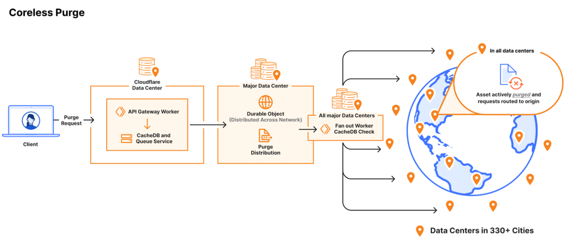
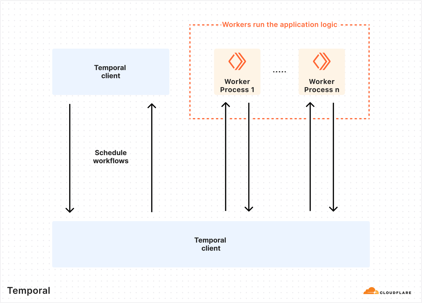
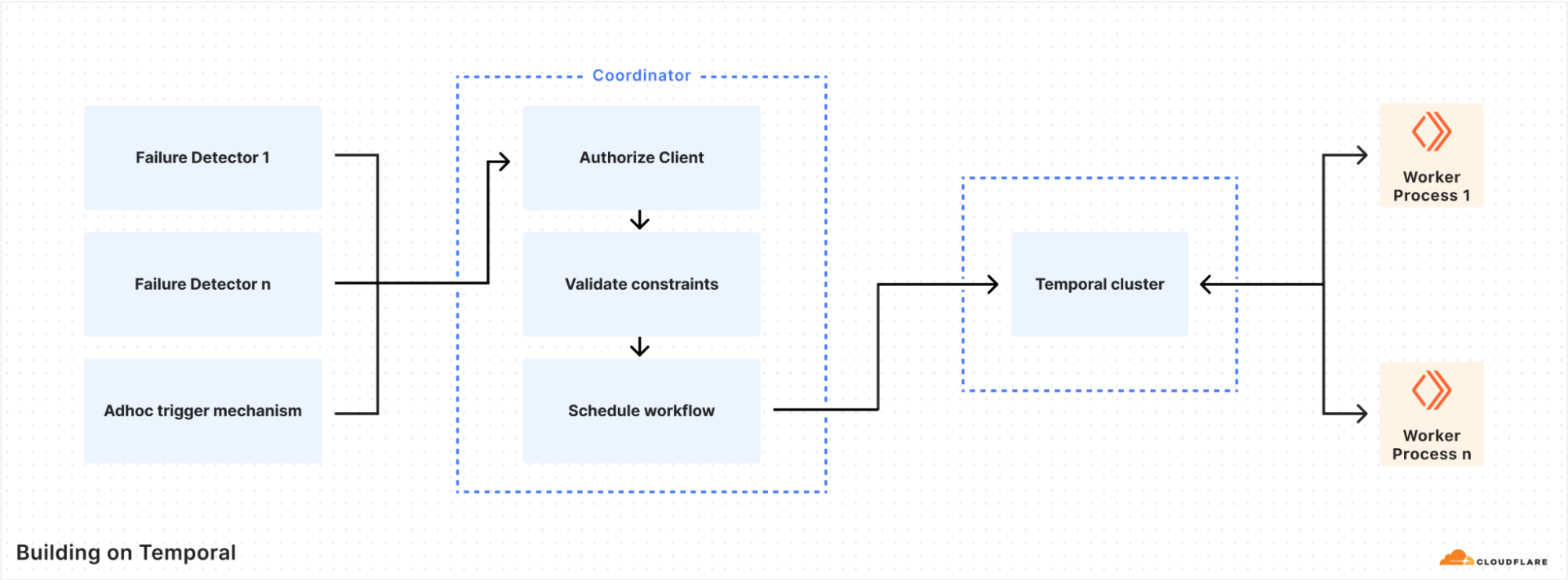
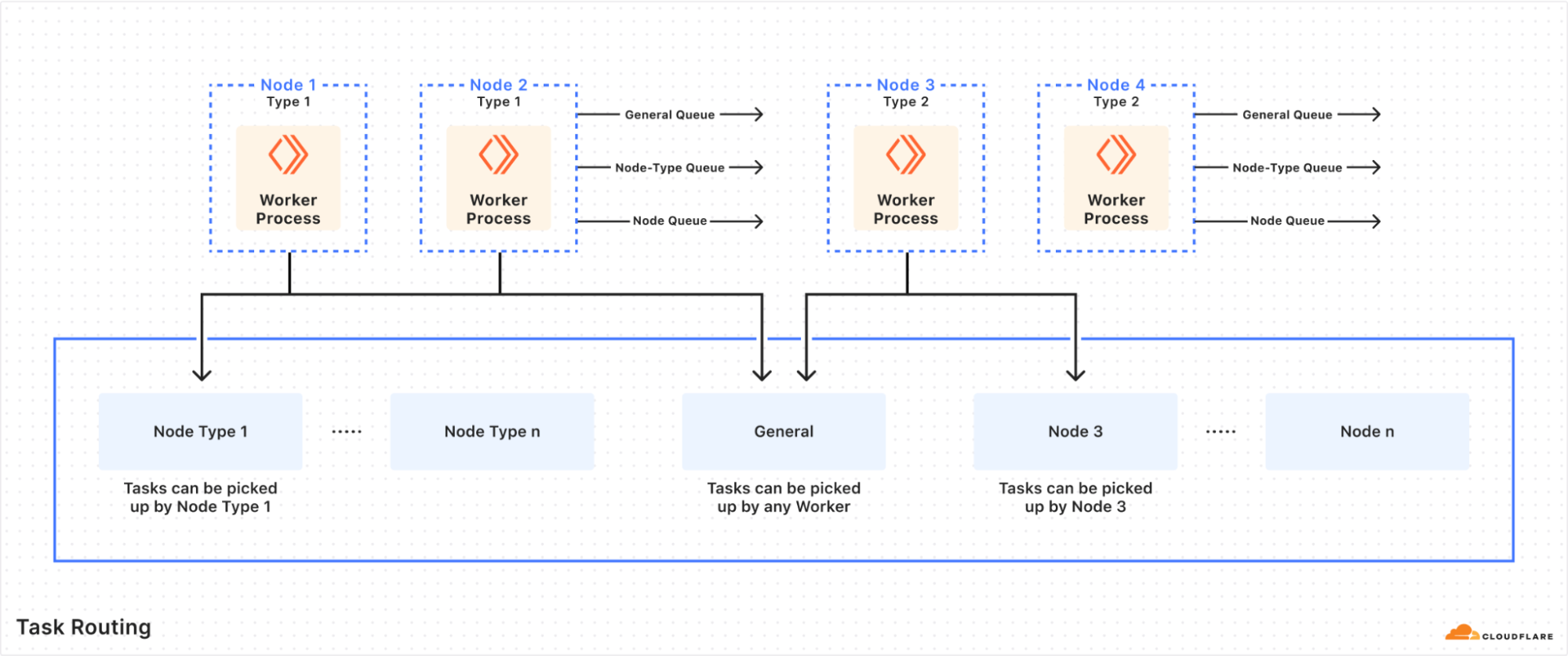
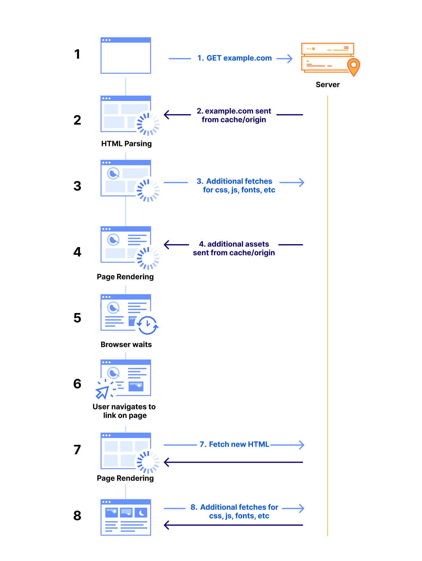
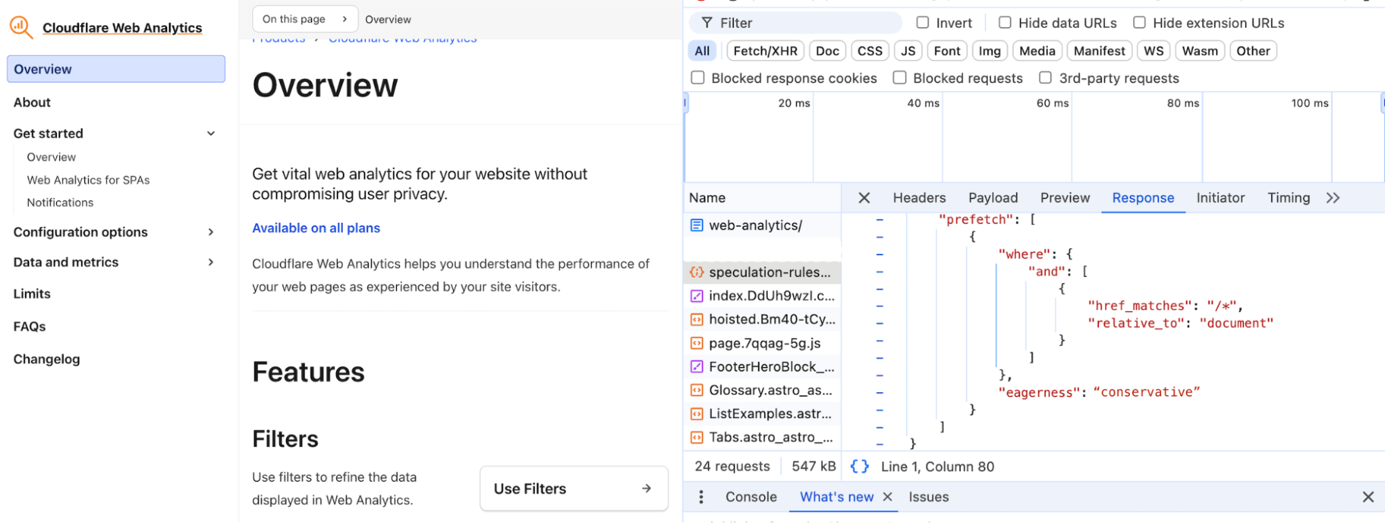
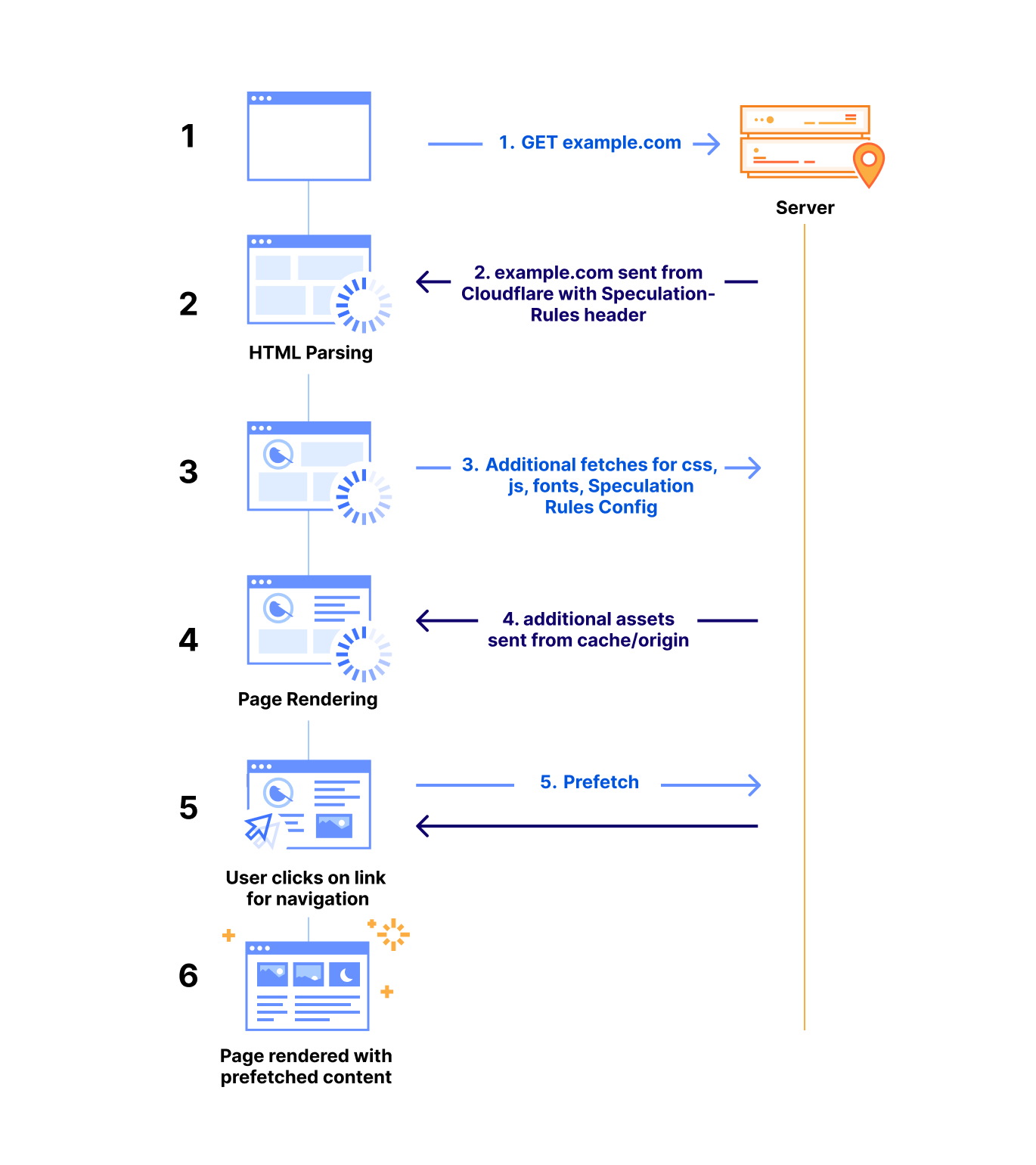
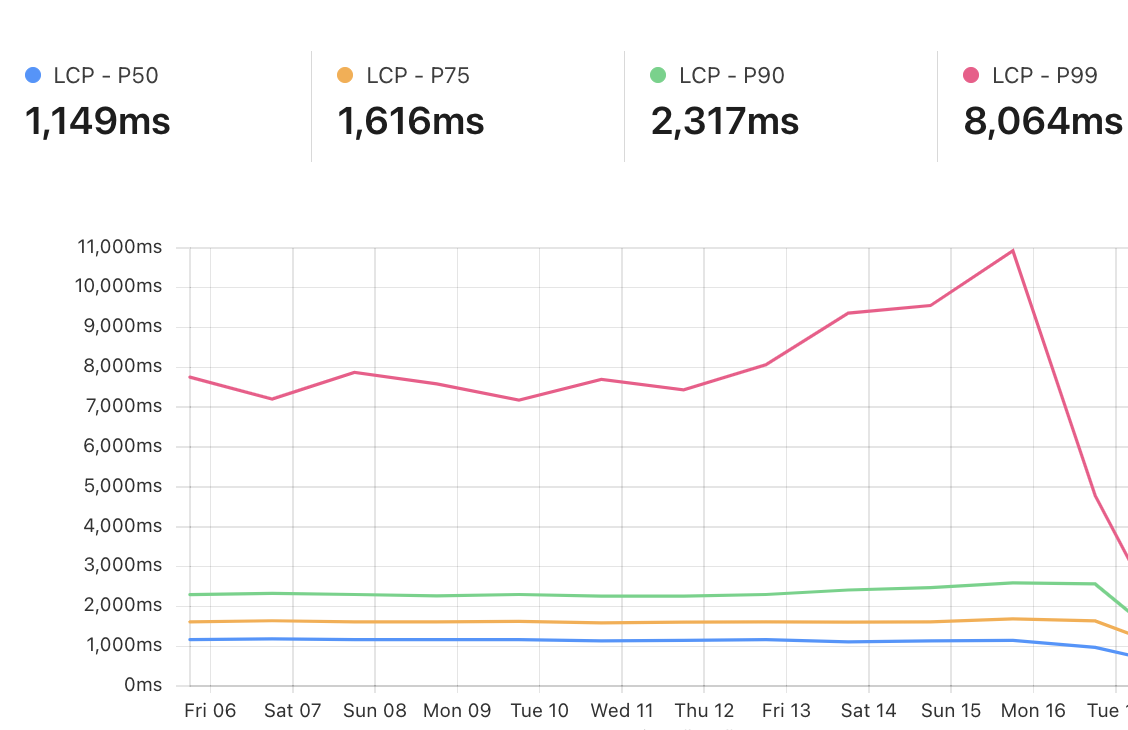
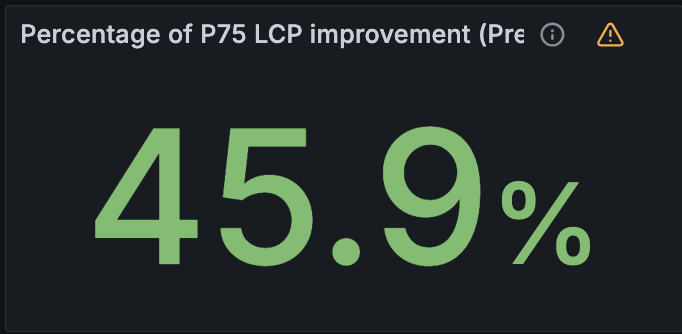
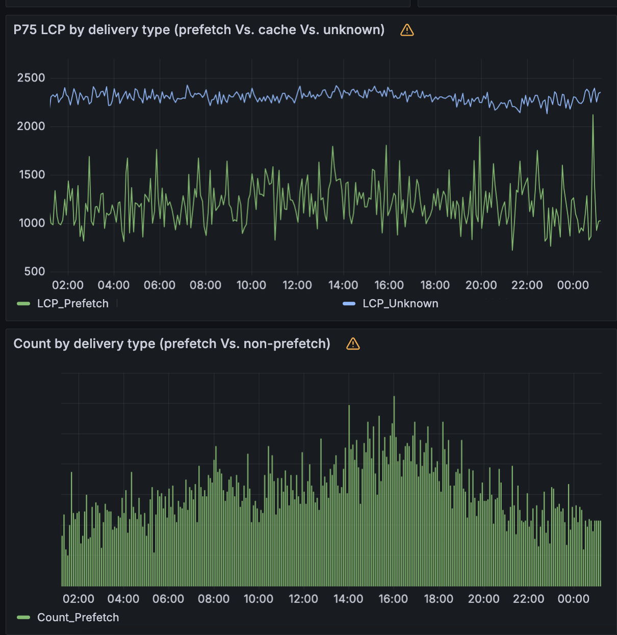

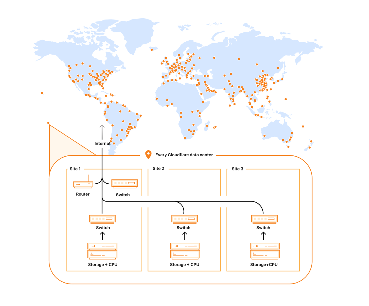
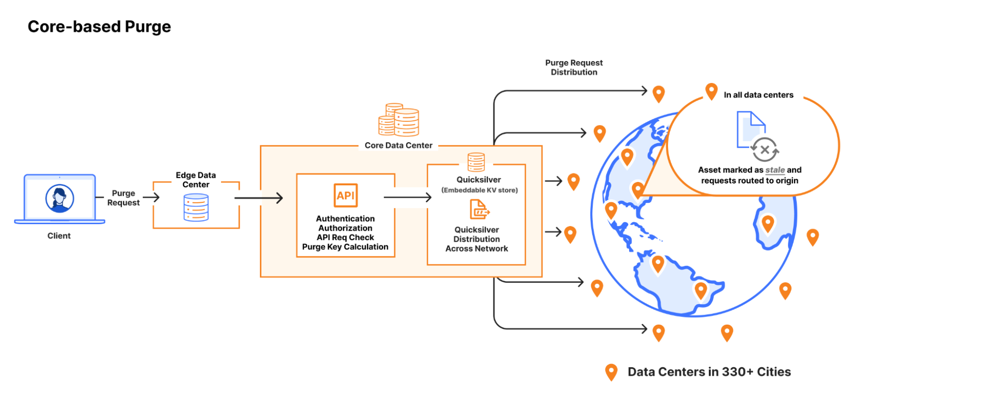
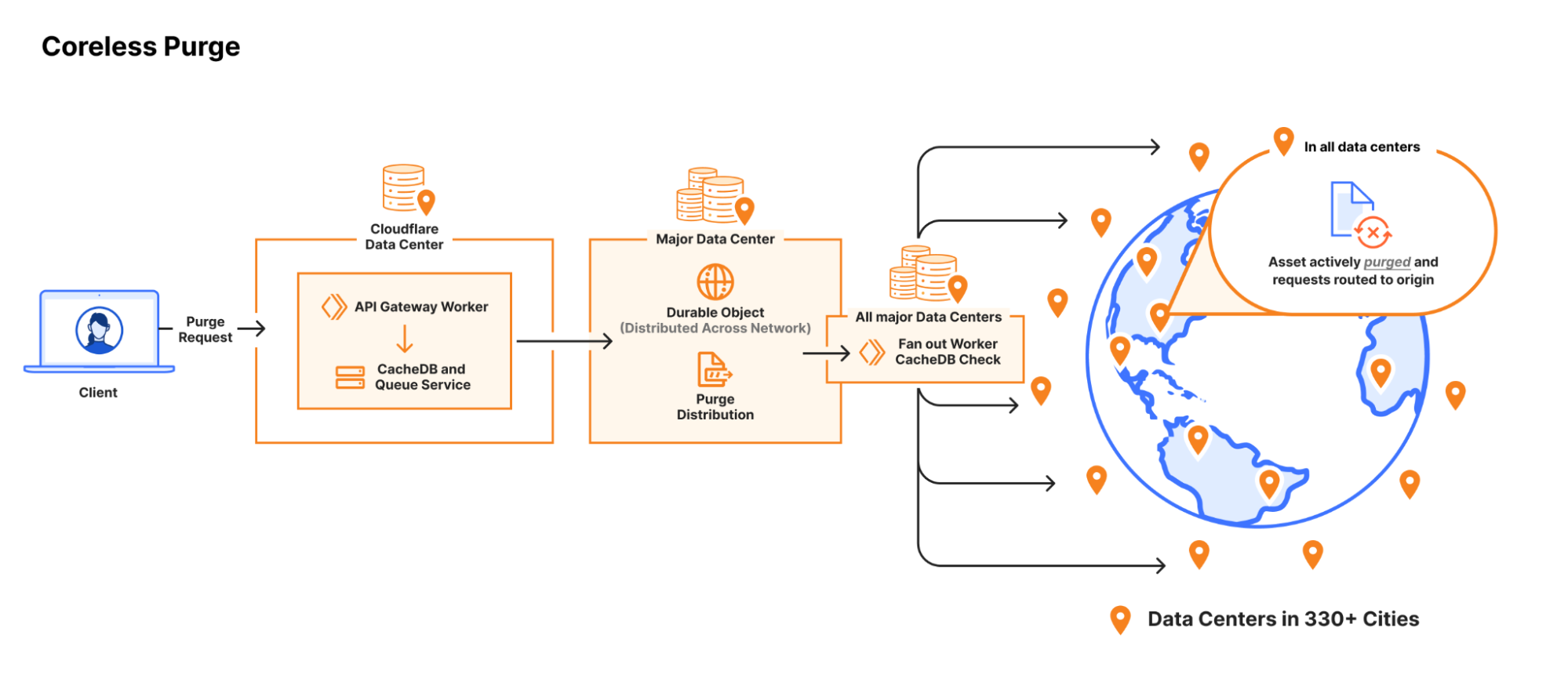
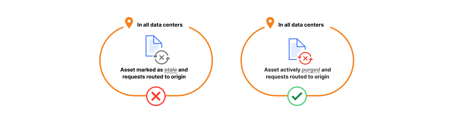
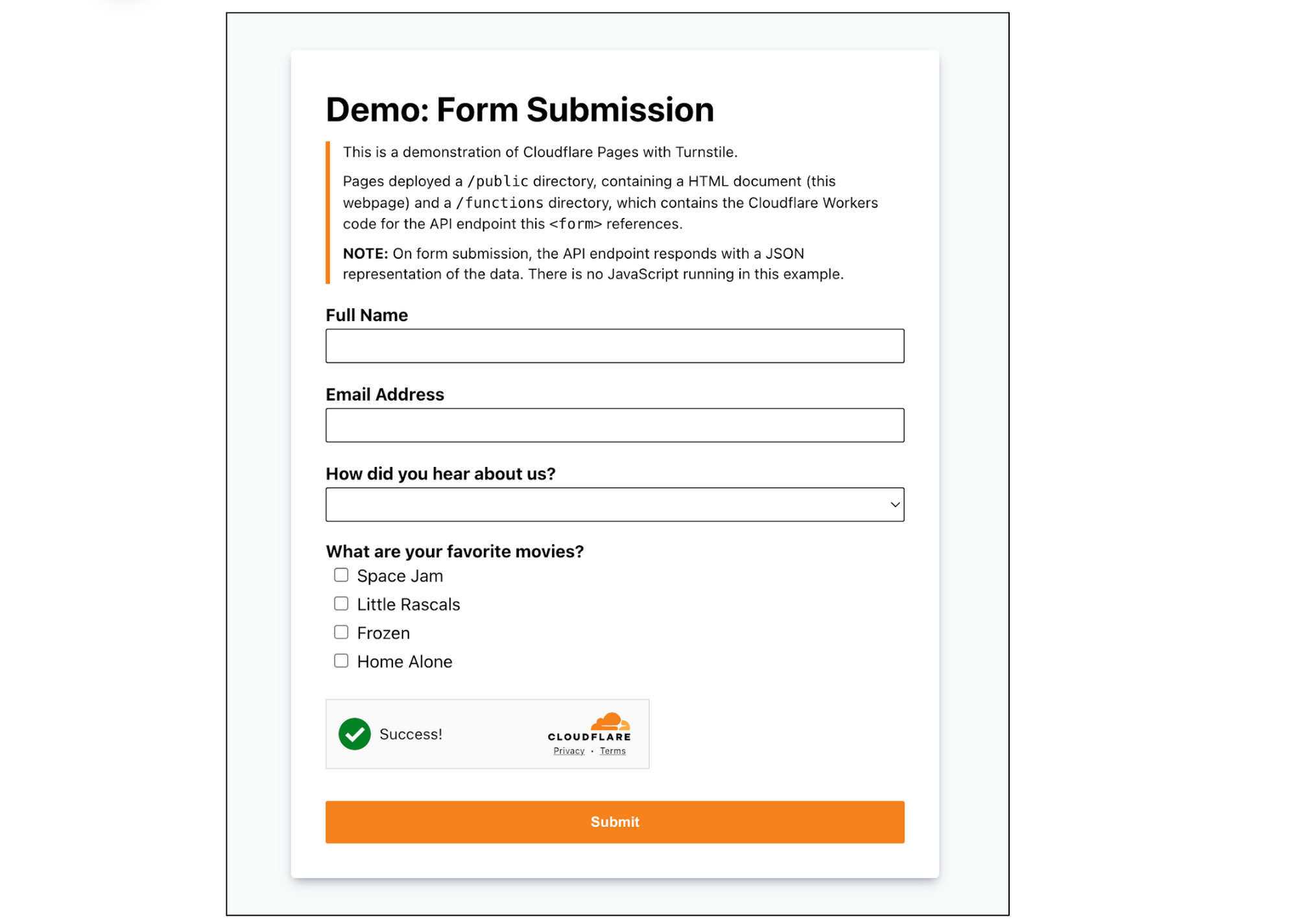
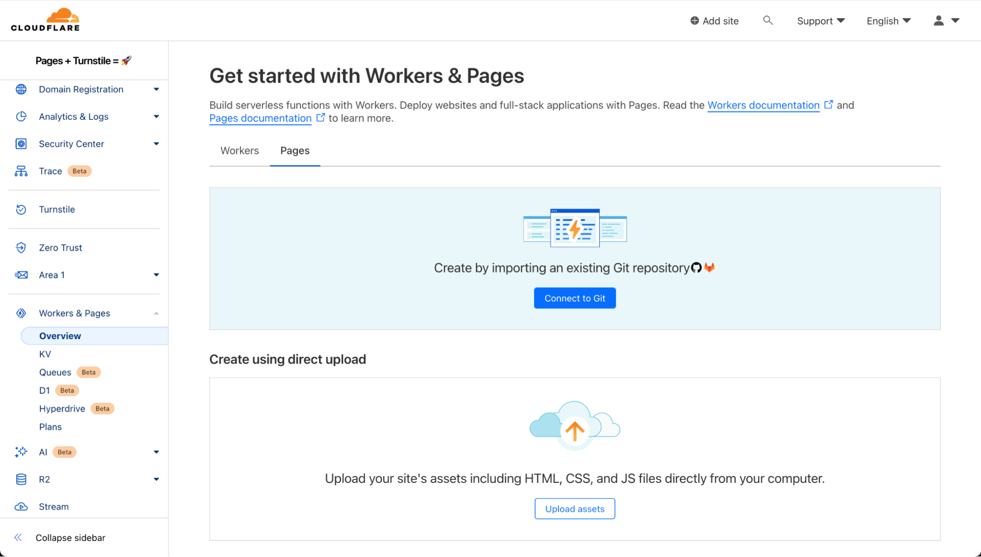
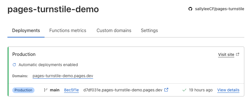


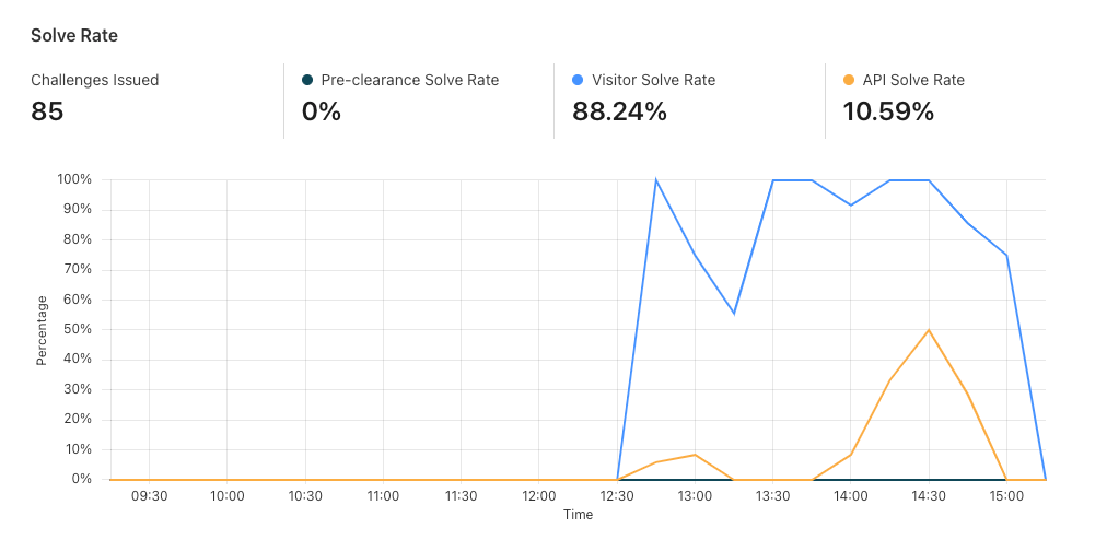
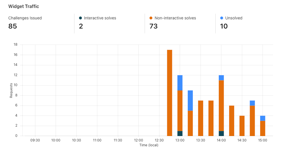


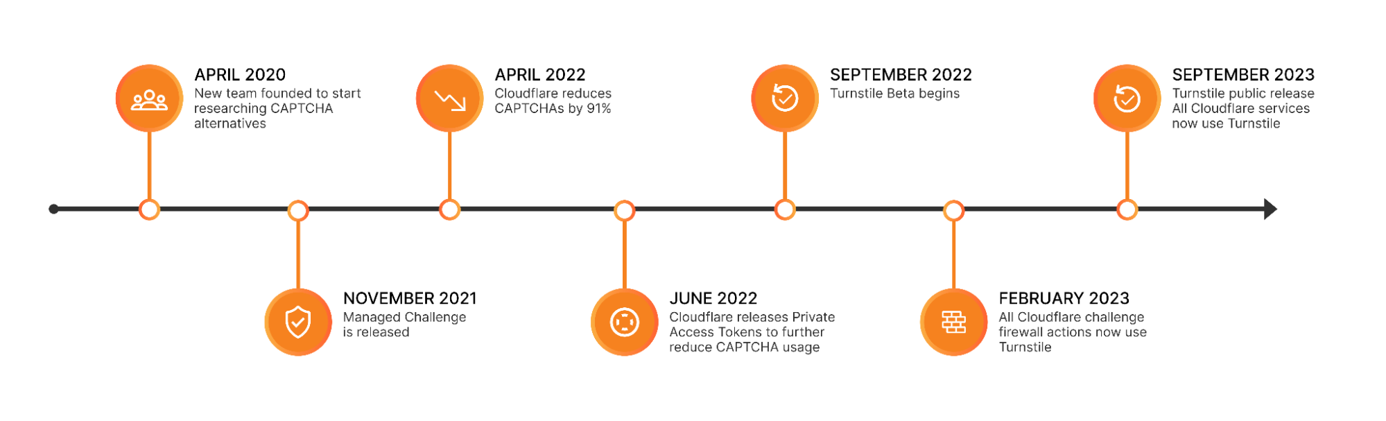


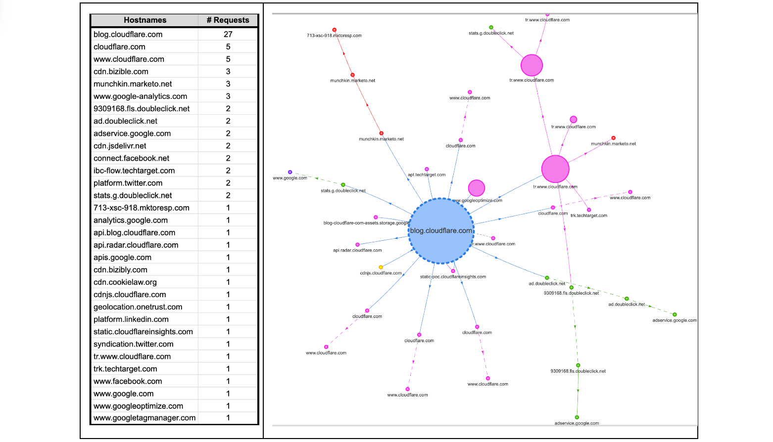
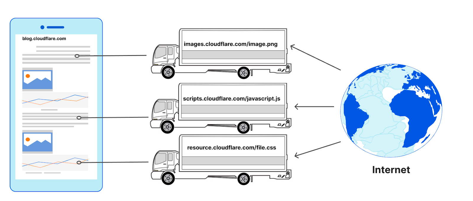
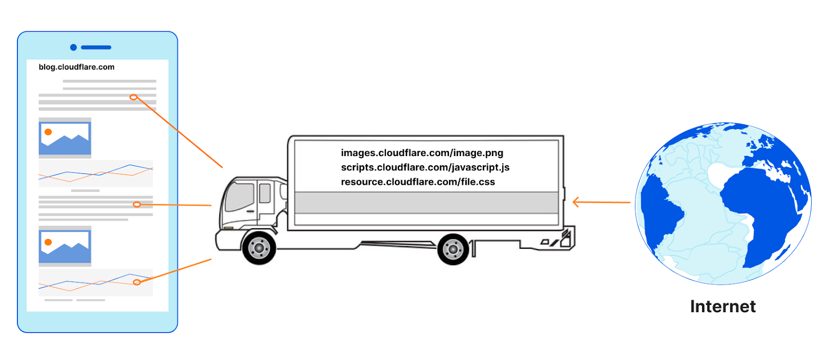
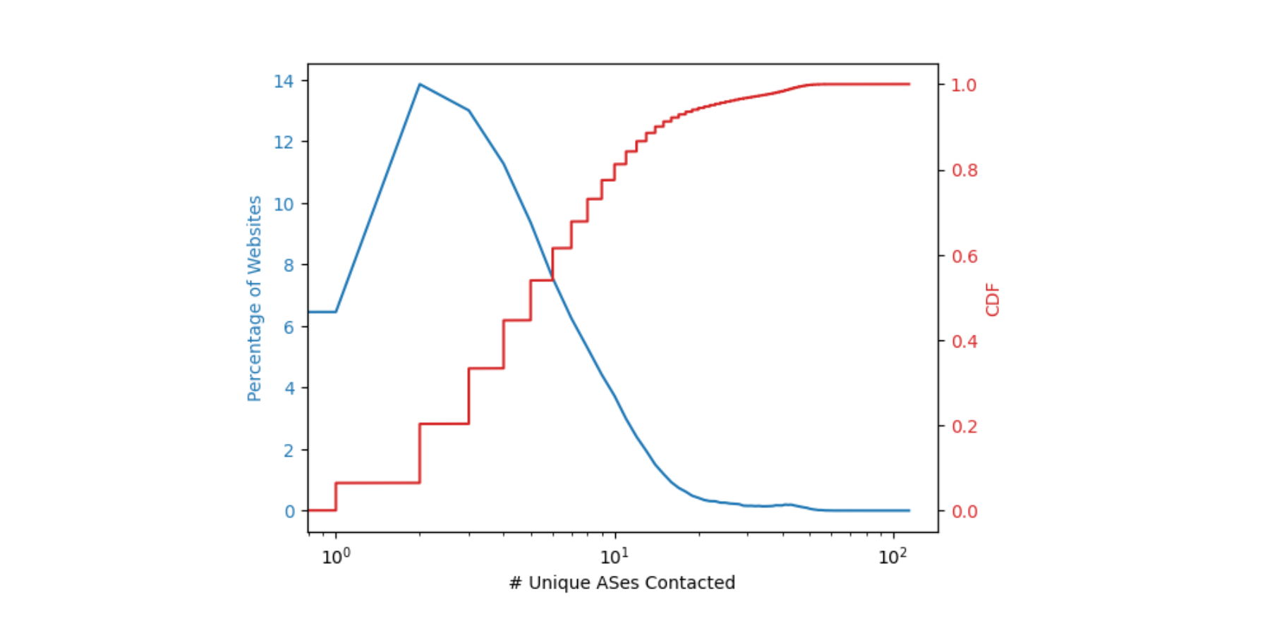
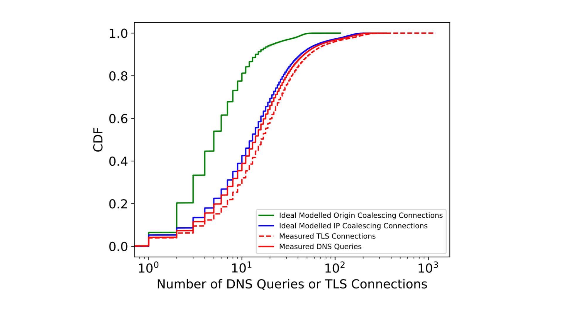
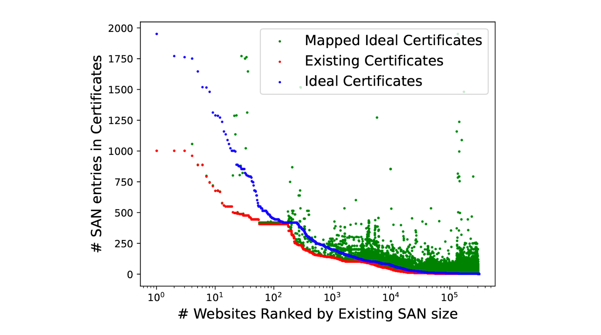
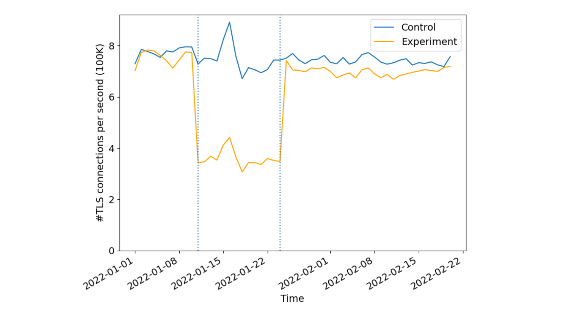

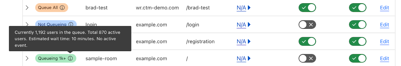
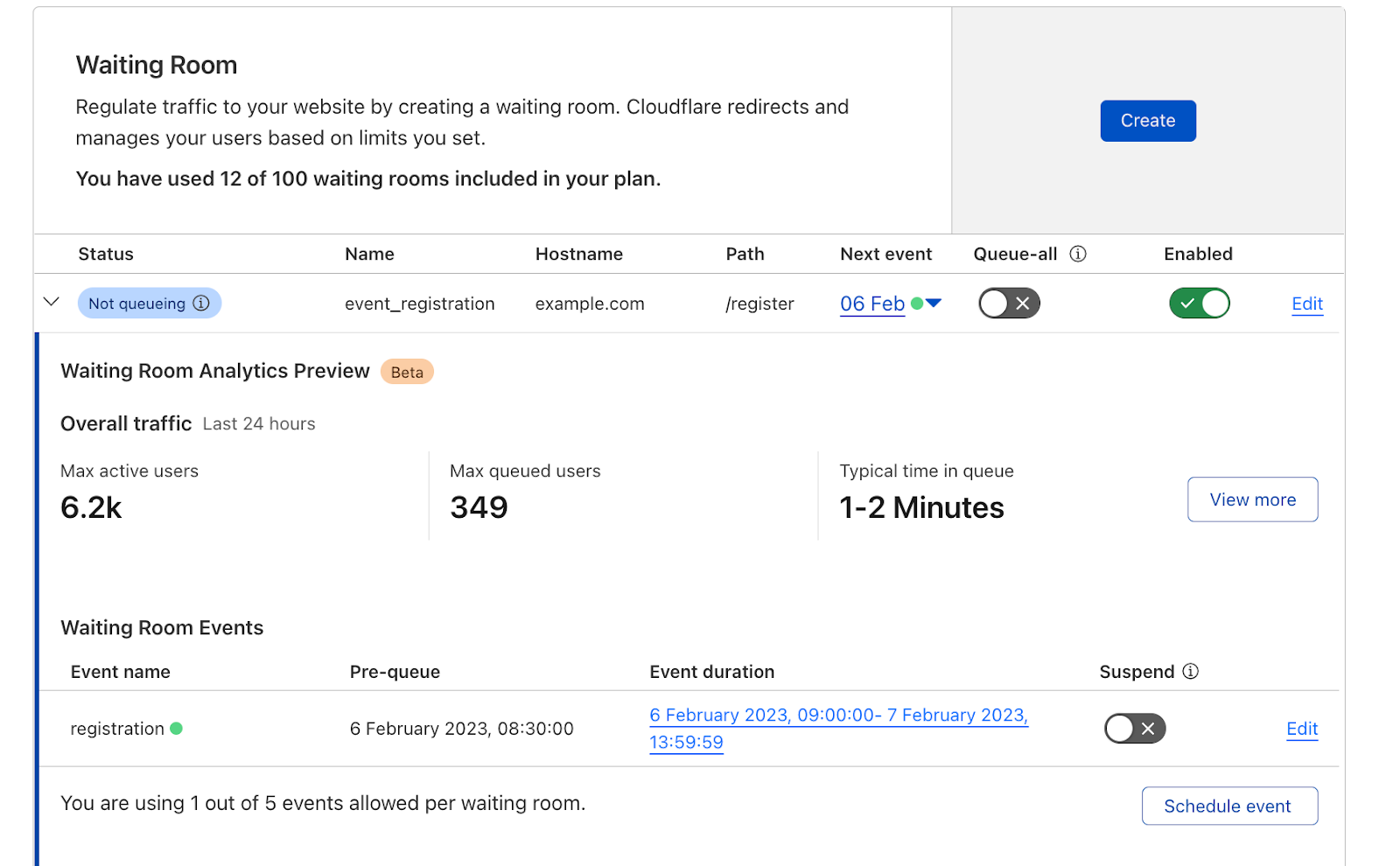

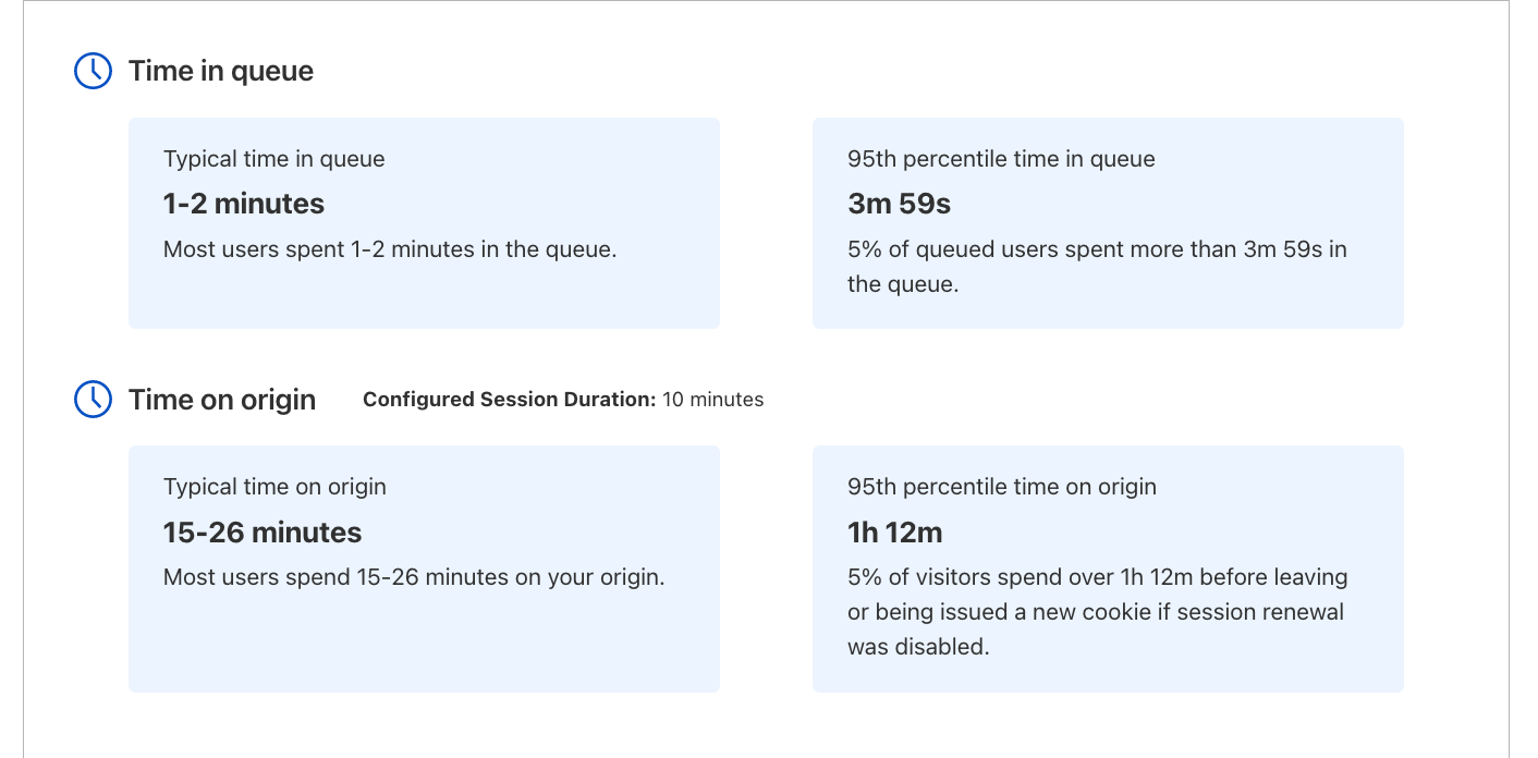
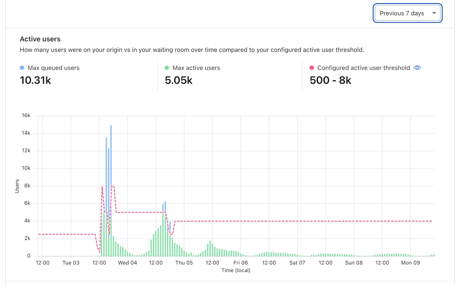
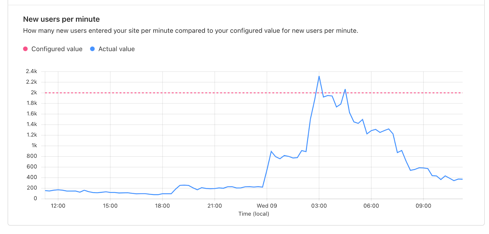
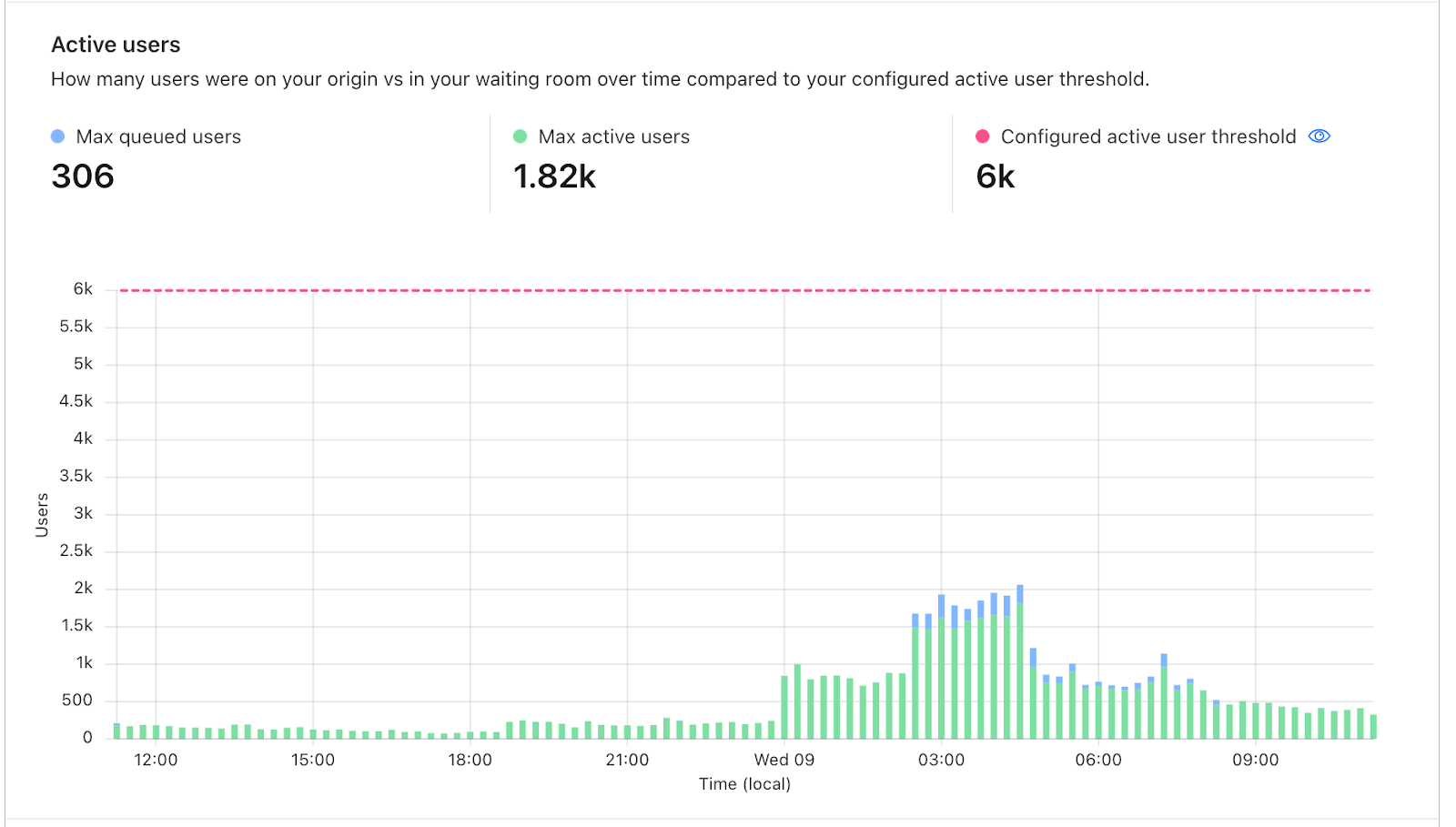
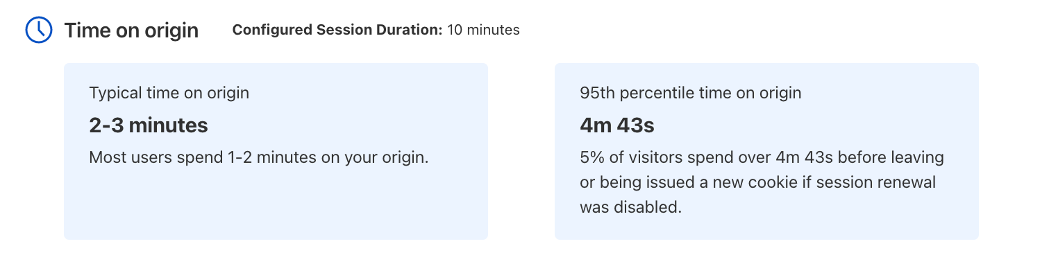
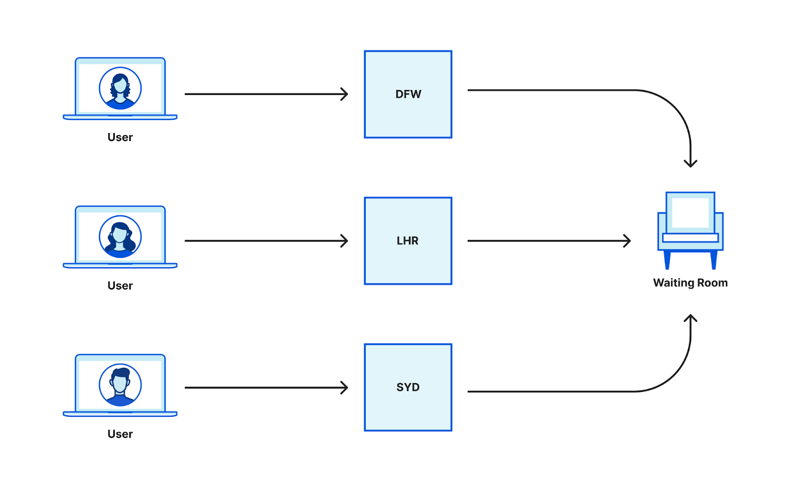
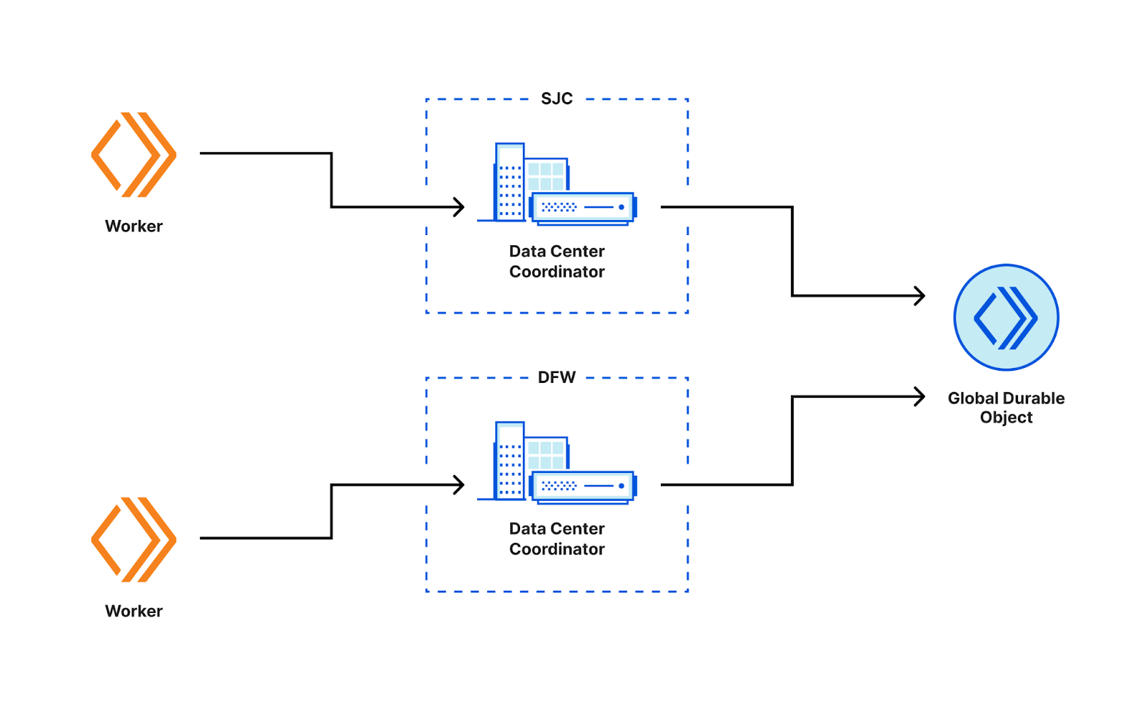


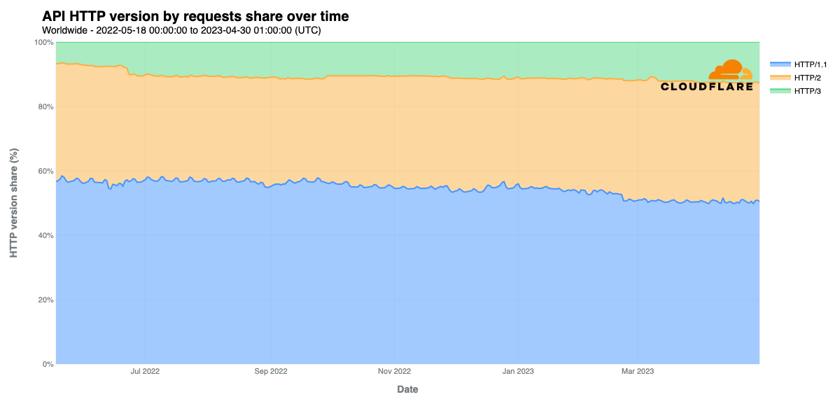


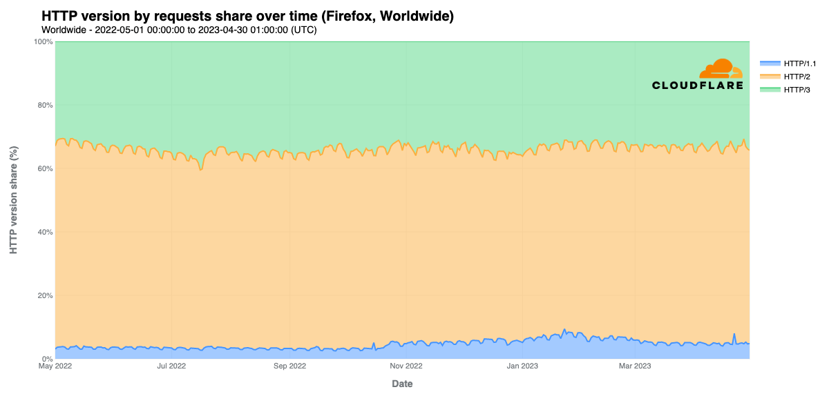


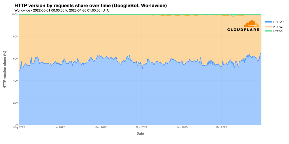


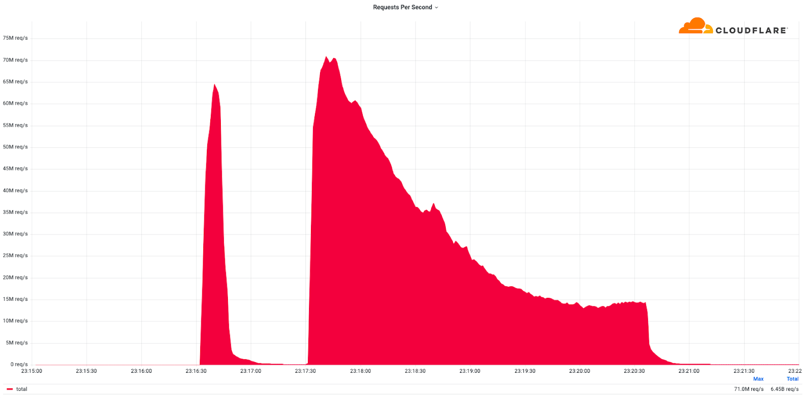
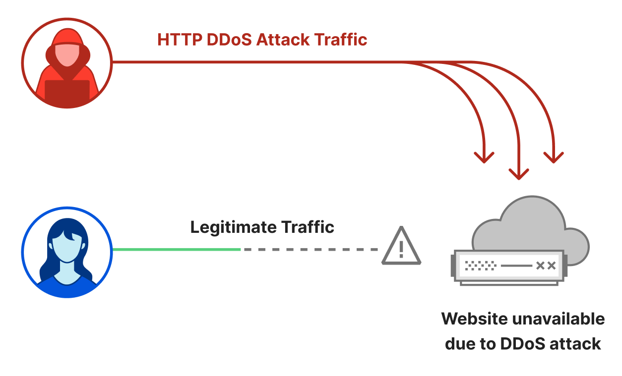
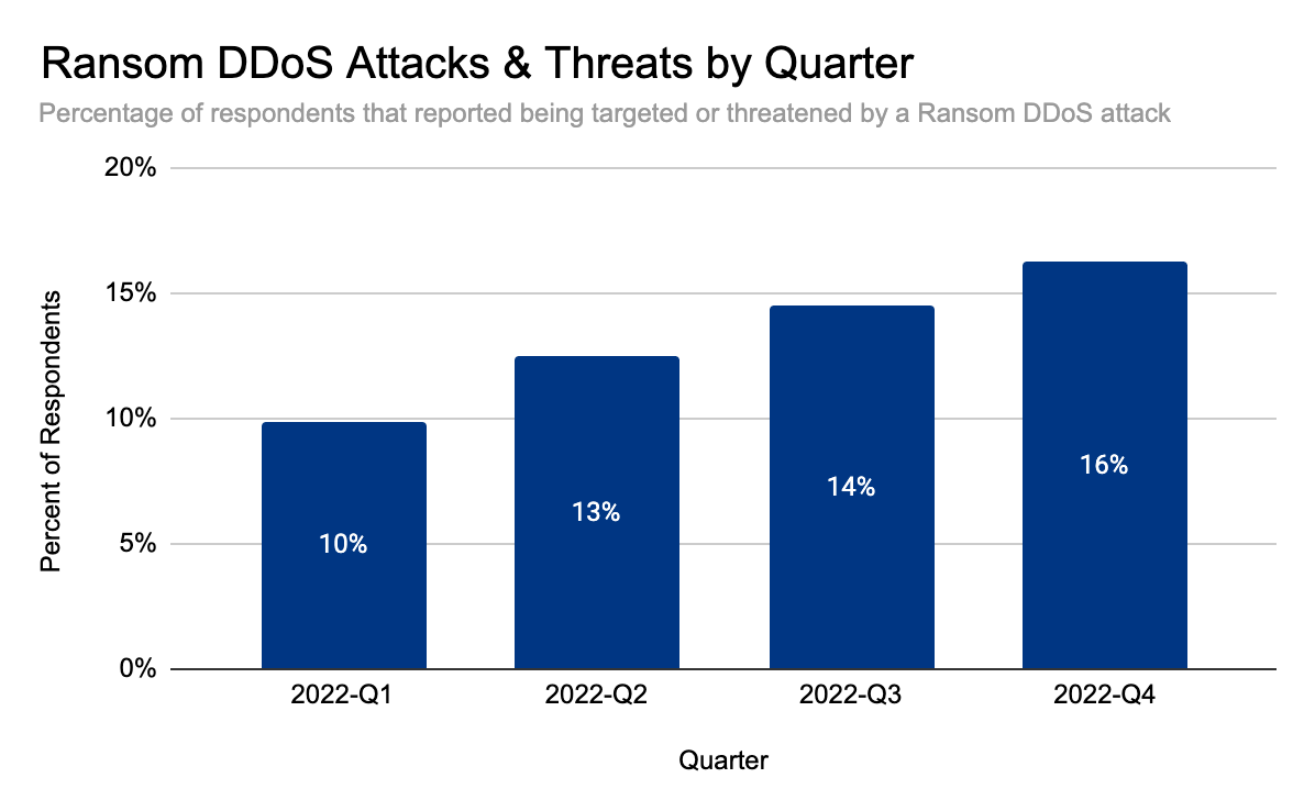


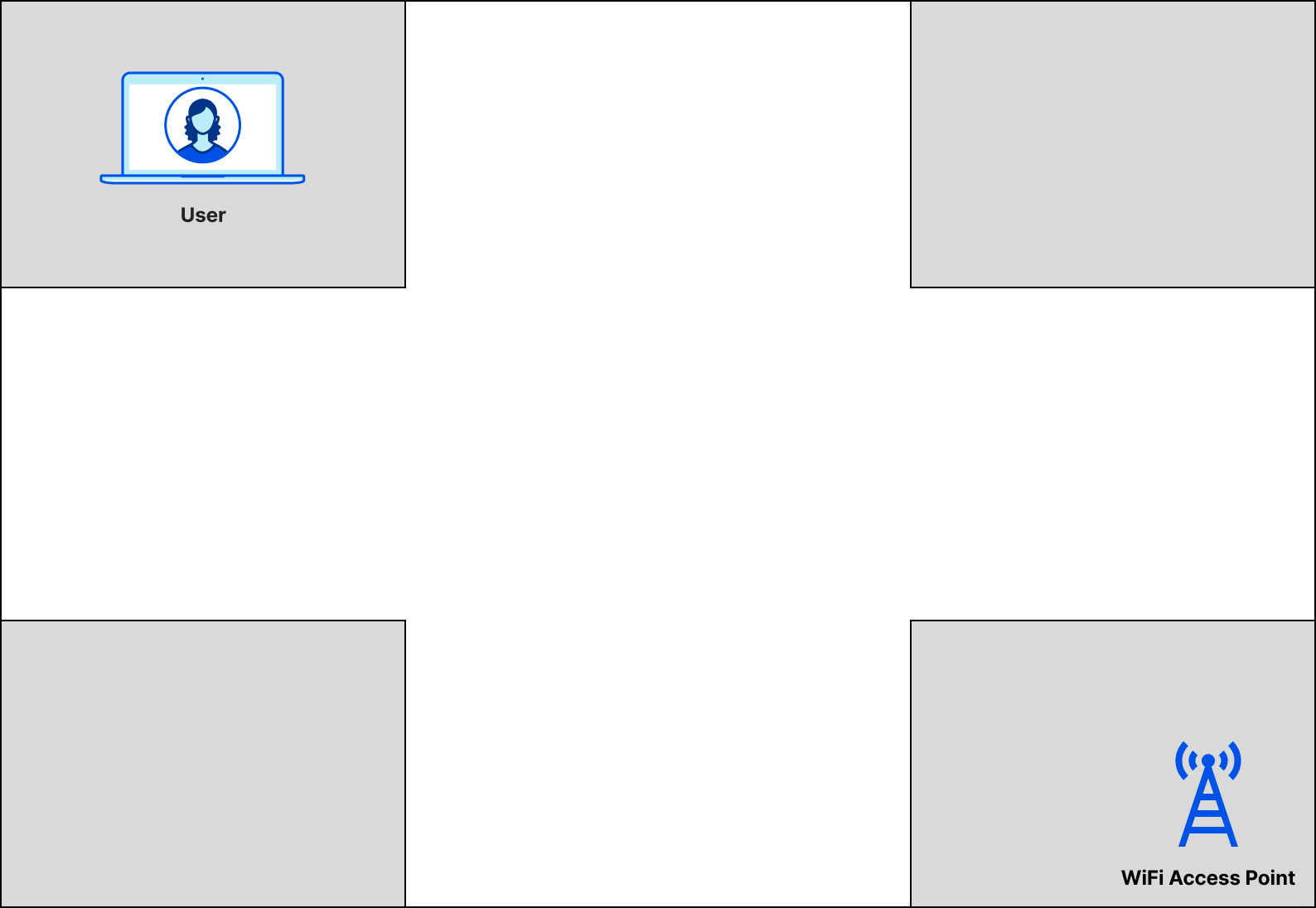
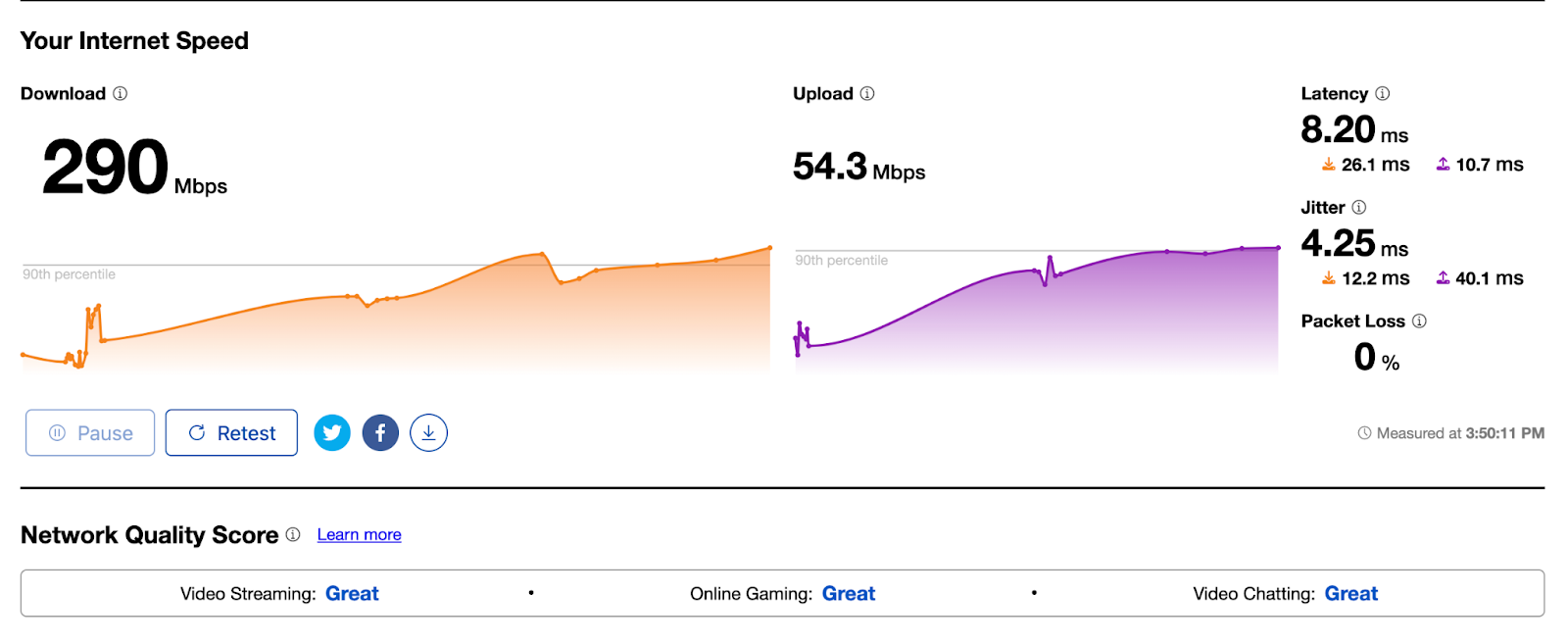
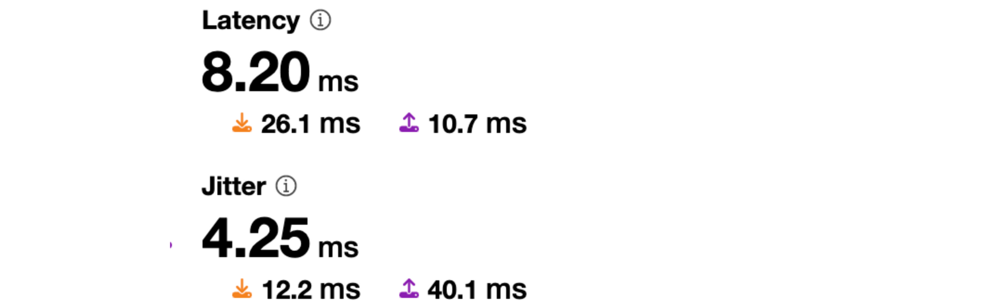
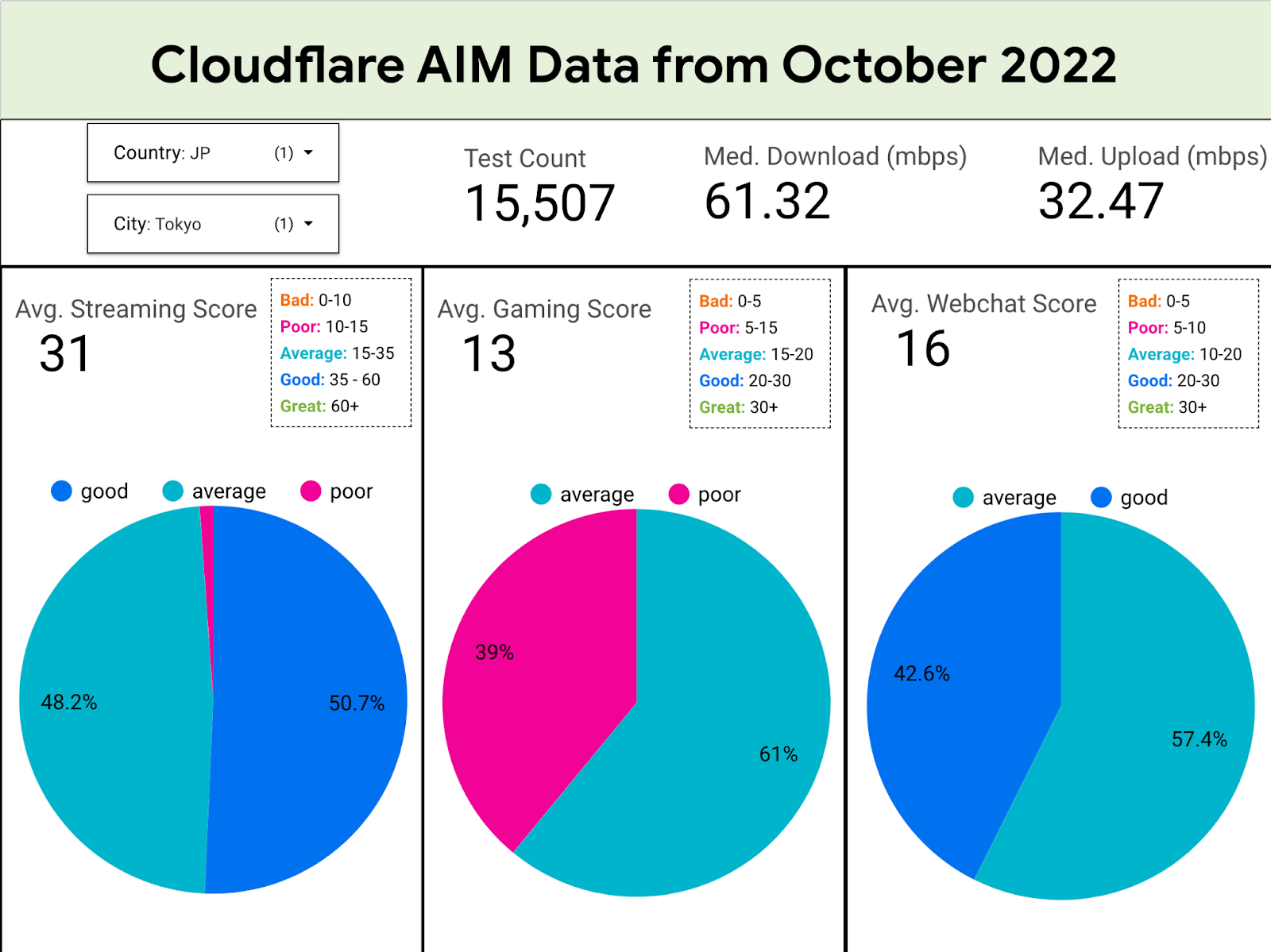


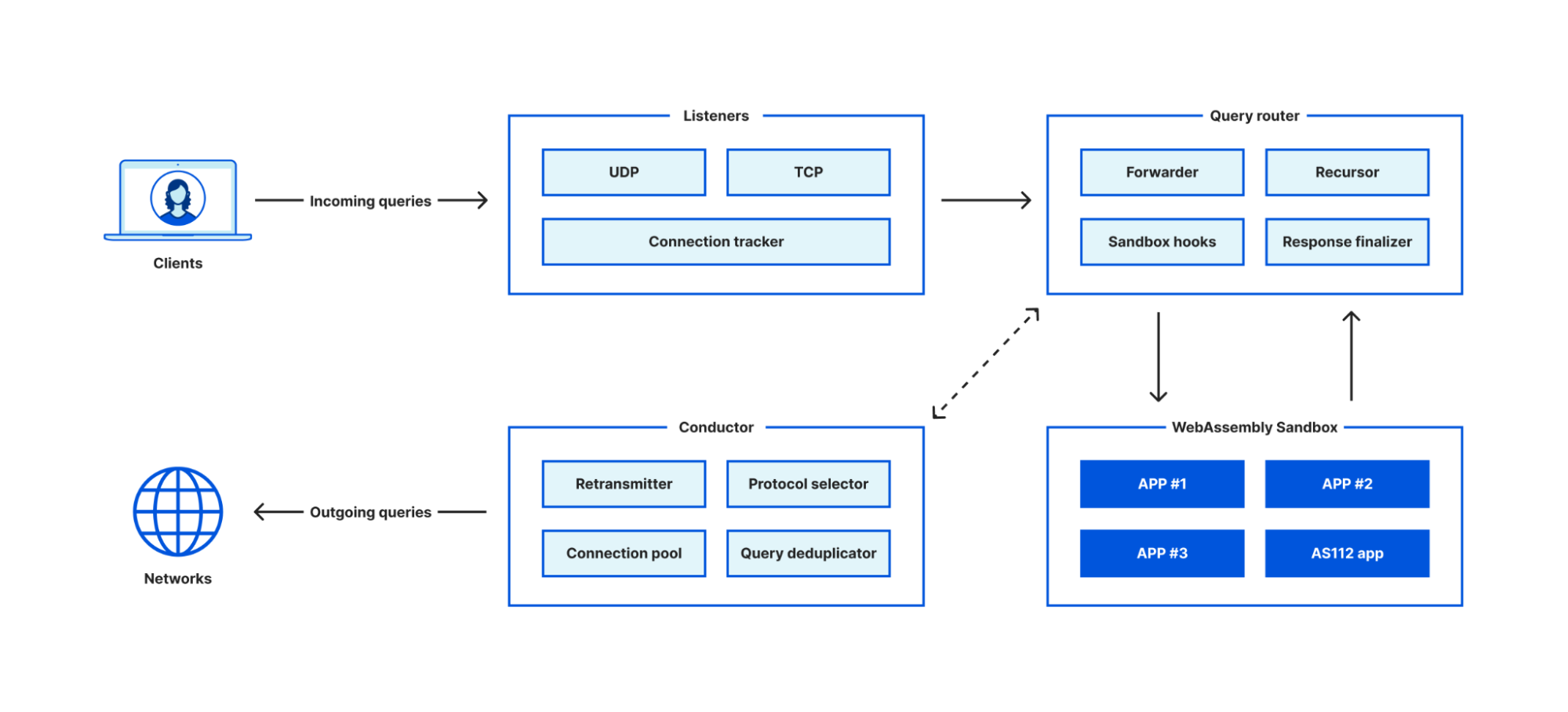
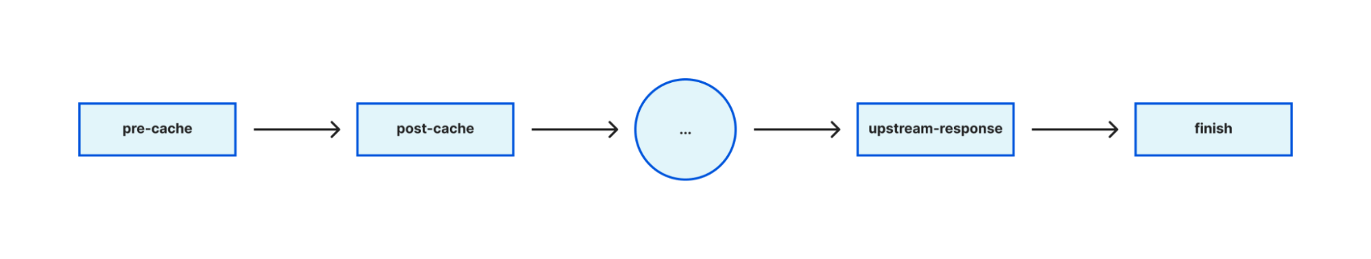


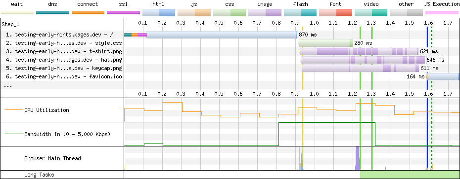
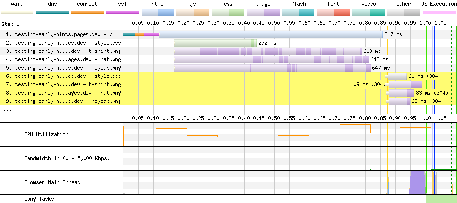


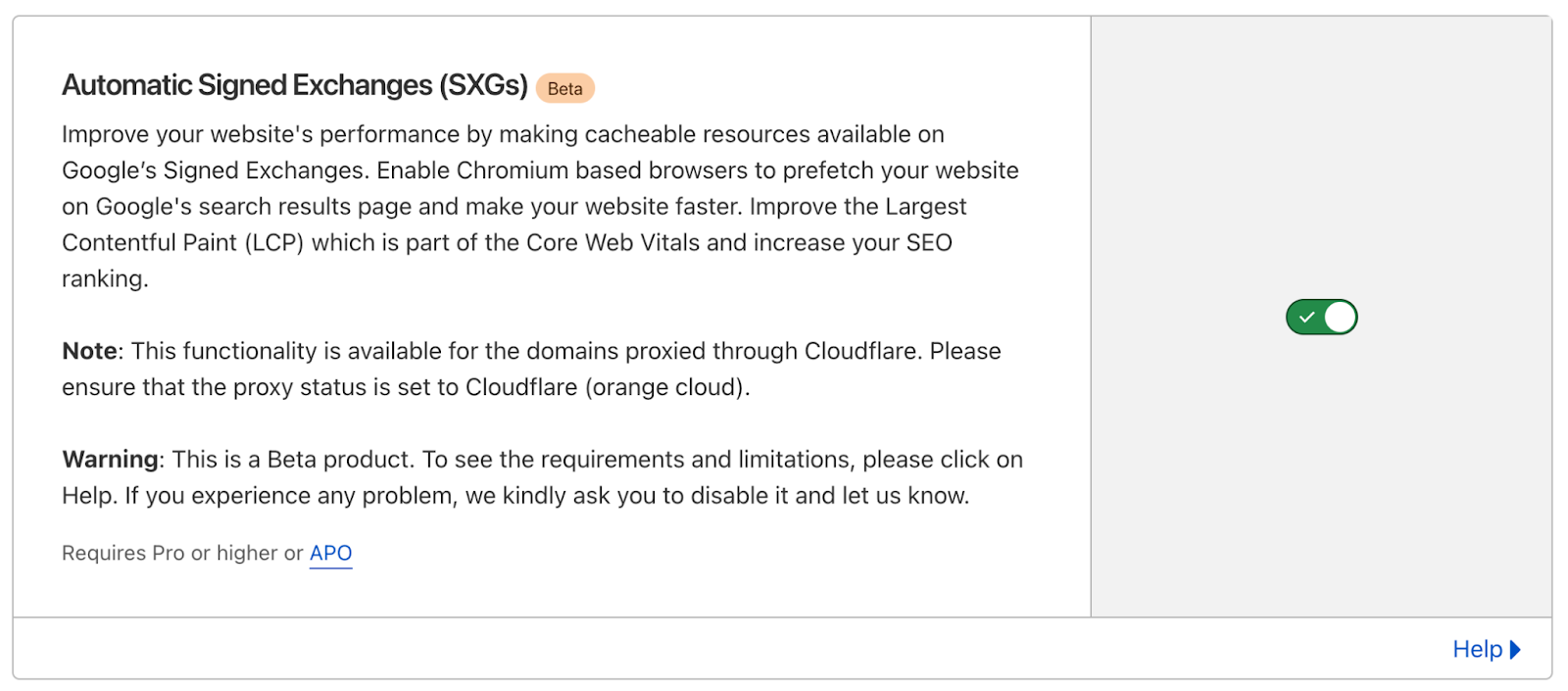
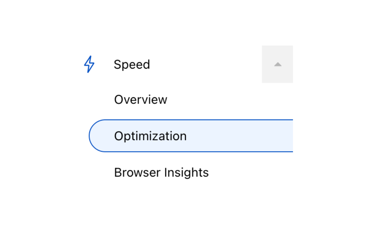


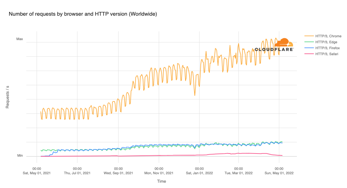
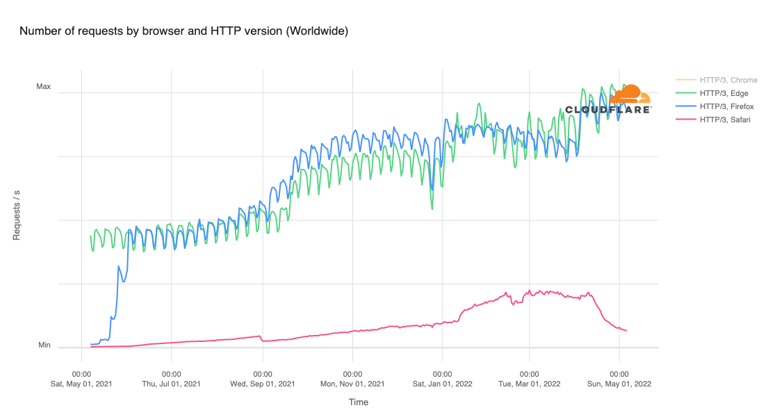
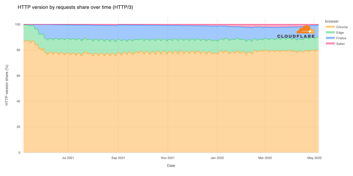
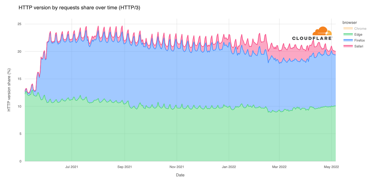
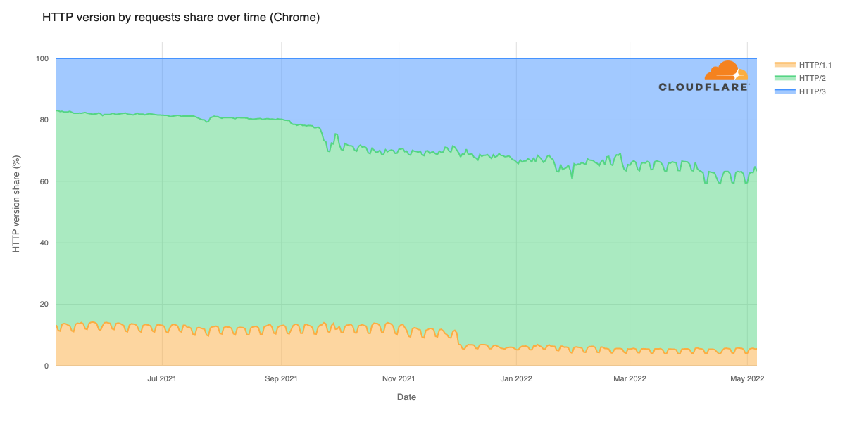
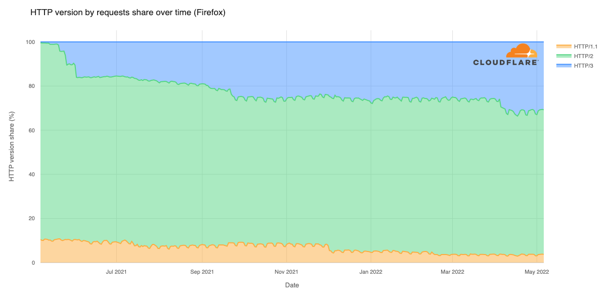
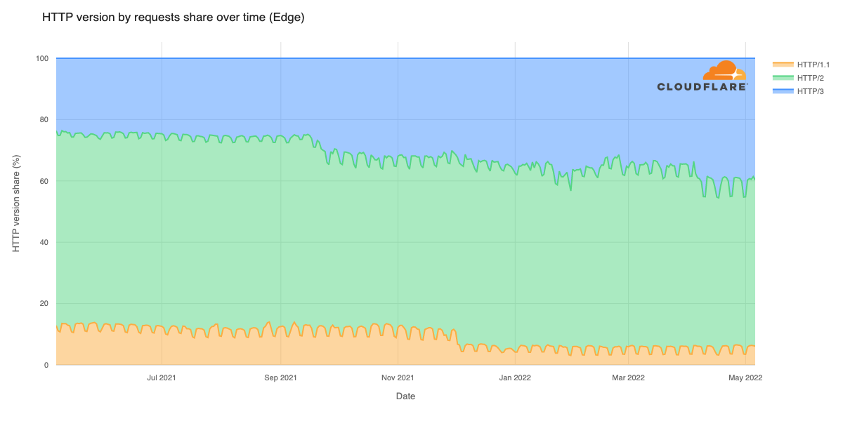
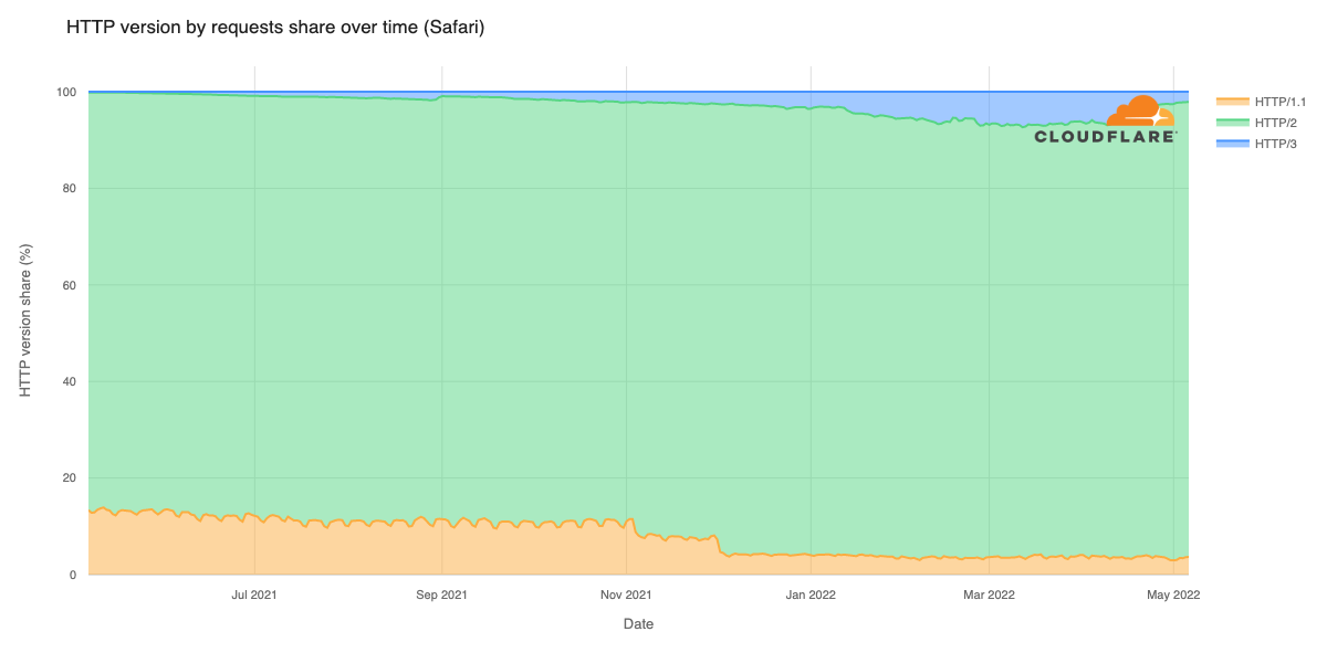
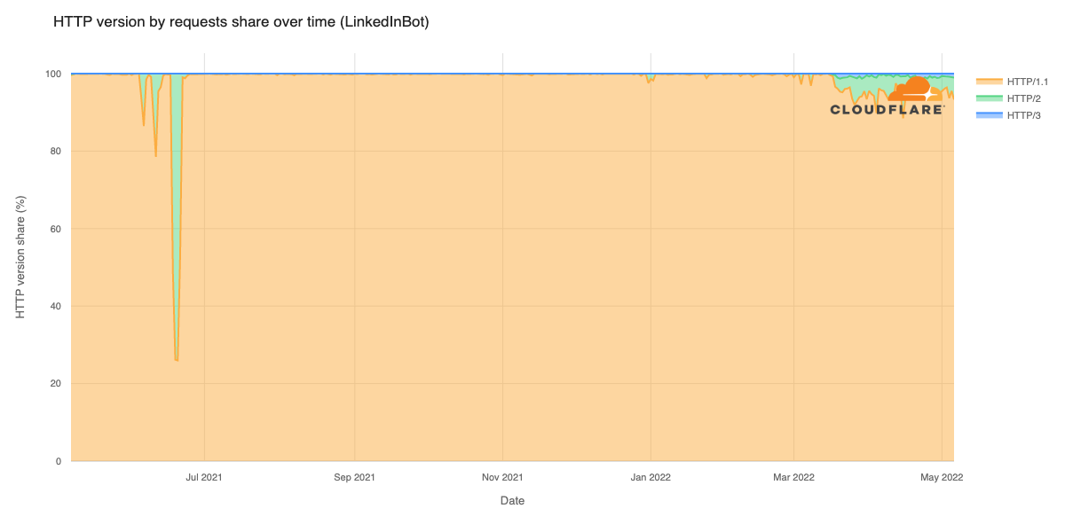


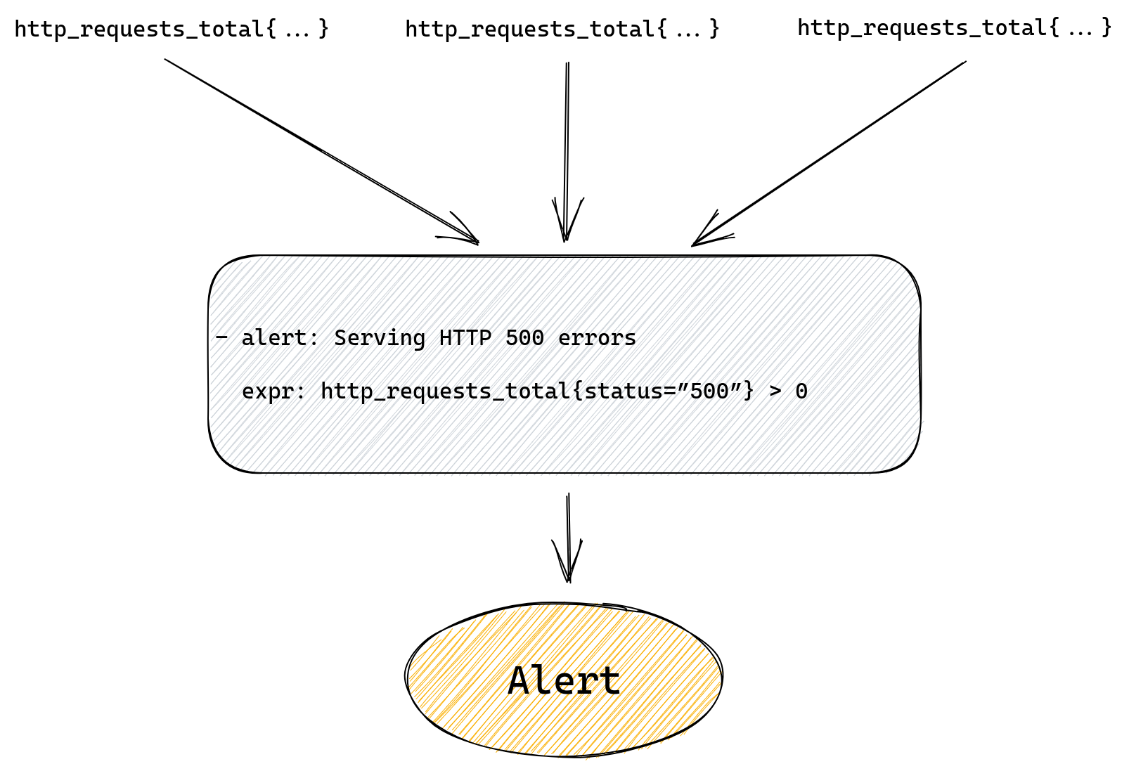
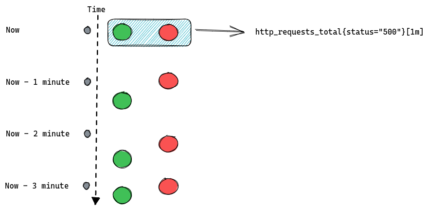
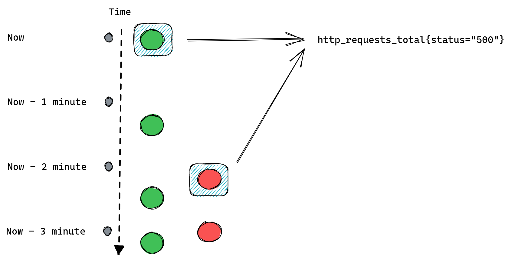
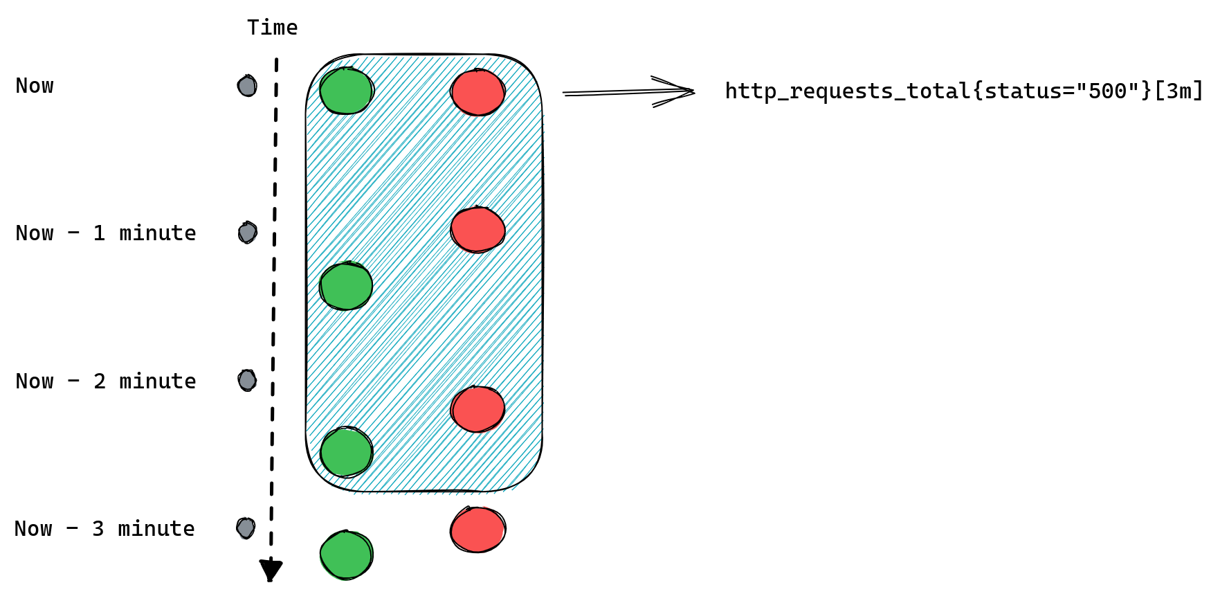
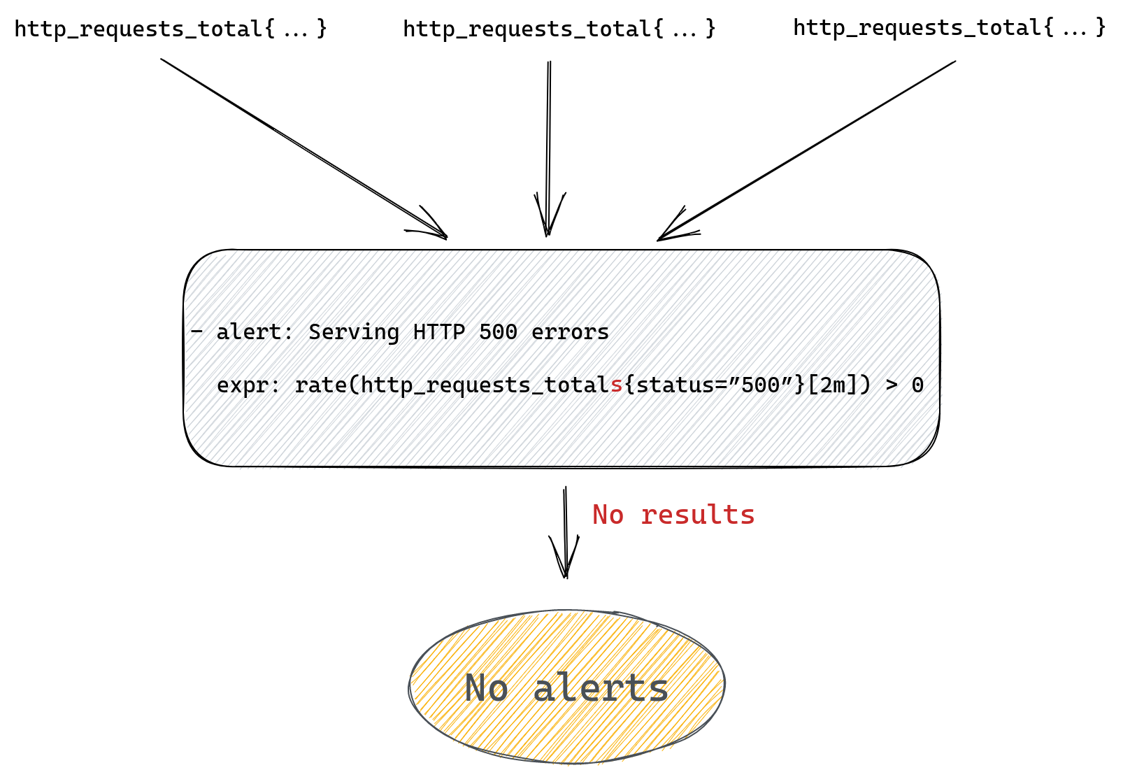
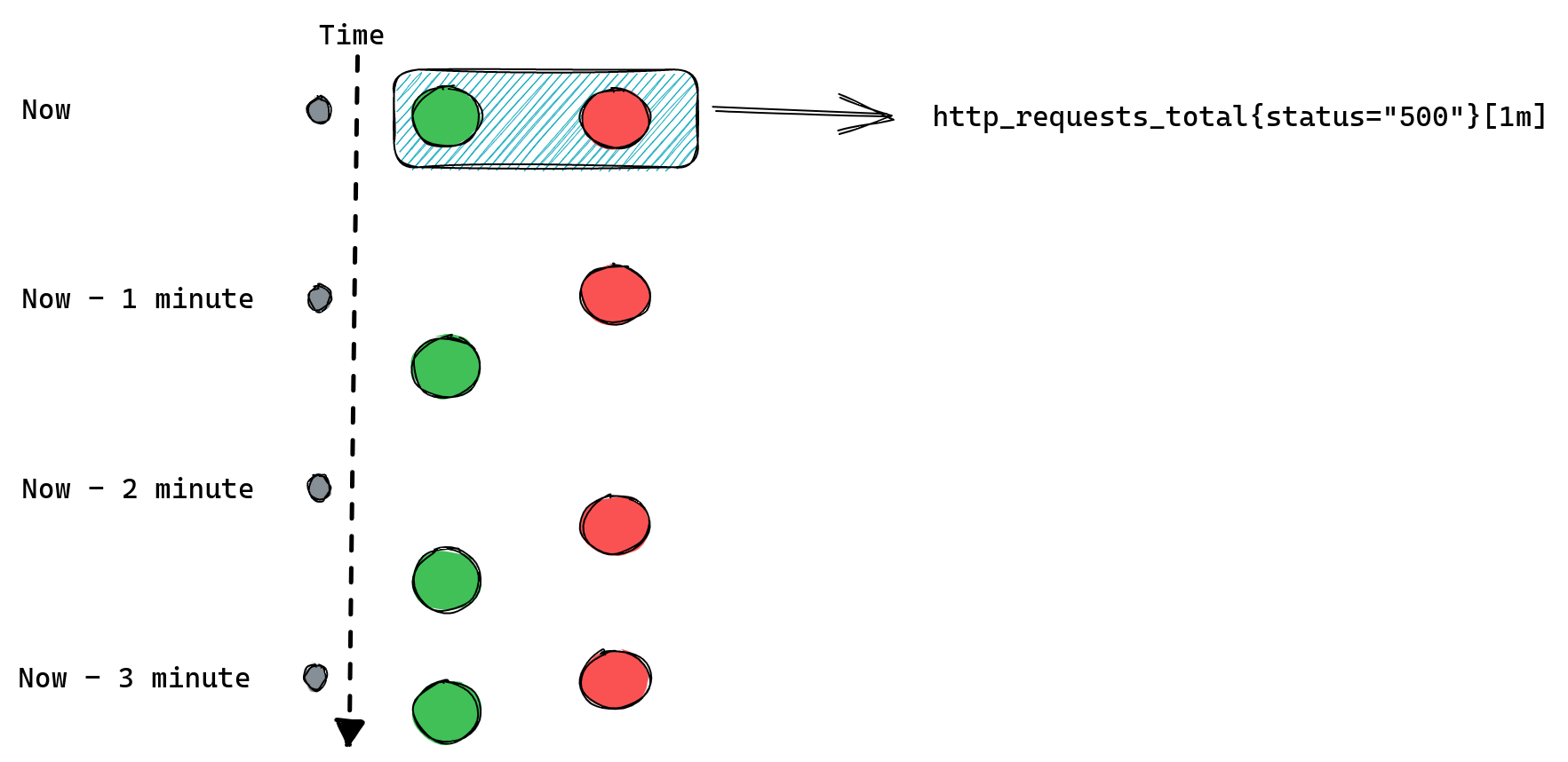
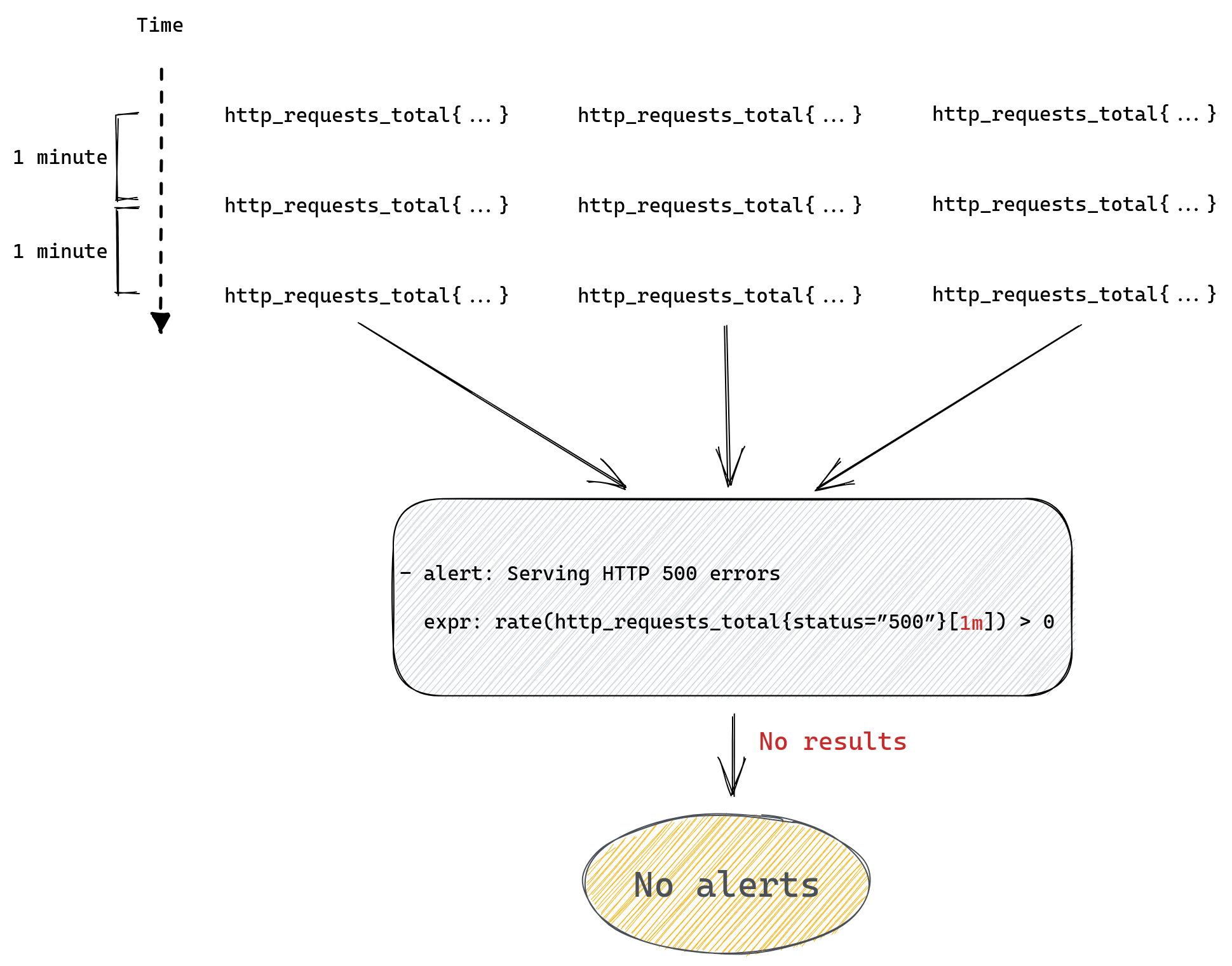
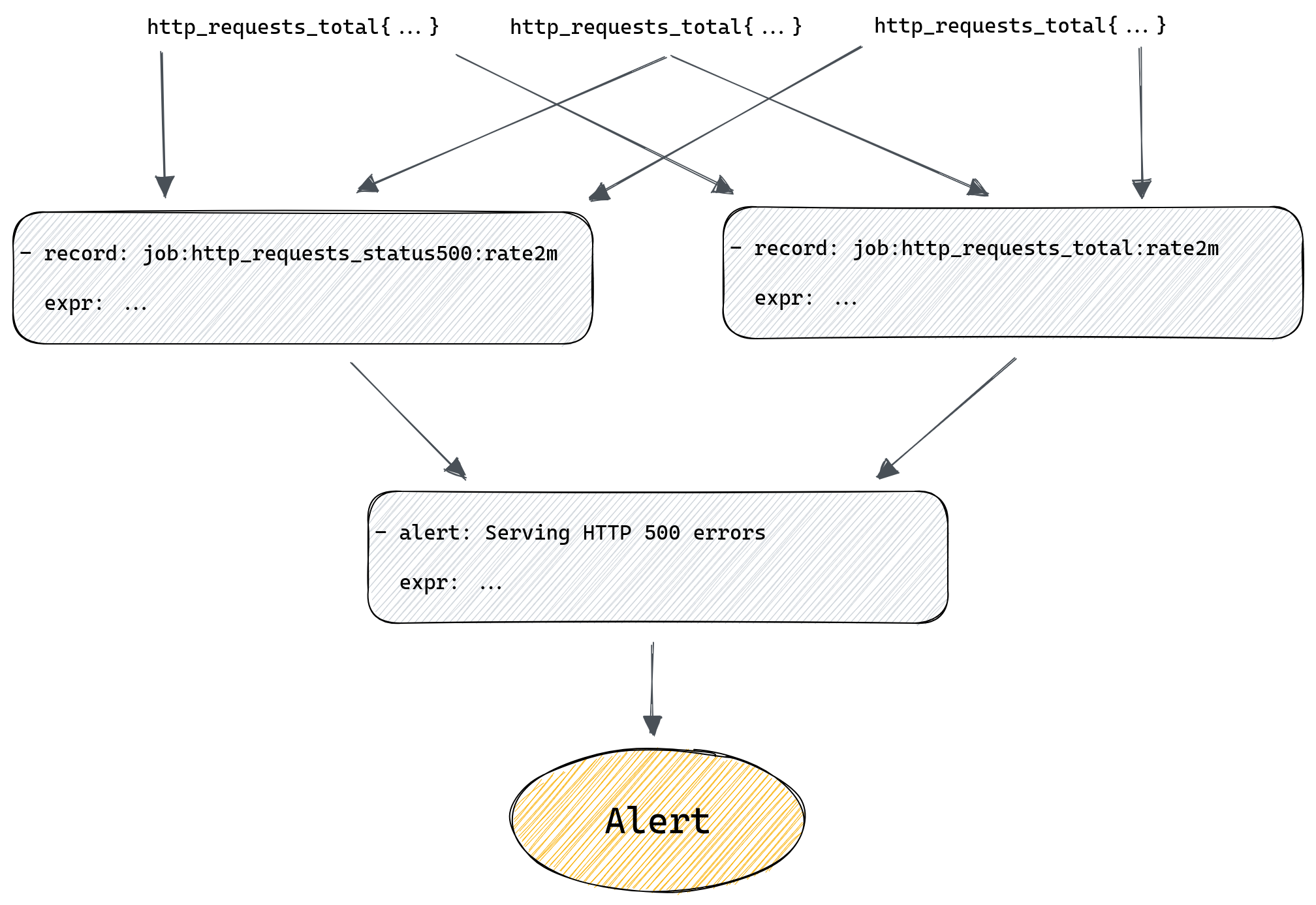
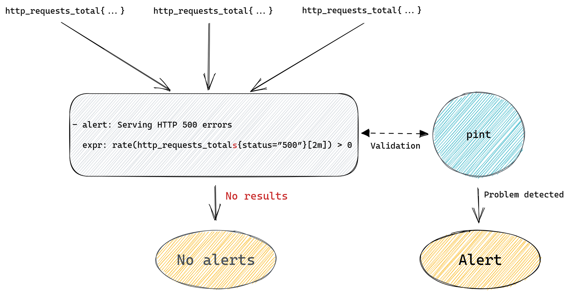


/ Pre-Performance Improvements")
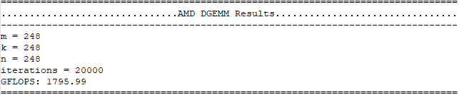
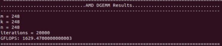


 / Post-Performance Improvements")