This post was co-written with Dr. Jan Melchior at BASF Digital Farming GmbH and xarvio Digital Farming Solutions.
BASF Digital Farming’s mission is to support farmers worldwide with cutting-edge digital agronomic decision advice by using its main crop optimization platform, xarvio FIELD MANAGER. This necessitates providing the most recent satellite imagery available as quickly as possible. This blog post describes the serverless architecture developed by BASF Digital Farming for efficiently downloading and supplying satellite imagery from various providers to support its xarvio platform.
Figure 1. Screenshot showing the xarvio Field Manager platform
Architecture
Figure 2 shows the serverless architecture implemented with AWS services for downloading and processing satellite imagery. The subscription management components handle subscription creation, updates, and deletions, while the actual data downloading and processing occurs in AWS Step Functions.
Figure 2. Serverless implementation of the new imagery service
Subscriptions are created using Amazon API Gateway for external API access, which provides request throttling and can be used to manage API request authorizations.
An AWS Lambda API function manages subscriptions. It implements common create, read, update, and delete operations with request validations and provides an endpoint for replaying failed requests. Subscriptions contain geometry, data provider, as well as start and end date and other parameters, which are stored in the subscription database (Step 7) before a message is sent out for processing. Notice that the entire architecture is serverless and thus allows for theoretically unbounded scaling. In case of a bug, this can lead to severe cost impacts, so we implemented a safety buffer, which enables us to prioritize and limit the number of Step Functions executions of the processing pipeline.
All requests (such as the initial request for imagery when a subscription is created) are sent to the Amazon Simple Queue Service (Amazon SQS) processing queue first, which functions as a processing buffer and allows for request prioritization.
Subsequently, Amazon EventBridge Pipes connects the processing buffer with AWS Step Functions. It handles pipe-internal errors automatically; for example, when the Step Functions concurrency limit is reached, the invocation will be retired automatically. This does not handle exceptions raised within Step Functions, such as runtime errors.
AWS Step Functions then performs the actual downloading, processing, and ingestion to the STAC catalog of satellite data from different providers. In case of failure, the request message with error description is sent to the failure queue.
Step Functions uploads the data to Amazon Simple Storage Service (Amazon S3), which stores satellite imagery data.
Following this, Step Functions updates the subscriptions in the Amazon DynamoDB-based subscription database, which stores relevant metadata, such as start and end date, boundary, provider, collection, and last update.
A notification is sent out to inform the user that new data is available through Amazon Simple Notification Service (Amazon SNS), which informs users and services about any updates on a subscription, such as new data being available or subscriptions having been created, deleted, updated, or having failed.
Next, the data is published to our internal STAC catalog, which registers the satellite imagery and makes it directly accessible for subsequent processing.
In case of failed Step Functions execution in Step 5, the Amazon SQS-based failure queue buffers failed executions. Failure messages contain the error message and request body. Depending on error reasons, they can be replayed using the corresponding API endpoint, enabling reprocessing through the replay endpoint on the API Lambda function. The endpoint also allows users to filter messages based on their failure type and to delete messages that cannot be replayed.
An update checker, built on AWS Lambda, regularly checks whether a subscription can be updated. It is triggered in conjunction with an event scheduler every 5 minutes, checks the database for subscriptions that can be updated, and sends update request messages to the processing buffer. Besides actively checking resources, such as API endpoints and STAC catalogs, it also sends out an update message if a notification was received, for example, through an external notification service.
Finally, a delete checker, also built on AWS Lambda, identifies subscriptions that can be deleted. It is triggered in conjunction with an event scheduler every 12 hours. It regularly checks the database for subscriptions that can be deleted and removes them from the database, the S3 bucket, and the STAC catalog. As a safety mechanism, a subscription will first be marked for deletion for 6 months before it gets deleted.
Imagery step function
The actual downloading and processing of data from different providers is handled by the imagery function, illustrated for two different providers (Public and Planet) in Figure 3.
Figure 3. Diagram showing detail state machine for the Imagery Step Function
When a request arrives, the provider choice state determines the provider from the request body, depending on which the Step Functions flow routes to different Lambda states.
In case a public provider is selected (for example, Earth Search), the Public_Provider Lambda function downloads the data from STAC-based open data providers and directly uploads it to the S3 data bucket, as shown in Figure 2.
In case Planet data is selected, the data retrieval involves an asynchronous call to an external API: First, the Planet_Requester sends an order to the Planet API, together with a task token for pausing Step Functions and the URL of the Planet_Webhook Lambda function.
The Planet_Webhook function is invoked by Planet when the requested order is available for downloading. Given the transmitted task token, Step Functions is resumed with the next state.
Subsequently, the Planet_Provider Lambda function downloads and processes the Planet data.
For both public providers and Planet, the subsequent Public_Provider Lambda function updates the subscription database entries, as shown in Figure 2 (for example, with the latest available timestamp), and adds the download and processed data to the internal STAC catalog, before it ends in the Success state.
If an error occurs in any of the Lambda functions (2, 3, 5, 6), an error message is prepared in the Error_Parsing If an unknown provider is handed in, an error message, including the request body, is prepared in the Error_Provider_Unknown state. In both cases, the error message is pushed to the Failure_Queue (refer to #10 of Figure 2), before it ends in the Failure state.
Conclusion
BASF Digital Farming GmbH developed a serverless architecture on AWS for efficiently downloading and supplying satellite imagery for use by its xarvio platform. This architecture led to a 5x faster delivery rate, an 80% cost reduction through on-demand data downloading, and a 3x accelerated development cycle. Future work will include optimizing the architecture, exploring additional AWS services, and onboarding more satellite imagery providers. Similar serverless architectures using AWS services like AWS Step Functions, AWS Lambda, and Amazon API Gateway can enhance flexibility, scalability, and cost efficiency in imagery provisioning. Learn more about AWS serverless offerings at aws.amazon.com/serverless.
This post is cowritten by Arjan Hammink from Infor.
Robust storage and search capabilities are critical components of Infor’s enterprise business cloud software. Infor’s Intelligent Open Network (ION) OneView platform provides real-time reporting, dashboards, and data visualization to help customers access and analyze information across their organization. To enhance the search functionality within ION OneView, Infor used Amazon OpenSearch Service to improve their software products and offer better service to their customers by providing real-time visibility. By modernizing their use of OpenSearch Service, Infor has been able to deliver a 94% improvement in search performance for customers, along with a 50% reduction in storage costs.
In this post, we’ll explore Infor’s journey to modernize its search capabilities, the key benefits they achieved, and the technologies that powered this transformation. We’ll also discuss how Infor’s customers are now able to more effectively search through business messages, documents, and other critical data within the ION OneView platform.
Where Infor started
Infor’s ION OneView was built on top of Elasticsearch v5.x on Amazon OpenSearch Service, hosted across eight AWS Regions. This architecture enabled users to track business documents from a consolidated view, search using various criteria, and correlate messages while viewing content based on user roles. Over time, Infor expanded its functionality to include “Enrich” and “Archive” capabilities, which added significant complexity. The Enrich process would build searchable messages by aggregating related events, requiring constant document updates to the OpenSearch indices. The Archive process would then move these messages and events to Amazon Simple Storage Service (Amazon S3), while using a delete_by_query to remove the corresponding documents from OpenSearch Service. These read-update-write-delete workloads, coupled with large all-encompassing indices with shard sizes of over 100GB, resulted in high volumes of deleted documents and exponential data growth that the system struggled to keep up with. To address increasing performance needs, Infor continually horizontally scaled out their OpenSearch Service domain.
Challenges
The key challenges Infor faced underscored the need for a more scalable, resilient, and cost-effective search capability that could seamlessly integrate with their cloud environment. These included the inability to effectively archive data because of high ingestion rates, resulting in longer upgrade and recovery times. Escalating costs from scaling the solution and the need for custom development to enable newer OpenSearch Service features created significant operational burdens. Additionally, Infor was seeing increasing search latency, with CPU utilization peaking at 75% and occasionally spiking above 90% (as shown in the following figures), demonstrating the performance limitations of Infor’s existing infrastructure. Collectively, these issues drove Infor’s need for a modernized search solution.
SearchLatency Pre-Modernization
CPUUtilization Pre-Modernization
Infor’s journey to modernize search with OpenSearch Service
To address the growing challenges with ION OneView, Infor partnered with AWS to undertake a comprehensive modernization effort. This involved optimizing operational processes, storage configurations, and instance selections, while also upgrading to the later versions within OpenSearch Service.
Operational review and enhancements
As a collaborative effort between Infor and AWS, a comprehensive operational review of Infor’s OpenSearch Service cluster was undertaken. With the help of slow logs and adjusting the logging thresholds, the review was able to identify long-running queries and the archival process consuming the largest amount of CPU capacity. Infor rewrote the long-running queries that used high cardinality fields, reducing the average query time.
Next, the team turned their attention to redesigning Infor’s archival process to reduce stress on the CPU. Instead of a single large index, we implemented independent indices based on customer license types. This improved delete performance by allowing the team to target old indices, using index aliases to manage the transition. We also replaced the delete_by_query approach where a query is sent to locate documents prior to a delete with a standard delete passing document IDs directly, because all the document IDs to be archived were known ahead of time. This reduced round-trip time and CPU stress compared to the sequential search requests performed by delete_by_query. This was followed by the tuning of the refresh interval based on the workload requirements, improving the indexing performance, and memory and CPU utilization.
Storage optimization
The team switched from GP2 to GP3 storage, provisioning additional input/output operations per second (IOPS) and throughput only when needed. This resulted in a 9% reduction in storage costs for most of Infor’s workloads. In all use cases where IOPS was a bottleneck, the team was able to provision additional IOPS and throughput independent of the volume size using GP3, further reducing Infor’s overall storage costs. Additionally, we implemented a shard size-based rollover strategy that provided a sharding strategy where total shards were divisible by the number of nodes to reduce the shard size to the recommended number of less than 50 GiB. This helped ensure an even distribution of data and workloads across the nodes for each index, and the performance improvements indicated that more vCPU would be beneficial given the thread pool queues and latencies. Appropriate master and data node instance types were chosen based on the new storage requirements. To support the reindexing process, the team also temporarily scaled up the storage and compute resources.
Upgrading OpenSearch Service
After optimizing the storage and compute configurations based on best practices, the Infor ION team turned their attention to using the latest features of OpenSearch Service. With the shards now at an appropriate boundary and the memory and CPU utilization at the right levels, the team was able to seamlessly upgrade from Elasticsearch version 5.x to 6.x and then to 7.x in OpenSearch Service. Each major version upgrade required careful testing and client-side code changes to make sure that the appropriate compatible client libraries were used, and the team took the necessary time after each upgrade to thoroughly validate the system and provide a smooth transition for Infor’s customers. This commitment to a methodical upgrade process allowed Infor to take advantage of the latest OpenSearch Service features, such as Graviton support, performance improvements, bug fixes, and security posture improvements, while minimizing disruption to their users.
Optimizing instance selection for performance
In collaboration with the AWS team, Infor carefully evaluated local non-volatile memory express (NVMe)-backed instance types for their ION OneView search cluster, comparing options such as i3 and R6gd instances to balance memory, latency, and storage requirements. For write-heavy workloads, the team found that using NVMe storage provided better performance and price compared to Amazon Elastic Block Store (Amazon EBS) volumes because of the high IOPS requirement of the workload, allowing them to be less reliant on off-heap memory usage. By selecting the most appropriate instance types, the ION OneView search cluster was able to resize and scale down the number of data nodes by 63% while still achieving improved throughput and reduced latency. Staying on the latest AWS instance families was also a key consideration, and the team further optimized costs by purchasing Reserved Instances after establishing a good baseline for their performance and compute consumption, with discounts ranging from 30% to 50% depending on the commitment term.
Results
The following figures show the improvements of the modernization.
New indices with the correct shard size can be seen in the increase in shards, shown in the following figure.
The updated shard strategy combined with a version upgrade led to a ten-fold increase in the volume of traffic and efficient archiving as shown in the following figure.
The SearchRate increase is shown in the following figure.
The following figure shows that the CPU increase was minimal compared to the traffic increase.
The SearchLatency reduction post upgrade and implementation of the new indexing and shard strategy is shown in the following figure.
The following figure shows the monthly spend over the past 4 quarters for two Infor ION products.
Conclusion
Through their careful modernization of the OpenSearch Service infrastructure, Infor was able to achieve 50% reduction in infrastructure costs coupled with a 94% improvement in cluster performance. The optimized clusters are now healthier and more resilient, enabling faster blue/green deployments to process even greater data volumes.
This successful transformation was driven by Infor’s close collaboration with the AWS team, using deep technical expertise and best practices to accelerate the optimization process and unlock the full potential of OpenSearch Service. Infor’s OpenSearch Service modernization has empowered the company to provide an improved, high-performing search experience for their customers at a significantly lower cost, positioning their ION OneView platform for continued growth and success.
Every workload is unique, with its own distinct characteristics. While the best practices outlined in the Amazon OpenSearch Service developer guide serve as a valuable guide, the most important step is to deploy, test, and continuously tune your own domains to find the optimal configuration, stability, and cost for your specific needs.
About the Authors
Allan Pienaar is an OpenSearch SME and Customer Success Engineer at AWS. He works closely with enterprise customers in ensuring operational excellence, maintaining production stability and optimizing cost using the Amazon OpenSearch Service.
Gokul Sarangaraju is a Senior Solutions Architect at AWS. He helps customers adopt AWS services and provides guidance in AWS cost and usage optimization. His areas of expertise include building scalable and cost-effective data analytics solutions using AWS services and tools.
Arjan Hammink is a Senior Director of Software Development at Infor, bringing over 25 years of expertise in software development and team management. He currently oversees Infor ION, a project he has been integral to since its inception in 2010 when he began as a Software Engineer. Infor ION is a robust middleware designed to streamline software integration, a key component of Infor OS, Infor’s cloud technology platform.
Amazon Redshift enables you to efficiently query and retrieve structured and semi-structured data from open format files in Amazon S3 data lake without having to load the data into Amazon Redshift tables. Amazon Redshift extends SQL capabilities to your data lake, enabling you to run analytical queries. Amazon Redshift supports a wide variety of tabular data formats like CSV, JSON, Parquet, ORC and open tabular formats like Apache Hudi, Linux foundation Delta Lake and Apache Iceberg.
You create Redshift external tables by defining the structure for your files, S3 location of the files and registering them as tables in an external data catalog. The external data catalog can be AWS Glue Data Catalog, the data catalog that comes with Amazon Athena, or your own Apache Hive metastore.
Over the last year, Amazon Redshift added several performance optimizations for data lake queries across multiple areas of query engine such as rewrite, planning, scan execution and consuming AWS Glue Data Catalog column statistics. To get the best performance on data lake queries with Redshift, you can use AWS Glue Data Catalog’s column statistics feature to collect statistics on Data Lake tables. For Amazon Redshift Serverless instances, you will see improved scan performance through increased parallel processing of S3 files and this happens automatically based on RPUs used.
In this post, we highlight the performance improvements we observed using industry standard TPC-DS benchmarks. Overall execution time of TPC-DS 3 TB benchmark improved by 3x. Some of the queries in our benchmark experienced up to 12x speed up.
Performance Improvements
Several performance optimizations were done over the last year to improve performance of data lake queries including the following.
Consume AWS Glue Data Catalog column statistics and tuning of Redshift optimizer to improve quality of query plans
Utilize bloom filters for partition columns
Improved scan efficiency for Amazon Redshift Serverless instances through increased parallel processing of files
Novel query rewrite rules to merge similar scans
Faster retrieval of metadata from AWS Glue Data Catalog
To understand the performance gains, we tested the performance on the industry-standard TPC-DS benchmark using 3 TB data sets and queries which represents different customer use cases. Performance was tested on a Redshift serverless data warehouse with 128 RPU. In our testing, the dataset was stored in Amazon S3 in Parquet format and AWS Glue Data Catalog was used to manage external databases and tables. Fact tables were partitioned on the date column, and each fact table consisted of approximately 2,000 partitions. All of the tables had their row count table property, numRows, set as per the spectrum query performance guidelines.
We did a baseline run on Redshift patch version (patch 172) from last year. Later, we ran all TPC-DS queries on latest patch version (patch 180) that includes all performance optimizations added over last year. Then we used AWS Glue Data Catalog’s column statistics feature to compute statistics for all the tables and measured improvements with the presence of AWS Glue Data Catalog column statistics.
Our analysis revealed that the TPC-DS 3TB Parquet benchmark saw substantial performance gains with these optimizations. Specifically, partitioned Parquet with our latest optimizations achieved 2x faster runtimes compared to the previous implementation. Enabling AWS Glue Data Catalog column statistics further improved performance by 3x versus last year. The following graph illustrates these runtime improvements for the full benchmark (all TPC-DS queries) over the past year, including the additional boost from using AWS Glue Data Catalog column statistics.
Figure 1: Improvement in total runtime of TPC-DS 3T workload
The following graph presents the top queries from the TPC-DS benchmark with the greatest performance improvement over the last year with and without AWS Glue Data Catalog column statistics. You can see that performance improves a lot when statistics exist on AWS Glue Data Catalog (for details on how to get statistics for your Data Lake tables, please refer to optimizing query performance using AWS Glue Data Catalog column statistics). Specifically, multi-join queries will benefit the most from AWS Glue Data Catalog column statistics because the optimizer uses statistics to choose the right join order and distribution strategy.
Figure 2: Speed-up in TPC-DS queries
Let’s discuss some of the optimizations that contributed to improved query performance.
Optimizing with table-level statistics
Amazon Redshift’s design enables it to handle large-scale data challenges with superior speed and cost-efficiency. Its massively parallel processing (MPP) query engine, AI-powered query optimizer, auto-scaling capabilities, and other advanced features allow Redshift to excel at searching, aggregating, and transforming petabytes of data.
However, even the most powerful systems can experience performance degradation if they encounter anti-patterns like grossly inaccurate table statistics, such as the row count metadata.
Without this crucial metadata, Redshift’s query optimizer may be limited in the number of possible optimizations, especially those related to data distribution during query execution. This can have a significant impact on overall query performance.
To illustrate this, consider the following simple query involving an inner join between a large table with billions of rows and a small table with only a few hundred thousand rows.
select small_table.sellerid, sum(large_table.qtysold)
from large_table, small_table
where large_table.salesid = small_table.listid
 and small_table.listtime > '2023-12-01'
 and large_table.saletime > '2023-12-01'
group by 1 order by 1
If executed as-is, with the large table on the right-hand side of the join, the query will lead to sub-optimal performance. This is because the large table will need to be distributed (broadcast) to all Redshift compute nodes to perform the inner join with the small table, as shown in the following diagram.
Figure 3: Inaccurate table statistics lead to limited optimizations and large amounts of data broadcast among compute nodes for a simple inner join
Now, consider a scenario where the table statistics, such as the row count, are accurate. This allows the Amazon Redshift query optimizer to make more informed decisions, such as determining the optimal join order. In this case, the optimizer would immediately rewrite the query to have the large table on the left-hand side of the inner join, so that it is the small table that is broadcast across the Redshift compute nodes, as illustrated in the following diagram.
Figure 4: Accurate table statistics lead to high degree of optimizations and very little data broadcast among compute nodes for a simple inner join
Fortunately, Amazon Redshift automatically maintains accurate table statistics for local tables by running the ANALYZE command in the background. For external tables (data lake tables), however, AWS Glue Data Catalog column statistics are recommended for use with Amazon Redshift as we will discuss in the next section. For more general information on optimizing queries in Amazon Redshift, please refer to the documentation on factors affecting query performance, data redistribution, and Amazon Redshift best practices for designing queries.
Improvements with AWS Glue Data Catalog column statistics
AWS Glue Data Catalog has a feature to compute column level statistics for Amazon S3 backed external tables. AWS Glue Data Catalog can compute column level statistics such as NDV, Number of Nulls, Min/Max and Avg. column width for the columns without the need for additional data pipelines. Amazon Redshift cost-based optimizer utilizes these statistics to come up with better quality query plans. In addition to consuming statistics, we also made several improvements in cardinality estimations and cost tuning to get high quality query plans thereby improving query performance.
TPC-DS 3TB dataset showed 40% improvement in total query execution time when these AWS Glue Data Catalog column statistics were provided. Individual TPC-DS queries showed up to 5x improvements in query execution time. Some of the queries that had greater impact in execution time are Q85, Q64, Q75, Q78, Q94, Q16, Q04, Q24 and Q11.
We will go through an example where cost-based optimizer generated a better query plan with statistics and how it improved the execution time.
Let’s consider following simpler version of TPC-DS Q64 to showcase the query plan differences with statistics.
select i_product_name product_name
,i_item_sk item_sk
,ad1.ca_street_number b_street_number
,ad1.ca_street_name b_street_name
,ad1.ca_city b_city
,ad1.ca_zip b_zip
,d1.d_year as syear
,count(*) cnt
,sum(ss_wholesale_cost) s1
,sum(ss_list_price) s2
,sum(ss_coupon_amt) s3
FROM   tpcds_3t_alls3_pp_ext.store_sales
,tpcds_3t_alls3_pp_ext.store_returns
,tpcds_3t_alls3_pp_ext.date_dim d1
,tpcds_3t_alls3_pp_ext.customer
,tpcds_3t_alls3_pp_ext.customer_address ad1
,tpcds_3t_alls3_pp_ext.item
WHERE
ss_sold_date_sk = d1.d_date_sk AND
ss_customer_sk = c_customer_sk AND

ss_addr_sk = ad1.ca_address_sk and
ss_item_sk = i_item_sk and
ss_item_sk = sr_item_sk and
ss_ticket_number = sr_ticket_number and
i_color in ('firebrick','papaya','orange','cream','turquoise','deep') and
i_current_price between 42 and 42 + 10 and
i_current_price between 42 + 1 and 42 + 15
group by i_product_name
,i_item_sk
,ad1.ca_street_number
,ad1.ca_street_name
,ad1.ca_city
,ad1.ca_zip
,d1.d_year
Without Statistics
Following figure represents the logical query plan of Q64. You can observe that cardinality estimation of joins is not accurate. With inaccurate cardinalities, optimizer produces a sub-optimal query plan leading to higher execution time.
With Statistics
Following figure represents the logical query plan after consuming AWS Glue Data Catalog column statistics. Based on the highlighted changes, you can observe that the cardinality estimations of JOIN improved by many magnitudes helping the optimizer to choose a better join order and join strategy (broadcast DS_BCAST_INNER vs. distribute DS_DIST_BOTH). Switching the customer_address and customer table from inner to outer table and making join strategies as distribute has major impact because this reduces the data movement between the nodes and avoids spilling from hash table.
Figure 5: Logical query plan of Q64 without statistics
Figure 6: Logical query plan of Q64 after consuming AWS Glue Data Catalog column statistics
This change in query plan improved the query execution time of Q64 from 383s to 81s.
Given the greater benefits with AWS Glue Data Catalog column statistics for the optimizer, you should consider collecting stats for your data lake using AWS Glue. If your workload is a JOIN heavy workload, then collecting stats will show greater improvement on your workload. Refer to generating AWS Glue Data Catalog column statistics for instructions on how to collect statistics in AWS Glue Data Catalog.
Query rewrite optimization
We introduced a new query rewrite rule which combines scalar aggregates over the same common expression using slightly different predicates. This rewrite resulted in performance improvements on TPC-DS queries Q09, Q28, and Q88. Let’s focus on Q09 as a representative of these queries, given by the following fragment:
SELECT CASE
WHEN (SELECT COUNT(*)
FROM store_sales
WHERE ss_quantity BETWEEN 1 AND 20) > 48409437
THEN (SELECT AVG(ss_ext_discount_amt)
FROM store_sales
WHERE ss_quantity BETWEEN 1 AND 20)
ELSE (SELECT AVG(ss_net_profit)
FROM store_sales
WHERE ss_quantity BETWEEN 1 AND 20) END
AS bucket1,
<<4 more variations of the CASE expression above>>
FROM reason
WHERE r_reason_sk = 1
In total, there are 15 scans of the fact table store_sales, each one returning various aggregates over different subsets of data. The engine first performs subquery removal and transforms the various expressions in the CASE statements into relational subtrees connected via cross products, and then they are fused into one subquery handling all scalar aggregates. The resulting plan for Q09, described below using SQL for clarity, is given by:
SELECT CASE WHEN v1 > 48409437 THEN t1 ELSE e1 END,
<4 more variations>
FROM (SELECT COUNT(CASE WHEN b1 THEN 1 END) AS v1,
AVG(CASE WHEN b1 THEN ss_ext_discount_amt END) AS t1,
AVG(CASE WHEN b1 THEN ss_net_profit END) AS e1,
<4 more variations>
FROM reason,
(SELECT *,
ss_quantity BETWEEN 1 AND 20 AS b1,
<4 more variations>
FROM store_sales
WHERE ss_quantity BETWEEN 1 AND 20 OR
<4 more variations>))
WHERE r_reason_sk = 1)
In general, this rewrite rule results in the largest improvements both in latency (from 3x to 8x improvements) and bytes read from Amazon S3 (from 6x to 8x reduction in scanned bytes and, consequently, cost).
Bloom filter for partition columns
Amazon Redshift already uses Bloom filters on data columns of external tables in Amazon S3 to enable early and effective data filtering. Last year, we extended this support for partition columns as well. A Bloom filter is a probabilistic, memory-efficient data structure that accelerates join queries at scale by filtering rows that do not match the join relation, significantly reducing the amount of data transferred over the network. Amazon Redshift automatically determines what queries are suitable for leveraging Bloom filters at query runtime.
This optimization resulted in performance improvements on TPC-DS queries Q05, Q17 and Q54. This optimization resulted in large improvements in both latency (from 2x to 3x improvement) and bytes read from S3 (from 9x to 15x reduction in scanned bytes and, consequently cost).
Following is the subquery of Q05 which showcased improvements with runtime filter.
select s_store_id,
sum(sales_price) as sales,
sum(profit) as profit,
sum(return_amt) as returns,
sum(net_loss) as profit_loss
from
( select  ss_store_sk as store_sk,
ss_sold_date_sk  as date_sk,
ss_ext_sales_price as sales_price,
ss_net_profit as profit,
cast(0 as decimal(7,2)) as return_amt,
cast(0 as decimal(7,2)) as net_loss
from tpcds_3t_alls3_pp_ext.store_sales
union all
select sr_store_sk as store_sk,
sr_returned_date_sk as date_sk,
cast(0 as decimal(7,2)) as sales_price,
cast(0 as decimal(7,2)) as profit,
sr_return_amt as return_amt,
sr_net_loss as net_loss
from tpcds_3t_alls3_pp_ext.store_returns
) salesreturnss,
tpcds_3t_alls3_pp_ext.date_dim,
tpcds_3t_alls3_pp_ext.store
where date_sk = d_date_sk
and d_date between cast('1998-08-13' as date)
and (cast('1998-08-13' as date) +  14)
and store_sk = s_store_sk
group by s_store_id
Without bloom filter support on partition columns
Following figure is the logical query plan for sub-query of Q05. This appends two large fact tables store_sales (8B rows) and store_returns (863M rows) and then joins with very selective dimension tables date_dim and then with dimension table store. You can observe that join with date_dim table reduces the number of rows from 9B to 93M rows.
With bloom filter support on partition columns
With support of bloom filter on partition columns, we now create bloom filter for d_date_sk column of date_dim table and push down the bloom filters to store_sales and store_returns table. These bloom filters help to filter out the partitions in both store_sales and store_returns table because join happens on partition column (number of partitions processed reduces by 10x).
Figure 7: Logical query plan for sub-query of Q05 without bloom filter support on partition columns
Figure 8: Logical query plan for sub-query of Q05 with bloom filter support on partition columns
Overall, bloom filter on partition column will reduce the number of partitions processed resulting in reduced S3 listing calls and lesser number of data files to be read (reduction in scanned bytes). You can see that we only scan 89M rows from store_sales and 4M rows from store_returns because of the bloom filter. This reduced number of rows to process at JOIN level and helped in improving the overall query performance by 2x and scanned bytes by 9x.
Conclusion
In this post, we covered new performance optimizations in Amazon Redshift data lake query processing and how AWS Glue Data Catalog statistics helps to enhance quality of query plans for data lake queries in Amazon Redshift. These optimizations together improved TPC-DS 3 TB benchmark by 3x. Some of the queries in our benchmark benefited up to 12x speed up.
In summary, Amazon Redshift now offers enhanced query performance with optimizations such as AWS Glue Data Catalog column statistics, bloom filters on partition columns, new query rewrite rules and faster retrieval of metadata. These optimizations are enabled by default and Amazon Redshift users will benefit with better query response times for their workloads. For more information, please reach out to your AWS technical account manager or AWS account solutions architect. They will be happy to provide additional guidance and support.
About the authors
Kalaiselvi Kamaraj is a Sr. Software Development Engineer with Amazon. She has worked on several projects within Redshift Query processing team and currently focusing on performance related projects for Redshift Data Lake.
Mark Lyons is a Principal Product Manager on the Amazon Redshift team. He works on the intersection of data lakes and data warehouses. Prior to joining AWS, Mark held product leadership roles with Dremio and Vertica. He is passionate about data analytics and empowering customers to change the world with their data.
Asser Moustafa is a Principal Worldwide Specialist Solutions Architect at AWS, based in Dallas, Texas, USA. He partners with customers worldwide, advising them on all aspects of their data architectures, migrations, and strategic data visions to help organizations adopt cloud-based solutions, maximize the value of their data assets, modernize legacy infrastructures, and implement cutting-edge capabilities like machine learning and advanced analytics. Prior to joining AWS, Asser held various data and analytics leadership roles, completing an MBA from New York University and an MS in Computer Science from Columbia University in New York. He is passionate about empowering organizations to become truly data-driven and unlock the transformative potential of their data.
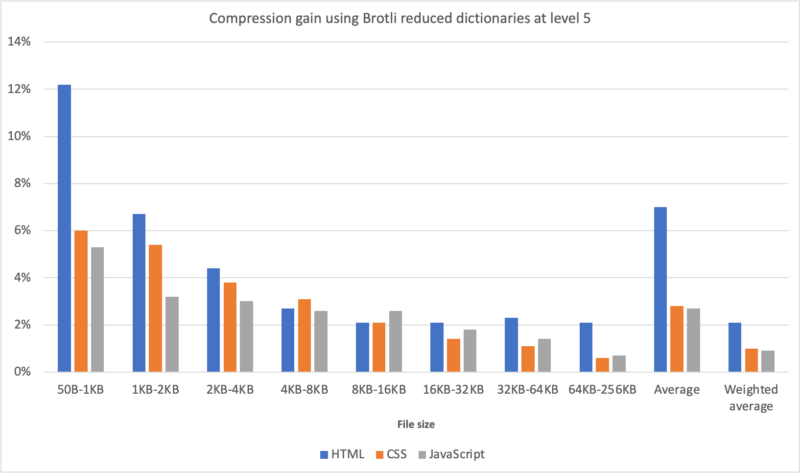
We made our WAF Machine Learning models 5.5x faster, reducing execution time by approximately 82%, from 1519 to 275 microseconds! Read on to find out how we achieved this remarkable improvement.
WAF Attack Score is Cloudflare’s machine learning (ML)-powered layer built on top of our Web Application Firewall (WAF). Its goal is to complement the WAF and detect attack bypasses that we haven’t encountered before. This has proven invaluable in catching zero-day vulnerabilities, like the one detected in Ivanti Connect Secure, before they are publicly disclosed and enhancing our customers’ protection against emerging and unknown threats.
Since its launch in 2022, WAF attack score adoption has grown exponentially, now protecting millions of Internet properties and running real-time inference on tens of millions of requests per second. The feature’s popularity has driven us to seek performance improvements, enabling even broader customer use and enhancing Internet security.
In this post, we will discuss the performance optimizations we’ve implemented for our WAF ML product. We’ll guide you through specific code examples and benchmark numbers, demonstrating how these enhancements have significantly improved our system’s efficiency. Additionally, we’ll share the impressive latency reduction numbers observed after the rollout.
Before diving into the optimizations, let’s take a moment to review the inner workings of the WAF Attack Score, which powers our WAF ML product.
WAF Attack Score system design
Cloudflare’s WAF attack score identifies various traffic types and attack vectors (SQLi, XSS, Command Injection, etc.) based on structural or statistical content properties. Here’s how it works during inference:
HTTP Request Content: Start with raw HTTP input.
Normalization & Transformation: Standardize and clean the data, applying normalization, content substitutions, and de-duplication.
Feature Extraction: Tokenize the transformed content to generate statistical and structural data.
Machine Learning Model Inference: Analyze the extracted features with pre-trained models, mapping content representations to classes (e.g., XSS, SQLi or RCE) or scores.
Classification Output in WAF: Assign a score to the input, ranging from 1 (likely malicious) to 99 (likely clean), guiding security actions.
Next, we will explore feature extraction and inference optimizations.
Feature extraction optimizations
In the context of the WAF Attack Score ML model, feature extraction or pre-processing is essentially a process of tokenizing the given input and producing a float tensor of 1 x m size:
In our initial pre-processing implementation, this is achieved via a sliding window of 3 bytes over the input with the help of Rust’s std::collections::HashMap to look up the tensor index for a given ngram.
Initial benchmarks
To establish performance baselines, we’ve set up four benchmark cases representing example inputs of various lengths, ranging from 44 to 9482 bytes. Each case exemplifies typical input sizes, including those for a request body, user agent, and URI. We run benchmarks using the Criterion.rs statistics-driven micro-benchmarking tool:
Here are initial numbers for these benchmarks executed on a Linux laptop with a 13th Gen Intel® Core™ i7-13800H processor:
Benchmark case
Pre-processing time, μs
Throughput, MiB/s
preprocessing/long-body-9482
248.46
36.40
preprocessing/avg-body-1000
28.19
33.83
preprocessing/avg-url-44
1.45
28.94
preprocessing/avg-ua-91
2.87
30.24
An important observation from these results is that pre-processing time correlates with the length of the input string, with throughput ranging from 28 MiB/s to 36 MiB/s. This suggests that considerable time is spent iterating over longer input strings. Optimizing this part of the process could significantly enhance performance. The dependency of processing time on input size highlights a key area for performance optimization. To validate this, we should examine where the processing time is spent by analyzing flamegraphs created from a 100-second profiling session visualized using pprof:
Looking at the pre-processing flamegraph above, it’s clear that most of the time was spent on the following two operations:
Function name
% Time spent
std::collections::hash::map::HashMap<K,V,S>::get
61.8%
regex::regex::bytes::Regex::replace_all
18.5%
Let’s tackle the HashMap lookups first. Lookups are happening inside the tensor_populate_ngrams function, where input is split into windows of 3 bytes representing ngram and then lookup inside two hash maps:
fn tensor_populate_ngrams(tensor: &mut [f32], input: &[u8]) {
   // Populate the NORM ngrams
   let mut unknown_norm_ngrams = 0;
   let norm_offset = 1;

   for s in input.windows(3) {
       match NORM_VOCAB.get(s) {
           Some(pos) => {
               tensor[*pos as usize + norm_offset] += 1.0f32;
           }
           None => {
               unknown_norm_ngrams += 1;
           }
       };
   }

   // Populate the SIG ngrams
   let mut unknown_sig_ngrams = 0;
   let sig_offset = norm_offset + NORM_VOCAB.len();

   let res = SIG_REGEX.replace_all(&input, b"#");

   for s in res.windows(3) {
       match SIG_VOCAB.get(s) {
           Some(pos) => {
               // adding +1 here as the first position will be the unknown_sig_ngrams
               tensor[*pos as usize + sig_offset + 1] += 1.0f32;
           }
           None => {
               unknown_sig_ngrams += 1;
           }
       }
   }
}
So essentially the pre-processing function performs a ton of hash map lookups, the volume of which depends on the size of the input string, e.g. 1469 lookups for the given benchmark case avg-body-1000.
Optimization attempt #1: HashMap → Aho-Corasick
Rust hash maps are generally quite fast. However, when that many lookups are being performed, it’s not very cache friendly.
So can we do better than hash maps, and what should we try first? The answer is the Aho-Corasick library.
This library provides multiple pattern search principally through an implementation of the Aho-Corasick algorithm, which builds a fast finite state machine for executing searches in linear time.
We can also tune Aho-Corasick settings based on this recommendation:
Then we use the constructed AhoCorasick dictionary to lookup ngrams using its find_overlapping_iter method:
for mat in NORM_VOCAB_AC.find_overlapping_iter(&input) {
    tensor_input_data[mat.pattern().as_usize() + 1] += 1.0;
}
We ran benchmarks and compared them against the baseline times shown above:
Benchmark case
Baseline time, μs
Aho-Corasick time, μs
Optimization
preprocessing/long-body-9482
248.46
129.59
-47.84% or 1.64x
preprocessing/avg-body-1000
28.19
16.47
-41.56% or 1.71x
preprocessing/avg-url-44
1.45
1.01
-30.38% or 1.44x
preprocessing/avg-ua-91
2.87
1.90
-33.60% or 1.51x
That’s substantially better – Aho-Corasick DFA does wonders.
Optimization attempt #2: Aho-Corasick → match
One would think optimization with Aho-Corasick DFA is enough and that it seems unlikely that anything else can beat it. Yet, we can throw Aho-Corasick away and simply use the Rust match statement and let the compiler do the optimization for us!
Here’s how it performs in practice, based on the assembly generated by the Godbolt compiler explorer. The corresponding assembly code efficiently implements this lookup by employing a jump table and byte-wise comparisons to determine the return value based on input sequences, optimizing for quick decisions and minimal branching. Although the example only includes ten ngrams, it’s important to note that in applications like our WAF Attack Score ML models, we deal with thousands of ngrams. This simple match-based approach outshines both HashMap lookups and the Aho-Corasick method.
Benchmark case
Baseline time, μs
Match time, μs
Optimization
preprocessing/long-body-9482
248.46
112.96
-54.54% or 2.20x
preprocessing/avg-body-1000
28.19
13.12
-53.45% or 2.15x
preprocessing/avg-url-44
1.45
0.75
-48.37% or 1.94x
preprocessing/avg-ua-91
2.87
1.4076
-50.91% or 2.04x
Switching to match gave us another 7-18% drop in latency, depending on the case.
Optimization attempt #3: Regex → WindowedReplacer
So, what exactly is the purpose of Regex::replace_all in pre-processing? Regex is defined and used like this:
pub static SIG_REGEX: Lazy<Regex> =
    Lazy::new(|| RegexBuilder::new("[a-z]+").unicode(false).build().unwrap());
    ...
    let res = SIG_REGEX.replace_all(&input, b"#");
    for s in res.windows(3) {
        tensor[sig_vocab_lookup(s.try_into().unwrap())] += 1.0;
    }
Essentially, all we need is to:
Replace every sequence of lowercase letters in the input with a single byte “#”.
Iterate over replaced bytes in a windowed fashion with a step of 3 bytes representing an ngram.
Look up the ngram index and increment it in the tensor.
This logic seems simple enough that we could implement it more efficiently with a single pass over the input and without any allocations:
type Window = [u8; 3];
type Iter<'a> = Peekable<std::slice::Iter<'a, u8>>;

pub struct WindowedReplacer<'a> {
    window: Window,
    input_iter: Iter<'a>,
}

#[inline]
fn is_replaceable(byte: u8) -> bool {
    matches!(byte, b'a'..=b'z')
}

#[inline]
fn next_byte(iter: &mut Iter) -> Option<u8> {
    let byte = iter.next().copied()?;
    if is_replaceable(byte) {
        while iter.next_if(|b| is_replaceable(**b)).is_some() {}
        Some(b'#')
    } else {
        Some(byte)
    }
}

impl<'a> WindowedReplacer<'a> {
    pub fn new(input: &'a [u8]) -> Option<Self> {
        let mut window: Window = Default::default();
        let mut iter = input.iter().peekable();
        for byte in window.iter_mut().skip(1) {
            *byte = next_byte(&mut iter)?;
        }
        Some(WindowedReplacer {
            window,
            input_iter: iter,
        })
    }
}

impl<'a> Iterator for WindowedReplacer<'a> {
    type Item = Window;

    #[inline]
    fn next(&mut self) -> Option<Self::Item> {
        for i in 0..2 {
            self.window[i] = self.window[i + 1];
        }
        let byte = next_byte(&mut self.input_iter)?;
        self.window[2] = byte;
        Some(self.window)
    }
}
By utilizing the WindowedReplacer, we simplify the replacement logic:
if let Some(replacer) = WindowedReplacer::new(&input) {
    for ngram in replacer.windows(3) {
        tensor[sig_vocab_lookup(ngram.try_into().unwrap())] += 1.0;
    }
}
This new approach not only eliminates the need for allocating additional buffers to store replaced content, but also leverages Rust’s iterator optimizations, which the compiler can more effectively optimize. You can view an example of the assembly output for this new iterator at the provided Godbolt link.
Now let’s benchmark this and compare against the original implementation:
Benchmark case
Baseline time, μs
Match time, μs
Optimization
preprocessing/long-body-9482
248.46
51.00
-79.47% or 4.87x
preprocessing/avg-body-1000
28.19
5.53
-80.36% or 5.09x
preprocessing/avg-url-44
1.45
0.40
-72.11% or 3.59x
preprocessing/avg-ua-91
2.87
0.69
-76.07% or 4.18x
The new letters replacement implementation has doubled the preprocessing speed compared to the previously optimized version using match statements, and it is four to five times faster than the original version!
Optimization attempt #4: Going nuclear with branchless ngram lookups
At this point, 4-5x improvement might seem like a lot and there is no point pursuing any further optimizations. After all, using an ngram lookup with a match statement has beaten the following methods, with benchmarks omitted for brevity:
A Rust crate that allows you to use static compile-time generated hash maps and hash sets using PTHash perfect hash functions.
However, if we look again at the assembly of the norm_vocab_lookup function, it is clear that the execution flow has to perform a bunch of comparisons using cmp instructions. This creates many branches for the CPU to handle, which can lead to branch mispredictions. Branch mispredictions occur when the CPU incorrectly guesses the path of execution, causing delays as it discards partially completed instructions and fetches the correct ones. By reducing or eliminating these branches, we can avoid these mispredictions and improve the efficiency of the lookup process. How can we get rid of those branches when there is a need to look up thousands of unique ngrams?
Since there are only 3 bytes in each ngram, we can build two lookup tables of 256 x 256 x 256 size, storing the ngram tensor index. With this naive approach, our memory requirements will be: 256 x 256 x 256 x 2 x 2 = 64 MB, which seems like a lot.
However, given that we only care about ASCII bytes 0..127, then memory requirements can be lower: 128 x 128 x 128 x 2 x 2 = 8 MB, which is better. However, we will need to check for bytes >= 128, which will introduce a branch again.
So can we do better? Considering that the actual number of distinct byte values used in the ngrams is significantly less than the total possible 256 values, we can reduce memory requirements further by employing the following technique:
1. To avoid the branching caused by comparisons, we use precomputed offset lookup tables. This means instead of comparing each byte of the ngram during each lookup, we precompute the positions of each possible byte in a lookup table. This way, we replace the comparison operations with direct memory accesses, which are much faster and do not involve branching. We build an ngram bytes offsets lookup const array, storing each unique ngram byte offset position multiplied by the number of unique ngram bytes:
const NGRAM_OFFSETS: [[u32; 256]; 3] = [
    [
        // offsets of first byte in ngram
    ],
    [
        // offsets of second byte in ngram
    ],
    [
        // offsets of third byte in ngram
    ],
];
2. Then to obtain the ngram index, we can use this simple const function:
#[inline]
const fn ngram_index(ngram: [u8; 3]) -> usize {
    (NGRAM_OFFSETS[0][ngram[0] as usize]
        + NGRAM_OFFSETS[1][ngram[1] as usize]
        + NGRAM_OFFSETS[2][ngram[2] as usize]) as usize
}
3. To look up the tensor index based on the ngram index, we construct another const array at compile time using a list of all ngrams, where N is the number of unique ngram bytes:
4. Finally, to update the tensor based on given ngram, we lookup the ngram index, then the tensor index, and then increment it with help of get_unchecked_mut, which avoids unnecessary (in this case) boundary checks and eliminates another source of branching:
This logic works effectively, passes correctness tests, and most importantly, it’s completely branchless! Moreover, the memory footprint of used lookup arrays is tiny – just ~500 KiB of memory – which easily fits into modern CPU L2/L3 caches, ensuring that expensive cache misses are rare and performance is optimal.
The last trick we will employ is loop unrolling for ngrams processing. By taking 6 ngrams (corresponding to 8 bytes of the input array) at a time, the compiler can unroll the second loop and auto-vectorize it, leveraging parallel execution to improve performance:
const CHUNK_SIZE: usize = 6;

let chunks_max_offset =
    ((input.len().saturating_sub(2)) / CHUNK_SIZE) * CHUNK_SIZE;
for i in (0..chunks_max_offset).step_by(CHUNK_SIZE) {
    for ngram in input[i..i + CHUNK_SIZE + 2].windows(3) {
        update_tensor_with_ngram(tensor, ngram.try_into().unwrap());
    }
}
Tying up everything together, our final pre-processing benchmarks show the following:
Benchmark case
Baseline time, μs
Branchless time, μs
Optimization
preprocessing/long-body-9482
248.46
21.53
-91.33% or 11.54x
preprocessing/avg-body-1000
28.19
2.33
-91.73% or 12.09x
preprocessing/avg-url-44
1.45
0.26
-82.34% or 5.66x
preprocessing/avg-ua-91
2.87
0.43
-84.92% or 6.63x
The longer input is, the higher the latency drop will be due to branchless ngram lookups and loop unrolling, ranging from six to twelve times faster than baseline implementation.
After trying various optimizations, the final version of pre-processing retains optimization attempts 3 and 4, using branchless ngram lookup with offset tables and a single-pass non-allocating replacement iterator.
There are potentially more CPU cycles left on the table, and techniques like memory pre-fetching and manual SIMD intrinsics could speed this up a bit further. However, let’s now switch gears into looking at inference latency a bit closer.
Model inference optimizations
Initial benchmarks
Let’s have a look at original performance numbers of the WAF Attack Score ML model, which uses TensorFlow Lite 2.6.0:
Benchmark case
Inference time, μs
inference/long-body-9482
247.31
inference/avg-body-1000
246.31
inference/avg-url-44
246.40
inference/avg-ua-91
246.88
Model inference is actually independent of the original input length, as inputs are transformed into tensors of predetermined size during the pre-processing phase, which we optimized above. From now on, we will refer to a singular inference time when benchmarking our optimizations.
Digging deeper with profiler, we observed that most of the time is spent on the following operations:
The most expensive operation is matrix multiplication, which boils down to iteration within three nested loops:
void PortableMatrixBatchVectorMultiplyAccumulate(const float* matrix,
                                                 int m_rows, int m_cols,
                                                 const float* vector,
                                                 int n_batch, float* result) {
  float* result_in_batch = result;
  for (int b = 0; b < n_batch; b++) {
    const float* matrix_ptr = matrix;
    for (int r = 0; r < m_rows; r++) {
      float dot_prod = 0.0f;
      const float* vector_in_batch = vector + b * m_cols;
      for (int c = 0; c < m_cols; c++) {
        dot_prod += *matrix_ptr++ * *vector_in_batch++;
      }
      *result_in_batch += dot_prod;
     ++result_in_batch;
    }
  }
}
This doesn’t look very efficient and many blogs and research papers have been written on how matrix multiplication can be optimized, which basically boils down to:
Blocking: Divide matrices into smaller blocks that fit into the cache, improving cache reuse and reducing memory access latency.
Vectorization: Use SIMD instructions to process multiple data points in parallel, enhancing efficiency with vector registers.
Loop Unrolling: Reduce loop control overhead and increase parallelism by executing multiple loop iterations simultaneously.
To gain a better understanding of how these techniques work, we recommend watching this video, which brilliantly depicts the process of matrix multiplication:
Tensorflow Lite with AVX2
TensorFlow Lite does, in fact, support SIMD matrix multiplication – we just need to enable it and re-compile the TensorFlow Lite library:
if [[ "$(uname -m)" == x86_64* ]]; then
    # On x86_64 target x86-64-v3 CPU to enable AVX2 and FMA.
    arguments+=("--copt=-march=x86-64-v3")
fi
After running profiler again using the SIMD-optimized TensorFlow Lite library:
Matrix multiplication now uses AVX2 instructions, which uses blocks of 8×8 to multiply and accumulate the multiplication result.
Proportionally, matrix multiplication and quantization operations take a similar time share when compared to non-SIMD version, however in absolute numbers, it’s almost twice as fast when SIMD optimizations are enabled:
Benchmark case
Baseline time, μs
SIMD time, μs
Optimization
inference/avg-body-1000
246.31
130.07
-47.19% or 1.89x
Quite a nice performance boost just from a few lines of build config change!
Tensorflow Lite with XNNPACK
Tensorflow Lite comes with a useful benchmarking tool called benchmark_model, which also has a built-in profiler.
Tensorflow Lite with XNNPACK enabled emerges as a leader, achieving ~50% latency reduction, when compared to the original Tensorflow Lite implementation.
More technical details about XNNPACK can be found in these blog posts:
Re-running benchmarks with XNNPack enabled, we get the following results:
Benchmark case
Baseline time, μs TFLite 2.6.0
SIMD time, μs TFLite 2.6.0
SIMD time, μs TFLite 2.16.1
SIMD + XNNPack time, μs TFLite 2.16.1
Optimization
inference/avg-body-1000
246.31
130.07
115.17
56.22
-77.17% or 4.38x
By upgrading TensorFlow Lite from 2.6.0 to 2.16.1 and enabling SIMD optimizations along with the XNNPack, we were able to decrease WAF ML model inference time more than four-fold, achieving a 77.17% reduction.
Caching inference result
While making code faster through pre-processing and inference optimizations is great, it’s even better when code doesn’t need to run at all. This is where caching comes in. Amdahl’s Law suggests that optimizing only parts of a program has diminishing returns. By avoiding redundant executions with caching, we can achieve significant performance gains beyond the limitations of traditional code optimization.
A simple key-value cache would quickly occupy all available memory on the server due to the high cardinality of URLs, HTTP headers, and HTTP bodies. However, because “everything on the Internet has an L-shape” or more specifically, follows a Zipf’s law distribution, we can optimize our caching strategy.
Zipf‘s law states that in many natural datasets, the frequency of any item is inversely proportional to its rank in the frequency table. In other words, a few items are extremely common, while the majority are rare. By analyzing our request data, we found that URLs, HTTP headers, and even HTTP bodies follow this distribution. For example, here is the user agent header frequency distribution against its rank:
By caching the top-N most frequently occurring inputs and their corresponding inference results, we can ensure that both pre-processing and inference are skipped for the majority of requests. This is where the Least Recently Used (LRU) cache comes in – frequently used items stay hot in the cache, while the least recently used ones are evicted.
We use lua-resty-mlcache as our caching solution, allowing us to share cached inference results between different Nginx workers via a shared memory dictionary. The LRU cache effectively exploits the space-time trade-off, where we trade a small amount of memory for significant CPU time savings.
This approach enables us to achieve a ~70% cache hit ratio, significantly reducing latency further, as we will analyze in the final section below.
Optimization results
The optimizations discussed in this post were rolled out in several phases to ensure system correctness and stability.
First, we enabled SIMD optimizations for TensorFlow Lite, which reduced WAF ML total execution time by approximately 41.80%, decreasing from 1519 ➔ 884 μs on average.
Next, we upgraded TensorFlow Lite from version 2.6.0 to 2.16.1, enabled XNNPack, and implemented pre-processing optimizations. This further reduced WAF ML total execution time by ~40.77%, bringing it down from 932 ➔ 552 μs on average. The initial average time of 932 μs was slightly higher than the previous 884 μs due to the increased number of customers using this feature and the months that passed between changes.
Lastly, we introduced LRU caching, which led to an additional reduction in WAF ML total execution time by ~50.18%, from 552 ➔ 275 μs on average.
Overall, we cut WAF ML execution time by ~81.90%, decreasing from 1519 ➔ 275 μs, or 5.5x faster!
To illustrate the significance of this: with Cloudflare’s average rate of 9.5 million requests per second passing through WAF ML, saving 1244 microseconds per request equates to saving ~32 years of processing time every single day! That’s in addition to the savings of 523 microseconds per request or 65 years of processing time per day demonstrated last year in our Every request, every microsecond: scalable machine learning at Cloudflare post about our Bot Management product.
Conclusion
We hope you enjoyed reading about how we made our WAF ML models go brrr, just as much as we enjoyed implementing these optimizations to bring scalable WAF ML to more customers on a truly global scale.
Looking ahead, we are developing even more sophisticated ML security models. These advancements aim to bring our WAF and Bot Management products to the next level, making them even more useful and effective for our customers.
AWS Glue is a fully managed, serverless data integration service provided by Amazon Web Services (AWS) that uses Apache Spark as one of its backend processing engines (as of this writing, you can use Python Shell, Spark, or Ray).
Data skew occurs when the data being processed is not evenly distributed across the Spark cluster, causing some tasks to take significantly longer to complete than others. This can lead to inefficient resource utilization, longer processing times, and ultimately, slower performance. Data skew can arise from various factors, including uneven data distribution, skewed join keys, or uneven data processing patterns. Even though the biggest issue is often having nodes running out of disk during shuffling, which leads to nodes falling like dominoes and job failures, it’s also important to mention that data skew is hidden. The stealthy nature of data skew means it can often go undetected because monitoring tools might not flag an uneven distribution as a critical issue, and logs don’t always make it evident. As a result, a developer may observe that their AWS Glue jobs are completing without apparent errors, yet the system could be operating far from its optimal efficiency. This hidden inefficiency not only increases operational costs due to longer runtimes but can also lead to unpredictable performance issues that are difficult to diagnose without a deep dive into the data distribution and task run patterns.
For example, in a dataset of customer transactions, if one customer has significantly more transactions than the others, it can cause a skew in the data distribution.
Identifying and handling data skew issues is key to having good performance on Apache Spark and therefore on AWS Glue jobs that use Spark as a backend. In this post, we show how you can identify data skew and discuss the different techniques to mitigate data skew.
How to detect data skew
When an AWS Glue job has issues with local disks (split disk issues), doesn’t scale with the number of workers, or has low CPU usage (you can enable Amazon CloudWatch metrics for your job to be able to see this), you may have a data skew issue. You can detect data skew with data analysis or by using the Spark UI. In this section, we discuss how to use the Spark UI.
The Spark UI provides a comprehensive view of Spark applications, including the number of tasks, stages, and their duration. To use it you need to enable Spark UI event logs for your job runs. It is enabled by default on Glue console and once enabled, Spark event log files will be created during the job run and stored in your S3 bucket. Then, those logs are parsed, and you can use the AWS Glue serverless Spark UI to visualize them. You can refer to this blogpost for more details. In those jobs where the AWS Glue serverless Spark UI does not work as it has a limit of 512 MB of logs, you can set up the Spark UI using an EC2 instance.
You can use the Spark UI to identify which tasks are taking longer to complete than others, and if the data distribution among partitions is balanced or not (remember that in Spark, one partition is mapped to one task). If there is data skew, you will see that some partitions have significantly more data than others. The following figure shows an example of this. We can see that one task is taking a lot more time than the others, which can indicate data skew.
Another thing that you can use is the summary metrics for each stage. The following screenshot shows another example of data skew.
These metrics represent the task-related metrics below which a certain percentage of tasks completed. For example, the 75th percentile task duration indicates that 75% of tasks completed in less time than this value. When the tasks are evenly distributed, you will see similar numbers in all the percentiles. When there is data skew, you will see very biased values in each percentile. In the preceding example, it didn’t write many shuffle files (less than 50 MiB) in Min, 25th percentile, Median, and 75th percentile. However, in Max, it wrote 460 MiB, 10 times the 75th percentile. It means there was at least one task (or up to 25% of tasks) that wrote much bigger shuffle files than the rest of the tasks. You can also see that the duration of the tax in Max is 46 seconds and the Median is 2 seconds. These are all indicators that your dataset may have data skew.
AWS Glue interactive sessions
You can use interactive sessions to load your data from the AWS Glue Data Catalog or just use Spark methods to load the files such as Parquet or CSV that you want to analyze. You can use a similar script to the following to detect data skew from the partition size perspective; the more important issue is related to data skew while shuffling, and this script does not detect that kind of skew:
from pyspark.sql.functions import spark_partition_id, asc, desc
#input_dataframe being the dataframe where you want to check for data skew
partition_sizes_df=input_dataframe\
    .withColumn("partitionId", spark_partition_id())\
    .groupBy("partitionId")\
    .count()\
    .orderBy(asc("count"))\
    .withColumnRenamed("count","partition_size")
#calculate average and standar deviation for the partition sizes
avg_size = partition_sizes_df.agg({"partition_size": "avg"}).collect()[0][0]
std_dev_size = partition_sizes_df.agg({"partition_size": "stddev"}).collect()[0][0]

"""
 the code calculates the absolute difference between each value in the "partition_size" column and the calculated average (avg_size).
 then, calculates twice the standard deviation (std_dev_size) and use
 that as a boolean mask where the condition checks if the absolute difference is greater than twice the standard deviation
 in order to mark a partition 'skewed'
"""
skewed_partitions_df = partition_sizes_df.filter(abs(partition_sizes_df["partition_size"] - avg_size) > 2 * std_dev_size)
if skewed_partitions_df.count() > 0:
    skewed_partitions = [row["partition_id"] for row in skewed_partitions_df.collect()]
    print(f"The following partitions have significantly different sizes: {skewed_partitions}")
else:
    print("No data skew detected.")
You can calculate the average and standard deviation of partition sizes using the agg() function and identify partitions with significantly different sizes using the filter() function, and you can print their indexes if any skewed partitions are detected. Otherwise, the output prints that no data skew is detected.
This code assumes that your data is structured, and you may need to modify it if your data is of a different type.
How to handle data skew
You can use different techniques in AWS Glue to handle data skew; there is no single universal solution. The first thing to do is confirm that you’re using latest AWS Glue version, for example AWS Glue 4.0 based on Spark 3.3 has enabled by default some configs like Adaptative Query Execution (AQE) that can help improve performance when data skew is present.
The following are some of the techniques that you can employ to handle data skew:
Filter and perform – If you know which keys are causing the skew, you can filter them out, perform your operations on the non-skewed data, and then handle the skewed keys separately.
Implementing incremental aggregation – If you are performing a large aggregation operation, you can break it up into smaller stages because in large datasets, a single aggregation operation (like sum, average, or count) can be resource-intensive. In those cases, you can perform intermediate actions. This could involve filtering, grouping, or additional aggregations. This can help distribute the workload across the nodes and reduce the size of intermediate data.
Using a custom partitioner – If your data has a specific structure or distribution, you can create a custom partitioner that partitions your data based on its characteristics. This can help make sure that data with similar characteristics is in the same partition and reduce the size of the largest partition.
Using broadcast join – If your dataset is small but exceeds the spark.sql.autoBroadcastJoinThreshold value (default is 10 MB), you have the option to either provide a hint to use broadcast join or adjust the threshold value to accommodate your dataset. This can be an effective strategy to optimize join operations and mitigate data skew issues resulting from shuffling large amounts of data across nodes.
Salting – This involves adding a random prefix to the key of skewed data. By doing this, you distribute the data more evenly across the partitions. After processing, you can remove the prefix to get the original key values.
These are just a few techniques to handle data skew in PySpark; the best approach will depend on the characteristics of your data and the operations you are performing.
The following is an example of joining skewed data with the salting technique:
from pyspark.sql import SparkSession
from pyspark.sql.functions import lit, ceil, rand, concat, col

# Define the number of salt values
num_salts = 3

# Function to identify skewed keys
def identify_skewed_keys(df, key_column, threshold):
    key_counts = df.groupBy(key_column).count()
    return key_counts.filter(key_counts['count'] > threshold).select(key_column)

# Identify skewed keys
skewed_keys = identify_skewed_keys(skewed_data, "key", skew_threshold)

# Splitting the dataset
skewed_data_subset = skewed_data.join(skewed_keys, ["key"], "inner")
non_skewed_data_subset = skewed_data.join(skewed_keys, ["key"], "left_anti")

# Apply salting to skewed data
skewed_data_subset = skewed_data_subset.withColumn("salt", ceil((rand() * 10) % num_salts))
skewed_data_subset = skewed_data_subset.withColumn("salted_key", concat(col("key"), lit("_"), col("salt")))

# Replicate skewed rows in non-skewed dataset
def replicate_skewed_rows(df, keys, multiplier):
    replicated_df = df.join(keys, ["key"]).crossJoin(spark.range(multiplier).withColumnRenamed("id", "salt"))
    replicated_df = replicated_df.withColumn("salted_key", concat(col("key"), lit("_"), col("salt")))
    return replicated_df.drop("salt")

replicated_non_skewed_data = replicate_skewed_rows(non_skewed_data, skewed_keys, num_salts)

# Perform the JOIN operation on the salted keys for skewed data
result_skewed = skewed_data_subset.join(replicated_non_skewed_data, "salted_key")

# Perform regular join on non-skewed data
result_non_skewed = non_skewed_data_subset.join(non_skewed_data, "key")

# Combine results
final_result = result_skewed.union(result_non_skewed)
In this code, we first define a salt value, which can be a random integer or any other value. We then add a salt column to our DataFrame using the withColumn() function, where we set the value of the salt column to a random number using the rand() function with a fixed seed. The function replicate_salt_rows is defined to replicate each row in the non-skewed dataset (non_skewed_data) num_salts times. This ensures that each key in the non-skewed data has matching salted keys. Finally, a join operation is performed on the salted_key column between the skewed and non-skewed datasets. This join is more balanced compared to a direct join on the original key, because salting and replication have mitigated the data skew.
The rand() function used in this example generates a random number between 0–1 for each row, so it’s important to use a fixed seed to achieve consistent results across different runs of the code. You can choose any fixed integer value for the seed.
The following figures illustrate the data distribution before (left) and after (right) salting. Heavily skewed key2 identified and salted into key2_0, key2_1, and key2_2, balancing the data distribution and preventing any single node from being overloaded. After processing, the results can be aggregated back, so that that the final output is consistent with the unsalted key values.
Other techniques to use on skewed data during the join operation
When you’re performing skewed joins, you can use salting or broadcasting techniques, or divide your data into skewed and regular parts before joining the regular data and broadcasting the skewed data.
If you are using Spark 3, there are automatic optimizations for trying to optimize Data Skew issues on joins. Those can be tuned because they have dedicated configs on Apache Spark.
Conclusion
This post provided details on how to detect data skew in your data integration jobs using AWS Glue and different techniques for handling it. Having a good data distribution is key to achieving the best performance on distributed processing systems like Apache Spark.
Although this post focused on AWS Glue, the same concepts apply to jobs you may be running on Amazon EMR using Apache Spark or Amazon Athena for Apache Spark.
As always, AWS welcomes your feedback. Please leave your comments and questions in the comments section.
About the Authors
Salim Tutuncu is a Sr. PSA Specialist on Data & AI, based from Amsterdam with a focus on the EMEA North and EMEA Central regions. With a rich background in the technology sector that spans roles as a Data Engineer, Data Scientist, and Machine Learning Engineer, Salim has built a formidable expertise in navigating the complex landscape of data and artificial intelligence. His current role involves working closely with partners to develop long-term, profitable businesses leveraging the AWS Platform, particularly in Data and AI use cases.
Angel Conde Manjon is a Sr. PSA Specialist on Data & AI, based in Madrid, and focuses on EMEA South and Israel. He has previously worked on research related to Data Analytics and Artificial Intelligence in diverse European research projects. In his current role, Angel helps partners develop businesses centered on Data and AI.
Distributed applications resiliency is a cumulative resiliency of applications, infrastructure, and operational processes. Part 1 of this series explored application layer resiliency. In Part 2, we discuss how using Amazon Web Services (AWS) managed services, redundancy, high availability, and infrastructure failover patterns based on recovery time and point objectives (RTO and RPO, respectively) can help in building more resilient infrastructures.
Pattern 1: Recognize high impact/likelihood infrastructure failures
To ensure cloud infrastructure resilience, we need to understand the likelihood and impact of various infrastructure failures, so we can mitigate them. Figure 1 illustrates that most of the failures with high likelihood happen because of operator error or poor deployments.
Automated testing, automated deployments, and solid design patterns can mitigate these failures. There could be datacenter failures—like whole rack failures—but deploying applications using auto scaling and multi-availability zone (multi-AZ) deployment, plus resilient AWS cloud native services, can mitigate the impact.
Figure 1. Likelihood and impact of failure events
As demonstrated in the Figure 1, infrastructure resiliency is a combination of high availability (HA) and disaster recovery (DR). HA involves increasing the availability of the system by implementing redundancy among the application components and removing single points of failure.
Application layer decisions, like creating stateless applications, make it simpler to implement HA at the infrastructure layer by allowing it to scale using Auto Scaling groups and distributing the redundant applications across multiple AZs.
Pattern 2: Understanding and controlling infrastructure failures
Building a resilient infrastructure requires understanding which infrastructure failures are under control and which ones are not, as demonstrated in Figure 2.
These insights allow us to automate the detection of failures, control them, and employ pro-active patterns, such as static stability, to mitigate the need to scale up the infrastructure by over-provisioning it in advance.
Figure 2. Proactively designing systems in the event of failure
The infrastructure decisions under our control that can increase the infrastructure resiliency of our system, include:
AWS services have control and data planes designed for minimum blast radius. Data planes typically have higher availability design goals than control planes and are usually less complex. When implementing recovery or mitigation responses to events that can affect resiliency, using control plane operations can lower the overall resiliency of your architectures. For example, Amazon Route 53 (Route 53) has a data plane designed for a 100% availability SLA. A good fail-over mechanism should rely on the data plane and not the control plane, as explained in Creating Disaster Recovery Mechanisms Using Amazon Route 53.
Understanding networking design and routes implemented in a virtual private cloud (VPC) are critical when testing the flow of traffic in our application. Understanding the flow of traffic helps us design better applications and see how one component failure can affect overall ingress/egress traffic. To achieve better network resiliency, it’s important to implement a good subnet strategy and manage our IP addresses to avoid fail-over issues and asymmetric routing in hybrid architectures. Use IP address management tools for established subnet strategies and routing decisions.
When designing VPCs and AZs, understanding the service limits, deploying independent routing tables and components in each zone increases availability. For example, highly available NAT gateways are preferred over NAT instances, as noted in the comparison provided in the Amazon VPC documentation.
Pattern 3: Considering different ways of increasing HA at the infrastructure layer
As already detailed, infrastructure resiliency = HA + DR.
Different ways by which system availability can be increased include:
Building for redundancy: Redundancy is the duplication of application components to increase the overall availability of the distributed system. After following application layer best practices, we can build auto healing mechanisms at the infrastructure layer.
We can take advantage of auto scaling features and use Amazon CloudWatch metrics and alarms to set up auto scaling triggers and deploy redundant copies of our applications across multiple AZs. This protects workloads from AZ failures, as shown in Figure 3.
Figure 3. Redundancy increases availability
Auto scale your infrastructure: When there are AZ failures, infrastructure auto scaling maintains the desired number of redundant components, which helps maintain the base level application throughput. This way, HA system and manage costs are maintained. Auto scaling uses metrics to scale in and out, appropriately, as shown in Figure 4.
Figure 4. How auto scaling improves availability
Implement resilient network connectivity patterns: While building highly resilient distributed systems, network access to AWS infrastructure also needs to be highly resilient. While deploying hybrid applications, the capacity needed for hybrid applications to communicate with their cloud native application counterparts is an important consideration in designing the network access using AWS Direct Connect or VPNs.
Testing failover and fallback scenarios helps validate that network paths operate as expected and routes fail over as expected to meet RTO objectives. As the number of connection points between the data center and AWS VPCs increases, a hub and spoke configuration provided by the Direct Connect gateway and transit gateways simplify network topology, testing, and fail over. For more information, visit the AWS Direct Connect Resiliency Recommendations.
Whenever possible, use the AWS networking backbone to increase security, resiliency, and lower cost. AWS PrivateLink provides secure access to AWS services and exposes the application’s functionalities and APIs to other business units or partner accounts hosted on AWS.
Think ahead about DNS resolution: DNS is a critical infrastructure component; hybrid DNS resolution should be designed carefully with Route 53 HA inbound and outbound resolver endpoints instead of using self-managed proxies.
Implement a good strategy to share DNS resolver rules across AWS accounts and VPC’s with Resource Access Manager. Network failover tests are an important part of Disaster Recovery and Business Continuity Plans. To learn more, visit Set up integrated DNS resolution for hybrid networks in Amazon Route 53.
Additionally, ELB uses health checks to make sure that requests will route to another component if the underlying traffic application component fails. This improves the distributed system’s availability, as it is the cumulative availability of all different layers in our system. Figure 5 details advantages of some AWS managed services.
Figure 5. AWS managed services help in building resilient infrastructures (click the image to enlarge)
Pattern 4: Use RTO and RPO requirements to determine the correct failover strategy for your application
Capture RTO and RPO requirements early on to determine solid failover strategies (Figure 6). Disaster recovery strategies within AWS range from low cost and complexity (like backup and restore), to more complex strategies when lower values of RTO and RPO are required.
In pilot light and warm standby, only the primary region receives traffic. Pilot light only critical infrastructure components run in the backup region. Automation is used to check failures in the primary region using health checks and other metrics.
When health checks fail, use a combination of auto scaling groups, automation, and Infrastructure as Code (IaC) for quick deployment of other infrastructure components.
Note: This strategy depends on control plane availability in the secondary region for deploying the resources; keep this point in mind if you don’t have compute pre-provisioned in the secondary region. Carefully consider the business requirements and a distributed system’s application-level characteristics before deciding on a failover strategy. To understand all the factors and complexities involved in each of these disaster recovery strategies refer to disaster recovery options in the cloud.
Figure 6. Relationship between RTO, RPO, cost, data loss, and length of service interruption
Conclusion
In Part 2 of this series, we discovered that infrastructure resiliency is a combination of HA and DR. It is important to consider likelihood and impact of different failure events on availability requirements. Building in application layer resiliency patterns (Part 1 of this series), along with early discovery of the RTO/RPO requirements, as well as operational and process resiliency of an organization helps in choosing the right managed services and putting in place the appropriate failover strategies for distributed systems.
It’s important to differentiate between normal and abnormal load threshold for applications in order to put automation, alerts, and alarms in place. This allows us to auto scale our infrastructure for normal expected load, plus implement corrective action and automation to root out issues in case of abnormal load. Use IaC for quick failover and test failover processes.
Stay tuned for Part 3, in which we discuss operational resiliency!
Amazon Redshift is a fully managed, petabyte-scale, massively parallel data warehouse that offers simple operations and high performance. It makes it fast, simple, and cost-effective to analyze all your data using standard SQL and your existing business intelligence (BI) tools. Today, Amazon Redshift has become the most widely used cloud data warehouse.
RA3 nodes – Amazon Redshift RA3 nodes are backed by a new managed storage model that gives you the power to separately optimize your compute power and your storage. They bring a few very important features, one of which is data sharing. RA3 nodes also support the ability to pause and resume, which allows you to easily suspend on-demand billing while the cluster is not being used.
Data sharing – Amazon Redshift data sharing offers you to extend the ease of use, performance, and cost benefits of Amazon Redshift in a single cluster to multi-cluster deployments while being able to share data. Data sharing enables instant, granular, and fast data access across Redshift clusters without the need to copy or move it. You can securely share live data with Amazon Redshift clusters in the same or different AWS accounts, and across regions. You can share data at many levels, including schemas, tables, views, and user-defined functions. You can also share the most up-to-date and consistent information as it’s updated in Amazon Redshift Serverless. It also provides fine-grained access controls that you can tailor for different users and businesses that all need access to the data. However, data sharing in Amazon Redshift has a few limitations.
Solution overview
In this use case, our customer is heavily using Amazon Redshift as their data warehouse for their analytics workloads, and they have been enjoying the possibility and convenience that Amazon Redshift brought to their business. They mainly use Amazon Redshift to store and process user behavioral data for BI purposes. The data has increased by hundreds of gigabytes daily in recent months, and employees from departments continuously run queries against the Amazon Redshift cluster on their BI platform during business hours.
The company runs four major analytics workloads on a single Amazon Redshift cluster, because some data is used by all workloads:
Queries from the BI platform – Various queries run mainly during business hours.
Hourly ETL – This extract, transform, and load (ETL) job runs in the first few minutes of each hour. It generally takes about 40 minutes.
Daily ETL – This job runs twice a day during business hours, because the operation team needs to get daily reports before the end of the day. Each job normally takes between 1.5–3 hours. It’s the second-most resource-heavy workload.
Weekly ETL – This job runs in the early morning every Sunday. It’s the most resource-heavy workload. The job normally takes 3–4 hours.
The analytics team has migrated to the RA3 family and increased the number of nodes of the Amazon Redshift cluster to 12 over the years to keep the average runtime of queries from their BI tool within an acceptable time due to the data size, especially when other workloads are running.
However, they have noticed that performance is reduced while running ETL tasks, and the duration of ETL tasks is long. Therefore, the analytics team wants to explore solutions to optimize their Amazon Redshift cluster.
Because CPU utilization spikes appear while the ETL tasks are running, the AWS team’s first thought was to separate workloads and relevant data into multiple Amazon Redshift clusters with different cluster sizes. By reducing the total number of nodes, we hoped to reduce the cost of Amazon Redshift.
After a series of conversations, the AWS team found that one of the reasons that the customer keeps all workloads on the 12-node Amazon Redshift cluster is to manage the performance of queries from their BI platform, especially while running ETL workloads, which have a big impact on the performance of all workloads on the Amazon Redshift cluster. The obstacle is that many tables in the data warehouse are required to be read and written by multiple workloads, and only the producer of a data share can update the shared data.
The challenge of dividing the Amazon Redshift cluster into multiple clusters is data consistency. Some tables need to be read by ETL workloads and written by BI workloads, and some tables are the opposite. Therefore, if we duplicate data into two Amazon Redshift clusters or only create a data share from the BI cluster to the reporting cluster, the customer will have to develop a data synchronization process to keep the data consistent between all Amazon Redshift clusters, and this process could be very complicated and unmaintainable.
After more analysis to gain an in-depth understanding of the customer’s workloads, the AWS team found that we could put tables into four groups, and proposed a multi-cluster, two-way data sharing solution. The purpose of the solution is to divide the workloads into separate Amazon Redshift clusters so that we can use Amazon Redshift to pause and resume clusters for periodic workloads to reduce the Amazon Redshift running costs, because clusters can still access a single copy of data that is required for workloads. The solution should meet the data consistency requirements without building a complicated data synchronization process.
The following diagram illustrates the old architecture (left) compared to the new multi-cluster solution (right).
Dividing workloads and data
Due to the characteristics of the four major workloads, we categorized workloads into two categories: long-running workloads and periodic-running workloads.
The long-running workloads are for the BI platform and hourly ETL jobs. Because the hourly ETL workload requires about 40 minutes to run, the gain is small even if we migrate it to an isolated Amazon Redshift cluster and pause and resume it every hour. Therefore, we leave it with the BI platform.
The periodic-running workloads are the daily and weekly ETL jobs. The daily job generally takes about 1 hour and 40 minutes to 3 hours, and the weekly job generally takes 3–4 hours.
Data sharing plan
The next step is identifying all data (tables) access patterns of each category. We identified four types of tables:
Type 1 – Tables are only read and written by long-running workloads
Type 2 – Tables are read and written by long-running workloads, and are also read by periodic-running workloads
Type 3 – Tables are read and written by periodic-running workloads, and are also read by long-running workloads
Type 4 – Tables are only read and written by periodic-running workloads
Fortunately, there is no table that is required to be written by all workloads. Therefore, we can separate the Amazon Redshift cluster into two Amazon Redshift clusters: one for the long-running workloads, and the other for periodic-running workloads with 20 RA3 nodes.
We created a two-way data share between the long-running cluster and the periodic-running cluster. For type 2 tables, we created a data share on the long-running cluster as the producer and the periodic-running cluster as the consumer. For type 3 tables, we created a data share on the periodic-running cluster as the producer and the long-running cluster as the consumer.
The following diagram illustrates this data sharing configuration.
Build two-way data share across Amazon Redshift clusters
In this section, we walk through the steps to build a two-way data share across Amazon Redshift clusters. First, let’s take a snapshot of the original Amazon Redshift cluster, which became the long-running cluster later.
Now, let’s create a new Amazon Redshift cluster with 20 RA3 nodes for periodic-running workloads. Then we migrate the type 3 and type 4 tables to the periodic-running cluster. Make sure you choose the ra3 node type. (Amazon Redshift Serverless supports data sharing too, and it becomes generally available in July 2022, so it is also an option now.)
Create the long-to-periodic data share
The next step is to create the long-to-periodic data share. Complete the following steps:
On the periodic-running cluster, get the namespace by running the following query:
SELECT current_namespace;
Make sure record the namespace.
On the long-running cluster, we run queries similar to the following:
CREATE DATASHARE ltop_share SET PUBLICACCESSIBLE TRUE;
ALTER DATASHARE ltop_share ADD SCHEMA public_long;
ALTER DATASHARE ltop_share ADD ALL TABLES IN SCHEMA public_long;
GRANT USAGE ON DATASHARE ltop_share TO NAMESPACE '[periodic-running-cluster-namespace]';
We can validate the long-to-periodic data share using the following command:
SHOW datashares;
After we validate the data share, we get the long-running cluster namespace with the following query:
SELECT current-namespace;
Make sure record the namespace.
On the periodic-running cluster, run the following command to load the data from the long-to-periodic data share with the long-running cluster namespace:
CREATE DATABASE ltop FROM DATASHARE ltop_share OF NAMESPACE '[long-running-cluster-namespace]';
Confirm that we have read access to tables in the long-to-periodic data share.
Create the periodic-to-long data share
The next step is to create the periodic-to-long data share. We use the namespaces of the long-running cluster and the periodic-running cluster that we collected in the previous step.
On the periodic-running cluster, run queries similar to the following to create the periodic-to-long data share:
CREATE DATASHARE ptol_share SET PUBLICACCESSIBLE TRUE;
ALTER DATASHARE ptol_share ADD SCHEMA public_periodic;
ALTER DATASHARE ptol_share ADD ALL TABLES IN SCHEMA public_periodic;
GRANT USAGE ON DATASHARE ptol_share TO NAMESPACE '[long-running-cluster-namespace]';
Validate the data share using the following command:
SHOW datashares;
On the long-running cluster, run the following command to load the data from the periodic-to-long data using the periodic-running cluster namespace:
CREATE DATABASE ptol FROM DATASHARE ptol_share OF NAMESPACE '[periodic-running-cluster-namespace]';
Check that we have read access to the tables in the periodic-to-long data share.
At this stage, we have separated workloads into two Amazon Redshift clusters and built a two-way data share across two Amazon Redshift clusters.
The next step is updating the code of different workloads to use the correct endpoints of two Amazon Redshift clusters and perform consolidated tests.
Pause and resume the periodic-running Amazon Redshift cluster
Let’s update the crontab scripts, which run periodic-running workloads. We make two updates.
When the scripts start, call the Amazon Redshift check and resume cluster APIs to resume the periodic-running Amazon Redshift cluster when the cluster is paused:
After we migrated the workloads to the new architecture, the company’s analytics team ran some tests to verify the results.
According to tests, the performance of all workloads improved:
The BI workload is about 100% faster during the ETL workload running periods
The hourly ETL workload is about 50% faster
The daily workload duration reduced to approximately 40 minutes, from a maximum of 3 hours
The weekly workload duration reduced to approximately 1.5 hours, from a maximum of 4 hours
All functionalities work properly, and cost of the new architecture only increased approximately 13%, while over 10% of new data had been added during the testing period.
Learnings and limitations
After we separated the workloads into different Amazon Redshift clusters, we discovered a few things:
The performance of the BI workloads was 100% faster because there was no resource competition with daily and weekly ETL workloads anymore
The duration of ETL workloads on the periodic-running cluster was reduced significantly because there were more nodes and no resource competition from the BI and hourly ETL workloads
Even when over 10% new data was added, the overall cost of the Amazon Redshift clusters only increased by 13%, due to using the cluster pause and resume function of the Amazon Redshift RA3 family
As a result, we saw a 70% price-performance improvement of the Amazon Redshift cluster.
However, there are some limitations of the solution:
To use the Amazon Redshift pause and resume function, the code for calling the Amazon Redshift pause and resume APIs must be added to all scheduled scripts that run ETL workloads on the periodic-running cluster
Amazon Redshift clusters require several minutes to finish pausing and resuming, although you’re not charged during these processes
The size of Amazon Redshift clusters can’t automatically scale in and out depending on workloads
Next steps
After improving performance significantly, we can explore the possibility of reducing the number of nodes of the long-running cluster to reduce Amazon Redshift costs.
Another possible optimization is using Amazon Redshift Spectrum to reduce the cost of Amazon Redshift on cluster storage. With Redshift Spectrum, multiple Amazon Redshift clusters can concurrently query and retrieve the same structured and semistructured dataset in Amazon Simple Storage Service (Amazon S3) without the need to make copies of the data for each cluster or having to load the data into Amazon Redshift tables.
Amazon Redshift Serverless was announced for preview in AWS re:Invent 2021 and became generally available in July 2022. Redshift Serverless automatically provisions and intelligently scales your data warehouse capacity to deliver best-in-class performance for all your analytics. You only pay for the compute used for the duration of the workloads on a per-second basis. You can benefit from this simplicity without making any changes to your existing analytics and BI applications. You can also share data for read purposes across different Amazon Redshift Serverless instances within or across AWS accounts.
Therefore, we can explore the possibility of removing the need to script for pausing and resuming the periodic-running cluster by using Redshift Serverless to make the management easier. We can also explore the possibility of improving the granularity of workloads.
Conclusion
In this post, we discussed how to optimize workloads on Amazon Redshift clusters using RA3 nodes, data sharing, and pausing and resuming clusters. We also explored a use case implementing a multi-cluster two-way data share solution to improve workload performance with a minimum code change. If you have any questions or feedback, please leave them in the comments section.
About the authors
Jingbin Ma is a Sr. Solutions Architect at Amazon Web Services. He helps customers build well-architected applications using AWS services. He has many years of experience working in the internet industry, and his last role was CTO of a New Zealand IT company before joining AWS. He is passionate about serverless and infrastructure as code.
Chao Pan is a Data Analytics Solutions Architect at Amazon Web Services. He’s responsible for the consultation and design of customers’ big data solution architectures. He has extensive experience in open-source big data. Outside of work, he enjoys hiking.
Here at Cloudflare we’re constantly working on improving our service. Our engineers are looking at hundreds of parameters of our traffic, making sure that we get better all the time.
One of the core numbers we keep a close eye on is HTTP request latency, which is important for many of our products. We regard latency spikes as bugs to be fixed. One example is the 2017 story of “Why does one NGINX worker take all the load?”, where we optimized our TCP Accept queues to improve overall latency of TCP sockets waiting for accept().
Performance tuning is a holistic endeavor, and we monitor and continuously improve a range of other performance metrics as well, including throughput. Sometimes, tradeoffs have to be made. Such a case occurred in 2015, when a latency spike was discovered in our processing of HTTP requests. The solution at the time was to set tcp_rmem to 4 MiB, which minimizes the amount of time the kernel spends on TCP collapse processing. It was this collapse processing that was causing the latency spikes. Later in this post we discuss TCP collapse processing in more detail.
The tradeoff is that using a low value for tcp_rmem limits TCP throughput over high latency links. The following graph shows the maximum throughput as a function of network latency for a window size of 2 MiB. Note that the 2 MiB corresponds to a tcp_rmem value of 4 MiB due to the tcp_adv_win_scale setting in effect at the time.
For the Cloudflare products then in existence, this was not a major problem, as connections terminate and content is served from nearby servers due to our BGP anycast routing.
Since then, we have added new products, such as Magic WAN, WARP, Spectrum, Gateway, and others. These represent new types of use cases and traffic flows.
For example, imagine you’re a typical Magic WAN customer. You have connected all of your worldwide offices together using the Cloudflare global network. While Time to First Byte still matters, Magic WAN office-to-office traffic also needs good throughput. For example, a lot of traffic over these corporate connections will be file sharing using protocols such as SMB. These are elephant flows over long fat networks. Throughput is the metric every eyeball watches as they are downloading files.
We need to continue to provide world-class low latency while simultaneously providing high throughput over high-latency connections.
Before we begin, let’s introduce the players in our game.
TCP receive window is the maximum number of unacknowledged user payload bytes the sender should transmit (bytes-in-flight) at any point in time. The size of the receive window can and does go up and down during the course of a TCP session. It is a mechanism whereby the receiver can tell the sender to stop sending if the sent packets cannot be successfully received because the receive buffers are full. It is this receive window that often limits throughput over high-latency networks.
net.ipv4.tcp_adv_win_scale is a (non-intuitive) number used to account for the overhead needed by Linux to process packets. The receive window is specified in terms of user payload bytes. Linux needs additional memory beyond that to track other data associated with packets it is processing.
The value of the receive window changes during the lifetime of a TCP session, depending on a number of factors. The maximum value that the receive window can be is limited by the amount of free memory available in the receive buffer, according to this table:
tcp_adv_win_scale
TCP window size
4
15/16 * available memory in receive buffer
3
⅞ * available memory in receive buffer
2
¾ * available memory in receive buffer
1
½ * available memory in receive buffer
0
available memory in receive buffer
-1
½ * available memory in receive buffer
-2
¼ * available memory in receive buffer
-3
⅛ * available memory in receive buffer
We can intuitively (and correctly) understand that the amount of available memory in the receive buffer is the difference between the used memory and the maximum limit. But what is the maximum size a receive buffer can be? The answer is sk_rcvbuf.
sk_rcvbuf is a per-socket field that specifies the maximum amount of memory that a receive buffer can allocate. This can be set programmatically with the socket option SO_RCVBUF. This can sometimes be useful to do, for localhost TCP sessions, for example, but in general the use of SO_RCVBUF is not recommended.
So how is sk_rcvbuf set? The most appropriate value for that depends on the latency of the TCP session and other factors. This makes it difficult for L7 applications to know how to set these values correctly, as they will be different for every TCP session. The solution to this problem is Linux autotuning.
Linux autotuning
Linux autotuning is logic in the Linux kernel that adjusts the buffer size limits and the receive window based on actual packet processing. It takes into consideration a number of things including TCP session RTT, L7 read rates, and the amount of available host memory.
Autotuning can sometimes seem mysterious, but it is actually fairly straightforward.
The central idea is that Linux can track the rate at which the local application is reading data off of the receive queue. It also knows the session RTT. Because Linux knows these things, it can automatically increase the buffers and receive window until it reaches the point at which the application layer or network bottleneck links are the constraint on throughput (and not host buffer settings). At the same time, autotuning prevents slow local readers from having excessively large receive queues. The way autotuning does that is by limiting the receive window and its corresponding receive buffer to an appropriate size for each socket.
The values set by autotuning can be seen via the Linux “ss” command from the iproute package (e.g. “ss -tmi”). The relevant output fields from that command are:
Recv-Q is the number of user payload bytes not yet read by the local application.
rcv_ssthresh is the window clamp, a.k.a. the maximum receive window size. This value is not known to the sender. The sender receives only the current window size, via the TCP header field. A closely-related field in the kernel, tp->window_clamp, is the maximum window size allowable based on the amount of available memory. rcv_sshthresh is the receiver-side slow-start threshold value.
skmem_r is the actual amount of memory that is allocated, which includes not only user payload (Recv-Q) but also additional memory needed by Linux to process the packet (packet metadata). This is known within the kernel as sk_rmem_alloc.
Note that there are other buffers associated with a socket, so skmem_r does not represent the total memory that a socket might have allocated. Those other buffers are not involved in the issues presented in this post.
skmem_rb is the maximum amount of memory that could be allocated by the socket for the receive buffer. This is higher than rcv_ssthresh to account for memory needed for packet processing that is not packet data. Autotuning can increase this value (up to tcp_rmem max) based on how fast the L7 application is able to read data from the socket and the RTT of the session. This is known within the kernel as sk_rcvbuf.
rcv_space is the high water mark of the rate of the local application reading from the receive buffer during any RTT. This is used internally within the kernel to adjust sk_rcvbuf.
Earlier we mentioned a setting called tcp_rmem. net.ipv4.tcp_rmem consists of three values, but in this document we are always referring to the third value (except where noted). It is a global setting that specifies the maximum amount of memory that any TCP receive buffer can allocate, i.e. the maximum permissible value that autotuning can use for sk_rcvbuf. This is essentially just a failsafe for autotuning, and under normal circumstances should play only a minor role in TCP memory management.
It’s worth mentioning that receive buffer memory is not preallocated. Memory is allocated based on actual packets arriving and sitting in the receive queue. It’s also important to realize that filling up a receive queue is not one of the criteria that autotuning uses to increase sk_rcvbuf. Indeed, preventing this type of excessive buffering (bufferbloat) is one of the benefits of autotuning.
What’s the problem?
The problem is that we must have a large TCP receive window for high BDP sessions. This is directly at odds with the latency spike problem mentioned above.
Something has to give. The laws of physics (speed of light in glass, etc.) dictate that we must use large window sizes. There is no way to get around that. So we are forced to solve the latency spikes differently.
A brief recap of the latency spike problem
Sometimes a TCP session will fill up its receive buffers. When that happens, the Linux kernel will attempt to reduce the amount of memory the receive queue is using by performing what amounts to a “defragmentation” of memory. This is called collapsing the queue. Collapsing the queue takes time, which is what drives up HTTP request latency.
We do not want to spend time collapsing TCP queues.
Why do receive queues fill up to the point where they hit the maximum memory limit? The usual situation is when the local application starts out reading data from the receive queue at one rate (triggering autotuning to raise the max receive window), followed by the local application slowing down its reading from the receive queue. This is valid behavior, and we need to handle it correctly.
Selecting sysctl values
Before exploring solutions, let’s first decide what we need as the maximum TCP window size.
As we have seen above in the discussion about BDP, the window size is determined based upon the RTT and desired throughput of the connection.
Because Linux autotuning will adjust correctly for sessions with lower RTTs and bottleneck links with lower throughput, all we need to be concerned about are the maximums.
For latency, we have chosen 300 ms as the maximum expected latency, as that is the measured latency between our Zurich and Sydney facilities. It seems reasonable enough as a worst-case latency under normal circumstances.
For throughput, although we have very fast and modern hardware on the Cloudflare global network, we don’t expect a single TCP session to saturate the hardware. We have arbitrarily chosen 3500 mbps as the highest supported throughput for our highest latency TCP sessions.
The calculation for those numbers results in a BDP of 131MB, which we round to the more aesthetic value of 128 MiB.
Recall that allocation of TCP memory includes metadata overhead in addition to packet data. The ratio of actual amount of memory allocated to user payload size varies, depending on NIC driver settings, packet size, and other factors. For full-sized packets on some of our hardware, we have measured average allocations up to 3 times the packet data size. In order to reduce the frequency of TCP collapse on our servers, we set tcp_adv_win_scale to -2. From the table above, we know that the max window size will be ¼ of the max buffer space.
A tcp_rmem of 512MiB and tcp_adv_win_scale of -2 results in a maximum window size that autotuning can set of 128 MiB, our desired value.
Disabling TCP collapse
Patient: Doctor, it hurts when we collapse the TCP receive queue.
Doctor: Then don’t do that!
Generally speaking, when a packet arrives at a buffer when the buffer is full, the packet gets dropped. In the case of these receive buffers, Linux tries to “save the packet” when the buffer is full by collapsing the receive queue. Frequently this is successful, but it is not guaranteed to be, and it takes time.
There are no problems created by immediately just dropping the packet instead of trying to save it. The receive queue is full anyway, so the local receiver application still has data to read. The sender’s congestion control will notice the drop and/or ZeroWindow and will respond appropriately. Everything will continue working as designed.
At present, there is no setting provided by Linux to disable the TCP collapse. We developed an in-house patch to the kernel to disable the TCP collapse logic.
Kernel patch – Attempt #1
The kernel patch for our first attempt was straightforward. At the top of tcp_try_rmem_schedule(), if the memory allocation fails, we simply return (after pred_flag = 0 and tcp_sack_reset()), thus completely skipping the tcp_collapse and related logic.
It didn’t work.
Although we eliminated the latency spikes while using large buffer limits, we did not observe the throughput we expected.
One of the realizations we made as we investigated the situation was that standard network benchmarking tools such as iperf3 and similar do not expose the problem we are trying to solve. iperf3 does not fill the receive queue. Linux autotuning does not open the TCP window large enough. Autotuning is working perfectly for our well-behaved benchmarking program.
We need application-layer software that is slightly less well-behaved, one that exercises the autotuning logic under test. So we wrote one.
A new benchmarking tool
Anomalies were seen during our “Attempt #1” that negatively impacted throughput. The anomalies were seen only under certain specific conditions, and we realized we needed a better benchmarking tool to detect and measure the performance impact of those anomalies.
This tool has turned into an invaluable resource during the development of this patch and raised confidence in our solution.
It consists of two Python programs. The reader opens a TCP session to the daemon, at which point the daemon starts sending user payload as fast as it can, and never stops sending.
The reader, on the other hand, starts and stops reading in a way to open up the TCP receive window wide open and then repeatedly causes the buffers to fill up completely. More specifically, the reader implemented this logic:
reads as fast as it can, for five seconds
this is called fast mode
opens up the window
calculates 5% of the high watermark of the bytes reader during any previous one second
for each second of the next 15 seconds:
this is called slow mode
reads that 5% number of bytes, then stops reading
sleeps for the remainder of that particular second
most of the second consists of no reading at all
steps 1-3 are repeated in a loop three times, so the entire run is 60 seconds
This has the effect of highlighting any issues in the handling of packets when the buffers repeatedly hit the limit.
Revisiting default Linux behavior
Taking a step back, let’s look at the default Linux behavior. The following is kernel v5.15.16.
The Linux kernel is effective at freeing up space in order to make room for incoming packets when the receive buffer memory limit is hit. As documented previously, the cost for saving these packets (i.e. not dropping them) is latency.
However, the latency spikes, in milliseconds, for tcp_try_rmem_schedule(), are:
These are the latency spikes we cannot have on the Cloudflare global network.
Kernel patch – Attempt #2
So the “something” that was not working in Attempt #1 was that the receive queue memory limit was hit early on as the flow was just ramping up (when the values for sk_rmem_alloc and sk_rcvbuf were small, ~800KB). This occurred at about the two second mark for 137p4 test (about 2.25 seconds for 170p2).
In hindsight, we should have noticed that tcp_prune_queue() actually raises sk_rcvbuf when it can. So we modified the patch in response to that, added a guard to allow the collapse to execute when sk_rmem_alloc is less than the threshold value.
net.ipv4.tcp_collapse_max_bytes = 6291456
The next section discusses how we arrived at this value for tcp_collapse_max_bytes.
The tcp_notsent_lowat setting is discussed in the last section of this post.
The middle value of tcp_rmem was changed as a result of separate work that found that Linux autotuning was setting receive buffers too high for localhost sessions. This updated setting reduces TCP memory usage for those sessions, but does not change anything about the type of TCP sessions that is the focus of this post.
For the following benchmarks, we used non-Cloudflare host machines in Iowa, US, and Melbourne, Australia performing data transfers to the Cloudflare data center in Marseille, France. In Marseille, we have some hosts configured with the existing production settings, and others with the system settings described in this post. Software used is perf3 version 3.9, kernel 5.15.32.
Throughput results
RTT (ms)
Throughput with Current Settings (mbps)
Throughput with New Settings (mbps)
Increase Factor
Iowa to Marseille
121
276
6600
24x
Melbourne to Marseille
282
120
3800
32x
Iowa-Marseille throughput
Iowa-Marseille receive window and bytes-in-flight
Melbourne-Marseille throughput
Melbourne-Marseille receive window and bytes-in-flight
Even with the new settings in place, the Melbourne to Marseille performance is limited by the receive window on the Cloudflare host. This means that further adjustments to these settings yield even higher throughput.
Latency results
The Y-axis on these charts are the 99th percentile time for TCP collapse in seconds.
Cloudflare hosts in Marseille running the current production settings
Cloudflare hosts in Marseille running the new settings
The takeaway in looking at these graphs is that maximum TCP collapse time for the new settings is no worse than with the current production settings. This is the desired result.
Send Buffers
What we have shown so far is that the receiver side seems to be working well, but what about the sender side?
As part of this work, we are setting tcp_wmem max to 512 MiB. For oscillating reader flows, this can cause the send buffer to become quite large. This represents bufferbloat and wasted kernel memory, both things that nobody likes or wants.
Fortunately, there is already a solution: tcp_notsent_lowat. This setting limits the size of unsent bytes in the write queue. More details can be found at https://lwn.net/Articles/560082.
The results are significant:
The RTT for these tests was 466ms. Throughput is not negatively affected. Throughput is at full wire speed in all cases (1 Gbps). Memory usage is as reported by /proc/net/sockstat, TCP mem.
Our web servers already set tcp_notsent_lowat to 131072 for its sockets. All other senders are using 4 GiB, the default value. We are changing the sysctl so that 131072 is in effect for all senders running on the server.
Conclusion
The goal of this work is to open the throughput floodgates for high BDP connections while simultaneously ensuring very low HTTP request latency.
At Netflix, our current data warehouse contains hundreds of Petabytes of data stored in AWS S3, and each day we ingest and create additional Petabytes. At this scale, we can gain a significant amount of performance and cost benefits by optimizing the storage layout (records, objects, partitions) as the data lands into our warehouse.
There are several benefits of such optimizations like saving on storage, faster query time, cheaper downstream processing, and an increase in developer productivity by removing additional ETLs written only for query performance improvement. On the other hand, these optimizations themselves need to be sufficiently inexpensive to justify their own processing cost over the gains they bring.
We built AutoOptimize to efficiently and transparently optimize the data and metadata storage layout while maximizing their cost and performance benefits.
This article will list some of the use cases of AutoOptimize, discuss the design principles that help enhance efficiency, and present the high-level architecture. Then deep dive into the merging use case of AutoOptimize and share some results and benefits.
Use cases
We found several use cases where a system like AutoOptimize can bring tons of value. Some of the optimizations are prerequisites for a high-performance data warehouse. Sometimes Data Engineers write downstream ETLs on ingested data to optimize the data/metadata layouts to make other ETL processes cheaper and faster. The goal of AutoOptimize is to centralize such optimizations that will remove duplicate work and while doing it more efficiently than vanilla ETLs.
Merge
As the data lands into the data warehouse through real-time data ingestion systems, it comes in different sizes. This results in a perpetually increasing number of small files across the partitions. Merging those numerous smaller files into a handful of larger files can make query processing faster and reduce storage space.
Sort
Presorted records and files in partitions make queries faster and save significant amounts of storage space as it enables a higher level of compression. We already had some existing tables with sorting stages to reduce table storage and improve downstream query performance.
Compaction
Modern data warehouses allow updating and deleting pre-existing records. Iceberg plans to enable this in the form of delta files. Over time, the number of delta files grows, and compacting them to their source files can make the read operations more optimal.
Metadata optimization
In Iceberg, the physical partitioning is decoupled from logical partitioning by keeping a map to file locations in the metadata. This enables us to add additional indexes in the metadata to make point queries more optimal. We can also reorganize the metadata to make file scanning much faster.
Design Principles
For AutoOptimize to efficiently optimize the data layout, we’ve made the following choices:
Just in time vs. periodic optimization Only optimize a given data set when required (based on what changed) instead of blind periodic runs.
Essential vs. complete optimization Allow users to optimize at the point of diminishing returns instead of a binary setting. For example, we allow a partition to have a few small files instead of always merging files in perfect sizes.
Minimum replacement vs. full overwrite Only replace the required minimum amount of files instead of a full sweep overwrite.
These principles reduce resource usage by being more efficient and effective while lowering the end-to-end latency in data processing.
Other than these principles, there are some other design considerations to support and enable:
Multi-tenancy with database and table prioritization.
Both automatic (event-driven) as well as manual (ad-hoc) optimization.
Transparency to end-users.
High-Level Design
AutoOptimize High-Level Design
AutoOptimize is split into 2 subsystems (Service and Actors) to decouple the decisions from the actions at a high level. This decoupling of responsibilities helps us to design, manage, use, and scale the subsystems independently.
AutoOptimize Service
The service is the decision-maker. It decides what to do and when to do in response to an incoming event. It is responsible for listening to incoming events and requests and prioritizing different tables and actions to make the best usage of the available resources.
The work done in the service can be further broken down into the following 3 steps:
Observe: Listen to changes in the warehouse in near real-time. Also, respond to ad-hoc requests created manually by end-users.
Orient: Gather tuning parameters for a particular table that changed. Also, adjust the resource allocation for the table or the number of actors depending on the backlog.
Decide: Determine the highest value action with the right parameters for this particular change and when to act depending on how the action falls in the global priority across all tables and actions.
In AutoOptimize, the service is a cluster of Java (Spring Boot) applications using Redis to keep the states.
AutoOptimize Actors
Actors in AutoOptimize are responsible for the actual work (merging/sorting/compaction etc.). The AutoOptimize Service sends commands to the actors that specify what to do. The job of Actors is to perform those commands in a distributed and fault-tolerant manner.
Actors in AutoOptimize are a pool of long-running Spark jobs managed by the AutoOptimize service.
This was not intentional but we found that the way we modularized AutoOptimize’s decision-making workflow is very similar to the OODA loop and decided to use the same taxonomy.
Other Components
Iceberg We use Apache Iceberg as the table format. AutoOptimize relies on some of the Iceberg specific features such as snapshot and atomic operations to perform the optimizations in an accurate and scalable manner.
AutoAnalyze In short, AutoAnalyze finds the best tuning/configuration parameters for a table. It uses “What-If” experiments and previous experiences and heuristics to find the most fitting attributes for a table. We will publish a follow-up blog post about AutoAnalyze in the future. For AutoOptimize, it may find if a table needs file merging or suggest a target file size and other parameters.
Deep Dive into File Merge
File merge is the first use-case that we built for AutoOptimize. Previously we had our homegrown system called Ursula responsible for data ingestion into the Hive based warehouse. The Ursula based pipeline also performed file merges on the ingested table partitions periodically. Since then, we have moved our ingestion to Keystone and our table layout to Iceberg.
The migration out of Ursula to Keystone/Iceberg based ingestion initiated the need for a replacement for Ursula file merge. File merging is necessary for a low latency streaming ingestion pipeline as data often arrive late and unevenly. The number of small files cripples across partitions over time and can have some serious side effects like:
Slowing down queries.
More processing resources.
Increase in storage space.
The goal of File merge in AutoOptimize is to efficiently reduce the side effects while not adding additional latency to the data pipeline.
Solutions
This section will discuss some of the solutions that helped us achieve the previously stated goals.
Just in time optimization
AutoOptimize file merge gets triggered via table change events. This allows AutoOptimize to act right away with a minimum lag. But the problem with being event-driven is it’s expensive to scan the changed partitions every time they change. If we can determine “how noisy” a partition is from the changesets in a rolling manner, we will eliminate unnecessary full partition scanning with early signals from snapshots.
Essential work
After a full partition scan, AutoOptimize gets a more comprehensive view of the state of the partition. We can get a more accurate state of the partition at this stage and avoid non-essential work.
Partition Entropy We introduced a concept called Partition Entropy (PE) used for early pruning at each step to reduce actual work. It’s a set of stats about the state of the partition. We calculate this in a rolling manner after each snapshot scan and more exhaustively after each partition scan.
The parts of PE that deal with file sizes are called File Size Entropy (FSE). FSE of a partition is derived from the Mean Squared Error (MSE) of file sizes in a partition. We will use the terms FSE and MSE interchangeably.
N = Number of files in the partition Target = Target File Size Actual = min(Actual File Size, Target)
When a partition is scanned, it’s easy to calculate the MSE using the above formula as we know the sizes of all files in that partition. We store the MSE and N for each partition in Redis for later use.
At the snapshot scan stage, we get a commit definition containing the list of files and their metadata (like size, number of records, etc.) that got added and deleted in the commit. We calculate the new MSE’ of a changed partition in a rolling manner from the snapshot information and the previously stored stats using this formula:
Where,
M = Number of files added in the snapshot. Target = Target File Size. Actual = min(Actual File Size, Target) N = Previously stored number of files in the partition. MSE = Previously stored MSE.
We have a tolerance threshold (T) for each partition and skip further processing of the partition if MSE < T². This helps us significantly reduce the number of full partition scans at the snapshot scan step and the number of actual merges in the partition scan stage.
Entropy-Based Filtering
The actual formulas are a little bit more complicated than what stated here, as we need to take care of deleted files and some other edge cases. We could also use Mean Absolute Error but we want to be biased towards outliers — as the goal is to have a more even file size in a partition than having a mixed bag of different sizes with some perfect sized files.
Minimum replacement
Once we start processing a partition, we find the minimum amount of work needed to reduce the File Size Entropy and thus reduce the number of small files.
We use 2 different packing algorithms to achieve this:
Knuth/Plass line breaking algorithm We use this strategy when the sort order among files is important. With a correct error function (ex: Error²), this algorithm helps minimize MSE with a bounding run time of O(n²).
First Fit Decreasing bin packing algorithm We use a modified version of the original FFD algorithm if we can ignore the sort order. This helps reduce the number of replacements with an O(nlog(n)) running time.
These methods help us smooth out the file size histogram while doing it optimally with minimal file replacement.
Multi-tenancy
AutoOptimize is multi-tenant; that is, it runs on many different databases and tables. When running the optimizations, it also needs to prioritize and allocate resources at different levels for different tasks. It requires answering questions like which table should be processed first or get more resource bandwidth or what optimization gives the most ROI.
To support multi-tenancy and tasks prioritization, it needs to have the following properties:
Weighted resource sharing across different priorities.
Fair resource sharing across different tables and tasks with the same priority.
Handle bursts to prevent starvation.
We use different types of Weighted Fair Queue implementations inside AutoOptimize, including different combinations of the followings:
Reliable Priority Queue To support prioritization and fair resource usage, we introduced a concept called Reliable Priority Queue (RPQ) in AutoOptimize. A reliable queue does not lose items if the subscriber fails to process the items after a dequeue. An RPQ also has a sense of prioritization across different items while being reliable. The concept is fairly similar to the default Redis RPOPLPUSH reliable queue pattern. But for AutoOptimize’s use case, we use Sorted Sets instead of lists to enable prioritization.
The goal of AutoOptimize is to optimize the warehouse with a holistic perspective. Making it multi-tenant with a notion of different priorities helps us make the most optimal resource allocation.
Results
22% reduction in partition scans
2% reduction in merge actions
72% reduction in file replacements
These savings are stacked on top of each other as they are applied in sequence in the AutoOptimize pipeline. This results in a massive reduction in actual processing need while reducing the number of files by 80%.
80% reduction in the number of files
70% saving in compute
We are using 70% less compute instances than our previous merge implementation.
We also see up to 60% improvement in query performance and an additional 1% saving in storage.
Benefits
Increase processing efficiency: As AutoOptimize uses file replacement and can avoid processing by filtering early, it can save processing costs by skipping files that are not required to be merged.
Increase storage efficiency: AutoOptimize helps save storage costs by enabling AutoAnalyze recommendations to sort the records.
Reduce lag: Periodic overwrite ETLs take more time as it works in batches. AutoOptimize reduces end to end lag in data processing by optimizing as we go.
Faster query: A smaller number of files results in smaller file scanning, fewer network calls, and makes queries faster.
Ease of use: AutoOptimize provides a frictionless way to setup optimization with minimum maintenance overhead from Data Engineering.
Developer productivity: Instead of adding an ETL per table for merging, which adds ongoing incremental maintenance cost, we have a single solution that can transparently scale to many tables.
Conclusion
We believe the problems we faced at Netflix are not unique, and some of the techniques and design considerations we made can be applied more generally. By laying out the data intelligently as they are ingested into the warehouse, we are removing complexities for Data Engineers and accelerating the end-to-end pipeline. At the same time, we are gaining a significant amount of performance and cost improvement by optimizing only when it makes sense. We plan to extend AutoOptimize into other use cases and integrate it more with the Iceberg ecosystem in the future.
Late last year I read a blog post about our CSAM image scanning tool. I remember thinking: this is so cool! Image processing is always hard, and deploying a real image identification system at Cloudflare is no small achievement!
Some time later, I was chatting with Kornel: “We have all the pieces in the image processing pipeline, but we are struggling with the performance of one component.” Scaling to Cloudflare needs ain’t easy!
The problem was in the speed of the matching algorithm itself. Let me elaborate. As John explained in his blog post, the image matching algorithm creates a fuzzy hash from a processed image. The hash is exactly 144 bytes long. For example, it might look like this:
The hash is designed to be used in a fuzzy matching algorithm that can find “nearby”, related images. The specific algorithm is well defined, but making it fast is left to the programmer — and at Cloudflare we need the matching to be done super fast. We want to match thousands of hashes per second, of images passing through our network, against a database of millions of known images. To make this work, we need to seriously optimize the matching algorithm.
Naive quadratic algorithm
The first algorithm that comes to mind has O(K*N) complexity: for each query, go through every hash in the database. In naive implementation, this creates a lot of work. But how much work exactly?
First, we need to explain how fuzzy matching works.
Given a query hash, the fuzzy match is the “closest” hash in a database. This requires us to define a distance. We treat each hash as a vector containing 144 numbers, identifying a point in a 144-dimensional space. Given two such points, we can calculate the distance using the standard Euclidean formula.
For our particular problem, though, we are interested in the “closest” match in a database only if the distance is lower than some predefined threshold. Otherwise, when the distance is large, we can assume the images aren’t similar. This is the expected result — most of our queries will not have a related image in the database.
To calculate the distance between two 144-byte hashes, we take each byte, calculate the delta, square it, sum it to an accumulator, do a square root, and ta-dah! We have the distance!
This function returns the squared distance. We avoid computing the actual distance to save us from running the square root function – it’s slow. Inside the code, for performance and simplicity, we’ll mostly operate on the squared value. We don’t need the actual distance value, we just need to find the vector with the smallest one. In our case it doesn’t matter if we’ll compare distances or squared distances!
As you can see, fuzzy matching is basically a standard problem of finding the closest point in a multi-dimensional space. Surely this has been solved in the past — but let’s not jump ahead.
While this code might be simple, we expect it to be rather slow. Finding the smallest hash distance in a database of, say, 1M entries, would require going over all records, and would need at least:
144 * 1M subtractions
144 * 1M multiplications
144 * 1M additions
And more. This alone adds up to 432 million operations! How does it look in practice? To illustrate this blog post we prepared a full test suite. The large database of known hashes can be well emulated by random data. The query hashes can’t be random and must be slightly more sophisticated, otherwise the exercise wouldn’t be that interesting. We generated the test smartly by byte-swaps of the actual data from the database — this allows us to precisely control the distance between test hashes and database hashes. Take a look at the scripts for details. Here’s our first run of the first, naive, algorithm:
$ make naive
< test-vector.txt ./mmdist-naive > test-vector.tmp
Total: 85261.833ms, 1536 items, avg 55.509ms per query, 18.015 qps
We matched 1,536 test hashes against a database of 1 million random vectors in 85 seconds. It took 55ms of CPU time on average to find the closest neighbour. This is rather slow for our needs.
SIMD for help
An obvious improvement is to use more complex SIMD instructions. SIMD is a way to instruct the CPU to process multiple data points using one instruction. This is a perfect strategy when dealing with vector problems — as is the case for our task.
We settled on using AVX2, with 256 bit vectors. We did this for a simple reason — newer AVX versions are not supported by our AMD CPUs. Additionally, in the past, we were not thrilled by the AVX-512 frequency scaling.
Using AVX2 is easier said than done. There is no single instruction to count Euclidean distance between two uint8 vectors! The fastest way of counting the full distance of two 144-byte vectors with AVX2 we could find is authored by Vlad:
It’s actually simpler than it looks: load 16 bytes, convert vector from uint8 to int16, subtract the vector, store intermediate sums as int32, repeat. At the end, we need to do complex 4 instructions to extract the partial sums into the final sum. This AVX2 code improves the performance around 3x:
$ make naive-avx2
Total: 25911.126ms, 1536 items, avg 16.869ms per query, 59.280 qps
We measured 17ms per item, which is still below our expectations. Unfortunately, we can’t push it much further without major changes. The problem is that this code is limited by memory bandwidth. The measurements come from my Intel i7-5557U CPU, which has the max theoretical memory bandwidth of just 25GB/s. The database of 1 million entries takes 137MiB, so it takes at least 5ms to feed the database to my CPU. With this naive algorithm we won’t be able to go below that.
Vantage Point Tree algorithm
Since the naive brute force approach failed, we tried using more sophisticated algorithms. My colleague Kornel Lesiński implemented a super cool Vantage Point algorithm. After a few ups and downs, optimizations and rewrites, we gave up. Our problem turned out to be unusually hard for this kind of algorithm.
We observed “the curse of dimensionality”. Space partitioning algorithms don’t work well in problems with large dimensionality — and in our case, we have an enormous number of 144 dimensions. K-D trees are doomed. Locality-sensitive hashing is also doomed. It’s a bizarre situation in which the space is unimaginably vast, but everything is close together. The volume of the space is a 347-digit-long number, but the maximum distance between points is just 3060 – sqrt(255*255*144).
Space partitioning algorithms are fast, because they gradually narrow the search space as they get closer to finding the closest point. But in our case, the common query is never close to any point in the set, so the search space can’t be narrowed to a meaningful degree.
A VP-tree was a promising candidate, because it operates only on distances, subdividing space into near and far partitions, like a binary tree. When it has a close match, it can be very fast, and doesn’t need to visit more than O(log(N)) nodes. For non-matches, its speed drops dramatically. The algorithm ends up visiting nearly half of the nodes in the tree. Everything is close together in 144 dimensions! Even though the algorithm avoided visiting more than half of the nodes in the tree, the cost of visiting remaining nodes was higher, so the search ended up being slower overall.
Smarter brute force?
This experience got us thinking. Since space partitioning algorithms can’t narrow down the search, and still need to go over a very large number of items, maybe we should focus on going over all the hashes, extremely quickly. We must be smarter about memory bandwidth though — it was the limiting factor in the naive brute force approach before.
Perhaps we don’t need to fetch all the data from memory.
Short distance
The breakthrough came from the realization that we don’t need to count the full distance between hashes. Instead, we can compute only a subset of dimensions, say 32 out of the total of 144. If this distance is already large, then there is no need to compute the full one! Computing more points is not going to reduce the Euclidean distance.
The proposed algorithm works as follows:
1. Take the query hash and extract a 32-byte short hash from it
2. Go over all the 1 million 32-byte short hashes from the database. They must be densely packed in the memory to allow the CPU to perform good prefetching and avoid reading data we won’t need.
3. If the distance of the 32-byte short hash is greater or equal a best score so far, move on
4. Otherwise, investigate the hash thoroughly and compute the full distance.
Even though this algorithm needs to do less arithmetic and memory work, it’s not faster than the previous naive one. See make short-avx2. The problem is: we still need to compute a full distance for hashes that are promising, and there are quite a lot of them. Computing the full distance for promising hashes adds enough work, both in ALU and memory latency, to offset the gains of this algorithm.
There is one detail of our particular application of the image matching problem that will help us a lot moving forward. As we described earlier, the problem is less about finding the closest neighbour and more about proving that the neighbour with a reasonable distance doesn’t exist. Remember — in practice, we don’t expect to find many matches! We expect almost every image we feed into the algorithm to be unrelated to image hashes stored in the database.
It’s sufficient for our algorithm to prove that no neighbour exists within a predefined distance threshold. Let’s assume we are not interested in hashes more distant than, say, 220, which squared is 48,400. This makes our short-distance algorithm variation work much better:
$ make short-avx2-threshold
Total: 4994.435ms, 1536 items, avg 3.252ms per query, 307.542 qps
Origin distance variation
At some point, John noted that the threshold allows additional optimization. We can order the hashes by their distance from some origin point. Given a query hash which has origin distance of A, we can inspect only hashes which are distant between |A-threshold| and |A+threshold| from the origin. This is pretty much how each level of Vantage Point Tree works, just simplified. This optimization — ordering items in the database by their distance from origin point — is relatively simple and can help save us a bit of work.
While great on paper, this method doesn’t introduce much gain in practice, as the vectors are not grouped in clusters — they are pretty much random! For the threshold values we are interested in, the origin distance algorithm variation gives us ~20% speed boost, which is okay but not breathtaking. This change might bring more benefits if we ever decide to reduce the threshold value, so it might be worth doing for production implementation. However, it doesn’t work well with query batching.
Transposing data for better AVX
But we’re not done with AVX optimizations! The usual problem with AVX is that the instructions don’t normally fit a specific problem. Some serious mind twisting is required to adapt the right instruction to the problem, or to reverse the problem so that a specific instruction can be used. AVX2 doesn’t have useful “horizontal” uint16 subtract, multiply and add operations. For example, _mm_hadd_epi16 exists, but it’s slow and cumbersome.
Instead, we can twist the problem to make use of fast available uint16 operands. For example we can use:
_mm256_sub_epi16
_mm256_mullo_epi16
and _mm256_add_epu16.
The add would overflow in our case, but fortunately there is add-saturate _mm256_adds_epu16.
The saturated add is great and saves us conversion to uint32. It just adds a small limitation: the threshold passed to the program (i.e., the max squared distance) must fit into uint16. However, this is fine for us.
To effectively use these instructions we need to transpose the data in the database. Instead of storing hashes in rows, we can store them in columns:
So instead of:
[a1, a2, a3],
[b1, b2, b3],
[c1, c2, c3],
…
We can lay it out in memory transposed:
[a1, b1, c1],
[a2, b2, c2],
[a3, b3, c3],
…
Now we can load 16 first bytes of hashes using one memory operation. In the next step, we can subtract the first byte of the querying hash using a single instruction, and so on. The algorithm stays exactly the same as defined above; we just make the data easier to load and easier to process for AVX.
$ make short-inv-avx2
Total: 1118.669ms, 1536 items, avg 0.728ms per query, 1373.062 qps
Whoa! This is pretty awesome. We started from 55ms per query, and we finished with just 0.73ms. There are further micro-optimizations possible, like memory prefetching or using huge pages to reduce page faults, but they have diminishing returns at this point.
Roofline model from Denis Bakhvalov’s book
If you are interested in architectural tuning such as this, take a look at the new performance book by Denis Bakhvalov. It discusses roofline model analysis, which is pretty much what we did here.
What an optimization journey! We jumped between memory and ALU bottlenecked code. We discussed more sophisticated algorithms, but in the end, a brute force algorithm — although tuned — gave us the best results.
To get even better numbers, I experimented with Nvidia GPU using CUDA. The CUDA intrinsics like vabsdiff4 and dp4a fit the problem perfectly. The V100 gave us some amazing numbers, but I wasn’t fully satisfied with it. Considering how many AMD Ryzen cores with AVX2 we can get for the cost of a single server-grade GPU, we leaned towards general purpose computing for this particular problem.
This is a great example of the type of complexities we deal with every day. Making even the best technologies work “at Cloudflare scale” requires thinking outside the box. Sometimes we rewrite the solution dozens of times before we find the optimal one. And sometimes we settle on a brute-force algorithm, just very very optimized.
The computation of hashes and image matching are challenging problems that require running very CPU intensive operations.. The CPU we have available on the edge is scarce and workloads like this are incredibly expensive. Even with the optimization work talked about in this blog post, running the CSAM scanner at scale is a challenge and has required a huge engineering effort. And we’re not done! We need to solve more hard problems before we’re satisfied. If you want to help, consider applying!
Brotli is a state of the art lossless compression format, supported by all major browsers. It is capable of achieving considerably better compression ratios than the ubiquitous gzip, and is rapidly gaining in popularity. Cloudflare uses the Google brotli library to dynamically compress web content whenever possible. In 2015, we took an in-depth look at how brotli works and its compression advantages.
One of the more interesting features of the brotli file format, in the context of textual web content compression, is the inclusion of a built-in static dictionary. The dictionary is quite large, and in addition to containing various strings in multiple languages, it also supports the option to apply multiple transformations to those words, increasing its versatility.
The open sourced brotli library, that implements an encoder and decoder for brotli, has 11 predefined quality levels for the encoder, with higher quality level demanding more CPU in exchange for a better compression ratio. The static dictionary feature is used to a limited extent starting with level 5, and to the full extent only at levels 10 and 11, due to the high CPU cost of this feature.
We improve on the limited dictionary use approach and add optimizations to improve the compression at levels 5 through 9 at a negligible performance impact when compressing web content.
Brotli Static Dictionary
Brotli primarily uses the LZ77 algorithm to compress its data. Our previous blog post about brotli provides an introduction.
To improve compression on text files and web content, brotli also includes a static, predefined dictionary. If a byte sequence cannot be matched with an earlier sequence using LZ77 the encoder will try to match the sequence with a reference to the static dictionary, possibly using one of the multiple transforms. For example, every HTML file contains the opening <html> tag that cannot be compressed with LZ77, as it is unique, but it is contained in the brotli static dictionary and will be replaced by a reference to it. The reference generally takes less space than the sequence itself, which decreases the compressed file size.
The dictionary contains 13,504 words in six languages, with lengths from 4 to 24 characters. To improve the compression of real-world text and web data, some dictionary words are common phrases (“The current”) or strings common in web content (‘type=”text/javascript”’). Unlike usual LZ77 compression, a word from the dictionary can only be matched as a whole. Starting a match in the middle of a dictionary word, ending it before the end of a word or even extending into the next word is not supported by the brotli format.
Instead, the dictionary supports 120 transforms of dictionary words to support a larger number of matches and find longer matches. The transforms include adding suffixes (“work” becomes “working”) adding prefixes (“book” => “ the book”) making the first character uppercase (“process” => “Process”) or converting the whole word to uppercase (“html” => “HTML”). In addition to transforms that make words longer or capitalize them, the cut transform allows a shortened match (“consistently” => “consistent”), which makes it possible to find even more matches.
Methods
With the transforms included, the static dictionary contains 1,633,984 different words – too many for exhaustive search, except when used with the slow brotli compression levels 10 and 11. When used at a lower compression level, brotli either disables the dictionary or only searches through a subset of roughly 5,500 words to find matches in an acceptable time frame. It also only considers matches at positions where no LZ77 match can be found and only uses the cut transform.
Our approach to the brotli dictionary uses a larger, but more specialized subset of the dictionary than the default, using more aggressive heuristics to improve the compression ratio with negligible cost to performance. In order to provide a more specialized dictionary, we provide the compressor with a content type hint from our servers, relying on the Content-Type header to tell the compressor if it should use a dictionary for HTML, JavaScript or CSS. The dictionaries can be furthermore refined by colocation language in the future.
Fast dictionary lookup
To improve compression without sacrificing performance, we needed a fast way to find matches if we want to search the dictionary more thoroughly than brotli does by default. Our approach uses three data structures to find a matching word directly. The radix trie is responsible for finding the word while the hash table and bloom filter are used to speed up the radix trie and quickly eliminate many words that can’t be matched using the dictionary.
Lookup for a position starting with “type”
The radix trie easily finds the longest matching word without having to try matching several words. To find the match, we traverse the graph based on the text at the current position and remember the last node with a matching word. The radix trie supports compressed nodes (having more than one character as an edge label), which greatly reduces the number of nodes that need to be traversed for typical dictionary words.
The radix trie is slowed down by the large number of positions where we can’t find a match. An important finding is that most mismatching strings have a mismatching character in the first four bytes. Even for positions where a match exists, a lot of time is spent traversing nodes for the first four bytes since the nodes close to the tree root usually have many children.
Luckily, we can use a hash table to look up the node equivalent to four bytes, matching if it exists or reject the possibility of a match. We thus look up the first four bytes of the string, if there is a matching node we traverse the trie from there, which will be fast as each four-byte prefix usually only has a few corresponding dict words. If there is no matching node, there will not be a matching word at this position and we do not need to further consider it.
While the hash table is designed to reject mismatches quickly and avoid cache misses and high search costs in the trie, it still suffers from similar problems: We might search through several 4-byte prefixes with the hash value of the given position, only to learn that no match can be found. Additionally, hash lookups can be expensive due to cache misses.
To quickly reject words that do not match the dictionary, but might still cause cache misses, we use a k=1 bloom filter to quickly rule out most non-matching positions. In the k=1 case, the filter is simply a lookup table with one bit indicating whether any matching 4-byte prefixes exist for a given hash value. If the hash value for the given bit is 0, there won’t be a match. Since the bloom filter uses at most one bit for each four-byte prefix while the hash table requires 16 bytes, cache misses are much less likely. (The actual size of the structures is a bit different since there are many empty spaces in both structures and the bloom filter has twice as many elements to reject more non-matching positions.)
This is very useful for performance as a bloom filter lookup requires a single memory access. The bloom filter is designed to be fast and simple, but still rejects more than half of all non-matching positions and thus allows us to save a full hash lookup, which would often mean a cache miss.
Heuristics
To improve the compression ratio without sacrificing performance, we employed a number of heuristics:
Only search the dictionary at some positions This is also done using the stock dictionary, but we search more aggressively. While the stock dictionary only considers positions where the LZ77 match finder did not find a match, we also consider positions that have a bad match according to the brotli cost model: LZ77 matches that are short or have a long distance between the current position and the reference usually only offer a small compression improvement, so it is worth trying to find a better match in the static dictionary.
Only consider the longest match and then transform it Instead of finding and transforming all matches at a position, the radix trie only gives us the longest match which we then transform. This approach results in a vast performance improvement. In most cases, this results in finding the best match.
Only include some transforms While all transformations can improve the compression ratio, we only included those that work well with the data structures. The suffix transforms can easily be applied after finding a non-transformed match. For the upper case transforms, we include both the non-transformed and the upper case version of a word in the radix trie. The prefix and cut transforms do not play well with the radix trie, therefore a cut of more than 1 byte and prefix transforms are not supported.
Generating the reduced dictionary
At low compression levels, brotli searches a subset of ~5,500 out of 13,504 words of the dictionary, negatively impacting compression. To store the entire dictionary, we would need to store ~31,700 words in the trie considering the upper case transformed output of ASCII sequences and ~11,000 four-byte prefixes in the hash. This would slow down hash table and radix trie, so we needed to find a different subset of the dictionary that works well for web content.
For this purpose, we used a large data set containing representative content. We made sure to use web content from several world regions to reflect language diversity and optimize compression. Based on this data set, we identified which words are most common and result in the largest compression improvement according to the brotli cost model. We only include the most useful words based on this calculation. Additionally, we remove some words if they slow down hash table lookups of other, more common words based on their hash value.
We have generated separate dictionaries for HTML, CSS and JavaScript content and use the MIME type to identify the right dictionary to use. The dictionaries we currently use include about 15-35% of the entire dictionary including uppercase transforms. Depending on the type of data and the desired compression/speed tradeoff, different options for the size of the dictionary can be useful. We have also developed code that automatically gathers statistics about matches and generates a reduced dictionary based on this, which makes it easy to extend this to other textual formats, perhaps data that is majority non-English or XML data and achieve better results for this type of data.
Results
We tested the reduced dictionary on a large data set of HTML, CSS and JavaScript files.
The improvement is especially big for small files as the LZ77 compression is less effective on them. Since the improvement on large files is a lot smaller, we only tested files up to 256KB. We used compression level 5, the same compression level we currently use for dynamic compression on our edge, and tested on a Intel Core i7-7820HQ CPU.
Compression improvement is defined as 1 – (compressed size using the reduced dictionary / compressed size without dictionary). This ratio is then averaged for each input size range. We also provide an average value weighted by file size. Our data set mirrors typical web traffic, covering a wide range of file sizes with small files being more common, which explains the large difference between the weighted and unweighted average.
With the improved dictionary approach, we are now able to compress HTML, JavaScript and CSS files as well, or sometimes even better than using a higher compression level would allow us, all while using only 1% to 3% more CPU. For reference using compression level 6 over 5 would increase CPU usage by up to 12%.
We’ve added support for the new AVIF image format in Image Resizing. It compresses images significantly better than older-generation formats such as WebP and JPEG. It’s supported in Chrome desktop today, and support is coming to other Chromium-based browsers, as well as Firefox.
What’s the benefit?
More than a half of an average website’s bandwidth is spent on images. Improved image compression can save bandwidth and improve overall performance of the web. The compression in AVIF is so good that images can reduce to half the size of JPEG and WebP
Currently JPEG is the most popular image format on the Web. It’s doing remarkably well for its age, and it will likely remain popular for years to come thanks to its excellent compatibility. There have been many previous attempts at replacing JPEG, such as JPEG 2000, JPEG XR and WebP. However, these formats offered only modest compression improvements, and didn’t always beat JPEG on image quality. Compression and image quality in AVIF is better than in all of them, and by a wide margin.
JPEG (17KB)
WebP (17KB)
AVIF (17KB)
Why a new image format?
One of the big things AVIF does is it fixes WebP’s biggest flaws. WebP is over 10 years old, and AVIF is a major upgrade over the WebP format. These two formats are technically related: they’re both based on a video codec from the VPx family. WebP uses the old VP8 version, while AVIF is based on AV1, which is the next generation after VP10.
WebP is limited to 8-bit color depth, and in its best-compressing mode of operation, it can only store color at half of the image’s resolution (known as chroma subsampling). This causes edges of saturated colors to be smudged or pixelated in WebP. AVIF supports 10- and 12-bit color at full resolution, and high dynamic range (HDR).
JPEG
WebP
WebP (sharp YUV option)
AVIF
AV1 also uses a new compression technique: chroma-from-luma. Most image formats store brightness separately from color hue. AVIF uses the brightness channel to guess what the color channel may look like. They are usually correlated, so a good guess gives smaller file sizes and sharper edges.
Adoption of AV1 and AVIF
VP8 and WebP suffered from reluctant industry adoption. Safari only added WebP support very recently, 10 years after Chrome.
Chrome 85 supports AVIF already. It’s a work in progress in other Chromium-based browsers, and Firefox. Apple hasn’t announced whether Safari will support AVIF. However, this time Apple is one of the companies in the Alliance for Open Media, creators of AVIF. The AV1 codec is already seeing faster adoption than the previous royalty-free codecs. Latest GPUs from Nvidia, AMD, and Intel already have hardware decoding support for AV1.
AVIF uses the same HEIF container as the HEIC format used in iOS’s camera. AVIF and HEIC offer similar compression performance. The difference is that HEIC is based on a commercial, patent-encumbered H.265 format. In countries that allow software patents, H.265 is illegal to use without obtaining patent licenses. It’s covered by thousands of patents, owned by hundreds of companies, which have fragmented into two competing licensing organizations. Costs and complexity of patent licensing used to be acceptable when videos were published by big studios, and the cost could be passed on to the customer in the price of physical discs and hardware players. Nowadays, when video is mostly consumed via free browsers and apps, the old licensing model has become unsustainable. This has created a huge incentive for Web giants like Google, Netflix, and Amazon to get behind the royalty-free alternative. AV1 is free to use by anyone, and the alliance of tech giants behind it will defend it from patent troll’s lawsuits.
Non-standard image formats usually can only be created using their vendor’s own implementation. AVIF and AV1 are already ahead with multiple independent implementations: libaom, Intel SVT-AV1, libgav1, dav1d, and rav1e. This is a sign of a healthy adoption and a prerequisite to be a Web standard. Our Image Resizing is implemented in Rust, so we’ve chosen the rav1e encoder to create a pure-Rust implementation of AVIF.
Caveats
AVIF is a feature-rich format. Most of its features are for smartphone cameras, such as “live” photos, depth maps, bursts, HDR, and lossless editing. Browsers will support only a fraction of these features. In our implementation in Image Resizing we’re supporting only still standard-range images.
Two biggest problems in AVIF are encoding speed and lack of progressive rendering.
AVIF images don’t show anything on screen until they’re fully downloaded. In contrast, a progressive JPEG can display a lower-quality approximation of the image very quickly, while it’s still loading. When progressive JPEGs are delivered well, they make websites appear to load much faster. Progressive JPEG can look loaded at half of its file size. AVIF can fully load at half of JPEG’s size, so it somewhat overcomes the lack of progressive rendering with the sheer compression advantage. In this case only WebP is left behind, which has neither progressive rendering nor strong compression.
Decoding AVIF images for display takes relatively more CPU power than other codecs, but it should be fast enough in practice. Even low-end Android devices can play AV1 videos in full HD without help of hardware acceleration, and AVIF images are just a single frame of an AV1 video. However, encoding of AVIF images is much slower. It may take even a few seconds to create a single image. AVIF supports tiling, which accelerates encoding on multi-core CPUs. We have lots of CPU cores, so we take advantage of this to make encoding faster. Image Resizing doesn’t use the maximum compression level possible in AVIF to further increase compression speed. Resized images are cached, so the encoding speed is noticeable only on a cache miss.
We will be adding AVIF support to Polish as well. Polish converts images asynchronously in the background, which completely hides the encoding latency, and it will be able to compress AVIF images better than Image Resizing.
Note about benchmarking
It’s surprisingly difficult to fairly and accurately judge which lossy codec is better. Lossy codecs are specifically designed to mainly compress image details that are too subtle for the naked eye to see, so “looks almost the same, but the file size is smaller!” is a common feature of all lossy codecs, and not specific enough to draw conclusions about their performance.
Lossy codecs can’t be compared by comparing just file sizes. Lossy codecs can easily make files of any size. Their effectiveness is in the ratio between file size and visual quality they can achieve.
The best way to compare codecs is to make each compress an image to the exact same file size, and then to compare the actual visual quality they’ve achieved. If the file sizes differ, any judgement may be unfair, because the codec that generated the larger file may have done so only because it was asked to preserve more details, not because it can’t compress better.
How and when to enable AVIF today?
We recommend AVIF for websites that need to deliver high-quality images with as little bandwidth as possible. This is important for users of slow networks and in countries where the bandwidth is expensive.
Browsers that support the AVIF format announce it by adding image/avif to their Accept request header. To request the AVIF format from Image Resizing, set the format option to avif.
addEventListener('fetch', event => {
  const imageURL = "https://jpeg.speedcf.com/cat/4.jpg";

  const resizingOptions = {
    // You can set any options here, see:
    // https://developers.cloudflare.com/images/worker
    width: 800,
    sharpen: 1.0,
  };

  const accept = event.request.headers.get("accept");
  const isAVIFSupported = /image\/avif/.test(accept);
  if (isAVIFSupported) {
    resizingOptions.format = "avif";
  }
  event.respondWith(fetch(imageURL), {cf:{image: resizingOptions}})
})
The above script will auto-detect the supported format, and serve AVIF automatically. Alternatively, you can use URL-based resizing together with the <picture> element:
This uses our /cdn-cgi/image/… endpoint to perform the conversion, and the alternative source will be picked only by browsers that support the AVIF format.
We have the format=auto option, but it won’t choose AVIF yet. We’re cautious, and we’d like to test the new format more before enabling it by default.
The collective thoughts of the interwebz
Manage Consent
To provide the best experiences, we use technologies like cookies to store and/or access device information. Consenting to these technologies will allow us to process data such as browsing behavior or unique IDs on this site. Not consenting or withdrawing consent, may adversely affect certain features and functions.
Functional
Always active
The technical storage or access is strictly necessary for the legitimate purpose of enabling the use of a specific service explicitly requested by the subscriber or user, or for the sole purpose of carrying out the transmission of a communication over an electronic communications network.
Preferences
The technical storage or access is necessary for the legitimate purpose of storing preferences that are not requested by the subscriber or user.
Statistics
The technical storage or access that is used exclusively for statistical purposes.The technical storage or access that is used exclusively for anonymous statistical purposes. Without a subpoena, voluntary compliance on the part of your Internet Service Provider, or additional records from a third party, information stored or retrieved for this purpose alone cannot usually be used to identify you.
Marketing
The technical storage or access is required to create user profiles to send advertising, or to track the user on a website or across several websites for similar marketing purposes.


 Kalaiselvi Kamaraj is a Sr. Software Development Engineer with Amazon. She has worked on several projects within Redshift Query processing team and currently focusing on performance related projects for Redshift Data Lake.
 Mark Lyons is a Principal Product Manager on the Amazon Redshift team. He works on the intersection of data lakes and data warehouses. Prior to joining AWS, Mark held product leadership roles with Dremio and Vertica. He is passionate about data analytics and empowering customers to change the world with their data.
 Asser Moustafa is a Principal Worldwide Specialist Solutions Architect at AWS, based in Dallas, Texas, USA. He partners with customers worldwide, advising them on all aspects of their data architectures, migrations, and strategic data visions to help organizations adopt cloud-based solutions, maximize the value of their data assets, modernize legacy infrastructures, and implement cutting-edge capabilities like machine learning and advanced analytics. Prior to joining AWS, Asser held various data and analytics leadership roles, completing an MBA from New York University and an MS in Computer Science from Columbia University in New York. He is passionate about empowering organizations to become truly data-driven and unlock the transformative potential of their data.
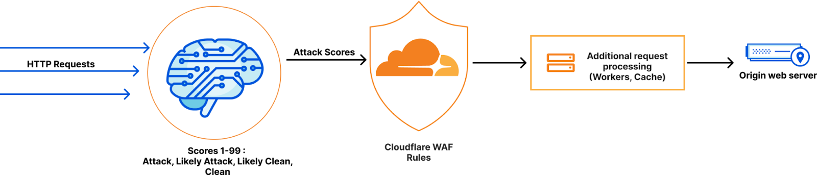
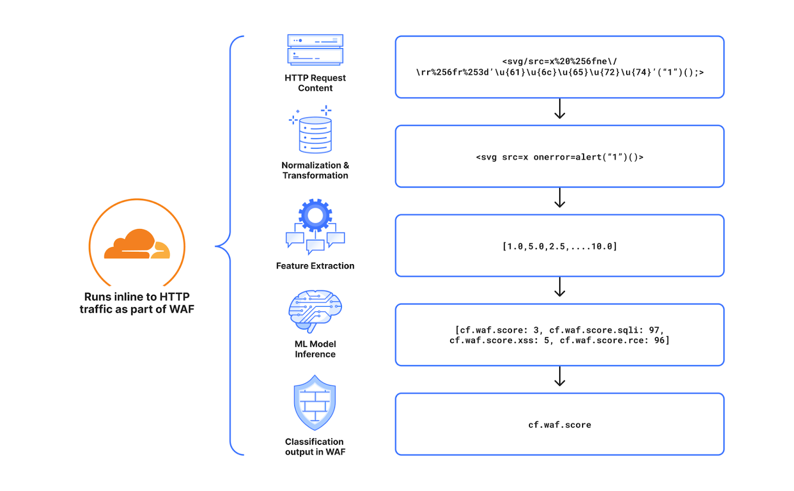
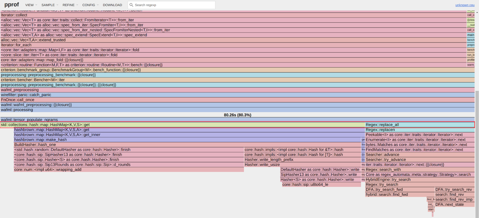


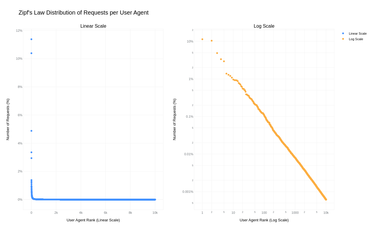
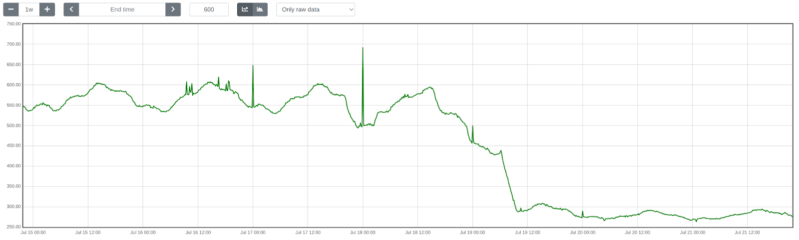


 Salim Tutuncu is a Sr. PSA Specialist on Data & AI, based from Amsterdam with a focus on the EMEA North and EMEA Central regions. With a rich background in the technology sector that spans roles as a Data Engineer, Data Scientist, and Machine Learning Engineer, Salim has built a formidable expertise in navigating the complex landscape of data and artificial intelligence. His current role involves working closely with partners to develop long-term, profitable businesses leveraging the AWS Platform, particularly in Data and AI use cases.
 Angel Conde Manjon is a Sr. PSA Specialist on Data & AI, based in Madrid, and focuses on EMEA South and Israel. He has previously worked on research related to Data Analytics and Artificial Intelligence in diverse European research projects. In his current role, Angel helps partners develop businesses centered on Data and AI.


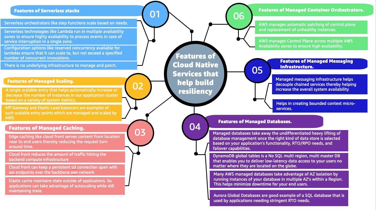


 Chao Pan is a Data Analytics Solutions Architect at Amazon Web Services. He’s responsible for the consultation and design of customers’ big data solution architectures. He has extensive experience in open-source big data. Outside of work, he enjoys hiking.