Post Syndicated from Grab Tech original https://engineering.grab.com/building-hyperlocal-grabmaps
Introduction
Southeast Asia (SEA) is a dynamic market, very different from other parts of the world. When travelling on the road, you may experience fast-changing road restrictions, new roads appearing overnight, and high traffic congestion. To address these challenges, GrabMaps has adapted to the SEA market by leveraging big data solutions. One of the solutions is the integration of hyperlocal data in GrabMaps.
Hyperlocal information is oriented around very small geographical communities and obtained from the local knowledge that our map team gathers. The map team is spread across SEA, enabling us to define clear specifications (e.g. legal speed limits), and validate that our solutions are viable.
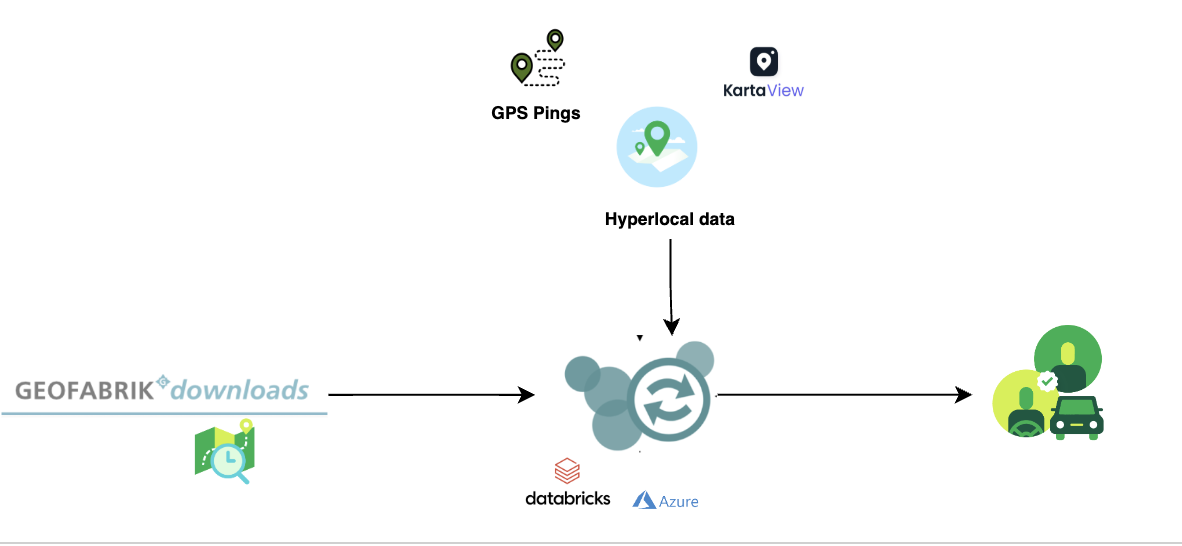
Hyperlocal inputs make our mapping data even more robust, adding to the details collected from our image and probe detection pipelines. Figure 1 shows how data from our detection pipeline is overlaid with hyperlocal data, and then mapped across the SEA region. If you are curious and would like to check out the data yourself, you can download it here.
Processing hyperlocal data
Now let’s go through the process of detecting hyperlocal data.
Download data
GrabMaps is based on OpenStreetMap (OSM). The first step in the process is to download the .pbf file for Asia from geofabrick.de. This .pbf file contains all the data that is available on OSM, such as details of places, trees, and roads. Take for example a park, the .pbf file would contain data on the park name, wheelchair accessibility, and many more.
For this article, we will focus on hyperlocal data related to the road network. For each road, you can obtain data such as the type of road (residential or motorway), direction of traffic (one-way or more), and road name.
Convert data
To take advantage of big data computing, the next step in the process is to convert the .pbf file into Parquet format using a Parquetizer. This will convert the binary data in the .pbf file into a table format. Each road in SEA is now displayed as a row in a table as shown in Figure 2.

Identify hyperlocal data
After the data is prepared, GrabMaps then identifies and inputs all of our hyperlocal data, and delivers a consolidated view to our downstream services. Our hyperlocal data is obtained from various sources, either by looking at geometry, or other attributes in OSM such as the direction of travel and speed limit. We also apply customised rules defined by our local map team, all in a fully automated manner. This enhances the map together with data obtained from our rides and deliveries GPS pings and from KartaView, Grab’s product for imagery collection.
Benefit of our hyperlocal GrabMaps
GrabNav, a turn-by-turn navigation tool available on the Grab driver app, is one of our products that benefits from having hyperlocal data. Here are some hyperlocal data that are made available through our approach:
- Localisation of roads: The country, state/county, or city the road is in
- Language spoken, driving side, and speed limit
- Region-specific default speed regulations
- Consistent name usage using language inference
- Complex attributes like intersection links
To further explain the benefits of this hyperlocal feature, we will use intersection links as an example. In the next section, we will explain how intersection links data is used and how it impacts our driver-partners and passengers.
Identifying hyperlocal data – intersection links
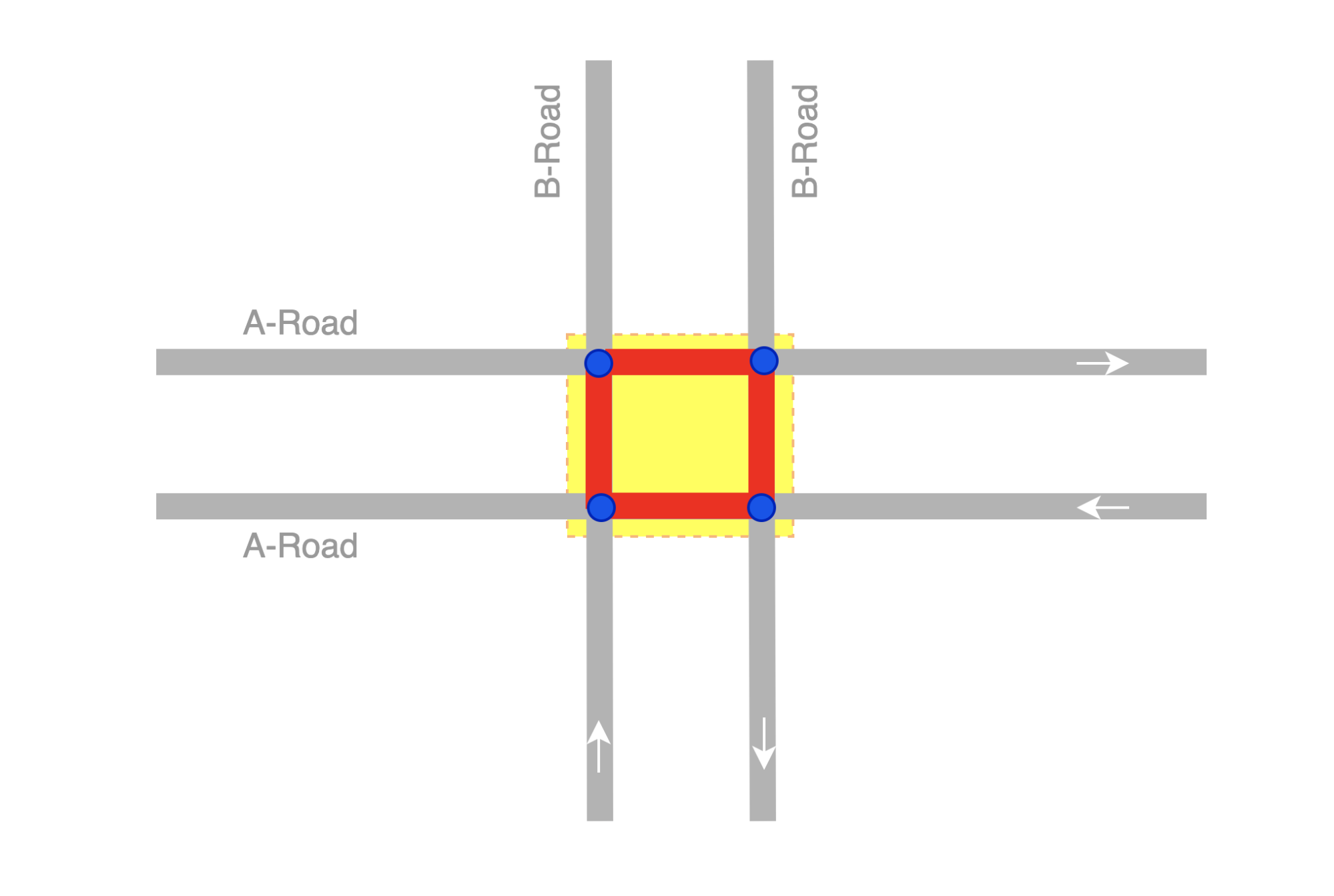
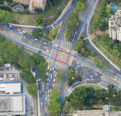
An intersection link is when two or more roads meet. Figure 4 and 5 illustrates what an intersection link looks like in a GrabMaps mock and in OSM.
To locate intersection links in a road network, there are computations involved. We would first combine big data processing (which we do using Spark) with graphs. We use geohash as the unit of processing, and for each geohash, a bi-directional graph is created.
From such resulting graphs, we can determine intersection links if:
- Road segments are parallel
- The roads have the same name
- The roads are one way roads
- Angles and the shape of the road are in the intervals or requirements we seek
Each intersection link we identify is tagged in the map as intersection_links. Our downstream service teams can then identify them by searching for the tag.
Impact
The impact we create with our intersection link can be explained through the following example.
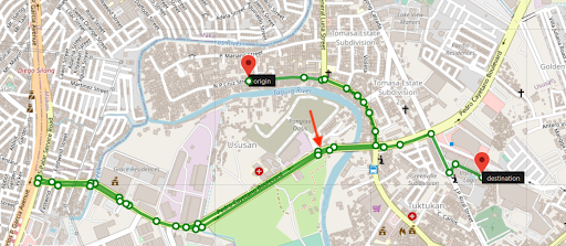
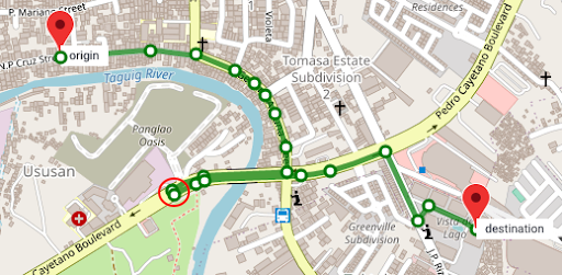
Figure 6 and Figure 7 show two different routes for the same origin and destination. However, you can see that Figure 7 has a shorter route and this is made available by taking an intersection link early on in the route. The highlighted road segment in Figure 7 is an intersection link, tagged by the process we described earlier. The route is now much shorter making GrabNav more efficient in its route suggestion.
There are numerous factors that can impact a driver-partner’s trip, and intersection links are just one example. There are many more features that GrabMaps offers across Grab’s services that allow us to “outserve” our partners.
Conclusion
GrabMaps and GrabNav deliver enriched experiences to our driver-partners. By integrating certain hyperlocal data features, we are also able to provide more accurate pricing for both our driver-partners and passengers. In our mission towards sustainable growth, this is an area that we will keep on improving by leveraging scalable tech solutions.
Join us
Grab is the leading superapp platform in Southeast Asia, providing everyday services that matter to consumers. More than just a ride-hailing and food delivery app, Grab offers a wide range of on-demand services in the region, including mobility, food, package and grocery delivery services, mobile payments, and financial services across 428 cities in eight countries.
Powered by technology and driven by heart, our mission is to drive Southeast Asia forward by creating economic empowerment for everyone. If this mission speaks to you, join our team today!