Tag Archives: Maps

Road localisation in GrabMaps

Post Syndicated from Grab Tech original https://engineering.grab.com/road-localisation-grabmaps

Introduction

In 2022, Grab achieved self-sufficiency in its Geo services. As part of this transition, one crucial step was moving towards using an internally-developed map tailored specifically to the market in which Grab operates. Now that we have full control over the map layer, we can add more data to it or improve it according to the needs of the services running on top. One key aspect that this transition unlocked for us was the possibility of creating hyperlocal data at map level.

For instance, by determining the country to which a road belongs, we can now automatically infer the official language of that country and display the street name in that language. In another example, knowing the country for a specific road, we can automatically infer the driving side (left-handed or right-handed) leading to an improved navigation experience. Furthermore, this capability also enables us to efficiently handle various scenarios. For example, if we know that a road is part of a gated community, an area where our driver partners face restricted access, we can prevent the transit through that area.

These are just some examples of the possibilities from having full control over the map layer. By having an internal map, we can align our maps with specific markets and provide better experiences for our driver-partners and customers.

Background

For all these to be possible, we first needed to localise the roads inside the map. Our goal was to include hyperlocal data into the map, which refers to data that is specific to a certain area, such as a country, city, or even a smaller part of the city like a gated community. At the same time, we aimed to deliver our map with a high cadence, thus, we needed to find the right way to process this large amount of data while continuing to create maps in a cost-effective manner.

Solution

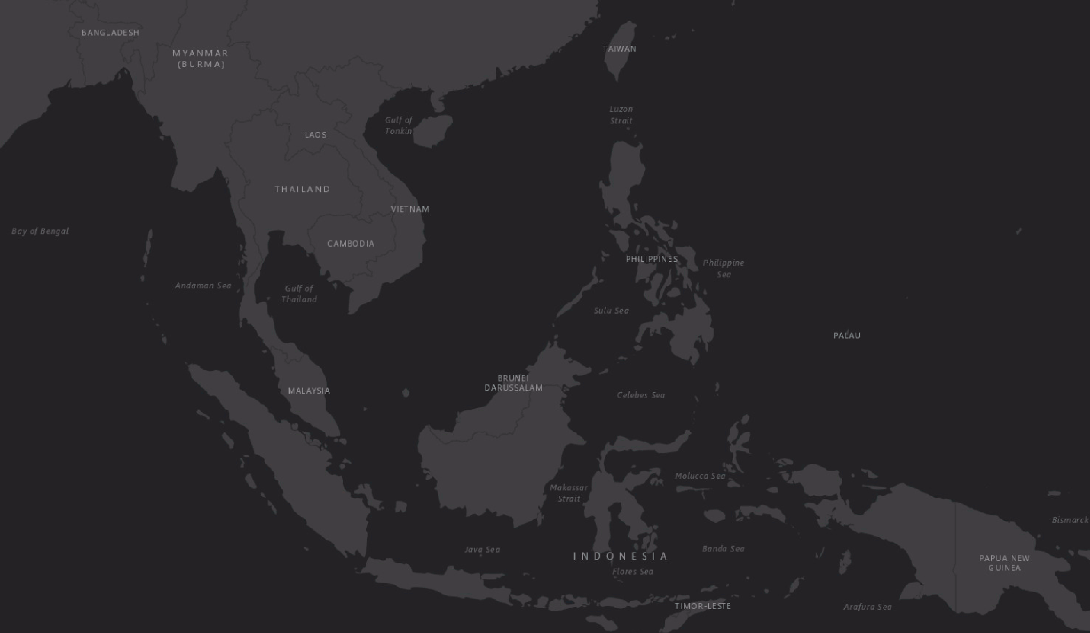
In the following sections of this article, we will use an extract from the Southeast Asia map to provide visual representations of the concepts discussed.

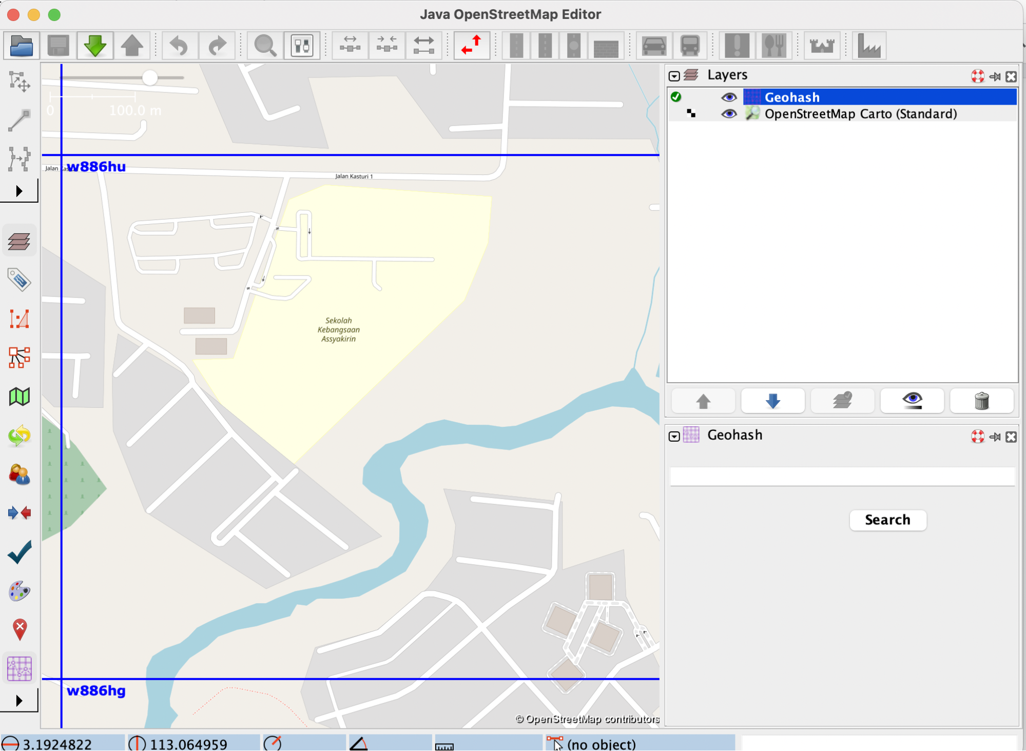
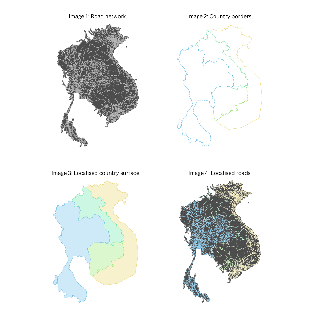
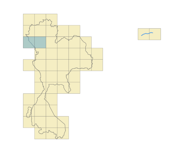
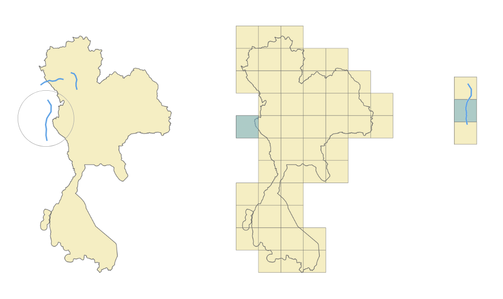
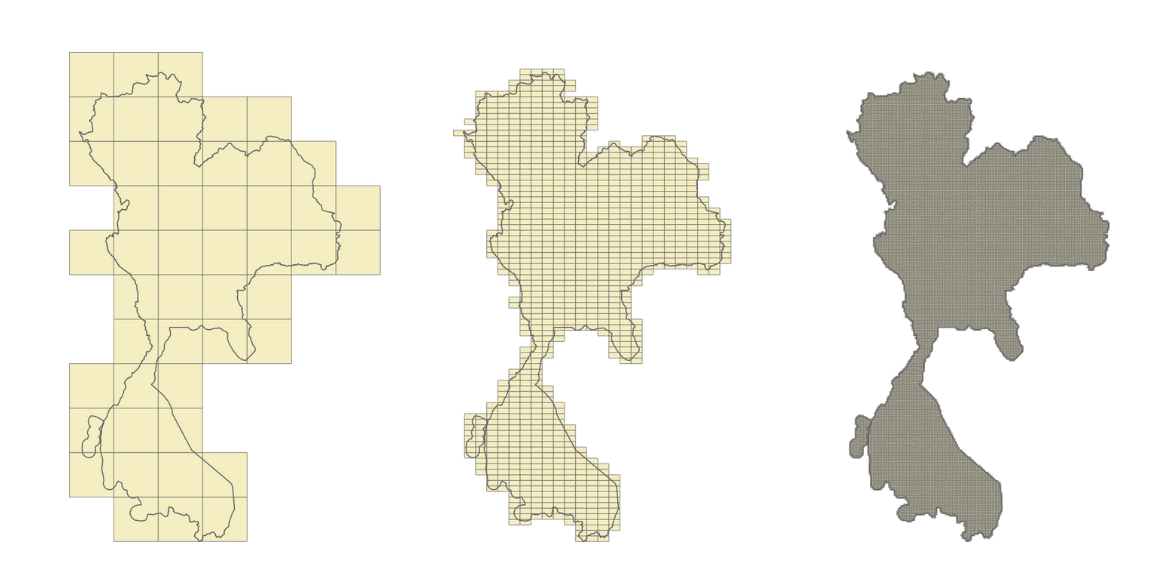
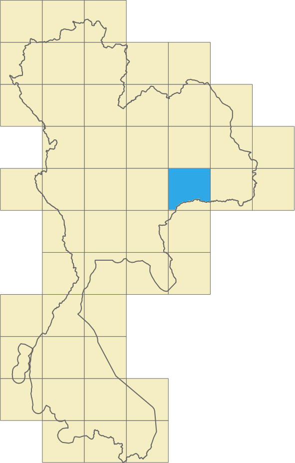
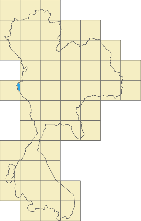
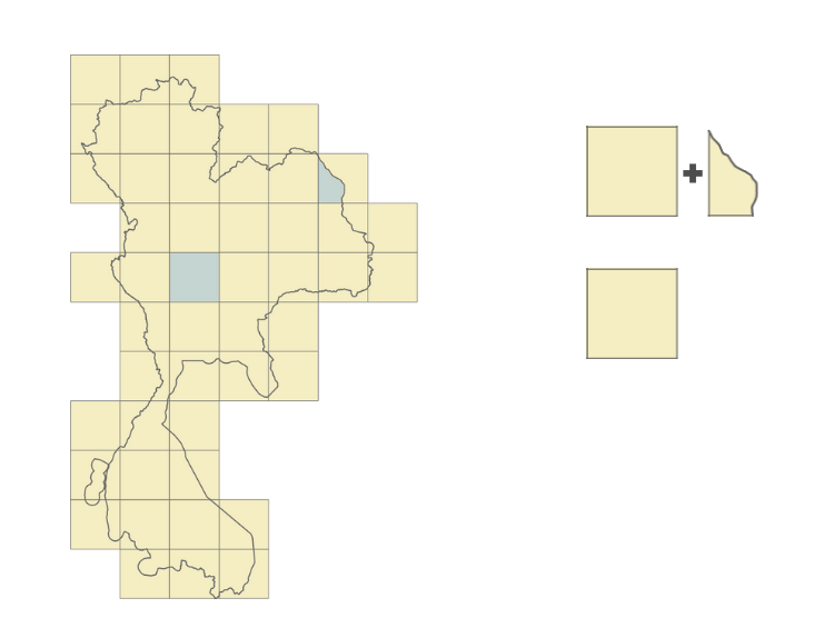
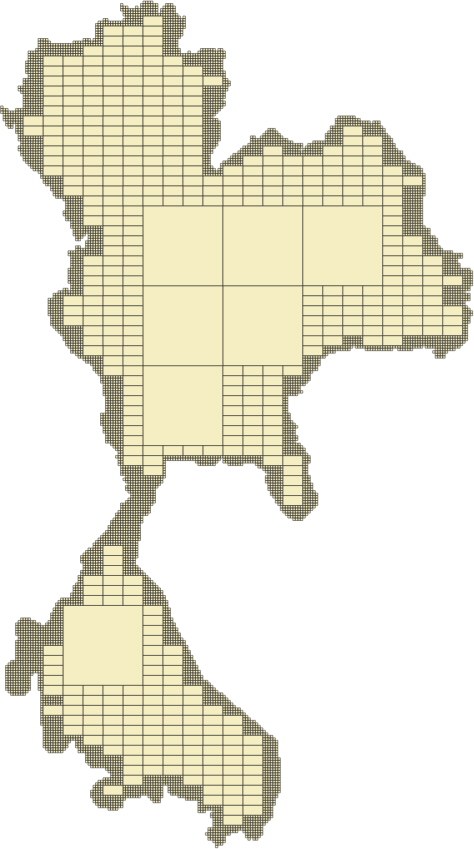
In Figure 1, Image 1 shows a visualisation of the road network, the roads belonging to this area. The coloured lines in Image 2 represent the borders identifying the countries in the same area. Overlapping the information from Image 1 and Image 2, we can extrapolate and say that the entire surface included in a certain border could have the same set of common properties as shown in Image 3. In Image 4, we then proceed with adding localised roads for each area.

Figure 1 – Map of Southeast Asia

For this to be possible, we have to find a way to localise each road and identify its associated country. Once this localisation process is complete, we can replicate all this information specific to a given border onto each individual road. This information includes details such as the country name, driving side, and official language. We can go even further and infer more information, and add hyperlocal data. For example, in Vietnam, we can automatically prevent motorcycle access on the motorways.

Assigning each road on the map to a specific area, such as a country, service area, or subdivision, presents a complex task. So, how can we efficiently accomplish this?

Implementation

The most straightforward approach would be to test the inclusion of each road into each area boundary, but that is easier said than done. With close to 30 million road segments in the Southeast Asia map and over 10 thousand areas, the computational cost of determining inclusion or intersection between a polyline and a polygon is expensive.

Our solution to this challenge involves replacing the expensive yet precise operation with a decent approximation. We introduce a proxy entity, the geohash, and we use it to approximate the areas and also to localise the roads.

We replace the geometrical inclusion with a series of simpler and less expensive operations. First, we conduct an inexpensive precomputation where we identify all the geohases that belong to a certain area or within a defined border. We then identify the geohashes to which the roads belong to. Finally, we use these precomputed values to assign roads to their respective areas. This process is also computationally inexpensive.

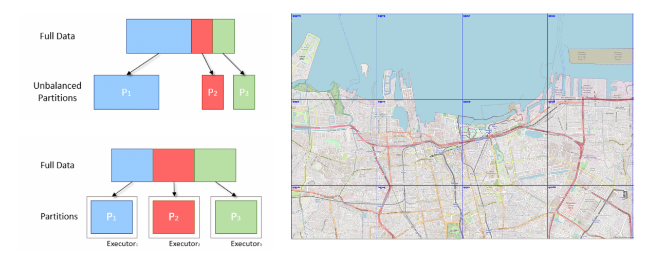
Given the large area we process, we leverage big data techniques to distribute the execution across multiple nodes and thus speed up the operation. We want to deliver the map daily and this is one of the many operations that are part of the map-making process.
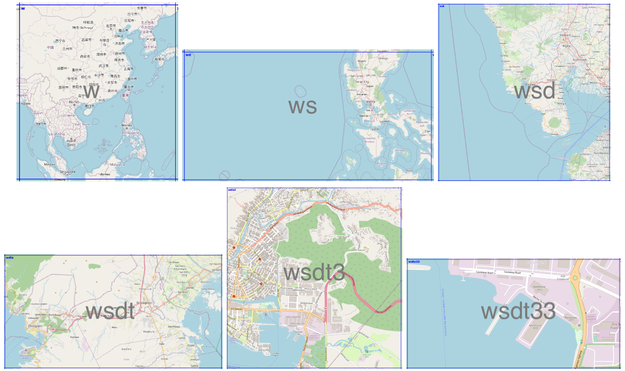
What is a geohash?

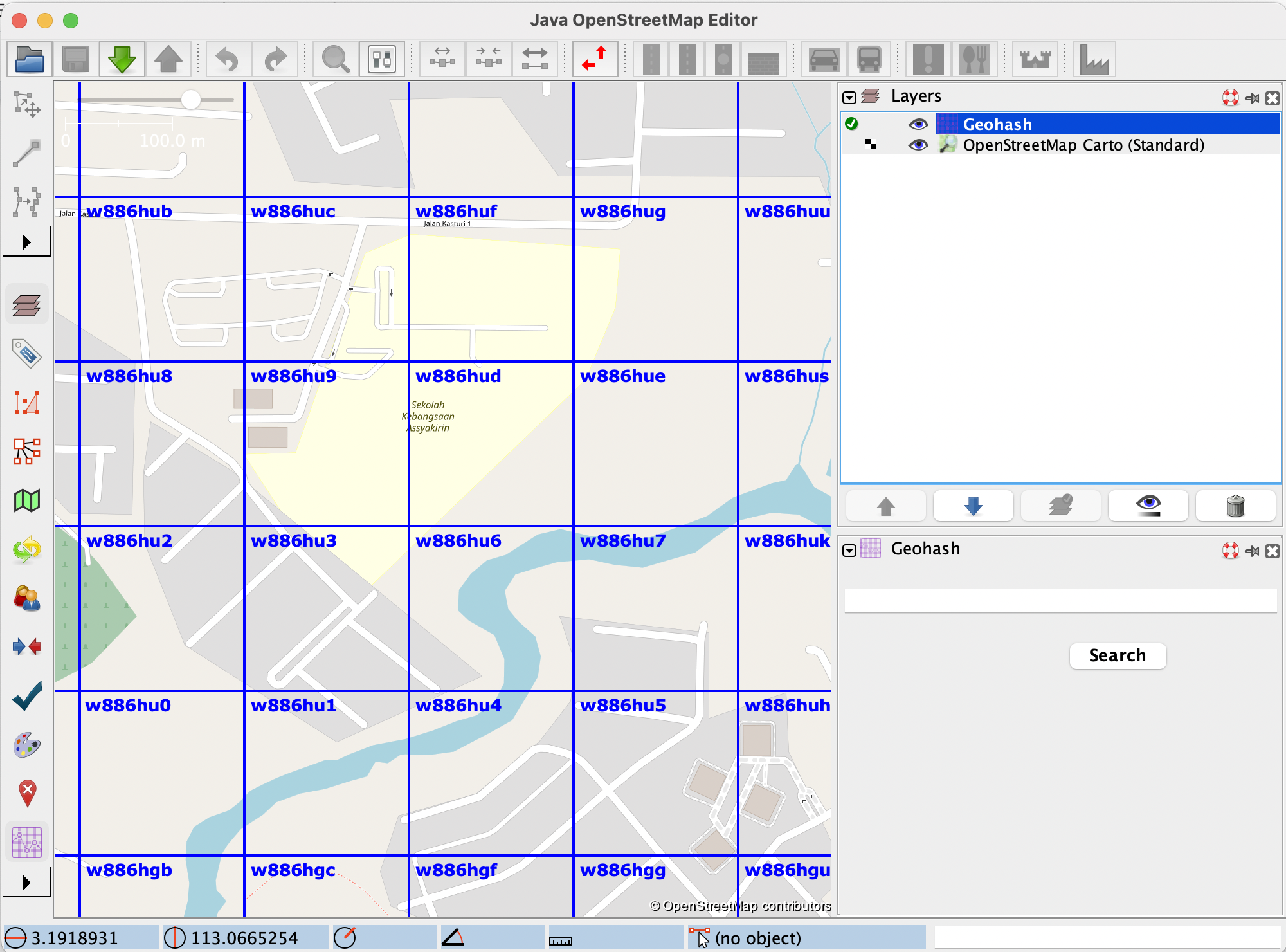
To further understand our implementation we will first explain the geohash concept. A geohash is a unique identifier of a specific region on the Earth. The basic idea is that the Earth is divided into regions of user-defined size and each region is assigned a unique id, which is known as its geohash. For a given location on earth, the geohash algorithm converts its latitude and longitude into a string.

Geohashes uses a Base-32 alphabet encoding system comprising characters ranging from 0 to 9 and A to Z, excluding “A”, “I”, “L” and “O”. Imagine dividing the world into a grid with 32 cells. The first character in a geohash identifies the initial location of one of these 32 cells. Each of these cells are then further subdivided into 32 smaller cells.This subdivision process continues and refines to specific areas in the world. Adding characters to the geohash sub-divides a cell, effectively zooming in to a more detailed area.

The precision factor of the geohash determines the size of the cell. For instance, a precision factor of one creates a cell 5,000 km high and 5,000 km wide. A precision factor of six creates a cell 0.61km high and 1.22 km wide. Furthermore, a precision factor of nine creates a cell 4.77 m high and 4.77 m wide. It is important to note that cells are not always square and can have varying dimensions.

In Figure 2, we have exemplified a geohash 6 grid and its code is wsdt33.

Figure 2 – An example of geohash code wsdt33

Using less expensive operations

Calculating the inclusion of the roads inside a certain border is an expensive operation. However, quantifying the exact expense is challenging as it depends on several factors. One factor is the complexity of the border. Borders are usually irregular and very detailed, as they need to correctly reflect the actual border. The complexity of the road geometry is another factor that plays an important role as roads are not always straight lines.

Figure 3 – Roads to localise

Since this operation is expensive both in terms of cloud cost and time to run, we need to identify a cheaper and faster way that would yield similar results. Knowing that the complexity of the border lines is the cause of the problem, we tried using a different alternative, a rectangle. Calculating the inclusion of a polyline inside a rectangle is a cheaper operation.

Figure 4 – Roads inside a rectangle

So we transformed this large, one step operation, where we test each road segment for inclusion in a border, into a series of smaller operations where we perform the following steps:

  1. Identify all the geohashes that are part of a certain area or belong to a certain border. In this process we include additional areas to make sure that we cover the entire surface inside the border.
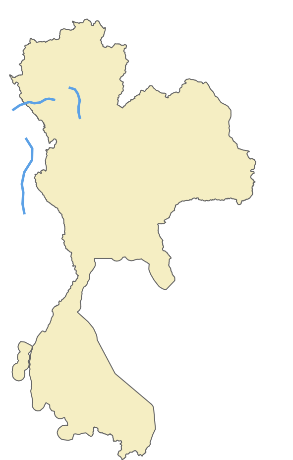
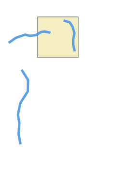
  2. For each road segment, we identify the list of geohashes that it belongs to. A road, depending on its length or depending on its shape, might belong to multiple geohashes.

In Figure 5, we identify that the road belongs to two geohashes and that the two geohashes are part of the border we use.

Figure 5 – Geohashes as proxy

Now, all we need to do is join the two data sets together. This kind of operation is a great candidate for a big data approach, as it allows us to run it in parallel and speed up the processing time.

Precision tradeoff

We mentioned earlier that, for the sake of argument, we replace precision with a decent approximation. Let’s now delve into the real tradeoff by adopting this approach.

The first thing that stands out with this approach is that we traded precision for cost. We are able to reduce the cost as this approach uses less hardware resources and computation time. However, this reduction in precision suffers, particularly for roads located near the borders as they might be wrongly classified.

Going back to the initial example, let’s take the case of the external road, on the left side of the area. As you can see in Figure 6, it is clear that the road does not belong to our border. But when we apply the geohash approach it gets included into the middle geohash.

Figure 6 – Wrong road localisation

Given that just a small part of the geohash falls inside the border, the entire geohash will be classified as belonging to that area, and, as a consequence, the road that belongs to that geohash will be wrongly localised and we’ll end up adding the wrong localisation information to that road. This is clearly a consequence of the precision tradeoff. So, how can we solve this?

Geohash precision

One option is to increase the geohash precision. By using smaller and smaller geohashes, we can better reflect the actual area. As we go deeper and we further split the geohash, we can accurately follow the border. However, a high geohash precision also equates to a computationally intensive operation bringing us back to our initial situation. Therefore, it is crucial to find the right balance between the geohash size and the complexity of operations.

Figure 7 – Geohash precision

Geohash coverage percentage

To find a balance between precision and data loss, we looked into calculating the geohash coverage percentage. For example, in Figure 8, the blue geohash is entirely within the border. Here we can say that it has a 100% geohash coverage.

Figure 8 – Geohash inside the border

However, take for example the geohash in Figure 9. It touches the border and has only around 80% of its surface inside the area. Given that most of its surface is within the border, we still can say that it belongs to the area.

Figure 9 – Geohash partially inside the border

Let’s look at another example. In Figure 10, only a small part of the geohash is within the border. We can say that the geohash coverage percentage here is around 5%. For these cases, it becomes difficult for us to determine whether the geohash does belong to the area. What would be a good tradeoff in this case?

Figure 10 – Geohash barely inside the border

Border shape

To go one step further, we can consider a mixed solution, where we use the border shape but only for the geohashes touching the border. This would still be an intensive computational operation but the number of roads located in these geohashes will be much smaller, so it is still a gain.

For the geohashes with full coverage inside the area, we’ll use the geohash for the localisation, the simpler operation. For the geohashes that are near the border, we’ll use a different approach. To increase the precision around the borders, we can cut the geohash following the border’s shape. Instead of having a rectangle, we’ll use a more complex shape which is still simpler than the initial border shape.

Figure 11 – Geohash following a border’s shape

Result

We began with a simple approach and we enhanced it to improve precision. This also increased the complexity of the operation. We then asked, what are the actual gains? Was it worthwhile to go through all this process? In this section, we put this to the test.

We first created a benchmark by taking a small sample of the data and ran the localisation process on a laptop. The sample comprised approximately 2% of the borders and 0.0014% of the roads. We ran the localisation process using two approaches.

  • With the first approach, we calculated the intersection between all the roads and borders. The entire operation took around 38 minutes.
  • For the second approach, we optimised the operation using geohashes. In this approach, the runtime was only 78 seconds (1.3 minutes).

However, it is important to note that this is not an apples-to-apples comparison. The operation that we measured was the localisation of the roads but we did not include the border filling operation where we fill the borders with geohashes. This is because this operation does not need to be run every time. It can be run once and reused multiple times.

Though not often required, it is still crucial to understand and consider the operation of precomputing areas and filling borders with geohashes. The precomputation process depends on several factors:

  • Number and shape of the borders – The more borders and the more complex the borders are, the longer the operation will take.
  • Geohash precision – How accurate do we need our localisation to be? The more accurate it needs to be, the longer it will take.
  • Hardware availability

Going back to our hypothesis, although this precomputation might be expensive, it is rarely run as the borders don’t change often and can be triggered only when needed. However, regular computation, where we find the area to which each road belongs to, is often run as the roads change constantly. In our system, we run this localisation for each map processing.

We can also further optimise this process by applying the opposite approach. Geohashes that have full coverage inside a border can be merged together into larger geohashes thus simplifying the computation inside the border. In the end, we can have a solution that is fully optimised for our needs with the best cost-to-performance ratio.

Figure 12 – Optimised geohashes

Conclusion

Although geohashes seem to be the right solution for this kind of problem, we also need to monitor their content. One consideration is the road density inside a geohash. For example, a geohash inside a city centre usually has a lot of roads while one in the countryside may have much less. We need to consider this aspect to have a balanced computation operation and take full advantage of the big data approach. In our case, we achieve this balance by considering the number of road kilometres within a geohash.

Figure 13 – Unbalanced data

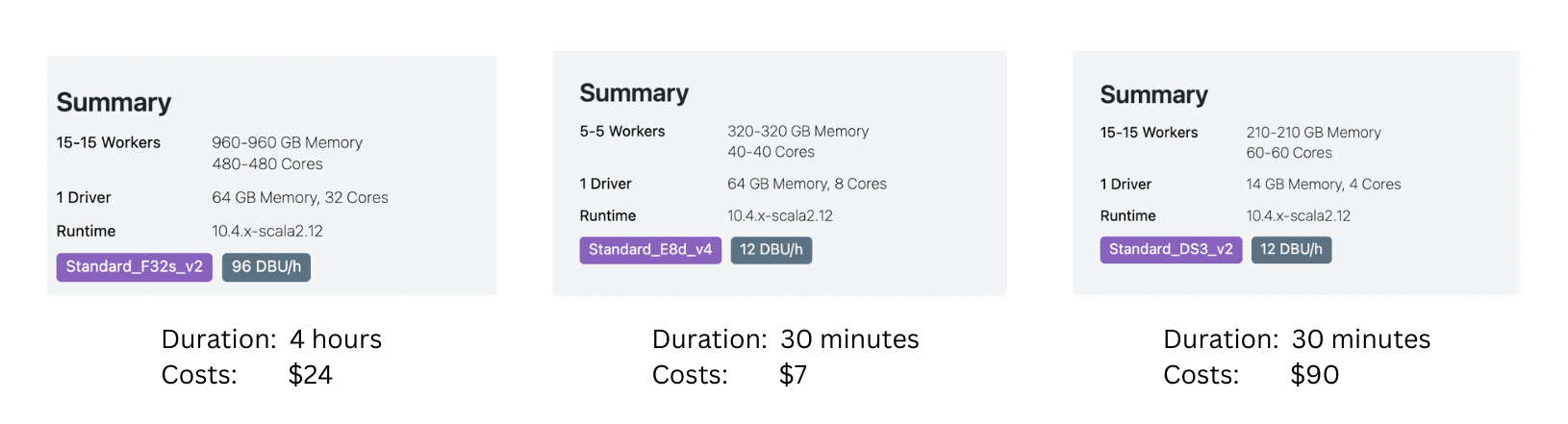
Additionally, the resources that we choose also matter. To optimise time and cost, we need to find the right balance between the running time and resource cost. As shown in Figure 14, based on a sample data we ran, sometimes, we get the best result when using smaller machines.

Figure 14 – Cost vs runtime

The achievements and insights showcased in this article are indebted to the contributions made by Mihai Chintoanu. His expertise and collaborative efforts have profoundly enriched the content and findings presented herein.

Join us

Grab is the leading superapp platform in Southeast Asia, providing everyday services that matter to consumers. More than just a ride-hailing and food delivery app, Grab offers a wide range of on-demand services in the region, including mobility, food, package and grocery delivery services, mobile payments, and financial services across 428 cities in eight countries.

Powered by technology and driven by heart, our mission is to drive Southeast Asia forward by creating economic empowerment for everyone. If this mission speaks to you, join our team today!

Building hyperlocal GrabMaps

Post Syndicated from Grab Tech original https://engineering.grab.com/building-hyperlocal-grabmaps

Introduction

Southeast Asia (SEA) is a dynamic market, very different from other parts of the world. When travelling on the road, you may experience fast-changing road restrictions, new roads appearing overnight, and high traffic congestion. To address these challenges, GrabMaps has adapted to the SEA market by leveraging big data solutions. One of the solutions is the integration of hyperlocal data in GrabMaps.

Hyperlocal information is oriented around very small geographical communities and obtained from the local knowledge that our map team gathers. The map team is spread across SEA, enabling us to define clear specifications (e.g. legal speed limits), and validate that our solutions are viable.

Figure 1 – Map showing detections from images and probe data, and hyperlocal data.

Hyperlocal inputs make our mapping data even more robust, adding to the details collected from our image and probe detection pipelines. Figure 1 shows how data from our detection pipeline is overlaid with hyperlocal data, and then mapped across the SEA region. If you are curious and would like to check out the data yourself, you can download it here.

Processing hyperlocal data

Now let’s go through the process of detecting hyperlocal data.

Download data

GrabMaps is based on OpenStreetMap (OSM). The first step in the process is to download the .pbf file for Asia from geofabrick.de. This .pbf file contains all the data that is available on OSM, such as details of places, trees, and roads. Take for example a park, the .pbf file would contain data on the park name, wheelchair accessibility, and many more.

For this article, we will focus on hyperlocal data related to the road network. For each road, you can obtain data such as the type of road (residential or motorway), direction of traffic (one-way or more), and road name.

Convert data

To take advantage of big data computing, the next step in the process is to convert the .pbf file into Parquet format using a Parquetizer. This will convert the binary data in the .pbf file into a table format. Each road in SEA is now displayed as a row in a table as shown in Figure 2.

Figure 2 – Road data in Parquet format.

Identify hyperlocal data

After the data is prepared, GrabMaps then identifies and inputs all of our hyperlocal data, and delivers a consolidated view to our downstream services. Our hyperlocal data is obtained from various sources, either by looking at geometry, or other attributes in OSM such as the direction of travel and speed limit. We also apply customised rules defined by our local map team, all in a fully automated manner. This enhances the map together with data obtained from our rides and deliveries GPS pings and from KartaView, Grab’s product for imagery collection.

Figure 3 – Architecture diagram showing how hyperlocal data is integrated into GrabMaps.

Benefit of our hyperlocal GrabMaps

GrabNav, a turn-by-turn navigation tool available on the Grab driver app, is one of our products that benefits from having hyperlocal data. Here are some hyperlocal data that are made available through our approach:

  • Localisation of roads: The country, state/county, or city the road is in
  • Language spoken, driving side, and speed limit
  • Region-specific default speed regulations
  • Consistent name usage using language inference
  • Complex attributes like intersection links

To further explain the benefits of this hyperlocal feature, we will use intersection links as an example. In the next section, we will explain how intersection links data is used and how it impacts our driver-partners and passengers.

An intersection link is when two or more roads meet. Figure 4 and 5 illustrates what an intersection link looks like in a GrabMaps mock and in OSM.

Figure 4 – Mock of an intersection link.
Figure 5 – Intersection link illustration from a real road network in OSM.

To locate intersection links in a road network, there are computations involved. We would first combine big data processing (which we do using Spark) with graphs. We use geohash as the unit of processing, and for each geohash, a bi-directional graph is created.

From such resulting graphs, we can determine intersection links if:

  • Road segments are parallel
  • The roads have the same name
  • The roads are one way roads
  • Angles and the shape of the road are in the intervals or requirements we seek

Each intersection link we identify is tagged in the map as intersection_links. Our downstream service teams can then identify them by searching for the tag.

Impact

The impact we create with our intersection link can be explained through the following example.

Figure 6 – Longer route, without GrabMaps intersection link feature. The arrow indicates where the route should have suggested a U-turn.
Figure 7 – Shorter route using GrabMaps by taking a closer link between two main roads.

Figure 6 and Figure 7 show two different routes for the same origin and destination. However, you can see that Figure 7 has a shorter route and this is made available by taking an intersection link early on in the route. The highlighted road segment in Figure 7 is an intersection link, tagged by the process we described earlier. The route is now much shorter making GrabNav more efficient in its route suggestion.

There are numerous factors that can impact a driver-partner’s trip, and intersection links are just one example. There are many more features that GrabMaps offers across Grab’s services that allow us to “outserve” our partners.

Conclusion

GrabMaps and GrabNav deliver enriched experiences to our driver-partners. By integrating certain hyperlocal data features, we are also able to provide more accurate pricing for both our driver-partners and passengers. In our mission towards sustainable growth, this is an area that we will keep on improving by leveraging scalable tech solutions.

Join us

Grab is the leading superapp platform in Southeast Asia, providing everyday services that matter to consumers. More than just a ride-hailing and food delivery app, Grab offers a wide range of on-demand services in the region, including mobility, food, package and grocery delivery services, mobile payments, and financial services across 428 cities in eight countries.

Powered by technology and driven by heart, our mission is to drive Southeast Asia forward by creating economic empowerment for everyone. If this mission speaks to you, join our team today!

New zoom freezing feature for Geohash plugin

Post Syndicated from Grab Tech original https://engineering.grab.com/geohash-plugin

Introduction

Geohash is an encoding system with a unique identifier for each region on the planet. Therefore, all geohash units can be associated with an individual set of digits and letters.

Geohash is a plugin built by Grab that is available in the Java OpenStreetMap Editor (JOSM) tool, which comes in handy for those who work on precise areas based on geohash units.

Background

Up until recently, users of the Geohash JOSM plugin were unable to stop the displaying of new geohashes with every zoom-in or zoom-out. This meant that every time they changed the zoom, new geohashes would be displayed, and this became bothersome for many users when it was unneeded. The previous behaviour of the plugin when zooming in and out is depicted in the following short video:


This led to the implementation of the zoom freeze feature, which helps users toggle between Enable zoom freeze and Disable zoom freeze, based on their needs.

Solution

As you can see in the following image, a new label was created with the purpose of freezing or unfreezing the display of new geohashes with each zoom change:


By default, this label says “Enable zoom freeze”, and when zoom freezing is enabled, the label changes to “Disable zoom freeze”.

In order to see how zoom freezing works, let’s consider the following example: a user wants to zoom inside the geohash with the code w886hu, without triggering the display of smaller geohashes inside of it. For this purpose, the user will enable the zoom freezing feature by clicking on the label, and then they will proceed with the zoom. The map will look like this:


It is apparent from the image that no new geohashes were created. Now, let’s say the user has finished what they wanted to do, and wants to go back to the “normal” geohash visualisation mode, which means disabling the zoom freeze option. After clicking on the label that now says ‘Disable zoom freeze’, new, smaller geohashes will be displayed, according to the current zoom level:


The functionality is illustrated in the following short video:


Another effect that enabling zoom freeze has is that it disables the ‘Display larger geohashes’ and ‘Display smaller geohashes’ options, since the geohashes are now fixed. The following images show how these options work before and after disabling zoom freeze:


To conclude, we believe that the release of this new feature will benefit users by making it more comfortable for them to zoom in and out of a map. By turning off the display of new geohashes when this is unwanted, map readability is improved, and this translates to a better user experience.

Impact/Limitations

In order to start using this new feature, users need to update the Geohash JOSM plugin.

What’s next?

Grab has come a long way in map-making, from using open source map-making software and developing its own suite of map-making tools to contributing to the open-source map community and building and launching GrabMaps. To find out more, read How KartaCam powers GrabMaps and KartaCam delivers comprehensive, cost-effective mapping data.

Join us

Grab is the leading superapp platform in Southeast Asia, providing everyday services that matter to consumers. More than just a ride-hailing and food delivery app, Grab offers a wide range of on-demand services in the region, including mobility, food, package and grocery delivery services, mobile payments, and financial services across 428 cities in eight countries.

Powered by technology and driven by heart, our mission is to drive Southeast Asia forward by creating economic empowerment for everyone. If this mission speaks to you, join our team today!

How KartaCam powers GrabMaps

Post Syndicated from Grab Tech original https://engineering.grab.com/kartacam-powers-grabmaps

Introduction

The foundation for making any map is in imagery, but due to the complexity and dynamism of the real world, it is difficult for companies to collect high-quality, fresh images in an efficient yet low-cost manner. This is the case for Grab’s Geo team as well.

Traditional map-making methods rely on professional-grade cameras that provide high resolution images to collect mapping imagery. These images are rich in content and detail, providing a good snapshot of the real world. However, we see two major challenges with this approach.

The first is high cost. Professional cameras are too expensive to use at scale, especially in an emerging region like Southeast Asia. Apart from high equipment cost, operational cost is also high as local operation teams need professional training before collecting imagery.

The other major challenge, related to the first, is that imagery will not be refreshed in a timely manner because of the high cost and operational effort required. It typically takes months or years before imagery is refreshed, which means maps get outdated easily.

Compared to traditional collection methods, there are more affordable alternatives that some emerging map providers are using, such as crowdsourced collection done with smartphones or other consumer-grade action cameras. This allows more timely imagery refresh at a much lower cost.

That said, there are several challenges with crowdsourcing imagery, such as:

  • Inconsistent quality in collected images.
  • Low operational efficiency as cameras and smartphones are not optimised for mapping.
  • Unreliable location accuracy.

In order to solve the challenges above, we started building our own artificial intelligence (AI) camera called KartaCam.

What is KartaCam?

Designed specifically for map-making, KartaCam is a lightweight camera that is easy to operate. It is everything you need for accurate and efficient image collection. KartaCam is powered by edge AI, and mainly comprises a camera module, a dual-band Global Navigation Satellite System (GNSS) module, and a built-in 4G Long-Term Evolution (LTE) module.

KartaCam

Camera module

The camera module or optical design of KartaCam focuses on several key features:

  • Wide field of vision (FOV): A wide FOV to capture as many scenes and details as possible without requiring additional trips. A single KartaCam has a wide lens FOV of >150° and when we use four KartaCams together, each facing a different direction, we increase the FOV to 360°.
  • High image quality: A combination of high-definition optical lens and a high-resolution pixel image sensor can help to achieve better image quality. KartaCam uses a high-quality 12MP image sensor.
  • Ease of use: Portable and easy to start using for people with little to no photography training. At Grab, we can easily deploy KartaCam to our fleet of driver-partners to map our region as they regularly travel these roads while ferrying passengers or making deliveries.

Edge AI for smart capturing on edge

Each KartaCam device is also equipped with edge AI, which enables AI computations to operate closer to the actual data – in our case, imagery collection. With edge AI, we can make decisions about imagery collection (i.e. upload, delete or recapture) at the device-level.

To help with these decisions, we use a series of edge AI models and algorithms that are executed immediately after each image capture such as:

  • Scene recognition model: For efficient map-making, we ensure that we make the right screen verdicts, meaning we only upload and process the right scene images. Unqualified images such as indoor, raining, and cloudy images are deleted directly on the KartaCam device. Joint detection algorithms are deployed in some instances to improve the accuracy of scene verdicts. For example, to detect indoor recording we look at a combination of driver moving speed, Inertial Measurement Units (IMU) data and edge AI image detection.

  • Image quality (IQ) checking AI model: The quality of the images collected is paramount for map-making. Only qualified images judged by our IQ classification algorithm will be uploaded while those that are blurry or considered low-quality will be deleted. Once an unqualified image is detected (usually within the next second), a new image is captured, improving the success rate of collection.

  • Object detection AI model: Only roadside images that contain relevant map-making content such as traffic signs, lights, and Point of Interest (POI) text are uploaded.

  • Privacy information detection: Edge AI also helps protect privacy when collecting street images for map-making. It automatically blurs private information such as pedestrians’ faces and car plate numbers before uploading, ensuring adequate privacy protection.


Better positioning with a dual-band GNSS module

The Global Positioning System (GPS) mainly uses two frequency bands: L1 and L5. Most traditional phone or GPS modules only support the legacy GPS L1 band, while modern GPS modules support both L1 and L5. KartaCam leverages the L5 band which provides improved signal structure, transmission capabilities, and a wider bandwidth that can reduce multipath error, interference, and noise impacts. In addition, KartaCam uses a fine-tuned high-quality ceramic antenna that, together with the dual frequency band GPS module, greatly improves positioning accuracy.

Keeping KartaCam connected

KartaCam has a built-in 4G LTE module that ensures it is always connected and can be remotely managed. The KartaCam management portal can monitor camera settings like resolution and capturing intervals, even in edge AI machine learning models. This makes it easy for Grab’s map ops team and drivers to configure their cameras and upload captured images in a timely manner.

Enhancing KartaCam

KartaCam 360: Capturing a panorama view

To improve single collection trip efficiency, we group four KartaCams together to collect 360° images. The four cameras can be synchronised within milliseconds and the collected images are stitched together in a panoramic view.

With KartaCam 360, we can increase the number of images collected in a single trip. According to Grab’s benchmark testing in Singapore and Jakarta, the POI information collected by KartaCam 360 is comparable to that of professional cameras, which cost about 20x more.

KartaCam 360 & Scooter mount
Image sample from KartaCam 360

KartaCam and the image collection workflow

KartaCam, together with other GrabMaps imagery tools, provides a highly efficient, end-to-end, low-cost, and edge AI-powered smart solution to map the region. KartaCam is fully integrated as part of our map-making workflow.

Our map-making solution includes the following components:

  • Collection management tool – Platform that defines map collection tasks for our driver-partners.
  • KartaView application – Mobile application provides map collection tasks and handles crowdsourced imagery collection.
  • KartaCam – Camera device connected to KartaView via Bluetooth and equipped with edge automatic processing for imagery capturing according to the task accepted.
  • Camera management tool – Handles camera parameters and settings for all KartaCam devices and can remotely control the KartaCam.
  • Automatic processing – Collected images are processed for quality check, stitching, and personal identification information (PII) blurring.
  • KartaView imagery platform – Processed images are then uploaded and the driver-partner receives payment.

In a future article, we will dive deeper into the technology behind KartaView and its role in GrabMaps.

Impact

At the moment, Grab is rolling out thousands of KartaCams to all locations across Southeast Asia where Grab operates. This saves operational costs while improving the efficiency and quality of our data collection.


Better data quality and more map attributes

Due to the excellent image quality, wide FOV coverage, accurate GPS positioning, and sensor data, the 360° images captured by KartaCam 360 also register detailed map attributes like POIs, traffic signs, and address plates. This will help us build a high quality map with rich and accurate content.


Reducing operational costs

Based on our research, the hardware cost for KartaCam 360 is significantly lower compared to similar professional cameras in the market. This makes it a more feasible option to scale up in Southeast Asia as the preferred tool for crowdsourcing imagery collection.

With image quality checks and detection conducted at the edge, we can avoid re-collections and also ensure that only qualified images are uploaded. These result in saving time as well as operational and upload costs.

Upholding privacy standards

KartaCam automatically blurs captured images that contain PII, like faces and licence plates directly from the edge devices. This means that all sensitive information is removed at this stage and is never uploaded to Grab servers.

On-the-edge blurring example

What’s next?

Moving forward, Grab will continue to enhance KartaCam’s performance in the following aspects:

  • Further improve image quality with better image sensors, unique optical components, and state-of-art Image Signal Processor (ISP).
  • Make KartaCam compatible with Light Detection And Ranging (LIDAR) for high-definition collection and indoor use cases.
  • Improve GNSS module performance with higher sampling frequency and accuracy, and integrate new technology like Real-Time Kinematic (RTK) and Precise Point Positioning (PPP) solutions to further improve the positioning accuracy. When combined with sensor fusion from IMU sensors, we can improve positioning accuracy for map-making further.
  • Improve usability, integration, and enhance imagery collection and portability for KartaCam so driver-partners can easily capture mapping data. 
  • Explore new product concepts for future passive street imagery collection.

To find out more about how KartaCam delivers comprehensive cost-effective mapping data, check out this article.

Join us

Grab is the leading superapp platform in Southeast Asia, providing everyday services that matter to consumers. More than just a ride-hailing and food delivery app, Grab offers a wide range of on-demand services in the region, including mobility, food, package and grocery delivery services, mobile payments, and financial services across 428 cities in eight countries.

Powered by technology and driven by heart, our mission is to drive Southeast Asia forward by creating economic empowerment for everyone. If this mission speaks to you, join our team today!

References

What’s new in Zabbix 6.0 LTS by Artūrs Lontons / Zabbix Summit Online 2021

Post Syndicated from Arturs Lontons original https://blog.zabbix.com/whats-new-in-zabbix-6-0-lts-by-arturs-lontons-zabbix-summit-online-2021/17761/

Zabbix 6.0 LTS comes packed with many new enterprise-level features and improvements. Join Artūrs Lontons and take a look at some of the major features that will be available with the release of Zabbix 6.0 LTS.

The full recording of the speech is available on the official Zabbix Youtube channel.

If we look at the Zabbix roadmap and Zabbix 6.0 LTS release in particular, we can see that one of the main focuses of Zabbix development is releasing features that solve many complex enterprise-grade problems and use cases. Zabbix 6.0 LTS aims to:

  • Solve enterprise-level security and redundancy requirements
  • Improve performance for large Zabbix instances
  • Provide additional value to different types of Zabbix users – DevOPS and ITOps teams, Business process owner, Managers
  • Continue to extend Zabbix monitoring and data collection capabilities
  • Provide continued delivery of official integrations with 3rd party systems

Let’s take a look at the specific Zabbix 6.0 LTS features that can guide us towards achieving these goals.

Zabbix server High Availability cluster

With the release of Zabbix 6.0 LTS, Zabbix administrators will now have the ability to deploy Zabbix server HA cluster out-of-the-box. No additional tools are required to achieve this.

Zabbix server HA cluster supports an unlimited number of Zabbix server nodes. All nodes will use the same database backend – this is where the status of all nodes will be stored in the ha_node table. Nodes will report their status every 5 seconds by updating the corresponding record in the ha_node table.

To enable High availability, you will first have to define a new parameter in the Zabbix server configuration file: HANodeName

  • Empty by default
  • This parameter should contain an arbitrary name of the HA node
  • Providing value to this parameter will enable Zabbix server cluster mode

Standby nodes monitor the last access time of the active node from the ha_node table.

  • If the difference between last access time and current time reaches the failover delay, the cluster fails over to the standby node
  • Failover operation is logged in the Zabbix server log

It is possible to define a custom failover delay – a time window after which an unreachable active node is considered lost and failover to one of the standby nodes takes place.

As for the Zabbix proxies, the Server parameter in the Zabbix proxy configuration file now supports multiple addresses separated by a semicolon. The proxy will attempt to connect to each of the nodes until it succeeds.

Other HA cluster related features:

  • New command-line options to check HA cluster status
  • hanode.get API method to obtain the list of HA nodes
  • The new internal check provides LLD information to discover Zabbix server HA nodes
  • HA Failover event logged in the Zabbix Audit log
  • Zabbix Frontend will automatically switch to the active Zabbix server node

You can find a more detailed look at the Zabbix Server HA cluster feature in the Zabbix Summit Online 2021 speech dedicated to the topic.

Business service monitoring

The Services section has received a complete redesign in Zabbix 6.0 LTS. Business Service Monitoring (BSM) enables Zabbix administrators to define services of varying complexity and monitor their status.

BSM provides added value in a multitude of use cases, where we wish to define and monitor services based on:

  • Server clusters
  • Services that utilize load balancing
  • Services that consist of a complex IT stack
  • Systems with redundant components in place
  • And more

Business Service monitoring has been designed with scalability in mind. Zabbix is capable of monitoring over 100k services on a single Zabbix instance.

For our Business Service example, we used a website, which depends on multiple components such as the network connection, DB backend, Application server, and more. We can see that the service status calculation is done by utilizing tags and deciding if the existing problems will affect the service based on the problem tags.

In Zabbix 6.0 LTS there are many ways how service status calculations can be performed. In case of a problem, the service state can be changed to:

  • The most critical problem severity, based on the child service problem severities
  • The most critical problem severity, based on the child service problem severities, only if all child services are in a problem state
  • The service is set to constantly be in an OK state

Changing the service status to a specific problem severity if:

  • At least N or N% of child services have a specific status
  • Define service weights and calculate the service status based on the service weights

There are many other additional features, all of which are covered in our Zabbix Summit Online 2021 speech dedicated to Business Service monitoring:

  • Ability to define permissions on specific services
  • SLA monitoring
  • Business Service root cause analysis
  • Receive alerts and react on Business Service status change
  • Define Business Service permissions for multi-tenant environments

New Audit log schema

The existing audit log has been redesigned from scratch and now supports detailed logging for both Zabbix server and Zabbix frontend operations:

  • Zabbix 6.0 LTS introduces a new database structure for the Audit log
  • Collision resistant IDs (CUID) will be used for ID generation to prevent audit log row locks
  • Audit log records will be added in bulk SQL requests
  • Introducing Recordset ID column. This will help users recognize which changes have been made in a particular operation

The goal of the Zabbix 6.0 LTS audit log redesign is to provide reliable and detailed audit logging while minimizing the potential performance impact on large Zabbix instances:

  • Detailed logging of both Zabbix frontend and Zabbix server records
  • Designed with minimal performance impact in mind
  • Accessible via Zabbix API

Implementing the new audit log schema is an ongoing effort – further improvements will be done throughout the Zabbix update life cycle.

Machine learning

New trend functions have been added which utilize machine learning to perform anomaly detection and baseline monitoring:

  • New trend function – trendstl, allows you to detect anomalous metric behavior
  • New trend function – baselinewma, returns baseline by averaging data periods in seasons
  • New trend function – baselinedev, returns the number of standard deviations

An in-depth look into Machine learning in Zabbix 6.0 LTS is covered in our Zabbix Summit Online 2021 speech dedicated to machine learning, anomaly detection, and baseline monitoring.

New ways to visualize your data

Collecting and processing metrics is just a part of the monitoring equation. Visualization and the ability to display our infrastructure status in a single pane of glass are also vital to large environments. Zabbix 6.0 LTS adds multiple new visualization options while also improving the existing features.

  • The data table widget allows you to create a summary view for the related metric status on your hosts
  • The Top N and Bottom N functions of the data table widget allow you to have an overview of your highest or lowest item values
  • The single item widget allows you to display values for a single metric
  • Improvements to the existing vector graphs such as the ability to reference individual items and more
  • The SLA report widget displays the current SLA for services filtered by service tags

We are proud to announce that Zabbix 6.0 LTS will provide a native Geomap widget. Now you can take a look at the current status of your IT infrastructure on a geographic map:

  • The host coordinates are provided in the host inventory fields
  • Users will be able to filter the map by host groups and tags
  • Depending on the map zoom level – the hosts will be grouped into a single object
  • Support of multiple Geomap providers, such as OpenStreetMap, OpenTopoMap, Stamen Terrain, USGS US Topo, and others

Zabbix agent – improvements and new items

Zabbix agent and Zabbix agent 2 have also received some improvements. From new items to improved usability – both Zabbix agents are now more flexible than ever. The improvements include such features as:

  • New items to obtain additional file information such as file owner and file permissions
  • New item which can collect agent host metadata as a metric
  • New item with which you can count matching TCP/UDP sockets
  • It is now possible to natively monitor your SSL/TLS certificates with a new Zabbix agent2 item. The item can be used to validate a TLS/SSL certificate and provide you additional certificate details
  • User parameters can now be reloaded without having to restart the Zabbix agent

In addition, a major improvement to introducing new Zabbix agent 2 plugins has been made. Zabbix agent 2 now supports loading stand-alone plugins without having to recompile the Zabbix agent 2.

Custom Zabbix password complexity requirements

One of the main improvements to Zabbix security is the ability to define flexible password complexity requirements. Zabbix Super admins can now define the following password complexity requirements:

  • Set the minimum password length
  • Define password character requirements
  • Mitigate the risk of a dictionary attack by prohibiting the usage of the most common password strings

UI/UX improvements

Improving and simplifying the existing workflows is always a priority for every major Zabbix release. In Zabbix 6.0 LTS we’ve added many seemingly simple improvements, that have major impacts related to the “feel” of the product and can make your day-to-day workflows even smoother:

  • It is now possible to create hosts directly from MonitoringHosts
  • Removed MonitoringOverview section. For improved user experience, the trigger and data overview functionality can now be accessed only via dashboard widgets.
  • The default type of information for items will now be selected automatically depending on the item key.
  • The simple macros in map labels and graph names have been replaced with expression macros to ensure consistency with the new trigger expression syntax

New templates and integrations

Adding new official templates and integrations is an ongoing process and Zabbix 6.0 LTS is no exception here’s a preview for some of the new templates and integrations that you can expect in Zabbix 6.0 LTS:

  • f5 BIG-IP
  • Cisco ASAv
  • HPE ProLiant servers
  • Cloudflare
  • InfluxDB
  • Travis CI
  • Dell PowerEdge

Zabbix 6.0 also brings a new GitHub webhook integration which allows you to generate GitHub issues based on Zabbix events!

Other changes and improvements

But that’s not all! There are more features and improvements that await you in Zabbix 6.0 LTS. From overall performance improvements on specific Zabbix components, to brand new history functions and command-line tool parameters:

  • Detect continuous increase or decrease of values with new monotonic history functions
  • Added utf8mb4 as a supported MySQL character set and collation
  • Added the support of additional HTTP methods for webhooks
  • Timeout settings for Zabbix command-line tools
  • Performance improvements for Zabbix Server, Frontend, and Proxy

Questions and answers

Q: How can you configure geographical maps? Are they similar to regular maps?

A: Geomaps can be used as a Dashboard widget. First, you have to select a Geomap provider in the Administration – General – Geographical maps section. You can either use the pre-defined Geomap providers or define a custom one. Then, you need to make sure that the Location latitude and Location longitude fields are configured in the Inventory section of the hosts which you wish to display on your map. Once that is done, simply deploy a new Geomap widget, filter the required hosts and you’re all set. Geomaps are currently available in the latest alpha release, so you can get some hands-on experience right now.

Q: Any specific performance improvements that we can discuss at this point for Zabbix 6.0 LTS?

A: There have been quite a few. From the frontend side – we have improved the underlying queries that are related to linking new templates, therefore the template linkage performance has increased. This will be very noticeable in large instances, especially when linking or unlinking many templates in a single go.
There have also been improvements to Server – Proxy communication. Specifically – the logic of how proxy frees up uncompressed data. We’ve also introduced improvements on the DB backend side of things – from general improvements to existing queries/logic, to the introduction of primary keys for history tables, which we are still extensively testing at this point.

Q: Will you still be able to change the type of information manually, in case you have some advanced preprocessing rules?

A: In Zabbix 6.0 LTS Zabbix will try and automatically pick the corresponding type of information for your item. This is a great UX improvement since you don’t have to refer to the documentation every time you are defining a new item. And, yes, you will still be able to change the type of information manually – either because of preprocessing rules or if you’re simply doing some troubleshooting.

Zabbix 6.0 LTS at Zabbix Summit Online 2021

Post Syndicated from Arturs Lontons original https://blog.zabbix.com/zabbix-6-0-lts-at-zabbix-summit-online-2021/16115/

With Zabbix Summit Online 2021 just around the corner, it’s time to have a quick overview of the 6.0 LTS features that we can expect to see featured during the event. The Zabbix 6.0 LTS release aims to deliver some of the long-awaited enterprise-level features while also improving the general user experience, performance, scalability, and many other aspects of Zabbix.

Native Zabbix server cluster

Many of you will be extremely happy to hear that Zabbix 6.0 LTS release comes with out-of-the-box High availability for Zabbix Server. This means that HA will now be supported natively, without having to use external tools to create Zabbix Server clusters.

The native Zabbix Server cluster will have a speech dedicated to it during the Zabbix Summit Online 2021. You can expect to learn both the inner workings of the HA solution, the configuration and of course the main benefits of using the native HA solution. You can also take a look at the in-development version of the native Zabbix server cluster in the latest Zabbix 6.0 LTS alpha release.

Business service monitoring and root cause analysis

Service monitoring is also about to go through a significant redesign, focusing on delivering additional value by providing robust Business service monitoring (BSM) features. This is achieved by delivering significant additions to the existing service status calculation logic. With features such as service weights, service status analysis based on child problem severities, ability to calculate service status based on the number or percentage of children in a problem state, users will be able to implement BSM on a whole new level. BSM will also support root cause analysis – users will be informed about the root cause problem of the service status change.

All of this and more, together with examples and use cases will be covered during a separate speech dedicated to BSM. In addition, some of the BSM features are available in the latest Zabbix 6.0 LTS alpha release – with more to come as we continue working on the Zabbix 6.0 release.

Audit log redesign

The Audit log is another existing feature that has received a complete redesign. With the ability to log each and every change performed both by the Zabbix Server and Zabbix Frontend, the Audit log will become an invaluable source of audit information. Of course, the redesign also takes performance into consideration – the redesign was developed with the least possible performance impact in mind.

The audit log is constantly in development and the current Zabbix 6.0 LTS alpha release offers you an early look at the feature. We will also be covering the technical details of the new audit log implementation during the Summit and will explain how we are able to achieve minimal performance impact with major improvements to Zabbix audit logging.

Geographical maps

With Geographical maps, our users can finally display their entities on a geographical map based on the coordinates of the entity. Geographical maps can be used with multiple geographical map providers and display your hosts with their most severe problems. In addition, geographical maps will react dynamically to Zoom levels and support filtering.

The latest Zabbix 6.0 Alpha release includes the Geomap widget – feel free to deploy it in your QA environment, check out the different map providers, filter options and other great features that come with this widget.

Machine learning

When it comes to problem detection, Zabbix 6.0 LTS will deliver multiple trend new functions. A specific set of functions provides machine learning functionality for Anomaly detection and Baseline monitoring.

The topic will be covered in-depth during the Zabbix Summit Online 2021. We will look at the configuration of the new functions and also take a deeper dive at the logic and algorithms used under the hood.

During the Zabbix Summit Online 2021, we will also cover many other new features, such as:

  • New Dashboard widgets
  • New items for Zabbix Agent
  • New templates and integrations
  • Zabbix login password complexity settings
  • Performance improvements for Zabbix Server, Zabbix Proxy, and Zabbix Frontend
  • UI and UX improvements
  • Zabbix login password complexity requirements
  • New history and trend functions
  • And more!

Not only will you get the chance to have an early look at many new features not yet available in the latest alpha release, but also you will have a great chance to learn the inner workings of the new features, the upgrade and migration process to Zabbix 6.0 LTS and much more!

We are extremely excited to share all of the new features with our community, so don’t miss out – take a look at the full Zabbix Summit online 2021 agenda and register for the event by visiting our Zabbix Summit page, and we will see you at the Zabbix Summit Online 2021 on November 25!