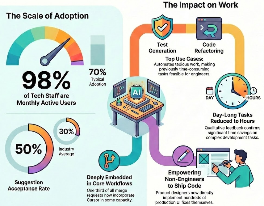
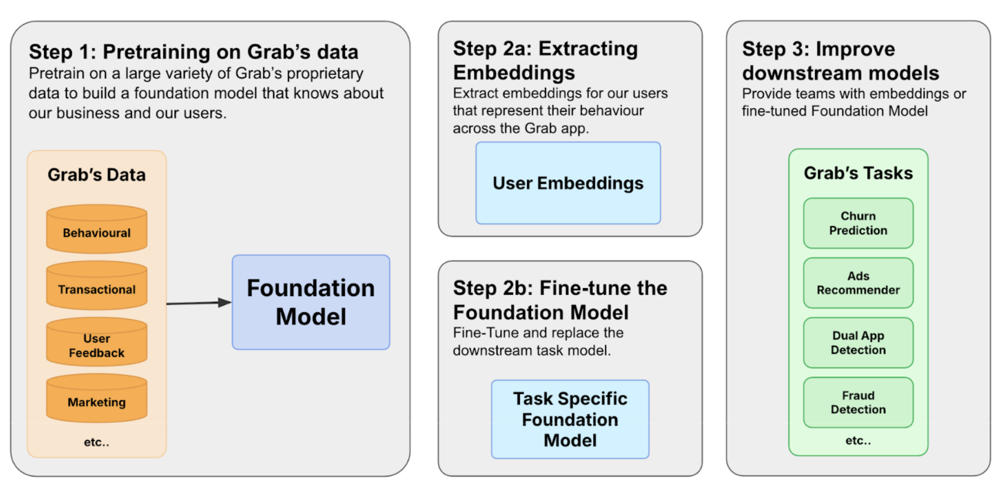
The illustration below encapsulates how Cursor is scaled across Grab, achieving rapid and widespread adoption that accelerated software development and empowered non-technical teams to build solutions.
Figure 1: Adoption overview of AI tool Cursor in Grab.
Multi-tool strategy
Grab embraces a multi-tool strategy for AI coding assistants. Rather than committing to a single solution, we experiment with multiple tools simultaneously, allowing us to compare outcomes and adopt what works. This approach keeps us flexible in a space that evolves quickly. We covered this philosophy in a previous post.
Growth
We introduced Cursor in late 2024 as one of several tools in our AI engineering toolkit. Adoption grew quickly—98% of tech Grabbers became monthly active users, and about 75% use it weekly. For comparison, Google’s 2025 State of AI-Assisted Software Development report highlights that even among high-performing teams, AI coding tool adoption seldom surpasses 70%. Notably, Cursor’s appeal extended beyond engineering, with non-technical teams incorporating it into their workflows.
A standout metric is Cursor’s suggestion acceptance rate, which is around 50%, surpassing the industry average of 30%. This indicates two key insights: first, the suggestions are sufficiently relevant for engineers to accept them half of the time; second, engineers maintain a critical review process rather than accepting suggestions indiscriminately. We attribute this relevance to continuous feedback loops and environment-specific tuning, ensuring suggestions remain aligned with Grab’s codebase and conventions.
Extent of adoption
Raw adoption figures don’t provide the complete picture. We aimed to determine whether engineers were truly incorporating Cursor into their daily workflows or merely experimenting with it sporadically.
The data indicates genuine integration. Approximately half of Cursor users engage with it 10 or more days each month, with some teams achieving full adoption. Over 98% of merge requests now incorporate Cursor in some capacity. Engineers actively share tips and workflows via a dedicated Slack channel, fostering an organic knowledge base.
Across various teams, we’ve observed significant transitions from light usage to moderate and power user levels over the past six months.
Engineer utilization patterns
The most common patterns we see are unit test generation, code refactoring, cross-repository navigation, bug fixing, and automation of routine tasks like API scaffolding or commit messages.
Test generation is particularly popular. Writing tests manually is tedious, and Cursor’s ability to generate and iteratively refine tests has become a standard part of many engineers’ workflows. Cross-repository navigation helps with onboarding and context-switching—engineers can ask Cursor questions about unfamiliar codebases rather than hunting through documentation.
Qualitative feedback confirms what the adoption numbers suggest: tasks that took a full day to complete now take hours. Engineers report tackling refactors and test additions they would have otherwise skipped due to time pressure. Cursor doesn’t just speed up existing work; it makes previously impractical work feasible.
Integration with Grab’s stack
Integrating Cursor effectively at Grab required custom tooling. We built solutions for monorepo indexing to handle Grab’s scale and to distribute preconfigured rules that align Cursor’s suggestions with Grab-specific coding conventions. This integration ensures that Cursor understands our environment rather than offering generic suggestions.
What’s next
Cursor is one tool in a broader toolkit. Our multi-tool strategy means we’re also investing in terminal-based workflows and GrabGPT for internal knowledge retrieval. Different tools suit different workflows. The aim is to empower users, not to restrict them.
Beyond engineering, we’re expanding AI-assisted development to new personas. Our AI Upskilling workshops have trained several hundred Grabbers across five countries, including executive committee members and senior leaders who have built and deployed their own apps. Non-engineers in Financial Planning and Analysis (FP&A), Operations, and regional teams are now building tools with the assitance of AI to solve their own pain points.
Our product design team has launched an initiative empowering designers to directly implement production fixes. Designers have successfully merged hundreds of merge requests, often with same-day turnaround, facilitating quicker iterations on UI fixes without the engineering queue delay. This process requires designers to be trained in Git fundamentals prior to gaining access, with initial reviews conducted by design managers.
Cursor has become part of daily work at Grab. But adoption is only half the question — the other half is impact. We’ve been running a parallel effort to measure productivity effects rigorously, using fixed-effects regression to isolate Cursor’s contribution from other factors. Early findings show a dose-response relationship: productivity gains scale with usage intensity, and the effects hold up to statistical scrutiny.
We will address the measurement methodology and present our findings in a subsequent post.
Join us
Grab is a leading superapp in Southeast Asia, operating across the deliveries, mobility and digital financial services sectors. Serving over 800 cities in eight Southeast Asian countries, Grab enables millions of people everyday to order food or groceries, send packages, hail a ride or taxi, pay for online purchases or access services such as lending and insurance, all through a single app. Grab was founded in 2012 with the mission to drive Southeast Asia forward by creating economic empowerment for everyone. Grab strives to serve a triple bottom line – we aim to simultaneously deliver financial performance for our shareholders and have a positive social impact, which includes economic empowerment for millions of people in the region, while mitigating our environmental footprint.
Powered by technology and driven by heart, our mission is to drive Southeast Asia forward by creating economic empowerment for everyone. If this mission speaks to you, join our team today!
At Grab, we’ve been exploring ways to dramatically reduce container startup times for our data platforms. Large container images for services like Airflow and Spark Connect were taking minutes to download, causing slow cold starts and poor auto-scaling performance. This blog post shares our journey implementing Docker image lazy loading using eStargz and Seekable OCI (SOCI) technologies, the results we achieved, and the lessons learned along the way.
Results: The numbers speak for themselves
Benchmark results
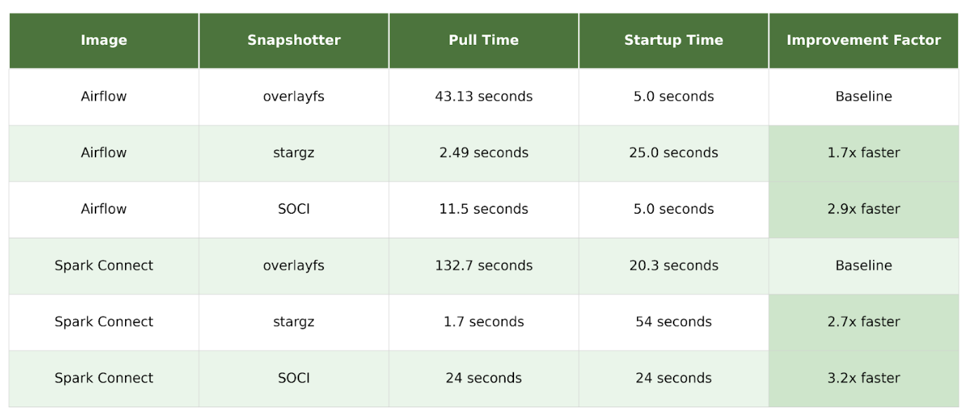
Our initial testing on fresh nodes (nodes without cached images) showed dramatic improvements in image pull times as shown in Figure 1.
Figure 1. Table of results.
The key advantage of lazy loading is the reduction in image pull time, especially on “fresh” nodes that do not have the image cached. By analyzing detailed pod events, we can see the precise impact of using the stargz snapshotter.
During our SOCI benchmark testing, we observed an important distinction between SOCI and eStargz: SOCI maintains the same application startup time as standard images, while eStargz takes longer. For example, with Airflow, both overlayFS and SOCI achieved 5.0 seconds startup time, while eStargz took 25.0 seconds. This demonstrates that lazy loading doesn’t eliminate download time; it redistributes it. SOCI’s approach of maintaining separate indexes allows it to optimize the download-to-startup time trade-off more effectively, keeping application startup performance on par with standard images while still dramatically reducing image pull time.
Production performance
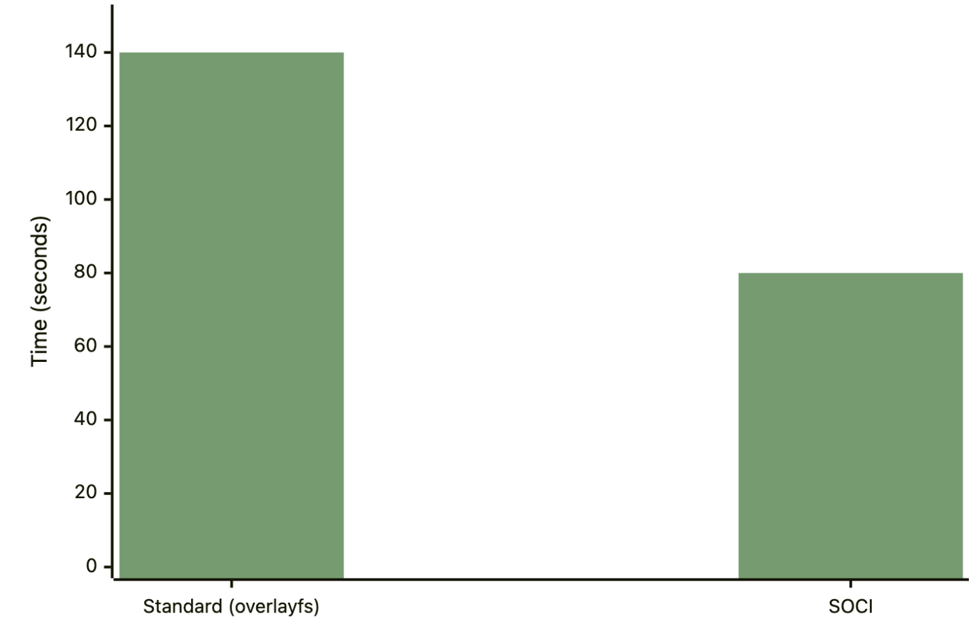
The production deployment of SOCI lazy loading has delivered significant, measurable improvements across our data platforms. Both Airflow and Spark Connect now experience 30-40% faster startup times, directly improving our ability to handle traffic spikes and scale efficiently. These improvements translate to better auto-scaling responsiveness, reduced resource waste during initialization, and improved user experience for data processing workloads. The sustained performance gains observed over time demonstrate that lazy loading is a stable, production-ready optimization that delivers consistent value.
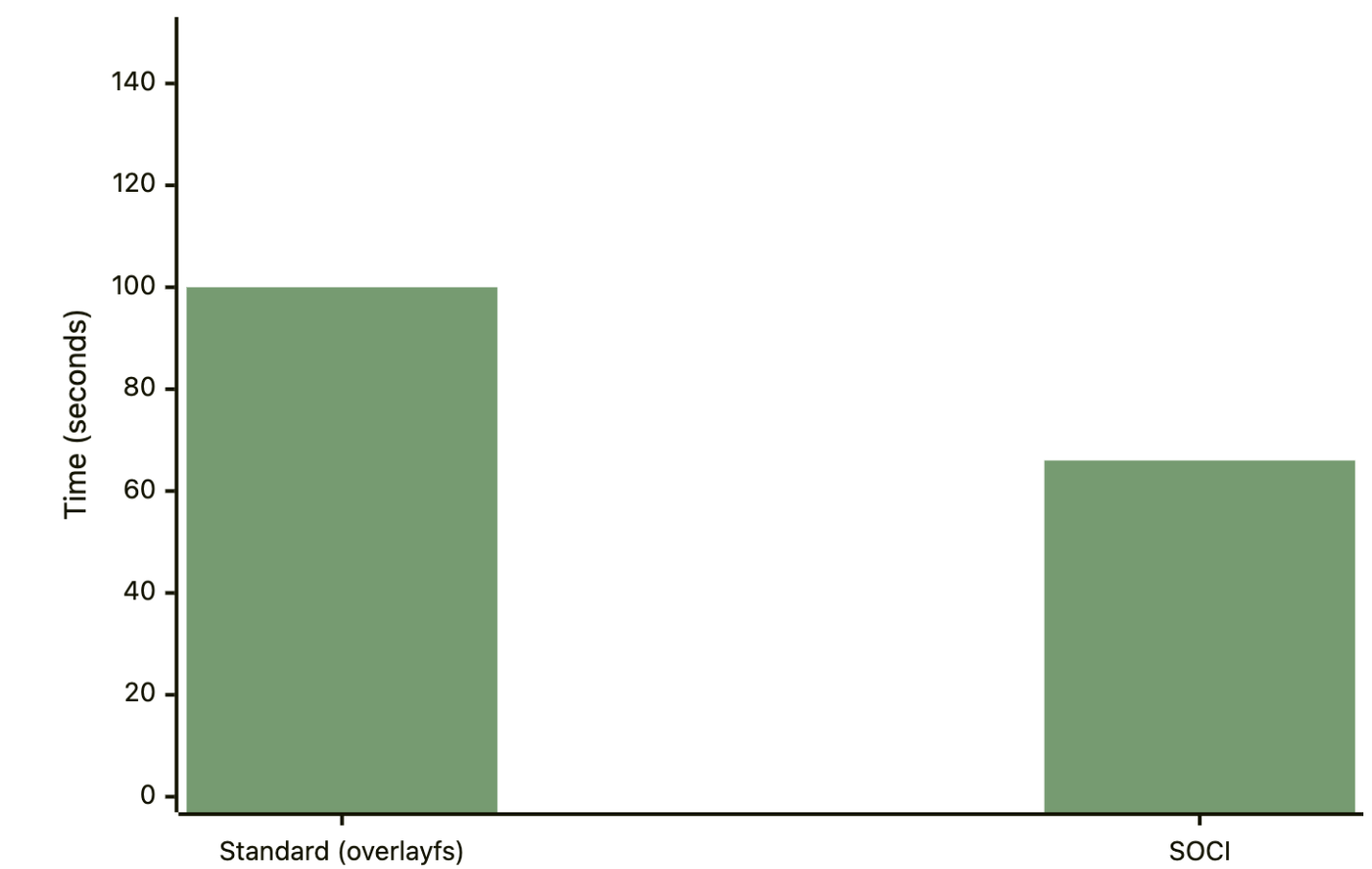
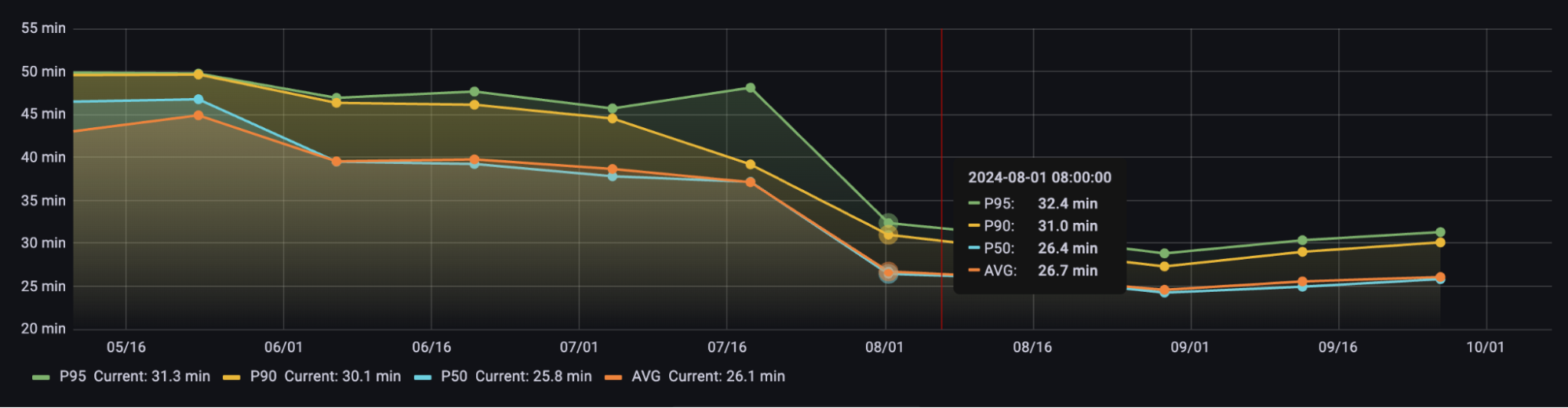
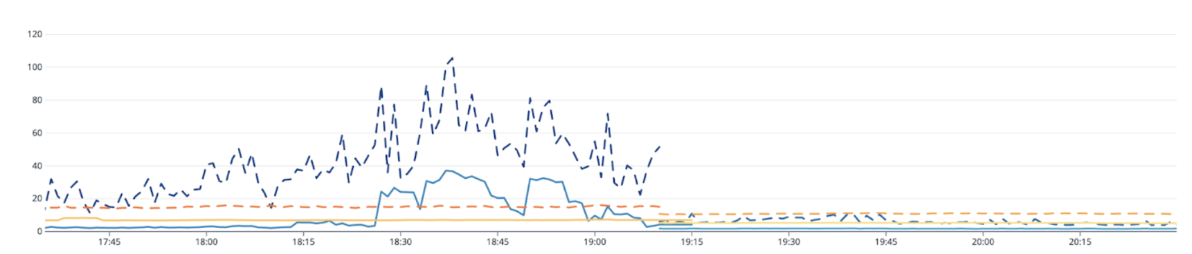
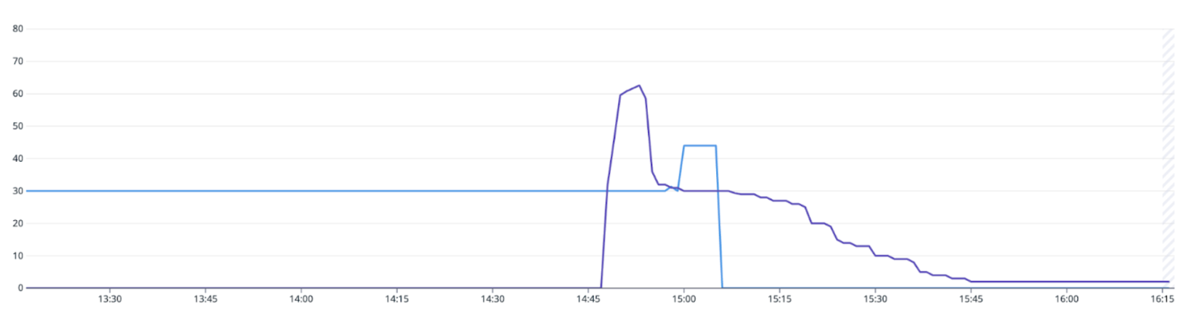
Figure 2 and 3 illustrates the P95 startup time improvements for both services:
Figure 2. Production results: Airflow P95 startup time.
Figure 3. Production results: Spark Connect P95 startup time.
It is important to note that P95 startup time includes both the image download/pull time and the application startup time itself. This metric captures the entire system performance for both cold and hot starts on fresh and hot nodes, showing the overall system improvement rather than just cold start performance.
During the production deployment and monitoring, we gained valuable insights on SOCI configuration tuning. Following AWS’s recommended configuration from their blog on Introducing Seekable OCI: Parallel Pull Mode for Amazon EKS, we optimized our SOCI snapshotter settings:
Increased max_concurrent_downloads_per_image from 5 to 10.
Increased max_concurrent_unpacks_per_image from 3 to 10.
Increased concurrent_download_chunk_size from 8MB to 16MB (aligning with AWS’s recommendation for Elastic Container Registry (ECR)).
This configuration tuning led to a significant performance improvement: image download time on a fresh node was reduced from 60 seconds to 24 seconds, representing a 60% improvement. The key lesson here is that default SOCI configurations may not be optimal for all environments, and tuning these parameters based on your infrastructure (especially when using ECR) can yield substantial gains.
Technical background: How Docker lazy loading works
Container root filesystem (rootfs) and file organization
A container’s root filesystem, or rootfs, is the directory structure that the container sees as its root (/). It contains all the files and directories necessary for an application to run, including the application itself, its dependencies, system libraries, and configuration files. It’s an isolated filesystem, separate from the host machine’s filesystem.
The rootfs is built from a series of read-only layers that come from the container image. Each instruction in an image’s Dockerfile creates a new layer, representing a set of filesystem changes. When a container is launched, a new writable layer, often called the “container layer,” is added on top of the stack of read-only image layers. Any changes made to the running container, such as writing new files or modifying existing ones, are written to this writable layer. The underlying image layers remain untouched. This is known as a copy-on-write (CoW) mechanism.
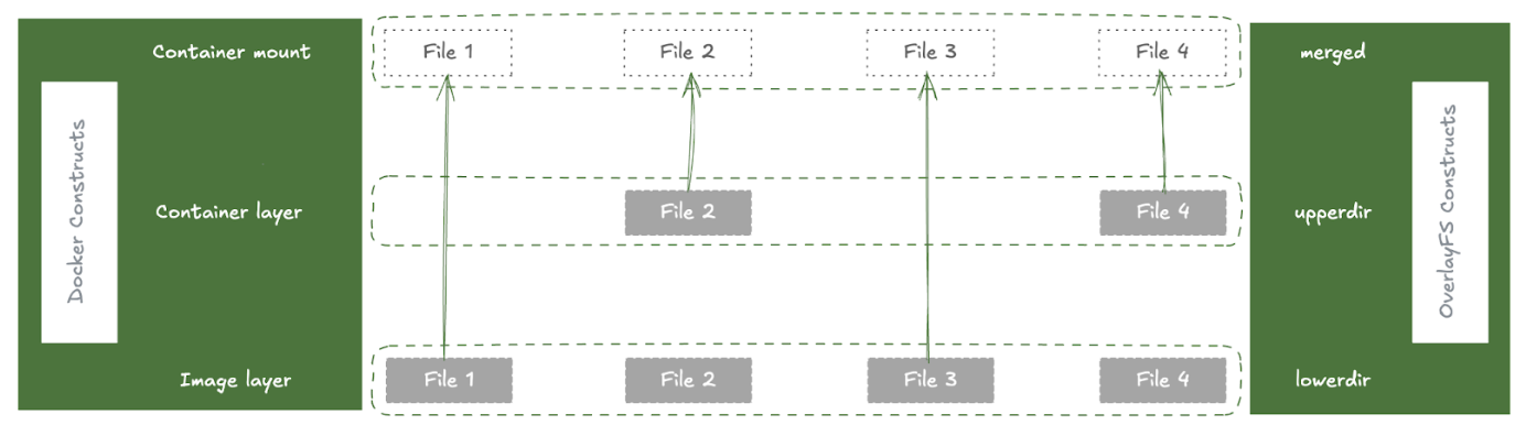
In containerd, a snapshotter is a plugin responsible for managing container filesystems. Its primary job is to take the layers of an image and assemble them into a rootfs for a container. The default snapshotter in containerd is overlayFS, which uses the Linux kernel’s OverlayFS driver to efficiently stack layers. To assemble the rootfs, the overlayFS snapshotter creates a “merged” view of the read-only image layers:
Figure 4. How OverlayFS assembles the container filesystem.
lowerdir: The read-only image layers are used as the lowerdir in OverlayFS. These are the immutable layers from the container image.
upperdir: A new, empty directory is created to be the upperdir. This is the writable layer for the container where any changes are stored.
merged: The merged directory is the unified view of the lowerdir and upperdir. This is what is presented to the container as its rootfs.
When a container reads a file, it’s read from the merged view. When a container writes a file, it’s written to the upperdir using a copy-on-write mechanism. This is an efficient way to manage container filesystems, as it avoids duplicating files and allows for fast container startup.
The problem: Traditional container image pull
To understand the benefits of lazy loading, we first need to understand the traditional container image pull process:
Download layers: The container runtime downloads all layer tarballs that make up the image.
Unpack layers: Each layer is unpacked and extracted onto the host’s disk.
Create snapshot: The snapshotter combines these layers into a single, unified filesystem, known as the container’s rootfs.
Start container: Only after all layers are downloaded and unpacked can the container start.
This process is slow, especially for large images, as the entire image must be present on the host before the container can launch.
The solution: Remote snapshotter
To address the slow startup issue with large images, we use a remote snapshotter solution. A remote snapshotter is a special type of snapshotter that doesn’t require all image data to be locally present. Instead of downloading and unpacking all the layers, it creates a “snapshot” that points to the remote location of the data (like a container registry). The actual file content is then fetched on-demand when the container tries to read a file for the first time.
While a traditional snapshotter like overlayFS uses directories on the local disk as its lowerdir, a remote snapshotter creates a virtual lowerdir that is backed by the remote registry. This is typically done using FUSE (Filesystem in Userspace). The remote snapshotter creates a FUSE filesystem that presents the contents of the remote layer as if it were a local directory. This FUSE mount is then used as the lowerdir for the overlayFS driver. This allows the remote snapshotter to integrate with the existing overlayFS infrastructure while adding the capability of lazy-loading data from a remote source.
There are two main formats that enable remote snapshotters: eStargz and SOCI.
eStargz format
eStargz is a backward-compatible extension of the standard OCI tar.gz layer format. It has several key features that enable lazy loading:
Individually compressed files: Each file within the layer (and even chunks of large files) is compressed individually. This is the key that allows for random access to file contents.
TOC (table of contents): A JSON file named stargz.index.json is located at the end of the layer. This TOC contains metadata for every file, including its name, size, and, most importantly, its offset within the layer blob.
Footer: A small footer at the very end of the layer contains the offset of the TOC, allowing it to be easily located by reading only the last few bytes of the layer.
Chunking and verification: Large files can be broken down into smaller chunks, each with its own entry in the TOC. Each chunk also has a chunkDigest in its TOC entry, allowing for independent verification of each downloaded piece of data.
Prefetch landmark: A special file, .prefetch.landmark, can be placed in the layer to mark the end of “prioritized files”. This allows the snapshotter to intelligently prefetch the most important files for the container’s workload.
The stargz snapshotter uses the eStargz format to enable lazy loading. Here’s how it works:
Mount request: When containerd calls the Mount function, it’s the main entry point for creating a new filesystem for a layer.
Resolve and read TOC: The snapshotter fetches the layer’s footer, then fetches the stargz.index.json TOC from the remote registry. This TOC contains all the file metadata needed to create a virtual filesystem.
Mount FUSE filesystem: With the TOC in memory, the snapshotter creates a virtual filesystem using FUSE. The container can now start, as it has a valid rootfs, even though most of the file content has not been downloaded.
On-demand fetching: When the container performs a file operation like read(), the FUSE filesystem intercepts the call. The snapshotter checks a local disk cache for the requested bytes. If the data is not cached, it issues an HTTP Range request to the container registry to download only the required chunk of the layer.
Remote fetching and caching: The downloaded data is returned to the container and also written to the local cache for subsequent reads.
Prefetching for optimization: After the FUSE filesystem is mounted, a background goroutine begins downloading the prioritized files (up to the .prefetch.landmark) and can also be configured to download the entire rest of the layer in the background.
SOCI is a technology open sourced by AWS that enables containers to launch faster by lazily loading the container image. SOCI works by creating an index (SOCI Index) of the files within an existing container image. SOCI borrows some of the design principles from stargz-snapshotter but takes a different approach:
Separate index: A SOCI index is generated separately from the container image and is stored in the registry as an OCI Artifact, linked back to the container image by OCI Reference Types.
No image conversion: This means that the container images do not need to be converted, image digests do not change, and image signatures remain valid.
Native Bottlerocket support: SOCI is natively supported on Bottlerocket OS.
When using EKS with containerd as the container runtime, you can configure remote snapshotters to enable lazy loading. Here’s how to set them up:
For stargz-snapshotter (eStargz): You need to install the containerd-stargz-grpc service first, then register it as a proxy plugin in containerd’s configuration:
# /etc/containerd/config.toml
[proxy_plugins]
[proxy_plugins.stargz]
type = "snapshot"
address = "/run/containerd-stargz-grpc/containerd-stargz-grpc.sock"
For detailed installation instructions, see the stargz-snapshotter installation documentation. The setup can be baked into an AMI for production use or tested via user data from node bootstrap scripts.
For SOCI snapshotter (Bottlerocket): On Bottlerocket nodes, enable the SOCI snapshotter via user data:
SOCI doesn’t require rebuilding images; you only need to generate a SOCI index for existing images. Since Docker doesn’t natively support SOCI index generation yet, workaround solutions include using the AWS SOCI Index Builder Using Lambda Functions or integrating SOCI index generation into your CI/CD pipeline as described in this blog post.
Key takeaway: Why we chose SOCI
We started our exploration with eStargz but ultimately chose SOCI for production deployment. The key reason is scalability and alignment with our strategy to use Bottlerocket OS for enhancing Kubernetes pod startup and security. SOCI is natively supported by Bottlerocket, which means service teams don’t need to set up and maintain the more complicated stargz snapshotter across all EKS clusters. This makes the implementation easier to maintain and provides better support from AWS.
Additionally, we learned that lazy loading doesn’t eliminate the time required to download image data; it redistributes it from startup time to runtime. While this dramatically improves cold start performance, it’s important to monitor application performance closely and tune configuration parameters based on your workload and infrastructure. We achieved a 60% improvement by optimizing SOCI’s parallel pull mode settings, demonstrating the value of proper configuration tuning.
Conclusion
Docker image lazy loading with SOCI offers a significant opportunity to improve the performance and efficiency of our services at Grab. Our testing and production deployments have shown:
4x faster image pull times on fresh nodes.
29-34% improvement in P95 startup times for production workloads.
60% improvement in image download times with proper configuration tuning.
The implementation path is clear, low-risk, and builds on proven components. This technology is production-ready, and we’re continuing to scale it across more services.
Grab is a leading superapp in Southeast Asia, operating across the deliveries, mobility and digital financial services sectors. Serving over 800 cities in eight Southeast Asian countries, Grab enables millions of people everyday to order food or groceries, send packages, hail a ride or taxi, pay for online purchases or access services such as lending and insurance, all through a single app. Grab was founded in 2012 with the mission to drive Southeast Asia forward by creating economic empowerment for everyone. Grab strives to serve a triple bottom line – we aim to simultaneously deliver financial performance for our shareholders and have a positive social impact, which includes economic empowerment for millions of people in the region, while mitigating our environmental footprint.
Powered by technology and driven by heart, our mission is to drive Southeast Asia forward by creating economic empowerment for everyone. If this mission speaks to you, join our team today!
You’ve vibe-coded an AI assistant that’s a game-changer for your team. It works perfectly on your laptop. But when you try to deploy it company-wide, everything falls apart.
This is what is known as “deployment slop”—the messy reality when quick AI prototypes hit the enterprise world. Your tool suddenly becomes unreliable, insecure, and impossible to maintain. Different teams run different versions. Security flags it. IT won’t touch it. Your innovation dies.
BriX solves this. It’s a platform that takes your working AI prototype and makes it production-ready—without forcing you to become a full-stack developer. BriX handles the hard parts such as security, scaling, and data connections, so you can focus on building great tools. Switch between AI models like Claude or GPT with a click. Connect securely to your company’s data sources. Deploy once, and it just works—for everyone.
This article shows how BriX transforms AI deployment from an engineering bottleneck into a configuration task, enabling domain experts to ship enterprise-grade AI tools in days instead of months.
Introduction
Building AI tools has never been easier. With ChatGPT, Claude, and other Large Language Models (LLMs), anyone can prototype a useful AI assistant in an afternoon. Data analysts build metric query tools; product managers create research assistants. This rapid experimentation—”vibe coding”—has sparked innovation across organizations.
But then comes the hard part: deployment.
That brilliant tool you built on your laptop? It works great for you. But when your boss asks you to “roll it out to the whole company,” you hit a wall. Suddenly you need:
Security reviews (Is it leaking sensitive data?)
Reliability guarantees (What happens when 500 people use it at once?)
Access controls (Who can see what data?)
Audit trails (Who asked what, and when?)
Consistent behavior (Why does it give different answers to different people?)
Most builders aren’t DevOps engineers. They’re domain experts who had a good idea. So these tools either:
Never get deployed (innovation dies in a Jupyter notebook); or
Get deployed badly (creating “Deployment Slop”—a mess of insecure, unreliable scripts).
The three failure modes of deployment slop
The chaos problem: Everyone’s running a different version
Marketing copies your script and tweaks the prompts. Finance changed the model from GPT-4 to Claude because it’s cheaper. Sales adds their own data sources. Within weeks, you have:
Five different versions of “the same tool”.
Wildly different answers to the same question.
No one knows which version is “correct”.
Teams making decisions based on inconsistent data.
Potential risk: A senior executive receiving conflicting answers from different teams, resulting in a loss of trust.
The reliability problem: It works until it doesn’t
Your laptop script was built for one user (you). Now 50 people are using it simultaneously. The result:
Timeouts and crashes during peak hours.
No error handling (users see cryptic Python stack traces).
Rate limits hit on API calls.
No monitoring or alerts when things break.
You become the “on-call” support person for a side project.
Potential risk: The tool fails during a critical metric review leaving folks to find the solution manually.
The security problem: Accidental data leaks
Your prototype connects directly to production databases. It has your personal credentials hardcoded. There’s no:
Access control (everyone sees all data, including sensitive info).
Audit trail (no record of who queried what).
Data governance (PII might be exposed).
Compliance review (legal and security teams don’t even know it exists).
Potential risk: An employee inadvertently querying PII, resulting in a potential breach.
Who gets hit hardest?
This problem is especially painful for semi-technical builders—the domain experts who understand the business problem but aren’t DevOps engineers:
Product Managers who write SQL but not Kubernetes configs.
Data Analysts who know Python but not cloud security.
Marketing Ops who build dashboards but not CI/CD pipelines.
HR Analytics who understand people data but not infrastructure scaling.
The traditional solution is to “hand it to Engineering,” but they are backlogged for months. By the time they rebuild your tool “properly,” the business need has changed.
Solution: Enter BriX: From prototype to production in days, not months
BriX is a platform that solves the deployment problem by centralizing all the hard infrastructure work. Instead of forcing every builder to become a DevOps expert, BriX provides the production-ready foundation so you can focus on building great AI tools.
The core insight: Deployment doesn’t have to be an engineering problem. It can be a configuration problem.
What BriX does
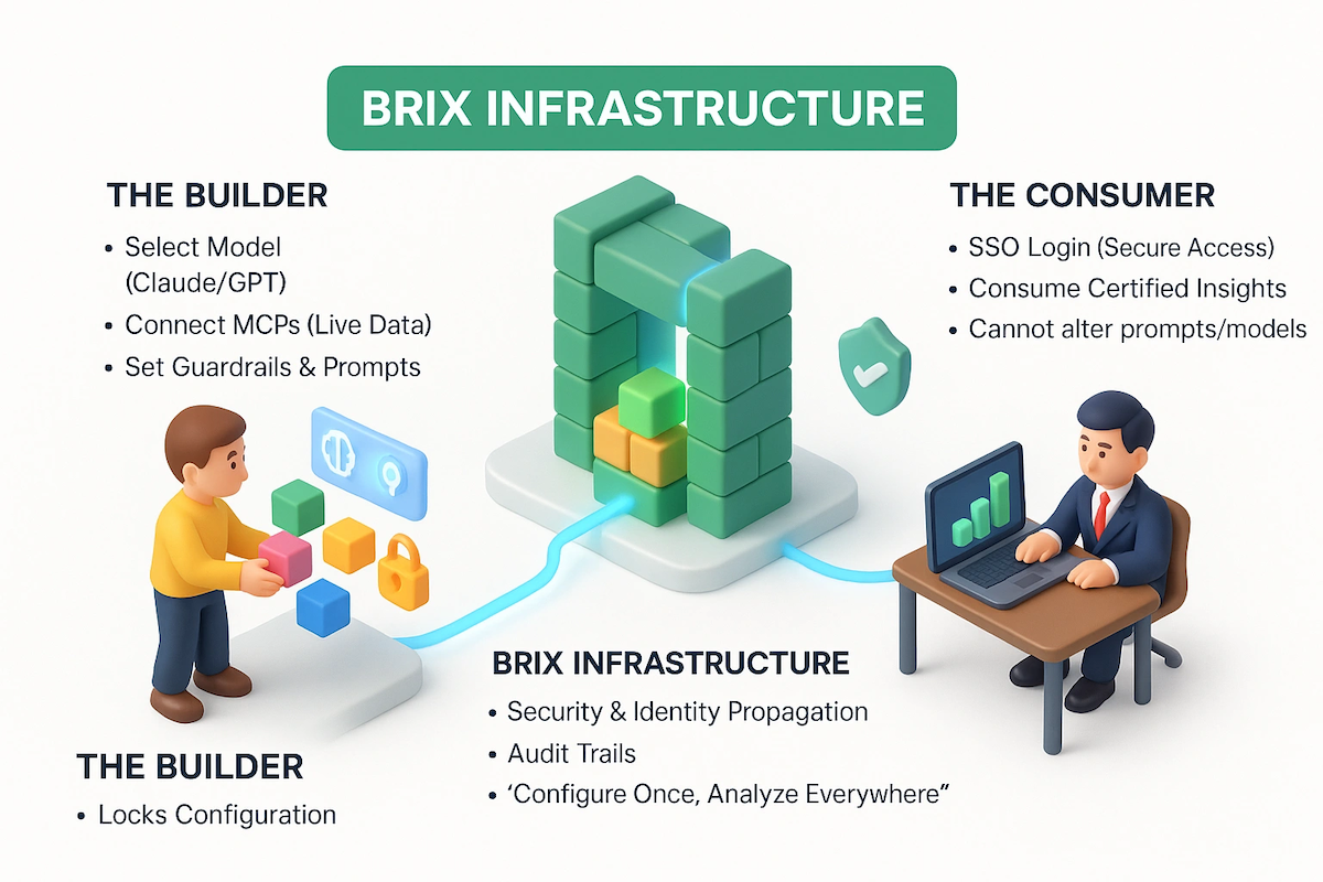
Think of BriX as the “production layer” for AI tools. You bring your working prototype. BriX handles security, scaling, data connections, monitoring, audit trails, and consistent behavior across teams.
You configure. BriX deploys.
Figure 1. BriX infrastructure
The three core capabilities
Choose your AI model (Model agnosticism)
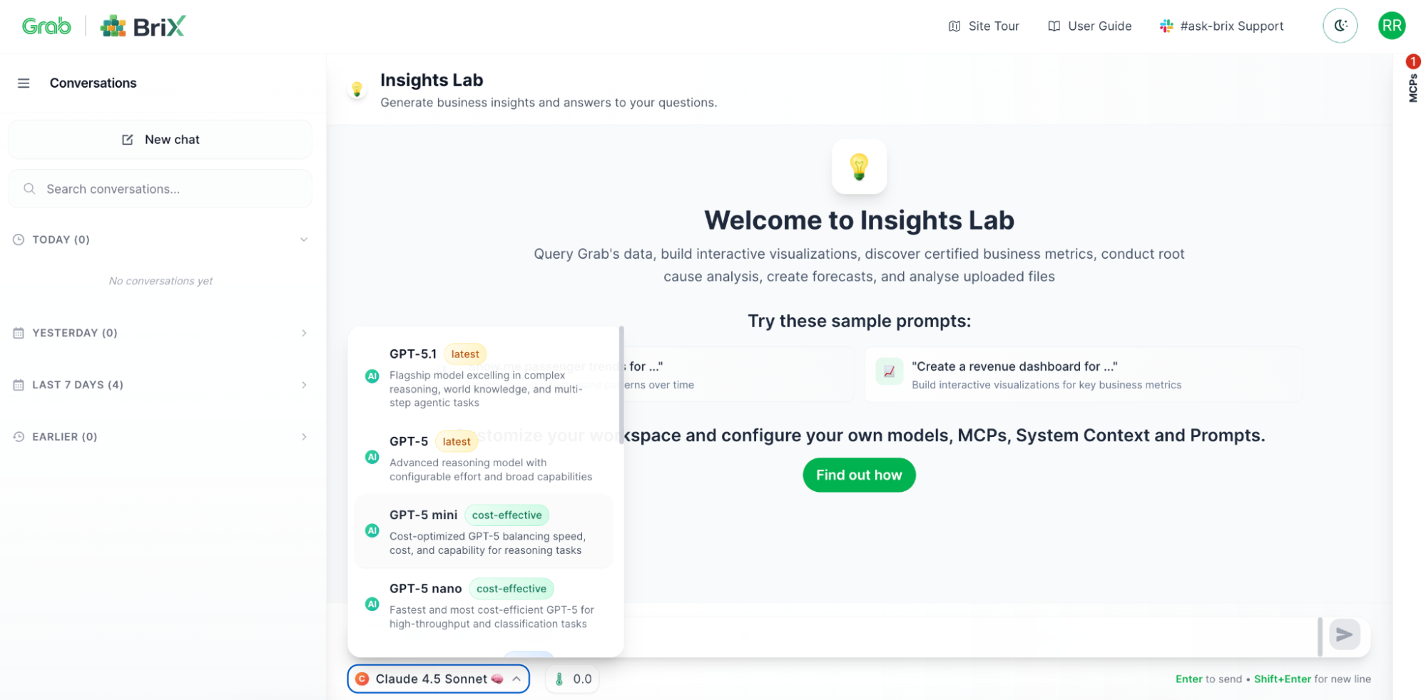
Different tasks need different models. BriX lets you switch between models with a dropdown—Claude, GPT, Gemini, or others. Test which works best. Change models without rewriting code. Optimize for cost vs. performance.
Example: Your finance tool uses GPT-4 for complex analysis, but a new better model is available. Change it in BriX with one click—no code changes needed.
Figure 2. Model selection interface
Connect to enterprise data securely (Model Context Protocols)
This is where BriX really shines. Your AI tool needs data—metrics, customer info, documentation. But connecting to enterprise systems securely is hard.
Model Context Protocols (MCPs) are BriX’s solution. Think of them as secure, pre-built connectors to your company’s data sources.
Why MCPs matter:
Security built-in: No hardcoded credentials, proper access controls.
Certified data: Connect only to approved, governed data sources.
No custom integration: Pre-built connectors, not custom API code.
Audit trails: Every query is logged automatically.
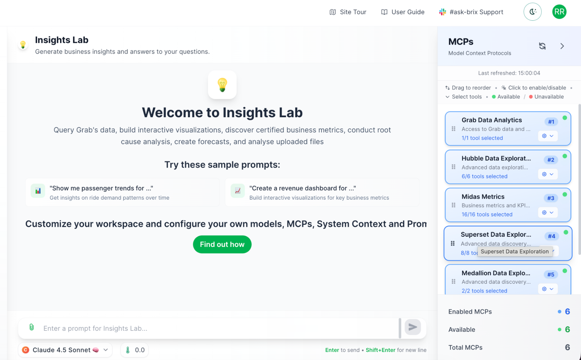
Example: Your marketing tool can query the metrics system to get conversion rates, search the knowledge base for campaign guidelines, and pull customer data from the data lake —all through secure, governed connections.
Technical note: MCPs use a standardized protocol, so adding new data sources doesn’t require rebuilding your tool. BriX handles the complexity.
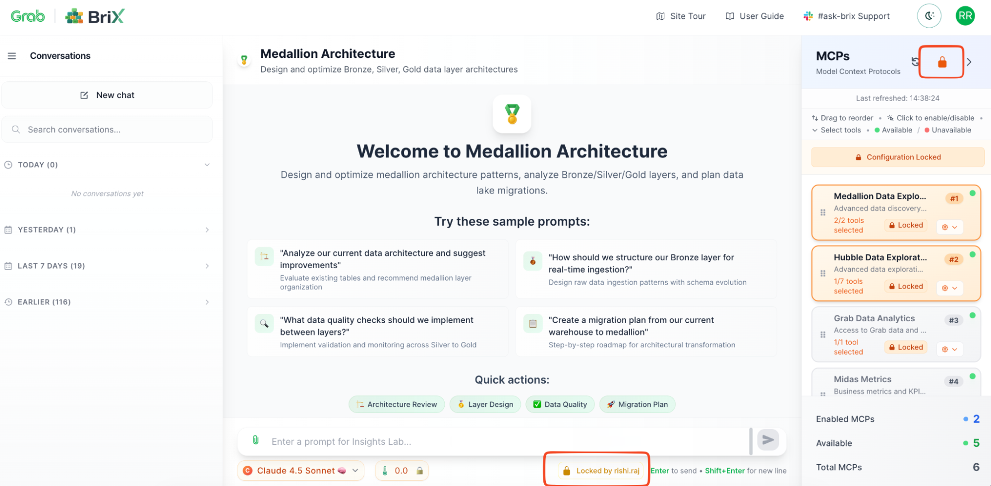
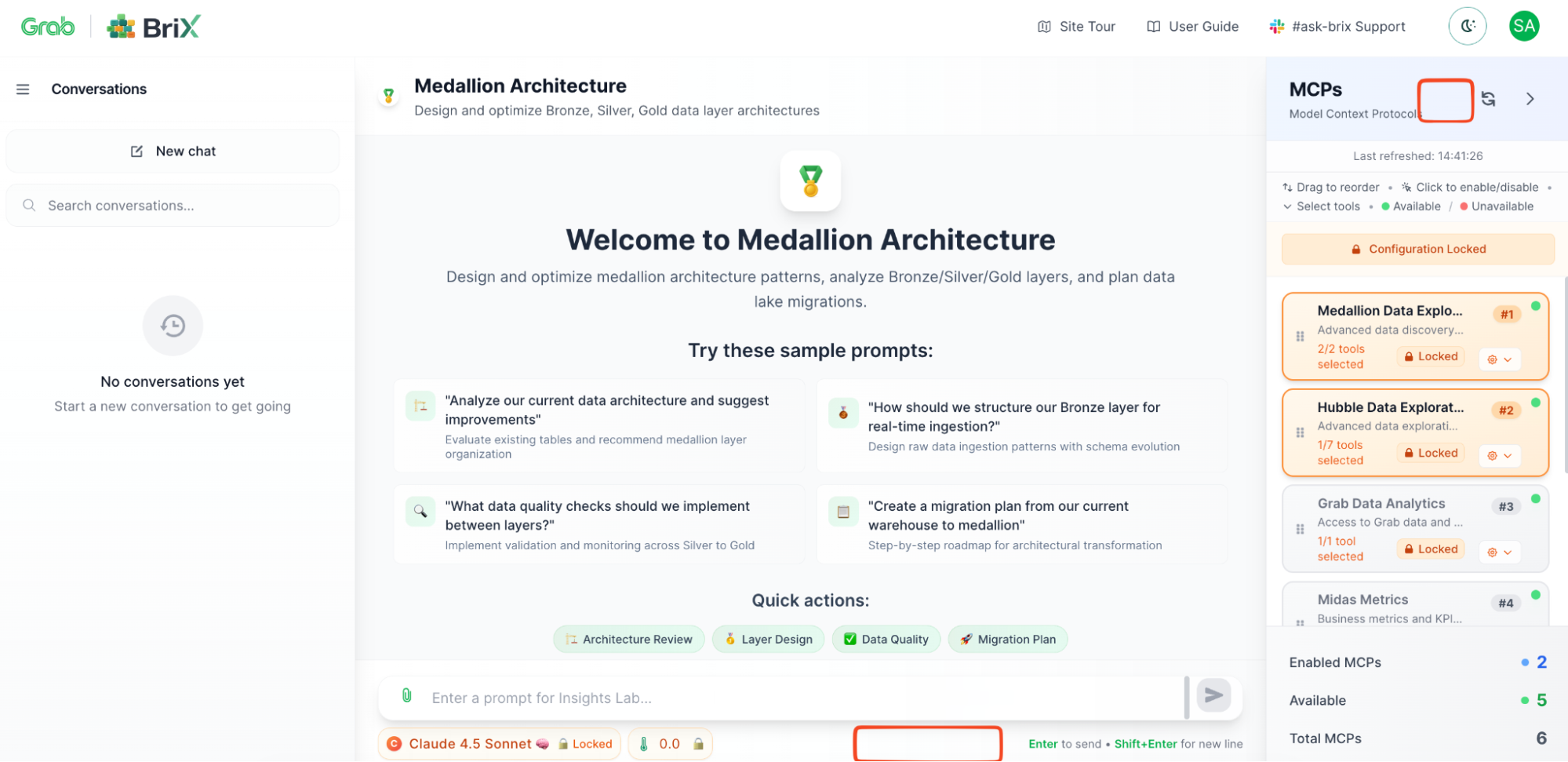
Figure 3. BriX chat user interface
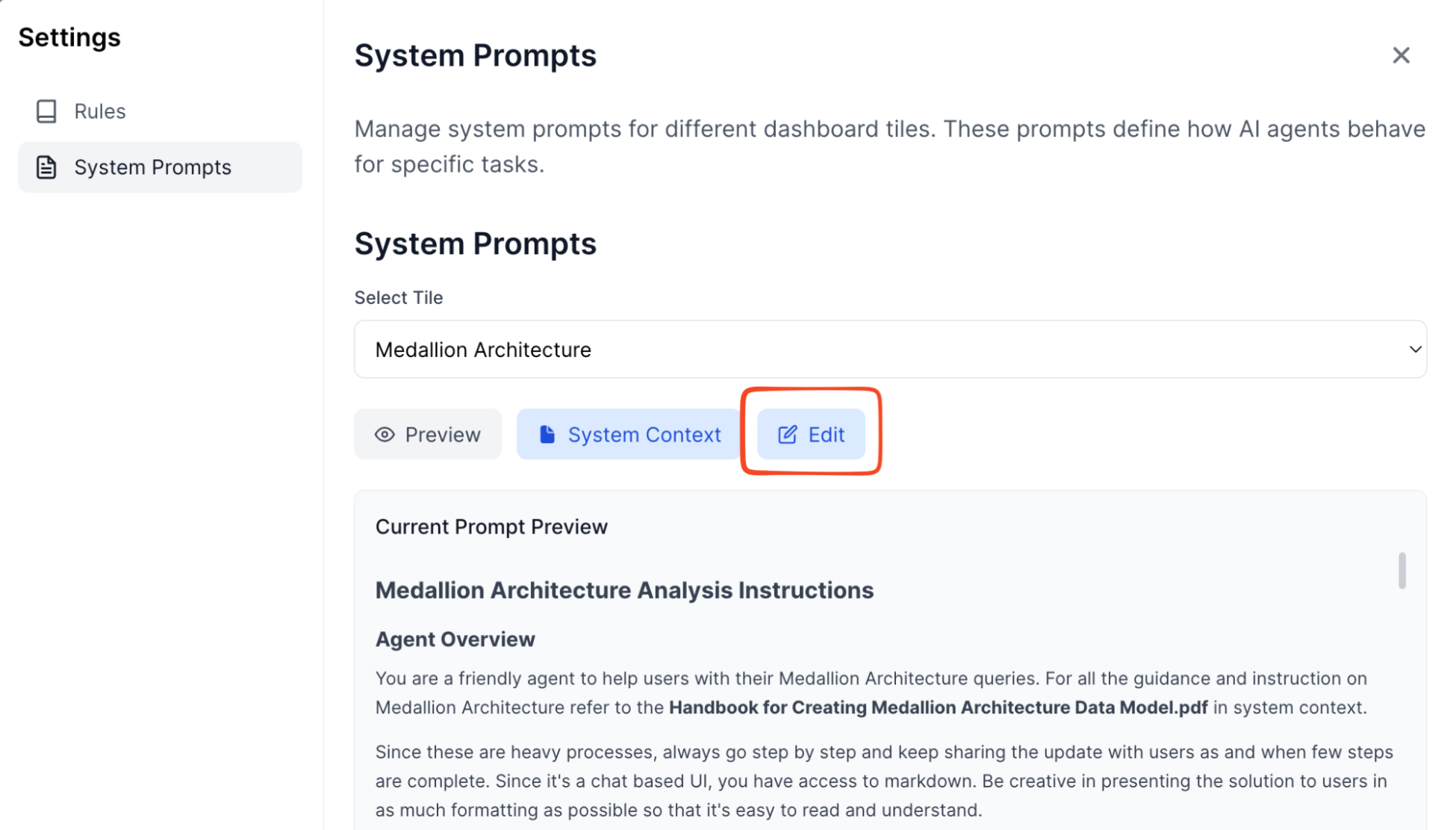
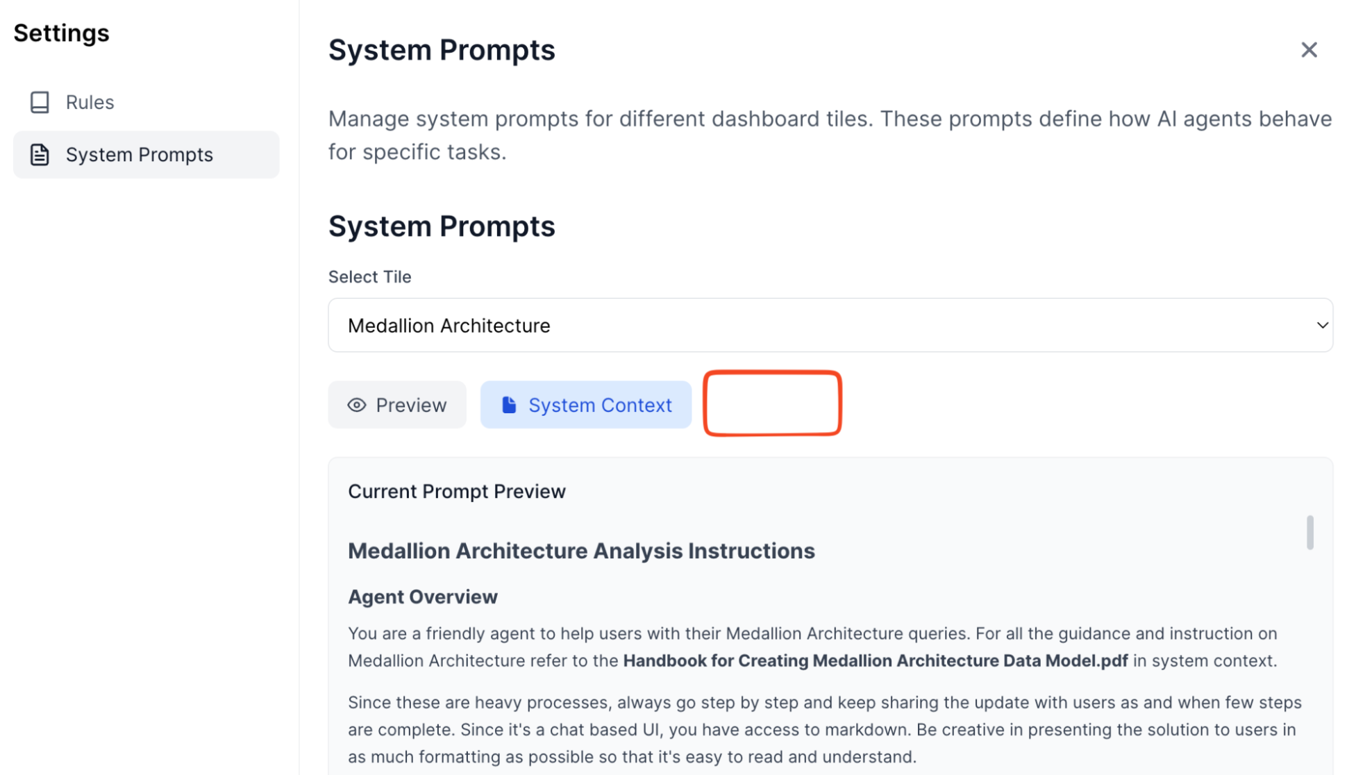
Ensure consistent behavior (System prompts and context)
Remember the “chaos problem” where everyone runs different versions? BriX solves this with centralized configurations by allowing you to lock it down for the users:
System prompts: Define your AI’s personality, tone, and guardrails once.
Context files: Upload reference documents that every instance uses.
Global enforcement: All users get the same behavior automatically.
Example: Your customer support tool has a system prompt that says “Always be empathetic, never make promises about refunds, escalate to humans for complaints.” Every support agent’s AI follows these rules—no exceptions.
Figure 4. The builder’s view
Additional feature: Flexible interfaces and collaboration
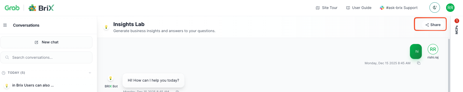
Beyond the core infrastructure, BriX offers flexible ways to consume these tools. BriX goes beyond conversational interfaces—you can host custom UIs built with any frontend framework while BriX handles the AI backend. Users can also generate and share analyses as persistent reports, turning individual queries into institutional knowledge accessible across teams via shareable links—complete with data, visualizations, and AI insights.
Figure 5. Share feature interface
The BriX workflow: A real example
Let’s see how a product manager would use BriX:
Step 1: Upload your prototype
You’ve built a Jupyter notebook that queries metrics and generates reports.
Upload it to BriX (or connect your GitHub repo).
Step 2: Configure (Not code)
Choose your AI model: Claude 4.5 Sonnet
Connect data sources: Midas (metrics), Hubble (data lake)
Set system prompt: “You’re a data analyst. Always cite sources. Format numbers with commas.”
Upload context: Your company’s metrics definitions guide.
Step 3: Lock
Lock all the configurations of your BriX.
Share with your team.
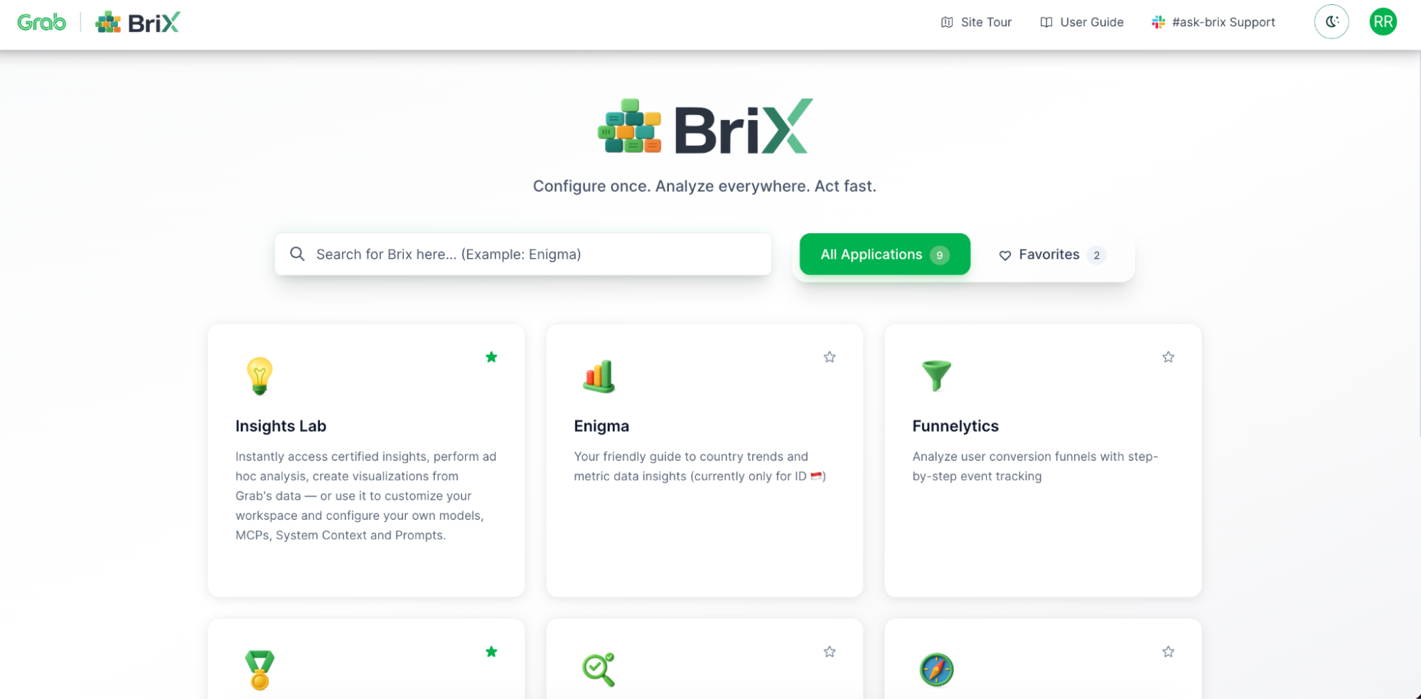
Figure 6. BriX landing page
Figure 7. The user’s view (Locks and edit not available)
Step 4: It just works
Certification by design with Brick Quality residing with the brick admin.
Focused use cases have specific system prompts, context – minimizing hallucination concerns.
People can use it simultaneously (BriX handles scaling).
Everyone gets consistent answers (same model, same prompts).
All queries are logged (audit trail automatic).
The security team is happy (proper access controls).
You’re not on-call (BriX monitors and alerts).
Time to production: 3 Days, not 3 months.
Under the hood: The BriX architecture
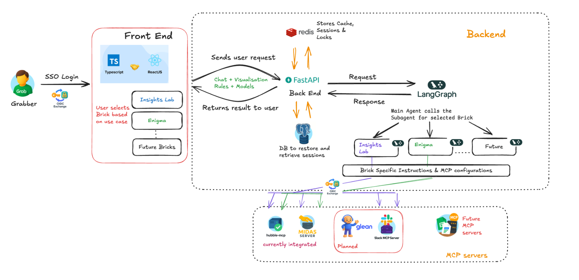
BriX is built on a synchronous streaming architecture—a design that prioritizes real-time responsiveness without sacrificing enterprise security. Think of it like a live sports broadcast: you see the action as it happens, not a delayed replay.
Figure 8. BriX architecture
Here’s how a single user request flows through the system, from question to answer.
The request journey: Six layers
User Question
      ↓
[1] The Frontend — Real-Time Streaming
      ↓
[2] The Gateway — FastAPI Backend
      ↓
[3] The Brain — LangGraph Orchestration
      ↓
[4] Memory — Hot and Cold Storage
      ↓
[5] Security — Identity Propagation ("On-Behalf-Of" Flow)
      ↓
[6] Data Processing — Full Context, Not Fragments
      ↓
Response streams back to user in real-time
Let’s break down each layer.
Layer 1: The frontend — Real-time streaming
Technology: React (TypeScript)
User experience: ChatGPT-style interface
The User types a question: “What’s our conversion rate in Singapore last month?”
The frontend opens a persistent connection to BriX servers. As the AI processes the question, updates stream back instantly:
“🤔 Thinking…”
“📊 Querying metrics database…”
“✅ Found 3 relevant data points…”
[Final answer appears]
Why streaming matters:
Traditional approach
BriX approach
❌ User waits 30 seconds, sees nothing, then gets full answer (feels broken).
✅ User sees progress every second (feels responsive and trustworthy).
Technical implementation: Server-Sent Events (SSE) for real-time updates without WebSocket complexity.
Layer 2: The Gateway — FastAPI backend
Technology: FastAPI (Python)
Role: Central traffic controller
What it does:
Receives all incoming requests
Authenticates users (checks SSO tokens)
Routes requests to the appropriate agent
Manages rate limiting (prevents abuse)
Handles errors gracefully
Why FastAPI?
⚡ Fast (async/await for concurrent requests)
🔒 Secure (built-in authentication)
📈 Scalable (handles thousands of concurrent users)
Layer 3: The Brain — LangGraph orchestration
Technology: LangGraph (AI workflow framework)
Role: The “main agent” that coordinates everything.
Think of LangGraph as a smart router that understands intent and delegates work.
Example flow:
User asks: “Compare our Singapore and Malaysia conversion rates, then explain why they differ”.
This is where BriX’s security model shines. Instead of using a single “service account” to access all data, BriX uses your credentials for every query.
How it works:
Step 1: Authentication (Login)
You log in via SSO (e.g., Okta, Azure AD)
BriX receives a secure token that represents your identity
This token includes your permissions (what data you can access)
Step 2: Identity propagation (Query execution)
You ask: “Show me customer revenue data”
BriX doesn’t use its own credentials to query the database
Instead, BriX carries your token to the data source
The data source checks: “Does this user have permission to see revenue data?”
If yes → Returns data
If no → Access denied
Step 3: Audit trail
Every query is logged with:
Who asked (your user ID)
What they asked (the question)
What data was accessed (the query)
When it happened (timestamp)
Why this matters:
Traditional approach
BriX approach
❌ Service account has access to ALL data.
✅ Each user only sees their authorized data.
❌ Can’t tell who accessed what.
✅ Complete audit trail per user.
❌ Security team nervous about AI tools.
✅ Security team approves (same controls as existing tools).
❌ One compromised credential = full breach.
✅ Breach limited to single user’s permissions.
Real-world example:
Finance analyst asks about revenue → Sees all financial data (authorized)
Marketing analyst asks same question → Sees only marketing budget (restricted)
Same AI tool, different permissions → Security enforced automatically
Technical term: This is called “identity propagation” or “on-behalf-of flow” in enterprise security.
Layer 6: Data processing — Full context, not fragments
The old way (Retrieval Augmented Generation (RAG)):
User asks a question.
System searches for relevant document chunks.
System sends top 5 chunks to AI.
AI answers based on fragments.
Problem: AI might miss context from other parts of the document.
The BriX way (Full context):
User uploads a document.
BriX feeds the entire document into the AI’s context window.
AI reads and understands the full document.
AI answers with complete context.
Why this works now: Modern AI models (Claude, GPT-4) have massive context windows (100K+ tokens). They can process entire documents, not just snippets—resulting in more accurate answers and fewer hallucinations.
Example:
Question: “What’s our refund policy for international orders?”
RAG approach: Finds 3 snippets about refunds → Might miss international-specific rules
The result: An AI platform that feels as fast as ChatGPT but with enterprise-grade security and reliability.
What using BriX actually feels like
All the technical architecture is invisible to end users. Here’s what they actually see and experience.
Login: One click, no new passwords
What users see:
Visit BriX URL
Click “Log in with SSO” (uses your existing company login)
Redirects to familiar authentication screen
Logged in automatically
What users DON’T see:
No new account creation
No password to remember
No security questionnaire
BriX inherits your existing permissions automatically
Why this matters: Zero onboarding friction. If you can access your email, you can use BriX.
The app library: Your company’s AI tools
What users see: Company’s internal “App Store” for AI tools.
Each tool is pre-configured and vetted
Click to launch (no installation)
Tools are tailored to company’s data and processes
Using a Tool: ChatGPT-style interface
What users see:
See the AI “thinking” and “querying”—no black box waiting. Builds trust (“I can see it’s actually checking the data”).
Source citations:
Every answer includes a data source. Click to view original data. No “trust me” answers.
Conversational follow-ups:
“Why did it increase?” | “Compare to Malaysia” | “Show me a chart”
BriX remembers the context.
Data upload: Drag, drop, analyze
What users have:
Files are processed securely (encrypted).
AI reads the full content.
Users can ask questions about the files.
Files are only visible to the uploader (privacy).
Trustworthy answers: Certified data, not hallucinations
The problem BriX solves:
ChatGPT/Generic AI
BriX
❌ Makes up data (“hallucinations”)
✅ Only uses your company’s real data
❌ No source citations
✅ Every answer cites the source
❌ Can’t access internal data
✅ Connects to your data lakes, metrics, docs
❌ Same answer for everyone
✅ Respects your permissions (you only see your data)
Why users trust it:
✅ Specific number (not vague)
✅ Source cited (can verify)
✅ Certified data (governance approved)
✅ Timestamp (know it’s current)
✅ Can export/verify (transparency)
The impact: What BriX actually changes
BriX shifts how organizations build AI tools. Here’s what that looks like in practice.
From months to days
Traditional path
BriX path
1. Domain expert has idea.
1. Domain expert has idea
2. Submits request to engineering.
2. Configures the idea in BriX.
3. Waits in backlog (weeks to months).
3. Tests with small group.
4. Engineering rebuilds it “properly”.
4. Deploys to production.
5. Tool finally launches.
5. Shares with team.
What changes:
⚡ Speed (hours instead of months)
👤 Ownership (domain experts maintain their tools)
🔄 Iteration (refine based on feedback immediately)
✅ Success rate (ideas get tested instead of dying in backlog)
True democratization
Who builds tools with BriX:
The shift isn’t just engineers anymore. We’re seeing:
Product managers building feature analysis tools.
Data analysts creating custom dashboards.
Marketing ops building campaign trackers.
Sales ops creating pipeline monitors.
HR analytics building retention tools.
What this means:
Domain expertise stays with domain experts (no translation loss). Engineering focuses on platforms (not individual tool requests). Innovation happens at business speed (not constrained by engineering capacity).
The reality check:
Not every domain expert will build tools (and that’s fine). Some tools still need engineering (complex integrations, custom logic). But the bottleneck shifts from “engineering capacity” to “good ideas.”
Flexibility without fragility
What you can change without rewriting code:
Swap AI models:
Dropdown menu selection (GPT-5, Claude, Gemini)
Different teams can setup different models for their BriX
Can test new models without rebuilding tools
Add data sources:
New MCP connector (one-time setup)
All existing tools can access the new source
No need to update individual tools
Update behavior globally:
Change system prompt in one place
All instances follow new rules immediately
Useful for policy updates, compliance changes
Real example: When a company needs to update data access policies:
Traditional approach: Update each tool individually (days/weeks)
BriX approach: Update system prompt once (minutes)
Fast tools = security nightmares, compliance issues
BriX’s approach: Security is built into the platform, not added per tool.
What’s automatic:
SSO authentication (no passwords to manage)
Identity propagation (users see only their authorized data)
Audit logging (every query tracked)
What this changes:
Security team reviews the platform once (not every tool)
Builders don’t need to become security experts
Compliance is automatic (audit trails, access controls)
Tools can move fast without sacrificing governance
Real impact: Security teams that previously rejected most AI proposals can pre-approve BriX. Then tools built on BriX inherit those security controls automatically.
BriX will:
Provide infrastructure for rapid AI tool deployment.
Make it easier for domain experts to productionize ideas.
Centralize security and governance.
Reduce (not eliminate) the engineering bottleneck.
Give you a path from prototype to production.
The real impact
The biggest change isn’t technical. It’s organizational.
BriX changes the conversation from:
“Can engineering build this for us?”
to:
“Let me try building this and see if it works”
That shift—from asking permission to testing ideas—is the real impact.
Some ideas will fail. That’s fine. The cost of testing is now low enough that failure is acceptable.
The ideas that succeed can scale immediately. That’s what matters.
Adoption: From zero to production reality
This isn’t theoretical. Real teams are using BriX right now:
The Universal Playground – Data analysts and product managers drop in to run quick analyses or ask questions—no setup, no credentials to configure. Just connect and go. It’s become the default “let me check something” tool.
Country Intelligence Assistant – Country Analytics built a specialized assistant that answers country-specific questions—market data, regulations, operational metrics. It’s now the go-to source for regional teams making local decisions.
Medallion Architecture Validator – A data engineer created a tool that validates table compliance with medallion architecture standards. What used to take manual reviews now happens instantly. Teams query it before deployments to catch issues early.
Conversion Funnel Analyzer – Product analyst built an assistant that tracks user conversion funnels step-by-step in a custom UI. Marketing and product teams use it daily to understand drop-off points without writing SQL.
Learnings/conclusion
The promise: Anyone can build AI tools. The reality: Anyone can build prototypes, but production requires engineering expertise most people don’t have.
BriX bridges that gap.
What BriX does
For domain experts: Build and own tools without becoming DevOps experts. Iterate in hours, not months. For engineering: Stop being the bottleneck. Secure the platform once, not every tool. For the organization: Test more ideas. Scale what works. Automatic security and compliance.
Why BriX works: Three design principles
Building BriX taught us that successful enterprise AI platforms require:
Specialization over generalization
Users prefer 5 focused tools over 1 unpredictable tool. That’s why BriX uses modular “Bricks”—each specialized for specific tasks (data analysis, trend detection, document search). Narrow scope = better reliability.
Enablement over control
Deployment slop isn’t a problem to eliminate—it’s evidence of demand. Don’t kill experimentation; provide the path to production. BriX lets teams experiment locally, then offers the infrastructure to scale what works.
Reliability over features
Users forgive missing features. They don’t forgive unreliability. One slow response or wrong answer = they never come back. That’s why BriX prioritizes real-time streaming, certified data sources, and source citations over adding more capabilities.
The result: A platform that feels as fast as ChatGPT but with enterprise-grade security and governance.
Configure once. Analyze everywhere. Act fast.
BriX makes AI tool deployment a configuration problem, not an engineering problem.
Your domain experts have the ideas. BriX gives them the path to production.
What’s next
BriX solves deployment, but we’re not stopping there.
More data sources
We’re expanding the MCP library. If our company uses it, BriX should connect to it—securely and without custom engineering work.
Bring your own code
For technical builders who want custom logic without DevOps headaches, we’re launching a mono repo setup:
Onboarding more BriX for different tech and non-tech personas.
Join us
Grab is a leading superapp in Southeast Asia, operating across the deliveries, mobility and digital financial services sectors. Serving over 800 cities in eight Southeast Asian countries, Grab enables millions of people everyday to order food or groceries, send packages, hail a ride or taxi, pay for online purchases or access services such as lending and insurance, all through a single app. Grab was founded in 2012 with the mission to drive Southeast Asia forward by creating economic empowerment for everyone. Grab strives to serve a triple bottom line – we aim to simultaneously deliver financial performance for our shareholders and have a positive social impact, which includes economic empowerment for millions of people in the region, while mitigating our environmental footprint.
Powered by technology and driven by heart, our mission is to drive Southeast Asia forward by creating economic empowerment for everyone. If this mission speaks to you, join our team today!
If you’ve ever been on-call during an outage, you know the drill: a flood of alerts, five dashboards open, logs streaming from different places, a dozen threads in Slack, and still no clear picture. Context-switching kills velocity, and “where do I even start?” becomes the default question.
Kinabalu AI Site Reliability Engineering (AI SRE for short) is our attempt to transform this experience. It consolidates the right context in one place, analyzes it with assistive AI agents, and helps us move from alert to action quickly.
Target audience:
On-call engineers and incident commanders.
Service owners validating health, dependencies, and changes.
SRE/platform teams standardizing triage and root cause analysis (RCA) quality.
Background
Incidents today suffer from several issues, including alert overload, fragmented context across tools, slow RCA, operational redundancy from tool-hopping, and scattered runbooks that are hard to find and apply under pressure.
AI SRE solves these issues by serving a unified view that streamlines diagnostics and correlates signals to recommend the best next actions. This approach accelerates response time, further reducing time-to-resolution (TTR), lowers the cognitive load on on-calls by keeping all relevant context in one place, and strengthens collaboration through evidence-backed updates and clear ownership.
A typical user journey
Kinabalu’s AI SRE is a 24/7 automator reachable via Slack and a Web UI. It takes input in the form of an automated alert or a direct question and responds with an evidence-backed, actionable insight.
In a hypothetical user journey with AI SRE, the process might begin with a trigger. For instance, if a monitoring alert is triggered by a fivefold increase in a Datadog report and increasing latency for a service, AI SRE initiates an incident thread and gathers the initial context.
The following components of AI SRE are then executed in sequence:
Component 1: Auto-triage with context from incident records, tagging on severity, priority, owner/oncall, as well as issue types.
Component 2: AI SRE (static diagnostics) establishes correlations by
Metrics and dashboards: analyzes recent deltas and compares against time-of-day/week baselines.
Dependencies: checks upstream/downstream services to separate causes from symptoms.
Changes: retrieves recent deployments, config updates, and feature-flag flips.
Logs: clusters error signatures and tracks frequency shifts.
Delivers an incident summary with actionable insights, aRCA draft, and concrete recommendations (queries to run, rollback/feature-flag options, runbook links).
Component 3: Dynamic conversation.
Conversational follow-up where user enters questions in Slack, such as “List owners for impacted services”, or “Compare p95 across top markets”. AI SRE replies with evidence-backed answers and provides links for further drill-down.
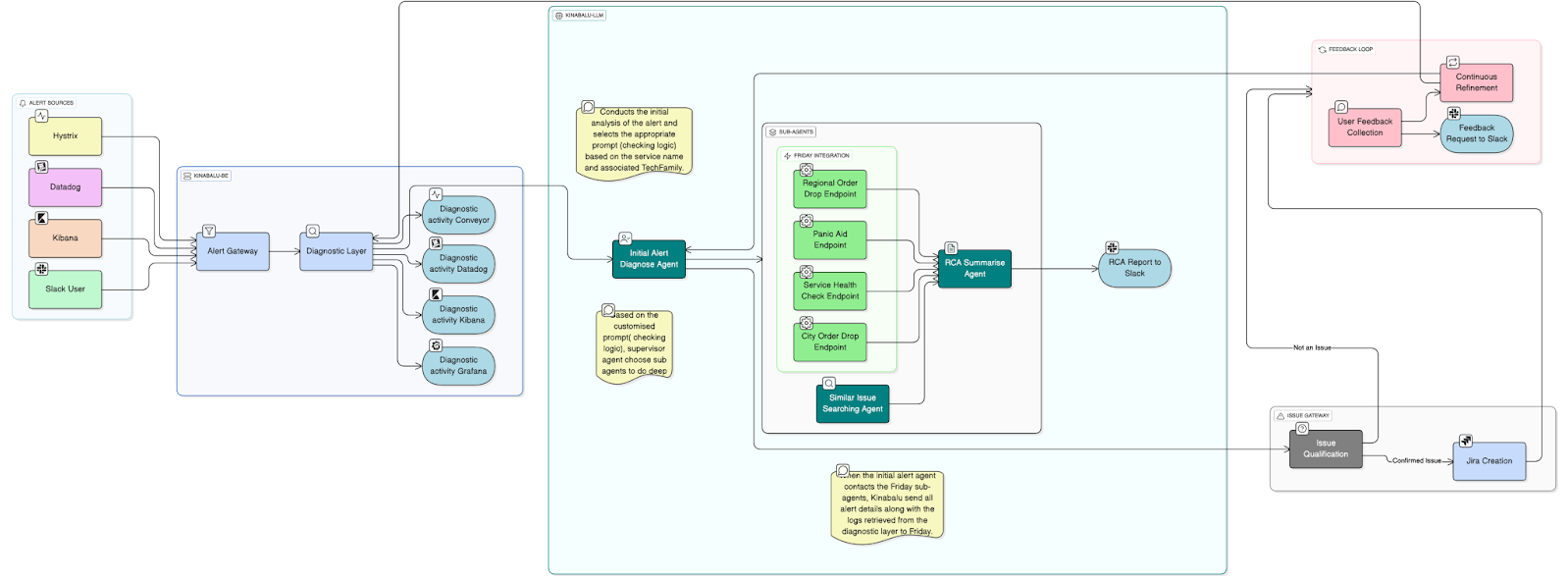
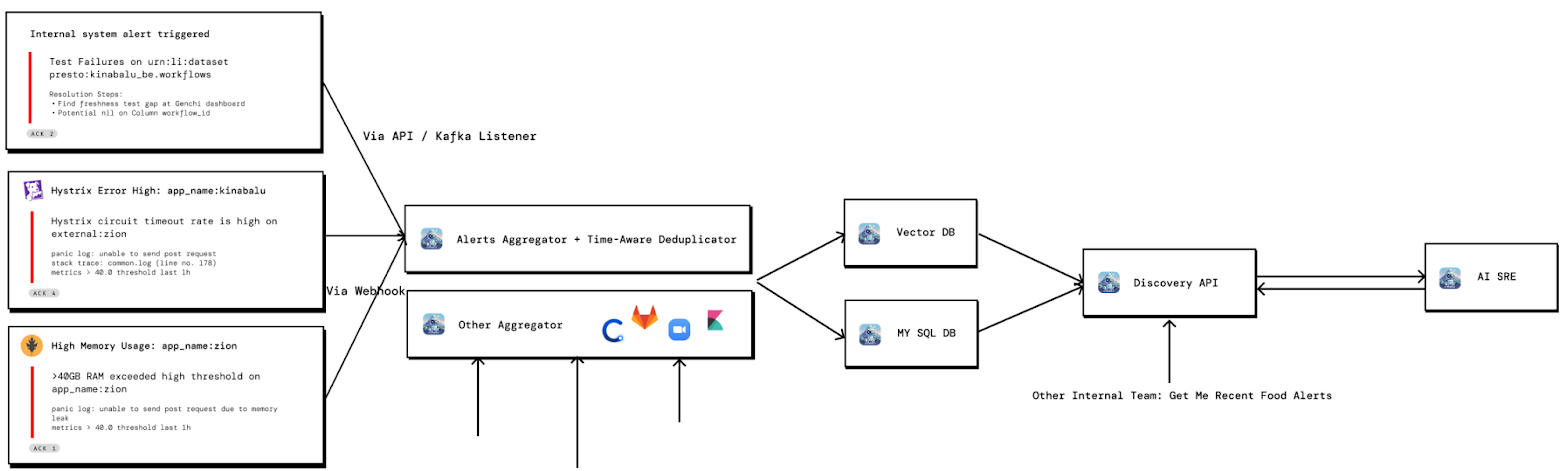
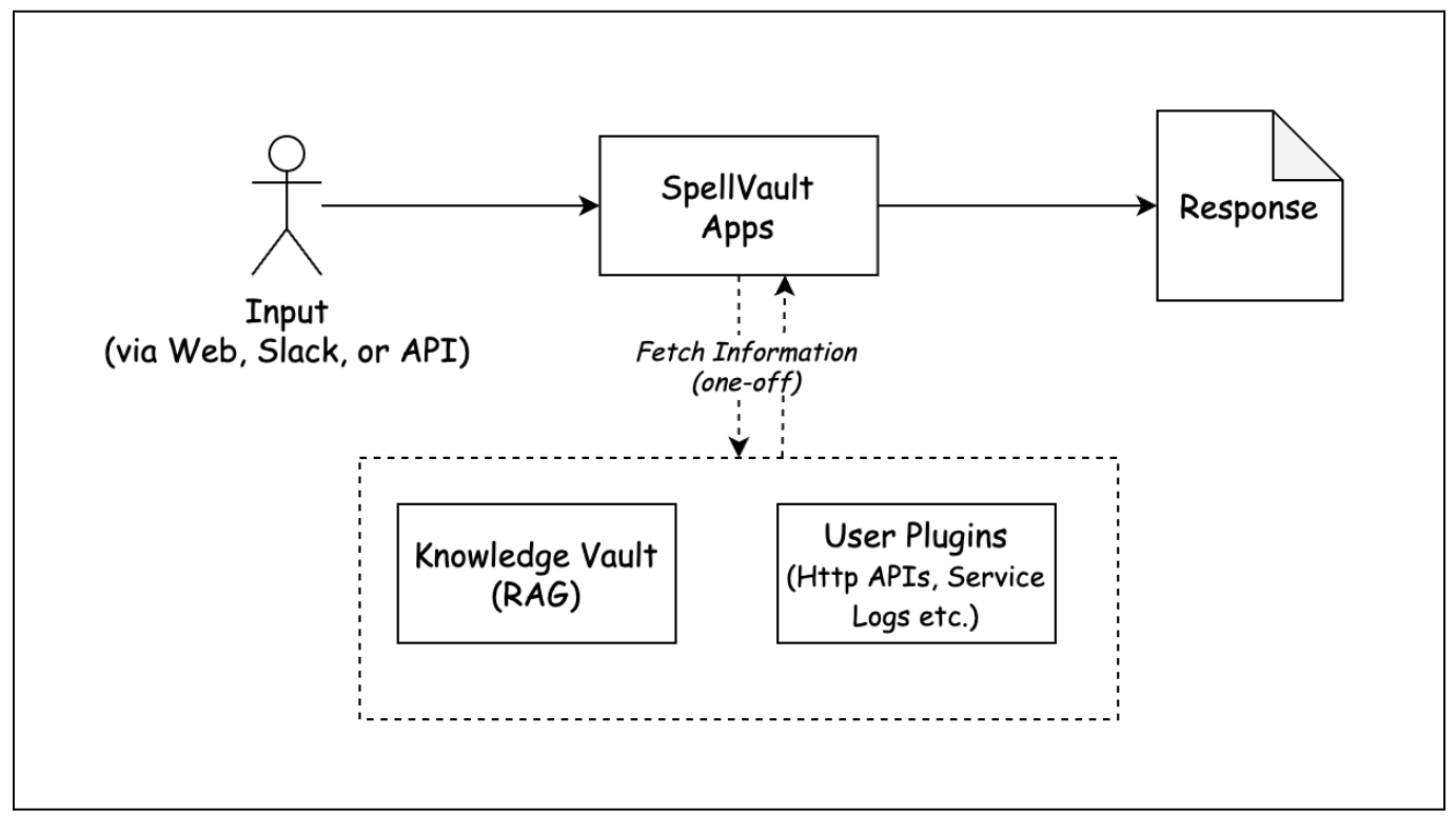
Architecture
Under the hood, the backend combines a central signal aggregator with Model Context Protocol (MCP) servers for instant search, and a Large Language Model (LLM) powered intelligence layer that analyzes signals to auto-triage incidents and produce actionable insights.
Figure 1. SRE AI architecture.
Signal aggregator: Context engineering
We follow a Retrieval Augmented Generation (RAG) approach and are building a knowledge graph that stitches together incident signals across the stack. The aggregator ingests the information as follows:
Datadog (metrics, monitors)
Kibana/Elasticsearch (logs)
Grafana (dashboards)
Hystrix (circuit state)
GitLab/Jira (changes/issues)
CI/CD and deployment metadata
Service/product catalog (ownership, dependencies)
With this context, AI SRE agents can provide a clear view of what changed, when it changed, and who owns it, making incident understanding and debugging faster and more reliable in a near-real-time manner.
Figure 2. Examples of signal aggregation for building context.
Unified intelligence: An agentic approach
Agents can basically “normalize” the alerts and signals, meaning they standardize and interpret them for better understanding. They can semantically search through historical changes that can explain current symptoms, correlate co-occurring signals, and surface likely causes.
AI SRE uses the SuperAgent and A2A multi-agent frameworks to analyze incidents using two workflows, which can coexist.
For static diagnosis, a separate flow collects all data and logs for services via the MCP toolkit and sends them to A2A multi-agents for a deep-dive investigation.
For dynamic analysis, SuperAgent uses the MCP toolkit to investigate and pull real-time data.
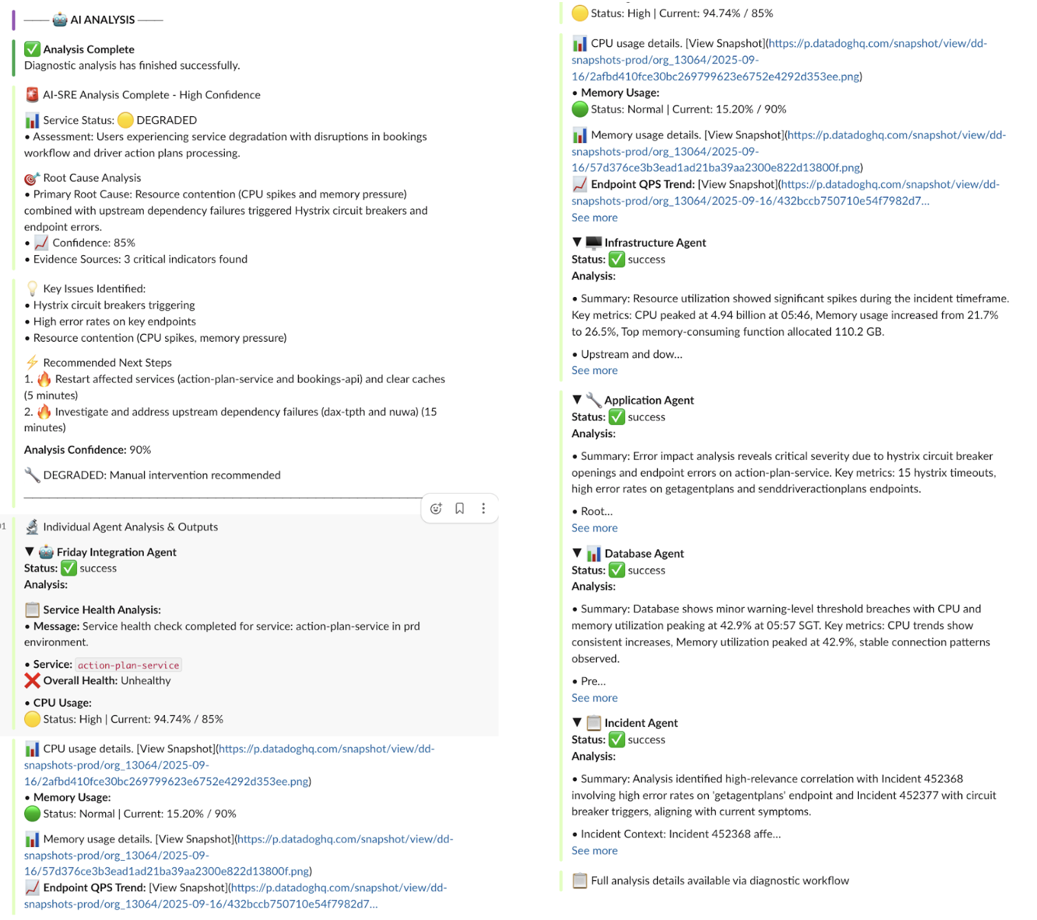
Static diagnosis
The static diagnostics workflow starts with a trigger from Slack or the Web UI and ends with a comprehensive service health report. It coordinates six domain-specific sub-agents encompassing the areas of incident management, deployment, application, database, infrastructure, and external APIs. Each sub-agent pulls the relevant signals and runs targeted checks, producing detailed findings. The supervisor then synthesizes these into an investigation-ready brief. The brief contains a concise summary of suspects and blast radius, timeline, and recommended next steps. The briefs are grounded in logs and metrics, so engineers can quickly understand the impact and move toward resolution.
Figure 3. Examples of static diagnosis by AI SRE.
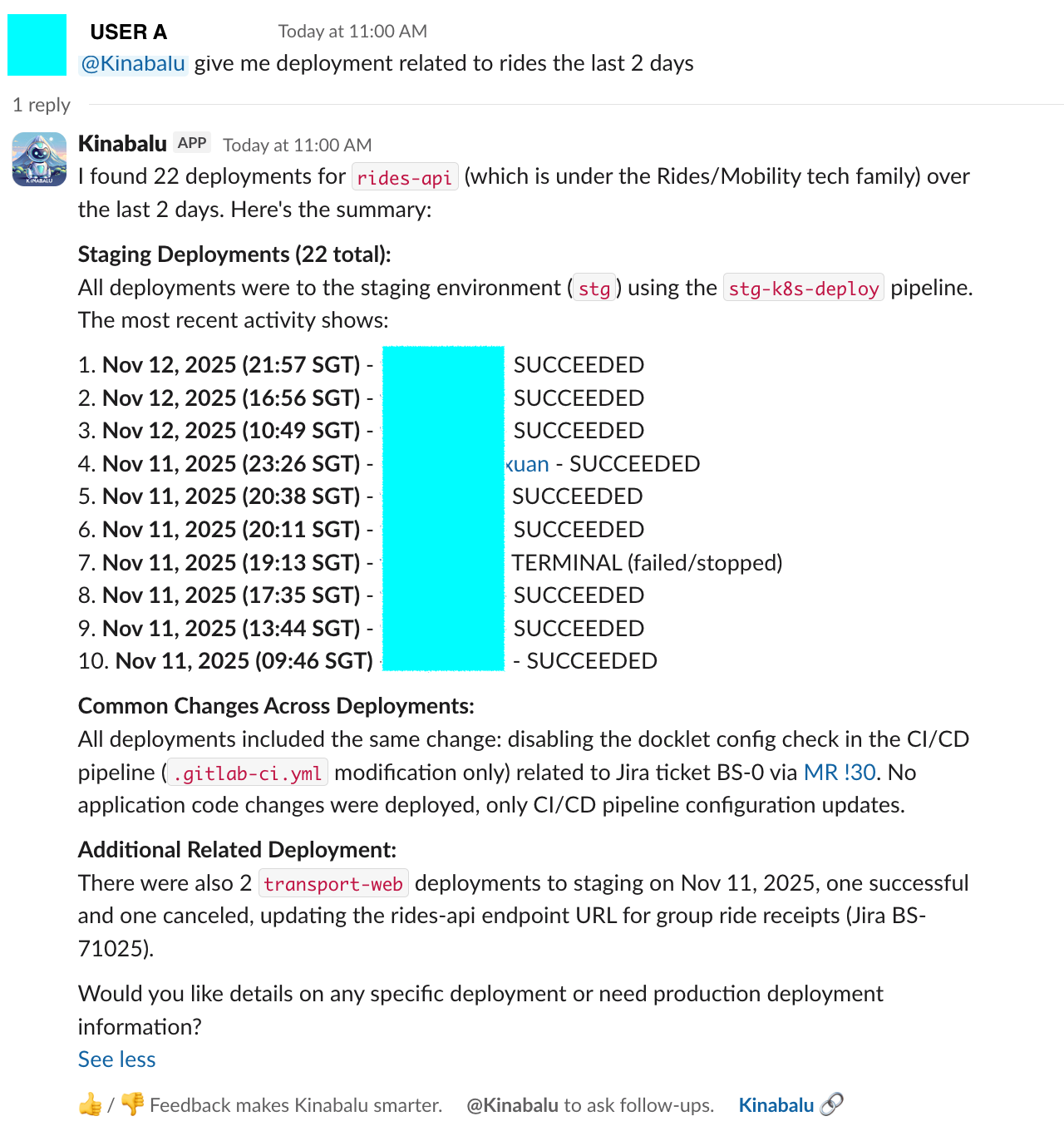
Dynamic chat
Users can inquire via Slack or the Web UI to receive an immediate, evidence-supported action plan. Examples of such questions include:
“How many recent deployments touched the food service?”
“How many Terraform changes in the past 5 minutes?”
Powered by our SuperAgent and MCP tool layer, dynamic chat queries live systems such as metrics, logs, deploy history, and configs. It then returns cited data, comparisons, and next-best actions. On-call engineers can diagnose issues and pull logs on the fly, before escalating actions (e.g., open a ticket, compare regions, list owners, suggest rollbacks). It’s human-in-the-loop (HITL) by design.
Figure 4. Example of examining related deployments within the same time frame.
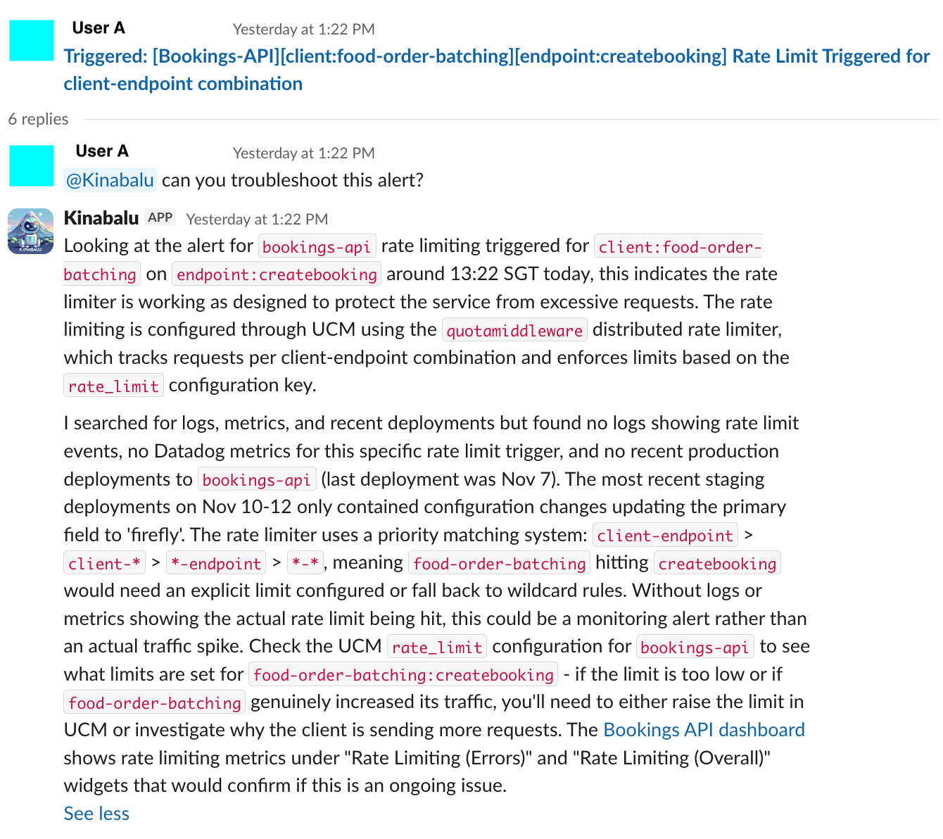
Figure 5. Example of analyzing Splunk or DataDog alerts to identify the root cause of an issue.
MCP toolkit
The Kinabalu MCP Toolkit serves as a universal integration layer that empowers AI SRE by unifying 25 operational tools into a single, consistent interface. This comprehensive toolkit spans six key domains:
Incident and communications: Manages historical incidents, Slack thread context, and ticketing.
Internal platforms: Includes changelogs, experiments, rollout history, and automated analyses.
Knowledge and AI: Facilitates enterprise document search/chat and unstructured data analysis.
Service and configuration: Offers topology and configuration introspection.
Observability: Provides insights through metrics, logs, and profiling.
Deployment: Tracks recent releases and commit history.
The Kinabalu MCP Toolkit is designed to provide AI SRE with a 360 degree view of incidents, significantly accelerating root-cause discovery and response.
Conclusion
Our journey highlights the importance of structured context, robust diagnostic layers, and hybrid AI models for dependable incident automation. With Kinabalu AI SRE, we’re moving toward an ecosystem where alerts are normalized, evidence is automatically synthesized, and engineers can focus on higher level decision-making rather than firefighting.
Stay tuned for part 2, where we will cover the challenges, design decisions, and lessons that shaped Kinabalu AI SRE.
Join us
Grab is a leading superapp in Southeast Asia, operating across the deliveries, mobility and digital financial services sectors. Serving over 800 cities in eight Southeast Asian countries, Grab enables millions of people everyday to order food or groceries, send packages, hail a ride or taxi, pay for online purchases or access services such as lending and insurance, all through a single app. Grab was founded in 2012 with the mission to drive Southeast Asia forward by creating economic empowerment for everyone. Grab strives to serve a triple bottom line – we aim to simultaneously deliver financial performance for our shareholders and have a positive social impact, which includes economic empowerment for millions of people in the region, while mitigating our environmental footprint.
Powered by technology and driven by heart, our mission is to drive Southeast Asia forward by creating economic empowerment for everyone. If this mission speaks to you, join our team today!
Troubleshooting critical issues by deciphering a user’s journey on the Grab app is an extremely challenging task. With countless user journeys and multiple paths through the User Interface (UI), it’s akin to searching for a needle in a vast haystack. This challenge frequently resonates with us, the dedicated developers at Grab, as we strive to understand user behaviors, views, and interactions.
The challenge
The distinction between resolving an issue effectively versus spending hours on a wild goose chase is understanding our user journey in real-time.
The development team initially attempted to address the issue of the incomplete user journey tracking by implementing a system where a click stream event would be sent with every user interaction. However, this approach presented significant challenges due to the sheer volume of UI components—often numbering in the hundreds—and the reliance on individual developers to correctly instrument each one.
A common pitfall was that developers would occasionally overlook or forget to instrument certain user interactions, leading to breaks in the recorded user journey. This created a highly frustrating situation for both the development and product teams, as the integrity of the user journey data was consistently compromised. Despite continuous efforts to patch these bugs and address the omissions, the team found themselves in a perpetual state of reaction, constantly trying to catch up with newly discovered breaches rather than proactively preventing them. This reactive approach consumed valuable resources and hindered the ability to gain a complete and accurate understanding of user behavior.
Diagnosing system failures, application bugs, or poor user experiences in complex applications becomes inefficient without real-time performance metrics and detailed session tracking. When engineering teams rely on outdated or fragmented data, they are forced to piece together issue narratives reactively, long after the issues occur. This significantly delays the Mean Time To Resolution (MTTR). Such a reactive approach leads to increased downtime, higher operational costs, customer dissatisfaction, and a waste of developers’ time, as they spend more time “hunting” for clues rather than deploying solutions or new features.
Our ‘Eureka’ moment: AutoTrack SDK
The pivotal breakthrough that provides our unique advantage was the creation of auto tracking user journeys—our “Eureka” moment. To deliver this, we developed the new Software Development Kit (SDK) called AutoTrack.
AutoTrack is system that comprehensively records application state, UI view state, as well as user interactions – a solution that pieces together a chronicle of the user journey, from launch to interactions, as they navigate through the screens. AutoTrack SDK is built on the three core pillars:
Application state
User interactions
UI screens
Let’s delve deeper into the mechanics of how this operates.
Application state
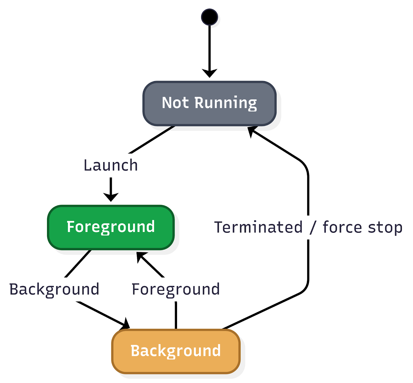
Understanding the application state is fundamental to comprehending user behavior and, consequently, executing effective troubleshooting. The application state provides crucial insights into how a user interacts with the app, particularly concerning its visibility and how it was initiated. This encompasses tracking when the app moves between the background and foreground, as well as the various launch mechanisms.
Figure 1. Application state user flow.
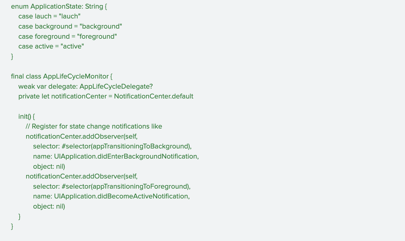
Key aspects of application state that are vital to monitor include: Application lifecycle transitions:
Background state: When the app is running but not actively displayed to the user (e.g., the user switches to another app, or the device is locked). Understanding how frequently and for how long an app resides in the background can inform power consumption analysis and the effectiveness of background tasks.
Foreground state: When the app is actively in use and displayed to the user. Monitoring transitions into and out of the foreground provides a real-time view of user engagement.
Inactive state: A temporary state where the app is in the foreground but not receiving events (e.g., an incoming call temporarily interrupts the app).
Suspended state: An app that is in the background and has been explicitly suspended by the operating system to free up resources.
Terminated state: When the app has been completely closed or crashed. Differentiating between intentional termination and crashes is critical for identifying stability issues.
Application launch mechanisms:
The way an app is launched significantly impacts the initial user experience and can influence subsequent interactions. Tracking these different launch types is essential for understanding user entry points and for debugging issues that might be specific to a particular launch method.
Explicit user launch: This is the most straightforward launch mechanism, where the user directly taps on the app icon from their device’s home screen or app drawer. This indicates a deliberate intent to use the app and often signifies a primary entry point for regular users.
Deeplinks: Deeplinks are URLs that, when clicked, open a specific page or section within a mobile app rather than a web page. They are powerful tools for enhancing user experience and engagement by providing direct access to relevant content.
Push notifications: Push notifications are messages sent by an app to a user’s device even when the app is not actively in use. Tapping on a push notification often launches the app and directs the user to a specific context related to the notification’s content.
Figure 2. Code sample for tracking application lifecycle transition.
User interactions
Real-time session tracking is a crucial component in understanding user behavior and optimizing app performance. By meticulously tracking a wide array of user interactions, the system provides invaluable insights into how users navigate and engage with the app. This granular data forms the bedrock for constructing comprehensive user journeys, allowing development teams to visualise the path a user takes from their initial entry point to achieving their goals within the app.
This deep understanding of user interactions is the most important pillar in creating accurate and insightful user journey maps. These maps, in turn, are instrumental in identifying patterns of user behavior, both positive and negative. For instance, tracking helps to identify pain points, bugs, or areas of confusion that might lead to user frustration or abandonment.
Figure 3. Sample code for real-time session tracking.
UI screen
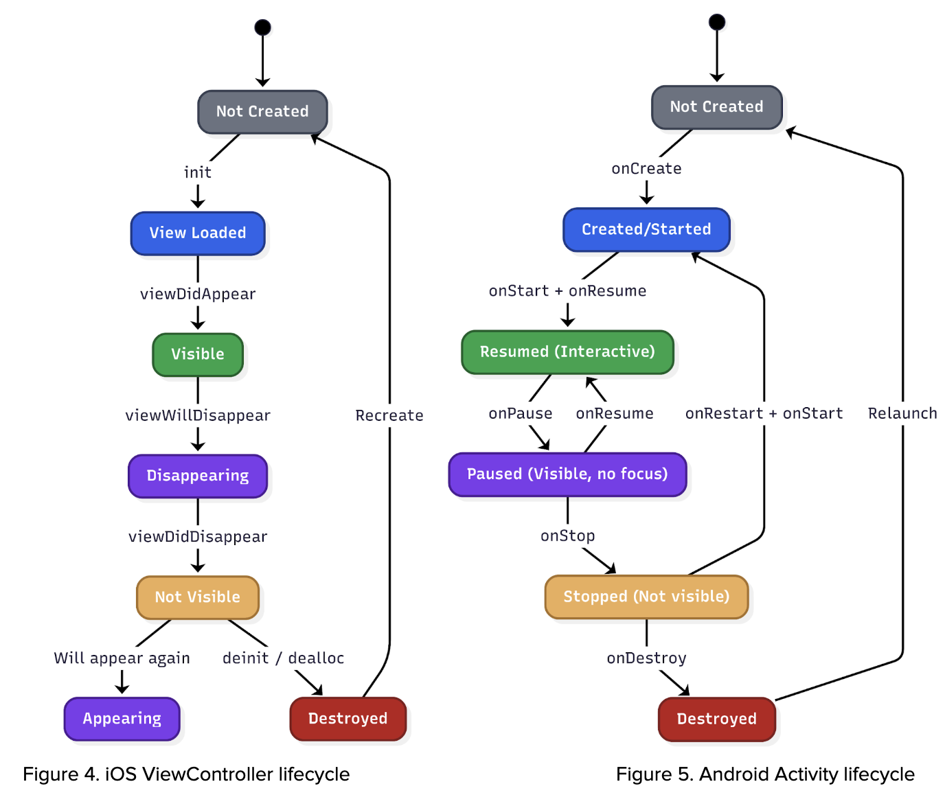
The system leverages lifecycle events from UIViewController (iOS), Activity (Android), and Fragments (Android) to accurately identify and track which specific screen is currently displayed to the user. This granular level of screen tracking is crucial because it significantly enriches the contextual information available to us. By understanding the precise UI that users are interacting with, we can account for the dynamic nature of our app. Different geographical regions, diverse user segments, and varying operational scenarios can lead to distinct user interfaces being presented. This capability ensures that our analysis and troubleshooting efforts are always based on the actual user experience, allowing for more precise problem identification and more effective solutions.
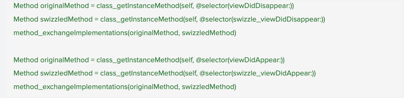
Figure 6. Sample code of UIViewController configuration.
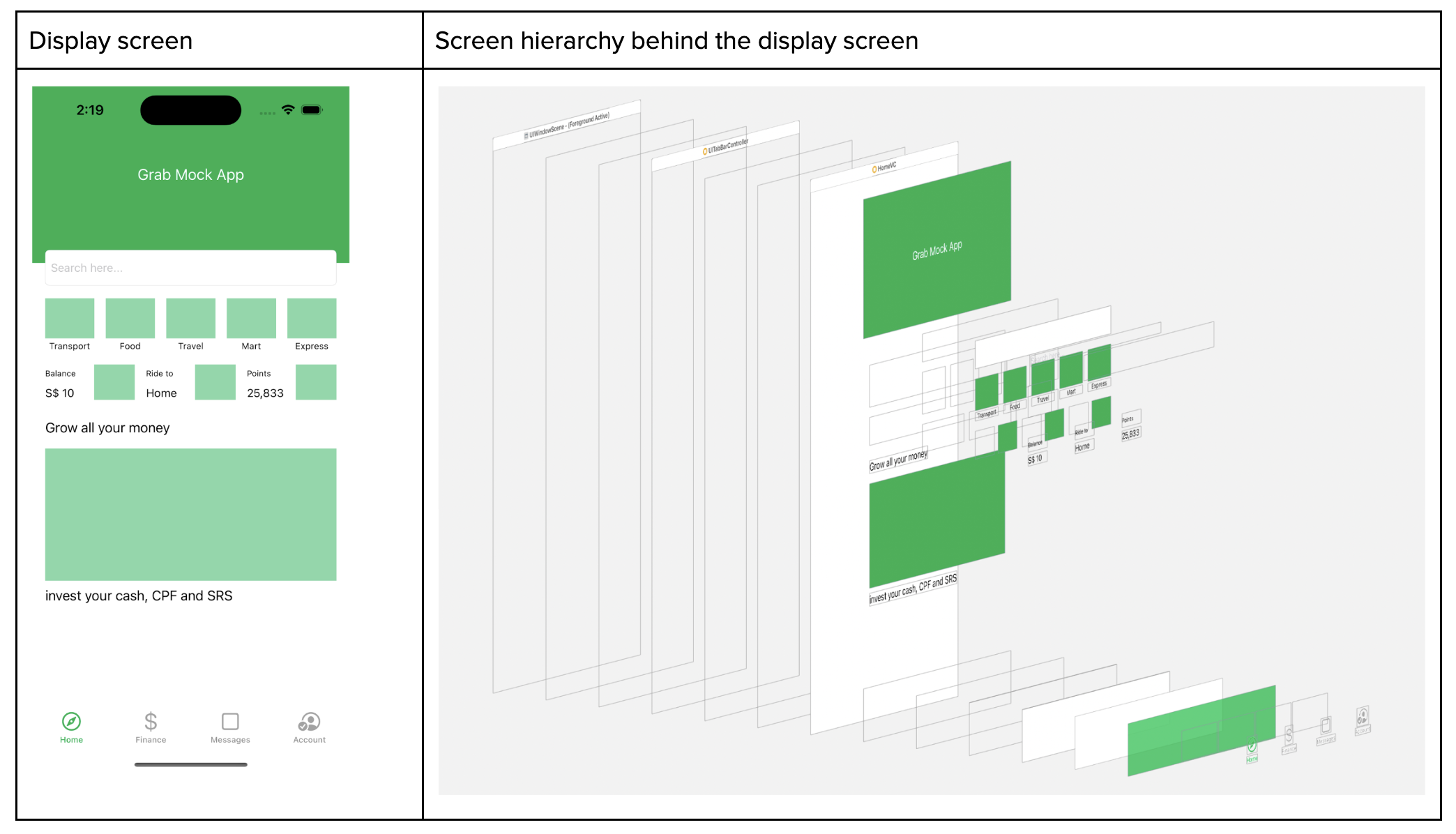
UI screen data
On top of that, whenever the screen appears, we capture the screen metadata where we read the full screen hierarchy. With the Screen hierarchy JSON data at hand, we employ it to train an AI model. This model, consequently, can generate an HTML file, which mirrors the user’s screen and interaction.
Disclaimer: information is redacted in compliance with GDPR/PDPA, personal data protection laws.
Figure 7. Screen hierarchy.
Applications of AutoTrack
Key applications of AutoTrack data:
Reconstructing user journeys and reproducing elusive bugs: One of the most significant benefits of AutoTrack is its ability to meticulously record user interactions within the app. This detailed session data allows our teams to precisely recreate the user journey that led to a reported issue. For bugs that are notoriously difficult to reproduce, this capability is a game-changer, eliminating hours of manual guesswork and dramatically accelerating the identification and resolution of underlying problems.
Automated issue assignment: When an issue is reported, AutoTrack data can be leveraged to automatically assign it to the most relevant team. By analysing the context of the issue within the recorded session, including the specific features or modules involved, the system can intelligently route the problem to the engineers best equipped to address it. This automation reduces triage time, ensures issues are handled by subject matter experts, and improves overall response efficiency.
Automating UI test case generation: The rich dataset provided by AutoTrack offers a powerful foundation for automating the creation of UI test cases. By observing how users interact with the interface, we can automatically generate test scripts that mimic real-world usage patterns. This not only speeds up the testing phase but also leads to more comprehensive test coverage, identifying edge cases and user flows that might otherwise be missed by manually written tests.
Understanding analytics event triggers: AutoTrack data provides a granular view into when and why specific analytics events are triggered within the application. This allows us to validate the accuracy of our analytics instrumentation, ensure that events are firing as expected, and gain deeper insights into user behavior. By understanding the precise context surrounding event triggers, we can refine our data collection strategies and derive more meaningful insights from our analytics.
Key takeaways and what’s next
AutoTrack replaces fragile manual instrumentation with a unified, real-time view of application state, screen context, and user interactions. That end-to-end trace makes elusive bugs reproducible, routes issues to the right owners, and seeds reliable UI tests—turning guesswork into grounded evidence so teams can ship fixes faster and with greater confidence.
Looking ahead, we are expanding AutoTrack across surfaces and deepening the context it captures—pairing sessions with network and performance signals, strengthening privacy guardrails, and integrating with automated triage and test generation. Look forward to reading more of our deep dives on auto-generated UI tests and how these journeys will power proactive quality across Grab’s app.
Join us
Grab is a leading superapp in Southeast Asia, operating across the deliveries, mobility and digital financial services sectors. Serving over 800 cities in eight Southeast Asian countries, Grab enables millions of people everyday to order food or groceries, send packages, hail a ride or taxi, pay for online purchases or access services such as lending and insurance, all through a single app. Grab was founded in 2012 with the mission to drive Southeast Asia forward by creating economic empowerment for everyone. Grab strives to serve a triple bottom line – we aim to simultaneously deliver financial performance for our shareholders and have a positive social impact, which includes economic empowerment for millions of people in the region, while mitigating our environmental footprint.
Powered by technology and driven by heart, our mission is to drive Southeast Asia forward by creating economic empowerment for everyone. If this mission speaks to you, join our team today!
Delivering personalized user experiences in real-time is central to Grab’s strategy, but achieving this at scale poses significant engineering challenges. Grab’s Customer Data Platform (CDP) and Growth team has successfully delivered several real-time campaigns, driving significant business impact through enhanced personalization. These initiatives include high-impact use cases like immediate mall offers, timely traveler recommendations, precise ad retargeting, and proactive interventions during key user journey moments. At the core of these successes is Grab’s CDP, which rapidly deploys advanced real-time personalization via a powerful new capability called “Scenarios.”
About Grab’s CDP
Grab’s CDP is a centralized, reliable repository for user attributes, designed for freshness, governance, and reusability. Built on Grab’s Signal Marketplace framework, the CDP streamlines data management through automation and integration, supporting seamless interactions with internal services and toolings that power marketing, experimentation, ads, Machine Learning (ML) features, and external platforms, including Facebook, Google Ads, and TikTok.
The platform currently manages over 1,000 batch user attributes for Passengers, Drivers, and Merchants, powering diverse use cases from targeted marketing campaigns to operational decision-making across Grab’s entire ecosystem.
The need for real-time personalization
In our current CDP setup, user segments are primarily created for targeting using batch attributes that update once daily. While these batch updates provide valuable historical insights, they are not suitable for scenarios requiring real-time responsiveness. This delay prevents timely engagement with users, particularly when immediate actions can significantly enhance user experiences and conversion rates.
For example, when travelers land at an airport, they immediately benefit from timely suggestions for rides, dining options, or local attractions. Traditional batch processing cannot deliver the agility and responsiveness required for these dynamic scenarios.
Historically, real-time personalization at Grab relied heavily on engineering resources, which resulted in limited scalability and agility. Marketers and product teams often found themselves blocked by engineering bandwidth constraints, restricting experimentation and innovation.
Problem statement
The limitations of Grab’s existing personalization frameworks include:
Batch attribute delays: Daily updates are insufficient for scenarios requiring immediate user responses.
Limited dynamic enrichment: Difficulties in dynamically integrating real-time events with historical user data, weakens personalization effectiveness.
High engineering overhead: Custom solutions require extensive resources, limiting agility and innovation.
To overcome these challenges and support Grab’s vision for comprehensive personalization – including proactive recommendations and assistance – CDP needed robust real-time capabilities.
CDP Scenarios: Real-time personalization made simple
The Scenario feature revolutionizes real-time targeting within the CDP by utilizing user-initiated events, geo-fencing, historical profile data, and on-the-fly predictions. This empowers the business to deliver easy, quick, and flexible personalization without the need for complex engineering efforts.
Scenarios enable innovative use cases such as these:
Mall personalization: Real-time personalized offers upon arrival.
Traveler assistance: Immediate recommendations at airports or hotels.
Ad retargeting: Enhanced real-time ad targeting.
Conversion optimization: Timely intervention during user drop-off points.
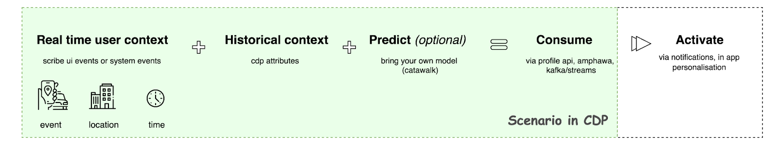
Imagine predicting a user’s intent to drop off at a mall using both real-time and historical context. For instance, when a user books a ride to a mall, factors such as destination, time, cuisine preferences, and past behavior (e.g., affluence level) can help predict whether the user’s purpose is retail therapy, grocery shopping, or dining out. This prediction accounts for elements like time of day, day of the week, and mall location. Grab’s engineering teams can leverage this predicted intent (signal) to offer personalized actions, such as GrabPay discounts for shopping or exclusive dining offers for dinner.
Figure 1. Scenario in CDP.
Key features
Event-driven personalization: Real-time Scenarios triggered by Scribe events (Grab’s comprehensive event collection and tracking platform) combined with geo-fencing.
Historical context integration: Optionally enrich Scenarios using historical CDP data.
Predictive modeling: Deploy pre-trained models for instant user behavior predictions.
Self-serve graphical user interface (GUI): Enable marketers to create complex event sequences and validate Scenarios with synthetic data processed through Flink pipelines.
Headless application programming interfaces (APIs): Allow programmatic access and management of Scenarios.
Figure 2. Attributes for a scenario in CDP.
Self-serve Scenario creation
We designed an intuitive self-serve UI, embedded within the Grab app, empowering marketers to quickly define and deploy Scenarios. Users can specify event triggers, configure geo-fencing, incorporate historical user attributes, and select predictive models. Marketers can also validate Scenarios using synthetic data before deployment, ensuring accurate and realistic outcomes.
How it works:
Select event triggers: Choose predefined events or define custom intra-session sequences via the GUI.
Configure geo-fencing: Define Scenario activation locations, like airports or malls.
Include historical attributes (optional): Utilize batch attributes from the CDP to enrich Scenarios.
Select predictive models (optional): Train custom classifiers or pick from pre-trained Catwalk models.
Define data sink: Choose between Amphawa (DynamoDB), Kafka, or both; potentially extendable to external destinations (e.g., Appsflyer).
Once configured, metadata synchronizes automatically with our streaming service, and Scenarios become available for real-time consumption within an hour.
Proven impact: Real-world success
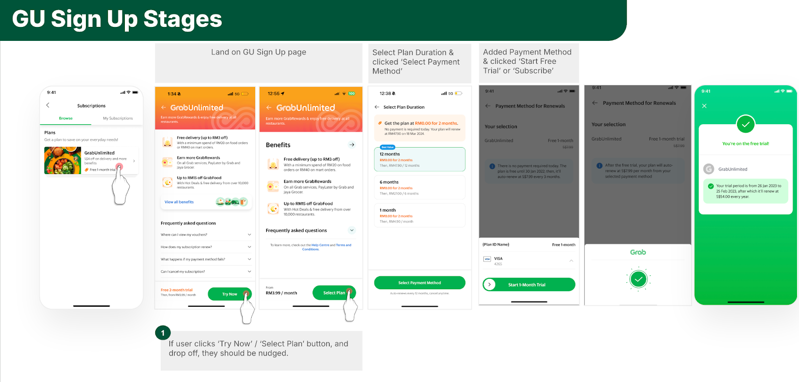
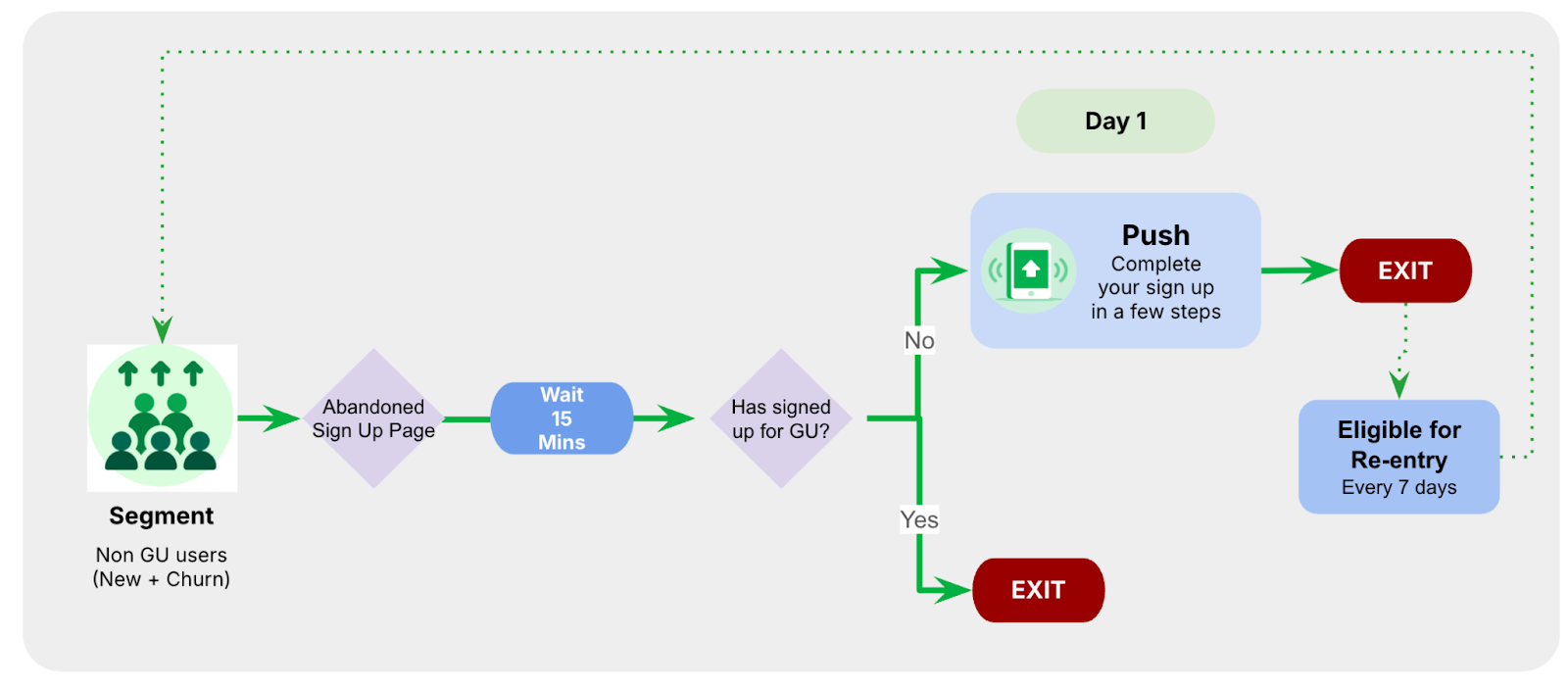
CDP Scenarios are already delivering measurable business results, with over 12 live production implementations. For instance, in a case study addressing Grab Unlimited subscription signup abandonment, we leveraged CDP Scenarios to increase signups by engaging users in real time within 15 minutes of them leaving the signup process.
Figure 3. Grab Unlimited sign-up journey.
To enhance conversion rates, personalized real-time nudges were deployed through Scenarios. For example, users who started the signup process but failed to complete it within 15 minutes received a follow-up notification, prompting them to finalize their registration.
Figure 4. Scenario flow for Grab Unlimited registration.
This scenario alone achieved more than a 3% uplift in subscriber conversions vs non-real-time acquisition campaigns, demonstrating Scenarios’ potential to significantly boost business outcomes.
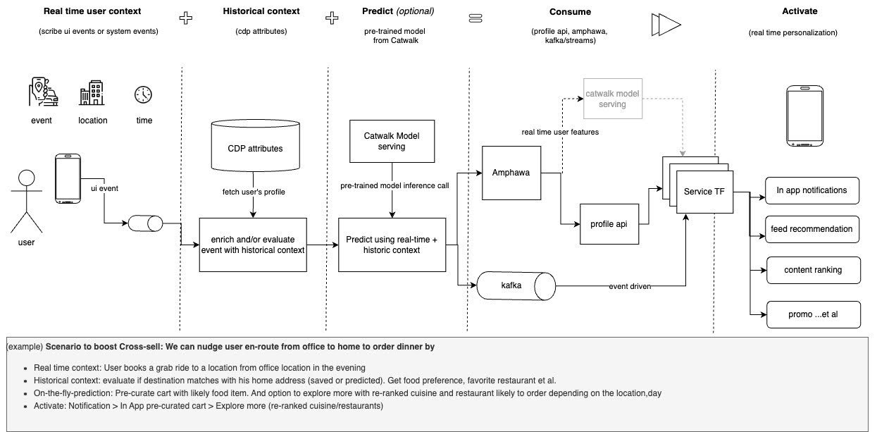
Technical architecture: Low latency, high reliability
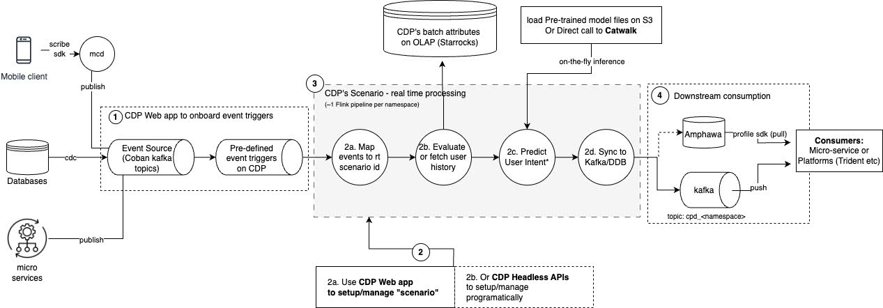
Figure 5. High-level scenario flow. Scenarios are designed for low latency (under 15 seconds) and high reliability.
Event registration: Popular UI events from Scribe are whitelisted and immediately available; custom events are onboarded via the CDP web portal.
Scenario creation: Users configure Scenarios through a user-friendly GUI, defining events, historical contexts, and predictive models.
Real-time Flink processing: Incoming events trigger Scenarios, evaluating user historical data via StarRocks and performing real-time predictions using pre-trained models.
Real-time data sync: Outcomes are synced back to Kafka or Amphawa (Grab’s internal feature store built on AWS DynamoDB), enriching data for use by subsequent services.
Consumption by downstream services: Kafka streams or CDP’s Profile SDK facilitates immediate, personalized user experiences.
Advancing the future of real-time personalization
As we continue to innovate, we are focused on enhancing the capabilities of CDP Scenarios to support more complex and scalable personalization use cases. Here are some key areas of improvement we are exploring:
Optimized Scenario sharding for scalable processing: To accommodate the growing number of use cases, we plan to scale and orchestrate our Flink pipeline fleet in a headless manner. This approach will improve system stability and enable seamless management of complex Scenarios across the pipeline.
Enhanced signal distribution across multiple destinations: Currently, Scenario outputs are limited to a single topic or sink. To address the increasing diversity of use cases, we aim to expand signal distribution, allowing downstream consumers to access Scenario outcomes through multiple scalable and reliable channels.
Advanced scheduling and delayed triggering: While real-time computation of Scenario signals is effective, certain use cases require delayed activation for maximum impact. We are exploring ways to compute signals instantly but trigger actions at scheduled times, such as sending a push notification for booking a return Grab ride based on the average wait time at the drop-off location.
The launch of CDP Scenarios represents a significant milestone for Grab, paving the way for scalable, efficient, and user-friendly real-time personalization. Initial successes have demonstrated its immense potential, delivering notable improvements in user engagement and conversion rates. Looking ahead, we are committed to continuously advancing Scenarios by expanding its features, integrations, and applications to further elevate user experiences across the Grab ecosystem.
Join us
Grab is a leading superapp in Southeast Asia, operating across the deliveries, mobility and digital financial services sectors. Serving over 800 cities in eight Southeast Asian countries, Grab enables millions of people everyday to order food or groceries, send packages, hail a ride or taxi, pay for online purchases or access services such as lending and insurance, all through a single app. Grab was founded in 2012 with the mission to drive Southeast Asia forward by creating economic empowerment for everyone. Grab strives to serve a triple bottom line – we aim to simultaneously deliver financial performance for our shareholders and have a positive social impact, which includes economic empowerment for millions of people in the region, while mitigating our environmental footprint.
Powered by technology and driven by heart, our mission is to drive Southeast Asia forward by creating economic empowerment for everyone. If this mission speaks to you, join our team today!
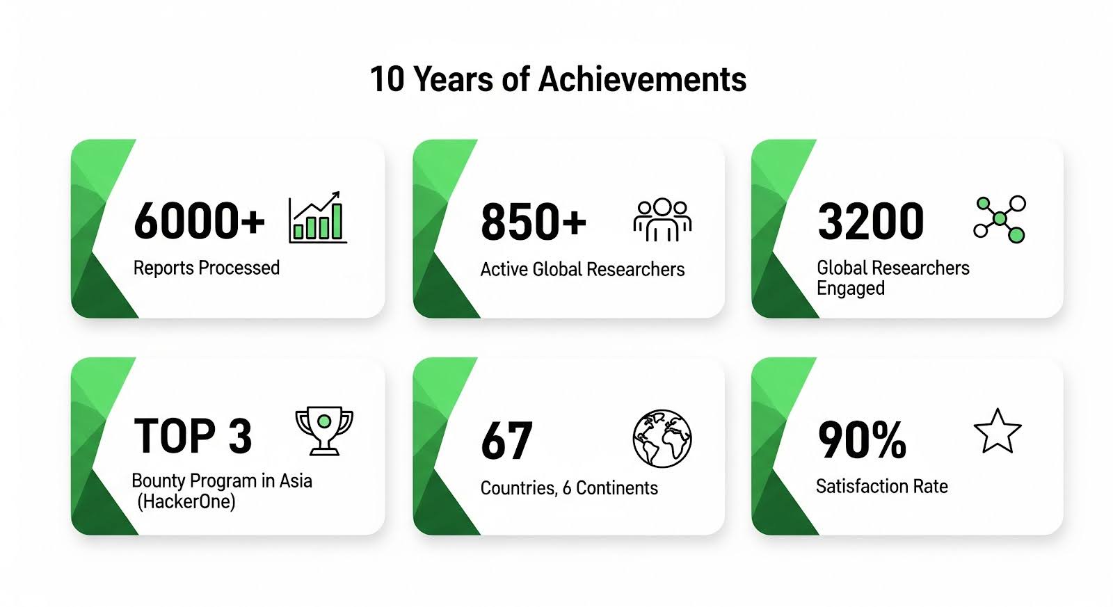
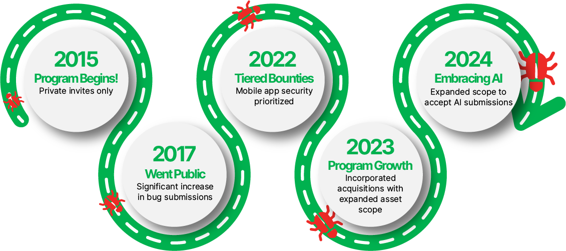
Ten years ago, we launched our bug bounty program in partnership with HackerOne. Beyond a security initiative, it represented an open invitation to collaborative development.
As pioneers in Southeast Asia, we began the program with 23 initial researchers, and it has since evolved into a global community of security researchers.
The strategic structure and scope of our Bug Bounty Program, combined with our continuous innovation and experimentation, have successfully captured the attention of the global security research community. Over the past decade, we have partnered with more than 850 active security researchers from HackerOne’s community of over 2 million cybersecurity professionals worldwide. These dedicated researchers work alongside us across borders and time zones, forming a collaborative defense network that helps protect over 187 million users throughout Southeast Asia. Their ongoing participation demonstrates both the maturity of our program and the trust we’ve built within the security research community.
This milestone reflects the strength of shared purpose and our sustained partnership with the HackerOne platform. It demonstrates the value of human connection and the collective understanding that security is stronger through collaboration. Here’s to a decade of partnership and to many more years of building a safer future, one collaboration at a time!
Figure 1. Ten years of achievements with our HackerOne partnership.
Evolution and growth: Adapting to a dynamic threat landscape
Over the past ten years, our program has consistently adapted to the dynamic threat landscape and integrated invaluable feedback from our research community. We have grown from a private initiative to a program that consistently ranks among the top 20 worldwide and among the top 3 in Asia on HackerOne. Key milestones from our journey include:
Expanding our horizons: Our scope significantly broadened in 2023-2024, continuously adding new assets and prominently including financial services in Indonesia and AI systems. This expansion provides researchers with more avenues to contribute to Grab’s security.
Focused mobile security: We introduced a dedicated bounty table for mobile-specific issues, recognizing the unique challenges of mobile security.
Incentivizing excellence: We regularly experiment with campaigns of various types and targets, diversifying our reward methods to include both financial rewards and recognition.
Evolving vulnerability focus: We’ve observed a significant shift in the types of vulnerabilities reported over the decade, moving from foundational issues in early years to more sophisticated and emerging categories recently.
Figure 2. The journey of our bug bounty program.
The global stage: Connecting with the best
Our program’s success is deeply rooted in its vibrant global community, which we actively foster through continuous engagement. Our strategy extends beyond the platform to major live hacking events, including the ThreatCon Live Hacking Event 2023in Nepal and DEFCON 32’s Live Recon Village 2024 in Las Vegas. These initiatives have been instrumental in connecting us with a diverse pool of new talent and strengthening relationships with researchers across different continents. By meeting hackers where they are, we’ve not only brought new expertise into our ecosystem but also demonstrated our commitment to being an accessible and collaborative partner on a global scale.
The high participation and quality submissions from these events demonstrate the effectiveness of this approach. They’ve expanded our global security testing coverage and strengthened our standing within the worldwide cybersecurity community. Through ongoing interactions and submitted reports, we continue to see that security is a collaborative effort with no borders.
Exclusive anniversary celebrations: Global club campaigns
To commemorate our 10th anniversary, we launched three exclusive, invite-only campaigns with HackerOne’s regional clubs in Germany, Morocco, and India. These campaigns served as cultural exchanges, bringing fresh perspectives from outside our core Southeast Asian consumer markets. By engaging with these clubs, we expanded our researcher community and connected with security experts who understand different threat landscapes and methodologies, bringing outside perspectives to our systems.
In August, we also ran a broader anniversary campaign that drew significant participation from the researcher community, resulting in 461 submissions. xchopath was awarded the Best Hacker Bonus for their contributions during this campaign.
These campaigns expanded our global security testing coverage and strengthened relationships with international researcher communities. Beyond vulnerability reports, they functioned as knowledge-sharing initiatives. We connected directly with researchers to learn from their experience and feedback, creating a continuous loop of improvement. This international collaboration also informed our global expansion security strategy by providing insights into how different regions approach digital payments and authentication.
The anniversary campaigns allowed us to validate our security frameworks against diverse regulatory environments and advanced testing methodologies from established security markets, reinforcing our commitment to maintaining robust security standards.
Voices from our community
Behind every vulnerability report is a researcher who chose to help make Grab safer. Their perspectives reveal the human side of our security evolution. These individuals are not just cybersecurity experts; they are partners in our mission to protect millions of users and ensure a safe digital environment. Here are a few testimonies from participants in our past campaigns:
“The triage was very fast despite the time difference, which I really appreciated. The triaging experience was better than other programs. The huge scope and business portal with different user roles made it especially interesting to explore.” – ArtSec[H1 Germany club campaign participant]
“I liked that different countries have different features—this gives me more attack surface to explore. Response time was great, triage was very fast, and I appreciated Grab’s effort in providing fast responses. The scope was huge with a lot of wildcards for reconnaissance.” – Sicksec[H1 Morocco club campaign participant]
“More than 20 bugs were reported, and was particularly happy that bounties were being paid upon triage. The Germany team spent a lot of time on the educational part, especially for newcomers. Communication overall was very good, and the immediate response even outside working hours was really cool. SSO and authentication is my expertise and I liked that aspect of exploring the platform.” – Lauritz[H1 Germany club campaign participant]
The road ahead: Our commitment to a secure future
With a strong community of security researchers across countries and a decade of collaboration, we’ve built meaningful partnerships. Every vulnerability report represents trust, and every discovery reflects dedication to our shared mission. The program demonstrates our choice to build together rather than work in isolation, to protect rather than exploit, and to collaborate rather than compete.
While we celebrate our external community, the success of our program relies equally on our dedicated internal teams. Our cybersecurity teams form the operational foundation of this initiative. Their consistent responsiveness and researcher-focused approach have enabled vulnerability reporting to evolve into a genuine partnership, maintaining researcher trust and keeping Grab secure.
The next ten years will bring challenges we can’t yet imagine, from emerging threats in artificial intelligence to novel cryptographic approaches in a quantum-powered world. We will face them together as a community that spans cultures, time zones, and expertise.
Together, we’ll continue securing Southeast Asia’s digital future, one partnership, one discovery, one shared achievement at a time.
Join us
Grab is a leading superapp in Southeast Asia, operating across the deliveries, mobility, and digital financial services sectors. Serving over 800 cities in eight Southeast Asian countries, Grab enables millions of people every day to order food or groceries, send packages, hail a ride or taxi, pay for online purchases or access services such as lending and insurance, all through a single app. Grab was founded in 2012 with the mission to drive Southeast Asia forward by creating economic empowerment for everyone. Grab strives to serve a triple bottom line – we aim to simultaneously deliver financial performance for our shareholders and have a positive social impact, which includes economic empowerment for millions of people in the region, while mitigating our environmental footprint.
Powered by technology and driven by heart, our mission is to drive Southeast Asia forward by creating economic empowerment for everyone. If this mission speaks to you, join our team today!
In today’s data-driven landscape, monitoring data quality has become a critical need for ensuring reliable and efficient data usage across domains. High-quality data is the backbone of AI innovation, driving efficiency and unlocking new opportunities. As decentralized data ownership grows, the ability to effectively monitor data quality is essential for maintaining reliability in data systems.
Kafka streams, as a vital component of real-time data processing, play a significant role in this ecosystem. However, unreliable data within Kafka streams can lead to errors and inefficiencies for downstream users, and monitoring the quality of data within these streams has always been a challenge. This blog introduces a solution that empowers stream users to define a data contract, specifying the rules that Kafka stream data must adhere to. By leveraging this user-defined data contract, the solution performs automated real-time data quality checks, identifies problematic data as it occurs, and promptly notifies stream owners. This ensures timely action, enabling effective monitoring and management of Kafka stream data quality while supporting the broader goals of data mesh and AI-driven innovation.
Problem statement
In the past, monitoring Kafka stream data processing lacked an effective solution for data quality validation. This limitation made it challenging to identify bad data, notify users in a timely manner, and prevent the cascading impact on downstream users from further escalating.
Challenges in syntactic and semantic issue identification:
Syntactic issues: Refers to schema mismatches between producers and consumers, which can lead to deserialization errors. While schema backward compatibility can be validated upon schema evolution, there are scenarios where the actual data in the Kafka topic does not align with the defined schema. For example, this can occur when a rogue Kafka producer is not using the expected schema for a given Kafka topic. Identifying the specific fields causing these syntactic issues is a typical challenge.
Semantic issues: Refers to inconsistencies or misalignments between producers and consumers about the expected pattern or significance of each field. Unlike Kafka stream schemas, which act as a data structure contract between producers and consumers, there is no existing framework for stakeholders to define and enforce field-level semantic rules, for example, the expected length or pattern of an identifier.
Timeliness challenge in data quality monitoring: There is no real-time mechanism to automatically validate data against predefined rules, timely identify quality issues, and promptly alert stream stakeholders. Without real-time stream validation, data quality issues can sometimes persist for periods of time, impacting various online and offline downstream systems before being discovered.
Observability challenge for troubleshooting bad data: Even when problematic data is identified, stream users face difficulties in pinpointing the exact “poison data” and understanding which fields are incompatible with the schema or violate semantic rules. This lack of visibility complicates Root Cause Analysis and resolution efforts.
Solution
Our Coban platform offers a standardized data quality test and observability solution at the platform level, consisting of the following components:
Data Contract Definition: Enables Kafka stream stakeholders to define contracts that include schema agreements, semantic rules that Kafka topic data must comply with, and Kafka stream ownership details for alerting and notifications.
Automated Test Execution: Provides a long running Test Runner to automatically execute real-time tests based on the defined contract.
Real-time Data Quality Issue Identification: Detects data issues at both syntactic and semantic levels in real-time.
Alerts and Result Observability: Alerts users, simplifying observation of data quality issues via the platform.
Architecture details
The solution includes three components: Data Contract Definition, Test Execution & Data Quality Issue Identification, and Result Observability as shown in the architecture diagram in figure 1. All mentions of “Flow” from here onwards refer to the corresponding processes illustrated in figure 1.
Figure 1. Real-time Kafka Stream Data Quality Monitoring Architecture diagram.
Data Contract Definition
The Coban Platform streamlines the process of defining Kafka stream data contracts, serving as a formal agreement among Kafka stream stakeholders. This includes the following components:
Kafka Stream Schema: Represents the schema used by the Kafka topic under test and helps the Test Runner to validate schema compatibility across data streams (Flow 1.1).
Kafka Stream Configuration: Encompasses essential configurations such as the endpoint and topic name, which the platform automatically populates (Flow 1.2).
Observability Metadata: Provides contact information for notifying Kafka stream stakeholders about data quality issues and includes alert configurations for monitoring (Flow 1.3).
Kafka Stream Semantic Test Rules: Empowers users to define intuitive semantic test rules at the field level. These rules include checks for string patterns, number ranges, constant values, etc. (Flow 1.5).
LLM-Based Semantic Test Rules Recommendation: Defining dozens if not hundreds of field-specific test rules can overwhelm users. To simplify this process, the Coban Platform uses LLM-based recommendations to predict semantic test rules using provided Kafka stream schemas and anonymized sample data (Flow 1.4). This feature helps users set up semantic rules efficiently, as demonstrated in the sample UI in figure 2.
Figure 2. Sample UI showcasing LLM-based Kafka stream schema field-level semantic test rules. Note that the data shown is entirely fictional.
Data Contract Transformation
Once defined, the Coban Platform’s transformation engine converts the data contract into configurations that the Test Runner can interpret (Flow 2.1). This transformation process includes:
Kafka Stream Schema: Translates the schema defined in the data contract into a schema reference that the Test Runner can parse.
Kafka Stream Configuration: Sets up the Kafka stream as a source for the Test Runner.
Observability metadata: Sets contact information as configurations of the Test Runner.
Kafka Stream Semantic Test Rules: Transforms human-readable semantic test rules into an inverse SQL query to capture the data that violates the defined rules.
Figure 3. Illustration of semantic test rules being converted from human-readable formats into inverse SQL queries.
Test Execution & Data Quality Issue Identification
Once the Test Configuration Transformation Engine generates the Test Runner configuration (Flow 2.1), the platform automatically deploys the Test Runner.
Test Runner
The Test Runner utilises FlinkSQL as the compute engine to execute the tests. FlinkSQL was selected for its flexibility in defining test rules as straightforward SQL statements, enabling our platform to efficiently convert data contracts into enforceable rules.
Test Execution Workflow And Problematic Data Identification
FlinkSQL consumes data from the Kafka topic under test (Flow 2.2) using its own consumer group, ensuring it doesn’t impact other consumers. It runs the inverse SQL query (Flow 2.3) to identify any data that violates the semantic rules or that is syntactically incorrect in the first place. Test Runner captures such data, packages it into a data quality issue event enriched with a test summary, the total count of bad records, and sample bad data, and publishes it to a dedicated Kafka topic (Flow 3.2). Additionally, the platform sinks all such data quality events to an AWS S3 bucket (Flow 3.1) to enable deeper observability and analysis.
Result Observability
Grab’s in-house data quality observability platform, Genchi, consumes problematic data captured by the Test Runner (Flow 3.3).
Alerting
Genchi sends Slack notifications (Flow 3.5) to stream owners specified in the data contract observability metadata. These notifications include detailed information about stream issues, such as links to sample data in Coban UI, observed windows, counts of bad records, and other relevant details.
Figure 4. Sample Slack notifications
Observability
Users can access the Coban UI (Flow 3.4), displaying Kafka stream test rules and sample bad records, highlighting fields and values that violate rules.
Figure 5. In this Sample Test Result, the highlighted fields indicate violations of the semantic test rules.
Impact
Since its deployment earlier this year, the solution has enabled Kafka stream users to define contracts with syntactic and semantic rules, automate test execution, and alert users when problematic data is detected, prompting timely action. It has been actively monitoring data quality across 100+ critical Kafka topics. The solution offers the capability to immediately identify and halt the propagation of invalid data across multiple streams.
Conclusion
We implemented and rolled out a solution to assist Grab engineers in effectively monitoring data quality in their Kafka streams. This solution empowers them to establish syntactic and semantic tests for their data. Our platform’s automatic testing feature enables real-time tracking of data quality, with instant alerts for any discrepancies. Additionally, we provide detailed visibility into test results, facilitating the easy identification of specific data fields that violate the rules. This accelerates the process of diagnosing and resolving issues, allowing users to swiftly address production data challenges.
What’s next
While our current solution emphasizes monitoring the quality of Kafka streaming data, further exploration will focus on tracing producers to pinpoint the origin of problematic data, as well as enabling more advanced semantic tests such as cross-field validations. Additionally, we aim to expand monitoring capabilities to cover broader aspects like data completeness and freshness, and integrate with Gable AI to detect Data Transfer Object (DTO) changes and semantic regressions in Go producers upon committing code to the Git repository. These enhancements will pave the way for a more robust, multidimensional data quality testing solution across a wider range.
Grab is a leading superapp in Southeast Asia, operating across the deliveries, mobility and digital financial services sectors. Serving over 800 cities in eight Southeast Asian countries, Grab enables millions of people everyday to order food or groceries, send packages, hail a ride or taxi, pay for online purchases or access services such as lending and insurance, all through a single app. Grab was founded in 2012 with the mission to drive Southeast Asia forward by creating economic empowerment for everyone. Grab strives to serve a triple bottom line – we aim to simultaneously deliver financial performance for our shareholders and have a positive social impact, which includes economic empowerment for millions of people in the region, while mitigating our environmental footprint.
Powered by technology and driven by heart, our mission is to drive Southeast Asia forward by creating economic empowerment for everyone. If this mission speaks to you, join our team today!
At Grab, innovation isn’t just about building new features; it’s about evolving our platforms to meet the changing needs of our users and the broader technological landscape. SpellVault, our internal AI platform, exemplifies this philosophy. When SpellVault was first launched, our vision was straightforward: empower everyone at Grab to effortlessly build and manage AI-powered apps without the need for coding. Built on the principles of Retrieval-Augmented Generation (RAG) and enhanced by plugin support, SpellVault rapidly evolved into a powerful productivity engine for the organization, enabling the creation of thousands of apps that drive automation, foster experimentation, and support production use cases.
As the AI landscape has evolved, SpellVault has grown alongside it. Initially launched as a straightforward no-code app builder for Large Language Models (LLMs), it has now evolved into a cutting-edge platform that embraces the agentic future—a future where AI goes beyond generating responses to reasoning, acting, and dynamically adapting through the use of tools and contextual understanding.
This article outlines SpellVault’s journey towards an agentic future and how we empower users to build AI Agents that are smarter, more adaptable, and ready for the future.
A no-code platform for building LLM apps
SpellVault was founded with a clear mission: to democratize access to AI for everyone at Grab, regardless of their technical expertise. Initially launched as a no-code LLM app builder, the platform was built on a foundation of RAG pipelines and basic plugin support.
Early on, we recognized that the true potential of AI apps extends beyond the capabilities of language models alone. Their real value lies in the ability to seamlessly interact with external systems and diverse data sources. This insight drove our commitment to minimizing barriers and ensuring users could access data from various sources with ease. From the very beginning, we centered our efforts on three key focus areas:
Comprehensive RAG solution with useful integrations
From the start, the SpellVault team prioritized enabling users to enhance their LLM apps with data through RAG. Rather than solely relying on the LLM’s internal information, we wanted the apps to ground their responses in up-to-date, contextually relevant, and factual information. SpellVault has built-in integrations with knowledge sources such as Wikis, Google Docs, as well as plain text and PDF uploads. These capabilities empower users to build assistants that reference relevant knowledge and provide more accurate, verifiable answers.
Plugins to fetch information on demand
To move beyond static knowledge retrieval, we needed a way for apps to act dynamically. This was made possible through SpellVault plugins—modular components that allow apps to interact with internal systems (e.g. service dashboards, incident trackers) and external APIs (e.g. search engines, weather data). Rather than being confined to their initial prompt and data, these plugins can fetch fresh information at runtime. From the available plugin types, users can create their own instances of plugins with custom settings, enabling highly specialized functionality tailored to their specific workflows. For instance, with SpellVault’s HTTP plugin, users can define custom endpoints and credentials, enabling their AI apps to make tailored HTTP calls during runtime. These custom plugins have become the backbone of many of our most impactful apps, empowering teams to seamlessly integrate SpellVault with their existing systems and processes.
Figure 1. SpellVault’s early architecture.
Making SpellVault accessible via common interfaces: Web, Slack, API
One of our primary goals was to make AI seamlessly accessible and useful within the tools users already use—whether it’s a browser or Slack. With SpellVault, users can make their AI apps in minutes and start using them via browser or Slack messaging immediately and intuitively, without requiring any additional setup. We also exposed APIs that enabled other internal services to integrate with SpellVault apps for a variety of use cases. This multi-channel approach ensured that SpellVault wasn’t just a standalone sandbox but a platform woven into existing tools and processes.
Users quickly adopted the platform, creating thousands of apps for internal productivity gains, automation, and even production use cases. The platform’s success validated our hypothesis that there was significant demand for democratized AI tools within the organization.
Figure 2. SpellVault’s web interface for LLM App configuration and chat.
Evolution over time
The AI landscape over the past few years has been defined by relentless change. New frameworks, execution paradigms, and standards have emerged in quick succession, each promising to make AI systems more powerful, more reliable, or more extensible. At Grab, we recognized that for SpellVault to stay relevant, it could not remain static. It needed to evolve in tandem with the ever-changing ecosystem, continuously incorporating valuable advancements while ensuring a seamless experience for our users.
This philosophy of continuous adaptation has guided SpellVault’s journey. From its early days as a simple RAG-powered app builder with a few plugins, the platform grew to support an extensive number of plugin types, richer execution models, and eventually a unified approach to tools. Each step was a response both to the needs of our users and to the shifting definition of what “building with AI” meant in practice. Rather than opting for a complete overhaul, SpellVault has embraced incremental advancements, ensuring that users can seamlessly benefit from new capabilities without disruption.
This approach to evolution has naturally positioned SpellVault to transition from a platform for LLM apps to one designed for AI agents. The following section delves into this transition in greater detail.
Expanding capabilities
Over time, we introduced numerous new capabilities to SpellVault, driven both by user feedback and our commitment to innovation and staying ahead of industry trends. For instance, we extended support for different plugin types, enabling integrations with tools like Slack and Kibana, and continuously added more integrations to enhance the platform’s versatility. We implemented auto-updates for users’ Knowledge Vaults, ensuring their data remained current. With more users building with the platform, ensuring the trustworthiness of responses generated by SpellVault apps became increasingly important. We included citation capability to mitigate some of that concern. Recognizing the need for more precise answers to mathematical problems, we developed a feature that enabled LLMs to solve such problems using Python runtime. Additionally, many users requested an automated way to trigger their LLM apps, which led to the creation of a Task Scheduler feature that allows LLMs to schedule actions based on natural language user input.
A significant milestone in SpellVault’s evolution was the introduction of “Workflow,” a drag-and-drop interface within the platform that empowered users to design deterministic workflows. These workflows enabled users to seamlessly combine various components from the SpellVault ecosystem—such as LLM calls, Python code execution, and Knowledge Vault lookups—in a predefined and structured manner. This enabled advanced use cases for many users.
Figure 3. Evolving tools landscape of SpellVault with increasing integrations.
Shifting the execution model
As SpellVault evolved, a fundamental shift took place in the way its apps were executed internally. We transitioned from our legacy executor system, which facilitated one-off information retrieval from the Knowledge Vault or user plugins, to a more advanced graph based executor. This empowered SpellVault’s app execution with nodes, edges, and states that supported branching, looping, and modularity. This laid the groundwork for more sophisticated agent behaviors, moving beyond the linear input-output paradigm.
This transformed all existing SpellVault apps into ‘Reasoning and Acting’ agents, better known as ReAct agents – a “one size fits many” solution that significantly enhanced the capabilities of these apps. By enabling them to leverage the Knowledge Vault and plugins in a more agentic and dynamic manner, the ReAct agent framework allowed apps to perform more complex tasks while seamlessly preserving their existing functionality, ensuring no disruption to their behavior.
In addition, the internal decoupling of the executor and prompt engineering components enabled us to design multiple execution pathways with ease. This allowed us to provide generic Deep Research capability to any SpellVault app via a simple UI checkbox, as well as sophisticated internal workflows that cater to high-ROI complex use cases like on-call alert analysis. The Deep Research capability came with SpellVault’s ability to search across internal information repositories (e.g., Slack messages, Wiki, Jira) within Grab, as well as searching online for relevant information.
Figure 4. SpellVault’s evolved architecture with more dynamic context gathering and advanced interaction modes.
Towards an agentic framework
Over time, several capabilities were added to SpellVault, including features like Python code execution and internal repository search. Initially, these functionalities were integrated directly into the core PromptBuilder class. For users, these features were primarily accessible through simple checkboxes in the user interface. As SpellVault gradually transitioned towards giving more agency to user-crafted apps, we recognized that these capabilities should instead be positioned as “Tools” for LLMs to use with greater autonomy, similar to how ReAct agent–backed apps have been using SpellVault’s user plugins. We also understood that this shift could bring a clearer mental model for users where they were no longer simply toggling features but creating AI agents with access to a defined set of tools. The agents could then decide when and how to use those tools intelligently to accomplish tasks, making the overall experience more natural and intuitive.
This recognition led to the consolidation of these scattered capabilities into a unified framework called “Native Tools.” These Native Tools, along with SpellVault’s existing user plugins—rebranded as “Community Built Tools”—formed a comprehensive collection of tools that LLMs could dynamically invoke at runtime. Despite being grouped under the same umbrella, a key distinction was maintained: Native Tools required no user-specific configuration (e.g., performing internet searches), whereas Community Built Tools were custom, user-configured entities (e.g., invoking specific HTTP endpoints) created from available plugin types, often requiring credentials or other personalized settings.
This consolidation of capabilities under a unified Tools abstraction and enabling SpellVault apps to invoke them with greater autonomy marked a pivotal milestone in the platform’s evolution. It meaningfully shifted SpellVault toward making agentic behavior more natural, discoverable, and extensible for every app.
Figure 5. SpellVault’s Unified Tools housing both Native Tools and Community Built Tools.
SpellVault as an MCP service
As we streamlined SpellVault’s internal capabilities into a unified tools framework, we also turned our focus outward to align with industry standards. The growing adoption of the Model Context Protocol (MCP) presented an opportunity for agents and clients to seamlessly interact without requiring custom integrations. To remain at the forefront of innovation, we adapted SpellVault to function as an MCP service, enabling it to actively participate in this evolving ecosystem. This extension brought two key advancements:
SpellVault apps as MCP tools: Each app created in SpellVault can now be exposed through the MCP protocol. This allows other agents or MCP-compatible clients, such as IDEs or external orchestration frameworks, to treat a SpellVault app as a callable tool. Instead of living only inside our web user interface or Slack interface, these apps become accessible building blocks that other systems can invoke dynamically.
RAG as an MCP tool: We extended the same idea to our Knowledge Vaults. Through MCP, external clients can search, retrieve, and even add information to Vaults. This effectively turns SpellVault’s RAG pipeline into an MCP-native service, making contextual grounding available to agents beyond SpellVault itself.
While building the SpellVault MCP Server, we also created TinyMCP – a lightweight open-source Python library that adds MCP capabilities to an existing FastAPI app as just another router, instead of mounting a separate app.
By exposing both apps and RAG through MCP, we shifted SpellVault from being a self-contained platform to becoming an interoperable service provider in the agentic ecosystem. Users still benefit from the no-code simplicity inside SpellVault. However, the output of their work, apps, and knowledge, are now usable by other agents and tools outside of it.
Conclusion
SpellVault’s evolution shows how a platform can adapt with the AI landscape while staying true to its original mission of making powerful technology accessible to everyone. What began as a no-code builder for LLM apps has steadily expanded into an agentic platform – one where apps can act with more intelligence, agency, and context and interact with the systems around them.
This progress wasn’t the result of a single breakthrough, but of steady, incremental improvements that introduced new capabilities while preserving ease of use. By layering in these advancements thoughtfully but boldly, SpellVault has managed to support more sophisticated agentic behaviors without compromising its original goal of democratizing AI at Grab.
Join us
Grab is a leading superapp in Southeast Asia, operating across the deliveries, mobility and digital financial services sectors. Serving over 800 cities in eight Southeast Asian countries, Grab enables millions of people everyday to order food or groceries, send packages, hail a ride or taxi, pay for online purchases or access services such as lending and insurance, all through a single app. Grab was founded in 2012 with the mission to drive Southeast Asia forward by creating economic empowerment for everyone. Grab strives to serve a triple bottom line – we aim to simultaneously deliver financial performance for our shareholders and have a positive social impact, which includes economic empowerment for millions of people in the region, while mitigating our environmental footprint.
Powered by technology and driven by heart, our mission is to drive Southeast Asia forward by creating economic empowerment for everyone. If this mission speaks to you, join our team today!
In our mission to optimize continuous integration and delivery (CI/CD), we have taken a bold step by relocating our infrastructure from a cloud vendor in the US to a colocation cluster within Southeast Asia, closer to our Git server infrastructure. This change has dramatically improved the performance of our macOS builds, primarily by reducing the network traffic delays associated with distant data centers. By bringing our infrastructure closer to home, we have not only accelerated CI/CD job completion times but also massively slashed operational costs.
Join us as we delve into the Mac Cloud Exit journey and the significant improvements it has brought to our workflows.
Our macOS CI/CD infrastructure has evolved from 1 Physical Mac Pro running in our office to a cluster of 250 Mac minis fully occupied during peak hours of the day. There were multiple stages in the journey to transition to the current state. The following diagram shows the focus area for this blog post.
Figure 1: Infrastructure transition path
Before and after: Visualizing the evolution
We began our journey with a much simpler setup.
Figure 2: Photo of the setup when we started
Today, that infrastructure has scaled significantly to meet the growing demands of Grab
Figure 3: Mac mini cluster today
Economy at scale: The rent vs. own equation
At the beginning, it was a no-brainer to rent when our demand for macOS hardware increased from 1 MacPro to 20 times that size. However, when that grew to over 200 machines, the total cost became significant, prompting us to consider:
What is the desired reliability for this cluster?
What would be the total cost of ownership for us to build this cluster ourselves compared to cloud-based options?
What kind of operational leverage would it bring us by controlling end-to-end stack by ourselves?
What is Grab’s scale
At Grab, our iOS build needs have scaled quite significantly, so we went from running some builds on a single Mac Pro to running them on an army of 250+ Mac minis. And so did the cost.
Active jobs trend
The total number of jobs trend is one of the data points to understand the demand situation. The following chart is a snapshot from our demand curve in 2022. Peak demand often started to exceed the available supply, creating queues for the jobs.
We estimated we would need 200+ machines to comfortably supply for the peak demand and projected a demand for 400+ machines in 2025.
Figure 4: Active macOS CI/CD jobs
What is our workload
We have several iOS apps that share a common macOS compute cluster for their CI/CD workloads.
This includes, but is not limited to:
We did a comprehensive comparison and total cost of ownership (TCO) estimation to compare many different options, including cloud vendors and colocation in different places.
Cost of macOS compute
The expense of macOS compute is notably higher, particularly in continuous integration (CI) setups, posing challenges for optimal configuration. Several factors contribute to these increased costs:
Apple’s restrictive EULA mandates a minimum lease period of 24 hours for macOS instances, which alters the utilization equation.
Economies of scale are not favorable for available macOS hardware configurations compared to alternatives. Optimized server hardware designed for racking offers various configurations that reduce operational costs, unlike macOS options such as Mac Mini and Mac Pro.
Initially, we conducted rough estimations to assess the total cost of ownership differences between cloud, colocation, and on-premises setups. Even with conservative estimates for manpower and engineering costs, colocation or on-premises setups proved more cost-effective at our scale. This cost disparity became even more pronounced when focusing on cloud vendors providing macOS compute physically located in Southeast Asia.
We opted to conduct an in-depth evaluation of the following options:
Establishing a macOS cluster at our headquarters in Singapore, which was swiftly dismissed due to scalability and cost concerns making it an unsuitable long-term solution.
Colocating in a Southeast Asian country where we have operational presence.
Choice of location
As a Southeast Asian company, we maintain offices in each country where we operate, some of which boast advanced data center infrastructures. We focused our location choices on Singapore and Malaysia, assessing them based on several criteria, including:
The maturity of existing data center infrastructure.
The proximity of the data centers to our offices, ensuring staff availability for infrastructure setup.
The cost and reliability of power.
The proximity to our Git servers and the expense of establishing direct network connections.
Our choice of hardware model for our build and test workload was guided by a cost-benefit analysis. We decided to use bare-metal setups without virtualization, simplifying migration processes, which may be revisited in the future. We ensured we neither over-specified nor under-specified the bare-metal hardware. We had a clear understanding of the resource consumption of our most demanding workload on a few reference models, as illustrated in the following graphs.
Figure 5: User and System CPU usage during build operation of our largest iOS mobile codebase
Figure 6: Memory Usage during build operation of our largest iOS mobile codebase
Virtualization vs bare-metal
Virtualization offers significant advantages in managing and provisioning clusters, including the flexibility to create ephemeral builds. However, our experience with macOS virtualization has been mixed. While off-the-shelf virtualization solutions provide maintenance benefits, they often come at the cost of performance or stability.
Key points:
Improved Utilization: Virtualization can improve resource utilization by consolidating multiple workloads on fewer physical servers, thereby reducing the overall cost.
Performance Penalty: However, the performance penalty associated with virtualization can sometimes negate these cost benefits. This is particularly true for macOS virtualization, where we have observed trade-offs in performance or stability.
Evolution of Virtualization: The virtualization space has been evolving and making good progress. We may re-evaluate these solutions in the future as they continue to mature and potentially address current performance and stability issues.
Our conclusion was to stick to bare-metal for the time-being as the benefits didn’t justify the downside and cost.
Execution
Progressive Migration
Any disruption to the macOS CI/CD cluster would be hugely disruptive to the company given our scale highlighted above. So, we enabled new cluster partially for part of the workload for a reasonably long period of time and monitored and compared:
Job failure rate
Jobs performance
Reliability
Once we were confident, we made the full switch and terminated vendor contracts at due.
Figure 7: Total active jobs trend
Result
The migration yielded better results overall than our initial conservative estimates.
Cost savings: Estimated over 2.4 million USD over three years
Performance improvement: Between 20-40% depending on the use case
Stability: No compromise
A strategic investment in our mission to drive Southeast Asia forward by onshoring critical Mac infrastructure into the region.
Cost
We anticipate a three-year replacement cycle for our hardware. While some equipment may be utilized beyond this period, it provides a reasonable lifespan for cost estimation purposes.
The lifecycle of networking equipment involves both physical reliability, following the bathtub curve, and technological obsolescence, often necessitating replacement every 3 to 5 years. Mac minis could become outdated after approximately three years, making the opportunity cost of extended use potentially higher than the net replacement cost after benefits.
Importantly, the experience gained during this cycle could significantly reduce the engineering costs associated with future replacements.
Overall, we project total cost of ownership savings of approximately 2.4 million USD over a three-year period compared to our last cloud-based setup rented from a vendor.
Performance
We measured the performance gains in two of ou largest iOS apps at Grab:
The following table summarizes the total time measured before and after the migration for total CI pipeline time and building the app codebase. Measurements are presented in 3 percentiles (p50, p75, p95)
App/Metric
Time (Minutes)
p50
p75
p95
CI Pipeline Time Trend for Grab: Taxi Ride, Food Delivery
Before
43
54
67
After
33
42
49
Gain
23.26%
22.22%
26.87%
App build time Trend for Grab: Taxi Ride, Food Delivery
Before
10.7
13.2
17.6
After
6.45
9
10.8
Gain
39.72%
31.82%
38.64%
Pipeline time trend for Grab Driver: App for Partners
Before
47
50
52
After
26
31
32
Gain
44.68%
38.00%
38.46%
App build time trend for Grab Driver: App for Partners
Before
10
13
14
After
6
8
8.5
Gain
40.00%
38.46%
39.29%
A different perspective: Trends
The following trend illustrations show how the performance of various tasks has improved while we progressively migrated to the new colocation setup.
Figure 8: 14 day aggregate percentiles of p50, p75 and p95 for total CI pipeline times for the Taxi Ride, Food Delivery codebase
Figure 9: Pipeline time pulse for the Taxi Ride, Food Delivery codebase
Figure 10: 14 day aggregate percentiles of p50, p75 and p95 for total CI pipeline times for the App for Partners codebase
Stability
We measured overall job failure rates between both clusters for extended periods as a guardrail metric and ensured the stability of the new cluster before shutting down the old one.
Colocation setup and rack configuration
The following table provides an overview of the layout of our new Mac mini cluster.
Component
Description
Redundancy
Rack
We have got four 42RU (600x1200x42RU) racks housing 200+ Mac minis, plus some spare racks to house upcoming scheduled capacity upgrades.
Racks have shared resources which have their own redundancy. Generally rack separation does provide some level of redundancy for total compute.
Power
2 power sources power the cluster. Each rack is powered by these 2 power sources. It is 1U, 2-post rack mount.
Losing 1 power source will reduce 50% of capacity.
Mac Mini
We rack 2 Mac minis in a row on a mounting tray, typically racking 70 minis in one rack in total. Except for the first rack which requires extra rack units (RUs) for core switches and firewalls.
KVM
KVM switches with adaptor for keyboard and mouse emulation when required.
N/A
Networking Setup
Networking consists of Core Switches, Access Switches, Firewalls, Internet and Direct Connect Links.
Mostly active/active redundancy.
Provisioning and configuration
Zero-touch provisioning
Zero-touch provisioning is a streamlined method for setting up and configuring devices with minimal manual intervention. This section outlines the process and benefits of zero-touch provisioning using Jamf for Mac minis.
We have a setup that enables these machines to start accepting jobs once they are racked up and connected (Power and network cables). Here is how it works:
MDM configuration and Automated Device Enrollment (ADE)
ADE, previously known as Device Enrollment Program (DEP), is an Apple service that facilitates automatic enrollment. When a new Mac Mini is acquired and registered in the organization’s ADE account, it is primed for automatic enrollment. Administrators create a PreStage enrollment configuration within Jamf Pro, encompassing account settings (e.g., creating a local admin account, hiding it in Users & Groups, skipping account creation for the user), configuration profiles (defining device settings, security policies, and restrictions), and enrollment packages (including necessary software and scripts).
Device setup: Activation and redirection
Upon powering on and connecting to the internet, the Mac Mini communicates with Apple’s activation servers. The activation servers identify the device as part of the organization’s ADE and redirect it to the Jamf MDM server, ensuring automatic enrollment without user input.
Enrollment and configuration
The Mac Mini enrolls into the Jamf MDM system automatically. Jamf applies predefined configuration profiles to set up the device’s settings, installs required applications based on configured policies, and enforces security policies such as encryption and authentication settings to ensure compliance.
Key benefits of zero-touch provisioning
Efficiency: Devices are ready to use right out of the box, reducing the time and effort required by IT staff.
Consistency: Ensures that all devices are configured uniformly according to organizational policies.
Security: Enforces security policies from the moment the device is first powered on, reducing vulnerabilities.
Scalability: Easily manage and configure a large number of devices without manual intervention.
Learnings and insights
Supply chain is as fast as the last essential component you need
The efficiency of a supply chain hinges on the delivery of its final essential component. Despite being a fundamental principle, it’s worth reiterating. Our timely launch was facilitated by a buffer period for unexpected delays. Interestingly, one of the last critical items to arrive was the rack mounting trays. The brief delay underscored the importance of prioritizing and planning for on-time delivery of every essential component, irrespective of its manufacturing simplicity.
Consistently address the question: How will this scale?
From the outset, our goal was to develop a scalable infrastructure. As the cluster expands, tasks such as preparing Mac minis for job acceptance require increasing manual input, which ultimately impacts costs. Hence, zero-touch provisioning becomes essential, as scalability is not merely a desirable feature but a necessity.
Plan and opt in for a power cost structure best suite for your need
Power cost structures
In a colocation setup power costs can be billed in several ways, each with pros and cons:
Flat Rate Per Circuit: A fixed monthly fee, predictable but limits flexibility (e.g., can’t exceed 80% without extra circuits).
Allocated kW: Commit to a fixed power amount (e.g., 100 kW), potentially cheaper but with penalties for overages.
Metered Usage: Pay for actual consumption (kWh), good for variable loads but may still charge for space.
All-In Space & Power: Single rate covering both, easy to compare but less flexible for upgrades.
We ultimately opted for an allocated kW commitment, a phased approach based on conservative equipment power ratings and historical usage. We structured this into phases of commitment increases for future capacity growth.
Conclusion
The Mac Cloud Exit wasn’t just a technical migration; it was a strategic move that fundamentally enhanced our engineering efficiency. By onshoring our infrastructure into Southeast Asia, we have achieved $2.4 million USD in projected savings and supercharged our CI pipeline, delivering performance gains of 20-40%. This project proves that taking ownership of our core infrastructure can be a major competitive advantage, allowing us to deliver faster and more reliably for our users across the region.
Join us
Grab is a leading superapp in Southeast Asia, operating across the deliveries, mobility and digital financial services sectors. Serving over 800 cities in eight Southeast Asian countries, Grab enables millions of people everyday to order food or groceries, send packages, hail a ride or taxi, pay for online purchases or access services such as lending and insurance, all through a single app. Grab was founded in 2012 with the mission to drive Southeast Asia forward by creating economic empowerment for everyone. Grab strives to serve a triple bottom line – we aim to simultaneously deliver financial performance for our shareholders and have a positive social impact, which includes economic empowerment for millions of people in the region, while mitigating our environmental footprint.
Powered by technology and driven by heart, our mission is to drive Southeast Asia forward by creating economic empowerment for everyone. If this mission speaks to you, join our team today!
In the world of digital services, accurate extraction of information from user-submitted documents such as identification (ID) cards, driver’s licenses, and registration certificates is a critical first step for processes like electronic know-your-customer (eKYC). This task is especially challenging in Southeast Asia (SEA) due to the diversity of languages and document formats.
We began this journey to address the limitations of traditional Optical Character Recognition (OCR) systems, which struggled with the variety of document templates it had to process. While powerful proprietary Large Language Models (LLMs) were an option, they often fell short in understanding SEA languages, produced errors, hallucinations, and had high latency. On the other hand, open-sourced Vision LLMs were more efficient but not accurate enough for production.
This prompted us to fine-tune and ultimately develop a lightweight, specialized Vision LLM from the ground up. This blog is our account of the entire process.
Figure 1: Simplified overview of how Vision LLM works.
Background
What is a Vision LLM?
You’ve likely heard of LLMs that process text. You give the LLM a text prompt, and it responds with a text output. A Vision LLM takes this a step further by allowing the model to understand images. The basic architecture involves three key components:
Image encoder: This component ‘looks’ at an image and converts it into a numerical (vectorized) format.
Vision-language projector: It acts as a translator, converting the image’s numerical format into a representation that the language model can understand.
Language model: The familiar text-based model that processes the combined image and text input to generate a final text output.
Figure 2: Vision LLM basic architecture.
Choosing our base Vision LLM model
We evaluated a range of LLMs capable of performing OCR and Key Information Extraction (KIE). Our exploration of open-source options—including Qwen2VL, miniCPM, Llama3.2 Vision, Pixtral 12B, GOT-OCR2.0, and NVLM 1.0—led us to select Qwen2-VL 2B as our base multimodal LLM. This decision was driven by several critical factors:
Efficient size: It is small enough for full fine-tuning on GPUs with limited VRAM resources.
SEA language support: Its tokenizer is efficient for languages like Thai and Vietnamese, indicating decent native vocabulary coverage.
Dynamic resolution: Unlike models that require fixed-size image inputs, Qwen2-VL can process images in their native resolution. This is crucial for OCR tasks as it prevents the distortion of text characters that can happen when images are resized or cropped.
We benchmarked Qwen2VL and miniCPM on Grab’s dataset. Our initial findings showed low accuracy, mainly due to the limited coverage of SEA languages. This motivated us to fine-tune the model to improve OCR and KIE accuracy. Training the LLM can be a very data-intensive and GPU resource-intensive process. Due to this, we had to address these two concerns before progressing further:
Data: How do we use open source and internal data effectively to train the model?
Model: How do we customize the model to reduce latency but keep high accuracy?
Training dataset generation
Synthetic OCR dataset
We extracted the SEA languages text content from a large online text corpus—Common Crawl (internet dataset). Then, we used an in-house synthetic data pipeline to generate text images by rendering SEA text contents in various fonts, backgrounds and augmentations.
The dataset contains text in Bahasa Indonesia, Thai, Vietnamese, and English. Each image has a paragraph of random sentences extracted from the dataset as shown in Figure 3.
Figure 3: Two synthetic sample images in Thai language used for model training.
Documint: AI-powered, auto-labelling framework
Our experiments showed that applying document detection and orientation correction significantly improves OCR and information extraction. Now that we have an OCR dataset, we needed to generate a pre-processing dataset to further improve model training.
Documint is an internal platform developed by our team that creates an auto‑labelling and pre‑processing framework for document understanding. It prepares high‑quality, labelled datasets. Documint utilizes various submodules to effectively execute the full OCR and KIE task. We then used a pipeline with the large amount of Grab collected cards and documents to extract training labels. The data was further refined by a human reviewer to achieve high label accuracy.
Documint has four main modules:
Detection module: Detect the region from the full picture.
Orientation module: Gives correction angle (e.g. if document is upside down, 180 degrees).
OCR module: Returns text values in unstructured format.
KIE module: Returns JSON values from unstructured text.
Figure 4: Pipeline overview of Documint.
Experimentation
Phase 1: The LoRA experiment
Our first attempt in fine-tuning a Vision LLM involved fine-tuning an open-source model Qwen2VL, using a technique called Low-Rank Adaptation (LoRA). LoRA is efficient because it allows lightweight updates to the model’s parameters, minimizing the need for extensive computational resources.
We trained the model on our curated document data, which included various document templates in multiple languages. The performance was promising for documents with Latin scripts. Our experiment of LoRA fine-tuned Qwen2VL-2B achieved high field-level of accuracy for Indonesian documents.
However, the fine-tuned model still struggled with:
Documents containing non-Latin scripts like Thai and Vietnamese.
Unstructured layouts with small, dense text.
Phase 2: The power of full fine-tuning
Our experiments revealed a key limitation. While open-source Vision LLMs often have extensive multi-lingual corpus coverage for the LLM decoder’s pre-training, they lack visual text in SEA languages during vision encoder and joint training. This insight drove our decision to pursue full parameter fine-tuning for optimal results.
Figure 5: From left to right—two-stage training process.
Stage 1 – Continual pre-training: We first trained the vision components of the model using synthetic OCR datasets that we created for Bahasa Indonesia, Thai, Vietnamese, and English. This helps the model to learn the unique visual patterns of SEA scripts.
Stage 2 – Full-parameter fine-tuning: We then fine-tuned the entire model—vision encoder, projector, and language model—using our task-specific document data.
Results:
Table 1: OCR Field level accuracy between the baseline and Qwen2-VL 2B model. (pp: percentage points).
The fully fine-tuned Qwen2-VL 2B model delivered significant improvement, especially on documents that the LoRA model struggled with.
Thai document accuracy increased +70pp from baseline.
Vietnamese document accuracy rose +40pp from baseline.
Phase 3: Building a lightweight 1B model from scratch
While the Qwen2VL-2B model was a success, the full fine-tuning pushed the limits of GPUs. To optimize resources used and to create a model perfectly tailored to our needs, we decided to build a lightweight Vision LLM (~1B parameters) from scratch.
Our strategy was to combine the best parts of all models:
We took the powerful vision encoder from the larger Qwen2-VL 2B model.
We paired it with the compact and efficient language decoder from the Qwen2.5 0.5B model.
We connected them with an adjusted projector layer to ensure they could work together seamlessly.
This created a custom ~1B parameter Vision LLM optimized for training and deployment.
Four stages in training our custom model
We trained our new model using a comprehensive four-stage process as shown in Figure 6.
Figure 6: From left to right— four stages of model training.
Stage 1 – Projector alignment: The first step was to train the new projector layer to ensure the vision encoder and language decoder could communicate effectively.
Stage 2 – Vision tower enhancement: We then trained the vision encoder on a vast and diverse set of public multimodal datasets, covering tasks like visual Q&A, general OCR, and image captioning to improve its foundational visual understanding.
Stage 3 – Language-specific visual training: We trained the model on two types of synthetic OCR data. Without this stage, performance on non-Latin documents dropped by as much as 10%.
Stage 4 – Task-centric fine-tuning: Lastly, we performed full-parameter fine-tuning on our custom 1B model using our curated document dataset.
The final results are as follow:
Accuracy:
It achieved performance comparable to the larger 2B model, staying within a 3pp accuracy gap across most document types. The model also maintained strong generalization when trained on quality-augmented datasets.
Latency:
The latency of our model far outperforms the 2B model, as well as traditional OCR models, as well as external APIs like chatGPT or Gemini. One of the biggest weaknesses we identified with external APIs was the P99 latency, which can easily be 3 to 4x the P50 latency, which would not be acceptable for Grab’s large scale rollouts.
Table 2: Performance comparison between Qwen2-VL 2B and 1B sized Vision LLM.
Key takeaways
Our work demonstrates that strategic training with high-quality data enables smaller, specialized models to achieve remarkable efficiency and effectiveness. Here are the critical insights from our extensive experiments:
Full fine-tuning is superior: For specialized, non-Latin script domains, full-parameter fine-tuning dramatically outperforms LoRA.
Lightweight models are effective: A smaller model (~1B) built from scratch and trained comprehensively can achieve near state-of-the-art results, validating the custom architecture.
Base model matters: Starting with a base model that has native support for your target languages is crucial for success.
Data is king: Meticulous dataset preprocessing and augmentation plays a critical role in achieving consistent and accurate results.
Native resolution is a game changer: A model that can handle dynamic image resolutions preserves text integrity, dramatically improves OCR capabilities.
Our journey demonstrates that specialized Vision LLMs can effectively replace traditional OCR pipelines with a single, unified, highly accurate model—opening new possibilities for document processing at scale.
Table 3: Comparison of model types .
What’s next?
As we continue to enhance our Vision LLM capabilities, exciting developments are underway:
Smarter, more adaptable models: We’re developing Chain of Thought-based OCR and KIE models to strengthen generalisation capabilities and tackle even more diverse document scenarios.
Expanding across Southeast Asia: We’re extending support to all Grab markets, bringing our advanced document processing to Myanmar, Cambodia, and beyond.
Grab is a leading superapp in Southeast Asia, operating across the deliveries, mobility and digital financial services sectors. Serving over 800 cities in eight Southeast Asian countries, Grab enables millions of people everyday to order food or groceries, send packages, hail a ride or taxi, pay for online purchases or access services such as lending and insurance, all through a single app. Grab was founded in 2012 with the mission to drive Southeast Asia forward by creating economic empowerment for everyone. Grab strives to serve a triple bottom line – we aim to simultaneously deliver financial performance for our shareholders and have a positive social impact, which includes economic empowerment for millions of people in the region, while mitigating our environmental footprint.
Powered by technology and driven by heart, our mission is to drive Southeast Asia forward by creating economic empowerment for everyone. If this mission speaks to you, join our team today!
As Grab transitions to derive more valuable insights from our wealth of operational data, we are witnessing a steep increase in stream-processing applications. Over the past year, the number of Flink applications grew 2.5 times, driven by interest in real-time stream processing and the improved accessibility of developing such applications with Flink SQL. At this scale, it has become crucial for the internal Flink platform team to provide a cost-effective and self-service offering that supports users of diverse backgrounds.
Background: Flink at Grab
Flink at Grab is deployed in application mode, each pipeline has its own isolated resources for JobManager and TaskManager. Flink pipeline creators control both application logic and deployment configuration that affect throughput and performance, including OSS configurations:
Number of TaskManagers and task slots per TaskManager
CPU cores per TaskManager
Memory per TaskManager
As pipeline creation has become more accessible, users of different backgrounds (analyst, data scientist, engineers, etc.) often struggle to choose a set of configurations that work for their applications. Many go through a long process of trial and error and still end up over-provisioning their applications, leading to huge resource waste. Moreover, pipeline behavior changes over time due to changes in application logic or data pattern, invalidating previous efforts in tuning and causing users to repeat the exercise.
In this article, we focus on addressing the challenge of efficient CPU provisioning for TaskManagers, as CPU constraints are a common bottleneck in our clusters. Our solution specifically targets Flink applications sourcing data from our message bus system (eg. Kafka, Change Data Capture Streams, DynamoDB Streams) , which represents the majority of our use cases. These workloads offer significant opportunities for cost savings due to their clear seasonal patterns, making them an ideal starting point for optimising autoscaling strategies.
Limits of reactive autoscaling
Our initial reactive setup
Our first automated solution relied on Flink’s Adaptive Scheduler in Reactive Mode. In this mode, each Flink application is deployed as its own individual Flink cluster running a dedicated job. The cluster greedily uses all available TaskManagers and scales its job parallelism accordingly. Running on Kubernetes, the cluster relies on Horizon Pod Autoscaler (HPA) to scale the number of TaskManager pods based on metrics such as CPU usage or custom metrics such as the pipeline’s consumer latency. While this solution was helpful initially, we quickly observed multiple issues with it.
It is important to note that while the below issues can be solved by fine-tuning, it is a tedious trial and error effort that only works for specific applications, requiring users to repeat the process for every pipeline they own.
Restart spike: root cause of many issues
When autoscaling a Flink pipeline, the job restarts from the last checkpoint. This triggers an immediate spike in load, as the pipeline must reprocess records from the period between the last checkpoint and job restart, along with any new records that were backlogged at the source during the downtime. As a result, CPU usage and P99 consumer latency typically spikes after scaling events, for example, at 00:05 and 00:55, as shown in Figure 1. These spikes occur even though there is no change in source topic throughput. In this case, CPU usage surges from 0.5 cores to near provision limit of 2.5 cores, while consumer latency temporarily spiked from sub-second levels to as high as three minutes.
Figure 1: CPU usage and consumer latency spike after a pipeline restart.
Reactive spiral and fluctuation
Typically, HPA scales on metrics such as CPU usage, consumer latency, or backpressure crossing a defined threshold. The challenge arises if these thresholds are misconfigured. The HPA’s reactive nature, when combined with restart spikes, can become detrimental to your Flink application. It piles additional load onto a system that’s already degrading, further amplifying the problem.
Figure 2: A reactive scaling incident that demonstrates scaling fluctuations and restarts.
Figure 2 provides us a case study of reactive spiral and fluctuation, assuming we are having a pipeline that consumes a Kafka topic of 300 partitions:
07:00: As the source topic throughput increases, the P99 consumer latency rises due to insufficient processing power.
07:15: Reactive scaling is triggered, resulting in a scale out event. This is reflected in the increased TaskManager and task slot count. The pipeline continues to operate, as there is no increase in restart count.
07:30: As the P99 consumer latency remains high, reactive scaling continues to scale out incrementally. The records in rate by task rises rapidly as the pipeline reprocesses data from the checkpoint. During this period, the pipeline repeatedly restarts CPU usage drops significantly, and P99 consumer latency spikes to nearly one hour. This marks the onset of a spiral failure.
08:00: Reactive scaling reaches its upper limit of 300 slots, corresponding to the number of partitions in the source topic. This halts the spiral effect as it cannot scale out any further. Without disruption from autoscaling restart, the pipeline begins to process the backlog since the last successful checkpoint, as observed by the significant increase in records in rate by task. As the pipeline catches up, it eventually stabilizes, and the P99 consumer latency returns to normal levels.
08:30 – 10:15: The P99 consumer latency returns to normal levels, below the threshold. Reactive scaling triggers scale-in events despite the source topic throughput continuing to trend upward. During these scale-in events, P99 latency fluctuates, occasionally spiking up to 15 minutes. However, these fluctuations are not severe enough to prevent the repeated scale in process.
10:15: The P99 consumer latency rises again, triggering a scale-out event back to the upper limit of 300 slots.
11:15-11:45: Despite the source topic throughput maintaining an upward trend, the pipeline undergoes multiple scale-in events in quick succession, encounters latency issues due to reprocessing data from checkpoints, and scales out again shortly after. This is an example of fluctuation after scaling in, resulting in 6 restarts within a 30 minutes window.
Limited parallelism constraints
Even with HPA, we frequently encounter a bottleneck when trying to scale our applications’ throughput. This is primarily because some of our connectors, most notably the Kafka connector, don’t inherently support dynamic parallelism changes.
Kafka topics, by design, have a fixed number of partitions. This directly limits the number of parallel consumers we can run. Consequently, once we reach this maximum parallelism for our consumers, we often have to scale up resources, for example, increase memory/CPU per instance instead of scaling out (adding more instances).
Predictive Resource Advisor
Assumptions and hypothesis
To tackle the issue of reactive spirals and fluctuations, the new solution should have the following characteristics:
Vertical scaling: To tackle the issue of limited parallelism with our dependencies, we should be looking at vertical instead of horizontal scaling.
Predictive: Adjust CPU to scale up or down before demand spikes or dips occur, ensuring the system is prepared for changes in workload. This prevents artificial workload increases caused by processing backlogs on top of actual workload increase, further straining the system.
Deterministic: The CPU configuration must be precisely calculated based on the workload demand, ensuring predictable and consistent resource allocation. For a given workload, the calculated CPU value should remain the same every time, eliminating variability and uncertainty in scaling decisions.
Accurate: Determine the optimal CPU configuration required to handle workload demand in a single, precise calculation, avoiding the inefficiencies of multi-step, trial-and-error tuning.
Key observations
Our solution is conceptualized based on key observations of our Flink applications:
The CPU usage of Flink applications is primarily driven by the input load.
The input load of our Flink applications can be accurately forecasted using time-series forecasting techniques.
Time-based autoscaling that relies solely on historical CPU usage is not robust enough to adapt to evolving workloads. This approach also carries the risk of a negative self-amplifying feedback loop: each autoscaling restart causes a CPU usage spike (as illustrated in Figure 1), which, if anomalies are not properly handled, inflates subsequent CPU calculations.
Model formulation
We then formulate the relationship between CPU usage and input load using a regression model to provide a mathematical framework for predicting CPU requirements based on workload patterns, expressed as:
Ct = f(xt)
In this equation:
Ct represents the CPU required at a specific point in time.
xt represents the input workload at the corresponding point in time.
f() represents the regression function that maps the input load to the required CPU capacity.
Input load, represented by Kafka source topic throughput in our case, is chosen as the independent variable xt because it reflects true business demand and is entirely independent of Flink consumers. This metric is influenced solely by the business logic of upstream producers and remains unaffected by any changes or behaviors in the Flink consumer pipeline.
Proposed solution
Our predictive autoscaler operates through four key stages as shown in Figure 3.
Figure 3: The predictive autoscaling system operates through four key stages.
Stage 1: Workload forecast model
The workload forecast model is a time-series forecasting model trained on actual workload data, specifically source topic throughput from our Kafka cluster (1). This approach is particularly effective as our workload exhibits seasonal patterns. While historical data could be directly used as input for CPU prediction, time-series forecasting offers a more robust solution by enabling the model to account for organic traffic growth over time. Through periodic retraining, the model adapts to evolving workload trends, ensuring more accurate and reliable predictions for resource provisioning.
Stage 2: Resource prediction model
This follows the regression-based model Ct = f(xt) defined earlier. We use the same source topic throughput from our Kafka cluster (2a) as input feature xt, and the Flink application’s Kubernetes CPU usage metric (2b) as output label Ct for model training. To ensure clean and representative data for model training, we collect CPU usage metrics under conditions that simulate infinite resource availability. We include data exclusively from periods of continuous and stable operation, as determined by latency, uptime, and restart metrics (2b), eliminating biases caused by hardware limitations or disruptions.
Stage 3: Workload forecasting
To prepare for autoscaling, we forecast the workload for the future t-hour window (3) using our trained time-series forecast model.
Stage 4: Predict CPU usage
The forecasted workload (3) is fed into the resource prediction model to estimate the CPU usage required to handle that workload. The predicted value is then refined using custom safety feature adjustments to account for variability and ensure stability. This adjusted prediction is passed to the custom autoscaler controller, which evaluates the current CPU configuration of the TaskManager deployment. If the adjusted predicted value differs from the existing CPU configuration, the controller initiates vertical scaling to update the TaskManager deployment accordingly.
Proof of concept and results
Experiment setup
To validate our hypothesis, we present a deep dive into one of our experiments. This pipeline features complex business logic, aggregates from multiple Kafka sources, with a checkpoint interval of one minute and a maximum consumer latency of five minutes.
We set up an experimental pipeline with configurations identical to the production pipeline (the control). Both applications sourced data from the same Kafka topics but sank data to alternative topics to maintain isolation. The Predictive Resource Advisor was enabled on the experimental pipeline, while the control pipeline operated with fixed CPU provisioning.
Results
Figure 4 demonstrates a strong correlation between CPU usage (yellow, green) and the total Kafka topics throughput. The variable CPU provisioning (blue) for the experimental pipeline is calculated by our autoscaler models, which were trained exclusively on data collected from the experiment pipeline. The CPU usage trend of the experimental pipeline closely mirrors that of the control pipeline and remains aligned with the Kafka throughput trend. However, the experimental pipeline’s CPU provisioning is dynamically adjusted to more closely match its actual CPU usage, whereas the control pipeline maintains a static CPU allocation (purple). This illustrates the model’s effectiveness in dynamically adjusting CPU allocation to meet variable workload demands.
Figure 4: CPU usage closely correlates with source throughput for both the experimental and control pipelines.
Without autoscaler enabled, the control pipeline experienced no disruptions and maintained latency (blue) consistently below one second, which is not visible in Figure 5. On the other hand, the experiment pipeline latency (red) experienced a highest recorded peak latency of just over four minutes during a single disruption window. Other latency spikes observed were comparable to or lower than the three minutes peak latency previously identified as part of the restart spike issue analysis. The varied durations and amplitudes of these spikes showed some correlation with the heavy Kafka topic throughput during those periods. Importantly, there were only nine autoscaling events throughout the day, resulting in nine restarts for the experiment pipeline.
Figure 5: Autoscaling impacts service-level agreement requirements through latency spikes during scaling events.
Outcome
The Predictive Resource Advisor solution has been successfully deployed across more than 50% of applicable production applications, specifically those consuming from Kafka topics and exhibiting seasonal workload patterns with some tolerance for disruptions. This implementation has delivered significant results across three key areas, stability, efficiency, and user experience.
Stability
With autoscaling becoming more predictable and controllable, our Flink applications experience fewer disruptions caused by autoscaling fluctuations. The machine learning and predictive capabilities of the solution also ensure that applications remain operational during periods of increased workload by automatically learning and adapting to organic growth trends and workload surges.
Efficiency
Applications powered by the Predictive Resource Advisor demonstrated significant improvements in CPU provisioning, aligning CPU configuration more closely with actual requirements, particularly during low traffic periods. As a result of this optimization, on average, these applications made approximately >35% savings in cloud infrastructure cost.
User experience
The solution has simplified the deployment process for users, allowing them to simply deploy Flink applications with default configurations. The Predictive Resource Advisor automatically collects data, trains autoscaling models, and applies configuration changes, thus eliminating the need for manual fine-tuning. This significantly enhances the user experience by streamlining pipeline maintenance and enabling self-service capabilities, such as effortless onboarding. It empowers users to explore and derive value from real-time features with minimal effort.
What’s next?
Our journey doesn’t stop here. We’re continuously working to enhance our predictive autoscaler, with the following key areas of focus:
Tackling memory configuration (Predictive Resource Advisor’s next frontier)
Memory is critical yet often misconfigured that can lead to unrecoverable failures for example, OOMKilled. Our next major goal for the Predictive Resource Advisor is to take on memory tuning, completely removing the burden of complex memory configuration from our users and further empowering them.
Enhancing model accuracy
To further improve the robustness of our predictions, we are actively exploring advanced techniques in input feature engineering and anomaly detection, especially for workloads exhibiting frequent bursting patterns. By refining these aspects, we aim to extend the applicability of our solution to a broader range of Flink applications, including those connected to diverse sources such as change data capture systems or batch-like, spiky workloads, such as the Flink applications powering our real-time data lake.
Streamlining model training
We’re developing a more efficient model training workflow. A particularly exciting avenue we’re investigating is the use of pretrained time-series forecasting models based on large language model architectures.
Grab is a leading superapp in Southeast Asia, operating across the deliveries, mobility and digital financial services sectors. Serving over 800 cities in eight Southeast Asian countries, Grab enables millions of people everyday to order food or groceries, send packages, hail a ride or taxi, pay for online purchases or access services such as lending and insurance, all through a single app. Grab was founded in 2012 with the mission to drive Southeast Asia forward by creating economic empowerment for everyone. Grab strives to serve a triple bottom line – we aim to simultaneously deliver financial performance for our shareholders and have a positive social impact, which includes economic empowerment for millions of people in the region, while mitigating our environmental footprint.
Powered by technology and driven by heart, our mission is to drive Southeast Asia forward by creating economic empowerment for everyone. If this mission speaks to you, join our team today!
Catwalk is Grab’s machine learning (ML) model serving platform, designed to enable data scientists and engineers in deploying production-ready inference APIs. Currently, Catwalk powers hundreds of ML models and online deployments. To accommodate this growth, the platform has adapted to the rapidly evolving machine learning technology landscape. This involved progressively integrating support for multiple frameworks such as ONNX, PyTorch, TensorFlow, and vLLM. While this approach initially worked for a limited number of frameworks, it soon became unsustainable as maintaining various inference engines, ensuring backward compatibility, and managing deprecated legacy components (such as the ONNX server) introduced significant technical debt. Over time, this resulted in degraded platform performance: with increased latency, reduced throughput, and escalating costs. These issues began to impact users, as larger models could no longer be served efficiently or cost-effectively by legacy components. Recognising the need for change, the team revisited the platform’s design to address these challenges.
Evaluation and implementation
After evaluating other industry-leading model serving platforms and studying best practices, we decided to conduct an in-depth analysis of NVIDIA Triton. Triton offers significant advantages as an inference engine, including:
Multi-framework support: Compatibility with major ML frameworks, including ONNX, PyTorch, and TensorFlow, ensuring versatility and broad applicability.
Unified inference interface: Provides a single, consistent API for various ML frameworks, simplifying user interaction and reducing overhead when switching between models or frameworks.
Hardware optimisation: Optimised for NVIDIA GPUs, Triton delivers strong performance on CPU-only environments and specialised instances like AWS Inferentia.
Up-to-date support: Continuously updated by upstream to support the latest optimisation and features from upstream ML frameworks, ensuring access to cutting-edge capabilities.
Advanced inference features: Includes capabilities like dynamic batching and model ensembling (model pipelining), which enhances throughput and efficiency for complex ML workflows.
Our extensive benchmarking demonstrated that NVIDIA Triton delivers substantial enhancements in both performance and service stability compared to our existing solutions.
We are now working towards consolidating the various inference engines we manage into a unified, all-in-one Triton engine, beginning with ONNX adoption as the first phase of implementation.
In this blog, we aim to share our journey of adopting Triton. From initial benchmarking results on one of Grab’s core models facing performance challenges, to the development of the “Triton manager”, a component designed to integrate Triton into our platform seamlessly and with minimal user disruption. Ultimately, more than 50% of online deployments were successfully migrated to Triton, with some of our critical systems achieving a 50% improvement in tail latency.
Exploratory benchmark results
We conducted rigorous testing of Triton against our existing ONNX server under varying levels of request traffic.
Table 1: Benchmark results of Triton against Catwalk ONNX server.
During testing with a transformer-based model, Triton demonstrated the ability to handle at least 5 times the traffic while maintaining excellent latency. Additionally, its performance was further enhanced with features like batching enabled, and there is potential for even greater optimisation by converting the model to TensorRT, leveraging GPU support.
Through profiling, we learned that a handful of ONNX Runtime knobs have an outsized impact on throughput. One low-effort, high-return tweak is to set the intra-op thread count to match the number of physical CPU cores. In most cases, this single change yields a healthy performance lift, sparing us from time-consuming, model-by-model micro-optimisation.
Adopting Triton at scale
While the benchmark results clearly demonstrate Triton’s advantages, the primary challenge was ensuring a seamless migration, ideally with minimal user reactions. Given the high frequency of migrations within our company, even exceptional performance improvements are often insufficient to fully motivate internal users to adopt new systems. From our point of view, a successful migration required:
Maintaining API compatibility with existing systems.
Ensuring zero-downtime.
Preserving all existing functionality while adding new capabilities.
Minimising disruption to downstream services and users.
To streamline the migration process, we opted to manage it centrally within our platform, rather than relying on individual users to address the details themselves.
We landed on the idea of offering Triton to our users as a drop-in replacement for the old server, with the help of a new component, “Triton manager”. The Triton manager is a critical component that glues Triton to the Catwalk ecosystem. It consists of two major components: Triton server manager and Triton proxy.
Triton server manager is designed as the entry point of our Catwalk Triton. It downloads the model from remote storage, runs verification on the model files, prepares per-model configurations based on users’ customisation, and lastly it launches the Triton server. It also periodically checks the server’s health and provides observability overlooking the server’s status.
Triton proxy provides backward compatibility to the existing clients. It hosts endpoints that translate requests from the older API and forward them to the Triton server. The proxy layer plays a crucial role in facilitating a seamless transition from our legacy servers, eliminating the need for user code changes. The conversion logic is designed to prioritise performance, ensuring minimal overhead. Extensive benchmarks were conducted during development to validate and optimise its efficiency.
Figure 1: High-level architecture for Triton Inference Server (TIS) deployment at Catwalk.
Finally, a special mode in the Triton server manager is implemented to allow the Triton Inference Server (TIS) to be backward compatible with the command line interface of the existing ONNX runtime server used in Catwalk.
We plan to enhance the Triton Manager to ensure backward compatibility with other ML frameworks, as part of our efforts to onboard additional frameworks seamlessly.
Rollout result
Within just 10 days of Triton’s availability, we successfully rolled it out to over 50% of our online model deployments. Thanks to rigorous testing for backward compatibility, the rollout was seamless, with most users unaware of the transition while benefiting from the improved performance.
Triton’s impacts on critical models
Figure 2: Latency before and after rollout in ms. Blue line: XGBoost-based model. Orange line: transformer-based model. Solid line: average. Dashed line: p99
We’ve observed significant performance improvements in our business-critical models that have high demands for stability. Latency improvements were consistently observed in all models, especially in the models that suffered from highly volatile request traffic. For some larger transformer models, the p90 latency decreased dramatically from 120ms to 20ms, and the average latency remained steady at 4ms. Smaller XGBoost models maintained their average latency at 2ms across regions.
Figure 3: Number of pods, before (blue line) and after (purple line) rollout in another model.
Triton has delivered significant cost savings for certain models, with some achieving over 90% reductions due to its advanced optimisations. These improvements have come alongside enhanced performance and reliability.
It is worth noting that Triton was initially rolled out with limited capabilities to prioritise backward compatibility and ensure a seamless migration. However, we’ve noticed that higher tail latency still remains an issue when facing request spikes for larger models in production. To address this, we are working on enabling batching through Triton to minimise tail latency during traffic surges. This effort will involve close collaboration with model owners to optimise the capacity of each Triton instance further.
Early cost impact of the migration
To gauge the financial upside of migrating to Triton, we took a snapshot of 11 production ML services that had already completed the migration. For every ML service, we compared its infrastructure spend over the 14 days before the cut-over with the 14 days after.
Despite the staggered migration dates, the trend was uniform: average spend fell by ~ 20% across this small cohort within 14 days. As more models and applications migrate, we expect the absolute dollar savings to scale proportionally.
Takeaways
Initial results are aligned with our benchmarks for the Triton migration. With improved performance and cost reduction, we expect model owners to either upgrade their model sizes or allow for higher Queries Per Second (QPS). While making further progress with the overall Triton migration, the model serving platform team will continue to monitor cost differences and provide consultation to model owners who seek further optimisation for their deployments.
Another key takeaway is the painless migration of Triton for our internal users. Rather than asking internal users to make necessary code changes, our team dedicated significant time to providing Triton as a drop-in inference engine to minimise any inconvenience of migration.
Big appreciation to Shengwei Pang from the Geo team, Khai Hung Do, Nhat Minh Nguyen, and Siddharth Pandey from the Catwalk team, along with Richard Ryu from the PM team and Padarn George Wilson for the sponsorship.
Join us
Grab is a leading superapp in Southeast Asia, operating across the deliveries, mobility and digital financial services sectors. Serving over 800 cities in eight Southeast Asian countries, Grab enables millions of people everyday to order food or groceries, send packages, hail a ride or taxi, pay for online purchases or access services such as lending and insurance, all through a single app. Grab was founded in 2012 with the mission to drive Southeast Asia forward by creating economic empowerment for everyone. Grab strives to serve a triple bottom line – we aim to simultaneously deliver financial performance for our shareholders and have a positive social impact, which includes economic empowerment for millions of people in the region, while mitigating our environmental footprint.
Powered by technology and driven by heart, our mission is to drive Southeast Asia forward by creating economic empowerment for everyone. If this mission speaks to you, join our team today!
Ah, the familiar beep beep beep but don’t worry, it’s not your alarm coaxing you out of bed. No, this is far worse: the dreaded PagerDuty on-call alert! What’s the crisis this time? There appears to be an issue with high database CPU utilisation, overwhelmed by a flood of heavy traffic. If you’re a developer, chances are you’ve faced this scenario at least once. The very moment when you question every life decision while desperately searching for answers at 3 AM.
This article was born of one such heart-pounding, adrenaline-fuelled incident. Picture this: the database was struggling, the traffic was relentless, and the team was caught in the crossfire. The seemingly obvious solution was to migrate from SQL to NoSQL—a straightforward fix, or so it seemed. Instead of taking the easy way out, we stepped back, rolled up our sleeves, and tackled the problem head-on, embarking on a bold journey of optimisation.
What followed was a rollercoaster of trial, error, and a few “why did we even try this” moments. Yet, isn’t that the beauty of being a developer? Embracing the chaos, thriving in the madness, and eventually emerging victorious with a story worth sharing.
Real-time usage count tracking is a common use case that can be found across many applications, like Instagram’s post like count, YouTube’s watch count, or a marketing campaign usage count, which is used in monitoring and measuring the performance of marketing campaigns to assess effectiveness. These counts don’t have to be highly accurate, but rather an approximation in most use cases. This meant that in an occurrence of an event, instead of immediately updating the count in the database, the count is cached in the application server and later updated in batches to reduce the database Queries Per Second (QPS) and Central Processing Unit (CPU) utilisation.
This article shares one such use case where we optimised the campaign usage count tracking with highly concurrent in-memory caching that flushes to the database at periodic intervals.
Background
Marketing campaigns are configured to deliver push notifications, emails, and award rewards and points to Grab users. Total usage as well as daily usage needs to be tracked for display purposes to give a sense of how the campaign is performing. In this use case, accuracy is not a top priority. This release in constraint helps us to reduce write traffic by incrementing the counter in-memory and flushing the disk at periodic intervals for persistence.
In this section, let’s break down the process of designing a highly concurrent in-memory counter with data persistence.
Functional requirements
Upsert the counter value for the given key.
Periodically flush the counter value to the storage layer for persistence.
Non-functional requirements
Do note that although consistency is not critical for this use case, we will build a generic in-memory counter with the following guarantees, which can be reused for other use cases:
Highly consistent updates of the counter values in memory during high concurrency.
Consistent flushing of the counter values to the storage layer for persistence.
Simple GoLang code for writing an in-memory counter may look like the code sample shown in Figure 1.
Figure 1. In-memory counter code snippet.
The code has a map declared globally, and the do function increments the counter value against the key. However, this code fails to work when multiple Goroutines (GoLang version of threads) try to access this do function concurrently. This will result in the following error, as shown in Figure 2.
Figure 2. Code error sample.
Maps in GoLang are not thread safe and need to be locked when being accessed concurrently. The GoLang sync package has Mutex, which serves this locking purpose. The code changes are shown in Figure 3. The sync.RWMutex object is declared globally and every time the do function is called, the lock is obtained first. Then the map is mutated, followed by releasing the lock at the end. This code works as intended even when multiple go routines try to access it concurrently.
Figure 3. Implementing sync.RWMutex for locking purpose.
The code for the functional requirement of periodically flushing the counter value to the storage layer is shown in Figure 4.
Figure 4. Code snippet of flushing counter value to storage function.
Assuming that this design is a success, every 200 milliseconds, a background job acquires a global map lock, iterates over all keys, writes each entry to the storage layer asynchronously, then deletes it from the map. After that, a flush is executed where counter increments are blocked until the lock is released.
Can we do something better?
Yes, Sync.Map is the synchronised version of map in GoLang. This can be used to get rid of the explicit locking overheads.
Powerful features of the Sync.Map:
LoadOrStore: Retrieves the existing value for a key if present, or stores and returns a new value if the key is absent. Ensuring atomic operation and preventing race conditions.
CompareAndSwap: Atomically compares a variable’s current value to an expected value. If they match, it is swapped with a new value, ensuring thread-safe updates.
LoadAndDelete: Atomically retrieves and removes the value of a given key, returning the value and a boolean indicating if the key was present.
When combined, these Sync.Map features produce the do function shown in Figure 5. When the do function is called, the LoadOrStore function tries to atomically store the key in the map if the key is absent. Otherwise, it returns the current value for the key with the isLoaded variable set to true. If the key is already present, a new value is created by summing up the increment value with the current value and setting it as the new value in the map using the CompareAndSwap function. The compareAndSwap function successfully sets the new value to the key only if the existing value in the map matches the current value. During high concurrency, this can fail, so we recursively retry until the CompareAndSwap replaces the current value with the new value.
Figure 5. Sync.Map features in do function.
The code example for periodically flushing the counter value to the storage layer is shown in Figure 6. In the previous version of the code, it obtained the lock on the entire map and flushed the counter to the storage layer before releasing the lock. However, there is no locking during this flushing operation. Instead, we rely on the LoadAndDelete function to atomically remove a key from the map. This also returns the latest value for the key, which is updated into the storage layer async.
Figure 6. Code snippet of LoadAndDelete function.
Benchmarking
An experiment was conducted on an Apple M1 16 GB RAM machine to test a use case of spawning a maximum of 200 million concurrent Goroutines to increment the counter of 40 keys. The results are:
The approach of using a map with Mutex-based locking took 1 minute and 50 seconds across 5 runs.
The approach of using Sync.Map with atomic updates took 1 minute and 20 seconds across 5 runs.
In summary, getting rid of explicit locking with Sync.Map is ~30% faster than using Mutex to make the map thread safe.
Approach comparison
Map with Mutex
Synchronised map (Sync.Map)
Locks are explicitly taken.
Implicit locks.
Experiment running averaged over 5 runs: 1 minute and 50 seconds
Experiment running averaged over 5 runs: 1 minute and 20 seconds
Time for operation increases linearly with more keys trying to update the counter, as the entire map is locked during update and flush operations.
Time for operation remains almost constant as the map is not locked.
Conclusion
We implemented the Sync.Map approach for our in-memory counter that periodically flushes the campaign usage count in the database. This implementation resulted in the following efficiency improvements:
68% decrease in usage tracking update queries, nose-diving from 140 QPS to just 45 QPS!
Master database experienced a significant reduction in CPU utilisation, decreasing by 48.5%—from 35% to just 18%, alleviating considerable strain on its resources.
Replica databases benefited from a 37% decrease in CPU utilisation, dropping from 19% to a more manageable 12%.
Through this optimisation journey, we successfully overcame the challenging database CPU bottlenecks while avoiding the substantial effort and complexity of migrating from SQL to NoSQL. Who would have thought that a calculated leap of faith could save us so much time, effort, and countless sleepless nights? At times, the most effective solutions arise from taking a step back and approaching the problem with a fresh perspective, rather than rushing towards an immediate fix.
Join us
Grab is a leading superapp in Southeast Asia, operating across the deliveries, mobility and digital financial services sectors. Serving over 800 cities in eight Southeast Asian countries, Grab enables millions of people everyday to order food or groceries, send packages, hail a ride or taxi, pay for online purchases or access services such as lending and insurance, all through a single app. Grab was founded in 2012 with the mission to drive Southeast Asia forward by creating economic empowerment for everyone. Grab strives to serve a triple bottom line – we aim to simultaneously deliver financial performance for our shareholders and have a positive social impact, which includes economic empowerment for millions of people in the region, while mitigating our environmental footprint.
Powered by technology and driven by heart, our mission is to drive Southeast Asia forward by creating economic empowerment for everyone. If this mission speaks to you, join our team today!
Artificial intelligence (AI) is central to Grab’s mission of delivering valuable, personalised experiences to millions of users across Southeast Asia. Achieving this requires a deep understanding of individual preferences, such as their favorite foods, relevant advertisements, spending habits, and more. This personalisation is driven by recommender models, which depend heavily on high-quality representations of the user.
Traditionally, these models have relied on hundreds to thousands of manually engineered features. Examples include the types of food ordered in the past week, the frequency of rides taken, or the average spending per transaction. However, these features were often highly specific to individual tasks, siloed within teams, and required substantial manual effort to create. Furthermore, they struggled to effectively capture time-series data, such as the sequence of user interactions with the app.
With advancements in learning from tabular and sequential data, Grab has developed a foundation model that addresses these limitations. By simultaneously learning from user interactions (clickstream data) and tabular data (e.g. transaction data), the model generates user embeddings that capture app behavior in a more holistic and generalised manner. These embeddings, represented as numerical values, serve as input features for downstream recommender models, enabling higher levels of personalisation and improved performance. Unlike manually engineered features, they generalise effectively across a wide range of tasks, including advertisement optimisation, dual app prediction, fraud detection, and churn probability, among others.
Figure 1. The process of building a foundation model involves three steps.
We build foundation models by first constructing a diverse training corpus encompassing user, merchant, and driver interactions. The pre-trained model can then be used in two ways. Based on Figure 1, in 2a we extract user embeddings from the model to serve downstream tasks to improve user understanding. The other path is 2b, where we fine-tune the model to make predictions directly.
Crafting a foundation model for Grab’s users
Grab’s journey towards building its own foundation model began with a clear recognition: existing models are not well-suited to our data. A general-purpose Large Language Model (LLM), for example, lacks the contextual understanding required to interpret why a specific geohash represents a bustling mall rather than a quiet residential area. Yet, this level of insight is precisely what we need for effective personalisation. This challenge extends beyond IDs, encompassing our entire ecosystem of text, numerical values, locations, and transactions.
Moreover, this rich data exists in two distinct forms: tabular data that captures a user’s long-term profile, and sequential time-series data that reflects their immediate intent. To truly understand our users, we needed a model capable of mastering both forms simultaneously. It became evident that off-the-shelf solutions would not suffice, prompting us to develop a custom foundation model tailored specifically to our users and their unique data.
The importance of data
Figure 2. We use tabular and time-series data to build user embeddings.
The success of foundation models hinges on the quality and diversity of the datasets used for training. Grab identified two essential sources of data for building user embeddings as shown in Figure 2. Tabular data provides general attributes and long-term behavior. Time-series data reflects how the user uses the app and captures the evolution of user preferences.
Tabular data: This classic data source provides general user attributes and insights into long-term behavior. For example, this includes attributes like a user’s age and saved locations, along with aggregated behavioral data such as their average monthly spending or most frequently used service.
Time-series clickstream data: Sequential data captures the dynamic nature of user decision-making and trends. Grab tracks every interaction on its app, including what users view, click, consider, and ultimately transact. Additionally, metrics like the duration between events reveal insights into user decisiveness. Time-series data provides a valuable perspective on evolving user preferences.
A successful user foundation model must be capable of integrating both tabular and time-series data. Adding to the complexity is the diversity of data modalities, including categorical/text, numerical, user IDs, images, and location data. Each modality carries unique information, often specific to Grab’s business, underscoring the need for a bespoke architecture.
This inherent diversity in data modalities distinguishes Grab from many other platforms. For example, a video recommendation platform primarily deals with a single modality: videos, supplemented by user interaction data such as watch history and ratings. Similarly, social media platforms are largely centred around posts, images, and videos. In contrast, Grab’s identity as a “superapp” generates a far broader spectrum of user actions and data types. As users navigate between ordering food, booking taxis, utilising courier services, and more, their interactions produce a rich and varied data trail that a successful model must be able to comprehend. Moreover, an effective foundation model for Grab must not only create embeddings for our users but also for our merchant-partners and driver-partners, each of whom brings their own distinctive sets of data modalities.
Examples of data modalities at Grab
To illustrate the breadth of data, consider these examples across different modalities:
Text: This includes user-provided information such as search queries within GrabFood or GrabMart (“chicken rice,” “fresh milk”) and reviews or ratings for drivers and restaurants. For merchants, this could encompass the restaurant’s name, menu descriptions, and promotional texts.
Numerical: This modality is rich with data points such as the price of a food order, the fare for a ride, the distance of a delivery, the waiting time for a driver, and the commission earned by a driver-partner. User behavior can also be quantified through numerical data, such as the frequency of app usage or average spending over a month.
Merchant/User/Driver ID: These categorical identifiers are central to the platform. A user_id tracks an individual’s activity across all of Grab’s services. A merchant_id represents a specific restaurant or store, linking to its menu, location, and order history. A driver_id corresponds to a driver-partner, associated with their vehicle type, service area, and performance metrics.
Location data: Geographic information is fundamental to Grab’s operations. This includes airport locations, malls, pickup and drop-off points for a ride ((lat_A, lon_A) to (lat_B, lon_B)), the delivery address for a food order, and the real-time location of drivers. This data helps in understanding user routines (e.g., commuting patterns) and logistical flows.
The challenges and opportunities of diverse modalities
The sheer variety of these data modalities presents several significant challenges and opportunities for building a unified user foundation model:
Data heterogeneity: The different data types—text, numbers, geographical coordinates, and categorical IDs do not naturally lend themselves to being combined. Each modality has its own unique structure and requires specialised processing techniques before it can be integrated into a single model.
Complex interactions as an opportunity: The relationships between different modalities are often intricate, revealing a user’s context and intent. A model that only sees one data type at a time will miss the full picture.
For example, consider a single user’s evening out. The journey begins when they book a ride (involving their user_id and a driver_id) to a specific drop-off point, such as a popular shopping mall (location data). Two hours later, from that same mall location, they open the app again and perform a search for “Japanese food” (text data). They then browse several restaurant profiles (merchant_ids) before placing an order, which includes a price (numerical data).
A traditional, siloed model would treat the ride and the food search as two independent events. However, the real opportunity lies in capturing the interactions within a single user’s journey. This is precisely what our unified foundation model is designed to achieve: to identify the connections and recognise that the drop-off location of a ride provides valuable context for a subsequent text search. A model that understands a location is not merely a coordinate, but a place that influences a user’s next action, can develop a far deeper understanding of user context. Unlocking this capability is the key to achieving superior performance in downstream tasks, such as personalisation.
Model architecture
Figure 3. Transformer architecture
Figure 3 displays Grab’s transformer architecture, enabling joint pre-training on tabular and time-series data with different modalities. Grab’s foundation model is built on a transformer architecture specifically designed to tackle four fundamental challenges inherent to Grab’s superapp ecosystem:
Jointly training on tabular and time-series data: A core requirement is to unify column order invariant tabular data (e.g. user attributes) with order-dependent time-series data (e.g. a sequence of user actions) within a single, coherent model.
Handling a wide variety of data modalities: The model must process and integrate diverse data types, including text, numerical values, categorical IDs, and geographic locations, each requiring its own specialised encoding techniques.
Generalising beyond a single task: The model must learn a universal representation from the entire ecosystem to power a wide array of downstream applications (e.g., recommendations, churn prediction, logistics) across all of Grab’s verticals.
Scaling to massive entity vocabularies: The architecture must efficiently handle predictions across vocabularies containing hundreds of millions of unique entities (users, merchants, drivers), a scale that makes standard classification techniques computationally prohibitive.
In the following section, we highlight how we tackled each challenge.
1. Unifying tabular and time-series data
Figure 4. Differences between tabular data and time-series data
A key architectural challenge lies in jointly training on both tabular and time-series data. Tabular data, which contains user attributes, is inherently order-agnostic — the sequence of columns does not matter. In contrast, time-series data is order-dependent, as the sequence of user actions is critical for understanding intent and behavior.
Traditional approaches often process these data types separately or attempt to force tabular data into a sequential format. However, this can result in suboptimal representations, as the model may incorrectly infer meaning from the arbitrary order of columns.
Our solution begins with a novel tokenisation strategy. We define a universal token structure as a key:value pair.
For tabular data, the key is the column name (e.g. online_hours) and the value is the user’s attribute (e.g. 4).
For time-series data, the key is the event type (e.g. view_merchant) and the value is the specific entity involved (e.g. merchant_id_114).
This key:value format creates a common language for all input data. To preserve the distinct nature of each data source, we employ custom positional embeddings and attention masks. These components instruct the model to treat key:value pairs from tabular data as an unordered set while treating tokens from time-series data as an ordered sequence. This allows the model to benefit from both data structures simultaneously within a single, coherent framework.
2. Handling diverse modalities with an adapter-based design
The second major challenge is the sheer variety of data modalities: user IDs, text, numerical values, locations, and more. To manage this diversity, our model uses a flexible adapter-based design. Each adapter acts as a specialised “expert” encoder for a specific modality, transforming its unique data format into a unified, high-dimensional vector space.
For modalities like text, adapters can be initialised with powerful pre-trained language models to leverage their existing knowledge.
For ID data like user/merchant/driver IDs, we initialise dedicated embedding layers.
For complex and specialised data like location coordinates or not-so-well-modeled modalities like numbers in existing LLMs, we design custom adapters.
After each token passes through its corresponding modality adapter, an additional alignment layer ensures that all the resulting vectors are projected into the same representation space. This step is critical for allowing the model to compare and combine insights from different data types, for example, to understand the relationship between a text search query (“chicken rice”) and a location pin (a specific hawker center). Finally, we feed the aligned vectors into the main transformer model.
This modular adapter approach is highly scalable and future-proof, enabling us to easily incorporate new modalities like images or audio and upgrade individual components as more advanced architectures become available.
3. Unsupervised pre-training for a complex ecosystem
A powerful model architecture is only half the story; the learning strategy determines the quality and generality of the knowledge captured in the final embeddings.
In the industry, recommender models are often trained using a semi-supervised approach. A model is trained on a specific, supervised objective, such as predicting the next movie a user will watch or whether they will click on an ad. After this training, the internal embeddings, which now carry information fine-tuned for that one task, can be extracted and used for related applications. This method is highly effective for platforms with a relatively homogeneous primary task, like video recommendation or social media platforms.
However, this single-task approach is fundamentally misaligned with the needs of a superapp. At Grab, we need to power a vast and diverse set of downstream use cases, including food recommendations, ad targeting, transport optimisation, fraud detection, and churn prediction. Training a model solely on one of these objectives would create biased embeddings, limiting their utility for all other tasks. Furthermore, focusing on a single vertical like Food would mean ignoring the rich signals from a user’s activity in Transport, GrabMart, and Financial Services, preventing the model from forming a truly holistic understanding.
Our goal is to capture the complex and diverse interactions between our users, merchants, and drivers across all verticals. To achieve this, we concluded that unsupervised pre-training is the most effective path forward. This approach allows us to leverage the full breadth of data available, learning a universal representation of the entire Grab ecosystem without being constrained to a single predictive task.
To pre-train our model on tabular and time-series data, we combine masked language modeling (reconstructing randomly masked tokens) with next action prediction. On a superapp like Grab, a user’s journey is inherently unpredictable. A user might finish a ride and immediately search for a place to eat, or transition from browsing groceries on GrabMart to sending a package with GrabExpress. The next action could belong to any of our diverse services like mobility, deliveries, or financial services.
This ambiguity means the model faces a complex challenge: it’s not enough to predict which item a user might choose; it must first predict the type of interaction they will even initiate. Therefore, to capture the full complexity of user intent, our model performs a dual prediction that directly mirrors our key:value token structure:
It predicts the type of the next action, such as click_restaurant, book_ride, or search_mart.
It predicts the value associated with that action, like the specific restaurant ID, the destination coordinates, or the text of the search query.
This dual-prediction task forces the model to learn the intricate patterns of user behavior, creating a powerful foundation that can be extended across our entire platform. To handle these predictions, where the output could be of any modality (an ID, a location, text, etc.), we employ modality-specific reconstruction heads. Each head is designed for a particular data type and uses a tailored loss function (e.g. cross-entropy for categorical IDs, mean squared error for numerical values) to accurately evaluate the model’s predictions.
4. The ID reconstruction challenge
A significant challenge is the sheer scale of our categorical ID vocabularies. The total number of unique merchants, users, and drivers on the Grab platform runs into the hundreds of millions. A standard cross-entropy loss function would require a final prediction layer with a massive output dimension. For instance, a vocabulary of 100 million IDs with a 768-dimension embedding would result in a prediction head of nearly 80 billion parameters, blowing up model parameter count.
To overcome this, we employ hierarchical classification. Instead of predicting from a single flat list of millions of IDs, we first classify IDs into smaller, meaningful groups based on their attributes (e.g. by city, cuisine type, etc). This is followed by a second-stage prediction within that much smaller subgroup. This technique dramatically reduces the computational complexity, making it feasible to learn meaningful representations for an enormous vocabulary of entities.
Extracting value from our foundation model
Figure 5. Our foundation model is pre-trained with tabular and time-series data.
Once our foundation model is pre-trained on the vast and diverse data within the Grab ecosystem, it becomes a powerful engine for driving business value. There are two primary pathways to harness its capabilities: fine-tuning and embedding extraction.
The first pathway involves fine-tuning the entire model on a labeled dataset for a specific downstream task, such as churn probability or fraud detection, to create a highly specialised and performant predictor.
The second, more flexible pathway is to use the model to generate powerful pre-trained embeddings. These embeddings serve as rich, general-purpose features that can support a wide range of separate downstream models. The remainder of this section will focus on this second pathway, exploring the types of embeddings we extract and how they empower our applications.
The dual-embedding strategy: Long-term and short-term memory
Our architecture is deliberately designed to produce two distinct but complementary types of user embeddings, providing a holistic view by capturing both the user’s stable, long-term identity and their dynamic, short-term intent.
The long-term representation: A stable identity profile
The long-term embedding captures a user’s persistent habits, established preferences, and overall persona. This representation is the learned vector for a given user_id, which is stored within the specialised User ID adapter. As the model trains on countless sequences from a user’s history, the adapter learns to distill their consistent behaviors into this single, stable vector. After training, we can directly extract this embedding, which effectively serves as the user’s “long-term memory” on the platform.
The short-term representation: A snapshot of recent intent
The short-term embedding is designed to capture a user’s immediate context and current mission. To generate this, a sequence of the user’s most recent interactions is processed through the model’s adapters and main transformer block. A Sequence Aggregation Module then condenses the transformer’s output into a single vector. This creates a snapshot of recent user intent, reflecting their most up-to-date activities and providing a fresh understanding of what they are trying to accomplish.
Scaling the foundation: From terabytes of data to millions of daily embeddings
Figure 6. Ray framework
Building a foundation model of this magnitude introduces monumental engineering challenges that extend beyond the model architecture itself. The practical success of our system hinges on our ability to solve two distinct scalability problems:
Massive-scale training: Pre-training our model involves processing terabytes of diverse, multimodal data. This requires a distributed computing framework that is not only powerful but also flexible enough to handle our unique data processing needs efficiently.
High-throughput inference: To keep our user understanding current, we must regenerate embeddings for millions of active users daily. This demands a highly efficient, scalable, and reliable batch processing system.
To meet these challenges, we built upon the Ray framework, an open-source standard for scalable computing. This choice allows us to manage both training and inference within a unified ecosystem, tailored to our specific needs.
Core principle: A unified architecture for heterogeneous workloads
As illustrated by the Ray framework, both our training and inference pipelines share a fundamental workflow: they begin with a complex Central Processing Unit (CPU) intensive data preprocessing stage (tokenisation), which is followed by a Graphics Processing Unit (GPU) intensive neural network computation.
A naive approach would bundle these tasks together, forcing expensive GPU resources to sit idle while the CPU handles data preparation. Our core architectural principle is to decouple these workloads. Using Ray’s native ability to manage heterogeneous hardware, we create distinct, independently scalable pools of CPU and GPU workers.
This allows for a highly efficient, assembly-line-style process. Data is first ingested by the CPU workers for parallelised tokenisation. The resulting tensors are then streamed directly to the GPU workers for model computation. This separation is the key to achieving near-optimal GPU utilisation, which dramatically reduces costs and accelerates processing times for both training and inference.
Distributed training
Applying this core principle, our training pipeline efficiently processes terabytes of raw data. The CPU workers handle the complex key:value tokenisation at scale, ensuring the GPU workers are consistently fed with training batches. This robust setup significantly reduces the end-to-end training time, enabling faster experimentation and iteration. We will go into more detail on our training framework in a future blog post.
Efficient and scalable daily inference
This same efficient architecture is mirrored for our daily inference task. To generate fresh embeddings for millions of users, we leverage Ray Data—an open-source library used for data processing in AI and Machine Learning (ML) workload, to execute a distributed batch inference pipeline. The process seamlessly orchestrates our CPU workers for tokenisation and our GPU workers for model application.
This batch-oriented approach is the key to our efficiency, allowing us to process thousands of users’ data simultaneously and maximise throughput. This robust and scalable inference setup ensures that our dozens of downstream systems are always equipped with fresh, high-quality embeddings, enabling the timely and personalised experiences our users expect.
Conclusion: A general foundation for intelligence across Grab
The development of our user foundation model marks a pivotal shift in how Grab leverages AI. It moves us beyond incremental improvements on task-specific models toward a general, unified intelligence layer designed to understand our entire ecosystem. While previous efforts at Grab have combined different data modalities, this model is the first to do so at a foundational level, creating a truly holistic and reusable understanding of our users, merchants, and drivers.
The generality of this model is its core strength. By pre-training on diverse and distinct data sources from across our platform—ranging from deep, vertical-specific interactions to broader behavioral signals—it is designed to capture rich, interconnected signals that task-specific models invariably miss. The potential of this approach is immense: a user’s choice of transport can become a powerful signal to inform food recommendations, and a merchant’s location can help predict ride demand.
This foundational approach fundamentally accelerates AI development across the organisation. Instead of starting from scratch, teams can now build new models on top of our high-quality, pre-trained embeddings, significantly reducing development time and improving performance. Existing models can be enhanced by incorporating these rich features, leading to better predictions and more personalised user experiences. Key areas such as ad optimisation, dual app prediction, fraud detection, and churn probability already heavily benefit from our foundation model, but this is just the beginning.
Our vision for the future
Our work on this foundation model is just the beginning. The ultimate goal is to deliver “embeddings as a product”. A stable, reliable, and powerful basis for any AI-driven application at Grab. While our initial embeddings for users, driver-partners, and merchant-partners have already proven their value, our vision extends to becoming the central provider for all fundamental entities within our ecosystem, including Locations, Bookings, Marketplace items, and more.
To realise this vision, we are focused on a path of continuous improvement across several key areas:
Unifying and enriching our datasets: Our current success comes from leveraging distinct, powerful data sources that capture different facets of the user journey. The next frontier is to unify these streams into a single, cohesive training corpus that holistically represents user activity across all of Grab’s services. This effort will create a comprehensive, low-noise view of user behavior, unlocking an even deeper level of insight.
Evolving the model architecture: We will continue to evolve the model itself, focusing on research to enhance its learning capabilities and predictive power to make the most of our increasingly rich data.
Improving scale and efficiency: As Grab grows, so must our systems. We are dedicated to further scaling our training and inference infrastructure to handle more data and complexity at an even greater efficiency.
By providing a continuously improving, general-purpose understanding of these core components, we are not just building a better model; we are building a more intelligent future for Grab. This enables us to innovate faster and deliver exceptional value to the millions who rely on our platform every day.
Join us
Grab is a leading superapp in Southeast Asia, operating across the deliveries, mobility and digital financial services sectors. Serving over 800 cities in eight Southeast Asian countries, Grab enables millions of people everyday to order food or groceries, send packages, hail a ride or taxi, pay for online purchases or access services such as lending and insurance, all through a single app. Grab was founded in 2012 with the mission to drive Southeast Asia forward by creating economic empowerment for everyone. Grab strives to serve a triple bottom line – we aim to simultaneously deliver financial performance for our shareholders and have a positive social impact, which includes economic empowerment for millions of people in the region, while mitigating our environmental footprint.
Powered by technology and driven by heart, our mission is to drive Southeast Asia forward by creating economic empowerment for everyone. If this mission speaks to you, join our team today!
Grab operates as a dynamic ecosystem involving partners and various service providers, necessitating real-time intelligence and decision-making for seamless integration and service delivery. To facilitate this, GrabDeveloper serves as Grab’s centralized platform for developers and partners. It supports API integration, partner onboarding, and product management. It also provides tech support through staging and production portals with detailed documentation.
Working alongside Developer Home, Partner Gateway acts as Grab’s secure interface for exposing APIs to third-party entities. It enables seamless interactions between Grab’s hosted services and external consumers, such as mobile apps, web browsers, and partners. Partner Gateway enhances the experience by offering advanced metrics tracking through time-series charts and dashboards. Partner Gateway delivers actionable insights that ensure high performance, reliability, and user satisfaction in application integrations with Grab services.
Use cases
Let’s explore GrabDeveloper integration use cases with one of our partners, whom we’ll refer to as “Alpha.” Alpha is a company that specializes in producing and distributing a diverse range of perishable goods. To optimize their operations, time-series charts tracking API traffic request status codes and average API response times play a crucial role.
API traffic request service status codes chart
Time-series charts tracking API traffic request status codes offer valuable insights into the performance and reliability of APIs used for managing supply chain logistics, customer orders, and distribution networks. By monitoring these status codes, Alpha can promptly detect and resolve disruptions or failures in their digital systems, ensuring seamless operations and minimizing downtime.
Figure 1: API traffic chart from 5th Jan 2025 to 4th Mar 2025.
API average response times chart
Analyzing average response times helps the company maintain efficient communication between various systems, enhancing the speed and reliability of transactions and data exchanges. This proactive monitoring supports Alpha in delivering consistent, high-quality service to customers and partners, ultimately contributing to improved operational efficiency and customer satisfaction.
Analyzing average response times enables a company to ensure efficient communication across various systems, enhancing transaction speed and data exchange reliability. Proactive monitoring helps Alpha deliver consistent, high-quality service to customers and partners, boosting operational efficiency and customer satisfaction.
Figure 2: Average response time chart from 12 Mar 2025 3am to 12 Mar 2025 3pm (Endpoints are mocked for security purposes).
Endpoint status dashboard
For Alpha, the endpoint status dashboard delivers real-time insights into API performance, enabling swift issue resolution and seamless integration with the company’s systems. The dashboard enhances service reliability, supports business operations, and ensures uninterrupted data exchange, all of which are critical for Alpha’s business processes and customer satisfaction. Furthermore, the transparency and reliability provided by the dashboard strengthens trust in the partnership, ensuring Alpha to confidently rely on the integration to drive their digital initiatives and operational goals.
Figure 3: Endpoint status dashboard of express API for company Alpha. *Endpoints are mocked for security purposes.
Why choose Apache Pinot and what is it?
To accommodate these use cases, we need a backend storage system engineered for low-latency queries across a wide range of temporal intervals, spanning from one-hour snapshots to 30-day retrospective analyses, whereby it could contain up to ~6.8 billion rows of data in a 30 day period for a particular dataset. This led us to choose Apache Pinot for these use cases, a distributed Online Analytical Processing (OLAP) system designed for low-latency analytical queries on large-scale data with millisecond query latencies.
Apache Pinot is a real-time distributed OLAP datastore designed to deliver low-latency analytics on large-scale data. It is optimized for high-throughput ingestion and real-time query processing making it ideal for scenarios such as user-facing analytics, dashboards, and anomaly detection. Apache Pinot supports complex queries, including aggregations and filtering. It delivers sub-second response times by leveraging techniques like columnar storage, indexing, and data partitioning to achieve efficient query execution.
Data ingestion process
Figure 4: Data ingestion process.
API call initiation: An API call is made on the partner application and routed through the Partner Gateway.
Metric tracking: Dimensions such as client ID, partner ID, status code, endpoint, metric name, timestamp, and value (which is the metric) are tracked and uploaded to Datadog, a cloud-based monitoring platform.
Kafka message transformation: Within the partner gateway code, an Apache Kafka Producer converts these metrics into Kafka messages and stores them in a Kafka Topic. Grab utilizes Protobuf for serialization and deserialization of Kafka messages. Since Grab’s Golang Kafka ecosystem does not use the Confluent Schema Registry, Kafka messages must be serialized with a magic byte which indicates that they are using Confluent’s Schema Registry, followed by the Schema ID.
Serialization via Apache Flink: Serialization is managed using Apache Flink, an open-source stream processing framework. This ensures compatibility with the Confluent Schema Registry Protobuf Decoder plugin on Apache Pinot. The messages are then written to a separate Kafka Topic.
Ingestion to Apache Pinot: Messages from the Kafka Topic containing the magic byte are ingested directly into Pinot, which references the Confluent Schema Registry to accurately deserialize the messages.
Query execution: Queries on the Pinot table can be executed via the Pinot Rest Proxy API.
Data visualization: Users can view their project charts and dashboards on the GrabDeveloper Home UI, where data points are retrieved from queries executed in step 6.
Challenges faced
During the initial setup, we encountered significant performance challenges when executing aggregation queries on large datasets exceeding 150GB. Specifically, attempts to retrieve and process data for periods ranging from 20 to 30 days resulted in frequent timeout issues as the queries took longer than 10 seconds. This was particularly concerning as it compromised our ability to meet our Service Level Agreement (SLA) of delivering query results within 300 milliseconds. The existing query infrastructure struggled to efficiently manage the volume and complexity of data within the required timeframe, necessitating optimization efforts to improve performance and reliability.
Solution
Drawing from the insights gained on the limitations of our initial solutions, we implemented these strategic optimizations to significantly enhance our table’s performance.
Partitioning by metric name
Improved data locality: Partitioning the Kafka Topic by metric name ensures that related data is grouped together. When a query filters on a specific metric, Pinot can directly access the relevant partitions, minimizing the need to scan unrelated data. This significantly reduces I/O overhead and processing time.
Efficient query pruning: By physically partitioning data, only the servers holding the relevant partitions are queried. This leads to more efficient query pruning, as irrelevant data is excluded early in the process, further optimizing performance.
Enhanced parallel processing: Partitioning enables Pinot to distribute queries across multiple nodes, allowing different metrics to be processed in parallel. This leverages distributed computing resources, accelerating query execution and improving scalability for large datasets.
Column based on aggregation intervals
Table 1
Facilitates time-based aggregations: Rounded time columns (e.g., Timestamp_1h for hourly intervals) group data into coarser time buckets, enabling efficient aggregations such as hourly or daily metrics. This simplifies indexing and optimizes storage by precomputing aggregates for specific time intervals.
Efficient data filtering: Rounded time columns allow for precise filtering of data within specific aggregation intervals. For example, the query SELECT SUM(Value) FROM Table WHERE Timestamp_1h = '2025-01-20 01:00:00' can exclude irrelevant columns (e.g., column 2) and focus only on rows within the specified time interval, further enhancing query efficiency.
Utilizing the Star-tree index in Apache Pinot
The Star-tree Index in Apache Pinot is an advanced indexing structure that enhances query performance by pre-aggregating data across multiple dimensions (e.g., D1, D2). It features a hierarchical tree with a root node, leaf nodes (holding up to T records), and non-leaf nodes that split into child nodes when exceeding T records. Special star nodes store pre-aggregated records by omitting the splitting dimension. The tree is constructed based on a dimensionSplitOrder, dictating node splitting at each level.
dimensionsSplitOrder: This specifies the order in which dimensions are split at each level of the tree. The order is “Metric”, “Endpoint”, “Timestamp_1h”. This means the tree will first split by Metric, then by Endpoint, and finally by Timestamp_1h.
skipStarNodeCreationForDimensions: This array is empty, indicating that star nodes will be created for all dimensions specified in the split order. No dimensions are omitted from star node creation.
functionColumnPairs: This specifies the aggregation functions to be applied to columns when creating star nodes. The configuration includes “AVG__Value”, meaning the average of the “Value” column will be calculated and stored in star nodes.
maxLeafRecords: This is set to 1, indicating that each leaf node will contain only one record. If a node exceeds this number, it will split into child nodes.
Star-tree diagram
Figure 5: Star-tree Index Structure.
Components:
Root node (orange): This is the starting point for traversing the tree structure.
Leaf node (blue): These nodes contain up to a configurable number of records, denoted by T. In this configuration, maxLeafRecords is set to 1, meaning each leaf node will contain a maximum of one record.
Non-leaf node (green): These nodes will split into child nodes if they exceed the maxLeafRecords threshold. Since maxLeafRecords is set to 1, any node with more than one record will split.
Star-node (yellow): These nodes store pre-aggregated records by omitting the dimension used for splitting at that level. This helps in reducing the data size and improving query performance.
Example:
A practical explanation of the start-tree diagram would be to display the star-tree documents in a table format along with the sample queries used to retrieve the data.
Figure 6: Chart of query latency with and without optimization.
The graph above in Figure 6, provides a comparison analysis of query performance, showcasing the significant improvements achieved through the implemented optimization solutions. The query execution times are significantly reduced, as evidenced by the logarithmic scale values.
For the first query which calculates the latency for a particular aggregation interval, the log scale indicates a reduction from 4.64 to 2.32, translating to a decrease in query latency from 43,713 to 209 milliseconds.
Similarly, the second query, which aggregates the sum of the latency based on the tags for a particular metric, shows a log scale reduction from 3.71 to 1.54, with query latency improving from 5,072 to 35 milliseconds. These results underscore the efficacy of optimization in enhancing query performance, enabling faster data retrieval and processing
Tradeoffs
Star-tree indexes in Apache Pinot are designed to significantly enhance query performance by pre-computing aggregations. This approach allows for rapid query execution by utilizing pre-calculated results, rather than computing aggregations on-the-fly. However, this performance boost comes with a tradeoff in terms of storage space.
Before implementing the Star-tree index, the total storage size for 30 days of data was approximately 192GB. With the Star-tree index, this increased to 373GB, nearly doubling the storage requirements. Despite the increase in storage, the performance benefits substantially outweigh the costs associated with additional storage.
The cost impact is relatively minor. We utilize AWS gp3 EBS volumes, which roughly cost $14.48 USD monthly for the extra table (calculated as 0.08 USD x 181 GB). This cost is considered insignificant when compared to the substantial gains in query performance. Alternatively, precomputing the metrics via an ETL job is also feasible; however, it is less cost-effective due to the additional expenses required to maintain the pipeline.
The decision to use Star-tree indexes is justified by the dramatic improvement in query speed, which enhances user experience and efficiency. The modest increase in storage costs is a worthwhile investment for achieving optimal performance.
Conclusion
In conclusion, Grab’s integration of Apache Pinot as a backend solution within the Partner Gateway represents a forward-thinking strategy to meet the evolving demands of real-time analytics. Apache Pinot’s ability to deliver low-latency queries empowers our partners with immediate, actionable insights into API performance that enhances their integration experience and operational efficiency. This is crucial for partners who require rapid data access to make informed decisions and optimize their services.
The adoption of Star-tree indexing within Pinot further refines our analytics infrastructure by strategically balancing the trade-offs between query latency and storage costs. This optimization ensures Partner Gateway can support a diverse range of use cases with subsecond query latencies while maintaining high performance and reliability in service delivery reinforcing Grab’s commitment to delivering superior performance across its ecosystem.
Ultimately, the integration of Apache Pinot enhances Grab’s real-time analytics capabilities while empowering the company to drive innovation and consistently deliver exceptional service to both partners and users.
Credits to Manh Nguyen from the Coban Infrastructure Team, Michael Wengle from the Midas Team and Yuqi Wang from the DevHome team.
Join us
Grab is a leading superapp in Southeast Asia, operating across the deliveries, mobility and digital financial services sectors. Serving over 800 cities in eight Southeast Asian countries, Grab enables millions of people everyday to order food or groceries, send packages, hail a ride or taxi, pay for online purchases or access services such as lending and insurance, all through a single app. Grab was founded in 2012 with the mission to drive Southeast Asia forward by creating economic empowerment for everyone. Grab strives to serve a triple bottom line – we aim to simultaneously deliver financial performance for our shareholders and have a positive social impact, which includes economic empowerment for millions of people in the region, while mitigating our environmental footprint.
Powered by technology and driven by heart, our mission is to drive Southeast Asia forward by creating economic empowerment for everyone. If this mission speaks to you, join our team today!
At Grab, our engineering teams rely on a massive Go monorepo that serves as the backbone for a large portion of our backend services. This repository has been our development foundation for over a decade, but age brought complexity, and size brought sluggishness. What was once a source of unified code became a bottleneck that was slowing down our developers and straining our infrastructure.
A primer on GitLab, Gitaly, and replication
To understand our core problem, it’s helpful to know how GitLab handles repositories at scale. GitLab uses Gitaly, its Git RPC service, to manage all Git operations. In a high-availability setup like ours, we use a Gitaly Cluster with multiple nodes.
Here’s how it works:
Write operations: A primary Gitaly node handles all write operations.
Replication: Data is replicated to secondary nodes.
Read operations: Secondary nodes handle read operations, such as clones and fetches, effectively distributing the load across the cluster.
Failover: If the primary node fails, a secondary node can take over.
For the system to function effectively, replication must be nearly instantaneous. When secondary nodes experience significant delays syncing with the primary—a condition called replication lag—GitLab stops routing read requests to the secondary nodes to ensure data consistency. This forces all traffic back to the primary node, eliminating the benefits of our distributed setup. Figure 1 illustrates the replication architecture of Gitaly nodes.
Figure 1: The replication architecture of Gitaly nodes in a high-availability setup.
The scale of our problem
Our Go monorepo started as a simple repository 11 years ago but ballooned as Grab grew. A Git analysis using the git-sizer utility in early 2025 revealed the shocking scale:
12.7 million commits accumulated over a decade.
22.1 million Git trees consuming 73GB of metadata.
5.16 million blob objects totaling 176GB.
12 million references, mostly leftovers from automated processes.
429,000 commits deep on some branches.
444,000 files in the latest checkout.
This massive size wasn’t just a number—it was crippling our daily operations.
Infrastructure problems
Figure 2: Replication delays of up to four minutes during peak working hours.
In high-availability setups, replication is critical for distributing workloads and ensuring system reliability. However, when replication delays occur, they can severely impact infrastructure performance and create bottlenecks. Figure 2 illustrates replication delays of up to four minutes which caused both secondary nodes, Gitaly S1 (orange) and Gitaly S2 (blue), to lag behind the primary node, Gitaly P (green). As a result, all requests were routed exclusively to the primary node, creating significant performance challenges.
The key issues here are:
Single point of failure: Only one of our three Gitaly nodes could handle the load, creating a bottleneck.
Throttled throughput: The system limits the read capacity to just one-third of the cluster’s potential.
Developer experience issues
The growing size of the monorepo directly impacted developer workflows:
Slow clones: 8+ minutes even on fast networks.
Painful Git operations: Every commit, diff, and blame had to process millions of objects.
CI pipeline overhead: Repository cloning added up 5-8 minutes to every CI job.
Frustrated developers: “Why is this repo so slow?” became a common question.
Operational challenges
The repository’s scale introduced significant operational hurdles:
Storage issues: 250GB of Git data made backups and maintenance cumbersome.
GitLab UI timeouts: The web interface struggled to handle millions of commits and refs, frequently timing out.
Limited CI scalability: Adding more CI runners overloaded the single working node.
All these factors were dragging down developer productivity. It was clear that continuing to let the monorepo grow unchecked wasn’t sustainable. We needed to make the repository leaner and faster, without losing the important history that teams relied on.
Our solution journey
Proof of concept: Validating the theory
Before making any changes, we needed to answer a critical question: “Would trimming repository history solve our replication issues?” Without proof, committing to such a major change felt risky. So we set out to test the idea.
The test setup:
We designed a simple experiment. In our staging environment, we created two repositories:
Full history repository: This repository mirrored the original repository with full history.
Shallow history repository: This repository contained only a single commit history.
Both repositories contained the same number of files and directories. We then simulated production-like load on both of the repositories.
The results:
Full history repository: 160-240 seconds replication delay.
Shallow history repository: 1-2.5 seconds replication delay.
This was nearly a 100x improvement in replication performance.
This proof of concept gave us confidence that history trimming was the right approach and provided baseline performance expectations.
Content preservation strategies: What to keep
Initial strategy: Time-based approach (1-2 years)
Initially, we wanted to keep commits from the last 1-2 years and archive everything else, as this seemed like a reasonable balance between recent history and size reduction. However, when we developed our custom migration script, we discovered it could only process 100 commits per hour, approximately 2,400 commits per day. With millions of commits in the original repository, even keeping 1-2 years of history would take months.
We can only process ~100 commits per hour in batches of 20 to avoid memory limits on GitLab runners.
Each batch takes 2 minutes to process, but requires 10 minutes of cleanup (git gc, git reflog expire) to prevent local disk and memory exhaustion.
This means each batch takes 12 minutes, allowing only 5 batches per hour (60 ÷ 12 = 5), totaling to 100 commits per hour (5 × 20 = 100).
Larger batches increased cleanup time and skipping cleanup caused jobs to crash after 200-300 commits.
The bottleneck wasn’t just the number of commits, it was the 10-minute cleanup process.
Additional constraints discovered:
As we dug deeper, we discovered more obstacles.
Critical dependencies extended beyond two years. Some Go module tags from six years ago were still actively used.
A pure time-based cut would break existing build pipelines.
Development teams needed some recent history for troubleshooting and daily operations.
Revised strategy: Tag-based + recent history
Given the processing speed constraint of 100 commits per hour, we needed to drastically reduce the number of commits while preserving essential functionality. After careful evaluation, we settled on a tag-based approach combined with recent history.
What we decided to keep:
Critical tags: All commits reachable by 2,000+ identified tags, ensuring semantic importance for releases and dependencies.
Recent history: Complete commit history for the last month only addressing stakeholder needs within processing constraints.
Simplified merge commits: Converted complex merge commits into single commits to further reduce processing time.
Why this approach worked:
Time-feasible: Reduced processing time from months to weeks.
Functionally complete: Preserved all tagged releases and recent development context.
Stakeholder satisfaction: Met development teams’ need for recent history.
Massive size reduction: Achieved 99.9% fewer commits while keeping what matters.
The trade-off:
We sacrificed deep historical browsing of 1 to 2 years for practical migration feasibility, while ensuring no critical functionality was lost.
The approach: Use Git’s filter-repo tool with git replace --graft to remove commits older than a specified criteria.
Why it failed:
Complex history: Our repository’s highly non-linear history, with multiple branches and merges, made this approach impractical.
Workflow complexity: The process required numerous git replace --graft commands to account for various branches and dependencies, significantly complicating the workflow.
Risk of inconsistencies: The complexity introduced a high risk of errors and inconsistencies, making this method unsuitable.
History integrity: Resulted in linear sequence instead of preserving original merge structure.
Missing commits: Important merge commits were lost or incorrectly applied.
Method 4: Custom migration script (Success!)
The breakthrough: A sophisticated custom script that could handle our specific requirements and processing constraints. Unlike traditional Git history rewriting tools, our script implements a two-phase chronological processing approach that efficiently handles large-scale repositories.
Phase 1: Bulk migration
In this phase, the script focuses on reconstructing history based on critical tags.
Fetch tags chronologically: Retrieve all tags in the order they were created.
Pre-fetch Large File Storage (LFS) objects: Collect LFS objects for tag-related commits before processing.
Batch processing: Process tags in batches of 20 to optimize memory and network usage. For each tag:
Check for associated LFS objects.
Perform selective LFS fetch if required.
Create a new commit using the original tree hash and metadata.
Embed the original commit hash in the commit message for traceability.
Gracefully handle LFS checkout failures.
Then, push the processed batch of 20 commits to the destination repository, with LFS tolerance.
Cleanup and continue: Perform cleanup operations after each batch and proceed to the next.
Phase 2: Delta migration
This phase integrates recent commits after the cutoff date.
Fetch recent commits: Retrieve all commits created after the cutoff date in chronological order.
Batch processing: Process commits in batches of 20 for efficiency. For each commit:
Check for associated LFS objects.
Perform selective LFS fetch if required.
Recreate the commit with its original metadata.
Embed the original commit hash for resumption tracking in case of interruptions.
Gracefully handle LFS checkout failures.
Then, push the processed batch of commits to the destination repository, with LFS tolerance.
Tag mapping: Map tags to their corresponding new commit hashes.
Push tags: Push related tags pointing to the correct new commits.
Final validation: Validate all LFS objects to ensure completeness.
LFS handling
The script incorporates robust mechanisms to handle Git LFS efficiently.
Configure LFS for incomplete pushes.
Skip LFS download errors when possible.
Retry checkout with LFS smudge skip.
Perform selective LFS object fetching.
Gracefully degrade processing for missing LFS objects.
Key features:
Sequential processing of tags and commits in chronological order.
Resumable operations that could restart from the last processed item if interrupted.
Batch processing to manage memory and network resources efficiently.
Robust error handling for network issues and Git complications.
Maintains repository integrity while simplifying complex merge structures.
Optimized for our specific preservation strategy (tags + recent history).
Implementation: Executing the migration
With our strategy defined (tags + last month), we executed the migration using our custom script. This process involved careful planning, smart processing techniques, and overcoming technical challenges.
Smart processing approach
Our custom script employed several key strategies to ensure efficient and reliable migration:
Sequential tag processing: Replay tags chronologically to maintain logical history.
Resumable operations: The migration could restart from the last processed item if interrupted.
Batch processing: Handle items in manageable groups to prevent resource exhaustion.
Progress tracking: Monitor processing rate and estimated completion time.
Technical challenges solved
The migration addressed several critical technical hurdles.
Large file support: Handled Git LFS objects with incomplete push allowances.
Error handling: Robust retry logic for network issues and Git errors.
Merge commit simplification: Converted complex merge structures to linear commits.
Two-phase migration strategy
The migration was executed in two carefully planned phases.
Phase 1 – Bulk migration: Migrated 95% of tags while keeping the old repo live.
Phase 2 – Delta migration: Performed final synchronization during a maintenance window to migrate recent changes.
Results and impact
Infrastructure transformation
Replication delay, or the time required to sync across all Gitaly nodes, improved by 99.4% following the pruning process. As illustrated in Figures 3 and 4, the new pruned monorepo achieves replication in under ~1.5 seconds on average, compared to ~240 seconds for the old repository. This transformation eliminated the previous single-node bottleneck, enabling read requests to be distributed evenly across all three storage nodes, significantly enhancing system reliability and performance.
Figure 3: In the new pruned monorepo, replication delay ranges from 200 – 2,000 ms.
Figure 4: In the old monorepo, replication delay ranged from 16,000 – 28,000 ms.
The migration significantly improved load distribution across Gitaly nodes. As shown in Figure 5, the new monorepo leverages all three Gitaly nodes to serve requests, effectively tripling read capacity. Additionally, the migration eliminated the single point of failure that existed in the old monorepo, ensuring greater reliability and scalability.
Figure 5: In the new monorepo, requests are evenly distributed across all three servers, demonstrating improved performance and replication across nodes.
Figure 6: In the old monorepo, requests were served only by a single server during working hours, creating a single point of failure.
Performance improvements
The migration resulted in significant improvements across multiple areas.
Clone time: Reduced from 7.9 minutes to 5.1 minutes, achieving a 36% improvement, making repository cloning faster and more efficient.
Commit count: Achieved a 99.9% reduction, trimming the repository from 13 million commits to just 15.8 thousand commits, drastically simplifying its structure.
References: Reduced by 99.9%, going from 12 million to 9.8 thousand refs, streamlining repository metadata.
Storage: Reduced by 59%, shrinking storage requirements from 214GB to 87GB, optimizing resource usage.
Developer experience
The migration also transformed the developer experience.
Faster Git operations: Commits, diffs, and history commands are noticeably snappier.
Responsive GitLab UI: Web interface no longer times out.
Scalable CI: The system can now safely run 3x more concurrent jobs.
The following table summarizes the key repository metrics, comparing the state of the repository before and after the migration:
Metric
Old Monorepo
New Monorepo
Reduction
Commits
~13,000,000
~15,800
−99.9% (histories squashed)
Git trees
~23,600,000
~2,080,000
−91% (pruned)
Git references
~12,200,000
9,860
−99.9% (cleaned)
Blob storage
214 GiB
86.8 GiB
−59% (smaller packs)
Files in checkout
~444,000
~444,000
~0% (no change)
Latest code size
~9.9 GiB
~8.4 GiB
~−15% (slightly leaner)
Key challenges and lessons learned
Such a large-scale migration wasn’t without its hiccups and lessons. Here are some challenges we faced and what we learned:
Git LFS woes
Initially, GitLab rejected some commits due to missing LFS objects, even old commits that we weren’t keeping. This happened because GitLab’s push hook expected the content of LFS pointers, even if the files weren’t required. To fix this, we had to allow incomplete pushes and skip LFS download errors. We also wrote logic to selectively fetch LFS objects for commits we were keeping. This ensured that any binary assets needed by tagged commits were present in the new repo. The takeaway is that LFS adds complexity to history rewrites – plan for it by adjusting Git LFS settings (e.g., lfs.allowincompletepush) and verifying important large files are carried over.
Pipeline token scoping
Right after the cutover, some CI pipelines failed to access resources. We discovered a GitLab CI/CD pipeline token issue – our new repo’s ID wasn’t in the allowed list for certain secure token scopes. We quickly updated the settings to include the new project, resolving the authorization error. If your CI jobs interact with other projects or use project-scoped tokens, remember to update those references when you migrate repositories.
Commit hash references broke
One of our internal tools was using commit SHA-1 hashes to track deployed versions. Since rewriting history means changing all commit hashes, the tool couldn’t find the expected commits. The solution was to map old hashes to new ones for the tagged releases, or better, to modify the tool to use tag names instead of raw hashes going forward. We learned to communicate early with teams that have any dependency on Git commit IDs or history assumptions. In our case, providing a mapping of old tag→new tag (which were mostly 1-to-1 except for the commit SHA) helped them adjust. In hindsight, using stable identifiers like semantic version tags, is much more robust than relying on commit hashes, which are ephemeral in a rewritten history.
Developer concerns: “Where’s my history?”
A few engineers were concerned when they noticed that the git log in the new repo only showed two years of history. From their perspective, useful historical context seemed gone. We addressed this by pointing them to the archived full-history repo. In fact, we kept the old repository read-only in our GitLab, so anyone can still search the old history if needed (just not in the main repo). Additionally, we received suggestions on making the archive easily accessible or even automate a way to query old commits on demand. From this we learned, if you prune history, ensure there’s a plan to access legacy information for those rare times it’s needed – whether that’s an archive repo, a Git bundle, or a read-only mirror.
Office network bottleneck
Interestingly, after the migration, a few developers in certain offices didn’t feel a huge speed improvement in clones. It turned out their corporate network/VPN was the limiting factor – cloning 8 GiB vs 10 GiB over a slow link is not a night and day difference. This highlighted that we should continue to work with the IT team on improving network performance. The repo is faster, but the environment matters too. We’re using this as an opportunity to improve our office VPN throughput so that the 36% clone improvement is realized by everyone, not just CI machines.
Automation and hardcoded IDs
We had a lot of automation around the monorepo (scripts, webhooks, integrations). Most of these referenced the project by name, which remained the same, so they were fine. However, a few used the project’s numeric ID in the GitLab API, which changed when we created a new repo. Those broke. We had to scan and update some configs to use the new project ID. Our learning here is to audit all external references such as CI configs, deploy scripts, and monitor jobs when migrating repositories. Ideally, use identifiable names instead of IDs, or ensure you’re prepared to update them during the cutover.
Adjusting to new boundaries
Some teams had to adjust their workflows after the prune. For instance, one team was in the habit of digging into 3 to 5 year old commit logs to debug issues. Post-migration, git log doesn’t go back that far in the main repo; they have to consult the archive for that. It’s a cultural shift to not have all history at your fingertips. We held a short information session to explain how to access the archived repo and emphasized the benefits (faster operations) that come with the lean history. After a while, teams embraced the new normal, appreciating the speed and rarely needing the older commits anyway.
In the end, we had zero data loss – all actual code and tags were preserved – and only some minor inconveniences that were resolved within a day or two. The challenges reinforced the importance of thorough testing (our staging dry-runs caught many issues) and cross-team communication when making such a change.
Impact and next steps
This migration transformed our development infrastructure from a bottleneck into a performance enabler. We eliminated the single point of failure, restored confidence in our Git operations, and created a foundation that can support our growing engineering team.
As the next step, we plan to generalize our pruning script to apply the same optimization techniques to other repositories, ensuring consistency and scalability across our infrastructure. Additionally, we will implement continuous performance monitoring to track repository health and proactively address any emerging issues. To prevent future repository bloat, we aim to establish clear best practices and guidelines, empowering teams to maintain efficiency while supporting the growth of our engineering operations.
Conclusion
What started as a performance crisis became one of our most successful infrastructure projects. By focusing on the right problems—infrastructure reliability and performance rather than just size—we achieved dramatic improvements that benefit every developer daily.
The key takeaway is that sometimes the biggest technical challenges require custom solutions, careful planning, and willingness to iterate until you find what works. Our 99% improvement in replication performance is just the beginning of what’s possible when you tackle infrastructure problems systematically.
This migration was completed by Grab Tech Infra DevTools team, involving months of analysis, custom tooling development, and careful production migration of critical infrastructure serving thousands of developers across multiple time zones.
Join us
Grab is a leading superapp in Southeast Asia, operating across the deliveries, mobility and digital financial services sectors. Serving over 800 cities in eight Southeast Asian countries, Grab enables millions of people everyday to order food or groceries, send packages, hail a ride or taxi, pay for online purchases or access services such as lending and insurance, all through a single app. Grab was founded in 2012 with the mission to drive Southeast Asia forward by creating economic empowerment for everyone. Grab strives to serve a triple bottom line – we aim to simultaneously deliver financial performance for our shareholders and have a positive social impact, which includes economic empowerment for millions of people in the region, while mitigating our environmental footprint.
Powered by technology and driven by heart, our mission is to drive Southeast Asia forward by creating economic empowerment for everyone. If this mission speaks to you, join our team today!
At Grab, our journey towards a more robust and scalable data ecosystem has been a continuous evolution.
Considering the size of our data lake and complexity of our ecosystem, with businesses spanning across ride hailing, food delivery, and financial services, we have been long past the point where a single centrally managed data warehouse could serve all these data needs. Over its first decade, Grab experienced dramatic growth. Like most growing businesses, teams in Grab prioritised delivering new features to meet the demands of their users. This meant that the task of data maintenance had to take a back seat so that development and stabilisation works can be focused to keep up with the growth. However, to prepare Grab for the next 10 years, especially for a future where AI is likely to play an important role, our leadership understood the need for high quality data foundation and gave a mandate to our data teams to uplevel our entire enterprise data ecosystem.
Acknowledging the rising need for data-driven insights and the continuous expansion of our data repository, we initiated our data mesh journey, named the Signals Marketplace, in 2024.
However, this journey was far from simple. We encountered several critical challenges that required a significant transformation in our approach to data management. Some of the challenges encountered include:
High volume and variety of data being generated: Grab’s diverse operations created both opportunities and complexities. Effectively harnessing this wealth of information required a scalable, streamlined and accessible approach.
Gaps in data ownership: As our data landscape expanded, maintaining data quality and reliability became increasingly difficult without clear lines of ownership and accountability. This often led to ad-hoc discussions and delays in resolving data related issues. Since it was difficult to trust the reliability of an existing pipeline, teams were likely to create duplicate pipelines just so they have something they can control.
Unscalable reliance on central Data Engineering (DE) team: Our traditional reliance on a central DE team to curate and serve all data needs was becoming a bottleneck. This centralised model struggled to keep pace with the distributed nature of data creation and consumption across various product and engineering teams.
Lack of communication between data consumers and producers: Data producers are unaware of downstream dependencies of their data which led to several instances of critical pipelines breaking because of upstream changes.
No single source of truth: While we did have a central data warehouse, it still left a lot of data gaps across Grab’s many business lines. Teams would struggle to identify the correct data definitions and reliable sources of truth.
Varied sophistication of data practitioners: Different teams have different levels of expertise in regards to data. Some teams had dedicated data engineers, but many didn’t.
To address these challenges, we made a strategic decision to adopt a data mesh architecture. Data mesh is a decentralised approach to data management that treats data as a product, owned and served by domain specific teams. This paradigm shift empowers teams closest to the data to take responsibility for its quality, reliability, and accessibility.
Our primary goal in adopting a data mesh was to significantly increase the reusability and reliability of our data assets across the organisation. By fostering a culture of data ownership and providing the necessary tools and processes, we aimed to unlock the full potential of our data to drive innovation and better serve our users and partners.
Certification
A cornerstone of our data mesh implementation is the concept of data certification. We believe that clearly identifying high quality, trustworthy datasets is crucial for both data producers and consumers.
Why certification?
Certification offers significant benefits to both sides of the data ecosystem. Data producers can clearly define and communicate the expectations and guarantees associated with their certified data assets, like defining Service Level Agreements (SLAs) for engineering services. This includes aspects like schema, data quality, and freshness. For data consumers, certification provides the confidence to readily discover and utilise these assets. Knowing that they come with stronger reliability guarantees and clear documentation, data consumers can confidently “shop” for certified data products, reducing the need for extensive validation and ad-hoc inquiries.
Figure 1: Concept of data certification
To achieve widespread data certification, we focused on several key enablers:
Ownership: Establishing decentralised ownership and accountability is fundamental and non-trivial. We clearly identified teams which we call Data Domains, individuals responsible as Business Data Owners (BDOs), and Technical Data Owners (TDOs) for the upkeep, usability, documentation, and associated Scheduled Large Orders (SLOs) of each data product. This step was bootstrapped by leveraging the identification of the data asset creator’s team. However, if the creator had changed teams or left the company, the initial mapping of Domain <> Data Asset needs to be reviewed by the Domain Leads.
Data contract: We introduced data contracts as formal agreements between data producers and consumers. These contracts define the schema, SLA guarantees (including freshness, completeness, and retention policies), notice period for changes, and communication channels for a data product. Data certification helps set clear expectations and ensures reliability across data pipelines.
Data operational excellence
To further enhance accountability and ensure adherence to data contracts, we implemented automated Data Production Incidents (DPIs) for breached contracts. When data quality tests are done on data availability, timeliness, consistency, completeness, accuracy, validity, or other reliability guarantees fail, a DPI ticket is automatically created and assigned to the TDO. This system aims to standardise and drive accountability in investigating and fixing issues related to reliability guarantees within Data Contracts. The goal is for teams to acknowledge and fix the root cause of the DPIs.
Operationalisation and outcomes
To drive the adoption of data certification and the principles of data mesh across Grab, we focused on the following north star metric: percentage of queries hitting certified assets (%). This metric serves as a direct indicator of the reusability and trust in our certified data products. It also helps teams prioritise their certification efforts towards the most frequently used tables. It essentially pushes every data team in two synergistic directions:
To certify their most used datasets.
To query only certified datasets as much as possible.
Operationalisation
The successful operationalisation of our data mesh and certification efforts relied on several key factors listed below:
Executive buy-in: Strong leadership support was crucial in driving this organisational change and emphasising the importance of data as a product.
Organisation-wide push with clear measurable reporting: We implemented an organisation-wide initiative with clearly defined goals and measurable targets for data certification. Progress is tracked and reported to ensure accountability and drive momentum.
Dashboard to guide Grabbers target most used tables: Dashboards and tooling likely within Hubble, provided visibility into data usage patterns, guiding teams to prioritise the certification of their most popular and impactful datasets.
Outcomes
As a result of these efforts, we have observed significant positive outcomes:
75% of Grab queries hitting certified assets: We achieved a significant milestone with 75% of Grab’s data queries now targeting certified assets. This indicates a strong adoption of certified data products and a growing trust in their reliability.
Active deprecation of assets: The focus on data ownership and the push for certification has also led to increased visibility into our data landscape, allowing us to identify and actively deprecate redundant and duplicated data assets. Deprecated tables increases 400% year over year (YoY). This not only improves efficiency but also reduces the complexity and cost of maintaining our data infrastructure.
Accelerated innovation and cross-domain reusability: Prior to data mesh, every team often resorted to building their own data sources which leads to lower quality outcomes and slower turn around time. Today, internet of things datasets (IoT) like weather data collected by one team can now be reused by another team to optimise marketplace decisions — a practical step toward a more connected data ecosystem.
Beyond these individual instances, we observe a convergence across Grab towards most used datasets, with the number of P80 datasets (the top 80% of Grab’s most used data) reducing by over 58% since the start of the campaign.
What’s next
While we have made significant strides in our data mesh journey, we recognise that this is an ongoing evolution. This progress wouldn’t be as smooth sailing without the platforms we build for data management and observability. In our next article, we will be delving into the enhancements for crucial tooling and platforms like Genchi (in-house data quality observational tool) and Hubble (metadata management platform, built on DataHub and Grab proprietary technology), which underpin our data mesh vision and enable greater data reliability and reusability.
Massive credits to Grab’s leadership, Mohan Krishnan and Nikhil Dwarakanath, as well as Data owners on driving this Grab-wide effort to build strong data foundations in Grab. Grab’s data mesh would not have been possible without the commitment of all data owners to certify and curate their data products.
Join us
Grab is a leading superapp in Southeast Asia, operating across the deliveries, mobility and digital financial services sectors. Serving over 800 cities in eight Southeast Asian countries, Grab enables millions of people everyday to order food or groceries, send packages, hail a ride or taxi, pay for online purchases or access services such as lending and insurance, all through a single app. Grab was founded in 2012 with the mission to drive Southeast Asia forward by creating economic empowerment for everyone. Grab strives to serve a triple bottom line – we aim to simultaneously deliver financial performance for our shareholders and have a positive social impact, which includes economic empowerment for millions of people in the region, while mitigating our environmental footprint.
Powered by technology and driven by heart, our mission is to drive Southeast Asia forward by creating economic empowerment for everyone. If this mission speaks to you, join our team today!
In this post, we outline how we transformed the way we serve data for our machine learning (ML) models and why we chose Amazon Aurora Postgres as the storage layer for our new feature store. At Grab, we have always been at the forefront of leveraging technology to enhance our services and provide the best possible experience for our platform users. This journey has led us to transition from a traditional approach to a more sophisticated and efficient ML feature store.
Over the years, ML at Grab has progressed from being used for specific, tactical purposes to being utilised to create long-term business value. As the complexity of our systems and ML models increased, requiring richer amounts of data over time, our platforms faced new challenges in managing more complex features such as a large number of feature keys (high-cardinality) and high-dimensional data or vectors. This evolution necessitated a shift in our data processing and management strategy. We needed a system to store and manage these complex features efficiently. In November 2023, this brought us back to the drawing board to evolve from Amphawa, our initial feature store.
We landed on the concept of feature tables: a set of data lake tables for ML features that are automatically and atomically ingested into our serving layer. While this concept is not new to the industry, as other platforms like Databricks and Tecton have evolved towards it, our approach is focused on atomicity and reproducibility. The rationale is that ensuring consistency and reliability during the serving lifecycle has become more critical, which has made it more challenging to manage within the model serving layer itself.
From feature store to data serving
A feature store is a repository that stores, serves, and manages ML features. It provides a unified platform where data scientists can access and share features, reducing redundancy and ensuring consistency across different models.
Figure 1: The high-level architecture of our centralised feature platform.
Our feature data is a key-value dataset. The key identifies a specific entity, such as a consumer ID, which is a known value in the incoming request. A composite key is supported by concatenating two or more entity identifiers. For example, (key = consumer_id + restaurant_id). The value is a binary that encodes the feature value and its type. Whenever a new value for a given entity needs to be updated, we write a new key-value pair for that entity.
New functional requirements
As our users designed and deployed increasingly complex ML solutions, new essential functional requirements were requested by our users:
Ability to retrieve the features given in the composite keys (contextual retrieval): The ML models in an upstream service might need to fetch all matching entities to form complete contextual information in order to make the recommendation. We build that context inside our ML orchestration layer before calling the model. This was previously not possible due to the design of composite keys in our initial approach.
Ability to update not just one entity atomically, but all the entities in a collection (atomic updates): This requirement concerns reducing the complexity of operations, such as rolling out new models and switching between versions of feature data. In Amphawa, newly ingested data is visible to consumer systems immediately after it’s written. As changes to the data may be ingested over a long period of time, users are responsible for ensuring the models or services don’t break while the new and old data coexist during ingestion, especially during potentially breaking changes to data. This complexity translates into quite complex code, which is hard to refactor over time. With the new approach, all feature changes will only become visible through atomic updates once the entire operation finishes successfully. This eases users’ pain of maintaining compatibility across versions.
Isolation of reading and writing capacity: The noisy-neighbor effect is one of the significant issues in our centralised feature store. Different readers could compete for read capacity. For some storage systems, write traffic could consume I/O capacity and affect reading latency. While reading capacity can be adjusted by scaling the storage, the competition between reading and writing capacity is highly dependent on the choice of storage. Hence, from the beginning, one of the top requirements of our second-generation feature store design was isolating reads from writes.
Feature table
To meet the functional requirements, we landed on the concept of a “feature table,” where users define and manage the schema and data on a per-table basis. Feature consumers can customise their tables based on their needs. Working with a table format directly makes it easier for data scientists to work with complex tabular data that needs to be retrieved in different ways depending on the context of the request. Moreover, it’s more manageable for us, on the platform side, because it’s closer to the actual format in the storage layer.
Amphawa (feature-centric)
New design (feature-table centric)
A user defines individual features and their types. Grouping into the table is storage layer is implicit.
A user defines their tables with compatibility with data-lake tools such as Spark.
The only index is on the data key.
A user defines their own indexes for their tables, based on their access pattern.
Table 1: Comparison between Amphawa and the new feature table.
Our feature tables are not just a storage solution but a critical component of our ML infrastructure. They enable us to simplify our feature management, efficiently handle the model lifecycle, and enhance our ML models’ performance. This has allowed us to provide a better experience for our platform users and dramatically improve the quality of our ML models based on our A/B testing results.
The data serving’s ingestion workflow
We designed an ingestion framework to address the atomicity requirements from the ground up.
The data ingestion process in Amphawa was meticulously crafted to ensure efficiency and reduce the pressure on the key-value store. Conversely, our priority has shifted to atomicity (all or nothing) to serve our feature tables and simplify version compatibility.
Figure 2: Ingestion workflow.
Landing feature table in the data lake: Data scientists use SQL or Python on Spark to build ML pipelines that output data lake tables. These tables and metadata for version control are stored as Parquet objects in Amazon S3.
Register collection summary: A “collection summary” consists of a group of feature tables to be served and other related metadata regarding customised individual tables. In this step, our registry will validate the table’s schema and ensure the customisations are defined correctly.
Deploy collection summary: Data scientists send another request to our registry to deploy a collection summary.
Pre-ingestion validation: The schema is validated to ensure compatibility with the target online ML models. This process ensures consistency and compatibility across feature updates.
Ingestion: The ingestion mechanism is a classic reverse ETL where the data from S3 is loaded into our Aurora Postgres tables.
Post-ingestion warm-up: To avoid cold-start latency spikes, shadow reading duplicates a part of the ongoing reading queries to the new tables for a period before the final switch.
One of the core propositions of feature tables is to offer a simplified interface for writing. Compared to writing directly to a database or providing SDKs for different processing frameworks, we provide a single, common interface for writing, independent of the actual choice of database. This allows us to evolve or even integrate feature tables with other data stores without requiring our users to modify their pipelines. We can decide how the data is represented in the database at a specific isolation level while guaranteeing total transparency for writes and reducing the complexity of read operations.
However, if a producer has access to S3 and can write in a columnar format, they can always write feature tables. This also means they can access samples from the data lake and use other tools for data validation, as well as tools for data discovery.
Do take note that a feature table can only be used for data that can be represented in tabular format and requires a minimum of one index to be present in the data. In this initial phase, we support the following data types:
Leveraging AWS Aurora for Postgres to meet our non-functional requirements
In our quest to optimise our ML infrastructure, we strategically decided to use Amazon Web Services (AWS) Aurora for PostgreSQL to meet our non-functional requirements. Aurora’s unique features and capabilities, which aligned perfectly with our operational needs, drove this decision.
AWS Aurora is a fully managed relational database service that combines the speed and reliability of high-end commercial databases with the simplicity and cost-effectiveness of open-source databases. A key differentiator is Aurora’s distributed storage architecture.
Figure 3: AWS Aurora storage architecture.
Architecture breakdown
The cluster volume consists of copies of the data across three “Availability Zones” in a single AWS Region. Since each database instance in the cluster reads from the distributed storage, this allows for minimal replication lag and ease of scaling out read replicas to meet performance requirements as traffic patterns change.
The separation between readers and writers also allows us to scale each independently. This is a crucial feature as our traffic is predominantly read-heavy. Most of our data-writes occur once a day. Using a serverless instance class with the writer node being scaled down during idle time significantly reduces our overall operational costs.
The independent scaling of reader and writer nodes allows us to maintain high performance and availability of our feature store. During peak read times, we can scale out the reader nodes to handle the increased load, ensuring that our ML models have uninterrupted access to the features they need. Conversely, during periods of heavy data ingestion, we can scale up the writer nodes to ensure efficient data storage.
To facilitate the seamless scaling up and down of the writer node, Aurora also allows a cluster to have a mixture of Serverless and Provisioned nodes. The key difference between the two is that with Serverless, the Aurora service manages the capacity of a single node and adjusts accordingly as the load increases and decreases. In our context, we’re using Serverless for our writer node to quickly scale up when heavy data ingestion starts and scale down automatically once the ingestion is done. We then use Provisioned nodes for the reader nodes since read traffic is more consistent.
In addition to cost and performance benefits, AWS Aurora simplifies our database management tasks. As a fully managed service, Aurora takes care of time-consuming database administration tasks such as hardware provisioning, software patching, setup, configuration, or backups, allowing our team to focus on optimising our ML models.
Accessing the data through our SDK
With the goal of providing a high-performing and highly available data serving SDK design, we’ve moved on from the centralised API design of Amphawa to a decentralised access architecture in Data Serving. Each data serving deployment is a self-contained system with a cluster and feature catalogue stored within the cluster as additional metadata tables. This minimises dependency, which improves the availability of the system.
The data serving SDK is designed to be a thin wrapper around the database driver to optimise performance. The SDK contains only a set of utility functions that load user configuration from the Catwalk platform and a query builder to translate user queries to SQL. No additional data validation is performed in the query code path, as all validation is done during feature table generation and ingestion. Therefore, the database handles most of the heavy lifting.
Decentralised deployments: A strategic shift in our infrastructure
We also investigated the difference between centralised and decentralised deployments. We have been exploring these options in the context of our ML feature store, specifically with our Amphawa service and Catwalk orchestrators.
Our original feature store was deployed as a standalone service where different model-serving applications can connect to it. On the other hand, a decentralised deployment is integrated within a model-serving orchestrator, and a specific orchestrator is bound to a set of pods.
After extensive discussions and evaluations, we concluded that a decentralised deployment for data serving would better align with our operational needs and objectives. Below is the list of factors we compared that led us to this decision:
Version control: Centralised deployments simplify version control but risk accumulating technical debt due to backward compatibility requirements. Decentralised deployments, while needing robust tracking, offer more flexibility.
Deployment strategies: Decentralised deployments enabled seamless use of Blue-green and Rolling Deployment strategies. They allow multiple versions to coexist and easy rollbacks, reducing client mismatch issues.
Noisy neighbour problem: Centralised deployments struggle with the noisy neighbour issue, which requires complex rate limiting. Decentralised setups mitigate this problem by isolating services.
Caching efficiency: Centralised deployments often suffer low cache hits, whereas decentralised deployments improve caching efficiency by better fitting data into the cache.
Conclusion
In conclusion, leveraging AWS Aurora for Postgres has enabled us to create a robust, scalable, and cost-effective feature store that supports our complex ML infrastructure. This is a testament to our commitment to using cutting-edge technology to enhance our services and provide the best possible experience for our users. Our shift towards decentralised deployments represents our dedication to optimising our infrastructure to support our ML models effectively. By aligning our deployment strategy with our operational needs, we aim to enhance the performance of our services and provide the best possible experience for our users.
Join us
Grab is a leading superapp in Southeast Asia, operating across the deliveries, mobility and digital financial services sectors. Serving over 800 cities in eight Southeast Asian countries, Grab enables millions of people everyday to order food or groceries, send packages, hail a ride or taxi, pay for online purchases or access services such as lending and insurance, all through a single app. Grab was founded in 2012 with the mission to drive Southeast Asia forward by creating economic empowerment for everyone. Grab strives to serve a triple bottom line – we aim to simultaneously deliver financial performance for our shareholders and have a positive social impact, which includes economic empowerment for millions of people in the region, while mitigating our environmental footprint.
Powered by technology and driven by heart, our mission is to drive Southeast Asia forward by creating economic empowerment for everyone. If this mission speaks to you, join our team today!
Picture this: It’s 2024, and Grab’s microservices ecosystem is thriving with over 1000 services running in different infrastructure. But behind the scenes, our service mesh setup is showing its age. We’re running Consul with a fallback mechanism called Catcher – a setup that has served us well but is starting to feel like wearing a winter coat in Singapore’s heat.
The challenges we faced were becoming increasingly apparent. A single Consul server issue could trigger a fleet-wide impact, affecting critical services like food delivery and ride-hailing. Our fallback solution, while necessary, added complexity and limited our ability to implement advanced features like circuit breaking and retry policies. As we expanded our presence across Southeast Asia, the need for robust multi-cluster support became more critical than ever. The existing setup struggled with modern requirements like advanced traffic management and fine-grained security controls, while the growing complexity of our microservices architecture demanded better traffic management capabilities.
The complexity of Grab’s infrastructure
Our infrastructure landscape is as diverse as the Southeast Asian markets we serve. We operate a complex hybrid environment encompassing services on traditional VMs and EKS clusters with diverse infrastructure provisioning and deployment approaches. This diversity isn’t merely about deployment models—it’s about meeting the unique needs of different business units and regulatory requirements across the region.
The complexity doesn’t stop there. We handle dual traffic protocols (HTTP and gRPC) across our entire service ecosystem. Our services communicate across cloud providers between AWS and GCP. Within AWS alone, we maintain multiple organizations to segregate different Grab entities, each operating in its own isolated network. This multi-cloud, multi-protocol, multi-organization setup presented unique challenges for our service mesh implementation.
The quest for a better solution
Like any good tech team, we didn’t just jump to conclusions. We embarked on a thorough evaluation of service mesh solutions, considering various options including Application Load Balancer (ALB), Istio, AWS Lattice, and Linkerd. Our evaluation process was comprehensive and focused on real-world needs, examining everything from stability under high load to the performance impact on service-to-service communication.
We needed a solution that could handle our distributed architecture while maintaining operational simplicity. The ideal service mesh would need to integrate seamlessly with our existing infrastructure landscape while offering the flexibility to scale with our growing needs. After careful consideration, Istio emerged as the clear winner, offering robust multi-cluster support with flexible deployment models and a comprehensive set of features for traffic management, security, and observability.
What really sealed the deal was Istio’s strong Kubernetes integration and native support, combined with active community backing. The rich ecosystem of tools and integrations meant we wouldn’t be building everything from scratch, while the flexible deployment options could accommodate our unique requirements.
Designing our Istio architecture
When it came to designing our Istio implementation, we took a slightly unconventional approach. Instead of following the traditional “one control plane per cluster” pattern, we designed a more resilient architecture that would better suit our needs. We implemented multiple control planes running on dedicated Kubernetes clusters for better isolation and scalability, with active-active pairs ensuring high availability.
Figure 1. External control planes and Kubernetes API servers – Endpoints discovery
Figure 2. Istio proxy to Istio control plane – xDS flow
Our architecture needed to support high-throughput service-to-service communication while enabling complex routing rules for A/B testing and canary deployments. We implemented custom resource definitions for service mesh configuration and integrated with our existing monitoring and alerting systems. The organization-based mesh boundaries we designed would support our multi-tenant architecture, while our solution for cross-cluster endpoint discovery would ensure reliable service communication across our distributed system.
This design wasn’t just about following best practices – it was about learning from our past experiences with etcd and Consul. We wanted a setup that could handle Grab’s scale while maintaining simplicity and reliability. The architecture needed to support everything from high-throughput service-to-service communication to complex routing rules for A/B testing and canary deployments, all while maintaining fine-grained security policies and comprehensive observability.
The migration journey begins
In Q4 2024, we kicked off our migration journey with a clear plan. While our initial strategy focused on gRPC traffic migration, real-world priorities led us down a different path. Our first major milestone was the GCP to AWS migration, a cross-cloud initiative that would test our service mesh capabilities in a complex, multi-cloud environment.
This cross-cloud migration was a significant undertaking, requiring careful coordination between teams and careful consideration of network policies, security requirements, and service dependencies. We had to ensure seamless communication between services running in different cloud providers while maintaining security and performance standards.
Alongside our ongoing cloud migration efforts, we launched parallel initiatives focused on gRPC and HTTP traffic migration with cross-mesh connectivity requirements. This phase introduced distinct challenges, as it involved migrating business-critical services while implementing gradual traffic shifting capabilities and quick rollback mechanisms to ensure zero-downtime migrations. We also maintained close monitoring of performance metrics throughout the process.
Additionally, we needed to ensure seamless compatibility between different service mesh implementations and navigate the complexities of cross-mesh communication. The insights and experience gained from our cloud migration phase have proven invaluable in informing our approach and execution strategy for this critical migration effort.
The journey hasn’t been without its challenges. We’ve had to balance migration speed with stability while coordinating across multiple teams and organizations. Handling both gRPC and HTTP traffic patterns required careful planning and execution. We’ve had to deal with legacy systems and technical debt while training and supporting teams through the transition. Maintaining service continuity during these transitions has been our top priority.
Lessons learned
This journey has taught us several valuable lessons. We’ve learned that sometimes the standard approach isn’t the best fit, and innovation often comes from questioning assumptions. We’ve discovered the importance of balancing innovation with stability, taking calculated risks while building capability for a quick mitigation.
Keeping the bigger picture in mind has been crucial, considering long-term implications and planning for scale and growth. We’ve learned to document challenges and solutions, sharing knowledge across teams to avoid repeating mistakes. Most importantly, we’ve learned to stay flexible and adapt to changing needs, being ready to pivot when necessary while keeping an eye on emerging technologies.
What’s next?
The service mesh landscape is constantly evolving, and we’re excited to be part of this journey. Our next steps include continuing our migration efforts with a focus on stability while exploring mesh features like advanced traffic management, and enhanced security policies.
We’re also working on enhancing our operational capabilities through automated testing and validation, improved monitoring and alerting, and better debugging tools. As we progress, we’re committed to sharing our experiences with the community through open source contributions, conference participation, and technical blogs.
Shape the future with us
We’re not just implementing a service mesh—we’re architecting the backbone of Grab’s microservices future. Every decision prioritizes reliability, scalability, and maintainability, ensuring we build something that will stand the test of time.
The journey continues, and we’re excited about what lies ahead. Follow our progress for real-world insights that might shape your own service mesh evolution.
Want to help us build the future? We have exciting opportunities waiting for you.
Credits to the Service Mesh team: Aashif Bari, Hilman Kurniawan, Hofid Mashudi, Jingshan Pang, Kaitong Guo, Mikko Turpeinen, Sok Ann Yap, Jesse Nguyen, and Xing Yii.
Join us
Grab is a leading superapp in Southeast Asia, operating across the deliveries, mobility and digital financial services sectors. Serving over 800 cities in eight Southeast Asian countries, Grab enables millions of people everyday to order food or groceries, send packages, hail a ride or taxi, pay for online purchases or access services such as lending and insurance, all through a single app. Grab was founded in 2012 with the mission to drive Southeast Asia forward by creating economic empowerment for everyone. Grab strives to serve a triple bottom line – we aim to simultaneously deliver financial performance for our shareholders and have a positive social impact, which includes economic empowerment for millions of people in the region, while mitigating our environmental footprint.
Powered by technology and driven by heart, our mission is to drive Southeast Asia forward by creating economic empowerment for everyone. If this mission speaks to you, join our team today!
The collective thoughts of the interwebz
Manage Consent
To provide the best experiences, we use technologies like cookies to store and/or access device information. Consenting to these technologies will allow us to process data such as browsing behavior or unique IDs on this site. Not consenting or withdrawing consent, may adversely affect certain features and functions.
Functional
Always active
The technical storage or access is strictly necessary for the legitimate purpose of enabling the use of a specific service explicitly requested by the subscriber or user, or for the sole purpose of carrying out the transmission of a communication over an electronic communications network.
Preferences
The technical storage or access is necessary for the legitimate purpose of storing preferences that are not requested by the subscriber or user.
Statistics
The technical storage or access that is used exclusively for statistical purposes.The technical storage or access that is used exclusively for anonymous statistical purposes. Without a subpoena, voluntary compliance on the part of your Internet Service Provider, or additional records from a third party, information stored or retrieved for this purpose alone cannot usually be used to identify you.
Marketing
The technical storage or access is required to create user profiles to send advertising, or to track the user on a website or across several websites for similar marketing purposes.