All posts by Anand Shah

Automate deployment and version updates for Amazon Kinesis Data Analytics applications with AWS CodePipeline

Post Syndicated from Anand Shah original https://aws.amazon.com/blogs/big-data/automate-deployment-and-version-updates-for-amazon-kinesis-data-analytics-applications-with-aws-codepipeline/

Amazon Kinesis Data Analytics is the easiest way to transform and analyze streaming data in real time using Apache Flink. Customers are already using Kinesis Data Analytics to perform real-time analytics on fast-moving data generated from data sources like IoT sensors, change data capture (CDC) events, gaming, social media, and many others. Apache Flink is a popular open-source framework and distributed processing engine for stateful computations over unbounded and bounded data streams.

Although building Apache Flink applications is typically the responsibility of a data engineering team, automating the deployment and provisioning infrastructure as code (IaC) is usually owned by the platform (or DevOps) team.

The following are typical responsibilities of the data engineering role:

  • Write code for real-time analytics Apache Flink applications
  • Roll out new application versions or roll them back (for example, in the case of a critical bug)

The following are typical responsibilities of the platform role:

  • Write code for IaC
  • Provision the required resources in the cloud and manage their access

In this post, we show how you can automate deployment and version updates for Kinesis Data Analytics applications and allow both Platform and engineering teams to effectively collaborate and co-own the final solution using AWS CodePipeline with the AWS Cloud Development Kit (AWS CDK).

Solution overview

To demonstrate the automated deployment and version update of a Kinesis Data Analytics application, we use the following example real-time data analytics architecture for this post.

Real-time data analytics architecture

The workflow includes the following steps:

  1. An AWS Lambda function (acting as data source) is the event producer pushing events on demand to Amazon Kinesis Data Streams when invoked.
  2. The Kinesis data stream receives and stores real-time events.
  3. The Kinesis Data Analytics application reads events from the data stream and performs real-time analytics on it.

Generic architecture

You can refer to the following generic architecture to adapt this example to your preferred CI/CD tool (for example, Jenkins). The overall deployment process is divided into three high-level parts:

  1. Infrastructure CI/CD – This portion is highlighted in orange. The infrastructure CI/CD pipeline is responsible for deploying all the real-time streaming architecture components, including the Kinesis Data Analytics application and any connected resources typically deployed using AWS CloudFormation.
  2. ApplicationStack – This portion is highlighted in gray. The application stack is deployed by the infrastructure CI/CD component using AWS CloudFormation.
  3. Application CI/CD – This portion is highlighted in green. The application CI/CD pipeline updates the Kinesis Data Analytics application in three steps:
    1. The pipeline builds the Java or Python source code of the Kinesis Data Analytics application and produces the application as a binary file.
    2. The pipeline pushes the latest binary file to the Amazon Simple Storage Service (Amazon S3) artifact bucket after a successful build as Kinesis Data Analytics application binary files are referenced from S3.
    3. The S3 bucket file put event triggers a Lambda function, which updates the version of the Kinesis Data Analytics application by deploying the latest binary.

The following diagram illustrates this workflow.

Workflow illustrated

CI/CD architecture with CodePipeline

In this post, we implement the generic architecture using CodePipeline. The following diagram illustrates our updated architecture.

Updated architecture illustrated

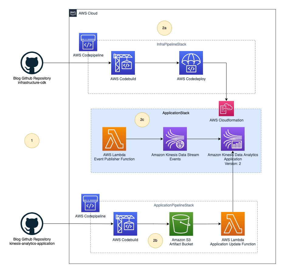
The final solution includes the following steps:

  1. The platform (DevOps) team and data engineering team push their source code to their respective code repositories.
  2. CodePipeline deploys the whole infrastructure as three stacks:
    1. InfraPipelineStack – Contains a pipeline to deploy the overall infrastructure.
    2. ApplicationPipelineStack – Contains a pipeline to build and deploy Kinesis Data Analytics application binaries. In this post, we build a Java source using the JavaBuildPipeline AWS CDK construct. You can use the PythonBuildPipeline AWS CDK construct to build a Python source.
    3. ApplicationStack – Contains real-time data analytics pipeline resources including Lambda (data source), Kinesis Data Streams (storage), and Kinesis Data Analytics (Apache Flink application).

Deploy resources using AWS CDK

The following GitHub repository contains the AWS CDK code to create all the necessary resources for the data pipeline. This removes opportunities for manual error, increases efficiency, and ensures consistent configurations over time. To deploy the resources, complete the following steps:

  1. Clone the GitHub repository to your local computer using the following command:
git clone https://github.com/aws-samples/automate-deployment-and-version-update-of-kda-application
  1. Download and install the latest Node.js.
  2. Run the following command to install the latest version of AWS CDK:
npm install -g aws-cdk
  1. Run cdk bootstrap to initialize the AWS CDK environment in your AWS account. Replace your AWS account ID and Region before running the following command.
cdk bootstrap aws://123456789012/us-east-1

To learn more about the bootstrapping process, refer to Bootstrapping.

Part 1: Data engineering and platform teams push source code to their code repositories

The data engineering and platform teams begin work in their respective code repositories, as illustrated in the following figure.

The data engineering and platform teams begin work in their respective code repositories, as illustrated in the following figure.

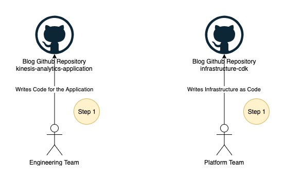
In this post, we use two folders instead of two GitHub repositories, which you can find under the root folder of the cloned repository:

  • kinesis-analytics-application – This folder contains example source code of the Kinesis Data Analytics application. This represents your Kinesis Data Analytics application source code developed by your data engineering team.
  • infrastructure-cdk – This folder contains example AWS CDK source code of the final solution used for provisioning all the required resources and CodePipeline. You can reuse this code for your Kinesis Data Analytics application deployment.

Application development teams usually stores the application source code in git repositories. For the demonstration purpose, we will use source code as zip file downloaded from Github instead of connecting CodePipeline to the Github repository. You may want to directly connect source repository with CodePipeline. To learn more about how to connect, refer to Create a connection to GitHub.

Part 2: The platform team deploys the application pipeline

The following figure illustrates the next step in the workflow.

Next step in the workflow illustrated

In this step, you deploy the first pipeline to build the Java source code from kinesis-analytics-application. Complete the following steps to deploy ApplicationPipelineStack:

  1. Open your terminal, bash, or command window depending on your OS.
  2. Switch the current path to the folder infrastructure-cdk.
  3. Run npm install to download all dependencies.
  4. Run cdk deploy ApplicationPipelineStack to deploy the application pipeline.

This process should take about 5 minutes to complete and deploys the following resources to your AWS account, highlighted in green in the preceding diagram:

  • CodePipeline, containing stages for AWS CodeBuild and AWS CodeDeploy
  • An S3 bucket to store binaries
  • A Lambda function to update the Kinesis Data Analytics application JAR after manual approval

Trigger an automatic build for the application pipeline

After the cdk deploy command is successful, complete the following steps to automatically run the pipeline:

  1. Download the source code .zip file.
  2. On the AWS CloudFormation console, choose Stacks in the navigation pane.
  3. Choose the stack ApplicationPipelineStack.Choose the stack ApplicationPipelineStack.
  4. On the Outputs tab, choose the link for the key ArtifactBucketLink.On the Outputs tab, choose the link for the key ArtifactBucketLink.

You’re redirected to the S3 artifact bucket.

  1. Choose Upload.
  2. Upload the source code .zip file you downloaded.

The first pipeline run (shown as Auto Build in the following diagram) starts automatically and takes about 5 minutes to reach the manual approval stage. The pipeline automatically downloads the source code from the artifact bucket, builds the Java project kinesis-analytics-application using Maven, and publishes the output binary JAR file back to the artifact bucket under the directory jars.

The pipeline automatically downloads the source code from the artifact bucket, builds the Java project kinesis-analytics-application using Maven, and publishes the output binary JAR file back to the artifact bucket under the directory jars.

View the application pipeline run

Complete the following steps to view the application pipeline run:

  1. On the AWS CloudFormation console, navigate to the stack ApplicationPipelineStack.
  2. On the Outputs tab, choose the link for the key ApplicationCodePipelineLink.On the Outputs tab, choose the link for the key ApplicationCodePipelineLink.

You’re redirected to the pipeline details page. You can see a detailed view of the pipeline, including the state of each action in each stage and the state of the transitions.

Do not approve the build for the manual approval stage yet; this is done later.

Part 3: The platform team deploys the infrastructure pipeline

The application pipeline run publishes a JAR file named kinesis-analytics-application-final.jar to the artifact bucket. Next, we deploy the Kinesis Data Analytics architecture. Complete the following steps to deploy the example flow:

  1. Open a terminal, bash, or command window depending on your OS.
  2. Switch the current path to the folder infrastructure-cdk.
  3. Run cdk deploy InfraPipelineStack to deploy the infrastructure pipeline.

This process should take about 5 minutes to complete and deploys a pipeline containing stages for CodeBuild and CodeDeploy to your AWS account, as highlighted in green in the following diagram.

This process should take about 5 minutes to complete and deploys a pipeline containing stages for CodeBuild and CodeDeploy to your AWS account, as highlighted in green in the following diagram.

When the cdk deploy is complete, the infrastructure pipeline run starts automatically (shown as Auto Build 1 in the following diagram) and takes about 10 minutes to download the source code from the artifact bucket, build the AWS CDK project infrastructure-stack, and deploy ApplicationStack automatically to your AWS account. When the infrastructure pipeline run is complete, the following resources are deployed to your account (shown in green in following diagram):

  • A CloudFormation template named app-ApplicationStack
  • A Lambda function acting as a data source
  • A Kinesis data stream acting as the stream storage
  • A Kinesis Data Analytics application with the first version of kinesis-analytics-application-final.jarWhen the infrastructure pipeline run is complete, the following resources are deployed to your account (shown in green in following diagram):

View the infrastructure pipeline run

Complete the following steps to view the application pipeline run:

  1. On the AWS CloudFormation console, navigate to the stack InfraPipelineStack.On the AWS CloudFormation console, navigate to the stack InfraPipelineStack.
  2. On the Outputs tab, choose the link for the key InfraCodePipelineLink.On the Outputs tab, choose the link for the key InfraCodePipelineLink.

You’re redirected to the pipeline details page. You can see a detailed view of the pipeline, including the state of each action in each stage and the state of the transitions.

Step 4: The data engineering team deploys the application

Now your account has everything in place for the data engineering team to work independently and roll out new versions of the Kinesis Data Analytics application. You can approve the respective application build from the application pipeline to deploy new versions of the application. The following diagram illustrates the full workflow.

Diagram illustrates the full workflow.

The build process starts automatically when it detects changes in the source code. You can test a version update by re-uploading the source code .zip file to the S3 artifact bucket. In a real-world use case, you update the main branch either via a pull request or by merging your changes, and this action triggers a new pipeline run automatically.

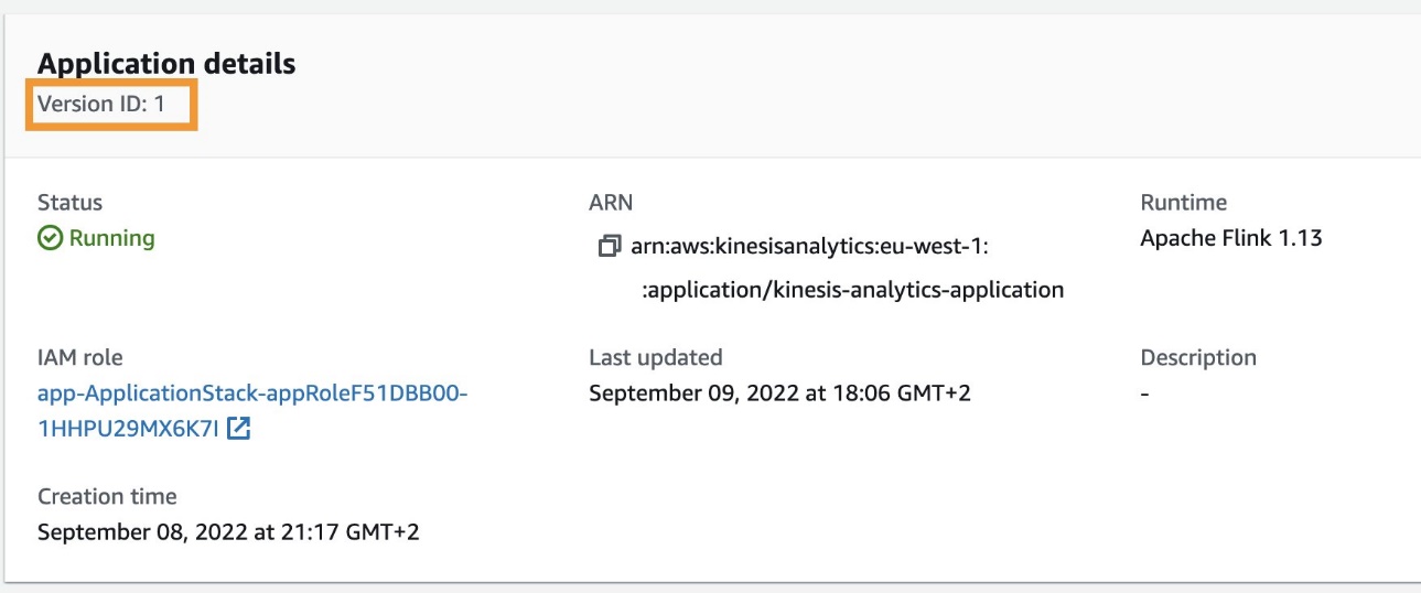
View the current application version

To view the current version of the Kinesis Data Analytics application, complete the following steps:

  1. On the AWS CloudFormation console, navigate to the stack InfraPipelineStack.
  2. On the Outputs tab, choose the link for the key KDAApplicationLink.On the Outputs tab, choose the link for the key KDAApplicationLink.

You’re redirected to the Kinesis Data Analytics application details page. You can find the current application version by looking at Version ID.

Find the current application version by looking at Version ID

Approve the application deployment

Complete the following steps to approve the deployment (or version update) of the Kinesis Data Analytics application:

  1. On the AWS CloudFormation console, navigate to the stack ApplicationPipelineStack.
  2. On the Outputs tab, choose the link for the key ApplicationCodePipelineLink.
  3. Choose Review from the pipeline approval stage.Choose Review from the pipeline approval stage
  4. When prompted, choose Approve to provide approval (optionally adding any comments) for the Kinesis Data Analytics application deployment or version update.Choose Approve to provide approval
  5. Repeat the steps mentioned earlier to view the current application version.

You should see the application version as defined in Version ID increased by one, as shown in the following screenshot.

Application version as defined in Version ID increased by one

Deploying a new version of the Kinesis Data Analytics application will cause a downtime of around 5 minutes because the Lambda function responsible for the version update makes the API call UpdateApplication, which restarts the application after updating the version. However, the application resumes stream processing where it left off after the restart.

Clean up

Complete the following steps to delete your resources and stop incurring costs:

  1. On the AWS CloudFormation console, select the stack InfraPipelineStack and choose Delete.
  2. Select the stack app-ApplicationStack and choose Delete.
  3. Select stack ApplicationPipelineStack and choose Delete.
  4. On the Amazon S3 console, select the bucket with the name starting with javaappCodePipeline and choose Empty.
  5. Enter permanently delete to confirm the choice.
  6. Select the bucket again and choose Delete.
  7. Confirm the action by entering the bucket name when prompted.
  8. Repeat these steps to delete the bucket with the name starting with infrapipelinestack-pipelineartifactsbucket.

Summary

This post demonstrated how to automate deployment and version updates for your Kinesis Data Analytics applications using CodePipeline and AWS CDK.

For more information, see Continuous integration and delivery (CI/CD) using CDK Pipelines and CodePipeline tutorials.


About the Author

About the AuthorAnand Shah is a Big Data Prototyping Solutions Architect at AWS. He works with AWS customers and their engineering teams to build prototypes using AWS analytics services and purpose-built databases. Anand helps customers solve the most challenging problems using the art of the possible technology. He enjoys beaches in his leisure time.

How Plugsurfing doubled performance and reduced cost by 70% with purpose-built databases and AWS Graviton

Post Syndicated from Anand Shah original https://aws.amazon.com/blogs/big-data/how-plugsurfing-doubled-performance-and-reduced-cost-by-70-with-purpose-built-databases-and-aws-graviton/

Plugsurfing aligns the entire car charging ecosystem—drivers, charging point operators, and carmakers—within a single platform. The over 1 million drivers connected to the Plugsurfing Power Platform benefit from a network of over 300,000 charging points across Europe. Plugsurfing serves charging point operators with a backend cloud software for managing everything from country-specific regulations to providing diverse payment options for customers. Carmakers benefit from white label solutions as well as deeper integrations with their in-house technology. The platform-based ecosystem has already processed more than 18 million charging sessions. Plugsurfing was acquired fully by Fortum Oyj in 2018.

Plugsurfing uses Amazon OpenSearch Service as a central data store to store 300,000 charging stations’ information and to power search and filter requests coming from mobile, web, and connected car dashboard clients. With the increasing usage, Plugsurfing created multiple read replicas of an OpenSearch Service cluster to meet demand and scale. Over time and with the increase in demand, this solution started to become cost exhaustive and limited in terms of cost performance benefit.

AWS EMEA Prototyping Labs collaborated with the Plugsurfing team for 4 weeks on a hands-on prototyping engagement to solve this problem, which resulted in 70% cost savings and doubled the performance benefit over the current solution. This post shows the overall approach and ideas we tested with Plugsurfing to achieve the results.

The challenge: Scaling higher transactions per second while keeping costs under control

One of the key issues of the legacy solution was keeping up with higher transactions per second (TPS) from APIs while keeping costs low. The majority of the cost was coming from the OpenSearch Service cluster, because the mobile, web, and EV car dashboards use different APIs for different use cases, but all query the same cluster. The solution to achieve higher TPS with the legacy solution was to scale the OpenSearch Service cluster.

The following figure illustrates the legacy architecture.

Legacy Architecture

Plugsurfing APIs are responsible for serving data for four different use cases:

  • Radius search – Find all the EV charging stations (latitude/longitude) with in x km radius from the point of interest (or current location on GPS).
  • Square search – Find all the EV charging stations within a box of length x width, where the point of interest (or current location on GPS) is at the center.
  • Geo clustering search – Find all the EV charging stations clustered (grouped) by their concentration within a given area. For example, searching all EV chargers in all of Germany results in something like 50 in Munich and 100 in Berlin.
  • Radius search with filtering – Filter the results by EV charger that are available or in use by plug type, power rating, or other filters.

The OpenSearch Service domain configuration was as follows:

  • m4.10xlarge.search x 4 nodes
  • Elasticsearch 7.10 version
  • A single index to store 300,000 EV charger locations with five shards and one replica
  • A nested document structure

The following code shows the example document

{
   "locationId":"location:1",
   "location":{
      "latitude":32.1123,
      "longitude":-9.2523
   },
   "adress":"parking lot 1",
   "chargers":[
      {
         "chargerId":"location:1:charger:1",
         "connectors":[
            {
               "connectorId":"location:1:charger:1:connector:1",
               "status":"AVAILABLE",
               "plug_type":"Type A"
            }
         ]
      }
   ]
}

Solution overview

AWS EMEA Prototyping Labs proposed an experimentation approach to try three high-level ideas for performance optimization and to lower overall solution costs.

We launched an Amazon Elastic Compute Cloud (EC2) instance in a prototyping AWS account to host a benchmarking tool based on k6 (an open-source tool that makes load testing simple for developers and QA engineers) Later, we used scripts to dump and restore production data to various databases, transforming it to fit with different data models. Then we ran k6 scripts to run and record performance metrics for each use case, database, and data model combination. We also used the AWS Pricing Calculator to estimate the cost of each experiment.

Experiment 1: Use AWS Graviton and optimize OpenSearch Service domain configuration

We benchmarked a replica of the legacy OpenSearch Service domain setup in a prototyping environment to baseline performance and costs. Next, we analyzed the current cluster setup and recommended testing the following changes:

  • Use AWS Graviton based memory optimized EC2 instances (r6g) x 2 nodes in the cluster
  • Reduce the number of shards from five to one, given the volume of data (all documents) is less than 1 GB
  • Increase the refresh interval configuration from the default 1 second to 5 seconds
  • Denormalize the full document; if not possible, then denormalize all the fields that are part of the search query
  • Upgrade to Amazon OpenSearch Service 1.0 from Elasticsearch 7.10

Plugsurfing created multiple new OpenSearch Service domains with the same data and benchmarked them against the legacy baseline to obtain the following results. The row in yellow represents the baseline from the legacy setup; the rows with green represent the best outcome out of all experiments performed for the given use cases.

DB Engine Version Node Type Nodes in Cluster Configurations Data Modeling Radius req/sec Filtering req/sec Performance Gain %
Elasticsearch 7.1 m4.10xlarge 4 5 shards, 1 replica Nested 2841 580 0
Amazon OpenSearch Service 1.0 r6g.xlarge 2 1 shards, 1 replica Nested 850 271 32.77
Amazon OpenSearch Service 1.0 r6g.xlarge 2 1 shards, 1 replica Denormalized 872 670 45.07
Amazon OpenSearch Service 1.0 r6g.2xlarge 2 1 shards, 1 replica Nested 1667 474 62.58
Amazon OpenSearch Service 1.0 r6g.2xlarge 2 1 shards, 1 replica Denormalized 1993 1268 95.32

Plugsurfing was able to gain 95% (doubled) better performance across the radius and filtering use cases with this experiment.

Experiment 2: Use purpose-built databases on AWS for different use cases

We tested Amazon OpenSearch Service, Amazon Aurora PostgreSQL-Compatible Edition, and Amazon DynamoDB extensively with many data models for different use cases.

We tested the square search use case with an Aurora PostgreSQL cluster with a db.r6g.2xlarge single node as the reader and a db.r6g.large single node as the writer. The square search used a single PostgreSQL table configured via the following steps:

  1. Create the geo search table with geography as the data type to store latitude/longitude:
CREATE TYPE status AS ENUM ('available', 'inuse', 'out-of-order');

CREATE TABLE IF NOT EXISTS square_search
(
id     serial PRIMARY KEY,
geog   geography(POINT),
status status,
data   text -- Can be used as json data type, or add extra fields as flat json
);
  1. Create an index on the geog field:
CREATE INDEX global_points_gix ON square_search USING GIST (geog);
  1. Query the data for the square search use case:
SELECT id, ST_AsText(geog), status, datafrom square_search
where geog && ST_MakeEnvelope(32.5,9,32.8,11,4326) limit 100;

We achieved an eight-times greater improvement in TPS for the square search use case, as shown in the following table.

DB Engine Version Node Type Nodes in Cluster Configurations Data modeling Square req/sec Performance Gain %
Elasticsearch 7.1 m4.10xlarge 4 5 shards, 1 replica Nested 412 0
Aurora PostgreSQL 13.4 r6g.large 2 PostGIS, Denormalized Single table 881 213.83
Aurora PostgreSQL 13.4 r6g.xlarge 2 PostGIS, Denormalized Single table 1770 429.61
Aurora PostgreSQL 13.4 r6g.2xlarge 2 PostGIS, Denormalized Single table 3553 862.38

We tested the geo clustering search use case with a DynamoDB model. The partition key (PK) is made up of three components: <zoom-level>:<geo-hash>:<api-key>, and the sort key is the EV charger current status. We examined the following:

  • The zoom level of the map set by the user
  • The geo hash computed based on the map tile in the user’s view port area (at every zoom level, the map of Earth is divided into multiple tiles, where each tile can be represented as a geohash)
  • The API key to identify the API user
Partition Key: String Sort Key: String total_pins: Number filter1_pins: Number filter2_pins: Number filter3_pins: Number
5:gbsuv:api_user_1 Available 100 50 67 12
5:gbsuv:api_user_1 in-use 25 12 6 1
6:gbsuvt:api_user_1 Available 35 22 8 0
6:gbsuvt:api_user_1 in-use 88 4 0 35

The writer updates the counters (increment or decrement) against each filter condition and charger status whenever the EV charger status is updated at all zoom levels. With this model, the reader can query pre-clustered data with a single direct partition hit for all the map tiles viewable by the user at the given zoom level.

The DynamoDB model helped us gain a 45-times greater read performance for our geo clustering use case. However, it also added extra work on the writer side to pre-compute numbers and update multiple rows when the status of a single EV charger is updated. The following table summarizes our results.

DB Engine Version Node Type Nodes in Cluster Configurations Data modeling Clustering req/sec Performance Gain %
Elasticsearch 7.1 m4.10xlarge 4 5 shards, 1 replica Nested 22 0
DynamoDB NA Serverless 0 100 WCU, 500 RCU Single table 1000 4545.45

Experiment 3: Use AWS Lambda@Edge and AWS Wavelength for better network performance

We recommended that Plugsurfing use Lambda@Edge and AWS Wavelength to optimize network performance by shifting some of the APIs at the edge to closer to the user. The EV car dashboard can use the same 5G network connectivity to invoke Plugsurfing APIs with AWS Wavelength.

Post-prototype architecture

The post-prototype architecture used purpose-built databases on AWS to achieve better performance across all four use cases. We looked at the results and split the workload based on which database performs best for each use case. This approach optimized performance and cost, but added complexity on readers and writers. The final experiment summary represents the database fits for the given use cases that provide the best performance (highlighted in orange).

Plugsurfing has already implemented a short-term plan (light green) as an immediate action post-prototype and plans to implement mid-term and long-term actions (dark green) in the future.

DB Engine Node Type Configurations Radius req/sec Radius Filtering req/sec Clustering req/sec Square req/sec Monthly Costs $ Cost Benefit % Performance Gain %
Elasticsearch 7.1 m4.10xlarge x4 5 shards 2841 580 22 412 9584,64 0 0
Amazon OpenSearch Service 1.0 r6g.2xlarge x2

1 shard

Nested

1667 474 34 142 1078,56 88,75 -39,9
Amazon OpenSearch Service 1.0 r6g.2xlarge x2 1 shard 1993 1268 125 685 1078,56 88,75 5,6
Aurora PostgreSQL 13.4 r6g.2xlarge x2 PostGIS 0 0 275 3553 1031,04 89,24 782,03
DynamoDB Serverless

100 WCU

500 RCU

0 0 1000 0 106,06 98,89 4445,45
Summary . . 2052 1268 1000 3553 2215,66 76,88 104,23

The following diagram illustrates the updated architecture.

Post Prototype Architecture

Conclusion

Plugsurfing was able to achieve a 70% cost reduction over their legacy setup with two-times better performance by using purpose-built databases like DynamoDB, Aurora PostgreSQL, and AWS Graviton based instances for Amazon OpenSearch Service. They achieved the following results:

  • The radius search and radius search with filtering use cases achieved better performance using Amazon OpenSearch Service on AWS Graviton with a denormalized document structure
  • The square search use case performed better using Aurora PostgreSQL, where we used the PostGIS extension for geo square queries
  • The geo clustering search use case performed better using DynamoDB

Learn more about AWS Graviton instances and purpose-built databases on AWS, and let us know how we can help optimize your workload on AWS.


About the Author

Anand ShahAnand Shah is a Big Data Prototyping Solution Architect at AWS. He works with AWS customers and their engineering teams to build prototypes using AWS Analytics services and purpose-built databases. Anand helps customers solve the most challenging problems using art-of-the-possible technology. He enjoys beaches in his leisure time.

Audit AWS service events with Amazon EventBridge and Amazon Kinesis Data Firehose

Post Syndicated from Anand Shah original https://aws.amazon.com/blogs/big-data/audit-aws-service-events-with-amazon-eventbridge-and-amazon-kinesis-data-firehose/

Amazon EventBridge is a serverless event bus that makes it easy to build event-driven applications at scale using events generated from your applications, integrated software as a service (SaaS) applications, and AWS services. Many AWS services generate EventBridge events. When an AWS service in your account emits an event, it goes to your account’s default event bus.

The following are a few event examples:

By default, these AWS service-generated events are transient and therefore not retained. This post shows how you can forward AWS service-generated events or custom events to Amazon Simple Storage Service (Amazon S3) for long-term storage, analysis, and auditing purposes using EventBridge rules and Amazon Kinesis Data Firehose.

Solution overview

In this post, we provide a working example of AWS service-generated events ingested to Amazon S3. To make sure we have some service events available in default event bus, we use Parameter Store, a capability of AWS Systems Manager to store new parameters manually. This action generates a new event, which is ingested by the following pipeline.

Architecture Diagram

The pipeline includes the following steps:

  1. AWS service-generated events (for example, a new parameter created in Parameter Store) goes to the default event bus at EventBridge.
  2. The EventBridge rule matches all events and forwards those to Kinesis Data Firehose.
  3. Kinesis Data Firehose delivers events to the S3 bucket partitioned by detail-type and receipt time using its dynamic partitioning capability.
  4. The S3 bucket stores the delivered events, and their respective event schema is registered to the AWS Glue Data Catalog using an AWS Glue crawler.
  5. You query events using Amazon Athena.

Deploy resources using AWS CloudFormation

We use AWS CloudFormation templates to create all the necessary resources for the ingestion pipeline. This removes opportunities for manual error, increases efficiency, and provides consistent configurations over time. The template is also available on GitHub.

Complete the following steps:

  1. Click here to
    Launch Stack
  2. Acknowledge that the template may create AWS Identity and Access Management (IAM) resources.
  3. Choose Create stack.

The template takes about 10 minutes to complete and creates the following resources in your AWS account:

  • An S3 bucket to store event data.
  • A Firehose delivery stream with dynamic partitioning configuration. Dynamic partitioning enables you to continuously partition streaming data in Kinesis Data Firehose by using keys within the data (for example, customer_id or transaction_id) and then deliver the data grouped by these keys into corresponding S3 prefixes.
  • An EventBridge rule that forwards all events from the default event bus to Kinesis Data Firehose.
  • An AWS Glue crawler that references the path to the event data in the S3 bucket. The crawler inspects data landed to Amazon S3 and registers tables as per the schema with the AWS Glue Data Catalog.
  • Athena named queries for you to query the data processed by this example.

Trigger a service event

After you create the CloudFormation stack, you trigger a service event.

  1. On the AWS CloudFormation console, navigate to the Outputs tab for the stack.
  2. Choose the link for the key CreateParameter.

Create Parameter

You’re redirected to the Systems Manager console to create a new parameter.

  1. For Name, enter a name (for example, my-test-parameter).
  2. For Value, enter the test value of your choice (for example, test-value).

My Test parameter

  1. Leave everything else as default and choose Create parameter.

This step saves the new Systems Manager parameter and pushes the parameter-created event to the default EventBridge event bus, as shown in the following code:

{
  "version": "0",
  "id": "6a7e4feb-b491-4cf7-a9f1-bf3703497718",
  "detail-type": "Parameter Store Change",
  "source": "aws.ssm",
  "account": "123456789012",
  "time": "2017-05-22T16:43:48Z",
  "region": "us-east-1",
  "resources": [
    "arn:aws:ssm:us-east-1:123456789012:parameter/foo"
  ],
  "detail": {
    "operation": "Create",
    "name": "my-test-parameter",
    "type": "String",
    "description": ""
  }
}

Discover the event schema

After the event is triggered by saving the parameter, wait at least 2 minutes for the event to be ingested via Kinesis Data Firehose to the S3 bucket. Now complete the following steps to run an AWS Glue crawler to discover and register the event schema in the Data Catalog:

  1. On the AWS Glue console, choose Crawlers in the navigation pane.
  2. Select the crawler with the name starting with S3EventDataCrawler.
  3. Choose Run crawler.

Run Crawler

This step runs the crawler, which takes about 2 minutes to complete. The crawler discovers the schema from all events and registers it as tables in the Data Catalog.

Query the event data

When the crawler is complete, you can start querying event data. To query the event, complete the following steps:

  1. On the AWS CloudFormation console, navigate to the Outputs tab for your stack.
  2. Choose the link for the key AthenaQueries.

Athena Queries

You’re redirected to the Saved queries tab on the Athena console. If you’re running Athena queries for the first time, set up your S3 output bucket. For instructions, see Working with Query Results, Recent Queries, and Output Files.

  1. Search for Blog to find the queries created by this post.
  2. Choose the query Blog – Query Parameter Store Events.

Find Athena Saved Queries

The query opens on the Athena console.

  1. Choose Run query.

You can update the query to search the event you created earlier.

  1. Apply a WHERE clause with the parameter name you selected earlier:
SELECT * FROM "AwsDataCatalog"."eventsdb-randomId"."parameter_store_change"
WHERE detail.name = 'Your event name'

You can also choose the link next to the key CuratedBucket from the CloudFormation stack outputs to see paths and the objects loaded to the S3 bucket from other event sources. Similarly, you can query them via Athena.

Clean up

Complete the following steps to delete your resources and stop incurring costs:

  1. On the AWS CloudFormation console, select the stack you created and choose Delete.
  2. On the Amazon S3 console, find the bucket with the name starting with eventbridge-firehose-blog-curatedbucket.
  3. Select the bucket and choose Empty.
  4. Enter permanently delete to confirm the choice.
  5. Select the bucket again and choose Delete.
  6. Confirm the action by entering the bucket name when prompted.
  7. On the Systems Manager console, go to the parameter store and delete the parameter you created earlier.

Summary

This post demonstrates how to use an EventBridge rule to redirect AWS service-generated events or custom events to Amazon S3 using Kinesis Data Firehose to use for long-term storage, analysis, querying, and audit purposes.

For more information, see the Amazon EventBridge User Guide. To learn more about AWS service events supported by EventBridge, see Events from AWS services.


About the Author

Anand ShahAnand Shah is a Big Data Prototyping Solution Architect at AWS. He works with AWS customers and their engineering teams to build prototypes using AWS analytics services and purpose-built databases. Anand helps customers solve the most challenging problems using the art of the possible technology. He enjoys beaches in his leisure time.

Load CDC data by table and shape using Amazon Kinesis Data Firehose Dynamic Partitioning

Post Syndicated from Anand Shah original https://aws.amazon.com/blogs/big-data/load-cdc-data-by-table-and-shape-using-amazon-kinesis-data-firehose-dynamic-partitioning/

Amazon Kinesis Data Firehose is the easiest way to reliably load streaming data into data lakes, data stores, and analytics services. Customers already use Amazon Kinesis Data Firehose to ingest raw data from various data sources using direct API call or by integrating Kinesis Data Firehose with Amazon Kinesis Data Streams including “change data capture” (CDC) use case.

Customers typically use single Kinesis Data Stream per business domain to ingest CDC data. For example, related fact and dimension tables change data is sent to the same stream. Once the data is loaded to Amazon S3, customers use ETL tools to split the data by tables, shape, and desired partitions as the first step in the data enrichment process.

This post demonstrates how customers can use Amazon Kinesis Firehose Dynamic Partitioning to split the data by table, shape (by message schema/version), and by desired partitions on the fly to do this first step of data enrichment while ingesting data.

Solution Overview

In this post, we provide a working example of a CDC pipeline where fake customer, order, and transaction table data is pushed from the source and registered as tables to the AWS Glue Data Catalog. The following architecture diagram illustrates this overall flow. We are using AWS Lambda to generate test CDC data for this post. However, in the real world you would use AWS Data Migration Service (DMS) or a similar tool to push change data to the Amazon Kinesis Data Stream.

The workflow includes the following steps:

  1. An Amazon EventBridge event triggers an AWS Lambda function every minute.
  2. The Lambda function generates test transactions, customers and order CDC data, as well as sends the data to Amazon Kinesis Data Stream.
  3. Amazon Kinesis Data Firehose reads data from Amazon Kinesis Data Stream.
  4. Amazon Kinesis Data Firehose
    1. Applies Dynamic Partitioning configuration defined in the Firehose configuration
    2. Invokes AWS Lambda transform to derive custom Dynamic Partitioning.
  5. Amazon Kinesis Data Firehose saves data to Amazon Simple Storage Service (S3) bucket.
  6. The user runs queries on Amazon S3 bucket data using Amazon Athena, which internally uses the AWS Glue Data Catalog to supply meta data.

Deploying using AWS CloudFormation

You use CloudFormation templates to create all of the necessary resources for the data pipeline. This removes opportunities for manual error, increases efficiency, and ensures consistent configurations over time.

Steps to follow:

  1. Click here to Launch Stack:
  2. Acknowledge that the template may create AWS Identity and Access Management (IAM) resources.
  3. Choose Create stack.

This CloudFormation template takes about five minutes to complete and creates the following resources in your AWS account:

  • An S3 bucket to store ingested data
  • Lambda function to publish test data
  • Kinesis Data Stream connected to Kinesis Data Firehose
  • A Lambda function to compute custom dynamic partition for Kinesis Data Firehose transform
  • AWS Glue Data Catalog tables and Athena named queries for you to query data processed by this example

Once the AWS CloudFormation stack creation is successful, you should be able to see data automatically arriving to Amazon S3 in about five more minutes.

Data sources input

The Lambda function automatically publishes four types of messages to the Kinesis Data Stream at regular intervals with random data when invoked in the following format. In this example, we use three tables:

  • Customers: Has basic customer details.
  • Orders: Mimics orders placed by customers on the shopping website or mobile app.
  • Transactions: Mimics payment transaction done for the order. The transaction table showcases possible message schema evolution that can happen over time from message schema v1 to v2. It also shows how you can split messages by schema version if you don’t want to merge them into a universal schema.

Customer table sample message

{
   "version": 1,
   "table": "Customer",
   "data": {
        "id": 1,
        "name": "John",
        "country": "US"
   }
}

Orders table sample message

{
   "version": 1,
   "table": "Order",
   "data": {
        "id": 1,
        "customerId": 1,
        "qty": 1,
        "product": {
            "name": "Book 54",
            "price": 12.6265
        }
   }
}

Transactions in old message format (v1)

{
    "version": 1, 
    "txid": "52", 
    "amount": 32.6516
}

Transactions in new message format (v2 – latest)

This message example demonstrates message evolution over time. txid from old message format is now renamed to transactionId, and new information like source is added to the original old transaction message in the new message version v2.

{
   "version": 2,
   "transactionId": "52",
   "amount": 32.6516,
   "source": "Web"
}

Dynamic Partitioning Logic

Amazon Kinesis Data Firehose dynamic partitioning configuration is defined using jq style syntax. We will use the table field for the first partition and the version field for the second level partition. We can derive the table partition using dynamic partitioning jq syntax “.version”. As you can see, the version field is available in all of the messages. Therefore, we can use it directly in partitioning. However, the table field is not available for old and new transaction messages. Therefore, we derive the table field using custom transform Lambda function.

We check the existence of the table field from the incoming message and populate it with the static value “Transaction” if table field is not present. Lambda function also returns PartitionKeys for Kinesis Data Firehose to use as dynamic partition. The Lambda function also derives the year, month, and day from the current time.

for firehose_record_input in firehose_records_input['records']:
    # Get user payload
    payload = base64.b64decode(firehose_record_input['data'])
    json_value = json.loads(payload)


    # Create output Firehose record and add modified payload and record ID to it.
    firehose_record_output = {}

    table = "Transaction"
    if "table" in json_value:
        table = json_value["table"]

    now = datetime.datetime.now()
    partition_keys = {"table": table, "year": str(now.year), "month": str(now.month), "day": str(now.day)}

The Kinesis Data Firehose S3 destination Prefix is set to table=!{partitionKeyFromLambda:table}/version=!{partitionKeyFromQuery:version}/year=!{partitionKeyFromLambda:year}/month=!{partitionKeyFromLambda:month}/day=!{partitionKeyFromLambda:day}/

  • table partition key is coming from the Lambda function based on custom logic.
  • version partition key is extracted using jq expression using Kinesis Data Firehose dynamic partition configuration. Here, the version refers to the shape of the message and not the version of the data. For example, Updates to Customer record with same ID is not merged into one.
  • year, month, and day partition keys are coming from the Lambda function based on current time

You can follow the respective links from the CloudFormation stack Output tab to deep dive into the Kinesis Data Firehose configuration, record transformer Lambda function source code, and see output files in the Amazon S3 curated bucket. The entire code is also available in the GitHub repository.

Ingested data output

Kinesis Data Firehose processes all the messages and outputs result in the following S3 hive style partitioned paths:

# AWS Glue Data Catalog table transactions_v1
s3://curated-bucket/table=transaction/version=1/year=2021/month=9/day=20/file-name.gz
# AWS Glue Data Catalog table transactions
s3://curated-bucket/table=transaction/version=2/year=2021/month=9/day=20/file-name.gz
# AWS Glue Data Catalog table customers
s3://curated-bucket/table=customer/version=1/year=2021/month=9/day=20/file-name.gz
# Glue catalog table orders
s3://curated-bucket/table=order/version=1/year=2021/month=9/day=20/file-name.gz

Query output data stored in Amazon S3

Kinesis Data Firehose loads new data every minute to the Amazon S3 bucket, and the associated tables are already created by CloudFormation for you in the AWS Glue Data Catalog. You can directly query Amazon S3 bucket data using the following steps:

  1. Go to Amazon Athena service and select the database with the same name as the CloudFormation stack name without dashes.
  2. Select the three dots next to each table name to open the table menu and select Load Partitions. This will add a new partition to the AWS Glue Data Catalog.
  3. Go to the CloudFormation stack Output tab.
  4. Select the link mentioned next to the key AthenaQueries.
  5. This will take you to the Amazon Athena saved query console. Type the word Blog to search named queries created by this blog.
  6. Select the query called “Blog – Query Customer Orders”. This will open the query in the Athena query console. Select Run query to see the results.
  7. Select the Saved queries menu from the top bar to go back to the Amazon Athena saved query console. Repeat the steps for other Blog queries to see results from the “new and old transactions” queries.

Clean up

Complete the following steps to delete your resources and stop incurring costs:

  1. Go to the CloudFormation stack Output tab.
  2. Select the link mentioned next to the key PauseDataSource. This will take you to the Amazon EventBridge event rules console.
  3. Select the Actions button from the top right menu bar and select Disable.
  4. Confirm the choice by clicking the Disable button again on the prompt. This will disable Amazon EventBridge event trigger that invokes the data generator Lambda function. This lets us make sure that no new data is sent to the Kinesis data stream by Lambda from now onward.
  5. Wait for at least two minutes for all of the buffered events to reach to the S3 from the Kinesis Data Firehose.
  6. Go back to the CloudFormation stack Output tab.
  7. Select the link mentioned next to the key S3BucketCleanup.

You’re redirected to the Amazon S3 console.

  1. Enter permanently delete to delete all of the objects in your S3 bucket.
  2. Choose Empty.
  3. On the AWS CloudFormation console, select the stack you created and choose Delete.

Summary

This post demonstrates how to use the Kinesis Data Firehose Dynamic Partitioning feature to load CDC data on the fly in near real-time. It also shows how we can split CDC data by table and message schema version for backward compatibility and quick query capability. To learn more about dynamic partitioning, you can refer to this blog and this documentation. Provide us with any feedback you have about the new feature.


About the Author

Anand Shah is a Big Data Prototyping Solution Architect at AWS. He works with AWS customers and their engineering teams to build prototypes using AWS Analytics services and purpose-built databases. Anand helps customers solve the most challenging problems using the art of the possible technology. He enjoys beaches in his leisure time.