All posts by Christopher Patton

Prepping for post-quantum: a beginner’s guide to lattice cryptography

2025-03-21 Christopher Patton

Post Syndicated from Christopher Patton original https://blog.cloudflare.com/lattice-crypto-primer/

The cryptography that secures the Internet is evolving, and it’s time to catch up. This post is a tutorial on lattice cryptography, the paradigm at the heart of the post-quantum (PQ) transition.

Twelve years ago (in 2013), the revelation of mass surveillance in the US kicked off the widespread adoption of TLS for encryption and authentication on the web. This transition was buoyed by the standardization and implementation of new, more efficient public-key cryptography based on elliptic curves. Elliptic curve cryptography was both faster and required less communication than its predecessors, including RSA and Diffie-Hellman over finite fields.

Today’s transition to PQ cryptography addresses a looming threat for TLS and beyond: once built, a sufficiently large quantum computer can be used to break all public-key cryptography in use today. And we continue to see advancements in quantum-computer engineering that bring us closer to this threat becoming a reality.

Fortunately, this transition is well underway. The research and standards communities have spent the last several years developing alternatives that resist quantum cryptanalysis. For its part, Cloudflare has contributed to this process and is an early adopter of newly developed schemes. In fact, PQ encryption has been available at our edge since 2022 and is used in over 35% of non-automated HTTPS traffic today (2025). And this year we’re beginning a major push towards PQ authentication for the TLS ecosystem.

Lattice-based cryptography is the first paradigm that will replace elliptic curves. Apart from being PQ secure, lattices are often as fast, and sometimes faster, in terms of CPU time. However, this new paradigm for public key crypto has one major cost: lattices require much more communication than elliptic curves. For example, establishing an encryption key using lattices requires 2272 bytes of communication between the client and the server (ML-KEM-768), compared to just 64 bytes for a key exchange using a modern elliptic-curve-based scheme (X25519). Accommodating such costs requires a significant amount of engineering, from dealing with TCP packet fragmentation, to reworking TLS and its public key infrastructure. Thus, the PQ transition is going to require the participation of a large number of people with a variety of backgrounds, not just cryptographers.

The primary audience for this blog post is those who find themselves involved in the PQ transition and want to better understand what’s going on under the hood. However, more fundamentally, we think it’s important for everyone to understand lattice cryptography on some level, especially if we’re going to trust it for our security and privacy.

We’ll assume you have a software-engineering background and some familiarity with concepts like TLS, encryption, and authentication. We’ll see that the math behind lattice cryptography is, at least at the highest level, not difficult to grasp. Readers with a crypto-engineering background who want to go deeper might want to start with the excellent tutorial by Vadim Lyubashevsky on which this blog post is based. We also recommend Sophie Schmieg’s blog on this subject.

While the transition to lattice cryptography incurs costs, it also creates opportunities. Many things we can build with elliptic curves we can also build with lattices, though not always as efficiently; but there are also things we can do with lattices that we don’t know how to do efficiently with anything else. We’ll touch on some of these applications at the very end.

We’re going to cover a lot of ground in this post. If you stick with it, we hope you’ll come away feeling empowered, not only to tackle the engineering challenges the PQ transition entails, but to solve problems you didn’t know how to solve before.

Strap in — let’s have some fun!

Encryption

The most pressing problem for the PQ transition is to ensure that tomorrow’s quantum computers don’t break today’s encryption. An attacker today can store the packets exchanged between your laptop and a website you visit, and then, some time in the future, decrypt those packets with the help of a quantum computer. This means that much of the sensitive information transiting the Internet today — everything from API tokens and passwords to database encryption keys — may one day be unlocked by a quantum computer.

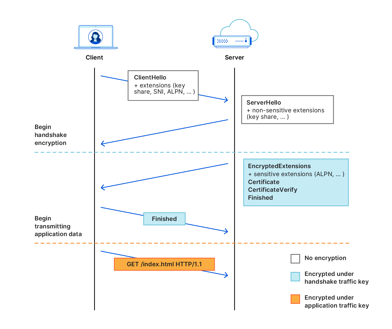
In fact, today’s encryption in TLS is mostly PQ secure: what’s at risk is the process by which your browser and a server establish an encryption key. Today this is usually done with elliptic-curve-based schemes, which are not PQ secure; our goal for this section is to understand how to do key exchange with lattices-based schemes, which are.

We will work through and implement a simplified version of ML-KEM, a.k.a. Kyber, the most widely deployed PQ key exchange in use today. Our code will be less efficient and secure than a spec-compliant, production-quality implementation, but will be good enough to grasp the main ideas.

Our starting point is a protocol that looks an awful lot like Diffie-Hellman (DH) key exchange. For those readers unacquainted with DH, the goal is for Alice and Bob to establish a shared secret over an insecure network. To do so, each picks a random secret number, computes the corresponding “key share”, and sends the key share to the other:

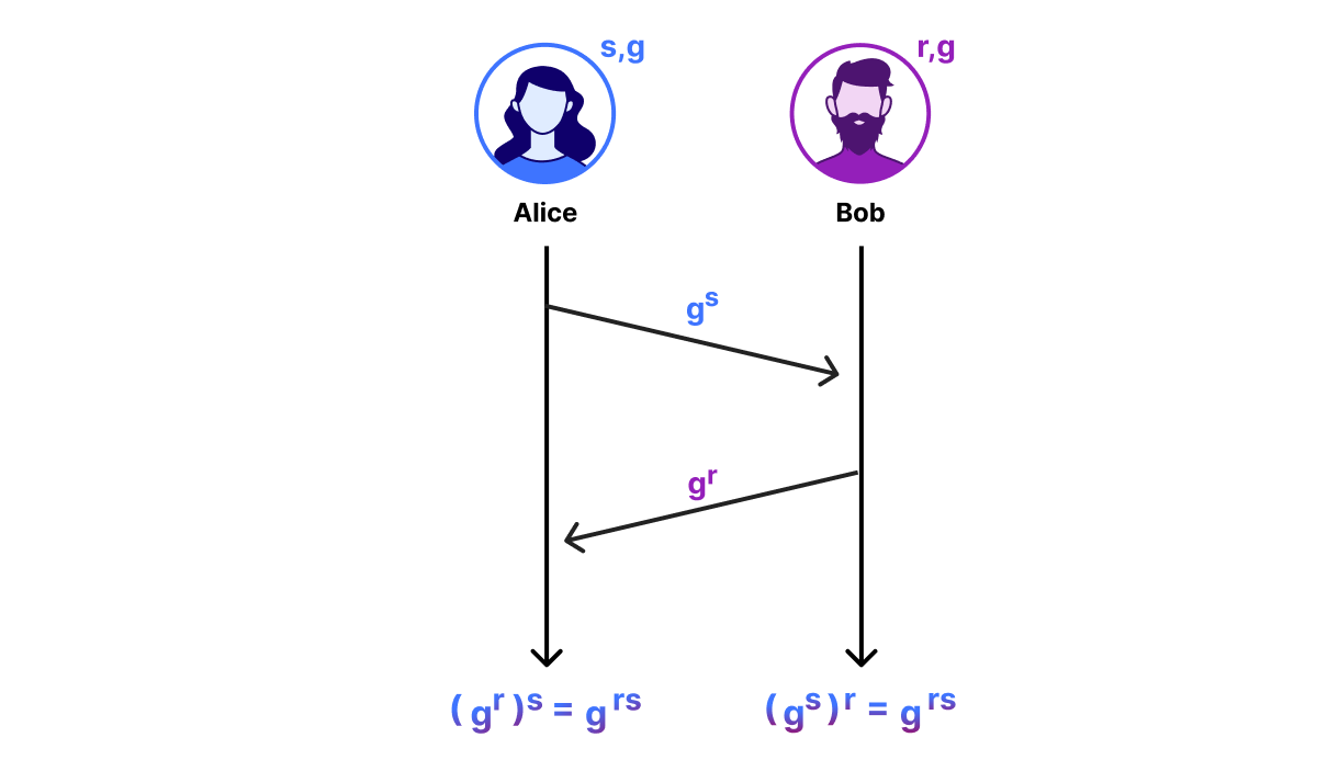
Alice’s secret number is $s$ and her key share is $g^s$; Bob’s secret number is $r$ and his key share is $g^r$. Then given their secret and their peer’s key share, each can compute $g^{rs}$. The security of this protocol comes from how we choose $g$, $s$, and $r$ and how we do arithmetic. The most efficient instantiation of DH uses elliptic curves.

In ML-KEM we replace operations on elliptic curves with matrix operations. It’s not quite a drop-in replacement, so we’ll need a little linear algebra to make sense of it. But don’t worry: we’re going to work with Python so we have running code to play with, and we’ll use NumPy to keep things high level.

All the math we’ll need

A matrix is just a two-dimensional array of numbers. In NumPy, we can create a matrix as follows (importing numpy as np):

A = np.matrix([[1, 2, 3],
               [4, 5, 6],
               [7, 8, 9]])

This defines A to be the 3-by-3 matrix with entries A[0,0]==1, A[0,1]==2, A[0,2]==3, A[1,0]==4, and so on.

For the purposes of this post, the entries of our matrices will always be integers. Furthermore, whenever we add, subtract, or multiply two integers, we then reduce the result, just like we do with hours on a clock, so that we end up with a number in range(Q) for some positive number Q, called the modulus. The exact value doesn’t really matter now, but for ML-KEM it’s Q=3329, so let’s go with that for now. (The modulus for a clock would be Q=12.)

In Python, we write multiplication of integers a and b modulo Q as c = a*b % Q. Here we compute a*b, divide the result by Q, then set c to the remainder. For example, 42*1337 % Q is equal to 2890 rather than 56154. Modular addition and subtraction are done analogously. For the rest of this blog, we will sometimes omit “% Q” when it’s clear in context that we mean modular arithmetic.

Next, we’ll need three operations on matrices.

The first is matrix transpose, written A.T in NumPy. This operation flips the matrix along its diagonal so that A.T[j,i] == A[i,j] for all rows i and columns j:

print(A.T)
# [[1 4 7]
#  [2 5 8]
#  [3 6 9]]

To visualize this, imagine writing down a matrix on a translucent piece of paper. Draw a line from the top left corner to the bottom right corner of that paper, then rotate the paper 180° around that line:

The second operation we’ll need is matrix multiplication. Normally, we will multiply a matrix by a column vector, which is just a matrix with one column. For example, the following 3-by-1 matrix is a column vector:

s = np.matrix([[0],
               [1],
               [0]])

We can also write s more concisely as np.matrix([[0,1,0]]).T. To multiply a square matrix A by a column vector s, we compute the dot product of each row of A with s. That is, if t = A*s % Q, then t[i] == (A[i,0]*s[0,0] + A[i,1]*s[1,0] + A[i,2]*s[2,0]) % Q for each row i. The output will always be a column vector:

print(A*s % Q)
# [[2]
#  [5]
#  [8]]

The number of rows of this column vector is equal to the number of rows of the matrix on the left hand side. In particular, if we take our column vector s, transpose it into a 1-by-3 matrix, and multiply it by a 3-by-1 matrix r, then we end up with a 1-by-1 matrix:

r = np.matrix([[1,2,3]]).T
print(s.T*r % Q)
# [[2]]

The final matrix operation we’ll need is matrix addition. If A and B are both N-by-M matrices, then C = (A+B) % Q is the N-by-M matrix for which C[i,j] == (A[i,j]+B[i,j]) % Q. Of course, this only works if the matrices we’re adding have the same dimensions.

Warm up

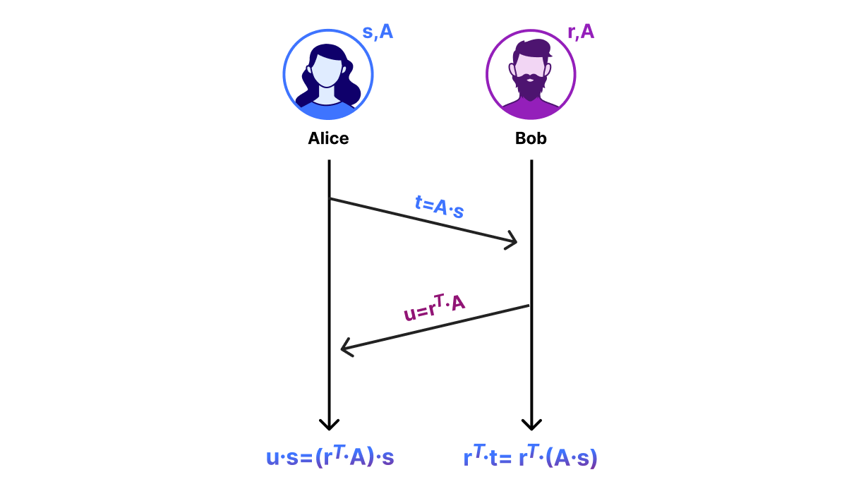
Enough maths — let’s get to exchanging some keys. We start with the DH diagram from before and swap out the computations with matrix operations. Note that this protocol is not secure, but will be the basis of a secure key exchange mechanism we’ll develop in the next section:

Alice and Bob agree on a public, N-by-N matrix A. This is analogous to the number $g$ that Alice and Bob agree on in the DH diagram.
Alice chooses a random length-N vector s and sends t = A*s % Q to Bob.
Bob chooses a random length-N vector r and sends u = r.T*A % Q to Alice. You can also compute this as (A.T*r).T % Q.

The vectors t and u are analogous to DH key shares. After the exchange of these key shares, Alice and Bob can compute a shared secret. Alice computes the shared secret as u*s % Q and Bob computes the shared secret as r.T*t % Q. To see why they compute the same key, notice that u*s == (r.T*A)*s == r.T*(A*s) == r.T*t.

In fact, this key exchange is essentially what happens in ML-KEM. However, we don’t use this directly, but rather as part of a public key encryption scheme. Public key encryption involves three algorithms:

key_gen(): The key generation algorithm that outputs a public encryption key pk and the corresponding secret decryption key sk.
encrypt(): The encryption algorithm that takes the public key and a plaintext and outputs a ciphertext.
decrypt(): The decryption algorithm that takes the secret key and a ciphertext and outputs the underlying plaintext. That is, decrypt(sk, encrypt(pk, ptxt)) == ptxt for any plaintext ptxt.

We’ll say the scheme is secure if, given a ciphertext and the public key used to encrypt it, no attacker can discern any information about the underlying plaintext without knowledge of the secret key. Once we have this encryption scheme, we then transform it into a key-encapsulation mechanism (the “KEM” in “ML-KEM”) in the last step. A KEM is very similar to encryption except that the plaintext is always a randomly generated key.

Our encryption scheme is as follows:

key_gen(): To generate a key pair, we choose a random, square matrix A and a random column vector s. We set our public key to (A,t=A*s % Q) and our secret key to s. Notice that t is Alice’s key share from the key exchange protocol above.
encrypt(): Suppose our plaintext ptxt is an integer in range(Q). To encrypt ptxt, Bob generates his key share u. He then derives the shared secret and adds it to ptxt. The ciphertext has two components:

u = r.T*A % Q

v = (r.T*t + m) % Q

Here m is a 1-by-1 matrix containing the plaintext, i.e., m = np.matrix([[ptxt]]), and r is a random column vector.

decrypt(): To decrypt, Alice computes the shared secret and subtracts it from v:

m = (v - u*s) % Q

Some readers will notice that this looks an awful lot like El Gamal encryption. This isn’t a coincidence. Good cryptographers roll their own crypto; great cryptographers steal from good cryptographers.

Let’s now put this together into code. The last thing we’ll need is a method of generating random matrices and column vectors. We call this function gen_mat() below. Take a crack at implementing this yourself. Our scheme has two parameters: the modulus Q; and the dimension of N of the matrix and column vectors. The choice of N matters for security, but for now feel free to pick whatever value you want.

def key_gen():
    # Here `gen_mat()` returns an N-by-N matrix with entries
    # randomly chosen from `range(0, Q)`.
    A = gen_mat(N, N, 0, Q)
    # Like above except the matrix is N-by-1.
    s = gen_mat(N, 1, 0, Q)
    t = A*s % Q
    return ((A, t), s)

def encrypt(pk, ptxt):
    (A, t) = pk
    m = np.matrix([[ptxt]])
    r = gen_mat(N, 1, 0, Q)
    u = r.T*A % Q
    v = (r.T*t + m) % Q
    return (u, v)

def decrypt(sk, ctxt):
    s = sk
    (u, v) = ctxt
    m = (v - u*s) % Q
    return m[0,0]

# Test
assert decrypt(sk, encrypt(pk, 1)) == 1

Making the scheme secure (or “What is a lattice?”)

By now, you might be wondering what on Earth a lattice even is. We promise we’ll define it, but before we do, it’ll help to understand why our warm-up scheme is insecure and what it’ll take to fix it.

Readers familiar with linear algebra may already see the problem: in order for this scheme to be secure, it should be impossible for the attacker to recover the secret key s; but given the public (A,t), we can immediately solve for s using Gaussian elimination.

In more detail, if A is invertible, we can write the secret key as A^-1*t == A^-1*(A*s) == (A^-1*A)*s == s, where A^-1 is the inverse of A. (When you multiply a matrix by its inverse, you get the identity matrix I, which simply takes a column vector to itself, i.e., I*s == s.) We can use Gaussian elimination to compute this matrix. Intuitively, all we’re doing is solving a set of linear equations, where the entries of s are the unknown variables. (Note that this is possible even if A is not invertible.)

In order to make this encryption scheme secure, we need to make it a little… “messier”.

Let’s get messy

For starters, we need to make it hard to recover the secret key from the public key. Let’s try the following: generate another random vector e and add it into A*s. Our key generation algorithm becomes:

def key_gen():
    A = gen_mat(N, N, 0, Q)
    s = gen_mat(N, 1, 0, Q)
    e = gen_mat(N, 1, 0, Q)
    t = (A*s + e) % Q
    return ((A, t), s)

Our formula for the column vector component of the public key, t, now includes an additive term e, which we’ll call the error. Like the secret key, the error is just a random vector.

Notice that the previous attack no longer works: since A^-1*t == A^-1*(A*s + e) == A^-1*(A*s) + A^-1*e == s + A^-1*e, we need to know e in order to compute s.

Great, but this patch creates another problem. Take a second to plug in this new key generation algorithm into your implementation and test it out. What happens?

You should see that decrypt() now outputs garbage. We can see why using a little algebra:

(v - u*s) == (r.T*t + m) - (r.T*A)*s

                == r.T*(A*s + e) + m - (r.T*A)*s

                == r.T*(A*s) + r.T*e + m - r.T*(A*s)

                == r.T*e + m

The entries of r and e are sampled randomly, so r.T*e is also uniformly random. It’s as if we encrypted m with a one-time pad, then threw away the one-time pad!

Handling decryption errors

What can we do about this? First, it would help if r.T*e were small so that decryption yields something that’s close to the plaintext. Imagine we could generate r and e in such a way that r.T*e were in range(-epsilon, epsilon+1) for some small epsilon. Then decrypt would output a number in range(ptxt-epsilon, ptxt+epsilon+1), which would be pretty close to the actual plaintext.

However, we need to do better than get close. Imagine your browser failing to load your favorite website one-third of the time because of a decryption error. Nobody has time for that.

ML-KEM reduces the probability of decryption errors by being clever about how we encode the plaintext. Suppose all we want to do is encrypt a single bit, i.e., ptxt is either 0 or 1. Consider the numbers in range(Q), and split the number line into four chunks of roughly equal length:

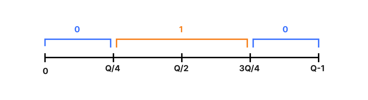
Here we’ve labeled the region around zero (-Q/4 to Q/4 modulo Q) with ptxt=0 and the region far away from zero with ptxt=1. To encode the bit, we set it to the integer corresponding to the middle of its range, i.e., m = np.matrix([[ptxt * Q//2]]). (Note the double “//” — this denotes integer division in Python.) To decode, we choose the ptxt corresponding to whatever range m[0,0] is in. That way if the decryption error is small, then we’re highly likely to end up in the correct range.

Now all that’s left is to ensure the decryption error, r.T*e, is small. We do this by sampling short vectors r and e. By “short” we mean the entries of these vectors are sampled from a range that is much smaller than range(Q). In particular, we’ll pick some small positive integer beta and sample entries range(-beta,beta+1).

How do we choose beta? Well, it should be small enough that decryption succeeds with overwhelming probability, but not so small that r and e are easy to guess and our scheme is broken. Take a minute or two to play with this. The parameters we can vary are:

the modulus Q
the dimension of the column vectors N
the shortness parameter beta

For what ranges of these parameters is the decryption error low but the secret vectors are hard to guess? For what ranges is our scheme most efficient, in terms of runtime and communication cost (size of the public key plus the ciphertext)? We’ll give a concrete answer at the end of this section, but in the meantime, we encourage you to play with this a bit.

Gauss strikes back

At this point, we have a working encryption scheme that mitigates at least one key-recovery attack. We’ve come pretty far, but we have at least one more problem.

Take another look at our formula for the ciphertext ctxt = (u,v). What would happen if we managed to recover the random vector r? That would be catastrophic, since v == r.T*t + m, and we already know t (part of the public key) and v (part of the ciphertext).

Just as we were able to compute the secret key from the public key in our initial scheme, we can recover the encryption randomness r from the ciphertext component u using Gaussian elimination. Again, this is just because r is the solution to a system of linear equations.

We can mitigate this plaintext-recovery attack just as before, by adding some noise. In particular, we’ll generate a short vector according to gen_mat(N,1,-beta,beta+1) and add it into u. We also need to add noise to v in the same way, for reasons that we’ll discuss in the next section.

Once again, adding noise increases the probability of a decryption error, but this time the magnitude of the error also depends on the secret key s. To see this, recall that during decryption, we multiply u by s (to compute the shared secret), and the error vector is an additive term. We’ll therefore need s to be a short vector as well.

Let’s now put together everything we’ve learned into an updated encryption scheme. Our scheme now has three parameters, Q, N, and beta, and can be used to encrypt a single bit:

def key_gen():
    A = gen_mat(N, N, 0, Q)
    s = gen_mat(N, 1, -beta, beta+1)
    e1 = gen_mat(N, 1, -beta, beta+1)
    t = (A*s + e1) % Q
    return ((A, t), s)

def encrypt(pk, ptxt):
    (A, t) = pk
    m = np.matrix([[ptxt*(Q//2) % Q]])
    r = gen_mat(N, 1, -beta, beta+1)
    e2 = gen_mat(N, 1, -beta, beta+1)
    e3 = gen_mat(1, 1, -beta, beta+1)
    u = (r.T*A + e2) % Q
    v = (r.T*t + e3 + m) % Q
    return (u, v)

def decrypt(sk, ctxt):
    s = sk
    (u, v) = ctxt
    m = (v - u*s) % Q
    if m[0,0] in range(Q//4, 3*Q//4):
        return 1
    return 0

# Test
assert decrypt(sk, encrypt(pk, 0)) == 0
assert decrypt(sk, encrypt(pk, 1)) == 1

Before moving on, try to find parameters for which the scheme works and for which the secret and error vectors seem hard to guess.

Learning with errors

So far we have a functioning encryption scheme for which we’ve mitigated two attacks, one a key-recovery attack and the other a plaintext-recovery attack. There seems to be no other obvious way of breaking our scheme, unless we choose parameters that are so weak that an attacker can easily guess the secret key s or ciphertext randomness r. Again, these vectors need to be short in order to prevent decryption errors, but not so short that they are easy to guess. (Likewise for the error terms.)

Still, there may be other attacks that require a little more sophistication to pull off. For instance, there might be some mathematical analysis we can do to recover, or at least make a good guess of, a portion of the ciphertext randomness. This raises a more fundamental question: in general, how do we establish that cryptosystems like this are actually secure?

As a first step, cryptographers like to try and reduce the attack surface. Modern cryptosystems are designed so that the problem of attacking the scheme reduces to solving some other problem that is easier to reason about.

Our public key encryption scheme is an excellent illustration of this idea. Think back to the key- and plaintext-recovery attacks from the previous section. What do these attacks have in common?

In both instances, the attacker knows some public vector that allowed it to recover a secret vector:

In the key-recovery attack, the attacker knew t for which A*s == t.
In the plaintext-recovery attack, the attacker knew u for which r.T*A == u (or, equivalently, A.T*r == u.T).

The fix in both cases was to construct the public vector in such a manner that it is hard to solve for the secret, namely, by adding an error term. However, ideally the public vector would reveal no information about the secret whatsoever. This ideal is formalized by the Learning With Errors (LWE) problem.

The LWE problem asks the attacker to distinguish between two distributions. Concretely, imagine we flip a coin, and if it comes up heads, we sample from the first distribution and give the sample to the attacker; and if the coin comes up tails, we sample from the second distribution and give the sample to the attacker. The distributions are as follows:

(A,t=A*s + e) where A is a random matrix generated with gen_mat(N,N,0,Q) and s and e are short vectors generated with gen_mat(N,1,-beta,beta+1).
(A,t) where A is a random matrix generated with gen_mat(N,N,0,Q) and t is a random vector generated with gen_mat(N,1,0,Q).

The first distribution corresponds to what we actually do in the encryption scheme; in the second, t is just a random vector, and no longer a secret vector at all. We say that the LWE problem is “hard” if no attacker is able to guess the coin flip with probability significantly better than one-half.

Our encryption is passively secure — meaning the ciphertext doesn’t leak any information about the plaintext — if the LWE problem is hard for the parameters we chose. To see why, notice that both the public key and ciphertext look like LWE instances; if we can replace each instance with an instance of the random distribution, then the ciphertext would be completely independent of the plaintext and therefore leak no information about it at all. Note that, for this argument to go through, we also have to add the error term e3 to the ciphertext component v.

Choosing the parameters

We’ve established that if solving the LWE problem is hard for parameters N, Q, and beta, then so is breaking our public key encryption scheme. What’s left for us to do is tune the parameters so that solving LWE is beyond the reach of any attacker we can think of. This is where lattices come in.

Lattices

A lattice is an infinite grid of points in high-dimensional space. A two-dimensional lattice might look something like this:

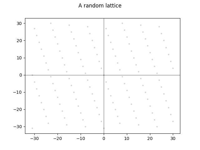
The points always follow a clear pattern that resembles “lattice work” you might see in a garden:

^{(Source: https://picryl.com/media/texture-wood-vintage-backgrounds-textures-8395bb)}

For cryptography, we care about a special class of lattices, those defined by a matrix P that “recognizes” points in the lattice. That is, the lattice recognized by P is the set of vectors v for which P*v == 0, where “0” denotes the all-zero vector. The all-zero vector is np.zeros((N,1), dtype=int) in NumPy.

Readers familiar with linear algebra may have a different definition of lattices in mind: in general, a lattice is the set of points obtained by taking linear combinations of some basis. Our lattices can also be formulated in this way, i.e., for a matrix P that recognizes a lattice, we can compute the basis vectors that generate the lattice. However, we don’t much care about this representation here.

The LWE problem boils down to distinguishing a set of points that are “close to” the lattice from a set of points that are “far away from” the lattice. We construct these points from an LWE instance and a random (A,t) respectively. Here we have an LWE sample (left) and a sample from the random distribution (right):

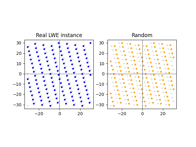
What this shows is that the points of the LWE instance are much closer to the lattice than the random instance. This is indeed the case on average. However, while distinguishing LWE instances from random is easy in two dimensions, it gets harder in higher dimensions.

Let’s take a look at how we construct these points. First, let’s take an LWE instance (A,t=(A*s + e) % Q) and consider the lattice recognized by the matrix P we get by concatenating A with the identity matrix I. This might look something like this (N=3):

A = gen_mat(N, N, 0, Q)
P = np.concatenate((A, np.identity(N, dtype=int)), axis=1)
print(P)
# [[1570  634  161	1	0	0]
#  [1522 1215  861	0	1	0]
#  [ 344 2651 1889	0	0	1]]

Notice that we can compute t by multiplying P by the vector we get by concatenating s and e (beta=2):

s = gen_mat(N, 1, -beta, beta+1)
e = gen_mat(N, 1, -beta, beta+1)
t = (A*s + e) % Q
z = np.concatenate((s, e))
print(z)
# [[-2]
#  [ 0]
#  [-2]
#  [ 0]
#  [-1]
#  [ 2]]
assert np.array_equal(t, P*z % Q)

Let z denote this vector and consider the set of points v for which P*v == t. By definition, we say this set of points is “close to” the lattice because z is a short vector. (Remember: by “short” we mean its entries are bounded around 0 by beta.)

Now consider a random (A,t) and consider the set of points v for which P*v == t. We won’t prove it, but it is a fact that this set of points is likely to be “far away from” the lattice in the sense that there is no short vector z for which P*z == t.

Intuitively, solving LWE gets harder as z gets longer. Indeed, increasing the average length of z (by making beta larger) increases the average distance to the lattice, making it look more like a random instance:

On the other hand, making z too long creates another problem.

Breaking lattice cryptography by finding short vectors

Given a random matrix A, the Short Integer Solution (SIS) problem is to find short vectors (i.e., whose entries are bounded by beta) z1 and z2 for which (A*z1 + z2) % Q is zero. Notice that this is equivalent to finding a short vector z in the lattice recognized by P:

z = np.concatenate((z1, z2))
assert np.array_equal((A*z1 + z2) % Q, P*z % Q)

If we had a (quantum) computer program for solving SIS, then we could use this program to solve LWE as well: if (A,t) is an LWE instance, then z1.T*t will be small; otherwise, if (A,t) is random, then z1.T*t will be uniformly random. (You can convince yourself of this using a little algebra.) Therefore, in order for our encryption scheme to be secure, it must be hard to find short vectors in the lattice defined by those parameters.

Intuitively, finding long vectors in the lattice is easier than finding short ones, which means that solving the SIS problem gets easier as beta gets closer to Q. On the other hand, as beta gets closer to 0, it gets easier to distinguish LWE instances from random!

This suggests a kind of Goldilocks zone for LWE-based encryption: if the secret and noise vectors are too short, then LWE is easy; but if the secret and noise vectors are too long, then SIS is easy. The optimal choice is somewhere in the middle.

Enough math, just give me my parameters!

To tune our encryption scheme, we want to choose parameters for which the most efficient known algorithms (quantum or classical) for solving LWE are out of reach for any attacker with as many resources as we can imagine (and then some, in case new algorithms are discovered). But how do we know which attacks to look out for?

Fortunately, the community of expert lattice cryptographers and cryptanalysts maintains a tool called lattice-estimator that estimates the complexity of the best known (quantum) algorithms for lattice problems relevant to cryptography. Here’s what we get when we run this tool for ML-KEM (this requires Sage to run):

sage: from estimator import *
sage: res = LWE.estimate.rough(schemes.Kyber768)
usvp        :: rop: ≈2^182.2, red: ≈2^182.2, δ: 1.002902, β: 624, d: 1427, tag: usvp
dual_hybrid :: rop: ≈2^174.3, red: ≈2^174.3, guess: ≈2^162.5, β: 597, p: 4, ζ: 10, t: 60, β': 597, N: ≈2^122.7, m: 768

The number that we’re most interested in is “rop“, which estimates the amount of computation the attack would consume. Playing with this tool a bit, we eventually find some parameters for our scheme for which the “usvp” and “dual_hybrid” attacks have comparable complexity. However, lattice-estimator identifies an attack it calls “arora-gb” that applies to our scheme, but not to ML-KEM, that has much lower complexity. (N=600, Q=3329, and beta=4):

sage: res = LWE.estimate.rough(LWE.Parameters(n=600, q=3329, Xs=ND.Uniform(-4,4), Xe=ND.Uniform(-4,4)))
usvp        :: rop: ≈2^180.2, red: ≈2^180.2, δ: 1.002926, β: 617, d: 1246, tag: usvp
dual_hybrid :: rop: ≈2^226.2, red: ≈2^225.4, guess: ≈2^224.9, β: 599, p: 3, ζ: 10, t: 0, β': 599, N: ≈2^174.8, m: 600
arora-gb    :: rop: ≈2^129.4, dreg: 9, mem: ≈2^129.4, t: 4, m: ≈2^64.7

We’d have to bump the parameters even further to the scheme to a regime that has comparable security to ML-KEM.

Finally, a word of warning: when designing lattice cryptography, determining whether our scheme is secure requires a lot more than estimating the cost of generic attacks on our LWE parameters. In the absence of a mathematical proof of security in a realistic adversarial model, we can’t rule out other ways of breaking our scheme. Tread lightly, fair traveler, and bring a friend along for the journey.

Making the scheme efficient

Now that we understand how to encrypt with LWE, let’s take a quick look at how to make our scheme efficient.

The main problem with our scheme is that we can only encrypt a bit at a time. This is because we had to split the range(Q) into two chunks, one that encodes 1 and another that encodes 0. We could improve the bit rate by splitting the range into more chunks, but this would make decryption errors more likely.

Another problem with our scheme is that the runtime depends heavily on our security parameters. Encryption requires O(N²) multiplications (multiplication is the most expensive part of a secure implementation of modular arithmetic), and in order for our scheme to be secure, we need to make N quite large.

ML-KEM solves both of these problems by replacing modular arithmetic with arithmetic over a polynomial ring. This means the entries of our matrices will be polynomials rather than integers. We need to define what it means to add, subtract, and multiply polynomials, but once we’ve done that, everything else about the encryption scheme is the same.

In fact, you probably learned polynomial arithmetic in grade school. The only thing you might not be familiar with is polynomial modular reduction. To multiply two polynomials $f(X)$ and $g(X)$, we start by multiplying $f(X)\cdot g(X)$ as usual. Then we’re going to divide $f(X)\cdot g(X)$ by some special polynomial — ML-KEM uses $X^{256}+1$ — and take the remainder. We won’t try to explain this algorithm, but the takeaway is that the result is a polynomial with $256$ coefficients, each of which is an integer in range(Q).

The main advantage of using a polynomial ring for arithmetic is that we can pack more bits into the ciphertext. Our formula for the ciphertext is exactly the same (u=r.T*A + e2, v=r.T*t + e3 + m), but this time the plaintext m encodes a polynomial. Each coefficient of the polynomial encodes a bit, and we’ll handle decryption errors just as we did before, by splitting range(Q) into two chunks, one that encodes 1 and another that encodes 0. This allows us to reliably encrypt 256 bits (32 bytes) per ciphertext.

Another advantage of using polynomials is that it significantly reduces the dimension of the matrix without impacting security. Concretely, the most widely used variant of ML-KEM, ML-KEM-768, uses a 3-by-3 matrix A, so just 9 polynomials in total. (Note that $256 \cdot 3 = 768$, hence the name “ML-KEM-768”.) However, note that we have to be careful in how we choose the modulus: $X^{256}+1$ is special in that it does not exhibit any algebraic structure that is known to permit attacks.

The choices of Q=3329 for the coefficient modulus and $X^{256}+1$ for the polynomial modulus have one more benefit. They allow polynomial multiplication to be carried out using the NTT algorithm, which massively reduces the number of multiplications and additions we have to perform. In fact, this optimization is a major reason why ML-KEM is sometimes faster in terms of CPU time than key exchange with elliptic curves.

We won’t get into how NTT works here, except to say that the algorithm will look familiar to you if you’ve ever implemented RSA. In both cases we use the Chinese Remainder Theorem to split multiplication up into multiple, cheaper multiplications with smaller moduli.

From public key encryption to ML-KEM

The last step to build ML-KEM is to make the scheme secure against chosen ciphertext attacks (CCA). Currently, it’s only secure against chosen plaintext attacks (CPA), which basically means that the ciphertext leaks no information about the plaintext, regardless of the distribution of plaintexts. CCA security is stronger in that it gives the attacker access to decryptions of ciphertexts of its choosing. (Of course, it’s not allowed to decrypt the target ciphertext itself.) The specific transform used in ML-KEM results in a CCA-secure KEM (“Key-Encapsulation Mechanism”).

Chosen ciphertext attacks might seem a bit abstract, but in fact they formalize a realistic threat model for many applications of KEMs (and public key encryption for that matter). For example, suppose we use the scheme in a protocol in which the server authenticates itself to a client by proving it was able to decrypt a ciphertext generated by the client. In this kind of protocol, the server acts as a sort of “decryption oracle” in which its responses to clients depend on the secret key. Unless the scheme is CCA secure, this oracle can be abused by an attacker to leak information about the secret key over time, allowing it to eventually impersonate the server.

ML-KEM incorporates several more optimizations to make it as fast and as compact as possible. For example, instead of generating a random matrix A, we can derive it from a random, 32-byte string (called a “seed”) using a hash-based primitive called a XOF (“eXtendable Output Function”), in the case of ML-KEM this XOF is SHAKE128. This significantly reduces the size of the public key.

Another interesting optimization is that the polynomial coefficients (integers in range(Q)) in the ciphertext are compressed by rounding off the least significant bits of each coefficient, thereby reducing the overall size of the ciphertext.

All told, for the most widely deployed parameters (ML-KEM-768), the public key is 1184 bytes and the ciphertext is 1088 bytes. There’s no obvious way to reduce this, except by reducing the size of the encapsulated key or the size of the public matrix A. The former would make ML-KEM useful for fewer applications, and the latter would reduce the security margin.

Note that there are other lattice schemes that are smaller, but they are based on different hardness assumptions and are still undergoing analysis.

Authentication

In the previous section, we learned about ML-KEM, the algorithm already in use to make encryption PQ-secure. However, encryption is only one piece of the puzzle: establishing a secure connection also requires authenticating the server — and sometimes the client, depending on the application.

Authentication is usually provided by a digital signature scheme, which uses a secret key to sign a message and a public key to verify the signature. The signature schemes used today aren’t PQ-secure: a quantum computer can be used to compute the secret key corresponding to a server’s public key, then use this key to impersonate the server.

While this threat is less urgent than the threat to encryption, mitigating it is going to be more complicated. Over the years, we’ve bolted a number of signatures onto the TLS handshake in order to meet the evolving requirements of the web PKI. We have PQ alternatives for these signatures, one of which we’ll study in this section, but so far these signatures and their public keys are too large (i.e., take up too many bytes) to make comfortable replacements for today’s schemes. Barring some breakthrough in NIST’s ongoing standardization effort, we will have to re-engineer TLS and the web PKI to use fewer signatures.

For now, let’s dive into the PQ signature scheme we’re likely to see deployed first: ML-DSA, a.k.a. Dillithium. The design of ML-DSA follows a similar template as ML-KEM. We start by building some intermediate primitive, then we transform that primitive into the primitive we want, in this case a signature scheme.

ML-DSA is quite a bit more involved than ML-KEM, so we’re going to try to boil it down even further and just try to get across the main ideas.

Warm up

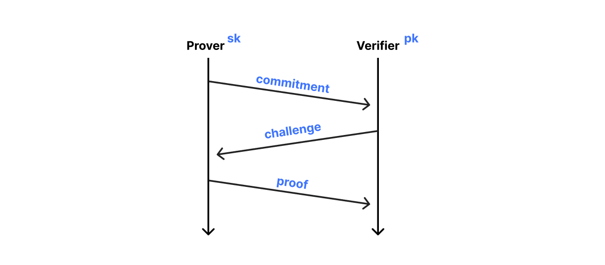
Whereas ML-KEM is basically El Gamal encryption with elliptic curves replaced with lattices, ML-DSA is basically the Schnorr identification protocol with elliptic curves replaced with lattices. Schnorr’s protocol is used by a prover to convince a verifier that it knows the secret key associated with its public key without revealing the secret key itself. The protocol has three moves and is executed with four algorithms:

initialize(): The prover initializes the protocol and sends a commitment to the verifier
challenge(): The verifier receives the commitment and sends the prover a challenge
finish(): The prover receives the challenge and sends the verifier the proof
verify(): Finally, the verifier uses the proof to decide whether the prover knows the secret key

We get the high-level structure of ML-DSA by making this protocol non-interactive. In particular, the prover derives the challenge itself by hashing the commitment together with the message to be signed. The signature consists of the commitment and proof: to verify the signature, the verifier recomputes the challenge from the commitment and message and runs verify()as usual.

Let’s jump right in to building Schnorr’s identification protocol from lattices. If you’ve never seen this protocol before, then this will look a little like black magic at first. We’ll go through it slowly enough to see how and why it works.

Just like for ML-KEM, our public key is an LWE instance (A,t=A*s1 + s2). However, this time our secret key is the pair of short vectors (s1,s2), i.e., it includes the error term. Otherwise, key generation is exactly the same:

def key_gen():
    A = gen_mat(N, N, 0, Q)
    s1 = gen_mat(N, 1, -beta, beta+1)
    s2 = gen_mat(N, 1, -beta, beta+1)
    t = (A*s1 + s2) % Q
    return ((A, t), (s1, s2))

To initialize the protocol, the prover generates another LWE instance (A,w=A*y1 + y2). You’ll see why in just a moment. The prover sends the hash of w as its commitment:

def initialize(A):
    y1 = gen_mat(N, 1, -beta, beta+1)
    y2 = gen_mat(N, 1, -beta, beta+1)
    w = (A*y1 + y2) % Q
    return (H(w), (y1, y2))

Here H is some cryptographic hash function, like SHA-3. The prover stores the secret vectors (y1,y2) for use in its next move.

Now it’s time for the verifier’s challenge. The challenge is just an integer, but we need to be careful about how we choose it. For now let’s just pick it at random:

def challenge():
    return random.randrange(0, Q)

Remember: when we turn this protocol into a digital signature, the challenge is derived from the commitment, H(w), and the message. The range of this hash function must be the same as the set of outputs of challenge().

Now comes the fun part. The proof is a pair of vectors (z1,z2) satisfying A*z1 + z2 == c*t + w. We can easily produce this proof if we know the secret key:

z1 = (c*s1 + y1) % Q

z2 = (c*s2 + y2) % Q

Then A*z1 + z2 == A*(c*s1 + y1) + (c*s2 + y2) == c*(A*s1 + s2) + (A*y1 + y2) == c*t + w. Our goal is to design the protocol such that it’s hard to come up with (z1,z2) without knowing (s1,s2), even after observing many executions of the protocol.

Here are the finish() and verify() algorithms for completeness:

def finish(s1, s2, y1, y2, c):
    z1 = (c*s1 + y1) % Q
    z2 = (c*s2 + y2) % Q
    return (z1, z2)

def verify(A, t, hw, c, z1, z2):
	return H((A*z1 + z2 - c*t) % Q) == hw

# Test
((A, t), (s1, s2)) = key_gen()
(hw, (y1, y2)) = initialize(A)        # hw: prover -> verifier
c = challenge()                       # c: verifier -> prover
(z1, z2) = finish(s1, s2, y1, y2, c)  # (z1, z2): prover -> verifier
assert verify(A, t, hw, c, z1, z2)    # verifier

Notice that the verifier doesn’t actually check A*z1 + z2 == c*t + w directly; we have to rearrange the equation so that we can set the commitment to H(w) rather than w. We’ll explain the need for hashing in the next section.

Making this scheme secure

The question of whether this protocol is secure boils down to whether it’s possible to impersonate the prover without knowledge of the secret key. Let’s put our attacker hat on and poke around.

Perhaps there’s a way to compute the secret key, either from the public key directly or by eavesdropping on executions of the protocol with the honest prover. If LWE is hard, then clearly there’s no way we’re going to extract the secret key from the public key t. Likewise, the commitment H(w)doesn’t leak any information that would help us extract the secret key from the proof (z1,z2).

Let’s take a closer look at the proof. Notice that the vectors (y1,y2) “mask” the secret key vectors, sort of how the shared secret masks the plaintext in ML-KEM. However, there’s one big exception: we also scale the secret key vectors by the challenge c.

What’s the effect of scaling these vectors? If we squint at a few proofs, we start to see a pattern emerge. Let’s look at z1 first (N=3, Q=3329, beta=4):

((A, t), (s1, s2)) = key_gen()
print('s1={}'.format(s1.T % Q))
for _ in range(10):
    (w, (y1, y2)) = initialize(A)
    c = challenge()
    (z1, z2) = finish(s1, s2, y1, y2, c)
    print('c={}, z1={}'.format(c, z1.T))
# s1=[[   1	0 3326]]
# c=1123, z1=[[1121 3327 3287]]
# c=1064, z1=[[1060	4  137]]
# c=1885, z1=[[1884 3327  999]]
# c=269, z1=[[ 270 3325 2524]]
# c=1506, z1=[[1510 3325 2141]]
# c=3147, z1=[[3149	4  547]]
# c=703, z1=[[ 700	4 1219]]
# c=1518, z1=[[1518 3327 2104]]
# c=1726, z1=[[1726	0 1478]]
# c=2591, z1=[[2589	4 2217]]

Indeed, with enough proof samples, we should be able to make a pretty good guess of the value of s1. In fact, for these parameters, there is a simple statistical analysis we can do to compute s1 exactly. (Hint: Q is a prime number, which means c*pow(c,-1,Q)==1 whenever c>0.) We can also apply this analysis to s2, or compute it directly from t, s1, and A.

The main flaw in our protocol is that, although our secret vectors are short, scaling them makes them so long that they’re not completely masked by (y1,y2). Since c spans the entire range(Q), so do the entries of c*s1. and c*s2, which means in order to mask these entries, we need the entries of (y1,y2) to span range(Q) as well. However, doing this would make solving LWE for (A,w) easy, by solving SIS. We somehow need to strike a balance between the length of the vectors of our LWE instances and the leakage induced by the challenge.

Here’s where things get tricky. Let’s refer to the set of possible outputs of challenge() as the challenge space. We need the challenge space to be fairly large, large enough that the probability of outputting the same challenge twice is negligible.

Why would such a collision be a problem? It’s a little easier to see in the context of digital signatures. Let’s say an attacker knows a valid signature for a message m. The signature includes the commitment H(m), so the attacker also knows the challenge is c == H(H(w),m). Suppose it manages to find a different message m^* for which c == H(H(w),m^*). Then the signature is also valid for m! And this attack is easy to pull off if the challenge space, that is, the set of possible outputs of H, is too small.

Unfortunately, we can’t make the challenge space larger simply by increasing the size of the modulus Q: the larger the challenge might be, the more information we’d leak about the secret key. We need a new idea.

The best of both worlds

Remember that the hardness of LWE depends on the ratio between beta and Q. This means that y1 and y2 don’t need to be short in absolute terms, but short relative to random vectors.

With that in mind, consider the following idea. Let’s take a larger modulus, say Q=2**31 - 1, and we’ll continue to sample from the same challenge space, range(2**16).

First, notice that z1 is now “relatively” short, since its entries are now in range(-gamma, gamma+1), where gamma = beta*(2**16-1), rather than uniform over range(Q). Let’s also modify initialize() to sample the entries of (y1,y2) from the same range and see what happens:

def initialize(A):
	y1 = gen_mat(N, 1, -gamma, gamma+1)
	y2 = gen_mat(N, 1, -gamma, gamma+1)
	w = (A*y1 + y2) % Q
	return (H(w), (y1, y2))

((A, t), (s1, s2)) = key_gen()
print('s1={}'.format(s1.T % Q))
for _ in range(10):
    (w, (y1, y2)) = initialize(A)
    c = challenge()
    (z1, z2) = finish(s1, s2, y1, y2, c)
    print('c={}, z1={}'.format(c, z1.T))
# s1=[[3 0 1]]
# c=31476, z1=[[175933 141954  93186]]
# c=27360, z1=[[    136404 2147438807     283758]]
# c=33536, z1=[[2147430945 2147377022     190671]]
# c=23283, z1=[[186516  73400   4955]]
# c=24756, z1=[[    328377 2147438906 2147388768]]
# c=12428, z1=[[2147340715     188675      90282]]
# c=24266, z1=[[    175498 2147261581 2147301553]]
# c=45331, z1=[[357595 185269 177155]]
# c=45641, z1=[[     21592 2147249191 2147446200]]
# c=57893, z1=[[297750 113335 144894]]

This is definitely going in the right direction, since there are no obvious correlations between z1 and s1. (Likewise for z2 and s2.) However, we’re not quite there.

One problem is that the challenge space is still quite small. With only 2**16 challenges to choose from, we’re likely to see a collision even after only a handful of protocol executions. We need the challenge space to be much, much larger, say around 2**256. But then Q has to be an insanely large number in order for the beta to Q ratio to be secure.

ML-DSA is able to side step this problem due to its use of arithmetic over polynomial rings. It uses the same modulus polynomial as ML-KEM, so the challenge is a polynomial with 256 coefficients. The coefficients are chosen carefully so that the challenge space is large, but multiplication by the challenge scales the secret vector by a small amount. Note that we still end up using a slightly larger modulus (Q=8380417) for ML-DSA than for ML-KEM, but only by about twelve bits.

However, there is a more fundamental problem here, which is that we haven’t completely ruled out that signatures may leak information about the secret key.

Cause and effect

Suppose we run the protocol a number of times, and in each run, we happen to choose a relatively small value for some entry of y1. After enough runs, this would eventually allow us to reconstruct the corresponding entry of s1. To rule this out as a possibility, we need to make y1 even longer. (Likewise for y2.) But how long?

Suppose we know that the entries of z1 and z2 are always in range(-beta_loose,beta_loose+1) for some beta_loose > beta. Then we can simulate an honest run of the protocol as follows:

def simulate(A, t):
    z1 = gen_mat(N, 1, -beta_loose, beta_loose+1)
    z2 = gen_mat(N, 1, -beta_loose, beta_loose+1)
    c = challenge()
    w = (A*z1 + z2 - c*t) % Q
    return (H(w), c, (z1, z2))

# Test
((A, t), (s1, s2)) = key_gen()
(hw, c, (z1, z2)) = simulate(A, t)
assert verify(A, t, hw, c, z1, z2)

This procedure perfectly simulates honest runs of the protocol, in the sense that the output of simulate() is indistinguishable from the transcript of a real run of the protocol with the honest prover. To see this, notice that the w, c, z1, and z2 all have the same mathematical relationship (the verification equation still holds) and have the same distribution.

And here’s the punch line: since this procedure doesn’t use the secret key, it follows that the attacker learns nothing from eavesdropping on the honest prover that it can’t compute from the public key itself. Pretty neat!

What’s left to do is arrange for z1 and z2 to fall in this range. First, we modify initialize() by increasing the range of y1 and y2 by beta_loose:

def initialize(A):
    y1 = gen_mat(N, 1, -gamma+beta_loose, gamma+beta_loose+1)
    y2 = gen_mat(N, 1, -gamma+beta_loose, gamma+beta_loose+1)
    w = (A*y1 + y2) % Q
    return (H(w), (y1, y2))

This ensures the proof vectors z1 and z2 are roughly uniform over range(-beta_loose, beta_loose+1). However, they may fall slightly outside of this range, so need to modify finalize() to abort if not. Correspondingly, verify() should reject proof vectors that are out of range:

def finish(s1, s2, y1, y2, c):
    z1 = (c*s1 + y1) % Q
    z2 = (c*s2 + y2) % Q
    if not in_range(z1, beta_loose) or not in_range(z2, beta_loose):
        return (None, None)
    return (z1, z2)

def verify(A, t, hw, c, z1, z2):
    if not in_range(z1, beta_loose) or not in_range(z2, beta_loose):
        return False
    return H((A*z1 + z2 - c*t) % Q) == hw

If finish() returns (None,None), then the prover and verifier are meant to abort the protocol and retry until the protocol succeeds:

((A, t), (s1, s2)) = key_gen()
while True:
    (hw, (y1, y2)) = initialize(A)        # hw: prover -> verifier
    c = challenge()                       # c: verifier -> prover
    (z1, z2) = finish(s1, s2, y1, y2, c)  # (z1, z2): prover -> verifier
    if z1 is not None and z2 is not None:
        break
assert verify(A, t, hw, c, z1, z2)

Interestingly, we should expect aborts to be quite common. The parameters of ML-DSA are tuned so that the protocol runs five times on average before it succeeds.

Another interesting point is that the security proof requires us to simulate not only successful protocol runs, but aborted protocol runs as well. More specifically, the protocol simulator must abort with the same probability as the real protocol, which implies that the rejection probability is independent of the secret key.

The simulator also needs to be able to produce realistic looking commitments for aborted transcripts. This is exactly why the prover commits to the hash of w rather than w itself: in the security proof, we can easily simulate hashes of random inputs.

Making this scheme efficient

ML-DSA benefits from many of the same optimizations as ML-KEM, including using polynomial rings, NTT for polynomial multiplication, and encoding polynomials with a fixed number of bits. However, ML-DSA has a few more tricks to make things smaller.

First, in ML-DSA, instead of the pair of short vectors z1 and z2, the proof consists of a single vector z=c*s1 + y, where y was committed to in the previous step. In turn, we only end up with a single proof vector z rather than two as before. Getting this to work requires a special encoding of the commitment so that we can’t compute y from it. ML-DSA uses a related trick to reduce the size of the t vector of the public key, but the details are more complicated.

For the parameters we expect to deploy first (ML-DSA-44), the public key is 1312 bytes long and the signature is a whopping 2420 bytes. In contrast to ML-KEM, it is possible to shave off some more bytes. This does not come for free and requires complicating the scheme. An example is HAETAE, which changes the distributions used. Falcon takes it a step further with even smaller signatures, using a completely different approach, which although elegant is also more complex to implement.

Wrap up

Lattice cryptography underpins the first generation of PQ algorithms to get widely deployed on the Internet. ML-KEM is already widely used today to protect encryption from quantum computers, and in the coming years we expect to see ML-DSA deployed to get ahead of the threat of quantum computers to authentication.

Lattices are also the basis of a new frontier for cryptography: computing on encrypted data.

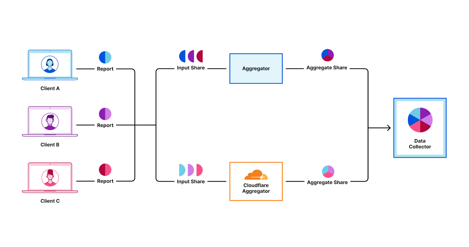
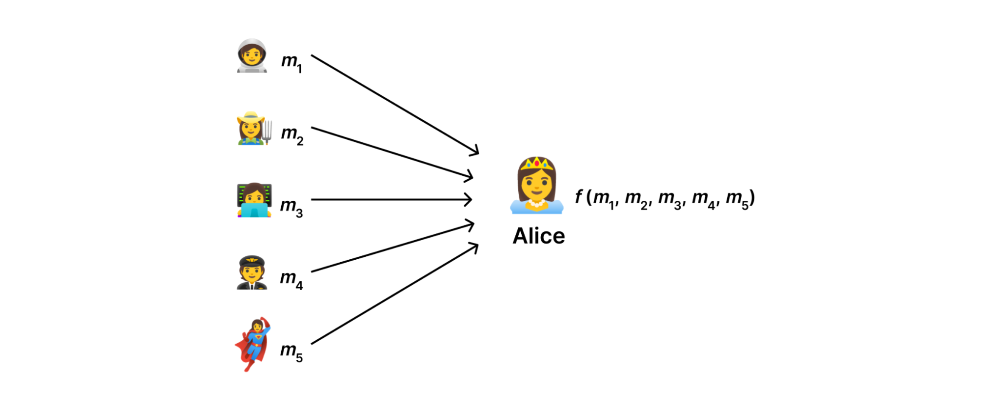
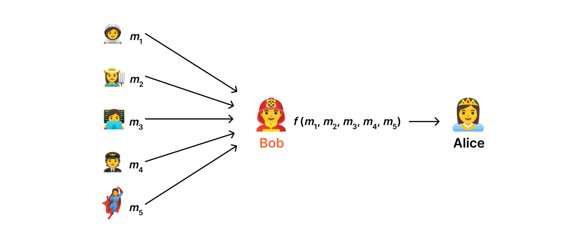
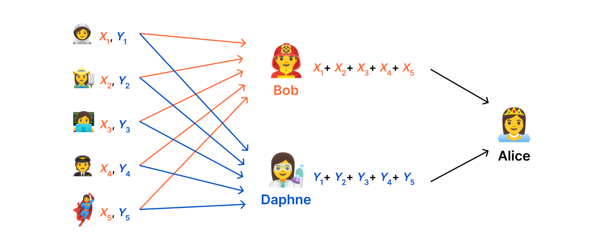
Suppose you wanted to aggregate some metrics submitted by clients without learning the metrics themselves. With LWE-based encryption, you can arrange for each client to encrypt their metrics before submission, aggregate the ciphertexts, then decrypt to get the aggregate.

Suppose instead that a server has a database that it wants to provide clients access to without revealing to the server which rows of the database the client wants to query. LWE-based encryption allows the database to be encoded in a manner that permits encrypted queries.

These applications are special cases of a paradigm known as FHE (“Fully Homomorphic Encryption”), which allows for arbitrary computations on encrypted data. FHE is an extremely powerful primitive, and the only way we know how to build it today is with lattices. However, for most applications, FHE is far less practical than a special-purpose protocol would be (lattice-based or not). Still, over the years we’ve seen FHE get better and better, and for many applications it is already a decent option. Perhaps we’ll dig into this and other lattice schemes in a future blog post.

We hope you enjoyed this whirlwind tour of lattices. Thanks for reading!

Privacy-preserving measurement and machine learning

2023-09-29 Christopher Patton

Post Syndicated from Christopher Patton original http://blog.cloudflare.com/deep-dive-privacy-preserving-measurement/

Privacy-preserving measurement and machine learning

In 2023, data-driven approaches to making decisions are the norm. We use data for everything from analyzing x-rays to translating thousands of languages to directing autonomous cars. However, when it comes to building these systems, the conventional approach has been to collect as much data as possible, and worry about privacy as an afterthought.

The problem is, data can be sensitive and used to identify individuals – even when explicit identifiers are removed or noise is added.

Cloudflare Research has been interested in exploring different approaches to this question: is there a truly private way to perform data collection, especially for some of the most sensitive (but incredibly useful!) technology?

Some of the use cases we’re thinking about include: training federated machine learning models for predictive keyboards without collecting every user’s keystrokes; performing a census without storing data about individuals’ responses; providing healthcare authorities with data about COVID-19 exposures without tracking peoples’ locations en masse; figuring out the most common errors browsers are experiencing without reporting which websites are visiting.

It’s with those use cases in mind that we’ve been participating in the Privacy Preserving Measurement working group at the IETF whose goal is to develop systems for collecting and using this data while minimizing the amount of per-user information exposed to the data collector.

So far, the most promising standard in this space is DAP – Distributed Aggregation Protocol – a clever way to use multi-party computation to aggregate data without exposing individual measurements. Early versions of the algorithms used by DAP have been implemented by Google and Apple for exposure notifications.

In this blog post, we’ll do a deep dive into the fundamental concepts behind the DAP protocol and give an example of how we’ve implemented it into Daphne, our open source aggregator server. We hope this will inspire others to collaborate with us and get involved in this space!

The principles behind DAP, an open standard for privacy preserving measurement

At a high level, using the DAP protocol forces us to think in terms of data minimization: collect only the data that we use and nothing more. Abstractly, our goal is to devise a system with which a data collector can compute some function $ f(m_{1},…,m_{N}) $ of measurements $ m_{1},…,m_{N} $ uploaded by users without observing the measurements in the clear.

This may at first seem like an impossible task: to compute on data without knowing the data we're computing on. Nevertheless, —and, as is often the case in cryptography— once we've properly constrained the problem, solutions begin to emerge.

In an ideal world (see above), there would be some server somewhere on the Internet that we could trust to consume measurements, aggregate them, and send the result to the data collector without ever disclosing anything else. However, in reality there's no reason for users to trust such a server more than the data collector; Indeed, both are subject to the usual assortment of attacks that can lead to a data breach.

Instead, what we do in DAP is distribute the computation across the servers such that no single server has a complete measurement. The key idea that makes this possible is secret sharing.

Computing on secret shared data

To set things up, let's make the problem a little more concrete. Suppose each measurement $ m_{i} $ is a number and our goal is to compute the sum of the measurements. That is, $ f(m_{1},…,m_{N}) = m_{1} + \cdots + m_{N} $. Our goal is to use secret sharing to allow two servers, which we'll call aggregators, to jointly compute this sum.

To understand secret sharing, we're going to need a tiny bit of math—modular arithmetic. The expression $ X + 1 (\textrm{mod}) \textit{q} $ means "add $ X $ and $ Y $, then divide the sum by $ q $ and return the remainder". For now the modulus $ q $ can be any large number, as long as it's larger than any sum we'd ever want to compute ($ 2 ^{64} $, say). In the remainder of this section, we'll omit $ q $ and simply write $ X + Y $ for addition modulo $ q $.

The goal of secret sharing is to shard a measurement (i.e., a "secret") into two "shares" such that (i) the measurement can be recovered by combining the shares together and (ii) neither share leaks any information about the measurement. To secret share each $ m_{i} $, we choose a random number $ R_{i} \in \lbrace 0,…,q – 1\rbrace $, set the first share to be $X_{i} = m_{i} – R_{i} $ and set the other share to be $ Y_{i} = R_{i} $. To recover the measurement, we simply add the shares together. This works because $ X_{i} + Y_{i} = (m_{i} – R_{i}) + R_{i} = m_{i} $. Moreover, each share is indistinguishable from a random number: For example, $ 1337 $ might be secret-shared into $ 11419752798245067454 $ and $ 7026991275464485499 $ (modulo $ q = 2^{64} $).

With this scheme we can devise a simple protocol for securely computing the sum:

Each client shards its measurement $ m_{i} $ into $ X_{i} $ and $ Y_{i} $ and sends one share to each server.
The first aggregator computes $ X = X_{1} + \cdots + X_{N} $ and reveals $ X $ to the data collector. The second aggregator computes $ Y = Y_{1} + \cdots + Y_{N} $ and reveals $ Y $ to the data collector.
The data collector unshards the result as $ r = X + Y $.

This works because the secret shares are additive, and the order in which we add things up is irrelevant to the function we're computing:

$ r = m_{1} + \cdots + m_{N} $ // by definition
$ r = (m_{1} – R_{1}) + R_{1} + \cdots (m_{N} – R_{N}) + R_{N} $ // apply sharding
$ r = (m_{1} – R_{1}) + \cdots + (m_{N} – R_{N}) + R_{1} + \cdots R_{N} $ // rearrange the sum
$ r = X + Y $ // apply aggregation

Rich data types

This basic template for secure aggregation was described in a paper from Henry Corrigan-Gibbs and Dan Boneh called "Prio: Private, Robust, and Scalable Computation of Aggregate Statistics" (NSDI 2017). This paper is a critical milestone in DAP's history, as it showed that a wide variety of aggregation tasks (not just sums) can be solved within one, simple protocol framework, Prio. With DAP, our goal in large part is to bring this framework to life.

All Prio tasks are instances of the same template. Measurements are encoded in a form that allows the aggregation function to be expressed as the sum of (shares of) the encoded measurements. For example:

To get arithmetic mean, we just divide the sum by the number of measurements.
Variance and standard deviation can be expressed as a linear function of the sum and the sum of squares (i.e., $ m_{i}, m_{i}^{2} $ for each $ i $).
Quantiles (e.g., median) can be estimated reasonably well by mapping the measurements into buckets and aggregating the histogram.
Linear regression (i.e., finding a line of best fit through a set of data points) is a bit more complicated, but can also be expressed in the Prio framework.

This degree of flexibility is essential for wide-spread adoption because it allows us to get the most value we can out of a relatively small amount of software. However, there are a couple problems we still need to overcome, both of which entail the need for some form of interaction.

Input validation

The first problem is input validation. Software engineers, especially those of us who operate web services, know in our bones that validating inputs we get from clients is of paramount importance. (Never, ever stick a raw input you got from a client into an SQL query!) But if the inputs are secret shared, then there is no way for an aggregator to discern even a single bit of the measurement, let alone check that it has an expected value. (A secret share of a valid measurement and a number sampled randomly from $ \lbrace 0,…,q – 1 \rbrace $ look identical.) At least, not on its own.

The solution adopted by Prio (and the standard, with some improvements), is a special kind of zero-knowledge proof (ZKP) system designed to operate on secret shared data. The goal is for a prover to convince a verifier that a statement about some data it has committed to is true (e.g., the user has a valid hardware key), without revealing the data itself (e.g. which hardware key is in-use).

Our setting is exactly the same, except that we're working on secret-shared data rather than committed data. Along with the measurement shares, the client sends shares of a validity proof; then during aggregation, the aggregators interact with one another in order to check and verify the proof. (One round-trip over the network is required.)

A happy consequence of working with secret shared data is that proof generation and verification are much faster than for committed (or encrypted) data. This is mainly because we avoid the use of public-key cryptography (i.e., elliptic curves) and are less constrained in how we choose cryptographic parameters. (We require the modulus $ q $ to be a prime number with a particular structure, but such primes are not hard to find.)

Non-linear aggregation

There are a variety of aggregation tasks for which Prio is not well-suited, in particular those that are non-linear. One such task is to find the "heavy hitters" among the set of measurements. The heavy hitters are the subset of the measurements that occur most frequently, say at least $ t $ times for some threshold $ t $. For example, the measurements might be the URLs visited on a given day by users of a web browser; the heavy hitters would be the set of URLs that were visited by at least $ t $ users.

This computation can be expressed as a simple program:

def heavy_hitters(measurements: list[bytes], t: int) -> set[bytes]:
    hh = defaultdict(lambda: 0)
    for measurement in measurements:
        hh[measurement] += 1
    return set(map(lambda x: x[0], filter(lambda x: x[1] >= t, hh.items())))

However, it cannot be expressed as a linear function, at least not efficiently (with sub-exponential space). This would be required to perform this computation on secret-shared measurements.

In order to enable non-linear computation on secret shared data, it is necessary to introduce some form of interaction. There are a few possibilities. For the heavy hitters problem in particular, Henry Corrigan-Gibbs and others devised a protocol called Poplar (IEEE Security & Privacy 2021) in which several rounds of aggregation and unsharding are performed, where in each round, information provided by the collector is used to "query" the measurements to obtain a refined aggregate result.

Helping to build a world of multi-party computation

Protocols like Prio or Poplar that enable computation over secret shared data fit into a rich tradition in cryptography known as multi-party computation (MPC). MPC is at once an active research area in theoretical computer science and a class of protocols that are beginning to see real-world use—in our case, to minimize the amount of privacy-sensitive information we collect in order to keep the Internet moving.

The PPM working group at IETF represents a significant effort, by Cloudflare and others, to standardize MPC techniques for privacy preserving measurement. This work has three main prongs:

To identify the types of problems that need to be solved.
To provide cryptography researchers from academia, industry, and the public sector with "templates" for solutions that we know how to deploy. One such template is called a "Verifiable Distributed Aggregation Function (VDAF)", which specifies a kind of "API boundary" between protocols like Prio and Poplar and the systems that are built around them. Cloudflare Research is leading development of the standard, contributing to implementations, and providing security analysis.
To provide a deployment roadmap for emerging protocols. DAP is one such roadmap: it specifies execution of a generic VDAF over HTTPS and attends to the various operational considerations that arise as deployments progress. As well as contributing to the standard itself, Cloudflare has developed its own implementation designed for our own infrastructure (see below).

The IETF is working on its first set of drafts (DAP/VDAF). These drafts are mature enough to deploy, and a number of deployments are scaling up as we speak. Our hope is that we have initiated positive feedback between theorists and practitioners: as new cryptographic techniques emerge, more practitioners will begin to work with them, which will lead to identifying new problems to solve, leading to new techniques, and so on.

Daphne: Cloudflare’s implementation of a DAP Aggregation Server

Our emerging technology group has been working on Daphne, our Rust-based implementation of a DAP aggregator server. This is only half of a deployment – DAP architecture requires two aggregator servers to interoperate, both operated by different parties. Our current version only implements the DAP Helper role; the other role is the DAP Leader. Plans are in the works to implement the Leader as well, which will open us up to deploy Daphne for more use cases.

We made two big decisions in our implementation here: using Rust and using Workers. Rust has been skyrocketing in popularity in the past few years due to its performance and memory management – a favorite of cryptographers for similar reasons. Workers is Cloudflare’s serverless execution environment that allows developers to easily deploy applications globally across our network – making it a favorite tool to prototype with at Cloudflare. This allows for easy integration with our Workers-based storage solutions like: Durable Objects, which we’re using for storing various data artifacts as required by the DAP protocol; and KV, which we’re using for managing aggregation task configuration. We’ve learned a lot from our interop tests and deployment, which has helped improve our own Workers products and which we have also fed back into the PPM working group to help improve the DAP standard.

If you’re interested in learning more about Daphne or collaborating with us in this space, you can fill out this form. If you’d like to get involved in the DAP standard, you can check out the working group.

Good-bye ESNI, hello ECH!

2020-12-08 Christopher Patton

Post Syndicated from Christopher Patton original https://blog.cloudflare.com/encrypted-client-hello/

Good-bye ESNI, hello ECH!

Most communication on the modern Internet is encrypted to ensure that its content is intelligible only to the endpoints, i.e., client and server. Encryption, however, requires a key and so the endpoints must agree on an encryption key without revealing the key to would-be attackers. The most widely used cryptographic protocol for this task, called key exchange, is the Transport Layer Security (TLS) handshake.

In this post we’ll dive into Encrypted Client Hello (ECH), a new extension for TLS that promises to significantly enhance the privacy of this critical Internet protocol. Today, a number of privacy-sensitive parameters of the TLS connection are negotiated in the clear. This leaves a trove of metadata available to network observers, including the endpoints’ identities, how they use the connection, and so on.

ECH encrypts the full handshake so that this metadata is kept secret. Crucially, this closes a long-standing privacy leak by protecting the Server Name Indication (SNI) from eavesdroppers on the network. Encrypting the SNI secret is important because it is the clearest signal of which server a given client is communicating with. However, and perhaps more significantly, ECH also lays the groundwork for adding future security features and performance enhancements to TLS while minimizing their impact on the privacy of end users.

ECH is the product of close collaboration, facilitated by the IETF, between academics and the tech industry leaders, including Cloudflare, our friends at Fastly and Mozilla (both of whom are the affiliations of co-authors of the standard), and many others. This feature represents a significant upgrade to the TLS protocol, one that builds on bleeding edge technologies, like DNS-over-HTTPS, that are only now coming into their own. As such, the protocol is not yet ready for Internet-scale deployment. This article is intended as a sign post on the road to full handshake encryption.

Background

The story of TLS is the story of the Internet. As our reliance on the Internet has grown, so the protocol has evolved to address ever-changing operational requirements, use cases, and threat models. The client and server don’t just exchange a key: they negotiate a wide variety of features and parameters: the exact method of key exchange; the encryption algorithm; who is authenticated and how; which application layer protocol to use after the handshake; and much, much more. All of these parameters impact the security properties of the communication channel in one way or another.

SNI is a prime example of a parameter that impacts the channel’s security. The SNI extension is used by the client to indicate to the server the website it wants to reach. This is essential for the modern Internet, as it’s common nowadays for many origin servers to sit behind a single TLS operator. In this setting, the operator uses the SNI to determine who will authenticate the connection: without it, there would be no way of knowing which TLS certificate to present to the client. The problem is that SNI leaks to the network the identity of the origin server the client wants to connect to, potentially allowing eavesdroppers to infer a lot of information about their communication. (Of course, there are other ways for a network observer to identify the origin — the origin’s IP address, for example. But co-locating with other origins on the same IP address makes it much harder to use this metric to determine the origin than it is to simply inspect the SNI.)

Although protecting SNI is the impetus for ECH, it is by no means the only privacy-sensitive handshake parameter that the client and server negotiate. Another is the ALPN extension, which is used to decide which application-layer protocol to use once the TLS connection is established. The client sends the list of applications it supports — whether it’s HTTPS, email, instant messaging, or the myriad other applications that use TLS for transport security — and the server selects one from this list, and sends its selection to the client. By doing so, the client and server leak to the network a clear signal of their capabilities and what the connection might be used for.

Some features are so privacy-sensitive that their inclusion in the handshake is a non-starter. One idea that has been floated is to replace the key exchange at the heart of TLS with password-authenticated key-exchange (PAKE). This would allow password-based authentication to be used alongside (or in lieu of) certificate-based authentication, making TLS more robust and suitable for a wider range of applications. The privacy issue here is analogous to SNI: servers typically associate a unique identifier to each client (e.g., a username or email address) that is used to retrieve the client’s credentials; and the client must, somehow, convey this identity to the server during the course of the handshake. If sent in the clear, then this personally identifiable information would be easily accessible to any network observer.

A necessary ingredient for addressing all of these privacy leaks is handshake encryption, i.e., the encryption of handshake messages in addition to application data. Sounds simple enough, but this solution presents another problem: how do the client and server pick an encryption key if, after all, the handshake is itself a means of exchanging a key? Some parameters must be sent in the clear, of course, so the goal of ECH is to encrypt all handshake parameters except those that are essential to completing the key exchange.

In order to understand ECH and the design decisions underpinning it, it helps to understand a little bit about the history of handshake encryption in TLS.

Handshake encryption in TLS

TLS had no handshake encryption at all prior to the latest version, TLS 1.3. In the wake of the Snowden revelations in 2013, the IETF community began to consider ways of countering the threat that mass surveillance posed to the open Internet. When the process of standardizing TLS 1.3 began in 2014, one of its design goals was to encrypt as much of the handshake as possible. Unfortunately, the final standard falls short of full handshake encryption, and several parameters, including SNI, are still sent in the clear. Let’s take a closer look to see why.

The TLS 1.3 protocol flow is illustrated in Figure 1. Handshake encryption begins as soon as the client and server compute a fresh shared secret. To do this, the client sends a key share in its ClientHello message, and the server responds in its ServerHello with its own key share. Having exchanged these shares, the client and server can derive a shared secret. Each subsequent handshake message is encrypted using the handshake traffic key derived from the shared secret. Application data is encrypted using a different key, called the application traffic key, which is also derived from the shared secret. These derived keys have different security properties: to emphasize this, they are illustrated with different colors.

The first handshake message that is encrypted is the server’s EncryptedExtensions. The purpose of this message is to protect the server’s sensitive handshake parameters, including the server’s ALPN extension, which contains the application selected from the client’s ALPN list. Key-exchange parameters are sent unencrypted in the ClientHello and ServerHello.

All of the client’s handshake parameters, sensitive or not, are sent in the ClientHello. Looking at Figure 1, you might be able to think of ways of reworking the handshake so that some of them can be encrypted, perhaps at the cost of additional latency (i.e., more round trips over the network). However, extensions like SNI create a kind of “chicken-and-egg” problem.

The client doesn’t encrypt anything until it has verified the server’s identity (this is the job of the Certificate and CertificateVerify messages) and the server has confirmed that it knows the shared secret (the job of the Finished message). These measures ensure the key exchange is authenticated, thereby preventing monster-in-the-middle (MITM) attacks in which the adversary impersonates the server to the client in a way that allows it to decrypt messages sent by the client. Because SNI is needed by the server to select the certificate, it needs to be transmitted before the key exchange is authenticated.

In general, ensuring confidentiality of handshake parameters used for authentication is only possible if the client and server already share an encryption key. But where might this key come from?

Full handshake encryption in the early days of TLS 1.3. Interestingly, full handshake encryption was once proposed as a core feature of TLS 1.3. In early versions of the protocol (draft-10, circa 2015), the server would offer the client a long-lived public key during the handshake, which the client would use for encryption in subsequent handshakes. (This design came from a protocol called OPTLS, which in turn was borrowed from the original QUIC proposal.) Called “0-RTT”, the primary purpose of this mode was to allow the client to begin sending application data prior to completing a handshake. In addition, it would have allowed the client to encrypt its first flight of handshake messages following the ClientHello, including its own EncryptedExtensions, which might have been used to protect the client’s sensitive handshake parameters.

Ultimately this feature was not included in the final standard (RFC 8446, published in 2018), mainly because its usefulness was outweighed by its added complexity. In particular, it does nothing to protect the initial handshake in which the client learns the server’s public key. Parameters that are required for server authentication of the initial handshake, like SNI, would still be transmitted in the clear.

Nevertheless, this scheme is notable as the forerunner of other handshake encryption mechanisms, like ECH, that use public key encryption to protect sensitive ClientHello parameters. The main problem these mechanisms must solve is key distribution.

Before ECH there was (and is!) ESNI

The immediate predecessor of ECH was the Encrypted SNI (ESNI) extension. As its name implies, the goal of ESNI was to provide confidentiality of the SNI. To do so, the client would encrypt its SNI extension under the server’s public key and send the ciphertext to the server. The server would attempt to decrypt the ciphertext using the secret key corresponding to its public key. If decryption were to succeed, then the server would proceed with the connection using the decrypted SNI. Otherwise, it would simply abort the handshake. The high-level flow of this simple protocol is illustrated in Figure 2.

For key distribution, ESNI relied on another critical protocol: Domain Name Service (DNS). In order to use ESNI to connect to a website, the client would piggy-back on its standard A/AAAA queries a request for a TXT record with the ESNI public key. For example, to get the key for crypto.dance, the client would request the TXT record of _esni.crypto.dance:

$ dig _esni.crypto.dance TXT +short
"/wGuNThxACQAHQAgXzyda0XSJRQWzDG7lk/r01r1ZQy+MdNxKg/mAqSnt0EAAhMBAQQAAAAAX67XsAAAAABftsCwAAA="

The base64-encoded blob contains an ESNI public key and related parameters such as the encryption algorithm.

But what’s the point of encrypting SNI if we’re just going to leak the server name to network observers via a plaintext DNS query? Deploying ESNI this way became feasible with the introduction of DNS-over-HTTPS (DoH), which enables encryption of DNS queries to resolvers that provide the DoH service (1.1.1.1 is an example of such a service.). Another crucial feature of DoH is that it provides an authenticated channel for transmitting the ESNI public key from the DoH server to the client. This prevents cache-poisoning attacks that originate from the client’s local network: in the absence of DoH, a local attacker could prevent the client from offering the ESNI extension by returning an empty TXT record, or coerce the client into using ESNI with a key it controls.

While ESNI took a significant step forward, it falls short of our goal of achieving full handshake encryption. Apart from being incomplete — it only protects SNI — it is vulnerable to a handful of sophisticated attacks, which, while hard to pull off, point to theoretical weaknesses in the protocol’s design that need to be addressed.

ESNI was deployed by Cloudflare and enabled by Firefox, on an opt-in basis, in 2018, an experience that laid bare some of the challenges with relying on DNS for key distribution. Cloudflare rotates its ESNI key every hour in order to minimize the collateral damage in case a key ever gets compromised. DNS artifacts are sometimes cached for much longer, the result of which is that there is a decent chance of a client having a stale public key. While Cloudflare’s ESNI service tolerates this to a degree, every key must eventually expire. The question that the ESNI protocol left open is how the client should proceed if decryption fails and it can’t access the current public key, via DNS or otherwise.

Another problem with relying on DNS for key distribution is that several endpoints might be authoritative for the same origin server, but have different capabilities. For example, a request for the A record of “example.com” might return one of two different IP addresses, each operated by a different CDN. The TXT record for “_esni.example.com” would contain the public key for one of these CDNs, but certainly not both. The DNS protocol does not provide a way of atomically tying together resource records that correspond to the same endpoint. In particular, it’s possible for a client to inadvertently offer the ESNI extension to an endpoint that doesn’t support it, causing the handshake to fail. Fixing this problem requires changes to the DNS protocol. (More on this below.)

The future of ESNI. In the next section, we’ll describe the ECH specification and how it addresses the shortcomings of ESNI. Despite its limitations, however, the practical privacy benefit that ESNI provides is significant. Cloudflare intends to continue its support for ESNI until ECH is production-ready.

The ins and outs of ECH

The goal of ECH is to encrypt the entire ClientHello, thereby closing the gap left in TLS 1.3 and ESNI by protecting all privacy-sensitive handshake-parameters. Similar to ESNI, the protocol uses a public key, distributed via DNS and obtained using DoH, for encryption during the client’s first flight. But ECH has improvements to key distribution that make the protocol more robust to DNS cache inconsistencies. Whereas the ESNI server aborts the connection if decryption fails, the ECH server attempts to complete the handshake and supply the client with a public key it can use to retry the connection.

But how can the server complete the handshake if it’s unable to decrypt the ClientHello? As illustrated in Figure 3, the ECH protocol actually involves two ClientHello messages: the ClientHelloOuter, which is sent in the clear, as usual; and the ClientHelloInner, which is encrypted and sent as an extension of the ClientHelloOuter. The server completes the handshake with just one of these ClientHellos: if decryption succeeds, then it proceeds with the ClientHelloInner; otherwise, it proceeds with the ClientHelloOuter.

The ClientHelloInner is composed of the handshake parameters the client wants to use for the connection. This includes sensitive values, like the SNI of the origin server it wants to reach (called the backend server in ECH parlance), the ALPN list, and so on. The ClientHelloOuter, while also a fully-fledged ClientHello message, is not used for the intended connection. Instead, the handshake is completed by the ECH service provider itself (called the client-facing server), signaling to the client that its intended destination couldn’t be reached due to decryption failure. In this case, the service provider also sends along the correct ECH public key with which the client can retry handshake, thereby “correcting” the client’s configuration. (This mechanism is similar to how the server distributed its public key for 0-RTT mode in the early days of TLS 1.3.)

At a minimum, both ClientHellos must contain the handshake parameters that are required for a server-authenticated key-exchange. In particular, while the ClientHelloInner contains the real SNI, the ClientHelloOuter also contains an SNI value, which the client expects to verify in case of ECH decryption failure (i.e., the client-facing server). If the connection is established using the ClientHelloOuter, then the client is expected to immediately abort the connection and retry the handshake with the public key provided by the server. It’s not necessary that the client specify an ALPN list in the ClientHelloOuter, nor any other extension used to guide post-handshake behavior. All of these parameters are encapsulated by the encrypted ClientHelloInner.

This design resolves — quite elegantly, I think — most of the challenges for securely deploying handshake encryption encountered by earlier mechanisms. Importantly, the design of ECH was not conceived in a vacuum. The protocol reflects the diverse perspectives of the IETF community, and its development dovetails with other IETF standards that are crucial to the success of ECH.

The first is an important new DNS feature known as the HTTPS resource record type. At a high level, this record type is intended to allow multiple HTTPS endpoints that are authoritative for the same domain name to advertise different capabilities for TLS. This makes it possible to rely on DNS for key distribution, resolving one of the deployment challenges uncovered by the initial ESNI deployment. For a deep dive into this new record type and what it means for the Internet more broadly, check out Alessandro Ghedini’s recent blog post on the subject.

The second is the CFRG’s Hybrid Public Key Encryption (HPKE) standard, which specifies an extensible framework for building public key encryption schemes suitable for a wide variety of applications. In particular, ECH delegates all of the details of its handshake encryption mechanism to HPKE, resulting in a much simpler and easier-to-analyze specification. (Incidentally, HPKE is also one of the main ingredients of Oblivious DNS-over-HTTPS.

The road ahead

The current ECH specification is the culmination of a multi-year collaboration. At this point, the overall design of the protocol is fairly stable. In fact, the next draft of the specification will be the first to be targeted for interop testing among implementations. Still, there remain a number of details that need to be sorted out. Let’s end this post with a brief overview of the road ahead.

Resistance to traffic analysis

Ultimately, the goal of ECH is to ensure that TLS connections made to different origin servers behind the same ECH service provider are indistinguishable from one another. In other words, when you connect to an origin behind, say, Cloudflare, no one on the network between you and Cloudflare should be able to discern which origin you reached, or which privacy-sensitive handshake-parameters you and the origin negotiated. Apart from an immediate privacy boost, this property, if achieved, paves the way for the deployment of new features for TLS without compromising privacy.

Encrypting the ClientHello is an important step towards achieving this goal, but we need to do a bit more. An important attack vector we haven’t discussed yet is traffic analysis. This refers to the collection and analysis of properties of the communication channel that betray part of the ciphertext’s contents, but without cracking the underlying encryption scheme. For example, the length of the encrypted ClientHello might leak enough information about the SNI for the adversary to make an educated guess as to its value (this risk is especially high for domain names that are either particularly short or particularly long). It is therefore crucial that the length of each ciphertext is independent of the values of privacy-sensitive parameters. The current ECH specification provides some mitigations, but their coverage is incomplete. Thus, improving ECH’s resistance to traffic analysis is an important direction for future work.

The spectre of ossification

An important open question for ECH is the impact it will have on network operations.

One of the lessons learned from the deployment of TLS 1.3 is that upgrading a core Internet protocol can trigger unexpected network behavior. Cloudflare was one of the first major TLS operators to deploy TLS 1.3 at scale; when browsers like Firefox and Chrome began to enable it on an experimental basis, they observed a significantly higher rate of connection failures compared to TLS 1.2. The root cause of these failures was network ossification, i.e., the tendency of middleboxes — network appliances between clients and servers that monitor and sometimes intercept traffic — to write software that expects traffic to look and behave a certain way. Changing the protocol before middleboxes had the chance to update their software led to middleboxes trying to parse packets they didn’t recognize, triggering software bugs that, in some instances, caused connections to be dropped completely.

This problem was so widespread that, instead of waiting for network operators to update their software, the design of TLS 1.3 was altered in order to mitigate the impact of network ossification. The ingenious solution was to make TLS 1.3 “look like” another protocol that middleboxes are known to tolerate. Specifically, the wire format and even the contents of handshake messages were made to resemble TLS 1.2. These two protocols aren’t identical, of course — a curious network observer can still distinguish between them — but they look and behave similar enough to ensure that the majority of existing middleboxes don’t treat them differently. Empirically, it was found that this strategy significantly reduced the connection failure rate enough to make deployment of TLS 1.3 viable.

Once again, ECH represents a significant upgrade for TLS for which the spectre of network ossification looms large. The ClientHello contains parameters, like SNI, that have existed in the handshake for a long time, and we don’t yet know what the impact will be of encrypting them. In anticipation of the deployment issues ossification might cause, the ECH protocol has been designed to look as much like a standard TLS 1.3 handshake as possible. The most notable difference is the ECH extension itself: if middleboxes ignore it — as they should, if they are compliant with the TLS 1.3 standard — then the rest of the handshake will look and behave very much as usual.

It remains to be seen whether this strategy will be enough to ensure the wide-scale deployment of ECH. If so, it is notable that this new feature will help to mitigate the impact of future TLS upgrades on network operations. Encrypting the full handshake reduces the risk of ossification since it means that there are less visible protocol features for software to ossify on. We believe this will be good for the health of the Internet overall.

Conclusion

The old TLS handshake is (unintentionally) leaky. Operational requirements of both the client and server have led to privacy-sensitive parameters, like SNI, being negotiated completely in the clear and available to network observers. The ECH extension aims to close this gap by enabling encryption of the full handshake. This represents a significant upgrade to TLS, one that will help preserve end-user privacy as the protocol continues to evolve.

The ECH standard is a work-in-progress. As this work continues, Cloudflare is committed to doing its part to ensure this important upgrade for TLS reaches Internet-scale deployment.

Encryption

All the math we’ll need

Warm up

Making the scheme secure (or “What is a lattice?”)

Let’s get messy

Handling decryption errors

Gauss strikes back

Learning with errors

Choosing the parameters

Lattices

Breaking lattice cryptography by finding short vectors

Enough math, just give me my parameters!

Making the scheme efficient

From public key encryption to ML-KEM

Authentication

Warm up

Making this scheme secure

The best of both worlds

Cause and effect

Making this scheme efficient

Wrap up

The principles behind DAP, an open standard for privacy preserving measurement

Computing on secret shared data

Rich data types

Input validation

Non-linear aggregation

Helping to build a world of multi-party computation

Daphne: Cloudflare’s implementation of a DAP Aggregation Server

Background

Handshake encryption in TLS

Before ECH there was (and is!) ESNI

The ins and outs of ECH

The road ahead

Resistance to traffic analysis

The spectre of ossification

Conclusion

The collective thoughts of the interwebz