Post Syndicated from Sheila Busser original https://aws.amazon.com/blogs/compute/scaling-an-asg-using-target-tracking-with-a-dynamic-sqs-target/
This blog post is written by Wassim Benhallam, Sr Cloud Application Architect AWS WWCO ProServe, and Rajesh Kesaraju, Sr. Specialist Solution Architect, EC2 Flexible Compute.
Scaling an Amazon EC2 Auto Scaling group based on Amazon Simple Queue Service (Amazon SQS) is a commonly used design pattern in decoupled applications. For example, an EC2 Auto Scaling Group can be used as a worker tier to offload the processing of audio files, images, or other files sent to the queue from an upstream tier (e.g., web tier). For latency-sensitive applications, AWS guidance describes a common pattern that allows an Auto Scaling group to scale in response to the backlog of an Amazon SQS queue while accounting for the average message processing duration (MPD) and the application’s desired latency.
This post builds on that guidance to focus on latency-sensitive applications where the MPD varies over time. Specifically, we demonstrate how to dynamically update the target value of the Auto Scaling group’s target tracking policy based on observed changes in the MPD. We also cover the utilization of Amazon EC2 Spot instances, mixed instance policies, and attribute-based instance selection in the Auto Scaling Groups as well as best practice implementation to achieve greater cost savings.
The challenge
The key challenge that this post addresses is applications that fail to honor their acceptable/target latency in situations where the MPD varies over time. Latency refers here to the time required for any queue message to be consumed and fully processed.
Consider the example of a customer using a worker tier to process image files (e.g., resizing, rescaling, or transformation) uploaded by users within a target latency of 100 seconds. The worker tier consists of an Auto Scaling group configured with a target tracking policy. To achieve the target latency mentioned previously, the customer assumes that each image can be processed in one second, and configures the target value of the scaling policy so that the average image backlog per instance is maintained at approximately 100 images.
In the first week, the customer submits 1000 images to the Amazon SQS queue for processing, each of which takes one second of processing time. Therefore, the Auto Scaling group scales to 10 instances, each of which processes 100 images in 100s, thereby honoring the target latency of 100s.
In the second week, the customer submits 1000 slightly larger images for processing. Since an image’s processing duration scales with its size, each image takes two seconds to process. As in the first week, the Auto Scaling group scales to 10 instances, but this time each instance processes 100 images in 200s, which is twice as long as was needed in the first round. As a result, the application fails to process the latter images within its acceptable latency.
Therefore, the challenge is common to any latency-sensitive application where the MPD is subject to change. Applications where the processing duration scales with input data size are particularly vulnerable to this problem. This includes image processing, document processing, computational jobs, and others.
Solution overview
Before we dive into the solution, let’s briefly review the target tracking policy’s scaling metric and its corresponding target value. A target tracking scaling policy works by adjusting the capacity to keep a scaling metric at, or close to, the specified target value. When scaling in response to an Amazon SQS backlog, it’s good practice to use a scaling metric known as the Backlog Per Instance (BPI) and a target value based on the acceptable BPI. These are computed as follows:

Given the acceptable BPI equation, a longer MPD requires us to use a smaller target value if we are to process these messages in the same acceptable latency, and vice versa. Therefore, the solution we propose here works by monitoring the average MPD over time and dynamically adjusting the target value of the Auto Scaling group’s target tracking policy (acceptable BPI) based on the observed changes in the MPD. This allows the scaling policy to adapt to variations in the average MPD over time, and thus enables the application to honor its acceptable latency.
Solution architecture
To demonstrate how the approach above can be implemented in practice, we put together an example architecture highlighting the services involved (see the following figure). We also provide an automated deployment solution for this architecture using an AWS Serverless Application Model (AWS SAM) template and some Python code (repository link). The repository also includes a README file with detailed instructions that you can follow to deploy the solution. The AWS SAM template deploys several resources, including an autoscaling group, launch template, target tracking scaling policy, an Amazon SQS queue, and a few AWS Lambda functions that serve various functions described as follows.
The Amazon SQS queue is used to accumulate messages intended for processing, while the Auto Scaling group instances are responsible for polling the queue and processing any messages received. To do this, a launch template defines a bootstrap script that allows the group’s instances to download and execute a Python code when first launched. The Python code consumes messages from the Amazon SQS queue and simulates their processing by sleeping for the MPD duration specified in the message body. After processing each message, the instance publishes the MPD as an Amazon CloudWatch metric (see the following figure).
![]()
Figure 1: Architecture diagram showing the components deployed by the AWS SAM template.
To enable scaling, the Auto Scaling group is configured with a target tracking scaling policy that specifies BPI as the scaling metric and with an initial target value provided by the user.
The BPI CloudWatch metric is calculated and published by the “Metric-Publisher” Lambda function which is invoked every one minute using an Amazon EventBridge rate expression. To calculate BPI, the Lambda function simply takes the ratio of the number of messages visible in the Amazon SQS queue by the total number of in-service instances in the Auto Scaling group, as shown in equation (2) above.
On the other hand, the scaling policy’s target value is updated by the “Target-Setter” Lambda function, which is invoked every 30 minutes using another EventBridge rate expression. To calculate the new target value, the Lambda function simply takes the ratio of the user-defined acceptable latency value by the current average MPD queried from the corresponding CloudWatch metric, as shown in the previous equation (1).
Finally, to help you quickly test this solution, a Lambda function “Testing Lambda” is also provided and can be used to send messages to the Amazon SQS queue with a processing duration of your choice. This is specified within each message’s body. You can invoke this Lambda function with different MPDs (by modifying the corresponding environment variable) to verify how the Auto Scaling group scales in response. A CloudWatch dashboard is also deployed to enable you to track key scaling metrics through time. These include the number of messages visible in the queue, the number of in-service instances in the Auto Scaling group, the MPD, and BPI vs acceptable BPI.
Solution testing
To demonstrate the solution in action and its impact on application latency, we conducted two tests that you can reproduce by following the instructions described in the “Testing” section of the repository’s README file (repository link). In both tests, we assume a hypothetical application with a target latency of 300s. We also modified the invocation frequency of the “Target Setter” Lambda function to one minute to quickly assess the impact of target value changes. In both tests, we submit 50 messages to the Amazon SQS queue through the provided helper lambda. An MPD of 25s and 50s was used for the first and second test, respectively. The provided CloudWatch dashboard shows that the ASG scales to a total of four instances in the first test, and eight instances in the second (see the following figure). See README file for a detailed description of how various metrics evolve over time.
Comparison of Tests 1 and 2
Since Test 2 messages take twice as long to process, the Auto Scaling group launched twice as many instances to attempt to process all of the messages in the same amount of time as Test 1 (latency). The following figure shows that the total time to process all 50 messages in Test 1 was 9 mins vs 10 mins in Test 2. In contrast, if we were to use a static/fixed acceptable BPI of 12, then a total of four instances would have been operational in Test 2, thereby requiring double the time of Test 1 (~20 minutes) to process all of the messages. This demonstrates the value of using a dynamic scaling target when processing messages from Amazon SQS queues, especially in circumstances where the MPD is prone to vary with time.
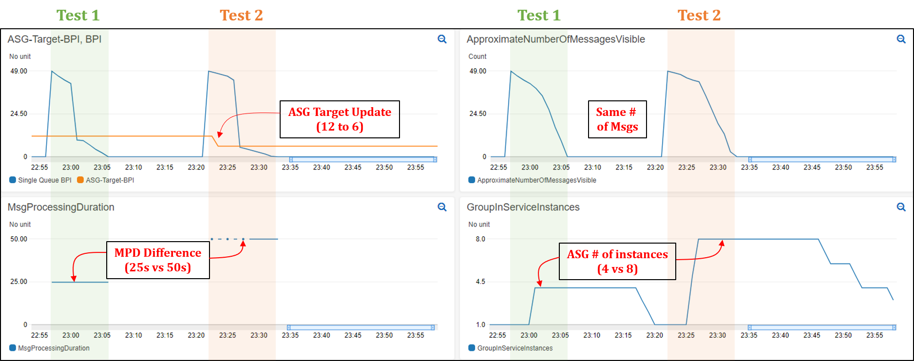
Figure 2: CloudWatch dashboard showing Auto Scaling group scaling test results (Test 1 and 2).
Recommended best practices for Auto Scaling groups
This section highlights a few key best practices that we recommend adopting when deploying and working with Auto Scaling groups.
Reducing cost using EC2 Spot instances
Amazon SQS helps build loosely coupled application architectures, while providing reliable asynchronous communication between the various layers/components of an application. If a worker node fails to process a message within the Amazon SQS message visibility time-out, then the message is returned to the queue and another worker node can pick up and process that message. This makes Amazon SQS-backed applications fault-tolerant by design and thus a great fit for EC2 Spot instances. EC2 spot instances are spare compute capacity in the AWS cloud that is available to you at steep discounts as compared to On-Demand prices.
Maximizing capacity using attribute-based instance selection
With the recently released attribute-based instance selection feature, you can define infrastructure requirements based on application needs such as vCPU, RAM, and processor family (e.g., x86, ARM). This removes the need to define specific instances in your Auto Scaling group configuration, and it eliminates the burden of identifying the correct instance families and sizes. In addition, newly released instance types will be automatically considered if they fit your requirements. Attribute-based instance selection lets you tap into hundreds of different EC2 instance pools, which increases the chance of getting EC2 (Spot/On-demand) instances. When using attribute-based instance selection with the capacity optimized allocation strategy, Amazon EC2 allocates instances from deeper Spot capacity pools, thereby further reducing the chance of Spot interruption.
The following sample configuration creates an Auto Scaling group with attribute-based instance selection:
AutoScalingGroupName: 'my-asg' # [REQUIRED]
MixedInstancesPolicy:
  LaunchTemplate:
    LaunchTemplateSpecification:
      LaunchTemplateId: 'lt-0537239d9aef10a77'
    Overrides:
    - InstanceRequirements:
        VCpuCount: # [REQUIRED]
          Min: 2
          Max: 4
        MemoryMiB: # [REQUIRED]
          Min: 2048
  InstancesDistribution:
    SpotAllocationStrategy: 'capacity-optimized'
MinSize: 0 # [REQUIRED]
MaxSize: 100 # [REQUIRED]
DesiredCapacity: 4
VPCZoneIdentifier: 'subnet-e76a128a,subnet-e66a128b,subnet-e16a128c'
Conclusion
As can be seen from the test results, this approach demonstrates how an Auto Scaling group can honor a user-provided acceptable latency constraint while accomodating variations in the MPD over time. This is possible because the average MPD is monitored and regularly updated as a CloudWatch metric. In turn, this is continously used to update the target value of the group’s target tracking policy. Moreover, we have covered additional Auto Scaling group best practices suitable for this use case, including the use of Spot instances to reduce costs and attribute-based instance selection to simplify the selection of relevant instance types.
For more information on scaling options for Auto Scaling groups, visit the Amazon EC2 Auto Scaling documentation page and the SQS-based scaling guide.