Tag Archives: Auto Scaling

Building diversified and cost-optimized EC2 server groups in Spinnaker

Post Syndicated from Sheila Busser original https://aws.amazon.com/blogs/compute/building-diversified-and-cost-optimized-ec2-server-groups-in-spinnaker/

This blog post is written by Sandeep Palavalasa, Sr. Specialist Containers SA, and Prathibha Datta-Kumar, Software Development Engineer

Spinnaker is an open source continuous delivery platform created by Netflix for releasing software changes rapidly and reliably. It enables teams to automate deployments into pipelines that are run whenever a new version is released with proven deployment strategies that are faster and more dependable with zero downtime. For many AWS customers, Spinnaker is a critical piece of technology that allows developers to deploy their applications safely and reliably across different AWS managed services.

Listening to customer requests on the Spinnaker open source project and in the Amazon EC2 Spot Instances integrations roadmap, we have further enhanced Spinnaker’s ability to deploy on Amazon Elastic Compute Cloud (Amazon EC2). The enhancements make it easier to combine Spot Instances with On-Demand, Reserved, and Savings Plans Instances to optimize workload costs with performance. You can improve workload availability when using Spot Instances with features such as allocation strategies and proactive Spot capacity rebalancing, when you are flexible about Instance types and Availability Zones. Combinations of these features offer the best possible experience when using Amazon EC2 with Spinnaker.

In this post, we detail the recent enhancements, along with a walkthrough of how you can use them following the best practices.

Amazon EC2 Spot Instances

EC2 Spot Instances are spare compute capacity in the AWS Cloud available at steep discounts of up to 90% when compared to On-Demand Instance prices. The primary difference between an On-Demand Instance and a Spot Instance is that a Spot Instance can be interrupted by Amazon EC2 with a two-minute notification when Amazon EC2 needs the capacity back. Amazon EC2 now sends rebalance recommendation notifications when Spot Instances are at an elevated risk of interruption. This signal can arrive sooner than the two-minute interruption notice. This lets you proactively replace your Spot Instances before it’s interrupted.

The best way to adhere to Spot best practices and instance fleet management is by using an Amazon EC2 Auto Scaling group When using Spot Instances in Auto Scaling group, enabling Capacity Rebalancing helps you maintain workload availability by proactively augmenting your fleet with a new Spot Instance before a running instance is interrupted by Amazon EC2.

Spinnaker concepts

Spinnaker uses three key concepts to describe your services, including applications, clusters, and server groups, and how your services are exposed to users is expressed as Load balancers and firewalls.

An application is a collection of clusters, a cluster is a collection of server groups, and a server group identifies the deployable artifact and basic configuration settings such as the number of instances, autoscaling policies, metadata, etc. This corresponds to an Auto Scaling group in AWS. We use Auto Scaling groups and server groups interchangeably in this post.

Spinnaker and Amazon EC2 Integration

In mid-2020, we started looking into customer requests and gaps in the Amazon EC2 feature set supported in Spinnaker. Around the same time, Spinnaker OSS added support for Amazon EC2 Launch Templates. Thanks to their effort, we could follow-up and expand the Amazon EC2 feature set supported in Spinnaker. Now that we understand the new features, let’s look at how to use some of them in the following tutorial spinnaker.io.

Here are some highlights of the features contributed recently:

Feature Why use it? (Example use cases)
  Multiple Instance Types   Tap into multiple capacity pools to achieve and maintain the desired scale using Spot Instances.
  Combining On-Demand and Spot Instances

  – Control the proportion of On-Demand and Spot Instances launched in your sever group.

– Combine Spot Instances with Amazon EC2 Reserved Instances or Savings Plans.

  Amazon EC2 Auto Scaling allocation strategies   Reduce overall Spot interruptions by launching from Spot pools that are optimally chosen based on the available Spot capacity, using capacity-optimized Spot allocation strategy.
  Capacity rebalancing   Improve your workload availability by proactively shifting your Spot capacity to optimal pools by enabling capacity rebalancing along with capacity-optimized allocation strategy.
  Improved support for burstable performance instance types with custom credit specification   Reduce costs by preventing wastage of CPU cycles.

We recommend using Spinnaker stable release 1.28.x for API users and 1.29.x for UI users. Here is the Git issue for related PRs and feature releases.

Now that we understand the new features, let’s look at how to use some of them in the following tutorial.

Example tutorial: Deploy a demo web application on an Auto Scaling group with On-Demand and Spot Instances

In this example tutorial, we setup Spinnaker to deploy to Amazon EC2, create an Application Load Balancer, and deploy a demo application on a server group diversified across multiple instance types and purchase options – this case On-Demand and Spot Instances.

We leverage Spinnaker’s API throughout the tutorial to create new resources, along with a quick guide on how to deploy the same using Spinnaker UI (Deck) and leverage UI to view them.

Prerequisites

As a prerequisite to complete this tutorial, you must have an AWS Account with an AWS Identity and Access Management (IAM) User that has the AdministratorAccess configured to use with AWS Command Line Interface (AWS CLI).

1. Spinnaker setup

We will use the AWS CloudFormation template setup-spinnaker-with-deployment-vpc.yml to setup Spinnaker and the required resources.

1.1 Create an Secure Shell(SSH) keypair used to connect to Spinnaker and EC2 instances launched by Spinnaker.

AWS_REGION=us-west-2 # Change the region where you want Spinnaker deployed
EC2_KEYPAIR_NAME=spinnaker-blog-${AWS_REGION}
aws ec2 create-key-pair --key-name ${EC2_KEYPAIR_NAME} --region ${AWS_REGION} --query KeyMaterial --output text > ~/${EC2_KEYPAIR_NAME}.pem
chmod 600 ~/${EC2_KEYPAIR_NAME}.pem

1.2 Deploy the Cloudformation stack.

STACK_NAME=spinnaker-blog
SPINNAKER_VERSION=1.29.1 # Change the version if newer versions are available
NUMBER_OF_AZS=3
AVAILABILITY_ZONES=${AWS_REGION}a,${AWS_REGION}b,${AWS_REGION}c
ACCOUNT_ID=$(aws sts get-caller-identity --query "Account" --output text)
S3_BUCKET_NAME=spin-persitent-store-${ACCOUNT_ID}

# Download template
curl -o setup-spinnaker-with-deployment-vpc.yml https://raw.githubusercontent.com/awslabs/ec2-spot-labs/master/ec2-spot-spinnaker/setup-spinnaker-with-deployment-vpc.yml

# deploy stack
aws cloudformation deploy --template-file setup-spinnaker-with-deployment-vpc.yml \
    --stack-name ${STACK_NAME} \
    --parameter-overrides NumberOfAZs=${NUMBER_OF_AZS} \
    AvailabilityZones=${AVAILABILITY_ZONES} \
    EC2KeyPairName=${EC2_KEYPAIR_NAME} \
    SpinnakerVersion=${SPINNAKER_VERSION} \
    SpinnakerS3BucketName=${S3_BUCKET_NAME} \
    --capabilities CAPABILITY_NAMED_IAM --region ${AWS_REGION}

1.3 Connecting to Spinnaker

1.3.1 Get the SSH command to port forwarding for Deck – the browser-based UI (9000) and Gate – the API Gateway (8084) to access the Spinnaker UI and API.

SPINNAKER_INSTANCE_DNS_NAME=$(aws cloudformation describe-stacks --stack-name ${STACK_NAME} --region ${AWS_REGION} --query "Stacks[].Outputs[?OutputKey=='SpinnakerInstance'].OutputValue" --output text)
echo 'ssh -A -L 9000:localhost:9000 -L 8084:localhost:8084 -L 8087:localhost:8087 -i ~/'${EC2_KEYPAIR_NAME}' [email protected]$'{SPINNAKER_INSTANCE_DNS_NAME}''

1.3.2 Open a new terminal and use the SSH command (output from the previous command) to connect to the Spinnaker instance. After you successfully connect to the Spinnaker instance via SSH, access the Spinnaker UI here and API here.

2. Deploy a demo web application

Let’s make sure that we have the environment variables required in the shell before proceeding. If you’re using the same terminal window as before, then you might already have these variables.

STACK_NAME=spinnaker-blog
AWS_REGION=us-west-2 # use the same region as before
EC2_KEYPAIR_NAME=spinnaker-blog-${AWS_REGION}
VPC_ID=$(aws cloudformation describe-stacks --stack-name ${STACK_NAME} --region ${AWS_REGION} --query "Stacks[].Outputs[?OutputKey=='VPCID'].OutputValue" --output text)

2.1 Create a Spinnaker Application

We start by creating an application in Spinnaker, a placeholder for the service that we deploy.

curl 'http://localhost:8084/tasks' \
-H 'Content-Type: application/json;charset=utf-8' \
--data-raw \
'{
   "job":[
      {
         "type":"createApplication",
         "application":{
            "cloudProviders":"aws",
            "instancePort":80,
            "name":"demoapp",
            "email":"[email protected]",
            "providerSettings":{
               "aws":{
                  "useAmiBlockDeviceMappings":true
               }
            }
         }
      }
   ],
   "application":"demoapp",
   "description":"Create Application: demoapp"
}'

Spin Create Server Group

2.2 Create an Application Load Balancer

Let’s create an Application Load Balanacer and a target group for port 80, spanning the three availability zones in our public subnet. We use the Demo-ALB-SecurityGroup for Firewalls to allow public access to the ALB on port 80.

As Spot Instances are interrupted with a two minute warning, you must adjust the Target Group’s deregistration delay to a slightly lower time. Recommended values are 90 seconds or less. This allows time for in-flight requests to complete and gracefully close existing connections before the instance is interrupted.

curl 'http://localhost:8084/tasks' \
-H 'Content-Type: application/json;charset=utf-8' \
--data-binary \
'{
   "application":"demoapp",
   "description":"Create Load Balancer: demoapp",
   "job":[
      {
         "type":"upsertLoadBalancer",
         "name":"demoapp-lb",
         "loadBalancerType":"application",
         "cloudProvider":"aws",
         "credentials":"my-aws-account",
         "region":"'"${AWS_REGION}"'",
         "vpcId":"'"${VPC_ID}"'",
         "subnetType":"public-subnet",
         "idleTimeout":60,
         "targetGroups":[
            {
               "name":"demoapp-targetgroup",
               "protocol":"HTTP",
               "port":80,
               "targetType":"instance",
               "healthCheckProtocol":"HTTP",
               "healthCheckPort":"traffic-port",
               "healthCheckPath":"/",
               "attributes":{
                  "deregistrationDelay":90
               }
            }
         ],
         "regionZones":[
            "'"${AWS_REGION}"'a",
            "'"${AWS_REGION}"'b",
            "'"${AWS_REGION}"'c"
         ],
         "securityGroups":[
            "Demo-ALB-SecurityGroup"
         ],
         "listeners":[
            {
               "protocol":"HTTP",
               "port":80,
               "defaultActions":[
                  {
                     "type":"forward",
                     "targetGroupName":"demoapp-targetgroup"
                 }
               ]
            }
         ]
      }
   ]
}'

Spin Create ALB

2.3 Create a server group

Before creating a server group (Auto Scaling group), here is a brief overview of the features used in the example:

      • onDemandBaseCapacity (default 0): The minimum amount of your ASG’s capacity that must be fulfilled by On-Demand instances (can also be applied toward Reserved Instances or Savings Plans). The example uses an onDemandBaseCapacity of three.
      • onDemandPercentageAboveBaseCapacity (default 100): The percentages of On-Demand and Spot Instances for additional capacity beyond OnDemandBaseCapacity. The example uses onDemandPercentageAboveBaseCapacity of 10% (i.e. 90% Spot).
      • spotAllocationStrategy: This indicates how you want to allocate instances across Spot Instance pools in each Availability Zone. The example uses the recommended Capacity Optimized strategy. Instances are launched from optimal Spot pools that are chosen based on the available Spot capacity for the number of instances that are launching.
      • launchTemplateOverridesForInstanceType: The list of instance types that are acceptable for your workload. Specifying multiple instance types enables tapping into multiple instance pools in multiple Availability Zones, designed to enhance your service’s availability. You can use the ec2-instance-selector, an open source AWS Command Line Interface(CLI) tool to narrow down the instance types based on resource criteria like vcpus and memory.
      • capacityRebalance: When enabled, this feature proactively manages the EC2 Spot Instance lifecycle leveraging the new EC2 Instance rebalance recommendation. This increases the emphasis on availability by automatically attempting to replace Spot Instances in an ASG before they are interrupted by Amazon EC2. We enable this feature in this example.

Learn more on spinnaker.io: feature descriptions and use cases and sample API requests.

Let’s create a server group with a desired capacity of 12 instances diversified across current and previous generation instance types, attach the previously created ALB, use Demo-EC2-SecurityGroup for the Firewalls which allows http traffic only from the ALB, use the following bash script for UserData to install httpd, and add instance metadata into the index.html.

2.3.1 Save the userdata bash script into a file user-date.sh.

Note that Spinnaker only support base64 encoded userdata. We use base64 bash command to encode the file contents in the next step.

cat << "EOF" > user-data.sh
#!/bin/bash
yum update -y
yum install httpd -y
echo "<html>
    <head>
        <title>Demo Application</title>
        <style>body {margin-top: 40px; background-color: #Gray;} </style>
    </head>
    <body>
        <h2>You have reached a Demo Application running on</h2>
        <ul>
            <li>instance-id: <b> `curl http://169.254.169.254/latest/meta-data/instance-id` </b></li>
            <li>instance-type: <b> `curl http://169.254.169.254/latest/meta-data/instance-type` </b></li>
            <li>instance-life-cycle: <b> `curl http://169.254.169.254/latest/meta-data/instance-life-cycle` </b></li>
            <li>availability-zone: <b> `curl http://169.254.169.254/latest/meta-data/placement/availability-zone` </b></li>
        </ul>
    </body>
</html>" > /var/www/html/index.html
systemctl start httpd
systemctl enable httpd
EOF

2.3.2 Create the server group by running the following command. Note we use the KeyPairName that we created as part of the prerequisites.

curl 'http://localhost:8084/tasks' \
-H 'Content-Type: application/json;charset=utf-8' \
-d \
'{
   "job":[
      {
         "type":"createServerGroup",
         "cloudProvider":"aws",
         "account":"my-aws-account",
         "application":"demoapp",
         "stack":"",
         "credentials":"my-aws-account",
	"healthCheckType": "ELB",
	"healthCheckGracePeriod":600,
	"capacityRebalance": true,
         "onDemandBaseCapacity":3, 
         "onDemandPercentageAboveBaseCapacity":10,
         "spotAllocationStrategy":"capacity-optimized",
         "setLaunchTemplate":true,
         "launchTemplateOverridesForInstanceType":[
            {
               "instanceType":"m4.large"
            },
            {
               "instanceType":"m5.large"
            },
            {
               "instanceType":"m5a.large"
            },
            {
               "instanceType":"m5ad.large"
            },
            {
               "instanceType":"m5d.large"
            },
            {
               "instanceType":"m5dn.large"
            },
            {
               "instanceType":"m5n.large"
            }

         ],
         "capacity":{
            "min":6,
            "max":21,
            "desired":12
         },
         "subnetType":"private-subnet",
         "availabilityZones":{
            "'"${AWS_REGION}"'":[
               "'"${AWS_REGION}"'a",
               "'"${AWS_REGION}"'b",
               "'"${AWS_REGION}"'c"
            ]
         },
         "keyPair":"'"${EC2_KEYPAIR_NAME}"'",
         "securityGroups":[
            "Demo-EC2-SecurityGroup"
         ],
         "instanceType":"m5.large",
         "virtualizationType":"hvm",
         "amiName":"'"$(aws ec2 describe-images --owners amazon --filters "Name=name,Values=amzn2-ami-hvm-2*x86_64-gp2" --query 'reverse(sort_by(Images, &CreationDate))[0].Name' --region ${AWS_REGION} --output text)"'",
         "targetGroups":[
            "demoapp-targetgroup"
         ],
         "base64UserData":"'"$(base64 user-data.sh)"'",,
        "associatePublicIpAddress":false,
         "instanceMonitoring":false
      }
   ],
   "application":"demoapp",
   "description":"Create New server group in cluster demoapp"
}'

Spin Create ServerGroup

Spinnaker creates an Amazon EC2 Launch Template and an ASG with specified parameters and waits until the ALB health check passes before sending traffic to the EC2 Instances.

The server group and launch template that we just created will look like this in Spinnaker UI:

Spin View ServerGroup

The UI also displays capacity type, such as the purchase option for each instance type in the Instance Information section:

Spin View ServerGroup Purchase Options 1Spin View ServerGroup Purchase Options 2

3. Access the application

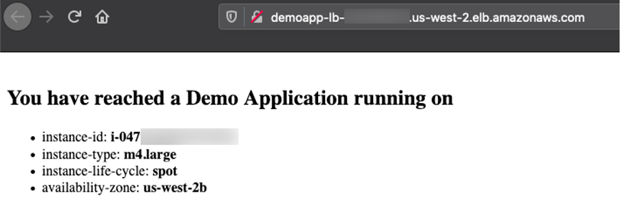
Copy the Application Load Balancer URL by selecting the tree icon in the right top corner of the server group, and access it in a browser. You can refresh multiple times to see that the requests are going to different instances every time.

Spin Access App

Congratulations! You successfully deployed the demo application on an Amazon EC2 server group diversified across multiple instance types and purchase options.

Moreover, you can clone, modify, disable, and destroy these server groups, as well as use them with Spinnaker pipelines to effectively release new versions of your application.
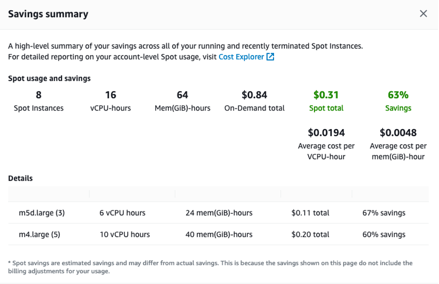
Cost savings

Check the savings you realized by deploying your demo application on EC2 Spot Instances by going to EC2 console > Spot Requests > Saving Summary.

Spin Spot Savings

Cleanup

To avoid incurring any additional charges, clean up the resources created in the tutorial.

Frist, delete the server group, application load balancer and application in Spinnaker.

curl 'http://localhost:8084/tasks' \
-H 'Content-Type: application/json;charset=utf-8' \
--data-raw \
'{
   "job":[
      {
         "reason":"Cleanup",
         "asgName":"demoapp-v000",
         "moniker":{
            "app":"demoapp",
            "cluster":"demoapp",
            "sequence":0
         },
         "serverGroupName":"demoapp-v000",
         "type":"destroyServerGroup",
         "region":"'"${AWS_REGION}"'",
         "credentials":"my-aws-account",
         "cloudProvider":"aws"
      },
      {
         "cloudProvider":"aws",
         "loadBalancerName":"demoapp-lb",
         "loadBalancerType":"application",
         "regions":[
            "'"${AWS_REGION}"'"
         ],
         "credentials":"my-aws-account",
         "vpcId":"'"${VPC_ID}"'",
         "type":"deleteLoadBalancer"
      },
      {
         "type":"deleteApplication",
         "application":{
            "name":"demoapp",
            "cloudProviders":"aws"
         }
      }
   ],
   "application":"demoapp",
   "description":"Deleting ServerGroup, ALB and Application: demoapp"
}'

Wait for Spinnaker to delete all of the resources before proceeding further. You can confirm this either on the Spinnaker UI or AWS Management Console.

Then delete the Spinnaker infrastructure by running the following command:

aws ec2 delete-key-pair --key-name ${EC2_KEYPAIR_NAME} --region ${AWS_REGION}
rm ~/${EC2_KEYPAIR_NAME}.pem
aws s3api delete-objects \
--bucket ${S3_BUCKET_NAME} \
--delete "$(aws s3api list-object-versions \
--bucket ${S3_BUCKET_NAME} \
--query='{Objects: Versions[].{Key:Key,VersionId:VersionId}}')" #If error occurs, there are no Versions and is OK
aws s3api delete-objects \
--bucket ${S3_BUCKET_NAME} \
--delete "$(aws s3api list-object-versions \
--bucket ${S3_BUCKET_NAME} \
--query='{Objects: DeleteMarkers[].{Key:Key,VersionId:VersionId}}')" #If error occurs, there are no DeleteMarkers and is OK
aws s3 rb s3://${S3_BUCKET_NAME} --force #Delete Bucket
aws cloudformation delete-stack --region ${AWS_REGION} --stack-name ${STACK_NAME}

Conclusion

In this post, we learned about the new Amazon EC2 features recently added to Spinnaker, and how to use them to build diversified and optimized Auto Scaling Groups. We also discussed recommended best practices for EC2 Spot and how they can improve your experience with it.

We would love to hear from you! Tell us about other Continuous Integration/Continuous Delivery (CI/CD) platforms that you want to use with EC2 Spot and/or Auto Scaling Groups by adding an issue on the Spot integrations roadmap.

AWS Week in Review – March 20, 2023

Post Syndicated from Danilo Poccia original https://aws.amazon.com/blogs/aws/aws-week-in-review-march-20-2023/

This post is part of our Week in Review series. Check back each week for a quick roundup of interesting news and announcements from AWS!

A new week starts, and Spring is almost here! If you’re curious about AWS news from the previous seven days, I got you covered.

Last Week’s Launches
Here are the launches that got my attention last week:

Picture of an S3 bucket and AWS CEO Adam Selipsky.Amazon S3 – Last week there was AWS Pi Day 2023 celebrating 17 years of innovation since Amazon S3 was introduced on March 14, 2006. For the occasion, the team released many new capabilities:

Amazon Linux 2023 – Our new Linux-based operating system is now generally available. Sébastien’s post is full of tips and info.

Application Auto Scaling – Now can use arithmetic operations and mathematical functions to customize the metrics used with Target Tracking policies. You can use it to scale based on your own application-specific metrics. Read how it works with Amazon ECS services.

AWS Data Exchange for Amazon S3 is now generally available – You can now share and find data files directly from S3 buckets, without the need to create or manage copies of the data.

Amazon Neptune – Now offers a graph summary API to help understand important metadata about property graphs (PG) and resource description framework (RDF) graphs. Neptune added support for Slow Query Logs to help identify queries that need performance tuning.

Amazon OpenSearch Service – The team introduced security analytics that provides new threat monitoring, detection, and alerting features. The service now supports OpenSearch version 2.5 that adds several new features such as support for Point in Time Search and improvements to observability and geospatial functionality.

AWS Lake Formation and Apache Hive on Amazon EMR – Introduced fine-grained access controls that allow data administrators to define and enforce fine-grained table and column level security for customers accessing data via Apache Hive running on Amazon EMR.

Amazon EC2 M1 Mac Instances – You can now update guest environments to a specific or the latest macOS version without having to tear down and recreate the existing macOS environments.

AWS Chatbot – Now Integrates With Microsoft Teams to simplify the way you troubleshoot and operate your AWS resources.

Amazon GuardDuty RDS Protection for Amazon Aurora – Now generally available to help profile and monitor access activity to Aurora databases in your AWS account without impacting database performance

AWS Database Migration Service – Now supports validation to ensure that data is migrated accurately to S3 and can now generate an AWS Glue Data Catalog when migrating to S3.

AWS Backup – You can now back up and restore virtual machines running on VMware vSphere 8 and with multiple vNICs.

Amazon Kendra – There are new connectors to index documents and search for information across these new content: Confluence Server, Confluence Cloud, Microsoft SharePoint OnPrem, Microsoft SharePoint Cloud. This post shows how to use the Amazon Kendra connector for Microsoft Teams.

For a full list of AWS announcements, be sure to keep an eye on the What’s New at AWS page.

Other AWS News
A few more blog posts you might have missed:

Example of a geospatial query.Women founders Q&A – We’re talking to six women founders and leaders about how they’re making impacts in their communities, industries, and beyond.

What you missed at that 2023 IMAGINE: Nonprofit conference – Where hundreds of nonprofit leaders, technologists, and innovators gathered to learn and share how AWS can drive a positive impact for people and the planet.

Monitoring load balancers using Amazon CloudWatch anomaly detection alarms – The metrics emitted by load balancers provide crucial and unique insight into service health, service performance, and end-to-end network performance.

Extend geospatial queries in Amazon Athena with user-defined functions (UDFs) and AWS Lambda – Using a solution based on Uber’s Hexagonal Hierarchical Spatial Index (H3) to divide the globe into equally-sized hexagons.

How cities can use transport data to reduce pollution and increase safety – A guest post by Rikesh Shah, outgoing head of open innovation at Transport for London.

For AWS open-source news and updates, here’s the latest newsletter curated by Ricardo to bring you the most recent updates on open-source projects, posts, events, and more.

Upcoming AWS Events
Here are some opportunities to meet:

AWS Public Sector Day 2023 (March 21, London, UK) – An event dedicated to helping public sector organizations use technology to achieve more with less through the current challenging conditions.

Women in Tech at Skills Center Arlington (March 23, VA, USA) – Let’s celebrate the history and legacy of women in tech.

The AWS Summits season is warming up! You can sign up here to know when registration opens in your area.

That’s all from me for this week. Come back next Monday for another Week in Review!

Danilo

How to create custom health checks for your Amazon EC2 Auto Scaling Fleet

Post Syndicated from Sheila Busser original https://aws.amazon.com/blogs/compute/how-to-create-custom-health-checks-for-your-amazon-ec2-auto-scaling-fleet/

This blog post is written by Gaurav Verma, Cloud Infrastructure Architect, Professional Services AWS.

Amazon EC2 Auto Scaling helps you maintain application availability and lets you automatically add or remove Amazon Elastic Compute Cloud (Amazon EC2) instances according to the conditions that you define. You can use dynamic and predictive scaling to scale-out and scale-in EC2 instances. Auto Scaling helps to maintain the self-healing Amazon EC2 environment for an application where Auto Scaling can use the status of Amazon EC2 health checks to determine if an instance is faulty and needs replacement. Amazon EC2 Auto Scaling provides three types of health checks, which are discussed below.

EC2 Status check: AWS provides two types of health checks for EC2 instances: System status check and instance status check. System status checks monitor the AWS system on which an instance is running. If the problem is with underlying system, AWS will fix the problem. Instance status check monitors the software and network configuration of an instance. If the instance status check fails, then you can fix the problem by following the steps in the troubleshoot instances with failed status checks documentation.

Elastic Load Balancer Health Check: Auto Scaling groups are generally connected to Elastic Load Balancers (ELB). ELB provides the application-level health check by monitoring the endpoint (a webpage, or a health page in a web application) of an application. ELB health check monitors the application and marks the instance unhealthy if there is no response from an instance in the configured time.

Custom Health Check: You can use custom health checks to mark any instance as unhealthy if the instance fails for the check you define. Custom health checks can be used to implement various user requirements, such as the presence of instance tags added upon completion of a required workflow. The user data script is executed at instance boot time, and it can perform additional investigation into whether or not the user requirements are met before confirming that the instance is ready to accept load. For example, this approach could be used to confirm that the instance was successfully integrated with other parts of a complex application stack.

In some cases, a customer may add multiple checks either in the Amazon EC2 AMI or in the boot sequence to keep the instance secure and compliant. These checks can increase the boot time for the EC2 instance, and they can reboot the EC2 instance multiple times before an instance can be marked as compliant. Therefore, in some cases, an EC2 instance boot period can take forty to fifty minutes or longer.

If an EC2 instance isn’t marked as healthy within a defined time, Auto Scaling will mark an instance unhealthy, even though the instance wasn’t yet ready for evaluation. Custom health checks can help manage these situations. You can write the Amazon EC2 user data script to perform the custom health check and force Auto Scaling to wait until the instance is truly healthy (i.e., functional, secure, and compliant).

This blog describes a method to write a custom health check. We write an Amazon EC2 user data script to perform the custom health check and automate it for future EC2 instances in the Auto Scaling group. This script can wait for an instance to successfully complete the boot process and then mark the instance as healthy.

Prerequisites

You must have an AWS Identity and Access Management (IAM) role for Amazon EC2 with an Auto Scaling policy, which has these two actions allowed for the Auto Scaling group:

autoscaling:CompleteLifecycleAction

autoscaling:RecordLifecycleActionHeartbeat

Furthermore, we use the Amazon EC2 Auto Scaling lifecycle hooks. Lifecycle hooks let you create a solutions that are aware of events in Auto Scaling instance lifecycle, and then perform a custom action on instances when the lifecycle event occurs. As mentioned previously, typically a custom health check is needed when determining the workload readiness of an instance would be longer than the usual boot time for an EC2 instance that Auto Scaling assumes. Therefore, we utilize lifecycle hooks to keep the checks running until the instance is marked healthy.

Create custom health check

Let’s look at an example where an instance can only be marked as healthy if the instance has a tag with the key “Compliance-Check” and value “Successful”. Until this tag is both (a) present and (b) carries the value “Successful”, the instance shouldn’t be marked as “InService”.

  1. Create the Auto Scaling launch template for Amazon EC2 Auto Scaling. Name your Launch template “test”. In the additional configuration for user data, use this shell script as text.

The Following script will install the AWS Command Line Interface (AWS CLI) to interact with the AWS tagging and Auto Scaling APIs. Then, the script will run the while loop until the instance has a tag with the key “Compliance-Check” and value “Successful”. Once the instance has a tag, it will mark the instance as healthy and the instance will move into the “InService” state.

#!/bin/bash
curl "https://awscli.amazonaws.com/awscli-exe-linux-x86_64.zip" -o "awscliv2.zip"
unzip awscliv2.zip
sudo ./aws/install
#get instance id
instance=$(curl http://169.254.169.254/latest/meta-data/instance-id)

#Checking instance status
while true
do
readystatus=$(aws ec2 describe-instances --instance-ids $instance --filters "Name=tag: Compliance-Check,Values= Successful" |grep -i $instance)
if [[ $readystatus = *"InstanceId"* ]]; then
        echo $readystatus >> /home/ec2-user/user-script-output.txt
        aws autoscaling set-instance-health --instance-id $instance --health-status Healthy
        aws autoscaling complete-lifecycle-action --lifecycle-action-result CONTINUE --instance-id $instance --lifecycle-hook-name test --auto-scaling-group-name my-asg
        break 
else
	aws autoscaling set-instance-health --instance-id $instance --health-status Unhealthy
	sleep 5  
fi

done
  1. Create an Amazon EC2 Auto Scaling group using the AWS CLI with the “test” launch template that you just created and a predefined lifecycle hook. First, create a JSON file “config.json” in a system where you will run the AWS command to create the Auto Scaling group.
{
    "AutoScalingGroupName": "my-asg",
    "LaunchTemplate": {"LaunchTemplateId": "lt-1234567890abcde12"} ,
    "MinSize": 2,
    "MaxSize": 4,
    "DesiredCapacity": 2,
    "VPCZoneIdentifier": "subnet-12345678, subnet-90123456",
    "NewInstancesProtectedFromScaleIn": true,
    "LifecycleHookSpecificationList": [
        {
            "LifecycleHookName": "test",
            "LifecycleTransition": "autoscaling:EC2_INSTANCE_LAUNCHING",
            "HeartbeatTimeout": 300,
            "DefaultResult": "ABANDON"
        }
    ],
    "Tags": [
        {
            "ResourceId": "my-asg",
            "ResourceType": "auto-scaling-group",
            "Key": "Compliance-Check",
            "Value": "UnSuccessful",
            "PropagateAtLaunch": true
        }
    ]
}

To create the Auto Scaling group with the AWS CLI, you must run the following command at the same location where you saved the preceding JSON file. Make sure to replace the relevant subnets that you intend to use in the VPCZoneIdentifier.

>> aws autoscaling create-auto-scaling-group –cli-input-json file://config.json

This command will create the Auto Scaling group with a configuration defined in the JSON file. This Auto Scaling group should have two instances and a lifecycle hook called “test” with a 300 second wait period at the time of launch of an instance.

Tests

Now is the time to test the newly-created instances with a custom health check. Instances in Auto Scaling should be in the “Pending:Wait” stage, not the “InService” stage. Instances will be in this stage for approximately five minutes because we have a lifecycle hook time of 300 seconds in the config.json file.

If the workload readiness evaluation takes more than 300 seconds in your environment, then you can increase the lifecycle hook period to as long as 7200 seconds.

Change the tag value for one instance from “UnSuccessful” to “Successful”. If you’ve changed the tag within the five minutes of instances creation, then the instance should be in the “InService” state and marked as healthy.

Change Compliance-Check value from "UnSuccessful" to "Successful".

This test is a simulation of the situation where the health check of an instance depends on the tag values, and the tag values are only updated if the instance passes all of the checks as per the organization standards. Here we change the tag value manually, but in a real use case scenario, this value would be changed by the booting process when instances are marked as compliant.

Another test case could be that an instance should be marked as healthy if it’s added to the configuration management database, but not before that. For these checks, you can use the API with the curl command and look for the desired result. An example to call an API is in the above script, where it calls the AWS API to get the instance ID.

In case your custom health check script needs more than 7200 seconds, you can use this command to increase the lifecycle hook time:

>> aws autoscaling record-lifecycle-action-heartbeat –lifecycle-hook-name <lh_
name> –auto-scaling-group-name <asg_name> –instance-id <instance_id>

This command will give you the extra time equal to the time that you have configured in the life cycle hook.

Cleanup

Once you successfully test the solution, to avoid ongoing charges for resources you created, you should delete the resources.

To delete the Amazon EC2 Auto Scaling group, run the following command:

aws autoscaling delete-auto-scaling-group --auto-scaling-group-name my-asg

To delete the launch template, run the following command:

aws ec2 delete-launch-template --launch-template-id lt-1234567890abcde12

Delete the role and policy as well if you no longer need it.

Conclusion

EC2 Auto Scaling custom health checks are useful when system or instance health is insufficient, and you want instances to be marked as healthy only after additional checks. Typically, because of these different checks, the Amazon EC2 boot period can be longer than usual, and this may impact the scale-out process when an application needs more resources.

You can start by exploring EC2 Auto Scaling warm pools for these environments. You can keep the healthy marked instances in the warm pool in the Stopped stage. Then, these instances can be brought into the main pool at the time of scale-out without spending time on the boot process and lengthy health check. If you enable scale-in protection, then these healthy instances can move back to the warm pool at the time of scale-in rather than being terminated altogether.

Scaling an ASG using target tracking with a dynamic SQS target

Post Syndicated from Sheila Busser original https://aws.amazon.com/blogs/compute/scaling-an-asg-using-target-tracking-with-a-dynamic-sqs-target/

This blog post is written by Wassim Benhallam, Sr Cloud Application Architect AWS WWCO ProServe, and Rajesh Kesaraju, Sr. Specialist Solution Architect, EC2 Flexible Compute.

Scaling an Amazon EC2 Auto Scaling group based on Amazon Simple Queue Service (Amazon SQS) is a commonly used design pattern in decoupled applications. For example, an EC2 Auto Scaling Group can be used as a worker tier to offload the processing of audio files, images, or other files sent to the queue from an upstream tier (e.g., web tier). For latency-sensitive applications, AWS guidance describes a common pattern that allows an Auto Scaling group to scale in response to the backlog of an Amazon SQS queue while accounting for the average message processing duration (MPD) and the application’s desired latency.

This post builds on that guidance to focus on latency-sensitive applications where the MPD varies over time. Specifically, we demonstrate how to dynamically update the target value of the Auto Scaling group’s target tracking policy based on observed changes in the MPD. We also cover the utilization of Amazon EC2 Spot instances, mixed instance policies, and attribute-based instance selection in the Auto Scaling Groups as well as best practice implementation to achieve greater cost savings.

The challenge

The key challenge that this post addresses is applications that fail to honor their acceptable/target latency in situations where the MPD varies over time. Latency refers here to the time required for any queue message to be consumed and fully processed.

Consider the example of a customer using a worker tier to process image files (e.g., resizing, rescaling, or transformation) uploaded by users within a target latency of 100 seconds. The worker tier consists of an Auto Scaling group configured with a target tracking policy. To achieve the target latency mentioned previously, the customer assumes that each image can be processed in one second, and configures the target value of the scaling policy so that the average image backlog per instance is maintained at approximately 100 images.

In the first week, the customer submits 1000 images to the Amazon SQS queue for processing, each of which takes one second of processing time. Therefore, the Auto Scaling group scales to 10 instances, each of which processes 100 images in 100s, thereby honoring the target latency of 100s.

In the second week, the customer submits 1000 slightly larger images for processing. Since an image’s processing duration scales with its size, each image takes two seconds to process. As in the first week, the Auto Scaling group scales to 10 instances, but this time each instance processes 100 images in 200s, which is twice as long as was needed in the first round. As a result, the application fails to process the latter images within its acceptable latency.

Therefore, the challenge is common to any latency-sensitive application where the MPD is subject to change. Applications where the processing duration scales with input data size are particularly vulnerable to this problem. This includes image processing, document processing, computational jobs, and others.

Solution overview

Before we dive into the solution, let’s briefly review the target tracking policy’s scaling metric and its corresponding target value. A target tracking scaling policy works by adjusting the capacity to keep a scaling metric at, or close to, the specified target value. When scaling in response to an Amazon SQS backlog, it’s good practice to use a scaling metric known as the Backlog Per Instance (BPI) and a target value based on the acceptable BPI. These are computed as follows:

BPI equation, Saling metric and target value.

Given the acceptable BPI equation, a longer MPD requires us to use a smaller target value if we are to process these messages in the same acceptable latency, and vice versa. Therefore, the solution we propose here works by monitoring the average MPD over time and dynamically adjusting the target value of the Auto Scaling group’s target tracking policy (acceptable BPI) based on the observed changes in the MPD. This allows the scaling policy to adapt to variations in the average MPD over time, and thus enables the application to honor its acceptable latency.

Solution architecture

To demonstrate how the approach above can be implemented in practice, we put together an example architecture highlighting the services involved (see the following figure). We also provide an automated deployment solution for this architecture using an AWS Serverless Application Model (AWS SAM) template and some Python code (repository link). The repository also includes a README file with detailed instructions that you can follow to deploy the solution. The AWS SAM template deploys several resources, including an autoscaling group, launch template, target tracking scaling policy, an Amazon SQS queue, and a few AWS Lambda functions that serve various functions described as follows.

The Amazon SQS queue is used to accumulate messages intended for processing, while the Auto Scaling group instances are responsible for polling the queue and processing any messages received. To do this, a launch template defines a bootstrap script that allows the group’s instances to download and execute a Python code when first launched. The Python code consumes messages from the Amazon SQS queue and simulates their processing by sleeping for the MPD duration specified in the message body. After processing each message, the instance publishes the MPD as an Amazon CloudWatch metric (see the following figure).

Figure 1: Architecture diagram showing the components deployed by the AWS SAM template. These include an SQS queue, an Auto Scaling group responsible for polling and processing queue messages, a Lambda function that regularly updates the BPI CloudWatch metric, and a “Target Setter” Lambda function that regularly updates the Auto Scaling group’s target tracking scaling policy.

Figure 1: Architecture diagram showing the components deployed by the AWS SAM template.

To enable scaling, the Auto Scaling group is configured with a target tracking scaling policy that specifies BPI as the scaling metric and with an initial target value provided by the user.

The BPI CloudWatch metric is calculated and published by the “Metric-Publisher” Lambda function which is invoked every one minute using an Amazon EventBridge rate expression. To calculate BPI, the Lambda function simply takes the ratio of the number of messages visible in the Amazon SQS queue by the total number of in-service instances in the Auto Scaling group, as shown in equation (2) above.

On the other hand, the scaling policy’s target value is updated by the “Target-Setter” Lambda function, which is invoked every 30 minutes using another EventBridge rate expression. To calculate the new target value, the Lambda function simply takes the ratio of the user-defined acceptable latency value by the current average MPD queried from the corresponding CloudWatch metric, as shown in the previous equation (1).

Finally, to help you quickly test this solution, a Lambda function “Testing Lambda” is also provided and can be used to send messages to the Amazon SQS queue with a processing duration of your choice. This is specified within each message’s body. You can invoke this Lambda function with different MPDs (by modifying the corresponding environment variable) to verify how the Auto Scaling group scales in response. A CloudWatch dashboard is also deployed to enable you to track key scaling metrics through time. These include the number of messages visible in the queue, the number of in-service instances in the Auto Scaling group, the MPD, and BPI vs acceptable BPI.

Solution testing

To demonstrate the solution in action and its impact on application latency, we conducted two tests that you can reproduce by following the instructions described in the “Testing” section of the repository’s README file (repository link). In both tests, we assume a hypothetical application with a target latency of 300s. We also modified the invocation frequency of the “Target Setter” Lambda function to one minute to quickly assess the impact of target value changes. In both tests, we submit 50 messages to the Amazon SQS queue through the provided helper lambda. An MPD of 25s and 50s was used for the first and second test, respectively. The provided CloudWatch dashboard shows that the ASG scales to a total of four instances in the first test, and eight instances in the second (see the following figure). See README file for a detailed description of how various metrics evolve over time.

Comparison of Tests 1 and 2

Since Test 2 messages take twice as long to process, the Auto Scaling group launched twice as many instances to attempt to process all of the messages in the same amount of time as Test 1 (latency). The following figure shows that the total time to process all 50 messages in Test 1 was 9 mins vs 10 mins in Test 2. In contrast, if we were to use a static/fixed acceptable BPI of 12, then a total of four instances would have been operational in Test 2, thereby requiring double the time of Test 1 (~20 minutes) to process all of the messages. This demonstrates the value of using a dynamic scaling target when processing messages from Amazon SQS queues, especially in circumstances where the MPD is prone to vary with time.

Figure 2: CloudWatch dashboard showing Auto Scaling group scaling test results (Test 1 and 2). Although Test 2 messages require double the MPD of Test 1 messages, the Auto Scaling group processed Test 2 messages in the same amount of time as Test 1 by launching twice as many instances.

Figure 2: CloudWatch dashboard showing Auto Scaling group scaling test results (Test 1 and 2).

Recommended best practices for Auto Scaling groups

This section highlights a few key best practices that we recommend adopting when deploying and working with Auto Scaling groups.

Reducing cost using EC2 Spot instances

Amazon SQS helps build loosely coupled application architectures, while providing reliable asynchronous communication between the various layers/components of an application. If a worker node fails to process a message within the Amazon SQS message visibility time-out, then the message is returned to the queue and another worker node can pick up and process that message. This makes Amazon SQS-backed applications fault-tolerant by design and thus a great fit for EC2 Spot instances. EC2 spot instances are spare compute capacity in the AWS cloud that is available to you at steep discounts as compared to On-Demand prices.

Maximizing capacity using attribute-based instance selection

With the recently released attribute-based instance selection feature, you can define infrastructure requirements based on application needs such as vCPU, RAM, and processor family (e.g., x86, ARM). This removes the need to define specific instances in your Auto Scaling group configuration, and it eliminates the burden of identifying the correct instance families and sizes. In addition, newly released instance types will be automatically considered if they fit your requirements. Attribute-based instance selection lets you tap into hundreds of different EC2 instance pools, which increases the chance of getting EC2 (Spot/On-demand) instances. When using attribute-based instance selection with the capacity optimized allocation strategy, Amazon EC2 allocates instances from deeper Spot capacity pools, thereby further reducing the chance of Spot interruption.

The following sample configuration creates an Auto Scaling group with attribute-based instance selection:

AutoScalingGroupName: 'my-asg' # [REQUIRED] 
MixedInstancesPolicy:
  LaunchTemplate:
    LaunchTemplateSpecification:
      LaunchTemplateId: 'lt-0537239d9aef10a77'
    Overrides:
    - InstanceRequirements:
        VCpuCount: # [REQUIRED] 
          Min: 2
          Max: 4
        MemoryMiB: # [REQUIRED] 
          Min: 2048
  InstancesDistribution:
    SpotAllocationStrategy: 'capacity-optimized'
MinSize: 0 # [REQUIRED] 
MaxSize: 100 # [REQUIRED] 
DesiredCapacity: 4
VPCZoneIdentifier: 'subnet-e76a128a,subnet-e66a128b,subnet-e16a128c'

Conclusion

As can be seen from the test results, this approach demonstrates how an Auto Scaling group can honor a user-provided acceptable latency constraint while accomodating variations in the MPD over time. This is possible because the average MPD is monitored and regularly updated as a CloudWatch metric. In turn, this is continously used to update the target value of the group’s target tracking policy. Moreover, we have covered additional Auto Scaling group best practices suitable for this use case, including the use of Spot instances to reduce costs and attribute-based instance selection to simplify the selection of relevant instance types.

For more information on scaling options for Auto Scaling groups, visit the Amazon EC2 Auto Scaling documentation page and the SQS-based scaling guide.

Adopt Recommendations and Monitor Predictive Scaling for Optimal Compute Capacity

Post Syndicated from Sheila Busser original https://aws.amazon.com/blogs/compute/evaluating-predictive-scaling-for-amazon-ec2-capacity-optimization/

This post is written by Ankur Sethi, Sr. Product Manager, EC2, and Kinnar Sen, Sr. Specialist Solution Architect, AWS Compute.

Amazon EC2 Auto Scaling helps customers optimize their Amazon EC2 capacity by dynamically responding to varying demand. Based on customer feedback, we enhanced the scaling experience with the launch of predictive scaling policies. Predictive scaling proactively adds EC2 instances to your Auto Scaling group in anticipation of demand spikes. This results in better availability and performance for your applications that have predictable demand patterns and long initialization times. We recently launched a couple of features designed to help you assess the value of predictive scaling – prescriptive recommendations on whether to use predictive scaling based on its potential availability and cost impact, and integration with Amazon CloudWatch to continuously monitor the accuracy of predictions. In this post, we discuss the features in detail and the steps that you can easily adopt to enjoy the benefits of predictive scaling.

Recap: Predictive Scaling

EC2 Auto Scaling helps customers maintain application availability by managing the capacity and health of the underlying cluster. Prior to predictive scaling, EC2 Auto Scaling offered dynamic scaling policies such as target tracking and step scaling. These dynamic scaling policies are configured with an Amazon CloudWatch metric that represents an application’s load. EC2 Auto Scaling constantly monitors this metric and responds according to your policies, thereby triggering the launch or termination of instances. Although it’s extremely effective and widely used, this model is reactive in nature, and for larger spikes, may lead to unfulfilled capacity momentarily as the cluster is scaling out. Customers mitigate this by adopting aggressive scale out and conservative scale in to manage the additional buffer of instances. However, sometimes applications take a long time to initialize or have a recurring pattern with a sudden spike of high demand. These can have an impact on the initial response of the system when it is scaling out. Customers asked for a proactive scaling mechanism that can scale capacity ahead of predictable spikes, and so we delivered predictive scaling.

Predictive scaling was launched to make the scaling action proactive as it anticipates the changes required in the compute demand and scales accordingly. The scaling action is determined by ensemble machine learning (ML) built with data from your Auto Scaling group’s scaling patterns, as well as billions of data points from our observations. Predictive scaling should be used for applications where demand changes rapidly but with a recurring pattern, instances require a long time to initialize, or where you’re manually invoking scheduled scaling for routine demand patterns. Predictive scaling not only forecasts capacity requirements based on historical usage, but also learns continuously, thereby making forecasts more accurate with time. Furthermore, predictive scaling policy is designed to only scale out and not scale in your Auto Scaling groups, eliminating the risk of ending with lesser capacity because of inexact predictions. You must use dynamic scaling policy, scheduled scaling, or your own custom mechanism for scale-ins. In case of exceptional demand spikes, this addition of dynamic scaling policy can also improve your application performance by bridging the gap between demand and predicted capacity.

What’s new with predictive scaling

Predictive scaling policies can be configured in a non-mutative ‘Forecast Only’ mode to evaluate the accuracy of forecasts. When you’re ready to start scaling, you can switch to the ‘Forecast and Scale’ mode. Now we prescriptively recommend whether your policy should be switched to ‘Forecast and Scale’ mode if it can potentially lead to better availability and lower costs, saving you the time and effort of doing such an evaluation manually. You can test different configurations by creating multiple predictive scaling policies in ‘Forecast Only’ mode, and choose the one that performs best in terms of availability and cost improvements.

Monitoring and observability are key elements of AWS Well Architected Framework. Now we also offer CloudWatch metrics for your predictive scaling policies so that that you can programmatically monitor your predictive scaling policy for demand pattern changes or prolonged periods of inaccurate predictions. This will enable you to monitor the key performance metrics and make it easier to adopt AWS Well-Architected best practices.

In the following sections, we deep dive into the details of these two features.

Recommendations for predictive scaling

Once you set up an Auto Scaling group with predictive scaling policy in Forecast Only mode as explained in this introduction to predictive scaling blog post , you can review the results of the forecast visually and adjust any parameters to more accurately reflect the behavior that you desire. Evaluating simply on the basis of visualization may not be very intuitive if the scaling patterns are erratic. Moreover, if you keep higher minimum capacities, then the graph may show a flat line for the actual capacity as your Auto Scaling group capacity is an outcome of existing scaling policy configurations and the minimum capacity that you configured. This makes it difficult to contemplate whether the lower capacity predicted by predictive scaling wouldn’t leave your Auto Scaling group under-scaled.

This new feature provides a prescriptive guidance to switch on predictive scaling in Forecast and Scale mode based on the factors of availability and cost savings. To determine the availability and cost savings, we compare the predictions against the actual capacity and the optimal, required capacity. This required capacity is inferred based on whether your instances were running at a higher or lower value than the target value for scaling metric that you defined as part of the predictive scaling policy configuration. For example, if an Auto Scaling group is running 10 instances at 20% CPU Utilization while the target defined in predictive scaling policy is 40%, then the instances are running under-utilized by 50% and the required capacity is assumed to be 5 instances (half of your current capacity). For an Auto Scaling group, based on the time range in which you’re interested (two weeks as default), we aggregate the cost saving and availability impact of predictive scaling. The availability impact measures for the amount of time that the actual metric value was higher than the target value that you defined to be optimal for each policy. Similarly, cost savings measures the aggregated savings based on the capacity utilization of the underlying Auto Scaling group for each defined policy. The final cost and availability will lead us to a recommendation based on:

  • If availability increases (or remains same) and cost reduces (or remains same), then switch on Forecast and Scale
  • If availability reduces, then disable predictive scaling
  • If availability increase comes at an increased cost, then the customer should take the call based on their cost-availability tradeoff threshold

This figure shows the console view of how the recommendations look like on the Auto Scaling console. For each policy we make prescriptive recommendation of whether to switch to Forecast And Scale mode along with whether doing so can lead to better availability and lower costFigure 1: Predictive Scaling Recommendations on EC2 Auto Scaling console

The preceding figure shows how the console reflects the recommendation for a predictive scaling policy. You get information on whether the policy can lead to higher availability and lower cost, which leads to a recommendation to switch to Forecast and Scale. To achieve this cost saving, you might have to lower your minimum capacity and aim for higher utilization in dynamic scaling policies.

To get the most value from this feature, we recommend that you create multiple predictive scaling policies in Forecast Only mode with different configurations, choosing different metrics and/or different target values. Target value is an important lever that changes how aggressive the capacity forecasts must be. A lower target value increases your capacity forecast resulting in better availability for your application. However, this also means more dollars to be spent on the Amazon EC2 cost. Similarly, a higher target value can leave you under-scaled while reactive scaling bridges the gap in just a few minutes. Separate estimates of cost and availability impact are provided for each of the predictive scaling policies. We recommend using a policy if either availability or cost are improved and the other variable improves or stays the same. As long as there is a predictable pattern, Auto Scaling enhanced with predictive scaling maintains high availability for your applications.

Continuous Monitoring of predictive scaling

Once you’re using a predictive scaling policy in Forecast and Scale mode based on the recommendation, you must monitor the predictive scaling policy for demand pattern changes or inaccurate predictions. We introduced two new CloudWatch Metrics for predictive scaling called ‘PredictiveScalingLoadForecast’ and ‘PredictiveScalingCapacityForecast’. Using CloudWatch mertic math feature, you can create a customized metric that measures the accuracy of predictions. For example, to monitor whether your policy is over or under-forecasting, you can publish separate metrics to measure the respective errors. In the following graphic, we show how the metric math expressions can be used to create a Mean Absolute Error for over-forecasting on the load forecasts. Because predictive scaling can only increase capacity, it is useful to alert when the policy is excessively over-forecasting to prevent unnecessary cost.This figure shows the CloudWatch graph of three metrics – the total CPU Utilization of the Auto Scaling group, the load forecast generated by predictive scaling, and the derived metric using metric math that measures error for over-forecastingFigure 2: Graphing an accuracy metric using metric math on CloudWatch

In the previous graph, the total CPU Utilization of the Auto Scaling group is represented by m1 metric in orange color while the predicted load by the policy is represented by m2 metric in green color. We used the following expression to get the ratio of over-forecasting error with respect to the actual value.

IF((m2-m1)>0, (m2-m1),0))/m1

Next, we will setup an alarm to automatically send notifications using Amazon Simple Notification Service (Amazon SNS). You can create similar accuracy monitoring for capacity forecasts, but remember that once the policy is in Forecast and Scale mode, it already starts influencing the actual capacity. Hence, putting alarms on load forecast accuracy might be more intuitive as load is generally independent of the capacity of an Auto Scaling group.

This figure shows creation of alarm when 10 out of 12 data points breach 0.02 threshold for the accuracy metricFigure 3: Creating a CloudWatch Alarm on the accuracy metric

In the above screenshot, we have set an alarm that triggers when our custom accuracy metric goes above 0.02 (20%) for 10 out of last 12 data points which translates to 10 hours of the last 12 hours. We prefer to alarm on a greater number of data points so that we get notified only when predictive scaling is consistently giving inaccurate results.

Conclusion

With these new features, you can make a more informed decision about whether predictive scaling is right for you and which configuration makes the most sense. We recommend that you start off with Forecast Only mode and switch over to Forecast and Scale based on the recommendations. Once in Forecast and Scale mode, predictive scaling starts taking proactive scaling actions so that your instances are launched and ready to contribute to the workload in advance of the predicted demand. Then continuously monitor the forecast to maintain high availability and cost optimization of your applications. You can also use the new predictive scaling metrics and CloudWatch features, such as metric math, alarms, and notifications, to monitor and take actions when predictions are off by a set threshold for prolonged periods.

Enabling load-balancing of non-HTTP(s) traffic on AWS Wavelength

Post Syndicated from Sheila Busser original https://aws.amazon.com/blogs/compute/enabling-load-balancing-of-non-https-traffic-on-aws-wavelength/

This blog post is written by Jack Chen, Telco Solutions Architect, and Robert Belson, Developer Advocate.

AWS Wavelength embeds AWS compute and storage services within 5G networks, providing mobile edge computing infrastructure for developing, deploying, and scaling ultra-low-latency applications. AWS recently introduced support for Application Load Balancer (ALB) in AWS Wavelength zones. Although ALB addresses Layer-7 load balancing use cases, some low latency applications that get deployed in AWS Wavelength Zones rely on UDP-based protocols, such as QUIC, WebRTC, and SRT, which can’t be load-balanced by Layer-7 Load Balancers. In this post, we’ll review popular load-balancing patterns on AWS Wavelength, including a proposed architecture demonstrating how DNS-based load balancing can address customer requirements for load-balancing non-HTTP(s) traffic across multiple Amazon Elastic Compute Cloud (Amazon EC2) instances. This solution also builds a foundation for automatic scale-up and scale-down capabilities for workloads running in an AWS Wavelength Zone.

Load balancing use cases in AWS Wavelength

In the AWS Regions, customers looking to deploy highly-available edge applications often consider Amazon Elastic Load Balancing (Amazon ELB) as an approach to automatically distribute incoming application traffic across multiple targets in one or more Availability Zones (AZs). However, at the time of this publication, AWS-managed Network Load Balancer (NLB) isn’t supported in AWS Wavelength Zones and ALB is being rolled out to all AWS Wavelength Zones globally. As a result, this post will seek to document general architectural guidance for load balancing solutions on AWS Wavelength.

As one of the most prominent AWS Wavelength use cases, highly-immersive video streaming over UDP using protocols such as WebRTC at scale often require a load balancing solution to accommodate surges in traffic, either due to live events or general customer access patterns. These use cases, relying on Layer-4 traffic, can’t be load-balanced from a Layer-7 ALB. Instead, Layer-4 load balancing is needed.

To date, two infrastructure deployments involving Layer-4 load balancers are most often seen:

  • Amazon EC2-based deployments: Often the environment of choice for earlier-stage enterprises and ISVs, a fleet of EC2 instances will leverage a load balancer for high-throughput use cases, such as video streaming, data analytics, or Industrial IoT (IIoT) applications
  • Amazon EKS deployments: Customers looking to optimize performance and cost efficiency of their infrastructure can leverage containerized deployments at the edge to manage their AWS Wavelength Zone applications. In turn, external load balancers could be configured to point to exposed services via NodePort objects. Furthermore, a more popular choice might be to leverage the AWS Load Balancer Controller to provision an ALB when you create a Kubernetes Ingress.

Regardless of deployment type, the following design constraints must be considered:

  • Target registration: For load balancing solutions not managed by AWS, seamless solutions to load balancer target registration must be managed by the customer. As one potential solution, visit a recent HAProxyConf presentation, Practical Advice for Load Balancing at the Network Edge.
  • Edge Discovery: Although DNS records can be populated into Amazon Route 53 for each carrier-facing endpoint, DNS won’t deterministically route mobile clients to the most optimal mobile endpoint. When available, edge discovery services are required to most effectively route mobile clients to the lowest latency endpoint.
  • Cross-zone load balancing: Given the hub-and-spoke design of AWS Wavelength, customer-managed load balancers should proxy traffic only to that AWS Wavelength Zone.

Solution overview – Amazon EC2

In this solution, we’ll present a solution for a highly-available load balancing solution in a single AWS Wavelength Zone for an Amazon EC2-based deployment. In a separate post, we’ll cover the needed configurations for the AWS Load Balancer Controller in AWS Wavelength for Amazon Elastic Kubernetes Service (Amazon EKS) clusters.

The proposed solution introduces DNS-based load balancing, a technique to abstract away the complexity of intelligent load-balancing software and allow your Domain Name System (DNS) resolvers to distribute traffic (equally, or in a weighted distribution) to your set of endpoints.

Our solution leverages the weighted routing policy in Route 53 to resolve inbound DNS queries to multiple EC2 instances running within an AWS Wavelength zone. As EC2 instances for a given workload get deployed in an AWS Wavelength zone, Carrier IP addresses can be assigned to the network interfaces at launch.

Through this solution, Carrier IP addresses attached to AWS Wavelength instances are automatically added as DNS records for the customer-provided public hosted zone.

To determine how Route 53 responds to queries, given an arbitrary number of records of a public hosted zone, Route53 offers numerous routing policies:

Simple routing policy – In the event that you must route traffic to a single resource in an AWS Wavelength Zone, simple routing can be used. A single record can contain multiple IP addresses, but Route 53 returns the values in a random order to the client.

Weighted routing policy – To route traffic more deterministically using a set of proportions that you specify, this policy can be selected. For example, if you would like Carrier IP A to receive 50% of the traffic and Carrier IP B to receive 50% of the traffic, we’ll create two individual A records (one for each Carrier IP) with a weight of 50 and 50, respectively. Learn more about Route 53 routing policies by visiting the Route 53 Developer Guide.

The proposed solution leverages weighted routing policy in Route 53 DNS to route traffic to multiple EC2 instances running within an AWS Wavelength zone.

Reference architecture

The following diagram illustrates the load-balancing component of the solution, where EC2 instances in an AWS Wavelength zone are assigned Carrier IP addresses. A weighted DNS record for a host (e.g., www.example.com) is updated with Carrier IP addresses.

DNS-based load balancing

When a device makes a DNS query, it will be returned to one of the Carrier IP addresses associated with the given domain name. With a large number of devices, we expect a fair distribution of load across all EC2 instances in the resource pool. Given the highly ephemeral mobile edge environments, it’s likely that Carrier IPs could frequently be allocated to accommodate a workload and released shortly thereafter. However, this unpredictable behavior could yield stale DNS records, resulting in a “blackhole” – routes to endpoints that no longer exist.

Time-To-Live (TTL) is a DNS attribute that specifies the amount of time, in seconds, that you want DNS recursive resolvers to cache information about this record.

In our example, we should set to 30 seconds to force DNS resolvers to retrieve the latest records from the authoritative nameservers and minimize stale DNS responses. However, a lower TTL has a direct impact on cost, as a result of increased number of calls from recursive resolvers to Route53 to constantly retrieve the latest records.

The core components of the solution are as follows:

Alongside the services above in the AWS Wavelength Zone, the following services are also leveraged in the AWS Region:

  • AWS Lambda – a serverless event-driven function that makes API calls to the Route 53 service to update DNS records.
  • Amazon EventBridge– a serverless event bus that reacts to EC2 instance lifecycle events and invokes the Lambda function to make DNS updates.
  • Route 53– cloud DNS service with a domain record pointing to AWS Wavelength-hosted resources.

In this post, we intentionally leave the specific load balancing software solution up to the customer. Customers can leverage various popular load balancers available on the AWS Marketplace, such as HAProxy and NGINX. To focus our solution on the auto-registration of DNS records to create functional load balancing, this solution is designed to support stateless workloads only. To support stateful workloads, sticky sessions – a process in which routes requests to the same target in a target group – must be configured by the underlying load balancer solution and are outside of the scope of what DNS can provide natively.

Automation overview

Using the aforementioned components, we can implement the following workflow automation:

Event-driven Auto Scaling Workflow

Amazon CloudWatch alarm can trigger the Auto Scaling group Scale out or Scale in event by adding or removing EC2 instances. Eventbridge will detect the EC2 instance state change event and invoke the Lambda function. This function will update the DNS record in Route53 by either adding (scale out) or deleting (scale in) a weighted A record associated with the EC2 instance changing state.

Configuration of the automatic auto scaling policy is out of the scope of this post. There are many auto scaling triggers that you can consider using, based on predefined and custom metrics such as memory utilization. For the demo purposes, we will be leveraging manual auto scaling.

In addition to the core components that were already described, our solution also utilizes AWS Identity and Access Management (IAM) policies and CloudWatch. Both services are key components to building AWS Well-Architected solutions on AWS. We also use AWS Systems Manager Parameter Store to keep track of user input parameters. The deployment of the solution is automated via AWS CloudFormation templates. The Lambda function provided should be uploaded to an AWS Simple Storage Service (Amazon S3) bucket.

Amazon Virtual Private Cloud (Amazon VPC), subnets, Carrier Gateway, and Route Tables are foundational building blocks for AWS-based networking infrastructure. In our deployment, we are creating a new VPC, one subnet in an AWS Wavelength zone of your choice, a Carrier Gateway, and updating the route table for this subnet to point the default route to the Carrier Gateway.

Wavelength VPC architecture.

Deployment prerequisites

The following are prerequisites to deploy the described solution in your account:

  • Access to an AWS Wavelength zone. If your account is not allow-listed to use AWS Wavelength zones, then opt-in to AWS Wavelength zones here.
  • Public DNS Hosted Zone hosted in Route 53. You must have access to a registered public domain to deploy this solution. The zone for this domain should be hosted in the same account where you plan to deploy AWS Wavelength workloads.
    If you don’t have a public domain, then you can register a new one. Note that there will be a service charge for the domain registration.
  • Amazon S3 bucket. For the Lambda function that updates DNS records in Route 53, store the source code as a .zip file in an Amazon S3 bucket.
  • Amazon EC2 Key pair. You can use an existing Key pair for the deployment. If you don’t have a KeyPair in the region where you plan to deploy this solution, then create one by following these instructions.
  • 4G or 5G-connected device. Although the infrastructure can be deployed independent of the underlying connected devices, testing the connectivity will require a mobile device on one of the Wavelength partner’s networks. View the complete list of Telecommunications providers and Wavelength Zone locations to learn more.

Conclusion

In this post, we demonstrated how to implement DNS-based load balancing for workloads running in an AWS Wavelength zone. We deployed the solution that used the EventBridge Rule and the Lambda function to update DNS records hosted by Route53. If you want to learn more about AWS Wavelength, subscribe to AWS Compute Blog channel here.

Introducing the price-capacity-optimized allocation strategy for EC2 Spot Instances

Post Syndicated from Sheila Busser original https://aws.amazon.com/blogs/compute/introducing-price-capacity-optimized-allocation-strategy-for-ec2-spot-instances/

This blog post is written by Jagdeep Phoolkumar, Senior Specialist Solution Architect, Flexible Compute and Peter Manastyrny, Senior Product Manager Tech, EC2 Core.

Amazon EC2 Spot Instances are unused Amazon Elastic Compute Cloud (Amazon EC2) capacity in the AWS Cloud available at up to a 90% discount compared to On-Demand prices. One of the best practices for using EC2 Spot Instances is to be flexible across a wide range of instance types to increase the chances of getting the aggregate compute capacity. Amazon EC2 Auto Scaling and Amazon EC2 Fleet make it easy to configure a request with a flexible set of instance types, as well as use a Spot allocation strategy to determine how to fulfill Spot capacity from the Spot Instance pools that you provide in your request.

The existing allocation strategies available in Amazon EC2 Auto Scaling and Amazon EC2 Fleet are called “lowest-price” and “capacity-optimized”. The lowest-price allocation strategy allocates Spot Instance pools where the Spot price is currently the lowest. Customers told us that in some cases the lowest-price strategy picks the Spot Instance pools that are not optimized for capacity availability and results in more frequent Spot Instance interruptions. As an improvement over lowest-price allocation strategy, in August 2019 AWS launched the capacity-optimized allocation strategy for Spot Instances, which helps customers tap into the deepest Spot Instance pools by analyzing capacity metrics. Since then, customers have seen a significantly lower interruption rate with capacity-optimized strategy when compared to the lowest-price strategy. You can read more about these customer stories in the Capacity-Optimized Spot Instance Allocation in Action at Mobileye and Skyscanner blog post. The capacity-optimized allocation strategy strictly selects the deepest pools. Therefore, sometimes it can pick high-priced pools even when there are low-priced pools available with marginally less capacity. Customers have been telling us that, for an optimal experience, they would like an allocation strategy that balances the best trade-offs between lowest-price and capacity-optimized.

Today, we’re excited to share the new price-capacity-optimized allocation strategy that makes Spot Instance allocation decisions based on both the price and the capacity availability of Spot Instances. The price-capacity-optimized allocation strategy should be the first preference and the default allocation strategy for most Spot workloads.

This post illustrates how the price-capacity-optimized allocation strategy selects Spot Instances in comparison with lowest-price and capacity-optimized. Furthermore, it discusses some common use cases of the price-capacity-optimized allocation strategy.

Overview

The price-capacity-optimized allocation strategy makes Spot allocation decisions based on both capacity availability and Spot prices. In comparison to the lowest-price allocation strategy, the price-capacity-optimized strategy doesn’t always attempt to launch in the absolute lowest priced Spot Instance pool. Instead, price-capacity-optimized attempts to diversify as much as possible across the multiple low-priced pools with high capacity availability. As a result, the price-capacity-optimized strategy in most cases has a higher chance of getting Spot capacity and delivers lower interruption rates when compared to the lowest-price strategy. If you factor in the cost associated with retrying the interrupted requests, then the price-capacity-optimized strategy becomes even more attractive from a savings perspective over the lowest-price strategy.

We recommend the price-capacity-optimized allocation strategy for workloads that require optimization of cost savings, Spot capacity availability, and interruption rates. For existing workloads using lowest-price strategy, we recommend price-capacity-optimized strategy as a replacement. The capacity-optimized allocation strategy is still suitable for workloads that either use similarly priced instances, or ones where the cost of interruption is so significant that any cost saving is inadequate in comparison to a marginal increase in interruptions.

Walkthrough

In this section, we illustrate how the price-capacity-optimized allocation strategy deploys Spot capacity when compared to the other two allocation strategies. The following example configuration shows how Spot capacity could be allocated in an Auto Scaling group using the different allocation strategies:

{
    "AutoScalingGroupName": "myasg ",
    "MixedInstancesPolicy": {
        "LaunchTemplate": {
            "LaunchTemplateSpecification": {
                "LaunchTemplateId": "lt-abcde12345"
            },
            "Overrides": [
                {
                    "InstanceRequirements": {
                        "VCpuCount": {
                            "Min": 4,
                            "Max": 4
                        },
                        "MemoryMiB": {
                            "Min": 0,
                            "Max": 16384
                        },
                        "InstanceGenerations": [
                            "current"
                        ],
                        "BurstablePerformance": "excluded",
                        "AcceleratorCount": {
                            "Max": 0
                        }
                    }
                }
            ]
        },
        "InstancesDistribution": {
            "OnDemandPercentageAboveBaseCapacity": 0,
            "SpotAllocationStrategy": "spot-allocation-strategy"
        }
    },
    "MinSize": 10,
    "MaxSize": 100,
    "DesiredCapacity": 60,
    "VPCZoneIdentifier": "subnet-a12345a,subnet-b12345b,subnet-c12345c"
}

First, Amazon EC2 Auto Scaling attempts to balance capacity evenly across Availability Zones (AZ). Next, Amazon EC2 Auto Scaling applies the Spot allocation strategy using the 30+ instances selected by attribute-based instance type selection, in each Availability Zone. The results after testing different allocation strategies are as follows:

  • Price-capacity-optimized strategy diversifies over multiple low-priced Spot Instance pools that are optimized for capacity availability.
  • Capacity-optimize strategy identifies Spot Instance pools that are only optimized for capacity availability.
  • Lowest-price strategy by default allocates the two lowest priced Spot Instance pools that aren’t optimized for capacity availability

To find out how each allocation strategy fares regarding Spot savings and capacity, we compare ‘Cost of Auto Scaling group’ (number of instances x Spot price/hour for each type of instance) and ‘Spot interruptions rate’ (number of instances interrupted/number of instances launched) for each allocation strategy. We use fictional numbers for the purpose of this post. However, you can use the Cloud Intelligence Dashboards to find the actual Spot Saving, and the Amazon EC2 Spot interruption dashboard to log Spot Instance interruptions. The example results after a 30-day period are as follows:

Allocation strategy

Instance allocation

Cost of Auto Scaling group

Spot interruptions rate

price-capacity-optimized

40 c6i.xlarge

20 c5.xlarge

$4.80/hour 3%

capacity-optimized

60 c5.xlarge

$5.00/hour

2%

lowest-price

30 c5a.xlarge

30 m5n.xlarge

$4.75/hour

20%

As per the above table, with the price-capacity-optimized strategy, the cost of the Auto Scaling group is only 5 cents (1%) higher, whereas the rate of Spot interruptions is six times lower (3% vs 20%) than the lowest-price strategy. In summary, from this exercise you learn that the price-capacity-optimized strategy provides the optimal Spot experience that is the best of both the lowest-price and capacity-optimized allocation strategies.

Common use-cases of price-capacity-optimized allocation strategy

Earlier we mentioned that the price-capacity-optimized allocation strategy is recommended for most Spot workloads. To elaborate further, in this section we explore some of these common workloads.

Stateless and fault-tolerant workloads

Stateless workloads that can complete ongoing requests within two minutes of a Spot interruption notice, and the fault-tolerant workloads that have a low cost of retries, are the best fit for the price-capacity-optimized allocation strategy. This category has workloads such as stateless containerized applications, microservices, web applications, data and analytics jobs, and batch processing.

Workloads with a high cost of interruption

Workloads that have a high cost of interruption associated with an expensive cost of retries should implement checkpointing to lower the cost of interruptions. By using checkpointing, you make the price-capacity-optimized allocation strategy a good fit for these workloads, as it allocates capacity from the low-priced Spot Instance pools that offer a low Spot interruptions rate. This category has workloads such as long Continuous Integration (CI), image and media rendering, Deep Learning, and High Performance Compute (HPC) workloads.

Conclusion

We recommend that customers use the price-capacity-optimized allocation strategy as the default option. The price-capacity-optimized strategy helps Amazon EC2 Auto Scaling groups and Amazon EC2 Fleet provision target capacity with an optimal experience. Updating to the price-capacity-optimized allocation strategy is as simple as updating a single parameter in an Amazon EC2 Auto Scaling group and Amazon EC2 Fleet.

To learn more about allocation strategies for Spot Instances, visit the Spot allocation strategies documentation page.

Simplifying Amazon EC2 instance type flexibility with new attribute-based instance type selection features

Post Syndicated from Sheila Busser original https://aws.amazon.com/blogs/compute/simplifying-amazon-ec2-instance-type-flexibility-with-new-attribute-based-instance-type-selection-features/

This blog is written by Rajesh Kesaraju, Sr. Solution Architect, EC2-Flexible Compute and Peter Manastyrny, Sr. Product Manager, EC2.

Today AWS is adding two new attributes for the attribute-based instance type selection (ABS) feature to make it even easier to create and manage instance type flexible configurations on Amazon EC2. The new network bandwidth attribute allows customers to request instances based on the network requirements of their workload. The new allowed instance types attribute is useful for workloads that have some instance type flexibility but still need more granular control over which instance types to run on.

The two new attributes are supported in EC2 Auto Scaling Groups (ASG), EC2 Fleet, Spot Fleet, and Spot Placement Score.

Before exploring the new attributes in detail, let us review the core ABS capability.

ABS refresher

ABS lets you express your instance type requirements as a set of attributes, such as vCPU, memory, and storage when provisioning EC2 instances with ASG, EC2 Fleet, or Spot Fleet. Your requirements are translated by ABS to all matching EC2 instance types, simplifying the creation and maintenance of instance type flexible configurations. ABS identifies the instance types based on attributes that you set in ASG, EC2 Fleet, or Spot Fleet configurations. When Amazon EC2 releases new instance types, ABS will automatically consider them for provisioning if they match the selected attributes, removing the need to update configurations to include new instance types.

ABS helps you to shift from an infrastructure-first to an application-first paradigm. ABS is ideal for workloads that need generic compute resources and do not necessarily require the hardware differentiation that the Amazon EC2 instance type portfolio delivers. By defining a set of compute attributes instead of specific instance types, you allow ABS to always consider the broadest and newest set of instance types that qualify for your workload. When you use EC2 Spot Instances to optimize your costs and save up to 90% compared to On-Demand prices, instance type diversification is the key to access the highest amount of Spot capacity. ABS provides an easy way to configure and maintain instance type flexible configurations to run fault-tolerant workloads on Spot Instances.

We recommend ABS as the default compute provisioning method for instance type flexible workloads including containerized apps, microservices, web applications, big data, and CI/CD.

Now, let us dive deep on the two new attributes: network bandwidth and allowed instance types.

How network bandwidth attribute for ABS works

Network bandwidth attribute allows customers with network-sensitive workloads to specify their network bandwidth requirements for compute infrastructure. Some of the workloads that depend on network bandwidth include video streaming, networking appliances (e.g., firewalls), and data processing workloads that require faster inter-node communication and high-volume data handling.

The network bandwidth attribute uses the same min/max format as other ABS attributes (e.g., vCPU count or memory) that assume a numeric value or range (e.g., min: ‘10’ or min: ‘15’; max: ‘40’). Note that setting the minimum network bandwidth does not guarantee that your instance will achieve that network bandwidth. ABS will identify instance types that support the specified minimum bandwidth, but the actual bandwidth of your instance might go below the specified minimum at times.

Two important things to remember when using the network bandwidth attribute are:

  • ABS will only take burst bandwidth values into account when evaluating maximum values. When evaluating minimum values, only the baseline bandwidth will be considered.
    • For example, if you specify the minimum bandwidth as 10 Gbps, instances that have burst bandwidth of “up to 10 Gbps” will not be considered, as their baseline bandwidth is lower than the minimum requested value (e.g., m5.4xlarge is burstable up to 10 Gbps with a baseline bandwidth of 5 Gbps).
    • Alternatively, c5n.2xlarge, which is burstable up to 25 Gbps with a baseline bandwidth of 10 Gbps will be considered because its baseline bandwidth meets the minimum requested value.
  • Our recommendation is to only set a value for maximum network bandwidth if you have specific requirements to restrict instances with higher bandwidth. That would help to ensure that ABS considers the broadest possible set of instance types to choose from.

Using the network bandwidth attribute in ASG

In this example, let us look at a high-performance computing (HPC) workload or similar network bandwidth sensitive workload that requires a high volume of inter-node communications. We use ABS to select instances that have at minimum 10 Gpbs of network bandwidth and at least 32 vCPUs and 64 GiB of memory.

To get started, you can create or update an ASG or EC2 Fleet set up with ABS configuration and specify the network bandwidth attribute.

The following example shows an ABS configuration with network bandwidth attribute set to a minimum of 10 Gbps. In this example, we do not set a maximum limit for network bandwidth. This is done to remain flexible and avoid restricting available instance type choices that meet our minimum network bandwidth requirement.

Create the following configuration file and name it: my_asg_network_bandwidth_configuration.json

{
    "AutoScalingGroupName": "network-bandwidth-based-instances-asg",
    "DesiredCapacityType": "units",
    "MixedInstancesPolicy": {
        "LaunchTemplate": {
            "LaunchTemplateSpecification": {
                "LaunchTemplateName": "LaunchTemplate-x86",
                "Version": "$Latest"
            },
            "Overrides": [
                {
                "InstanceRequirements": {
                    "VCpuCount": {"Min": 32},
                    "MemoryMiB": {"Min": 65536},
                    "NetworkBandwidthGbps": {"Min": 10} }
                 }
            ]
        },
        "InstancesDistribution": {
            "OnDemandPercentageAboveBaseCapacity": 30,
            "SpotAllocationStrategy": "capacity-optimized"
        }
    },
    "MinSize": 1,
    "MaxSize": 10,
    "DesiredCapacity":10,
    "VPCZoneIdentifier": "subnet-f76e208a, subnet-f76e208b, subnet-f76e208c"
}

Next, let us create an ASG using the following command:

my_asg_network_bandwidth_configuration.json file

aws autoscaling create-auto-scaling-group --cli-input-json file://my_asg_network_bandwidth_configuration.json

As a result, you have created an ASG that may include instance types m5.8xlarge, m5.12xlarge, m5.16xlarge, m5n.8xlarge, and c5.9xlarge, among others. The actual selection at the time of the request is made by capacity optimized Spot allocation strategy. If EC2 releases an instance type in the future that would satisfy the attributes provided in the request, that instance will also be automatically considered for provisioning.

Considered Instances (not an exhaustive list)


Instance Type        Network Bandwidth
m5.8xlarge             “10 Gbps”

m5.12xlarge           “12 Gbps”

m5.16xlarge           “20 Gbps”

m5n.8xlarge          “25 Gbps”

c5.9xlarge               “10 Gbps”

c5.12xlarge             “12 Gbps”

c5.18xlarge             “25 Gbps”

c5n.9xlarge            “50 Gbps”

c5n.18xlarge          “100 Gbps”

Now let us focus our attention on another new attribute – allowed instance types.

How allowed instance types attribute works in ABS

As discussed earlier, ABS lets us provision compute infrastructure based on our application requirements instead of selecting specific EC2 instance types. Although this infrastructure agnostic approach is suitable for many workloads, some workloads, while having some instance type flexibility, still need to limit the selection to specific instance families, and/or generations due to reasons like licensing or compliance requirements, application performance benchmarking, and others. Furthermore, customers have asked us to provide the ability to restrict the auto-consideration of newly released instances types in their ABS configurations to meet their specific hardware qualification requirements before considering them for their workload. To provide this functionality, we added a new allowed instance types attribute to ABS.

The allowed instance types attribute allows ABS customers to narrow down the list of instance types that ABS considers for selection to a specific list of instances, families, or generations. It takes a comma separated list of specific instance types, instance families, and wildcard (*) patterns. Please note, that it does not use the full regular expression syntax.

For example, consider container-based web application that can only run on any 5th generation instances from compute optimized (c), general purpose (m), or memory optimized (r) families. It can be specified as “AllowedInstanceTypes”: [“c5*”, “m5*”,”r5*”].

Another example could be to limit the ABS selection to only memory-optimized instances for big data Spark workloads. It can be specified as “AllowedInstanceTypes”: [“r6*”, “r5*”, “r4*”].

Note that you cannot use both the existing exclude instance types and the new allowed instance types attributes together, because it would lead to a validation error.

Using allowed instance types attribute in ASG

Let us look at the InstanceRequirements section of an ASG configuration file for a sample web application. The AllowedInstanceTypes attribute is configured as [“c5.*”, “m5.*”,”c4.*”, “m4.*”] which means that ABS will limit the instance type consideration set to any instance from 4th and 5th generation of c or m families. Additional attributes are defined to a minimum of 4 vCPUs and 16 GiB RAM and allow both Intel and AMD processors.

Create the following configuration file and name it: my_asg_allow_instance_types_configuration.json

{
    "AutoScalingGroupName": "allow-instance-types-based-instances-asg",
    "DesiredCapacityType": "units",
    "MixedInstancesPolicy": {
        "LaunchTemplate": {
            "LaunchTemplateSpecification": {
                "LaunchTemplateName": "LaunchTemplate-x86",
                "Version": "$Latest"
            },
            "Overrides": [
                {
                "InstanceRequirements": {
                    "VCpuCount": {"Min": 4},
                    "MemoryMiB": {"Min": 16384},
                    "CpuManufacturers": ["intel","amd"],
                    "AllowedInstanceTypes": ["c5.*", "m5.*","c4.*", "m4.*"] }
            }
            ]
        },
        "InstancesDistribution": {
            "OnDemandPercentageAboveBaseCapacity": 30,
            "SpotAllocationStrategy": "capacity-optimized"
        }
    },
    "MinSize": 1,
    "MaxSize": 10,
    "DesiredCapacity":10,
    "VPCZoneIdentifier": "subnet-f76e208a, subnet-f76e208b, subnet-f76e208c"
}

As a result, you have created an ASG that may include instance types like m5.xlarge, m5.2xlarge, c5.xlarge, and c5.2xlarge, among others. The actual selection at the time of the request is made by capacity optimized Spot allocation strategy. Please note that if EC2 will in the future release a new instance type which will satisfy the other attributes provided in the request, but will not be a member of 4th or 5th generation of m or c families specified in the allowed instance types attribute, the instance type will not be considered for provisioning.

Selected Instances (not an exhaustive list)

m5.xlarge

m5.2xlarge

m5.4xlarge

c5.xlarge

c5.2xlarge

m4.xlarge

m4.2xlarge

m4.4xlarge

c4.xlarge

c4.2xlarge

As you can see, ABS considers a broad set of instance types for provisioning, however they all meet the compute attributes that are required for your workload.

Cleanup

To delete both ASGs and terminate all the instances, execute the following commands:

aws autoscaling delete-auto-scaling-group --auto-scaling-group-name network-bandwidth-based-instances-asg --force-delete

aws autoscaling delete-auto-scaling-group --auto-scaling-group-name allow-instance-types-based-instances-asg --force-delete

Conclusion

In this post, we explored the two new ABS attributes – network bandwidth and allowed instance types. Customers can use these attributes to select instances based on network bandwidth and to limit the set of instances that ABS selects from. The two new attributes, as well as the existing set of ABS attributes enable you to save time on creating and maintaining instance type flexible configurations and make it even easier to express the compute requirements of your workload.

ABS represents the paradigm shift in the way that our customers interact with compute, making it easier than ever to request diversified compute resources at scale. We recommend ABS as a tool to help you identify and access the largest amount of EC2 compute capacity for your instance type flexible workloads.

How to prepare your application to scale reliably with Amazon EC2

Post Syndicated from Sheila Busser original https://aws.amazon.com/blogs/compute/how-to-prepare-your-application-to-scale-reliably-with-amazon-ec2/

This blog post is written by, Gabriele Postorino, Senior Technical Account Manager, and Giorgio Bonfiglio, Principal Technical Account Manager

In this post, we’ll discuss how you can prepare for planned and unplanned scaling events with

Most of the challenges related to horizontal scaling can be mitigated by optimizing the architectural implementation and applying improvements in operational processes.

In the following sections, we’ll explore this in depth. Recommendations can be applied partially or fully – they come with different complexities, and each one will help you reduce the risk of facing insufficient capacity errors or scaling delays, as well as deliver enhancements in areas such as fault tolerance, elasticity, and cost optimization.

Architectural best practices

Instance capacity can be regarded as being divided into “pools” defined by AZ (such as us-east-1a), instance type (for example m5.xlarge), and tenancy. Combining the following two guidelines will widen the capacity pools available to scale out your fleets of instances. This will help you reduce costs, transparently recover from failures, and increase your application scalability.

Instance flexibility

Whether you’re migrating a new workload to the cloud, or tuning an existing workload, you’ll likely evaluate which compute configuration options are available and determine the right configuration for your application.

If your workload is already running on EC2 instances, you might already be aware of the instance type that it runs best on. Let’s say that your application is RAM intensive, and you found that r6i.4xlarge instances are best suited for it.

However, relying on a single instance type might result in artificially limiting your ability to scale compute resources for your workload when needed. It’s always a good idea to explore how your workload behaves when running on other instance types: you might find that your application can serve double the number of requests served by one r6i.4xlarge instance when using one r6i.8xlarge instance or four r6i.2xlarge instances.

Furthermore, there’s no reason to limit your options to a single instance family, generation, or processor type. For example, m6a.8xlarge instances offer the same amount of RAM of r6i.4xlarge and might be used to run your application if needed.

Amazon EC2 Auto Scaling helps you make sure that you have the right number of EC2 instances available to handle the load for your application.

Auto Scaling groups can be configured to respond to scaling events by selecting the type of instance to launch among a list of instance types. You can statically populate the list in advance, as in the following screenshot,

The Instance type requirements section of the Auto Scaling Wizard instance launch options step is shown with the option “Manually add instance types” selected.

or dynamically define it by a set of instance attributes as shown in the subsequent screenshot:

The Instance type requirements section of the Auto Scaling Wizard instance launch options step is shown with the option “Specify instance attribute” selected.

For example, by setting the requirements to a minimum of 8 vCPUs, 64GiB of Memory, and a RAM/CPU ratio of 8 (just like r6i.2xlarge instances), up to 73 instance types can be included in the list of suitable instances. They will be selected for launch starting from the lowest priced instance types. If the request can’t be fulfilled in full by the lowest priced instance type, then additional instances will be launched from the second lowest instance type pool, and so on.

Instance distribution

Each AWS Region consists of multiple, isolated Availability Zones (AZ), interconnected with high-bandwidth, low-latency networking. Spreading a workload across AZs is a well-established resiliency best practice. It will make sure that your end users aren’t impacted in the case of a single AZ, data center, or rack failures, as each AZ has its own distinct instance capacity pools that you can leverage to scale your application fleets.

EC2 Auto Scaling can manage the optimal distribution of EC2 instances in a group across all AZs in a Region automatically, as well as deal with temporary failures transparently. To do so, it must be configured to use at least one subnet in each AZ. Then, it will attempt to distribute instances evenly across AZs and automatically cycle through AZs in case of temporary launch failures.

Diagram showing a VPC with subnets in 2 Availability Zones and an Autoscaling group managing groups of instances of different types

Operational best practices

The way that your workload is operated also impacts your ability to scale it when needed. Failure management and appropriate scaling techniques will help you maximize the availability of your environment.

Failure management

On-Demand capacity isn’t guaranteed to always be available. There might be short windows of time when AWS doesn’t have enough available On-Demand capacity to fulfill your specific request: as the availability of On-Demand capacity changes frequently, it’s important that your launch processes implement retry mechanisms.

Retries and fallbacks are managed automatically by EC2 Auto Scaling. But if you have a custom workflow to launch instances, it should be able to work with server error codes, in particular InsufficientInstanceCapacity or InternalError, by retrying the launch request. For a complete list of error codes for the EC2 API, please refer to our documentation.

Another option provided by EC2 is represented by EC2 Fleets. EC2 Fleet is a feature that helps to implement instance flexibility best practices. Instead of calling RunInstances with one instance type and retrying, EC2 Fleet in Instant mode considers all provided instance types, using a list of instances or Attribute Based Instance selection, and provisions capacity from the pools configured by the EC2 Fleet call where capacity was available.

Scaling technique

Launching EC2 instances as soon as you have an initial indication of increased load, in smaller batches and over a longer time span, helps increase your application performance and reliability while reducing costs and minimizing disruptions.

Two different scaling techniques that follow the increase in load are depicted. One scaling approach adds a large number of instances less frequently, while the second approach launches a smaller batch of instances more frequently. In the graph above, two different scaling techniques are depicted. Scaling approach #1 adds a large number of instances less frequently, while approach #2 launches a smaller batch of instances more frequently. Adopting the first approach risks your application not being able to sustain the increase in load in a timely manner. This will potentially cause an impact on end users and leave the operations team with little time to resolve.

Effective capacity planning

On-Demand Instances are best suited for applications with irregular, uninterruptible workloads. Interruptible workloads can avail of Spot Instances that pick from spare EC2 capacity. They cost less than On-Demand Instances but can be interrupted with a two-minute warning.

If your workload has a stable baseline utilization that hardly changes over time, then you can reserve capacity for your baseline usage of EC2 instances using open On-Demand Capacity Reservations and cover them with Savings Plans to get discounted rates with a one-year or three-year commitment, with the latter offering the bigger discounts.

Open On-Demand Capacity Reservations and Savings Plans aren’t tightly related to the EC2 instances that they cover at a certain point in time. Rather they shift to other usage, matching all of the parameters of the respective On-Demand Capacity Reservation or Savings Plan (e.g., Instance Type, Operating System, AZ, tenancy) in your account or across accounts for which you have sharing enabled. This lets you be dynamic even with your stable baseline. For example, during a rolling update or a blue/green deployment, On-Demand Capacity Reservations and Savings Plans will automatically cover any instances that match the respective criteria.

ODCR Fleets

There are times when you can’t apply all of the recommended mitigating actions in anticipation of a planned event. In those cases, you might want to use On-Demand Capacity Reservation Fleets to reserve capacity in advance for additional peace of mind. Capacity reservation fleets let you define capacity requests across multiple instance types, up to a target capacity that you specify. They can be created and managed using the AWS Command Line Interface (AWS CLI) and the AWS APIs.

Key concepts of Capacity Reservation Fleets are the total target capacity and the instance type weight. The instance type weight expresses the number of capacity units that each instance of a specific instance type counts toward the total target capacity.

Let’s say your workload is memory-bound, you expect to need 1,6TiB of RAM, and you want to use r6i instances. You can create a Capacity Reservation Fleet for r6i instances defining weights for each instance type in the family based on the relative amount of memory that they have in an instance type specification json file.

instanceTypeSpecification.json:
[
    {             
        "InstanceType": "r6i.2xlarge",                       
        "InstancePlatform":"Linux/UNIX",            
        "Weight": 1,
        "AvailabilityZone":"eu-west-1a",        
        "EbsOptimized": true,           
        "Priority" : 3
    },
    { 
        "InstanceType": "r6i.4xlarge",                        
        "InstancePlatform":"Linux/UNIX",            
        "Weight": 2,
        "AvailabilityZone":"eu-west-1a",        
        "EbsOptimized": true,            
        "Priority" : 2
    },
    {             
        "InstanceType": "r6i.8xlarge",                        
        "InstancePlatform":"Linux/UNIX",           
        "Weight": 4,
        "AvailabilityZone":"eu-west-1a",       
        "EbsOptimized": true,            
        "Priority" : 1
    }
]

Then, you want to use this specification to create a Capacity Reservation Fleet that takes care of the underlying Capacity Reservations needed to fulfill your request:

$ aws ec2 create-capacity-reservation-fleet \
--total-target-capacity 25 \
--allocation-strategy prioritized \
--instance-match-criteria open \
--tenancy default \
--end-date 2022-05-31T00:00:00.000Z \
--instance-type-specifications file://instanceTypeSpecification.json

In this example, I set the target capacity to 25, which is the number of r6i.2xlarge needed to get 1,6TiB of total memory across the fleet. As you might have noticed, Capacity Reservation Fleets can be created with an end date. They will automatically cancel themselves and the Capacity Reservations that they created when the end date is reached, so that you don’t need to.

AWS Infrastructure Event Management

Last but not least, our teams can offer the AWS Infrastructure Event Management (IEM) program. Part of select AWS Support offerings, the IEM program has been designed to help you with planning and executing events that impact your infrastructure on AWS. By requesting an IEM engagement, you will be supported by AWS experts during all of the phases of your event.Flow chart showing the steps and IEM is usually made of: 1. Event is planned 2. IEM is initiated 6-8 weeks in advance of the event 3. Infrastructure readiness is assessed and mitigations are applied 4. The event 5. Post-event reviewStarting from your business outcomes and success criteria, we’ll assess your infrastructure readiness for the event, evaluate risks, and recommend specific actions to mitigate them. The AWS experts will focus on your application architecture as a whole and dive deep into each of its components with your respective teams. They might also engage with other AWS teams to notify them of the upcoming event, and get specific prescriptive guidance when needed. During the event, AWS experts will have the context needed to help you resolve any issue that might arise as quickly as possible. The program is included in the Enterprise and Enterprise On-Ramp Support plans and is available to Business Support customers for an additional fee.

Conclusion

Whether you’re planning for a big future event, or you want to make sure that your application can withstand unexpected increases in traffic, it’s important that you consider what we discussed in this article:

  • Use as many instance types as you can, don’t limit your workload to use a single instance type when it could also use a lot more types
  • Distribute your EC2 instances across all AZs in the Region
  • Expect failures: manage retries and fallback options
  • Make use of EC2 Autoscaling and EC2 Fleet whenever possible
  • Avoid scaling spikes: start scaling earlier, in smaller chunks, and more frequently
  • Reserve capacity only when you really need to

For further study, we recommend the Well-Architected Framework Reliability and Operational Excellence pillars as starting points. Moreover, if you have an event coming up, talk to your Technical Account Manager, your Account Team, or contact us to find out how we can help!

Understanding AWS Lambda scaling and throughput

Post Syndicated from Julian Wood original https://aws.amazon.com/blogs/compute/understanding-aws-lambda-scaling-and-throughput/

AWS Lambda provides a serverless compute service that can scale from a single request to hundreds of thousands per second. When designing your application, especially for high load, it helps to understand how Lambda handles scaling and throughput. There are two components to consider: concurrency and transactions per second.

Concurrency of a system is the ability to process more than one task simultaneously. You can measure concurrency at a point in time to view how many tasks the system is doing in parallel. The number of transactions a system can process per second is not the same as concurrency, because a transaction can take more or less than a second to process.

This post shows you how concurrency and transactions per second work within the Lambda lifecycle. It also covers ways to measure, control, and optimize them.

The Lambda runtime environment

Lambda invokes your code in a secure and isolated runtime environment. The following shows the lifecycle of requests to a single function.

First request to invoke your function

First request to invoke your function

At the first request to invoke your function, Lambda creates a new runtime environment. It then runs the function’s initialization (init) code, which is the code outside the main handler. Lambda then runs the function handler code as the invocation. This receives the event payload and processes your business logic.

Each runtime environment processes a single request at a time. While a single runtime environment is processing a request, it cannot process other requests.

After Lambda finishes processing the request, the runtime environment is ready to process an additional request for the same function. As the initialization code has already run, for request 2, Lambda runs only the function handler code as the invocation.

Lambda ready to process an additional request for the same function

Lambda ready to process an additional request for the same function

If additional requests arrive while processing request 1, Lambda creates new runtime environments. In this example, Lambda creates new runtime environments for requests 2, 3, 4, and 5. It runs the function init and the invocation.

Lambda creating new runtime environments

Lambda creating new runtime environments

When requests arrive, Lambda reuses available runtime environments, and creates new ones if necessary. The following example shows the behavior for additional requests after 1-5.

Lambda reusing runtime environments

Lambda reusing runtime environments

Once request 1 completes, the runtime environment is available to process another request. When request 6 arrives, Lambda re-uses request 1s runtime environment and runs the invocation. This process continues for requests 7 and 8, which reuse the runtime environments from requests 2 and 3. When request 9 arrives, Lambda creates a new runtime environment as there isn’t an existing one available. When request 10 arrives, it reuses the runtime environment freed up after request 4.

The number of runtime environments determines the concurrency. This is the sum of all concurrent requests for currently running functions at a particular point in time. For a single runtime environment, the number of concurrent requests is 1.

Single runtime environment concurrent requests

Single runtime environment concurrent requests

For the example with requests 1–10, the Lambda function concurrency at particular times is the following:

Lambda concurrency at particular times

Lambda concurrency at particular times

time concurrency
t1 3
t2 5
t3 4
t4 6
t5 5
t6 2

When the number of requests decreases, Lambda stops unused runtime environments to free up scaling capacity for other functions.

Invocation duration, concurrency, and transactions per second

The number of transactions Lambda can process per second is the sum of all invokes for that period. If a function takes 1 second to run, and 10 invocations happen concurrently, Lambda creates 10 runtime environments. In this case, Lambda processes 10 requests per second.

Lambda transactions per second for 1 second invocation

Lambda transactions per second for 1 second invocation

If the function duration is halved to 500 ms, the Lambda concurrency remains 10. However, transactions per second are now 20.

Lambda transactions per second for 500 ms second invocation

Lambda transactions per second for 500 ms second invocation

If the function takes 2 seconds to run, during the initial second, transactions per second is 0. However, averaged over time, transactions per second is 5.

You can view concurrency using Amazon CloudWatch metrics. Use the metric name ConcurrentExecutions to view concurrent invocations for all or individual functions.

CloudWatch metrics ConcurrentExecutions

CloudWatch metrics ConcurrentExecutions

You can also estimate concurrent requests from the number of requests per unit of time, in this case seconds, and their average duration, using the formula:

RequestsPerSecond x AvgDurationInSeconds = concurrent requests

If a Lambda function takes an average 500 ms to run, at 100 requests per second, the number of concurrent requests is 50:

100 requests/second x 0.5 sec = 50 concurrent requests

If you half the function duration to 250 ms and the number of requests per second doubles to 200 requests/second, the number of concurrent requests remains the same:

200 requests/second x 0.250 sec = 50 concurrent requests.

Reducing a function’s duration can increase the transactions per second that a function can process. For more information on reducing function duration, watch this re:Invent video.

Scaling quotas

There are two scaling quotas to consider with concurrency. Account concurrency quota and burst concurrency quota.

Account concurrency is the maximum concurrency in a particular Region. This is shared across all functions in an account. The default Regional concurrency quota starts at 1,000, which you can increase with a service ticket.

The burst concurrency quota provides an initial burst of traffic for each function, between 500 and 3000 per minute, depending on the Region.

After this initial burst, functions can scale by another 500 concurrent invocations per minute for all Regions. If you reach the maximum number of concurrent requests, further requests are throttled.

For synchronous invocations, Lambda returns a throttling error (429) to the caller, which must retry the request. With asynchronous and event source mapping invokes, Lambda automatically retries the requests. See Error handling and automatic retries in AWS Lambda for more detail.

A scaling quota example

The following walks through how account and burst concurrency work for an example application.

Anticipating handling additional load, the application builders have raised account concurrency to 7,000. There are no other Lambda functions running in this account, so this function can use all available account concurrency.

Lambda account and burst concurrency

Lambda account and burst concurrency

  1. 08:59: The application already has a steady stream of requests, using 1,000 concurrent runtime environments. Each Lambda invocation takes 250 ms, so transactions per second are 4,000.
  2. 09:00: There is a large spike in traffic at 5,000 sustained requests. 1000 requests use the existing runtime environments. Lambda uses the 3,000 available burst concurrency to create new environments to handle the additional load. 1,000 requests are throttled as there is not enough burst concurrency to handle all 5,000 requests. Transactions per second are 16,000.
  3. 09:01: Lambda scales by another 500 concurrent invocations per minute. 500 requests are still throttled. The application can now handle 4,500 concurrent requests.
  4. 09:02: Lambda scales by another 500 concurrent invocations per minute. No requests are throttled. The application can now handle all 5,000 requests.
  5. 09:03: The application continues to handle the sustained 5000 requests. The burst concurrency quota rises to 500.
  6. 09:04: The application sees another spike in traffic, this time unexpected. 3,000 new sustained requests arrive, a combination of 8,000 requests. 5,000 requests use the existing runtime environments. Lambda uses the now available burst concurrency of 1,000 to create new environments to handle the additional load. 1,000 requests are throttled as there is not enough burst concurrency. Another 1,000 requests are throttled as the account concurrency quota has been reached.
  7. 09:05: Lambda scales by another 500 concurrent requests. The application can now handle 6,500 requests. 500 requests are throttled as there is not enough burst concurrency. 1,000 requests are still throttled as the account concurrency quota has been reached.
  8. 09:06: Lambda scales by another 500 concurrent requests. The application can now handle 7,000 requests. 1,000 requests are still throttled as the account concurrency quota has been reached.
  9. 09:07: The application continues to handle the sustained 7,000 requests. 1,000 requests are still throttled as the account concurrency quota has been reached. Transactions per second are 28,000.

Service Quotas is an AWS service that helps you manage your quotas for many AWS services. Along with looking up the values, you can also request a limit increase from the Service Quotas console.

Service Quotas console

Service Quotas console

Reserved concurrency

You can configure a Reserved concurrency setting for your Lambda functions to allocate a maximum concurrency limit for a function. This assigns part of the account concurrency quota to a specific function. This protects and ensures that a function is not throttled and can always scale up to the reserved concurrency value.

It can also help protect downstream resources. If a database or external API can only handle 2 concurrent connections, you can ensure Lambda can’t scale beyond 2 concurrent invokes. This ensures Lambda doesn’t overwhelm the downstream service. You can also use reserved concurrency to avoid race conditions to ensure that your function can only run one concurrent invocation at a time.

Reserved concurrency

Reserved concurrency

You can also set the function concurrency to zero, which stops any function invocations and acts as an off-switch. This can be useful to stop Lambda invocations when you have an issue with a downstream resource. It can give you time to fix the issue before removing or increasing the concurrency to allow invocations to continue.

Provisioned Concurrency

The function initialization process can introduce latency for your applications. You can reduce this latency by configuring Provisioned Concurrency for a function version or alias. This prepares runtime environments in advance, running the function initialization process, so the function is ready to invoke when needed.

This is primarily useful for synchronous requests to ensure you have enough concurrency before an expected traffic spike. You can still burst above this using standard concurrency. The following example shows Provisioned Concurrency configured as 10. Lambda runs the init process for 10 functions, and then when requests arrive, immediately runs the invocation.

Provisioned Concurrency

Provisioned Concurrency

You can use Application Auto Scaling to adjust Provisioned Concurrency automatically based on Lambda’s utilization metric.

Operational metrics

There are CloudWatch metrics available to monitor your account and function concurrency to ensure that your applications can scale as expected. Monitor function Invocations and Duration to understand throughput. Throttles show throttled invocations.

ConcurrentExecutions tracks the total number of runtime environments that are processing events. Ensure this doesn’t reach your account concurrency to avoid account throttling. Use the metric for individual functions to see which are using account concurrency, and also ensure reserved concurrency is not too high. For example, a function may have a reserved concurrency of 2000, but is only using 10.

UnreservedConcurrentExecutions show the number of function invocations without reserved concurrency. This is your available account concurrency buffer.

Use ProvisionedConcurrencyUtilization to ensure you are not paying for Provisioned Concurrency that you are not using. The metric shows the percentage of allocated Provisioned Concurrency in use.

ProvisionedConcurrencySpilloverInvocations show function invocations using standard concurrency, above the configured Provisioned Concurrency value. This may show that you need to increase Provisioned Concurrency.

Conclusion

Lambda provides a highly scalable compute service. Understanding how Lambda scaling and throughput works can help you design your application, especially for high load.

This post explains concurrency and transactions per second. It shows how account and burst concurrency quotas work. You can configure reserved concurrency to ensure that your functions can always scale, and also use it to protect downstream resources. Use Provisioned Concurrency to scale up Lambda in advance of invokes.

For more serverless learning resources, visit Serverless Land.

Implementing Attribute-Based Instance Type Selection using Terraform

Post Syndicated from Sheila Busser original https://aws.amazon.com/blogs/compute/implementing-attribute-based-instance-type-selection-using-terraform/

This blog post is written by Christian Melendez, Senior Specialist Solutions Architect, Flexible Compute – EC2 Spot and Carlos Manzanedo Rueda, WW SA Leader, Flexible Compute – EC2 Spot.

In this blog post we will cover the release of Terraform support for Attribute-Based Instance Type Selection (ABS). ABS simplifies the configuration required to acquire compute capacity for Instance Flexible workloads. Terraform  is an open-source infrastructure as code software tool by HashiCorp. Hashicorp is an AWS Partner Network (APN) Advanced Technology Partner and member of the AWS DevOps Competency.

Introduction

Amazon EC2 provides a wide selection of instance types optimized to fit different use cases. Instance types comprise varying combinations of CPU, memory, storage, and networking capacity and give you the flexibility to choose the appropriate mix of resources for your applications.

Workloads such as continuous integration, analytics, microservices on containers, etc., can use multiple instance types. Customers have been telling us that simplifying the configuration of instance flexible workloads is important. For workloads that are instance flexible, AWS released ABS to express workload requirements as a set of instance attributes such as: vCPU, memory, type of processor, etc. ABS translates these requirements and selects all matching instance types that meet the criteria. To select which instance to launch, Amazon EC2 Auto Scaling Groups and EC2 Fleet chose instances based on the allocation strategy configured. Lowest-price allocation strategy is supported on both Amazon EC2 On-Demand Instances and Amazon EC2 Spot Instances. The recommendation for Spot Instances is to use capacity-optimized, which select the optimal instances that reduce the frequency of interruptions. ABS does also future-proof EC2 Auto Scaling Group and EC2 Fleet configurations: any new instance type we launch that matches the selected attributes, will be included in the list automatically. No need to update your EC2 Auto Scaling Group or EC2 Fleet configuration.

Following our commitment to open-source projects, AWS has added support for ABS in the AWS Terraform provider. You can use ABS for launch templates, EC2 Auto Scaling Group, and EC2 Fleet resources. The minimum required version of the AWS provider is v4.16.0.

Applying instance flexibility is key for running fault-tolerant, elastic, reliable, and cost optimized workloads. By selecting a diversified choice of instances that qualify for your workload, your application will be better prepared to avoid scenarios where lack of capacity on a specific instance type could be an issue. This applies both to On-Demand and Spot Instance-based workloads. For Spot Instances, applying diversification is key. Spot Instances are spare capacity that can be reclaimed by EC2 when it is required. ABS allows you to specify diversification in simple terms, allowing EC2 Auto Scaling Group and EC2 Fleet’s allocation strategy to replace reclaimed Spot Instances with instances from other pools where capacity is available.

Instance Requirement Attributes

To represent the instance requirements for your workload using ABS, there are a set of attributes you can use within the instance_requirements block. When using Terraform, the only two required attributes are memory_mib and vcpu_count. The rest of the attributes provide default values that adhere to Instance Flexible workloads best practices. For example, bare_metal attribute is by default excluded. You can see the full list of ABS attributes in the Terraform docs site.

Once ABS attributes are configured, ABS picks a list of instance types that match the criteria. This list is especially important when you’re using Spot Instances. One of Spot Instances best practices is to diversify the instance types which, in combination with the capacity-optimized allocation strategy, gives you access to the highest amount of Spot capacity pools. For On-Demand Instances, the instance types list is important as well. There might be scenarios where On-Demand Instance pools lack capacity. By applying instance flexibility using ABS, you can avoid the InsufficientInstanceCapacity error. And in combination with the lowest-price allocation strategy, you get the lowest price instance types from your diversified selection.

There are different places where we can specify ABS attributes. We can specify them at the launch templates level and declare a base mechanism to select instances. In most cases, the recommendation is to configure ABS attributes at the EC2 Auto Scaling Group and EC2 Fleet level. Let’s explore each of these options.

Configuring instance requirements within launch templates

Launch templates are instance configuration templates where you specify parameters like AMI ID, instance type, key pair, and security groups to launch instances. You can use ABS attributes in a launch template when you need to be prescriptive, and define sane defaults or guardrails for your workloads. This way, EC2 Auto Scaling Group or EC2 Fleet simply reference and use the launch template.

You should use ABS attributes in launch templates when you want to prevent users from overriding the resources specified by a launch template. Note that is still possible to override those requirements.

Let’s say that we have a Java application that requires a minimum of 4 vCPUs and 8 GiB of memory, and has been using the c5.xlarge instance type. After performance testing we’ve identified that runs better with current instance types generations. The following code snippet represents how to define these requirements in a Launch Template. To see the full list of attributes, visit the launch template doc site.

resource "aws_launch_template" "abs" {
  name_prefix = "abs"
  image_id    = data.aws_ami.abs.id

  instance_requirements {
    memory_mib {
      min = 8192
    }
    vcpu_count {
      min = 4
    }
    instance_generations = ["current"]
  }
}

Note by using instance_requirements block in a LaunchTemplate, you’ll need to use the mixed_instances_policy block in the EC2 Auto Scaling Group.

resource "aws_autoscaling_group" "on_demand" {
  availability_zones = ["us-east-1a", "us-east-1b", "us-east-1c"]
  max_size           = 1
  min_size           = 1
  mixed_instances_policy {
    launch_template {
      launch_template_specification {
        launch_template_id = aws_launch_template.abs.id
      }
    }
  }
}

The EC2 Auto Scaling Group will use instance types that match the requirements in the launch template.

You can preview what are the instances that the EC2 Auto Scaling Group will select. The section “How to Preview Matching Instances without Launching Them” of the ABS blog post, describes how to preview the instances that will be selected.

Launching EC2 Spot Instances with EC2 Auto Scaling

Launch templates are very powerful. They allow you to decouple the attributes such as user_data from the actual instance management. They are idempotent and can be versioned which is key for rolling out changes in the configuration and applying EC2 Auto Scaling Group Instance Refresh.

Our recommendation is to define ABS attributes as overrides within the mixed_instances_policy block in EC2 Auto Scaling Groups. For most of the applications, we recommend using EC2 Auto Scaling Group to provision EC2 instances.

Let’s get back to our previous example. Now we want to be more prescriptive for the instance requirements our Java application uses.

Let’s assume that the Java application is memory intensive, requires a vCPU to Memory ratio of 4GB for every vCPU, and has been using the m5.large instance type. Additionally, it does not need hardware accelerators like GPUs, FPGAs, etc. Our application does also require a minimum of 2 vCPUs, and the range of memory has been reduced to 32GB to avoid large garbage collection scenarios. This time, we’d like to launch only Spot Instances. As mentioned earlier in this blog post, diversification is key for Spot. To improve the experience with Spot, let’s enable the capacity rebalance feature from the EC2 Auto Scaling Group to proactively replace instances that are at an elevated risk of being interrupted. The following code snippet represents the ABS attributes we need for the more prescriptive workload:

resource “aws_autoscaling_group” “spot” {
  availability_zones = [“us-east-1a”, “us-east-1b”, “us-east-1c”]
  desired_capacity   = 1
  max_size           = 1
  min_size           = 1
  capacity_rebalance = true

  mixed_instances_policy {
    instances_distribution {
      spot_allocation_strategy = "capacity-optimized"
    }

    launch_template {
      launch_template_specification {
        launch_template_id = aws_launch_template.x86.id
      }

      override {
        instance_requirements {
          memory_mib {
            min = 4096
            max = 32768
          }

          vcpu_count {
            min = 2
          }

          memory_gib_per_vcpu {
            min = 4
            max = 4
          }

          accelerator_count {
            max = 0
          }
        }
      }
    }
  }
}

Launching EC2 Spot Instances with EC2 Fleet

Another method we have to launch EC2 instances is the EC2 Fleet API. We recommend to use EC2 Fleet for workloads that need granular controls to provision capacity. For example, tight HPC workloads where instances must be close together (single Availability Zone and within the same placement group) and need similar instance types. EC2 Fleet is also used by capacity orchestrators such as Karpenter or Atlassian Escalator that implement tuned up and optimized logic to provision capacity.

Let’s say that this time the workload is a CPU bound workload and has been using the c5.9xlarge instance type. The workload can be retried and the application supports checkpointing, so it qualifies to use Spot Instances. Given we’ll be using Spot Instances, we would like to benefit from the capacity rebalance feature as we did before in the EC2 Auto Scaling Group example. The application requires very prescriptive ranges of vCPU and memory and we also need a minimum of 100 GB SSD local storage. While in most cases EC2 Auto Scaling Groups are appropriate solution to procure and maintain capacity, in this case we will use EC2 Fleet.

The following code snippet represents the ABS attributes we need for this workload:

resource "aws_ec2_fleet" "spot" {
  target_capacity_specification {
    default_target_capacity_type = "spot"
    total_target_capacity        = 5
  }

  spot_options {
    allocation_strategy = "capacity-optimized"
    maintenance_strategies {
      capacity_rebalance {
        replacement_strategy = "launch"
      }
    }
  }

  launch_template_config {
    launch_template_specification {
      launch_template_id = aws_launch_template.x86.id
      version            = aws_launch_template.x86.latest_version
    }

    override {
      instance_requirements {
        memory_mib {
          min = 65536
          max = 73728
        }

        vcpu_count {
          min = 32
          max = 36
        }

        cpu_manufacturers   = ["intel"]
        local_storage       = "required"
        local_storage_types = ["ssd"]

        total_local_storage_gb {
          min = 100
        }
      }
    }
  }
}

Multi-Architecture workloads using Graviton and x86 with EC2 Auto Scaling Groups

Another recent feature from EC2 Auto Scaling Groups is that you can build multi-architecture workloads. EC2 Auto Scaling Group allows you to mix Graviton and x86 instance types in the same EC2 Auto Scaling Group. Unlike the x86_64 instances we have used so far, AWS Graviton processors are custom built by AWS using 64-bit Arm. You need to use different launch templates as each architecture needs to use a different AMI. This can be defined in within the override block.

In the example below, we use ABS to define different attributes depending on the CPU architecture. And what’s great about doing this is that we don’t need to exclude instance types. Instances will be launched with a compatible CPU architecture based on the AMI that you specify in our launch template.

Besides supporting mixing architectures, EC2 Auto Scaling Groups allows to combine purchase models. For our example, this time we’ll use a more complex scenario to showcase how powerful and feature rich EC2 Auto Scaling Group has become. The following code snippet applies many of the configurations we’ve seen before, but the key difference here is that we have two overrides. One is for Graviton instances, and another one for x86 instances.

resource "aws_autoscaling_group" "on_demand_spot" {
  availability_zones = ["us-east-1a", "us-east-1b", "us-east-1c"]
  desired_capacity   = 4
  max_size           = 10
  min_size           = 2
  capacity_rebalance = true

  mixed_instances_policy {
    instances_distribution {
      on_demand_base_capacity                  = 2
      on_demand_percentage_above_base_capacity = 0
      spot_allocation_strategy                 = "capacity-optimized"
    }

    launch_template {
      launch_template_specification {
        launch_template_id = aws_launch_template.arm.id
      }

      override {
        launch_template_specification {
          launch_template_id = aws_launch_template.arm.id
        }

        instance_requirements {
          memory_mib {
            min = 16384
            max = 16384
          }

          vcpu_count {
            max = 4
          }
        }
      }

      override {
        launch_template_specification {
          launch_template_id = aws_launch_template.x86.id
        }

        instance_requirements {
          memory_mib {
            min = 16384
          }

          vcpu_count {
            min = 4
          }
        }
      }
    }
  }
}

Multi-architecture workloads can also be applied to container orchestration. Thanks to the Amazon Elastic Container Registry (Ama­zon ECR) support for multi-architecture container images, you can use manifests to push both container images, and Amazon ECR will pull the proper image based on the CPU architecture. We have a workshop for Elastic Kubernetes Service (Amazon EKS) where you can learn more about how to deploy a multi-architecture workload in Amazon EKS.

Conclusion

In this post you’ve learned how to configure ABS to launch instances using Auto Scaling Groups and EC2 Fleet. You’ve learned and how to mix CPU architectures along with purchase models in the same EC2 Auto Scaling Group using Terraform while simplifying the configuration.

Our commitment with open-source projects such as Terraform is to help customers implement AWS best practices in a larger ecosystem easily. ABS support allows customers to get access to compute capacity by simply specifying the resource requirement attributes of their workloads rather than the instance names.

ABS simplifies the configuration for instance flexible workloads and removes the need to list the instances that qualify for your workload. Instead, it simplifies the configuration and future proof for scenarios where AWS includes new instances that qualify for the workload. For Spot workloads where instance diversification is key, ABS simplifies the selection of instances and helps to increase the total number of pools. For more information, visit the ABS user guide and Terraform documentation for Auto Scaling Groups and EC2 Fleet.

Introducing Karpenter – An Open-Source High-Performance Kubernetes Cluster Autoscaler

Post Syndicated from Channy Yun original https://aws.amazon.com/blogs/aws/introducing-karpenter-an-open-source-high-performance-kubernetes-cluster-autoscaler/

Today we are announcing that Karpenter is ready for production. Karpenter is an open-source, flexible, high-performance Kubernetes cluster autoscaler built with AWS. It helps improve your application availability and cluster efficiency by rapidly launching right-sized compute resources in response to changing application load. Karpenter also provides just-in-time compute resources to meet your application’s needs and will soon automatically optimize a cluster’s compute resource footprint to reduce costs and improve performance.

Before Karpenter, Kubernetes users needed to dynamically adjust the compute capacity of their clusters to support applications using Amazon EC2 Auto Scaling groups and the Kubernetes Cluster Autoscaler. Nearly half of Kubernetes customers on AWS report that configuring cluster auto scaling using the Kubernetes Cluster Autoscaler is challenging and restrictive.

When Karpenter is installed in your cluster, Karpenter observes the aggregate resource requests of unscheduled pods and makes decisions to launch new nodes and terminate them to reduce scheduling latencies and infrastructure costs. Karpenter does this by observing events within the Kubernetes cluster and then sending commands to the underlying cloud provider’s compute service, such as Amazon EC2.

Karpenter is an open-source project licensed under the Apache License 2.0. It is designed to work with any Kubernetes cluster running in any environment, including all major cloud providers and on-premises environments. We welcome contributions to build additional cloud providers or to improve core project functionality. If you find a bug, have a suggestion, or have something to contribute, please engage with us on GitHub.

Getting Started with Karpenter on AWS
To get started with Karpenter in any Kubernetes cluster, ensure there is some compute capacity available, and install it using the Helm charts provided in the public repository. Karpenter also requires permissions to provision compute resources on the provider of your choice.

Once installed in your cluster, the default Karpenter provisioner will observe incoming Kubernetes pods, which cannot be scheduled due to insufficient compute resources in the cluster and automatically launch new resources to meet their scheduling and resource requirements.

I want to show a quick start using Karpenter in an Amazon EKS cluster based on Getting Started with Karpenter on AWS. It requires the installation of AWS Command Line Interface (AWS CLI), kubectl, eksctl, and Helm (the package manager for Kubernetes). After setting up these tools, create a cluster with eksctl. This example configuration file specifies a basic cluster with one initial node.

cat <<EOF > cluster.yaml
---
apiVersion: eksctl.io/v1alpha5
kind: ClusterConfig
metadata:
  name: eks-karpenter-demo
  region: us-east-1
  version: "1.20"
managedNodeGroups:
  - instanceType: m5.large
    amiFamily: AmazonLinux2
    name: eks-kapenter-demo-ng
    desiredCapacity: 1
    minSize: 1
    maxSize: 5
EOF
$ eksctl create cluster -f cluster.yaml

Karpenter itself can run anywhere, including on self-managed node groups, managed node groups, or AWS Fargate. Karpenter will provision EC2 instances in your account.

Next, you need to create necessary AWS Identity and Access Management (IAM) resources using the AWS CloudFormation template and IAM Roles for Service Accounts (IRSA) for the Karpenter controller to get permissions like launching instances following the documentation. You also need to install the Helm chart to deploy Karpenter to your cluster.

$ helm repo add karpenter https://charts.karpenter.sh
$ helm repo update
$ helm upgrade --install --skip-crds karpenter karpenter/karpenter --namespace karpenter \
  --create-namespace --set serviceAccount.create=false --version 0.5.0 \
  --set controller.clusterName=eks-karpenter-demo
  --set controller.clusterEndpoint=$(aws eks describe-cluster --name eks-karpenter-demo --query "cluster.endpoint" --output json) \
  --wait # for the defaulting webhook to install before creating a Provisioner

Karpenter provisioners are a Kubernetes resource that enables you to configure the behavior of Karpenter in your cluster. When you create a default provisioner, without further customization besides what is needed for Karpenter to provision compute resources in your cluster, Karpenter automatically discovers node properties such as instance types, zones, architectures, operating systems, and purchase types of instances. You don’t need to define these spec:requirements if there is no explicit business requirement.

cat <<EOF | kubectl apply -f -
apiVersion: karpenter.sh/v1alpha5
kind: Provisioner
metadata:
name: default
spec:
#Requirements that constrain the parameters of provisioned nodes. 
#Operators { In, NotIn } are supported to enable including or excluding values
  requirements:
    - key: node.k8s.aws/instance-type #If not included, all instance types are considered
      operator: In
      values: ["m5.large", "m5.2xlarge"]
    - key: "topology.kubernetes.io/zone" #If not included, all zones are considered
      operator: In
      values: ["us-east-1a", "us-east-1b"]
    - key: "kubernetes.io/arch" #If not included, all architectures are considered
      values: ["arm64", "amd64"]
    - key: " karpenter.sh/capacity-type" #If not included, the webhook for the AWS cloud provider will default to on-demand
      operator: In
      values: ["spot", "on-demand"]
  provider:
    instanceProfile: KarpenterNodeInstanceProfile-eks-karpenter-demo
  ttlSecondsAfterEmpty: 30  
EOF

The ttlSecondsAfterEmpty value configures Karpenter to terminate empty nodes. If this value is disabled, nodes will never scale down due to low utilization. To learn more, see Provisioner custom resource definitions (CRDs) on the Karpenter site.

Karpenter is now active and ready to begin provisioning nodes in your cluster. Create some pods using a deployment, and watch Karpenter provision nodes in response.

$ kubectl create deployment --name inflate \
          --image=public.ecr.aws/eks-distro/kubernetes/pause:3.2

Let’s scale the deployment and check out the logs of the Karpenter controller.

$ kubectl scale deployment inflate --replicas 10
$ kubectl logs -f -n karpenter $(kubectl get pods -n karpenter -l karpenter=controller -o name)
2021-11-23T04:46:11.280Z        INFO    controller.allocation.provisioner/default       Starting provisioning loop      {"commit": "abc12345"}
2021-11-23T04:46:11.280Z        INFO    controller.allocation.provisioner/default       Waiting to batch additional pods        {"commit": "abc123456"}
2021-11-23T04:46:12.452Z        INFO    controller.allocation.provisioner/default       Found 9 provisionable pods      {"commit": "abc12345"}
2021-11-23T04:46:13.689Z        INFO    controller.allocation.provisioner/default       Computed packing for 10 pod(s) with instance type option(s) [m5.large]  {"commit": " abc123456"}
2021-11-23T04:46:16.228Z        INFO    controller.allocation.provisioner/default       Launched instance: i-01234abcdef, type: m5.large, zone: us-east-1a, hostname: ip-192-168-0-0.ec2.internal    {"commit": "abc12345"}
2021-11-23T04:46:16.265Z        INFO    controller.allocation.provisioner/default       Bound 9 pod(s) to node ip-192-168-0-0.ec2.internal  {"commit": "abc12345"}
2021-11-23T04:46:16.265Z        INFO    controller.allocation.provisioner/default       Watching for pod events {"commit": "abc12345"}

The provisioner’s controller listens for Pods changes, which launched a new instance and bound the provisionable Pods into the new nodes.

Now, delete the deployment. After 30 seconds (ttlSecondsAfterEmpty = 30), Karpenter should terminate the empty nodes.

$ kubectl delete deployment inflate
$ kubectl logs -f -n karpenter $(kubectl get pods -n karpenter -l karpenter=controller -o name)
2021-11-23T04:46:18.953Z        INFO    controller.allocation.provisioner/default       Watching for pod events {"commit": "abc12345"}
2021-11-23T04:49:05.805Z        INFO    controller.Node Added TTL to empty node ip-192-168-0-0.ec2.internal {"commit": "abc12345"}
2021-11-23T04:49:35.823Z        INFO    controller.Node Triggering termination after 30s for empty node ip-192-168-0-0.ec2.internal {"commit": "abc12345"}
2021-11-23T04:49:35.849Z        INFO    controller.Termination  Cordoned node ip-192-168-116-109.ec2.internal   {"commit": "abc12345"}
2021-11-23T04:49:36.521Z        INFO    controller.Termination  Deleted node ip-192-168-0-0.ec2.internal    {"commit": "abc12345"}

If you delete a node with kubectl, Karpenter will gracefully cordon, drain, and shut down the corresponding instance. Under the hood, Karpenter adds a finalizer to the node object, which blocks deletion until all pods are drained, and the instance is terminated.

Things to Know
Here are a couple of things to keep in mind about Kapenter features:

Accelerated Computing: Karpenter works with all kinds of Kubernetes applications, but it performs particularly well for use cases that require rapid provisioning and deprovisioning large numbers of diverse compute resources quickly. For example, this includes batch jobs to train machine learning models, run simulations, or perform complex financial calculations. You can leverage custom resources of nvidia.com/gpu, amd.com/gpu, and aws.amazon.com/neuron for use cases that require accelerated EC2 instances.

Provisioners Compatibility: Kapenter provisioners are designed to work alongside static capacity management solutions like Amazon EKS managed node groups and EC2 Auto Scaling groups. You may choose to manage the entirety of your capacity using provisioners, a mixed model with both dynamic and statically managed capacity, or a fully static approach. We recommend not using Kubernetes Cluster Autoscaler at the same time as Karpenter because both systems scale up nodes in response to unschedulable pods. If configured together, both systems will race to launch or terminate instances for these pods.

Join our Karpenter Community
Karpenter’s community is open to everyone. Give it a try, and join our working group meeting, or follow our roadmap for future releases that interest you. As I said, we welcome any contributions such as bug reports, new features, corrections, or additional documentation.

To learn more about Karpenter, see the documentation and demo video from AWS Container Day.

Channy

Using EC2 Auto Scaling predictive scaling policies with Blue/Green deployments

Post Syndicated from Pranaya Anshu original https://aws.amazon.com/blogs/compute/retaining-metrics-across-blue-green-deployment-for-predictive-scaling/

This post is written by Ankur Sethi, Product Manager for EC2.

Amazon EC2 Auto Scaling allows customers to realize the elasticity benefits of AWS by automatically launching and shutting down instances to match application demand. Earlier this year we introduced predictive scaling, a new EC2 Auto Scaling policy that predicts demand and proactively scales capacity, resulting in better availability of your applications (if you are new to predictive scaling, I suggest you read this blog post before proceeding). In this blog, I will walk you through how to use a new feature, predictive scaling custom metrics, to configure predictive scaling for an application that follows a Blue/Green deployment strategy.

Blue/Green Deployment using Auto Scaling groups

The fundamental idea behind Blue/Green deployment is to shift traffic between two environments that are running different versions of your application. The Blue environment represents your current application version serving production traffic. In parallel, the Green environment is staged running the newer version. After the Green environment is ready and tested, production traffic is redirected from Blue to Green either all at once or in increments, similar to canary deployments. At the end of the load transfer, you can either terminate the Blue Auto Scaling group or reuse it to stage the next version update. Irrespective of the approach, when a new Auto Scaling group is created as part of Blue/Green deployment, EC2 Auto Scaling, and in turn predictive scaling, does not know that this new Auto Scaling group is running the same application that the Blue one was. Predictive scaling needs a minimum of 24 hours of historical metric data and up to 14 days for the most accurate results, neither of which the new Auto Scaling group has when the Blue/Green deployment is initiated. This means that if you frequently conduct Blue/Green deployments, predictive scaling regularly pauses for at least 24 hours, and you may experience less optimal forecasts after each deployment.

In Blue/Green deployment you have two Auto Scaling groups - Blue Auto Scaling Group running the current version and Green Auto Scaling group staged with the updated version. Once you are ready to make the updated version live, you switch production traffic from Blue to Green through your load balancer or your DNS settings.

Figure 1. In Blue/Green deployment you have two Auto Scaling groups running different versions of an application. You switch production traffic from Blue to Green to make the updated version public.

How to retain your application load history using predictive scaling custom metrics

To make predictive scaling work for Blue/Green deployment scenarios, we need to aggregate load metrics from both Blue and Green environments before using it to forecast capacity as depicted in the following illustration. The key benefit of using the aggregated metric is that, throughout the Blue/Green deployment, predictive scaling can continue to forecast load correctly without a pause, and it can retain the entire 14 days of data to provide the best predictions. For example, if your application observes different patterns during a weekday vs. a weekend, predictive scaling will be able to retain knowledge of that pattern after the deployment.

The aggregated metrics of Blue and Green Auto Scaling groups give you the total load traffic of an application. Prior to Blue/Green deployment, Blue Auto Scaling group served the entire traffic while after the deployment, Green Auto Scaling group handles it. There can be a period of overlap where traffic is split between the two Auto Scaling groups. By adding the traffic on two Auto Scaling groups, you get a single time series which allows predictive scaling to generate forecasts based on complete set of 14 days of history.

Figure 2. The aggregated metrics of Blue and Green Auto Scaling groups give you the total load traffic of an application. Predictive scaling gives most accurate forecasts when based on last 14 days of history.

Example

Let’s explore this solution with an example. I created a sample application and load simulation infrastructure that you can use to follow along by deploying this example AWS CloudFormation Stack in your account. This example deploys two Auto Scaling groups: ASG-myapp-v1 (Blue) and ASG-myapp-v2 (Green) to run a sample application. Only ASG-myapp-v1 is attached to a load balancer and has recurring requests generated for its application. I have applied a target tracking policy and predictive scaling policy to maintain CPU utilization at 25%. You should keep this Auto Scaling group running for at least 24 hours before proceeding with the rest of the example to have enough load generated for predictive scaling to start forecasting.

ASG-myapp-v2 does not have any requests generated of its own. In the following sections, to highlight how metric aggregation works, I will apply a predictive scaling policy to it using Custom Metric configurations aggregating CPU Utilization metrics of both Auto Scaling groups. I’ll then verify if the forecasts are generated for ASG-myapp-v2 based on the aggregated metrics.

As part of your Blue/Green deployment approach, if you alternate between exactly two Auto Scaling groups, then you can use simple math expressions such as SUM (m1, m2) where m1 and m2 are metrics for each Auto Scaling group. However, if you create new Auto Scaling groups for each deployment, then you need to refer to the metrics of all the Auto Scaling groups that were used to run the application in the last 14 days. You can simplify this task by following a naming convention for your Auto Scaling groups and leveraging the Search expression to select the required metrics. The naming convention is ASG-myapp-vx where we name the new Auto Scaling group according to the version number (ASG-myapp-v1ASG-myapp-v2 and so on). Using SEARCH(‘ {Namespace, DimensionName1, DimensionName2} SearchTerm’, ‘Statistic’, Period) expression I can identify the metrics of all the Auto Scaling groups that follow the name according to the SearchTerm. I can then aggregate the metrics by appending another expression. The final expression should look like SUM(SEARCH(…).

Step 1: Apply predictive scaling policy to Green Auto Scaling group ASG-myapp-v2 with custom metrics

To generate forecasts, the predictive scaling algorithm needs three metrics as input: a load metric that represents total demand on an Auto Scaling group, the number of instances that represents the capacity of the Auto Scaling groups, and a scaling metric that represents the average utilization of the instances in the Auto Scaling groups.

Here is how it would work with CPU Utilization metrics. First, create a scaling configuration file where you define the metrics, target value, and the predictive scaling mode for your policy.

cat predictive-scaling-policy-cpu.json
{
        "MetricSpecifications": [
      {
            "TargetValue": 25,
           "CustomizedLoadMetricSpecification": {
        },
           "CustomizedCapacityMetricSpecification": {  
        },
           "CustomizedScalingMetricSpecification": {
        },
            }
    ],
        "Mode": “ForecastOnly”
}
EoF

I’ll elaborate on each of these metric specifications separately in the following sections. You can download the complete JSON file in GitHub.

Customized Load Metric Specification: You can aggregate the demand across your Auto Scaling groups by using the SUM expression. The demand forecasts are generated every hour, so this metric has to be aggregated with a time period of 3600 seconds.

"CustomizedLoadMetricSpecification": {
    "MetricDataQueries": [
        {
            "Id": "load_sum",
            "Expression": "SUM(SEARCH('{AWS/EC2,AutoScalingGroupName} MetricName=\"CPUUtilization\" ASG-myapp', 'Sum', 3600))"
        }
    ]
}

Customized Capacity Metric Specification: Your customized capacity metric represents the total number of instances across your Auto Scaling groups. Similar to the load metric, the aggregation across Auto Scaling groups is done by using the SUM expression. Note that this metric has to follow a 300 seconds interval period.

"CustomizedCapacityMetricSpecification": {
    "MetricDataQueries": [
        {
            "Id": "capacity_sum",
            "Expression": "SUM(SEARCH('{AWS/AutoScaling,AutoScalingGroupName} MetricName=\"GroupInServiceIntances\" ASG-myapp', 'Average', 300))"
        }
    ]
}

Customized Scaling Metric Specification: Your customized scaling metric represents the average utilization of the instances across your Auto Scaling groups. We cannot simply SUM the scaling metric of each Auto Scaling group as the utilization is an average metric that depends on the capacity and demand of the Auto Scaling group. Instead, we need to find the weighted average unit load (Load Metric/Capacity). To do so, we will use an expression: Sum(load)/Sum(capacity). Note that this metric also has to follow a 300 seconds interval period.

"CustomizedScalingMetricSpecification": {
    "MetricDataQueries": [
        {
            "Id": "capacity_sum",
            "Expression": "SUM(SEARCH('{AWS/AutoScaling,AutoScalingGroupName} MetricName=\"GroupInServiceIntances\" ASG-myapp', 'Average', 300))"
            “ReturnData”: “False”
        },
        {
            "Id": "load_sum",
            "Expression": "SUM(SEARCH('{AWS/EC2,AutoScalingGroupName} MetricName=\"CPUUtilization\" ASG-myapp', 'Sum', 300))"
            “ReturnData”: “False”
        },
        {
            "Id": "weighted_average",
            "Expression": "load_sum / capacity_sum”
       }
    ]
}

Once you have created the configuration file, you can run the following CLI command to add the predictive scaling policy to your Green Auto Scaling group.

aws autoscaling put-scaling-policy \
    --auto-scaling-group-name "ASG-myapp-v2" \
    --policy-name "CPUUtilizationpolicy" \
    --policy-type "PredictiveScaling" \
    --predictive-scaling-configuration file://predictive-scaling-policy-cpu.json

Instantaneously, the forecasts will be generated for the Green Auto Scaling group (My-ASG-v2) as if this new Auto Scaling group has been running the application. You can validate this using the predictive scaling forecasts API. You can also use the console to review forecasts by navigating to the Amazon EC2 Auto Scaling console, selecting the Auto Scaling group that you configured with predictive scaling, and viewing the predictive scaling policy located under the Automatic Scaling section of the Auto Scaling group details view.

EC2 Auto Scaling console shows you the capacity and load forecasts generated by your predictive scaling policies against the actual metric values. In this case, we are looking at the forecasts generated for Green Auto Scaling group. Since we aggregated metrics across Auto Scaling groups, the forecasts are generated as if this Auto Scaling group has been running the application from the beginning. You see the actual load and capacity values also aggregated for easier comparison of the forecasted and actual values.

Figure 3. EC2 Auto Scaling console showing capacity and load forecasts for Green Auto Scaling group. The forecasts are generated as if this Auto Scaling group has been running the application from the beginning.

Step 2: Terminate ASG-myapp-v1 and see predictive scaling forecasts continuing

Now complete the Blue/Green deployment pattern by terminating the Blue Auto Scaling group, and then go to the console to check if the forecasts are retained for the Green Auto Scaling group.

aws autoscaling delete-auto-scaling-group \
 --auto-scaling-group-name ASG-myapp-v1

You can quickly check the forecasts on the console for ASG-myapp-v2 to find that terminating the Blue Auto Scaling group has no impact on the forecasts of the Green one. The forecasts are all based on aggregated metrics. As you continue to do Blue/Green deployments in future, the history of all the prior Auto Scaling groups will persist, ensuring that our predictions are always based on the complete set of metric history. Before we conclude, remember to delete the resources you created. As part of this example, to avoid unnecessary costs, delete the CloudFormation stack.

Conclusion

Custom metrics give you the flexibility to base predictive scaling on metrics that most accurately represent the load on your Auto Scaling groups. This blog focused on the use case where we aggregated metrics from different Auto Scaling groups across Blue/Green deployments to get accurate forecasts from predictive scaling. You don’t have to wait for 24 hours to get the first set of forecasts or manually set capacity when the new Auto Scaling group is created to deploy an updated version of the application. You can read about other use cases of custom metrics and metric math in the public documentation such as scaling based on queue metrics.

Implementing Auto Scaling for EC2 Mac Instances

Post Syndicated from Rick Armstrong original https://aws.amazon.com/blogs/compute/implementing-autoscaling-for-ec2-mac-instances/

This post is written by: Josh Bonello, Senior DevOps Architect, AWS Professional Services; Wes Fabella, Senior DevOps Architect, AWS Professional Services

Amazon Elastic Compute Cloud (Amazon EC2) is a web service that provides secure, resizable compute capacity in the cloud. The introduction of Amazon EC2 Mac now enables macOS based workloads to run in the AWS Cloud. These EC2 instances require Dedicated Hosts usage. EC2 integrates natively with Amazon CloudWatch to provide monitoring and observability capabilities.

In order to best leverage EC2 for dynamic workloads, it is a best practice to use Auto Scaling whenever possible. This will allow your workload to scale to demand, while keeping a minimal footprint during low activity periods. With Auto Scaling, you don’t have to worry about provisioning more servers to handle peak traffic or paying for more than you need.

This post will discuss how to create an Auto Scaling Group for the mac1.metal instance type. We will produce an Auto Scaling Group, a Launch Template, a Host Resource Group, and a License Configuration. These resources will work together to produce the now expected behavior of standard instance types with Auto Scaling. At AWS Professional Services, we have implemented this architecture to allow the dynamic sizing of a compute fleet utilizing the mac1.metal instance type for a large customer. Depending on what should invoke the scaling mechanisms, this architecture can be easily adapted to integrate with other AWS services, such as Elastic Load Balancers (ELB). We will provide Terraform templates as part of the walkthrough. Please take special note of the costs associated with running three mac1.metal Dedicated Hosts for 24 hours.

How it works

First, we will begin in AWS License Manager and create a License Configuration. This License Configuration will be associated with an Amazon Machine Image (AMI), and can be associated with multiple AMIs. We will utilize this License Configuration as a parameter when we create a Host Resource Group. As part of defining the Launch Template, we will be referencing our Host Resource Group. Then, we will create an Auto Scaling Group based on the Launch Template.

Example flow of License Manager, AWS Auto Scaling, and EC2 Instances and their relationship to each other.

The License Configuration will control the software licensing parameters. Normally, License Configurations are used for software licensing controls. In our case, it is only a required element for a Host Resource Group, and it handles nothing significant in our solution.

The Host Resource Group will be responsible for allocating and deallocating the Dedicated Hosts for the Mac1 instance family. An available Dedicated Host is required to launch a mac1.metal EC2 instance.

The Launch Template will govern many aspects to our EC2 Instances, including AWS Identity and Access Management (IAM) Instance Profile, Security Groups, and Subnets. These will be similar to typical Auto Scaling Group expectations. Note that, in our solution, we will use Tenancy Host Resource Group as our compute source.

Finally, we will create an Auto Scaling Group based on our Launch Template. The Auto Scaling Group will be the controller to signal when to create new EC2 Instances, create new Dedicated Hosts, and similarly terminate EC2 Instances. Unutilized Dedicated Hosts will be tracked and terminated by the Host Resource Group.

Limits

Some limits exist for this solution. To deploy this solution, a Service Quota Increase must be submitted for mac1.metal Dedicated Hosts, as the default quota is 0. Deploying the solution without this increase will result in failures when provisioning the Dedicated Hosts for the mac1.metal instances.

While testing scale-in operations of the auto scaling group, you might find that Dedicated Hosts are in “Pending” state. Mac1 documentation says “When you stop or terminate a Mac instance, Amazon EC2 performs a scrubbing workflow on the underlying Dedicated Host to erase the internal SSD, to clear the persistent NVRAM variables. If the bridgeOS software does not need to be updated, the scrubbing workflow takes up to 50 minutes to complete. If the bridgeOS software needs to be updated, the scrubbing workflow can take up to 3 hours to complete.” The Dedicated Host cannot be reused for a new scale-out operation until this scrubbing is complete. If you attempt a scale-in and a scale-out operation during testing, you might find more Dedicated Hosts than EC2 instances for your ASG as a result.

Auto Scaling Group features like dynamic scaling, health checking, and instance refresh can also cause similar side effects as a result of terminating the EC2 instances. These side effects will subside after 24 hours when a mac1 dedicate host can be released.

Building the solution

This walkthrough will utilize a Terraform template to automate the infrastructure deployment required for this solution. The following prerequisites should be met prior to proceeding with this walkthrough:

Before proceeding, note that the AWS resources created as part of the walkthrough have costs associated with them. Delete any AWS resources created by the walkthrough that you do not intend to use. Take special note that at the time of writing, mac1.metal Dedicated Hosts require a 24 minimum allocation time to align with Apple macOS EULA, and that mac1.metal EC2 instances are not charged separately, only the underlying Dedicated Hosts are.

Step 1: Deploy Dedicated Hosts infrastructure

First, we will do one-time setup for AWS License Manager to have the required IAM Permissions through the AWS Management Console. If you have already used License Manager, this has already been done for you. Click on “create customer managed license”, check the box, and then click on “Grant Permissions.”

AWS License Manager IAM Permissions Grant

To deploy the infrastructure, we will utilize a Terraform template to automate every component setup. The code is available at https://github.com/aws-samples/amazon-autoscaling-mac1metal-ec2-with-terraform. First, initialize your Terraform host. For this solution, utilize a local machine. For this walkthrough, we will assume the use of the us-west-2 (Oregon) AWS Region and the following links to help check resources will account for this.

terraform -chdir=terraform-aws-dedicated-hosts init

Initializing Terraform host and showing an example of expected output.

Then, we will plan our Terraform deployment and verify what we will be building before deployment.

terraform -chdir=terraform-aws-dedicated-hosts plan

In our case, we will expect a CloudFormation Stack and a Host Resource Group.

Planning Terraform template and showing an example of expected output.

Then, apply our Terraform deployment and verify via the AWS Management Console.

terraform -chdir=terraform-aws-dedicated-hosts apply -auto-approve

Applying Terraform template and showing an example of expected output.

Check that the License Configuration has been made in License Manager with a name similar to MyRequiredLicense.

Example of License Manager License after Terraform Template is applied.

Check that the Host Resource Group has been made in the AWS Management Console. Ensure that the name is similar to mac1-host-resource-group-famous-anchovy.

Example of Cloudformation Stack that is created, with License Manager Host Resource Group name pictured.

Note the host resource group name in the HostResourceGroup “Physical ID” value for the next step.

Step 2: Deploy mac1.metal Auto Scaling Group

We will be taking similar steps as in Step 1 with a new component set.

Initialize your Terraform State:

terraform -chdir=terraform-aws-ec2-mac init

Then, update the following values in terraform-aws-ec2-mac/my.tfvars:

vpc_id : Check the ID of a VPC in the account where you are deploying. You will always have a “default” VPC.

subnet_ids : Check the ID of one or many subnets in your VPC.

hint: use https://us-west-2.console.aws.amazon.com/vpc/home?region=us-west-2#subnets

security_group_ids : Check the ID of a Security Group in the account where you are deploying. You will always have a “default” SG.

host_resource_group_cfn_stack_name : Use the Host Resource Group Name value from the previous step.

Then, plan your deployment using the following:

terraform -chdir=terraform-aws-ec2-mac plan -var-file="my.tfvars"

Once we’re ready to deploy, utilize Terraform to apply the following:

terraform -chdir=terraform-aws-ec2-mac apply -var-file="my.tfvars" -auto-approve

Note, this will take three to five minutes to complete.

Step 3: Verify Deployment

Check our Auto Scaling Group in the AWS Management Console for a group named something like “ec2-native-xxxx”. Verify all attributes that we care about, including the underlying EC2.

Example of Autoscaling Group listing the EC2 Instances with mac1.metal instance type showing InService after Terraform Template is applied.

Check our Elastic Load Balancer in the AWS Management Console with a Tag key “Name” and the value of your Auto Scaling Group.

Check for the existence of our Dedicated Hosts in the AWS Management Console.

Step 4: Test Scaling Features

Now we have the entire infrastructure in place for an Auto Scaling Group to conduct normal activity. We will test with a scale-out behavior, then a scale-in behavior. We will force operations by updating the desired count of the Auto Scaling Group.

For scaling out, update the my.tfvars variable number_of_instances to three from two, and then apply our terraform template. We will expect to see one more EC2 instance for a total of three instances, with three Dedicated Hosts.

terraform -chdir=terraform-aws-ec2-mac apply -var-file="my.tfvars" -auto-approve

Then, take the steps in Step 3: Verify Deployment in order to check for expected behavior.

For scaling in, update the my.tfvars variable number_of_instances to one from three, and then apply our terraform template. We will expect your Auto Scaling Group to reduce to one active EC2 instance and have three Dedicated Hosts remaining until they are capable of being released 24 hours later.

terraform -chdir=terraform-aws-ec2-mac apply -var-file="my.tfvars" -auto-approve

Then, take the steps in Step 3: Verify Deployment in order to check for expected behavior.

Cleaning up

Complete the following steps in order to cleanup resources created by this exercise:

terraform -chdir=terraform-aws-ec2-mac destroy -var-file="my.tfvars" -auto-approve

This will take 10 to 12 minutes. Then, wait 24 hours for the Dedicated Hosts to be capable of being released, and then destroy the next template. We recommend putting a reminder on your calendar to make sure that you don’t forget this step.

terraform -chdir=terraform-aws-dedicated-hosts destroy -auto-approve

Conclusion

In this post, we created an Auto Scaling Group using mac1.metal instance types. Scaling mechanisms will work as expected with standard EC2 instance types, and the management of Dedicated Hosts is automated. This enables the management of macOS based application workloads to be automated based on the Well Architected patterns. Furthermore, this automation allows for rapid reactions to surges of demand and reclamation of unused compute once the demand is cleared. Now you can augment this system to integrate with other AWS services, such as Elastic Load Balancing, Amazon Simple Cloud Storage (Amazon S3), Amazon Relational Database Service (Amazon RDS), and more.

Review the information available regarding CloudWatch custom metrics to discover possibilities for adding new ways for scaling your system. Now we would be eager to know what AWS solution you’re going to build with the content described by this blog post! To get started with EC2 Mac instances, please visit the product page.

New – Attribute-Based Instance Type Selection for EC2 Auto Scaling and EC2 Fleet

Post Syndicated from Danilo Poccia original https://aws.amazon.com/blogs/aws/new-attribute-based-instance-type-selection-for-ec2-auto-scaling-and-ec2-fleet/

The first AWS service I used, more than ten years ago, was Amazon Elastic Compute Cloud (Amazon EC2). Over time, EC2 has added a wide selection of instance types optimized to fit different use cases, with a varying combination of CPU/GPU, memory, storage, and networking capacity to give you the flexibility to choose the appropriate mix of resources for your applications.

One of the key advantages of the cloud is elasticity. With EC2 Fleet, you can synchronously request capacity across multiple instance types and purchase options, launching your instances across multiple Availability Zones, using the On-Demand, Reserved, and Spot Instances together. With EC2 Auto Scaling, you can automatically add or remove EC2 instances according to conditions you define and add advanced instance management capabilities such as warm pools, instance refresh, and health checks. With these tools, you need to manually update your configurations to benefit from the newest EC2 instances. Also, when you use EC2 Spot Instances to optimize your costs, it is important that you select multiple instance types to access the highest amount of Spot capacity. Until now, there was no easy way to build and maintain instance type configurations in a flexible way.

Today, I am happy to share that we are introducing attribute-based instance type selection (ABS), a new feature that lets you express your instance requirements as a set of attributes, such as vCPU, memory, and storage. Your requirements are translated by ABS to all matching instance types, simplifying the creation and maintenance of instance type configurations. This also allows you to automatically use newer generation instance types when they are released and access a broader range of capacity via EC2 Spot Instances. EC2 Fleet and EC2 Auto Scaling select and launch instances that fit the specified attributes, removing the need to manually pick instance types.

ABS is ideal for flexible workloads and frameworks, such as when running containers or web fleets, processing big data, and implementing continuous integration and deployment (CI/CD) tooling. When using Spot Instances, instead of picking and entering tens of instance types and sizes, you can now just use a simple attribute config to cover all of them and include new ones as they come out.

How Attribute-Based Instance Type Selection Works
With ABS, you replace the list of instance types with your instance requirements. You can specify instance requirements inside a launch template or in the EC2 Fleet or EC2 Auto Scaling requests as a launch template override.

ABS works in two steps:

  • First, ABS determines a list of instance types based on specified attributes, AWS Region, Availability Zone, and price.
  • Then, EC2 Auto Scaling or EC2 Fleet applies the selected allocation strategy to that list.

For Spot Instances, ABS supports the capacity-optimized and the lowest-price allocation strategies.

For On-Demand Instances, ABS supports the lowest-price allocation strategy. EC2 Auto Scaling or EC2 Fleet will resolve ABS attributes to a list of instance types and will launch the lowest priced instance first to fulfill the On-Demand portion of the capacity request, moving to the next lowest priced instance if needed.

By default ABS enables price protection to keep your spending under control. Price protection makes ABS avoid provisioning overly expensive instance types even if they happen to fit the attributes you selected and keeps the prices of provisioned instances within certain boundaries. With price protection enabled, ABS doesn’t select instance types whose price is above price protection thresholds. There are two separate thresholds for Spot and On-Demand instances that you can optionally customize.

Let’s see how ABS works in practice with a couple of examples.

Using Attribute-Based Instance Type Selection with EC2 Auto Scaling
I use the AWS Command Line Interface (CLI) with the --generate-cli-skeleton parameter to generate a file in YAML format with all the parameters accepted by the CreateAutoScalingGroup API.

aws autoscaling create-auto-scaling-group \
    --generate-cli-skeleton yaml-input > create-asg.yaml

In the YAML file, there is a new InstanceRequirements section that can be used to override the configuration of the launch template. These are all the attributes I can choose from with some sample values:

InstanceRequirements:
  VCpuCount:  # [REQUIRED] 
    Min: 0
    Max: 0
  MemoryMiB: # [REQUIRED] 
    Min: 0
    Max: 0
  CpuManufacturers:
  - amd
  MemoryGiBPerVCpu:
    Min: 0.0
    Max: 0.0
  ExcludedInstanceTypes:
  - ''
  InstanceGenerations:
  - previous
  SpotMaxPricePercentageOverLowestPrice: 0
  OnDemandMaxPricePercentageOverLowestPrice: 0
  BareMetal: required  #  Valid values are: included, excluded, required.
  BurstablePerformance: excluded #  Valid values are: included, excluded, required.
  RequireHibernateSupport: true
  NetworkInterfaceCount:
    Min: 0
    Max: 0
  LocalStorage: required  #  Valid values are: included, excluded, required.
  LocalStorageTypes:
  - ssd
  TotalLocalStorageGB:
    Min: 0.0
    Max: 0.0
  BaselineEbsBandwidthMbps:
    Min: 0
    Max: 0
  AcceleratorTypes:
  - inference
  AcceleratorCount:
    Min: 0
    Max: 0
  AcceleratorManufacturers:
  - amazon-web-services
  AcceleratorNames:
  - a100
  AcceleratorTotalMemoryMiB:
    Min: 0
    Max: 0

Instead of providing a list of overrides, each having an InstanceType attribute with a single instance type selected, I can now select the instance types based on my requirements. I can specify the minimum and maximum amount of vCPUs, and the range of memory. Optionally, I can ask for a minimum amount of memory per vCPUs.

There are many more attributes that I can select from. For example, I can include, exclude, or require the use of bare metal or burstable instances. I can add networking or storage requirements. If necessary, I can ask for GPU or FPGA accelerators, and so on.

In my case, I ask for instances with two to four vCPUs and at least 2048 MiB of memory. Previously, it would have taken about 40 overrides, one for each instance type that meets these requirements, but with ABS, I just have to specify three parameters in the InstanceRequirements section. This is the full configuration file I am going to use to create the Auto Scaling group:

AutoScalingGroupName: 'my-asg' # [REQUIRED] 
MixedInstancesPolicy:
  LaunchTemplate:
    LaunchTemplateSpecification:
      LaunchTemplateId: 'lt-0537239d9aef10a77'
    Overrides:
    - InstanceRequirements:
        VCpuCount: # [REQUIRED] 
          Min: 2
          Max: 4
        MemoryMiB: # [REQUIRED] 
          Min: 2048
  InstancesDistribution:
    OnDemandPercentageAboveBaseCapacity: 50
    SpotAllocationStrategy: 'capacity-optimized'
MinSize: 0 # [REQUIRED] 
MaxSize: 100 # [REQUIRED] 
DesiredCapacity: 4
VPCZoneIdentifier: 'subnet-e76a128a,subnet-e66a128b,subnet-e16a128c'

I create the Auto Scaling group passing the configuration file with the --cli-input-yaml parameter:

aws autoscaling create-auto-scaling-group \
    --cli-input-yaml file://my-create-asg.yaml

After a few minutes, four EC2 instances (corresponding to my DesiredCapacity) are running in the EC2 console. In the list, I find both C3 and C5a instances, spanning both time and CPU manufacturer.

Console screenshot.

Of those instances, 50 percent is On-Demand (based on the OnDemandPercentageAboveBaseCapacity option in the InstancesDistribution section). In the Spot Request tab of the EC2 console, I see the two requests:

Console screenshot.

As expected, all instance types follow my requirements and have size large. However, I quickly realize my application needs more compute capacity in each instance. I update the Auto Scaling group with the new requirements, asking for more vCPUs (between four and six):

aws autoscaling update-auto-scaling-group \
    --auto-scaling-group-name my-asg \
    --mixed-instances-policy '{
        "LaunchTemplate": {
            "Overrides": [
                {
                    "InstanceRequirements": {
                    "VCpuCount":{"Min": 4, "Max": 6},
                    "MemoryMiB":{"Min": 2048} }
                } ]
        } }' 

Then, I start the instance refresh of the Auto Scaling group:

aws autoscaling start-instance-refresh \
    --auto-scaling-group-name my-asg

EC2 Auto Scaling performs a rolling replacement of the instances based on the new requirements. After a few minutes, all instances have been replaced by new ones with size xlarge, and I have a mix of C5, C5a, and M3 instances running. All previous instances have been terminated.

Console screenshot.

Similar to before, two of the new instances are launched using Spot requests. The previous Spot requests have been closed.

Console screenshot.

How to Preview Matching Instances without Launching Them
To better understand how the new ABS works, I use the new EC2 GetInstanceTypesFromInstanceRequirements API. This API returns the list of instance types matching my requirements.

First, I create the YAML parameter file:

aws ec2 get-instance-types-from-instance-requirements --generate-cli-skeleton yaml-input > requirements.yaml

I edit the file with the same requirements I used to update the Auto Scaling group. This time, I also ask to use current generation instances:

ArchitectureTypes:  # [REQUIRED] 
- x86_64
VirtualizationTypes: # [REQUIRED] 
- hvm
InstanceRequirements: # [REQUIRED] 
  VCpuCount:
    Min: 4
    Max: 6
  MemoryMiB:
    Min: 2048
  InstanceGenerations:
    - current

Note that here I had to specify the type of architecture (x86_64) and virtualization (hvm). When creating the Auto Scaling group, this information was provided by the Amazon Machine Images (AMI) used by the launch template.

Now, let’s preview all the instance types selected by these requirements:

aws ec2 get-instance-types-from-instance-requirements \
    --cli-input-yaml file://requirements.yaml \
    --output table

------------------------------------------
|GetInstanceTypesFromInstanceRequirements|
+----------------------------------------+
||             InstanceTypes            ||
|+--------------------------------------+|
||             InstanceType             ||
|+--------------------------------------+|
||  c4.xlarge                           ||
||  c5.xlarge                           ||
||  c5a.xlarge                          ||
||  c5ad.xlarge                         ||
||  c5d.xlarge                          ||
||  c5n.xlarge                          ||
||  d2.xlarge                           ||
||  d3.xlarge                           ||
||  d3en.xlarge                         ||
||  g3s.xlarge                          ||
||  g4ad.xlarge                         ||
||  g4dn.xlarge                         ||
||  i3.xlarge                           ||
||  i3en.xlarge                         ||
||  inf1.xlarge                         ||
||  m4.xlarge                           ||
||  m5.xlarge                           ||
||  m5a.xlarge                          ||
||  m5ad.xlarge                         ||
||  m5d.xlarge                          ||
||  m5dn.xlarge                         ||
||  m5n.xlarge                          ||
||  m5zn.xlarge                         ||
||  m6i.xlarge                          ||
||  p2.xlarge                           ||
||  r4.xlarge                           ||
||  r5.xlarge                           ||
||  r5a.xlarge                          ||
||  r5ad.xlarge                         ||
||  r5b.xlarge                          ||
||  r5d.xlarge                          ||
||  r5dn.xlarge                         ||
||  r5n.xlarge                          ||
||  x1e.xlarge                          ||
||  z1d.xlarge                          ||
|+--------------------------------------+|

Using this new EC2 API, I can quickly test different requirements and see how they map to instance types. When new instance types are released, they are automatically added to the list if they match my requirements.

Availability and Pricing
You can use attribute-based instance type selection (ABS) with EC2 Auto Scaling and EC2 Fleet today in all public and GovCloud AWS Regions, with the exception of those based in China where we need more time. You can configure ABS using the AWS Command Line Interface (CLI), AWS SDKs, AWS Management Console, and AWS CloudFormation. There is no additional charge for using ABS; you only pay the standard EC2 pricing for the provisioned instances. For more information on price protection, see the EC2 Auto Scaling documentation.

This new feature makes it easy to use flexible instance type configurations instead of long lists of instance types. In this way, you can automatically use newer generation instance types when they are released in the Region. Also, you can easily access more capacity with your Spot requests.

Simplify your EC2 instance type configurations with attribute-based instance type selection.

Danilo

Amazon EC2 Auto Scaling will no longer add support for new EC2 features to Launch Configurations

Post Syndicated from Pranaya Anshu original https://aws.amazon.com/blogs/compute/amazon-ec2-auto-scaling-will-no-longer-add-support-for-new-ec2-features-to-launch-configurations/

This post is written by Scott Horsfield, Principal Solutions Architect, EC2 Scalability and Surabhi Agarwal, Sr. Product Manager, EC2.

In 2010, AWS released launch configurations as a way to define the parameters of instances launched by EC2 Auto Scaling groups. In 2017, AWS released launch templates, the successor of launch configurations, as a way to streamline and simplify the launch process for Auto Scaling, Spot Fleet, Amazon EC2 Spot Instances, and On-Demand Instances. Launch templates define the steps required to create an instance, by capturing instance parameters in a resource that can be used across multiple services. Launch configurations have continued to live alongside launch templates but haven’t benefitted from all of the features we’ve added to launch templates.

Today, AWS is recommending that customers using launch configurations migrate to launch templates. We will continue to support and maintain launch configurations, but we will not be adding any new features to them. We will focus on adding new EC2 features to launch templates only. You can continue using launch configurations, and AWS is committed to supporting applications you have already built using them, but in order for you to take advantage of our most recent and upcoming releases, a migration to launch templates is recommended. Additionally, we plan to no longer support new instance types with launch configurations by the end of 2022. Our goal is to have all customers moved over to launch templates by then.

Moving to launch templates is simple to accomplish and can be done easily today. In this blog, we provide more details on how you can transition from launch configurations to launch templates. If you are unable to transition to launch templates due to lack of tooling or specific functions, or have any concerns, please contact AWS Support.

Launch templates vs. launch configurations

Launch configurations have been a part of Amazon EC2 Auto Scaling Groups since 2010. Customers use launch configurations to define Auto Scaling group configurations that include AMI and instance type definition. In 2017, AWS released launch templates, which reduce the number of steps required to create an instance by capturing all launch parameters within one resource that can be used across multiple services. Since then, AWS has released many new features such as Mixed Instance Policies with Auto Scaling groups, Targeted Capacity Reservations, and unlimited mode for burstable performance instances that only work with launch templates.

Launch templates provide several key benefits to customers, when compared to launch configurations, that can improve the availability and optimization of the workloads you host in Auto Scaling groups and allow you to access the full set of EC2 features when launching instances in an Auto Scaling group.

Some of the key benefits of launch templates when used with Auto Scaling groups include:

How to determine where you are using launch configurations

Use the Launch Configuration Inventory Script to find all of the launch configurations in your account. You can use this script to generate an inventory of launch configurations across all regions in a single account or all accounts in your AWS Organization.

The script can be run with a variety of options for different levels of account access. You can learn more about these options in this GitHub post. In its simplest form it will use the default credentials profile to inventory launch configurations across all regions in a single account.

Screenshot of Launch Configuration Inventory script

Once the script has completed, you can view the generated inventory.csv file to get a sense of how many launch configurations may need to be converted to launch templates or deleted.

Screenshot of script

How to transition to launch templates today

If you’re ready to move to launch templates now, making the transition is simple and mostly automated through the AWS Management Console. For customers who do not use the AWS Management Console, most popular Infrastructure as Code (IaC), such as CloudFormation and Terraform, already support launch templates, as do the AWS CLI and SDKs.

To perform this transition, you will need to ensure that your user has the required permissions.

Here are some examples to get you started.

AWS Management Console

  1. Open the EC2 Launch Configuration console. You must sign in if you are not already authenticated.
  2. From the Launch Configuration console, click on the Copy to launch template button and select Copy all.
    1. Alternatively, you can select individual launch configurations, and use the Copy selected option to selectively copy certain launch configurations.copy to launch template screenshot
  1. Review the list of templates and click on the Copy button when you’re ready to proceed.3. Review the list of templates and click on the Copy button when you’re ready to proceed.
  1. Once the copy process has completed, you can close the wizard.

4. Once the copy process has completed, you can close the wizard.

  1. Navigate to the EC2 Launch Template console to view your newly created launch templates.5. Navigate to the EC2 Launch Template console to view your newly created launch templates.
  1. Your launch templates are now ready to replace launch configurations in your Auto Scaling group configuration. Navigate to the Auto Scaling group console, select your Auto Scaling group, and click on the Edit.

. Navigate to the Auto Scaling group console, select your Auto Scaling group, and click on the Edit button.

  1. Next, scroll down to the Launch configuration section, and click Switch to launch template.7. Next, scroll down to the Launch configuration section, and click Switch to launch template.
  1. Select your newly created Launch template, review and confirm your configuration, and when ready scroll down to the bottom of the page and click the Update button.when ready scroll down to the bottom of the page and click the Update button.
  2. Now that you’ve migrated your launch configurations to launch templates you can prevent users from creating new launch configurations by updating their IAM permissions to deny the autoscaling:CreateLaunchConfiguration action.

Instances launched by this Auto Scaling group continue to run and are not automatically be replaced by making this change. Any instance launched after making this change uses the launch template for its configuration. As your Auto Scaling group scales up and down, the older instances are replaced. If you’d like to force an update, you can use Instance Refresh to ensure that all instances are running the same launch template and version.

CloudFormation and Terraform

If you use CloudFormation to create and manage your infrastructure, you should use the AWS::EC2::LaunchTemplate resource to create launch templates. After adding a launch template resource to your CloudFormation stack template file update your Auto Scaling group resource definition by adding a LaunchTemplate property and removing the existing LaunchConfigurationName property. We have several examples available to help you get started.

Using launch templates with Terraform is a similar process. Update your template file to include a aws_launch_template resource and then update your aws_autoscaling_group resources to reference the launch template.

In addition to making these changes, you may also want to consider adding a MixedInstancesPolicy to your Auto Scaling group. A MixedInstancesPolicy allows you to configure your Auto Scaling group with multiple instance types and purchase options. This helps improve the availability and optimization of your applications. Some examples of these benefits include using Spot Instances and On-Demand Instances within the same Auto Scaling group, combining CPU architectures such as Intel, AMD, and ARM (Graviton2), and having multiple instance types configured in case of a temporary capacity issue.

You can generate and configure example templates for CloudFormation and Terraform in the AWS Management Console.

AWS CLI

If you’re using the AWS CLI to create and manage your Auto Scaling groups, these examples will show you how to accomplish common tasks when using launch templates.

SDKs

AWS SDKs already include APIs for creating launch templates. If you’re using one of our SDKs to create and configure your Auto Scaling groups, you can find more information in the SDK documentation for your language of choice.

Next steps

We’re excited to help you take advantage of the latest EC2 features by making the transition to launch templates as seamless as possible. As we make this transition together, we’re here to help and will continue to communicate our plans and timelines for this transition. If you are unable to transition to launch templates due to lack of tooling or functionalities or have any concerns, please contact AWS Support. Also, stay tuned for more information on tools to help make this transition easier for you.

Optimizing Cloud Infrastructure Cost and Performance with Starburst on AWS

Post Syndicated from Kinnar Kumar Sen original https://aws.amazon.com/blogs/architecture/optimizing-cloud-infrastructure-cost-and-performance-with-starburst-on-aws/

Amazon Web Services (AWS) Cloud is elastic, convenient to use, easy to consume, and makes it simple to onboard workloads. Because of this simplicity, the cost associated with onboarding workloads is sometimes overlooked.

There is a notion that when an organization moves its workload to the cloud, agility, scalability, performance, and cost issues will disappear. While this may be true for agility and scalability, you must optimize your workload. You can do this with services like Amazon EC2 Auto Scaling via Amazon Elastic Compute Cloud (Amazon EC2) and Amazon EC2 Spot Instances to realize the performance and cost benefits the cloud offers.

In this blog post, we show you how Starburst Enterprise (Starburst) addressed a sudden increase in cost for their data analytics platform as they grew their internal teams and scaled out their infrastructure. After reviewing their architecture and deployments with AWS specialist architects, Starburst and AWS concluded that they could take the following steps to greatly reduce costs:

  1. Use Spot Instances to run workloads.
  2. Add Amazon EC2 Auto Scaling into their training and demonstration environments, because the Starburst platform is designed to elastically scale up and down.

For analytics workloads, when you rein in costs, you typically rein in performance. Starburst and AWS worked together to balance the cost and performance of Starburst’s data analytics platform while also harnessing the flexibility, scalability, security, and performance of the cloud.

What is Starburst Enterprise?

Starburst provides a Massively Parallel Processing SQL (MPPSQL) engine based on open source Trino. It is an analytics platform that provides the cornerstone in customers’ intelligent data mesh and offers the following benefits and services:

  • The platform gives you a single point to access, monitor, and secure your data mesh.
  • The platform gives you options for your data compute. You no longer have to wait on data migrations or extract, transform, and load (ETL), there is no vendor lock-in, and there is no need to swap out your existing analytics tools.
  • Starburst Stargate (Stargate) ensures that large jobs are completed within each data domain of your data mesh. Only the result set is retrieved from the domain.
    • Stargate reduces data output, which reduces costs and increases performance.
    • Data governance policies can also be applied uniquely in each data domain, ensuring security compliance and federation.

As shown in Figure 1, there are many connectors for input and output that ensure you experience improved performance and security.

Starburst platform

Figure 1. Starburst platform

Integrating Starburst Enterprise with AWS

As shown in Figure 2, Starburst Enterprise uses AWS services to deliver elastic scaling and optimize cost. The platform is architected with decoupled storage and compute. This allows the platform to scale as needed to analyze petabytes of data.

The platform can be deployed via AWS CloudFormation or Amazon Elastic Kubernetes Service (Amazon EKS). Starburst on AWS allows you to run analytic queries across AWS data sources and on-premises systems such as Teradata and Oracle.

Deployment architecture of Starburst platform on AWS

Figure 2. Deployment architecture of Starburst platform on AWS

Amazon EC2 Auto Scaling

Enterprises have diverse analytic workloads; their compute and memory requirements vary with time. Starburst uses Amazon EKS and Amazon EC2 Auto Scaling to elastically scale compute resources to meet the demands of their analytics workloads.

  • Amazon EC2 Auto Scaling ensures that you have the compute capacity for your workloads to handle the load elastically. It is used to architect sophisticated, elastic, and resilient applications on the AWS Cloud.
    • Starburst uses the scheduled scaling feature of Amazon EC2 Auto Scaling to scale the cluster up/down based on time. Thus, they incur no costs when the cluster is not in use.
  • Amazon EKS is a fully managed Kubernetes service that allows you to run Kubernetes on AWS without needing to install, operate, and maintain your own Kubernetes control plane.

Scaling cloud resource consumption on demand has a major impact on controlling cloud costs. Starburst supports scaling down elastically, which means removing compute resources doesn’t impact the underlying processes.

Amazon EC2 Spot Instances

Spot Instances let you take advantage of unused EC2 capacity in the AWS Cloud. They are available at up to a 90% discount compared to On-Demand Instance prices. If EC2 needs capacity for On-Demand Instance usage, Spot Instances can be interrupted by Amazon EC2 with a two-minute notification. There are many ways to handle the interruption to ensure that the application is well architected for resilience and fault tolerance.

Starburst has integrated Spot Instances as a part of the Amazon EKS managed node groups to cost optimize the analytics workloads. This best practice of instance diversification is implemented by using the integration eksctl and instance selector with dry-run flag. This creates a list of instances of same size (vCPU/Mem ratio) and uses them in the underlying node groups.

Same size instances are required to make best use of Kubernetes Cluster Autoscaler, which is used to manage the size of the cluster.

Scaling down, handling interruptions, and provisioning compute

“Scaling in” an active application is tricky, but Starburst was built with resiliency in mind, and it can effectively manage shut downs.

Spot Instances are an ideal compute option because Starburst can handle potential interruptions natively. Starburst also uses Amazon EKS managed node groups to provision nodes in the cluster. This requires significantly less operational effort compared to using self-managed node groups. It allows Starburst to enforce best practices like capacity optimized allocation strategy, capacity rebalancing, and instance diversification.

When you need to “scale out” the deployment, Amazon EKS and Amazon EC2 Auto Scaling help to provision capacity, as depicted in Figure 3.

Depicting “scale out” in a Starburst deployment

Figure 3. Depicting “scale out” in a Starburst deployment

Benefits realized from using AWS services

In a short period, Starburst was able to increase the number of people working on AWS. They added five times the number of Solutions Architects, they have previously. Additionally, in their initial tests of their new deployment architecture, their Solutions Architects were able to complete up to three times the amount of work than they had been able to previously. Even after the workload increased more than 15 times, with two simple changes they only had a slight increase in total cost.

This cost and performance optimization allows Starburst to be more productive internally and realize value for each dollar spent. This further justified investing more into building out infrastructure footprint.

Conclusion

In building their architecture with AWS, Starburst realized the importance of having a robust and comprehensive cloud administration plan that they can implement and manage going forward. They are now able to balance the cloud costs with performance and stability, even after considering the SLA requirements. Starburst is planning to teach their customers about the Spot Instance and Amazon EC2 Auto Scaling best practices to ensure they maintain a cost and performance optimized cloud architecture.

If you want to see the Starburst data analytics platform in action, you can get a free trial in the AWS Marketplace: Starburst Data Free Trial.

Introducing Native Support for Predictive Scaling with Amazon EC2 Auto Scaling

Post Syndicated from Emma White original https://aws.amazon.com/blogs/compute/introducing-native-support-for-predictive-scaling-with-amazon-ec2-auto-scaling/

This post is written by Scott Horsfield, Principal Solutions Architect, EC2 Scalability and Ankur Sethi, Sr. Product Manager, EC2

Amazon EC2 Auto Scaling allows customers to realize the elasticity benefits of AWS by automatically launching and shutting down instances to match application demand. Today, we are excited to tell you about predictive scaling. It is a new EC2 Auto Scaling policy that predicts demand surges, and proactively increases capacity ahead of time, resulting in higher availability. With predictive scaling, you can avoid the need to overprovision capacity, resulting in lower Amazon EC2 costs. Predictive scaling has been available through AWS Auto Scaling plans since 2018 but you can now use it directly as an EC2 Auto Scaling group configuration alongside your other scaling policies. In this blog post, we give you an overview of predictive scaling and illustrate a scenario that this feature helps you with. We also walk you through the steps to configure a predictive scaling policy for an EC2 Auto Scaling group.

Product Overview

EC2 Auto Scaling offers a suite of dynamic scaling policies including target trackingsimple scaling and step scaling. Scaling policies are customer-defined guidelines for when to add or remove instances in an Auto Scaling group based on the value of a certain Amazon CloudWatch metric that represents an application’s load. EC2 Auto Scaling constantly monitors the metric and reacts according to customer-defined policies to trigger the launch of additional number of instances.

Given the inherently reactive nature of dynamic scaling policies, you may find it useful to use predictive scaling in addition to dynamic scaling when:

  • Your application demand changes rapidly but with a recurring pattern. For example, weekly increases in capacity requirement as business resumes after weekends.
  • Your application instances require a long time to initialize.

Now, you can easily configure predictive scaling alongside your existing dynamic scaling policies to increase capacity in advance of a predicted demand increase. You no longer have to overprovision your Auto Scaling group or spend time manually configuring scheduled scaling for routine demand patterns. Predictive scaling uses machine learning to predict capacity requirements based on historical usage and continuously learns on new data to make forecasts more accurate.

A primer on EC2 Auto Scaling capacity parameters

When you launch an Auto Scaling group, you define the minimum, maximum, and desired capacity, expressed as number of EC2 instances. Minimum and maximum capacity are the customer-defined lower and upper boundaries of the Auto Scaling group. Desired capacity is the actual capacity of an Auto Scaling group and is constantly calibrated by EC2 Auto Scaling. With predictive scaling, AWS is introducing a new parameter called predicted capacity.

Every day, predictive scaling forecasts the hourly capacity needed for each of the next 48 hours. Then, at the beginning of each hour, the predicted capacity value is set to the forecasted capacity needed for that hour. At any point of time, three scenarios play out for your Auto Scaling group when using predictive scaling:

  • If actual capacity is lower than predicted capacity, EC2 Auto Scaling scales out your Auto Scaling group so that its desired capacity is equal to the predicted capacity.
  • If actual capacity is already higher than predicted capacity, EC2 Auto Scaling does not scale-in your Auto Scaling group.
  • If the predicted capacity is outside the range of minimum and maximum capacity that you defined, EC2 Auto Scaling does not violate those limits.

Note that predictive scaling policy is not designed for use on its own because it does not trigger scale-in events. It only triggers scale-out events in anticipation of predicted demand. Therefore, you should use predictive scaling with another dynamic scaling policy, either provided by AWS or your own custom scaling automation. Dynamic scaling scales in capacity when it’s no longer needed. Each policy determines its capacity value independently, and the desired capacity is set to the higher value. This ensures that your application scales out when real-time demand is higher than predicted demand.

Predictive scaling policies operate in two modes: Forecast Only or Forecast And Scale. Forecast Only mode allows you to validate that predictive scaling accurately anticipates your routine hourly demand. This is a great way to get started with predictive scaling without impacting your current scaling behavior. Also, you can create multiple policies in Forecast Only mode to compare different configurations, such as forecasting on different metrics. Once you verify the predictions, a simple update is required to switch to Forecast And Scale mode for the policy configuration that is best-suited for your Auto Scaling group. Now that you have an understanding of this new feature, let’s walk through the steps to set it up.

Getting started with Predictive Scaling

In this section, we walk you through steps to add a predictive scaling policy to an Auto Scaling group. But first, let’s look at how dynamic scaling reacts when the demand increases rapidly. To illustrate, we created a load simulation that you can use to follow along by deploying this example AWS CloudFormation Stack in your account. This example deploys two Auto Scaling groups. The first Auto Scaling group is used to run a sample application and is configured with an Application Load Balancer (ALB). The second Auto Scaling group is for generating recurring requests to the application running on the first Auto Scaling group through the ALB. For this example, we have applied a target tracking policy to maintain CPU utilization at 25% to automatically scale the first Auto Scaling group running the application.

The following graph illustrates how dynamic scaling adjusts capacity (blue line) with changing load (red line). We are interested in the ALB Response Time metric (green line).  It represents the time an application takes to process and respond to the incoming requests from the ALB. It is a good representation of the latency observed by the end users of the application. Therefore, any spike observed in this metric (green line) results in bad user experience.

Huge spike in response time when demand changes rapidly

As you can see, there are recurring periods of increased requests (red line) of different ramp-up velocity. For example, from 16:00 to 18:00 UTC, before stabilizing, the load increase is relatively more gradual than what is observed for 08:00 to 10:00 UTC time range. The ALB Response Time metric (green line) remains low for the former period of gradual ramp-up. However, for the latter steep ramp-up, while auto scaling is adding the required number of instances (blue line), we observe a spike in the response time. Let’s zoom in to have a better look at the response time metric.

ALB request count vs request time

In the preceding graph, we see the response time spikes to as high as 35 seconds for the first 5 minutes of the hour before dropping down to subsecond level. Because dynamic scaling is reactive in nature, it failed to keep up with the steep demand change observed here. This may be acceptable for applications that are not sensitive to these latencies. But for others, predictive scaling helps you better manage such scenarios, by setting the baseline capacity proactively at the beginning of the hour.

We’ll now walk you through the steps to configure a predictive scaling policy. Note that, predictive scaling requires at least 24 hours of historical load data to generate forecasts. If you are using the preceding example, allow it to run for 24 hours for the load data to be generated.

Configure Predictive Scaling policy in Forecast Only mode

First, configure your Auto Scaling group with a predictive scaling policy in Forecast Only mode so that you can review the results of the forecast and adjust any parameters to more accurately reflect the behavior you desire.

To do so, create a scaling configuration file where you define the metrics, target value, and the predictive scaling mode for your policy. The following example produces forecasts based on CPU Utilization, with each instance handling 25% of the average hourly CPU utilization for the Auto Scaling group. You can further customize these policies based on the needs of your workload.


cat <<EoF > predictive-scaling-policy-cpu.json
{
    "MetricSpecifications": [
        {
            "TargetValue": 25,
            "PredefinedMetricPairSpecification": {
                "PredefinedMetricType": "ASGCPUUtilization"
            }
        }
    ],
    "Mode": "ForecastAndScale"
}
EoF

Once you have created the configuration file, you can run the following command to add the predictive scaling policy to your Auto Scaling group.

aws autoscaling put-scaling-policy \
    --auto-scaling-group-name "Example Application Auto Scaling Group" \
    --policy-name "CPUUtilizationpolicy" \
    --policy-type "PredictiveScaling" \
    --predictive-scaling-configuration file://predictive-scaling-policy-cpu.json


Reviewing Predictive Scaling forecasts

With the scaling policy in place, and 24 hours of historical load data, you can now use predictive scaling forecasts API to review the forecasted load and forecasted capacity for the Auto Scaling group. You can also use the console to review forecasts by navigating to the Amazon EC2 console, clicking Auto Scaling Groups, selecting the Auto Scaling group that you configured with predictive scaling, and viewing the predictive scaling policy located under the Automatic Scaling section of the Auto Scaling group details view. In the policy details, a chart represents the LoadForecast and CapacityForecast, showing what is forecasted for the next 48 hours, in addition to previous forecasts and actual average instance counts. The following screenshot demonstrates the forecasts for the policy just applied to the Auto Scaling group. The orange line represents the actual values, blue line represents the historic forecast, while the green line represents the forecast for next 2 days.

historic forecast and future forecasts

The upper graph shows that the load forecast against the actual load observed. Since the scaling policy based its forecasts on Auto Scaling group CPU Utilization, the load forecast reflects the total forecasted CPU load your Auto Scaling group must handle hourly. The lower graph shows the corresponding capacity forecast against the actual. As you can see, the forecast gets more accurate with time. Predictive scaling constantly learns about the pattern and improves the forecast accuracy as it gets more data points to forecast on.

For this example, the predictive scaling policy calculates capacity such that instances in an Auto Scaling group consume 25% of the CPU load on average for each hour. Predictive scaling also provides three other predefined metric configurations to help you quickly set up forecasts on metrics other than CPU. You can create multiple predictive scaling policies in Forecast Only mode based on different metrics and target value to determine which scaling policy is the best match for your workload. This helps you compare the behavior of the predictive scaling policy for existing workloads without impacting your current configuration. The current forecasts seem fairly accurate, so we will stick with the same configurations.

Configure scaling policies in forecast and scale mode

When you are ready to allow predictive scaling to automatically adjust your Auto Scaling group’s hourly capacity, you can easily update one of the scaling policies to allow Forecast And Scale directly on the console. Else, to switch modes, create a new predictive scaling policy configuration file with the “Mode” set to “ForecastAndScale”. You can do this with the following command:


cat <<EoF > predictive-scaling-policy-cpu.json
{
    "MetricSpecifications": [
        {
            "TargetValue": 25,
            "PredefinedMetricPairSpecification": {
                "PredefinedMetricType": "ASGCPUUtilization"
            }
        }
    ],
    "Mode": "ForecastAndScale"
}
EoF

Using the configuration file generated, run the following command to update the CPU Predictive Scaling policy.

aws autoscaling put-scaling-policy \
    --auto-scaling-group-name "Example Application Auto Scaling Group" \
    --policy-name "CPUUtilizationpolicy" \
    --policy-type "PredictiveScaling" \
    --predictive-scaling-configuration file://predictive-scaling-policy-cpu.json

With this updated scaling policy in place, the Auto Scaling group’s predicted capacity will now change hourly based on the predictive scaling forecasts. The predicted capacity, which acts as the baseline for an hour, will be launched at the beginning of the hour itself. You may configure to further advance the launch time according to the time an instance takes to get provisioned and warmed-up.

Impact of Switching-On Predictive Scaling

Now that we have switched to ForecastAndScale mode and predictive scaling is actively scaling the Auto Scaling group, let’s revisit the ALB Request Time metric for the Auto Scaling group.

no latency spikes after applying predictive scaling

As you can see in the preceding screenshot, prior to the steep demand (8:00 – 10:00 UTC), 40 instances (blue line) have been added in a single step by predictive scaling. The dynamic scaling policy continues to add the remaining 9 instances required for the increasing demand. Because of the combined effect of both scaling policies, we no longer observe the spike in the response time metric (green line). Let’s zoom into the specific time frame to get a better look.

applying predictive scaling in forecast and scale mode

Throughout, the response time remains less than 0.02 seconds compared to reaching as high as 35 seconds earlier when we were only using dynamic scaling. By launching the instances ahead of steep demand change, predictive scaling has improved the end users’ experience. You do not need to resort to overprovisioning or do manual interventions to scale out your Auto Scaling groups ahead of such demand patterns. As long as there is predictable pattern, auto scaling enhanced with predictive scaling maintains high availability for your applications.

If you are using the example stack, do not forget to clean up after you are done testing the feature by deleting the stack.

Conclusion

Predictive scaling, when combined with dynamic scaling, help you ensure that your EC2 Auto Scaling group workloads have the required capacity to handle predicted and real-time load. You can allow predictive scaling on existing Auto Scaling groups in Forecast Only mode to gain visibility of the predicted capacity without actually taking any scaling actions. You can refine and tune your predictive scaling policies by choosing one of the four predefined metrics and adjusting its target value as necessary. Once completed, you can switch to Forecast And Scale mode to proactively scale your Auto Scaling group capacity based on predicted demand. By using predictive scaling and dynamic scaling together, your Auto Scaling group will have the capacity it needs to meet demand, which can improve your application’s responsiveness and reduce your EC2 costs. To learn more about the feature, refer the EC2 Auto Scaling User Guide.

Supporting AWS Graviton2 and x86 instance types in the same Auto Scaling group

Post Syndicated from Emma White original https://aws.amazon.com/blogs/compute/supporting-aws-graviton2-and-x86-instance-types-in-the-same-auto-scaling-group/

This post is written by Tyler Lynch, Sr. Solutions Architect – EdTech, and Praneeth Tekula, Technical Account Manager.

As customers seek performance improvements and to cost optimize their workloads, they are evaluating and adopting AWS Graviton2 based instances. This post provides instructions on how to configure your Amazon EC2 Auto Scaling group (ASG) to use both Graviton2 and x86 based Amazon EC2 Instances in the same Auto Scaling group with different AMIs. This allows you to introduce Graviton2 based instances as part of a multiple instance type strategy.

For example, a customer may want to use the same Auto Scaling group definition across multiple Regions, but an instance type might not available in that region yet. Implementing instance and architecture diversity allow those Auto Scaling group definitions to be portable.

Solution Overview

The Amazon EC2 Auto Scaling console currently doesn’t support the selection of multiple launch templates, so I use the AWS Command Line Interface (AWS CLI) throughout this post. First, you create your launch templates that specify AMIs for use on x86 and arm64 based instances. Then you create your Auto Scaling group using a mixed instance policy with instance level overrides to specify the launch template to use for that instance.

Finally, you extend the launch templates to use architecture-specific EC2 user data to download architecture-specific binaries. Putting it all together, here are the high-level steps to follow:

  1. Create the launch templates:
    1. Launch template for x86– Creates a launch template for x86 instances, specifying the AMI but not the instance sizes.
    2. Launch template for arm64– Creates a launch template for arm64 instances, specifying the AMI but not the instance sizes.
  2. Create the Auto Scaling group that references the launch templates in a mixed instance policy override.
  3. Create a sample Node.js application.
  4. Create the architecture-specific user data scripts.
  5. Modify the launch templates to use architecture-specific user data scripts.

Prerequisites

The prerequisites for this solution are as follows:

  • The AWS CLI installed locally. I use AWS CLI version 2 for this post.
    • For AWS CLI v2, you must use 2.1.3+
    • For AWS CLI v1, you must use 1.18.182+
  • The correct AWS Identity and Access Management(IAM) role permissions for your account allowing for the creation and execution of the launch templates, Auto Scaling groups, and launching EC2 instances.
  • A source control service such as AWS CodeCommit or GitHub that your user data script can interact with to git clone the Hello World Node.js application.
  • The source code repository initialized and cloned locally.

Create the Launch Templates

You start with creating the launch template for x86 instances, and then the launch template for arm64 instances. These are simple launch templates where you only specify the AMI for Amazon Linux 2 in US-EAST-1 (architecture dependent). You use the AWS CLI cli-input-json feature to make things more readable and repeatable.

You first must add the lt-x86-cli-input.json file to your local working for reference by the AWS CLI.

  1. In your preferred text editor, add a new file, and copy paste the following JSON into the file.

{
    "LaunchTemplateName": "lt-x86",
    "VersionDescription": "LaunchTemplate for x86 instance types using Amazon Linux 2 x86 AMI in US-EAST-1",
    "LaunchTemplateData": {
        "ImageId": "ami-04bf6dcdc9ab498ca"
    }
}
  1. Save the file in your local working directory and name it lt-x86-cli-input.json.

Now, add the lt-arm64-cli-input.json file into your local working directory.

  1. In a text editor, add a new file, and copy paste the following JSON into the file.

{
    "LaunchTemplateName": "lt-arm64",
    "VersionDescription": "LaunchTemplate for Graviton2 instance types using Amazon Linux 2 Arm64 AMI in US-EAST-1",
    "LaunchTemplateData": {
        "ImageId": "ami-09e7aedfda734b173"
    }
}
  1. Save the file in your local working directory and name it lt-arm64-cli-input.json.

Now that your CLI input files are ready, create your launch templates using the CLI.

From your terminal, run the following commands:


aws ec2 create-launch-template \
            --cli-input-json file://./lt-x86-cli-input.json \
            --region us-east-1

aws ec2 create-launch-template \
            --cli-input-json file://./lt-arm64-cli-input.json \
            --region us-east-1

After you run each command, you should see the command output similar to this:


{
	"LaunchTemplate": {
		"LaunchTemplateId": "lt-07ab8c76f8e021b0c",
		"LaunchTemplateName": "lt-x86",
		"CreateTime": "2020-11-20T16:08:08+00:00",
		"CreatedBy": "arn:aws:sts::111111111111:assumed-role/Admin/myusername",
		"DefaultVersionNumber": 1,
		"LatestVersionNumber": 1
	}
}

{
	"LaunchTemplate": {
		"LaunchTemplateId": "lt-0c65656a2c75c0f76",
		"LaunchTemplateName": "lt-arm64",
		"CreateTime": "2020-11-20T16:08:37+00:00",
		"CreatedBy": "arn:aws:sts::111111111111:assumed-role/Admin/myusername",
		"DefaultVersionNumber": 1,
		"LatestVersionNumber": 1
	}
}

Create the Auto Scaling Group

Moving on to creating your Auto Scaling group, start with creating another JSON file to use the cli-input-json feature. Then, create the Auto Scaling group via the CLI.

I want to call special attention to the LaunchTemplateSpecification under the MixedInstancePolicy Overrides property. This Auto Scaling group is being created with a default launch template, the one you created for arm64 based instances. You override that at the instance level for x86 instances.

Now, add the asg-mixed-arch-cli-input.json file into your local working directory.

  1. In a text editor, add a new file, and copy paste the following JSON into the file.
  2. You need to change the subnet IDs specified in the VPCZoneIdentifier to your own subnet IDs.

{
    "AutoScalingGroupName": "asg-mixed-arch",
    "MixedInstancesPolicy": {
        "LaunchTemplate": {
            "LaunchTemplateSpecification": {
                "LaunchTemplateName": "lt-arm64",
                "Version": "$Default"
            },
            "Overrides": [
                {
                    "InstanceType": "t4g.micro"
                },
                {
                    "InstanceType": "t3.micro",
                    "LaunchTemplateSpecification": {
                        "LaunchTemplateName": "lt-x86",
                        "Version": "$Default"
                    }
                },
                {
                    "InstanceType": "t3a.micro",
                    "LaunchTemplateSpecification": {
                        "LaunchTemplateName": "lt-x86",
                        "Version": "$Default"
                    }
                }
            ]
        }
    },    
    "MinSize": 1,
    "MaxSize": 5,
    "DesiredCapacity": 3,
    "VPCZoneIdentifier": "subnet-e92485b6, subnet-07fe637b44fd23c31, subnet-828622e4, subnet-9bd6a2d6"
}
  1. Save the file in your local working directory and name it asg-mixed-arch-cli-input.json.

Now that your CLI input file is ready, create your Auto Scaling group using the CLI.

  1. From your terminal, run the following command:

aws autoscaling create-auto-scaling-group \
            --cli-input-json file://./asg-mixed-arch-cli-input.json \
            --region us-east-1

After you run the command, there isn’t any immediate output. Describe the Auto Scaling group to review the configuration.

  1. From your terminal, run the following command:

aws autoscaling describe-auto-scaling-groups \
            --auto-scaling-group-names asg-mixed-arch \
            --region us-east-1

Let’s evaluate the output. I removed some of the output for brevity. It shows that you have an Auto Scaling group with a mixed instance policy, which specifies a default launch template named lt-arm64. In the Overrides property, you can see the instances types that you specified and the values that define the lt-x86 launch template to be used for specific instance types (t3.micro, t3a.micro).


{
    "AutoScalingGroups": [
        {
            "AutoScalingGroupName": "asg-mixed-arch",
            "AutoScalingGroupARN": "arn:aws:autoscaling:us-east-1:111111111111:autoScalingGroup:a1a1a1a1-a1a1-a1a1-a1a1-a1a1a1a1a1a1:autoScalingGroupName/asg-mixed-arch",
            "MixedInstancesPolicy": {
                "LaunchTemplate": {
                    "LaunchTemplateSpecification": {
                        "LaunchTemplateId": "lt-0cc7dae79a397d663",
                        "LaunchTemplateName": "lt-arm64",
                        "Version": "$Default"
                    },
                    "Overrides": [
                        {
                            "InstanceType": "t4g.micro"
                        },
                        {
                            "InstanceType": "t3.micro",
                            "LaunchTemplateSpecification": {
                                "LaunchTemplateId": "lt-04b525bfbde0dcebb",
                                "LaunchTemplateName": "lt-x86",
                                "Version": "$Default"
                            }
                        },
                        {
                            "InstanceType": "t3a.micro",
                            "LaunchTemplateSpecification": {
                                "LaunchTemplateId": "lt-04b525bfbde0dcebb",
                                "LaunchTemplateName": "lt-x86",
                                "Version": "$Default"
                            }
                        }
                    ]
                },
                ...
            },
            ...
            "Instances": [
                {
                    "InstanceId": "i-00377a23630a5e107",
                    "InstanceType": "t4g.micro",
                    "AvailabilityZone": "us-east-1b",
                    "LifecycleState": "InService",
                    "HealthStatus": "Healthy",
                    "LaunchTemplate": {
                        "LaunchTemplateId": "lt-0cc7dae79a397d663",
                        "LaunchTemplateName": "lt-arm64",
                        "Version": "1"
                    },
                    "ProtectedFromScaleIn": false
                },
                {
                    "InstanceId": "i-07c2d4f875f1f457e",
                    "InstanceType": "t4g.micro",
                    "AvailabilityZone": "us-east-1a",
                    "LifecycleState": "InService",
                    "HealthStatus": "Healthy",
                    "LaunchTemplate": {
                        "LaunchTemplateId": "lt-0cc7dae79a397d663",
                        "LaunchTemplateName": "lt-arm64",
                        "Version": "1"
                    },
                    "ProtectedFromScaleIn": false
                },
                {
                    "InstanceId": "i-09e61e95cdf705ade",
                    "InstanceType": "t4g.micro",
                    "AvailabilityZone": "us-east-1c",
                    "LifecycleState": "InService",
                    "HealthStatus": "Healthy",
                    "LaunchTemplate": {
                        "LaunchTemplateId": "lt-0cc7dae79a397d663",
                        "LaunchTemplateName": "lt-arm64",
                        "Version": "1"
                    },
                    "ProtectedFromScaleIn": false
                }
            ],
            ...
        }
    ]
}

Create Hello World Node.js App

Now that you have created the launch templates and the Auto Scaling group you are ready to create the “hello world” application that self-reports the processor architecture. You work in the local directory that is cloned from your source repository as specified in the prerequisites. This doesn’t have to be the local working directory where you are creating architecture-specific files.

  1. In a text editor, add a new file with the following Node.js code:

// Hello World sample app.
const http = require('http');

const port = 3000;

const server = http.createServer((req, res) => {
  res.statusCode = 200;
  res.setHeader('Content-Type', 'text/plain');
  res.end(`Hello World. This processor architecture is ${process.arch}`);
});

server.listen(port, () => {
  console.log(`Server running on processor architecture ${process.arch}`);
});
  1. Save the file in the root of your source repository and name it app.js.
  2. Commit the changes to Git and push the changes to your source repository. See the following commands:

git add .
git commit -m "Adding Node.js sample application."
git push

Create user data scripts

Moving on to your creating architecture-specific user data scripts that will define the version of Node.js and the distribution that matches the processor architecture. It will download and extract the binary and add the binary path to the environment PATH. Then it will clone the Hello World app, and then run that app with the binary of Node.js that was installed.

Now, you must add the ud-x86-cli-input.txt file to your local working directory.

  1. In your text editor, add a new file, and copy paste the following text into the file.
  2. Update the git clone command to use the repo URL where you created the Hello World app previously.
  3. Update the cd command to use the repo name.

sudo yum update -y
sudo yum install git -y
VERSION=v14.15.3
DISTRO=linux-x64
wget https://nodejs.org/dist/$VERSION/node-$VERSION-$DISTRO.tar.xz
sudo mkdir -p /usr/local/lib/nodejs
sudo tar -xJvf node-$VERSION-$DISTRO.tar.xz -C /usr/local/lib/nodejs 
export PATH=/usr/local/lib/nodejs/node-$VERSION-$DISTRO/bin:$PATH
git clone https://github.com/<<githubuser>>/<<repo>>.git
cd <<repo>>
node app.js
  1. Save the file in your local working directory and name it ud-x86-cli-input.txt.

Now, add the ud-arm64-cli-input.txt file into your local working directory.

  1. In a text editor, add a new file, and copy paste the following text into the file.
  2. Update the git clone command to use the repo URL where you created the Hello World app previously.
  3. Update the cd command to use the repo name.

sudo yum update -y
sudo yum install git -y
VERSION=v14.15.3
DISTRO=linux-arm64
wget https://nodejs.org/dist/$VERSION/node-$VERSION-$DISTRO.tar.xz
sudo mkdir -p /usr/local/lib/nodejs
sudo tar -xJvf node-$VERSION-$DISTRO.tar.xz -C /usr/local/lib/nodejs 
export PATH=/usr/local/lib/nodejs/node-$VERSION-$DISTRO/bin:$PATH
git clone https://github.com/<<githubuser>>/<<repo>>.git
cd <<repo>>
node app.js
  1. Save the file in your local working directory and name it ud-arm64-cli-input.txt.

Now that your user data scripts are ready, you need to base64 encode them as the AWS CLI does not perform base64-encoding of the user data for you.

  • On a Linux computer, from your terminal use the base64 command to encode the user data scripts.

base64 ud-x86-cli-input.txt > ud-x86-cli-input-base64.txt
base64 ud-arm64-cli-input.txt > ud-arm64-cli-input-base64.txt
  • On a Windows computer, from your command line use the certutil command to encode the user data. Before you can use this file with the AWS CLI, you must remove the first (BEGIN CERTIFICATE) and last (END CERTIFICATE) lines.

certutil -encode ud-x86-cli-input.txt ud-x86-cli-input-base64.txt
certutil -encode ud-arm64-cli-input.txt ud-arm64-cli-input-base64.txt
notepad ud-x86-cli-input-base64.txt
notepad ud-arm64-cli-input-base64.txt

Modify the Launch Templates

Now, you modify the launch templates to use architecture-specific user data scripts.

Please note that the contents of your ud-x86-cli-input-base64.txt and ud-arm64-cli-input-base64.txt files are different from the samples here because you referenced your own GitHub repository. These base64 encoded user data scripts below will not work as is, they contain placeholder references for the git clone and cd commands.

Next, update the lt-x86-cli-input.json file to include your base64 encoded user data script for x86 based instances.

  1. In your preferred text editor, open the ud-x86-cli-input-base64.txt file.
  2. Open the lt-x86-cli-input.json file, and add in the text from the ud-x86-cli-input-base64.txt file into the UserData property of the LaunchTemplateData object. It should look similar to this:

{
    "LaunchTemplateName": "lt-x86",
    "VersionDescription": "LaunchTemplate for x86 instance types using Amazon Linux 2 x86 AMI in US-EAST-1",
    "LaunchTemplateData": {
        "ImageId": "ami-04bf6dcdc9ab498ca",
        "UserData": "IyEvYmluL2Jhc2gKeXVtIHVwZGF0ZSAteQoKVkVSU0lPTj12MTQuMTUuMwpESVNUUk89bGludXgteDY0CndnZXQgaHR0cHM6Ly9ub2RlanMub3JnL2Rpc3QvJFZFUlNJT04vbm9kZS0kVkVSU0lPTi0kRElTVFJPLnRhci54egpzdWRvIG1rZGlyIC1wIC91c3IvbG9jYWwvbGliL25vZGVqcwpzdWRvIHRhciAteEp2ZiBub2RlLSRWRVJTSU9OLSRESVNUUk8udGFyLnh6IC1DIC91c3IvbG9jYWwvbGliL25vZGVqcyAKZXhwb3J0IFBBVEg9L3Vzci9sb2NhbC9saWIvbm9kZWpzL25vZGUtJFZFUlNJT04tJERJU1RSTy9iaW46JFBBVEgKZ2l0IGNsb25lIGh0dHBzOi8vZ2l0aHViLmNvbS88PGdpdGh1YnVzZXI+Pi88PHJlcG8+Pi5naXQKY2QgPDxyZXBvPj4Kbm9kZSBhcHAuanMK"
    }
}
  1. Save the file.

Next, update the lt-arm64-cli-input.json file to include your base64 encoded user data script for arm64 based instances.

  1. In your text editor, open the ud-arm64-cli-input-base64.txt file.
  2. Open the lt-arm64-cli-input.json file, and add in the text from the ud-arm64-cli-input-base64.txt file into the UserData property of the LaunchTemplateData It should look similar to this:

{
    "LaunchTemplateName": "lt-arm64",
    "VersionDescription": "LaunchTemplate for Graviton2 instance types using Amazon Linux 2 Arm64 AMI in US-EAST-1",
    "LaunchTemplateData": {
        "ImageId": "ami-09e7aedfda734b173",
        "UserData": "IyEvYmluL2Jhc2gKeXVtIHVwZGF0ZSAteQoKVkVSU0lPTj12MTQuMTUuMwpESVNUUk89bGludXgtYXJtNjQKd2dldCBodHRwczovL25vZGVqcy5vcmcvZGlzdC8kVkVSU0lPTi9ub2RlLSRWRVJTSU9OLSRESVNUUk8udGFyLnh6CnN1ZG8gbWtkaXIgLXAgL3Vzci9sb2NhbC9saWIvbm9kZWpzCnN1ZG8gdGFyIC14SnZmIG5vZGUtJFZFUlNJT04tJERJU1RSTy50YXIueHogLUMgL3Vzci9sb2NhbC9saWIvbm9kZWpzIApleHBvcnQgUEFUSD0vdXNyL2xvY2FsL2xpYi9ub2RlanMvbm9kZS0kVkVSU0lPTi0kRElTVFJPL2JpbjokUEFUSApnaXQgY2xvbmUgaHR0cHM6Ly9naXRodWIuY29tLzw8Z2l0aHVidXNlcj4+Lzw8cmVwbz4+LmdpdApjZCA8PHJlcG8+Pgpub2RlIGFwcC5qcwoKCg=="
    }
}
  1. Save the file.

Now, your CLI input files are ready. Next, create a new version of your launch templates and then set the newest version as the default.

From your terminal, run the following commands:


aws ec2 create-launch-template-version \
            --cli-input-json file://./lt-x86-cli-input.json \
            --region us-east-1

aws ec2 create-launch-template-version \
            --cli-input-json file://./lt-arm64-cli-input.json \
            --region us-east-1

aws ec2 modify-launch-template \
            --launch-template-name lt-x86 \
            --default-version 2
			
aws ec2 modify-launch-template \
            --launch-template-name lt-arm64 \
            --default-version 2

After you run each command, you should see the command output similar to this:


{
    "LaunchTemplate": {
        "LaunchTemplateId": "lt-08ff3d03d4cf0038d",
        "LaunchTemplateName": "lt-x86",
        "CreateTime": "1970-01-01T00:00:00+00:00",
        "CreatedBy": "arn:aws:sts::111111111111:assumed-role/Admin/myusername",
        "DefaultVersionNumber": 2,
        "LatestVersionNumber": 2
    }
}

{
    "LaunchTemplate": {
        "LaunchTemplateId": "lt-0c5e1eb862a02f8e0",
        "LaunchTemplateName": "lt-arm64",
        "CreateTime": "1970-01-01T00:00:00+00:00",
        "CreatedBy": "arn:aws:sts::111111111111:assumed-role/Admin/myusername",
        "DefaultVersionNumber": 2,
        "LatestVersionNumber": 2
    }
}

Now, refresh the instances in the Auto Scaling group so that the newest version of the launch template is used.

From your terminal, run the following command:


aws autoscaling start-instance-refresh \
            --auto-scaling-group-name asg-mixed-arch

Verify Instances

The sample Node.js application self reports the process architecture in two ways: when the application is started, and when the application receives a HTTP request on port 3000. Retrieve the last five lines of the instance console output via the AWS CLI.

First, you need to get an instance ID from the autoscaling group.

  1. From your terminal, run the following commands:

aws autoscaling describe-auto-scaling-groups \
            --auto-scaling-group-name asg-mixed-arch \
            --region us-east-1
  1. Evaluate the output. I removed some of the output for brevity. You need to use the InstanceID from the output.

{
    "AutoScalingGroups": [
        {
            "AutoScalingGroupName": "asg-mixed-arch",
            "AutoScalingGroupARN": "arn:aws:autoscaling:us-east-1:111111111111:autoScalingGroup:a1a1a1a1-a1a1-a1a1-a1a1-a1a1a1a1a1a1:autoScalingGroupName/asg-mixed-arch",
            "MixedInstancesPolicy": {
                ...
            },
            ...
            "Instances": [
                {
                    "InstanceId": "i-0eeadb140405cc09b",
                    "InstanceType": "t4g.micro",
                    "AvailabilityZone": "us-east-1a",
                    "LifecycleState": "InService",
                    "HealthStatus": "Healthy",
                    "LaunchTemplate": {
                        "LaunchTemplateId": "lt-0c5e1eb862a02f8e0",
                        "LaunchTemplateName": "lt-arm64",
                        "Version": "2"
                    },
                    "ProtectedFromScaleIn": false
                }
            ],
          ....
        }
    ]
}

Now, retrieve the last five lines of console output from the instance.

From your terminal, run the following command:


aws ec2 get-console-output –instance-id d i-0eeadb140405cc09b \
            --output text | tail -n 5

Evaluate the output, you should see Server running on processor architecture arm64. This confirms that you have successfully utilized an architecture-specific user data script.


[  58.798184] cloud-init[1257]: node-v14.15.3-linux-arm64/share/systemtap/tapset/node.stp
[  58.798293] cloud-init[1257]: node-v14.15.3-linux-arm64/LICENSE
[  58.798402] cloud-init[1257]: Cloning into 'node-helloworld'...
[  58.798510] cloud-init[1257]: Server running on processor architecture arm64
2021-01-14T21:14:32+00:00

Cleaning Up

Delete the Auto Scaling group and use the force-delete option. The force-delete option specifies that the group is to be deleted along with all instances associated with the group, without waiting for all instances to be terminated.


aws autoscaling delete-auto-scaling-group \
            --auto-scaling-group-name asg-mixed-arch --force-delete \
            --region us-east-1

Now, delete your launch templates.


aws ec2 delete-launch-template --launch-template-name lt-x86
aws ec2 delete-launch-template --launch-template-name lt-arm64

Conclusion

You walked through creating and using architecture-specific user data scripts that were processor architecture-specific. This same method could be applied to fleets where you have different configurations needed for different instance types. Variability such as disk sizes, networking configurations, placement groups, and tagging can now be accomplished in the same Auto Scaling group.

Top 15 Architecture Blog Posts of 2020

Post Syndicated from Jane Scolieri original https://aws.amazon.com/blogs/architecture/top-15-architecture-blog-posts-of-2020/

The goal of the AWS Architecture Blog is to highlight best practices and provide architectural guidance. We publish thought leadership pieces that encourage readers to discover other technical documentation, such as solutions and managed solutions, other AWS blogs, videos, reference architectures, whitepapers, and guides, Training & Certification, case studies, and the AWS Architecture Monthly Magazine. We welcome your contributions!

Field Notes is a series of posts within the Architecture blog channel which provide hands-on technical guidance from AWS Solutions Architects, consultants, and technical account managers, based on their experiences in the field solving real-world business problems for customers.

We would like to thank you, our readers, for spending time on our blog this last year. Much appreciation also goes to our hard-working AWS Solutions Architects and other blog post writers. Below are the top 15 Architecture & Field Notes blog posts written in 2020.

#15: Field Notes: Choosing a Rehost Migration Tool – CloudEndure or AWS SMS

by Ebrahim (EB) Khiyami

In this post, Ebrahim provides some considerations and patterns where it’s recommended based on your migration requirements to choose one tool over the other.

Read Ebrahim’s post.

#14: Architecting for Reliable Scalability

by Marwan Al Shawi

In this post, Marwan explains how to architect your solution or application to reliably scale, when to scale and how to avoid complexity. He discusses several principles including modularity, horizontal scaling, automation, filtering and security.

Read Marwan’s post.

#13: Field Notes: Building an Autonomous Driving and ADAS Data Lake on AWS

by Junjie Tang and Dean Phillips

In this post, Junjie and Dean explain how to build an Autonomous Driving Data Lake using this Reference Architecture. They cover all steps in the workflow from how to ingest the data, to moving it into an organized data lake construct.

Read Junjie’s and Dean’s post.

#12: Building a Self-Service, Secure, & Continually Compliant Environment on AWS

by Japjot Walia and Jonathan Shapiro-Ward

In this post, Jopjot and Jonathan provide a reference architecture for highly regulated Enterprise organizations to help them maintain their security and compliance posture. This blog post provides an overview of a solution in which AWS Professional Services engaged with a major Global systemically important bank (G-SIB) customer to help develop ML capabilities and implement a Defense in Depth (DiD) security strategy.

Read Jopjot’s and Jonathan’s post.

#11: Introduction to Messaging for Modern Cloud Architecture

by Sam Dengler

In this post, Sam focuses on best practices when introducing messaging patterns into your applications. He reviews some core messaging concepts and shows how they can be used to address challenges when designing modern cloud architectures.

Read Sam’s post.

#10: Building a Scalable Document Pre-Processing Pipeline

by Joel Knight

In this post, Joel presents an overview of an architecture built for Quantiphi Inc. This pipeline performs pre-processing of documents, and is reusable for a wide array of document processing workloads.

Read Joel’s post.

#9: Introducing the Well-Architected Framework for Machine Learning

by by Shelbee Eigenbrode, Bardia Nikpourian, Sireesha Muppala, and Christian Williams

In the Machine Learning Lens whitepaper, the authors focus on how to design, deploy, and architect your machine learning workloads in the AWS Cloud. The whitepaper describes the general design principles and the five pillars of the Framework as they relate to ML workloads.

Read the post.

#8: BBVA: Helping Global Remote Working with Amazon AppStream 2.0

by Jose Luis Prieto

In this post, Jose explains why BBVA chose Amazon AppStream 2.0 to accommodate the remote work experience. BBVA built a global solution reducing implementation time by 90% compared to on-premises projects, and is meeting its operational and security requirements.

Read Jose’s post.

#7: Field Notes: Serverless Container-based APIs with Amazon ECS and Amazon API Gateway

by Simone Pomata

In this post, Simone guides you through the details of the option based on Amazon API Gateway and AWS Cloud Map, and how to implement it. First you learn how the different components (Amazon ECS, AWS Cloud Map, API Gateway, etc.) work together, then you launch and test a sample container-based API.

Read Simone’s post.

#6: Mercado Libre: How to Block Malicious Traffic in a Dynamic Environment

by Gaston Ansaldo and Matias Ezequiel De Santi

In this post, readers will learn how to architect a solution that can ingest, store, analyze, detect and block malicious traffic in an environment that is dynamic and distributed in nature by leveraging various AWS services like Amazon CloudFront, Amazon Athena and AWS WAF.

Read Gaston’s and Matias’ post.

#5: Announcing the New Version of the Well-Architected Framework

by Rodney Lester

In this post, Rodney announces the availability of a new version of the AWS Well-Architected Framework, and focuses on such issues as removing perceived repetition, adding content areas to explicitly call out previously implied best practices, and revising best practices to provide clarity.

Read Rodney’s post.

#4: Serverless Stream-Based Processing for Real-Time Insights

by Justin Pirtle

In this post, Justin provides an overview of streaming messaging services and AWS Serverless stream processing capabilities. He shows how it helps you achieve low-latency, near real-time data processing in your applications.

Read Justin’s post.

#3: Field Notes: Working with Route Tables in AWS Transit Gateway

by Prabhakaran Thirumeni

In this post, Prabhakaran explains the packet flow if both source and destination network are associated to the same or different AWS Transit Gateway Route Table. He outlines a scenario with a substantial number of VPCs, and how to make it easier for your network team to manage access for a growing environment.

Read Prabhakaran’s post.

#2: Using VPC Sharing for a Cost-Effective Multi-Account Microservice Architecture

by Anandprasanna Gaitonde and Mohit Malik

Anand and Mohit present a cost-effective approach for microservices that require a high degree of interconnectivity and are within the same trust boundaries. This approach requires less VPC management while still using separate accounts for billing and access control, and does not sacrifice scalability, high availability, fault tolerance, and security.

Read Anand’s and Mohit’s post.

#1: Serverless Architecture for a Web Scraping Solution

by Dzidas Martinaitis

You may wonder whether serverless architectures are cost-effective or expensive. In this post, Dzidas analyzes a web scraping solution. The project can be considered as a standard extract, transform, load process without a user interface and can be packed into a self-containing function or a library.

Read Dzidas’ post.

Thank You

Thanks again to all our readers and blog post writers! We look forward to learning and building amazing things together in 2021.