Tag Archives: Amazon CloudWatch

Detecting multi-stage attacks on AWS: A guide to cross-service signal correlation

Post Syndicated from Nisha Kashyap original https://aws.amazon.com/blogs/security/detecting-multi-stage-attacks-on-aws-a-guide-to-cross-service-signal-correlation/

A single alert from one security service tells you something happened. Read that signal alongside activity from other services and your own business context, and you will know whether what happened is part of a multi-stage attack.

Consider a short sequence. An identity calls GetCallerIdentity from a source address it hasn’t previously used. Within minutes, that same identity runs a burst of List and Describe calls across several services, and some of them fail with AccessDenied. Soon after, a large volume of data leaves your environment toward a domain that was registered last week. Amazon GuardDuty might already flag pieces of this, such as the reconnaissance from an unfamiliar source, through finding types like Recon:IAMUser/* or Discovery:S3/*. What you gain from correlating the pieces yourself is a single view of the sequence, tied to your own business context, so you can act on the whole rather than triaging findings one at a time.

This post is for security engineers and security operations teams who run Amazon Web Services (AWS) detection services and want to catch patterns specific to their environment. You will see how AWS detection and your business context fit together, and how to build correlations that use that context. The examples run in Amazon CloudWatch Logs Insights so you can try them today, and the closing section describes how to grow them into an automated pipeline. The walkthrough later in this post lists the prerequisites for these queries.

Start with AWS detection services

Begin with the AWS detection services. They cover the threats common across customers, and everything in this post is built on them.

Turn these on and tune them before you build anything custom. Tuning means adjusting sensitivity to reduce false positives for your environment, choosing which data sources each service monitors, and suppressing findings for known-good patterns.

GuardDuty correlates multi-stage attacks for you

Before you build anything by hand, see what GuardDuty already does for you. Amazon GuardDuty Extended Threat Detection correlates signals across multiple data sources including AWS CloudTrail, Amazon S3 data events, runtime monitoring, Amazon Elastic Kubernetes Service (Amazon EKS) audit logs, and more, then raises a single critical severity attack sequence finding when it spots a multi-stage pattern. It recognizes sequences such as credential compromise followed by data exfiltration, maps them to MITRE ATT&CK tactics, and attaches a timeline and remediation guidance. If you have GuardDuty enabled today, then GuardDuty Extended Threat Detection is already enabled by default and needs no queries from you. For details on how GuardDuty charges apply, see Amazon GuardDuty pricing.

The credential compromise sequence in the opening example is the kind of universal pattern GuardDuty Extended Threat Detection is built to catch, so rely on it for those. Attack sequence findings show up in the GuardDuty console next to your other findings, and they route to Security Hub and your response workflows the same way.

GuardDuty handles the threats that look the same in every account. What it doesn’t have is the context that makes a given action suspicious in your account. That’s what you provide.

Add your business context

Business context is what only you know about your environment: which buckets hold sensitive data, which principals have a reason to touch which resources, which role chains your policy permits, and when your production change windows open. GuardDuty Extended Threat Detection learns from patterns common across customers, but it can’t answer these environment-specific questions. Express them as correlations and you add a detection layer tuned to your environment. Each of the following four patterns turns one of these facts into a query.

Run these queries in the AWS Management Console for CloudWatch by choosing Logs, then Logs Insights, using the CloudWatch Logs Insights query language. Most read CloudTrail events from a CloudWatch Logs log group that your trail delivers to. If your trail writes only to Amazon S3, add CloudWatch Logs delivery on the trail, or run equivalent queries in Amazon Athena (a serverless query service for analyzing data in Amazon S3 using SQL).

Note: The queries and code in this post use placeholder values. Replace them with your own before running: your-sensitive-bucket (your S3 bucket name), your-key-id (your AWS KMS key ID), region (your AWS Region, such as us-east-1), account-id (your 12-digit AWS account ID), and aws-cloudtrail-logs-my-trail (your CloudTrail log group name).

A note on multi-account environments. In AWS Organizations, an organization trail delivers every account’s events to one log group, so these queries work as-is but return cross-account results. Filter by recipientAccountId for account-scoped views. Without an organization trail, run queries per account or use Amazon Security Lake as a central query surface.

The attack chain mapped to AWS services

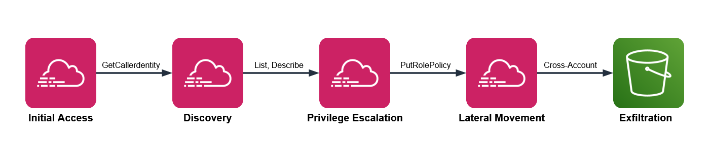
Multi-stage attacks move through five phases, and each phase leaves a signal in a different service. These signals surface across three log sources: CloudTrail, which records API activity in your account; Amazon VPC Flow Logs, which capture network connection metadata; and Amazon Route 53 Resolver query logs, which record DNS queries from your VPCs.

  • Initial access – Stolen credentials reach your environment. CloudTrail records GetCallerIdentity, GetSessionToken, or AssumeRole from an unfamiliar source.
  • Discovery – The threat actor enumerates with List, Describe, and Get calls, often triggering AccessDenied responses.
  • Privilege escalation – The threat actor chains roles or edits policies. CloudTrail records AssumeRole sequences, PutRolePolicy, or CreateAccessKey.
  • Lateral movement – The threat actor moves across accounts or AWS Regions, assuming roles and creating resources in unfamiliar places.
  • Exfiltration – Data leaves through GetObject calls at scale, large outbound transfers in VPC Flow Logs, and DNS queries in Route 53 Resolver query logs to recently registered domains.

Figure 1 shows the five attack phases mapped to the AWS log source that records each one.

Figure 1: Attack chain mapped to AWS services

Figure 1: Attack chain mapped to AWS services

GuardDuty Extended Threat Detection watches this chain for universal patterns. The four patterns that follow add the dimension you supply: your business context.

Pattern one: Sensitive data access by an unexpected principal

Your data classification and access norms drive this detection. One bucket holds customer records, another holds public web assets, and you know which principals have a reason to read the customer records, which are sensitive. Encode that knowledge and an ordinary looking read turns into something worth chasing.

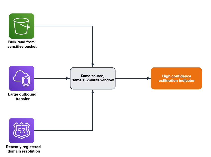
Three signals converge here. CloudTrail shows GetObject at volume on a bucket you’ve classified as sensitive. The principal isn’t on your list of expected readers for that bucket. And VPC Flow Logs show a large outbound transfer from the same source in the same window, while DNS query logs show a recently registered destination domain, which together increase your confidence that there’s a potential threat.

CloudTrail management events don’t record GetObject. You must turn on CloudTrail data events for the buckets you care about to capture GetObject. Many teams miss GetObject because data events weren’t enabled on the relevant buckets.

This query shows bulk reads on a sensitive bucket, grouped by principal. Run it in CloudWatch Logs Insights with your CloudTrail log group selected.

fields @timestamp, userIdentity.arn, requestParameters.bucketName
| filter eventSource = "s3.amazonaws.com" and eventName = "GetObject"
| filter requestParameters.bucketName = "your-sensitive-bucket"
| stats count(*) as objectReads,
        count_distinct(requestParameters.key) as distinctObjects
        by userIdentity.arn, bin(10m)
| filter objectReads > 100
| sort objectReads desc

The threshold of 100 is a placeholder. Run the query over a week of normal activity, find the ninety-fifth percentile read count for that bucket, and set the threshold above it. Then check each principal the query returns against your expected reader list. A principal that isn’t on the list, reading at volume, is the result to investigate.

To corroborate, look for a matching outbound transfer. Switch the log group selector to your VPC Flow Logs log group and run this.

fields @timestamp, srcAddr, dstAddr, bytes
| filter action = "ACCEPT"
# exclude RFC 1918 private ranges so only external destinations remain
| filter dstAddr not like /^10\./
        and dstAddr not like /^192\.168\./
        and dstAddr not like /^172\.(1[6-9]|2[0-9]|3[0-1])\./
| stats sum(bytes) as totalBytes by srcAddr, dstAddr, bin(10m)
| filter totalBytes > 1000000000
| sort totalBytes desc

The Amazon S3 query returns a principal, and the Flow Logs query works on IP addresses, so you translate one into the other. The worked example later in this post covers that translation in full.

Picture an analytics role that reads a reporting bucket all day. One afternoon, it reads a thousand objects from your customer records bucket instead. GuardDuty stays quiet, because an authenticated role making valid GetObject calls isn’t suspicious anywhere else. Your query flags it, because that role isn’t on the expected reader list for that bucket. The classification you applied is what turns silence into a signal.

Figure 2 shows a bulk read from a sensitive bucket in CloudTrail, a large outbound transfer in VPC Flow Logs, and a young domain resolution in Route 53 Resolver logs.

Figure 2: Three signals converging within a single time window to indicate exfiltration

Figure 2: Three signals converging within a single time window to indicate exfiltration

Pattern two: A role chain that crosses your access policy

Picture a deployment that assumes one role to build, then a second to release. For one principal, that two-hop AssumeRole chain is routine; for a different principal it’s a policy violation. This pattern relies on your trust topology—the chains your organization permits—so put that knowledge in the query.

This pattern needs three conditions:

  • CloudTrail shows several AssumeRole calls from the same source inside a short window
  • The chain ends in a sensitive action such as CreateAccessKey, PutRolePolicy, or AttachUserPolicy
  • The starting identity isn’t one your policy expects to run that chain

In CloudWatch Logs Insights, select your CloudTrail log group and run this query, which surfaces chains of two or more hops.

fields @timestamp, userIdentity.arn, requestParameters.roleArn, sourceIPAddress
| filter eventName = "AssumeRole"
| stats count(*) as assumeCount,
        count_distinct(requestParameters.roleArn) as rolesAssumed
        by sourceIPAddress, bin(5m)
| filter assumeCount >= 2 and rolesAssumed >= 2
| sort assumeCount desc

Two hops is the minimum for a chain; raise the count if your environment chains roles often. Your deployment pipeline probably assumes several roles an hour, as do AWS service principals such as AWS Security Hub. Exclude the identities you expect to see assuming multiple roles, including your pipeline role and known AWS service principals. What’s left is the set to investigate, such as a person assuming several roles at an odd hour and ending in a new access key. Treat that distinction as data: list the identities and actions you consider normal, and review the chains that fall outside the list.

Pattern three: An encryption key used outside its owning workload

Resource ownership is the signal here. A given AWS Key Management Service (AWS KMS) key creates and controls the encryption keys for a workload, and a single key should serve a single workload, such as a payments service. A Decrypt call against it is a valid, authorized API action, so nothing about the call itself looks wrong. The ownership rule you set is what makes another principal’s use of the key worth a second look.

This pattern applies only to customer-managed keys scoped to one workload. It doesn’t apply to AWS-managed keys (alias/aws/*) or to customer-managed keys intentionally shared across services. Confirm single-workload intent from the key policy’s Principal block before deploying this rule.

Two conditions indicate misuse:

  • CloudTrail shows Decrypt or GenerateDataKey calls on a key that’s tied to one workload
  • The calling principal isn’t the role that owns that workload

Against your CloudTrail log group, run this query to list the principals that called a specific key.

fields @timestamp, userIdentity.arn, eventName
| filter eventSource = "kms.amazonaws.com"
| filter eventName in ["Decrypt", "GenerateDataKey", "Encrypt"]
| filter resources.0.ARN = "arn:aws:kms:region:account-id:key/your-key-id"
| stats count(*) as keyUses by userIdentity.arn, eventName
| sort keyUses desc

Compare what comes back against the one workload role you expect. A principal you don’t recognize on that key is the signal. Because key misuse is an early move in data theft, this correlation catches activity that only your ownership knowledge can flag.

Consider a key that wraps your payments database. The payments service role calls it in normal operation, and nothing else should. If a developer role or a freshly created role runs Decrypt against it, the call succeeds and reads as ordinary in isolation. The reason it matters is the ownership rule you hold in your head and now state in this query.

Pattern four: A privileged action outside your change window

Start with the query, then read what it means.

fields @timestamp, userIdentity.arn, eventName, sourceIPAddress
| filter eventName in ["PutRolePolicy", "AttachRolePolicy",
        "CreateAccessKey", "AuthorizeSecurityGroupIngress", "PutBucketPolicy"]
| stats count(*) as sensitiveChanges by userIdentity.arn, eventName, sourceIPAddress
| sort sensitiveChanges desc

Run it against your CloudTrail log group, scoped to your off-hours window when you schedule it, so it returns only activity outside the change window. Your change process defines what normal looks like here: production security and identity changes flow through a pipeline during defined hours, run by a known actor. A console-driven policy change at 2:00 AM, made by a person rather than the pipeline, doesn’t fit those expectations. The signal is a sensitive change such as PutRolePolicy or AuthorizeSecurityGroupIngress, made outside the window, by a person rather than your pipeline role.

Exclude the actors you expect, such as your deployment pipeline role, your patch automation role, and AWS service principals like AWS CloudFormation and AWS Systems Manager. What remains is privileged change made outside your process, which is both what an attacker does to establish persistence and what your own change discipline says shouldn’t happen.

Your pipeline might open security group rules during a deployment every weekday afternoon. A person opening a security group rule at midnight on a weekend is the same API call carrying a very different meaning. The schedule and the actor, both facts you define, are what separate the two.

Build your first correlation rule

The following walkthrough uses pattern one as a complete example. The other three patterns follow the same design with their own queries.

Prerequisites

These prerequisites feed the queries in this walkthrough. Confirm each one before you start:

  • A CloudTrail trail logging management events to a CloudWatch Logs log group
  • CloudTrail data events enabled for your sensitive S3 buckets
  • GuardDuty enabled, with its protection plans and Extended Threat Detection
  • VPC Flow Logs on for your production VPCs
  • Amazon Route 53 Resolver query logging on

CloudTrail, GuardDuty, VPC Flow Logs, and Route 53 Resolver query logging provide the raw signals that your correlations connect. Without them, the queries in this post return empty results.

Step 1: Record the bucket and its expected readers

Choose one sensitive bucket to monitor, and write down the principals allowed to read it. Store the list where your automation can reach it, such as a configuration file in version control or an Amazon DynamoDB table (a managed NoSQL database).

{
  "customer-records-prod": [
    "arn:aws:iam::123456789012:role/AnalyticsPipeline",
    "arn:aws:iam::123456789012:role/ComplianceAudit"
  ],
  "financial-data-archive": [
    "arn:aws:iam::123456789012:role/FinanceReporting"
  ]
}

This example hardcodes the list for simplicity. In production, load it from a DynamoDB table or Parameter Store so you can update it without redeploying.

Step 2: Baseline before you set a threshold

Run the pattern one query over one week of normal activity. Find the 95th percentile read count for the bucket and use a value greater than that as your alert threshold. This step keeps legitimate high-volume access from generating false positives later.

Set the THRESHOLD_READS environment variable to this value when you configure the function in Step 5.

Step 3: Run the access query

In the CloudWatch console:

  1. Choose Logs, then choose Logs Insights.
  2. In the Select log group(s) dropdown, select your CloudTrail log group.
  3. Set the time range to 3h (the last three hours).
  4. In the query editor, paste the pattern one query.
  5. Replace your-sensitive-bucket with your bucket name.
  6. Choose Run query.
  7. Review the principals in the results table.
  8. Compare each principal against your expected reader list from step 1, and flag any that are not on it.

Each result includes a principal that step 4 translates into an IP address.

Step 4: Correlate with network activity

CloudTrail logs actions by AWS Identity and Access Management (IAM) principal, while VPC Flow Logs record traffic by IP address. To connect the two signals, translate the principal into its address.

For a role attached to an Amazon Elastic Compute Cloud (Amazon EC2) instance, the userIdentity.principalId field includes the instance ID after the colon, in the form AROAEXAMPLE:i-1234567890abcdef0. Copy the instance ID and look up its private IP address.

aws ec2 describe-instances \
  --instance-ids i-1234567890abcdef0 \
  --query "Reservations[0].Instances[0].PrivateIpAddress" \
  --output text

Other compute types differ. A VPC-connected AWS Lambda function sends traffic through elastic network interfaces in your subnets, so correlate on those interface addresses. An Amazon Elastic Container Service (Amazon ECS) task records its network interface in task metadata. For a plain assumed-role session with no instance behind it, the sourceIPAddress field in CloudTrail already holds the caller’s address, so you correlate on it directly.

Run the Flow Logs query from pattern one, filtering srcAddr to that address within 10 minutes of the Amazon S3 read timestamp. A match places the same source behind both the sensitive read and a large external transfer in one window. CloudTrail events reach CloudWatch Logs 5–15 minutes after the API call, so correlate on eventTime rather than query time. Query a wider lookback than your correlation window: for example, look back 30 to 60 minutes but correlate on a 10-minute eventTime window. Steps 3 and 4 are manual validation; step 5 automates them.

Figure 2 shows DNS resolution as a third corroborating signal. This walkthrough implements the CloudTrail and VPC Flow Logs correlation. To add DNS, apply the same run_query() pattern against your Route 53 Resolver query log group.

Step 5: Automate the check

Move the query into a Lambda function (serverless compute that runs your code without a server to manage), send results to a notification channel, and schedule regular runs. Work through the following sub-procedures.

To create the notification channel

  1. Open the Amazon Simple Notification Service (Amazon SNS) console. Amazon SNS is a managed messaging service that delivers notifications to subscribers.
  2. In the navigation pane, choose Topics.
  3. Choose Create topic.
  4. For Type, select Standard.
  5. For Name, enter security-correlation-alerts.
  6. Choose Create topic.
  7. Note the topic Amazon Resource Name (ARN) at the top of the topic details page. You will use it in the function.
  8. Choose Create subscription.
  9. For Protocol, select Email.
  10. For Endpoint, enter your email address or incident management endpoint.
  11. Choose Create subscription, then confirm the subscription from the email AWS sends.

To create the EventBridge Scheduler execution role

The schedule needs a role that lets it invoke your function, and its trust policy needs conditions that pin the role to the schedule you own. Without those conditions, another account with access to the scheduler service could theoretically call this role; a class of misuse known as the confused deputy problem.

1. Create a trust policy file named scheduler-trust-policy.json.

{
  "Version": "2012-10-17",
  "Statement": [
    {
      "Effect": "Allow",
      "Principal": { "Service": "scheduler.amazonaws.com" },
      "Action": "sts:AssumeRole",
      "Condition": {
        "StringEquals": {
          "aws:SourceAccount": "ACCOUNT-ID"
        },
        "ArnLike": {
          "aws:SourceArn": "arn:aws:scheduler:REGION:ACCOUNT-ID:schedule/*/s3-access-correlation-hourly"
        }
      }
    }
  ]
}

2. Create the role, then attach permission to invoke the function. Scope Resource to the specific function ARN so this role can’t invoke anything else.

aws iam create-role \
  --role-name EventBridgeSchedulerRole \
  --assume-role-policy-document file://scheduler-trust-policy.json

aws iam put-role-policy \
  --role-name EventBridgeSchedulerRole \
  --policy-name LambdaInvokePolicy \
  --policy-document '{
    "Version": "2012-10-17",
    "Statement": [
      {
        "Effect": "Allow",
        "Action": "lambda:InvokeFunction",
        "Resource": "arn:aws:lambda:REGION:ACCOUNT-ID:function:CorrelationFunction"
      }
    ]
  }'

When you create the function, Lambda automatically creates an execution role. You will attach the permissions this function needs to that role in a later step.

To deploy the correlation function

  1. Open the Lambda console.
  2. Choose Create function.
  3. For Function name, enter CorrelationFunction.
  4. For Runtime, select the latest Python runtime.
  5. Choose Create function.
  6. On the Code tab, replace the default code with the following function, then choose Deploy.
import os
import time
import logging
import boto3
from botocore.exceptions import ClientError

logger = logging.getLogger()
logger.setLevel(logging.INFO)

logs = boto3.client("logs")
sns = boto3.client("sns")
ec2 = boto3.client("ec2")

CLOUDTRAIL_LOG_GROUP = os.environ["CLOUDTRAIL_LOG_GROUP"]
FLOWLOGS_LOG_GROUP = os.environ["FLOWLOGS_LOG_GROUP"]
SNS_TOPIC = os.environ["SNS_TOPIC_ARN"]
BUCKET = os.environ["SENSITIVE_BUCKET"]
THRESHOLD = int(os.environ.get("THRESHOLD_READS", "100"))

# Expected readers per bucket
EXPECTED_READERS = {
    "customer-records-prod": [
        "arn:aws:iam::123456789012:role/AnalyticsPipeline",
        "arn:aws:iam::123456789012:role/ComplianceAudit",
    ],
}


def run_query(log_group, query, start, end):
    """Start a Logs Insights query and wait for it to finish."""
    started = logs.start_query(
        logGroupName=log_group,
        startTime=start,
        endTime=end,
        queryString=query,
    )
    query_id = started["queryId"]
    while True:
        outcome = logs.get_query_results(queryId=query_id)
        if outcome["status"] in ("Complete", "Failed", "Cancelled"):
            break
        time.sleep(1)
    if outcome["status"] != "Complete":
        raise RuntimeError(f"Query did not complete: {outcome['status']}")
    return [{f["field"]: f["value"] for f in row} for row in outcome["results"]]


def private_ip_for_principal(principal_id):
    """Resolve an EC2 instance role principalId to its private IP."""
    if ":" not in principal_id:
        return None
    instance_id = principal_id.split(":", 1)[1]
    if not instance_id.startswith("i-"):
        return None
    reservations = ec2.describe_instances(InstanceIds=[instance_id])
    for reservation in reservations["Reservations"]:
        for instance in reservation["Instances"]:
            return instance.get("PrivateIpAddress")
    return None


def egress_bytes(src_addr, start, end):
    """Sum external egress bytes for one source address."""
    query = f"""
    fields srcAddr, dstAddr, bytes
    | filter action = "ACCEPT" and srcAddr = "{src_addr}"
    | filter dstAddr not like /^10\\./
            and dstAddr not like /^192\\.168\\./
            and dstAddr not like /^172\\.(1[6-9]|2[0-9]|3[0-1])\\./
    | stats sum(bytes) as totalBytes
    """
    rows = run_query(FLOWLOGS_LOG_GROUP, query, start, end)
    if rows and rows[0].get("totalBytes"):
        return int(rows[0]["totalBytes"])
    return 0


def lambda_handler(event, context):
    try:
        # 1-hour lookback absorbs CloudTrail's 5-15 min delivery latency;
        # correlation happens on eventTime via 10-min bins in the query below.
        end = int(time.time())
        start = end - 3600  # 1 hour lookback
        allowed = EXPECTED_READERS.get(BUCKET, [])

        access_query = f"""
        fields userIdentity.arn, userIdentity.principalId
        | filter eventSource = "s3.amazonaws.com" and eventName = "GetObject"
        | filter requestParameters.bucketName = "{BUCKET}"
        | stats count(*) as objectReads
                by userIdentity.arn, userIdentity.principalId, bin(10m)
        | filter objectReads > {THRESHOLD}
        """

        for row in run_query(CLOUDTRAIL_LOG_GROUP, access_query, start, end):
            principal = row.get("userIdentity.arn")
            if not principal or principal in allowed:
                continue

            message = (
                f"Principal {principal} read {row.get('objectReads')} "
                f"objects from {BUCKET}."
            )

            ip = private_ip_for_principal(row.get("userIdentity.principalId", ""))
            if ip and egress_bytes(ip, start, end) > 1_000_000_000:
                message += (
                    f" The same source ({ip}) also sent a large volume of "
                    f"data to external destinations in the same window."
                )

            sns.publish(
                TopicArn=SNS_TOPIC,
                Subject="Unexpected S3 access detected",
                Message=message,
            )
    except ClientError as error:
        logger.error(f"AWS API error: {error}")
        raise
    except Exception as error:
        logger.error(f"Unexpected error: {error}")
        raise
    finally:
        logger.info("Correlation check completed")

  1. On the Configuration tab, choose General configuration, then choose Edit. Set Timeout to 5 minutes (300 seconds). CloudWatch Logs Insights queries run asynchronously and can take 30 to 60 seconds against large log groups. Choose Save.
  2. On the Configuration tab, choose Environment variables, then choose Edit, and add CLOUDTRAIL_LOG_GROUP, FLOWLOGS_LOG_GROUP, SNS_TOPIC_ARN, SENSITIVE_BUCKET, and THRESHOLD_READS.
  3. On the Configuration tab, choose Permissions, open the execution role, and attach the following least-privilege policy.
{
  "Version": "2012-10-17",
  "Statement": [
    {
      "Effect": "Allow",
      "Action": ["logs:StartQuery", "logs:GetQueryResults"],
      "Resource": [
        "arn:aws:logs:REGION:ACCOUNT-ID:log-group:aws-cloudtrail-logs-my-trail:*",
        "arn:aws:logs:REGION:ACCOUNT-ID:log-group:vpc-flow-logs:*"
      ]
    },
    {
      "Effect": "Allow",
      "Action": "ec2:DescribeInstances",
      "Resource": "*"
    },
    {
      "Effect": "Allow",
      "Action": "sns:Publish",
      "Resource": "arn:aws:sns:REGION:ACCOUNT-ID:security-correlation-alerts"
    }
  ]
}

Replace REGION, ACCOUNT-ID, and the log-group names with your values. The ec2:DescribeInstances action doesn’t support resource-level permissions, so Resource: "*" is required for that statement; the other statements are scoped to specific ARNs.

To schedule automated runs

Amazon EventBridge (a serverless event bus that connects applications using events) runs targets on a schedule. Create one from the command line, using the role you made earlier.

aws scheduler create-schedule \
  --name s3-access-correlation-hourly \
  --schedule-expression "rate(1 hour)" \
  --target "Arn=arn:aws:lambda:REGION:ACCOUNT-ID:function:CorrelationFunction,RoleArn=arn:aws:iam::ACCOUNT-ID:role/EventBridgeSchedulerRole" \
  --flexible-time-window "Mode=OFF"

Step 6: Add enrichment context (optional)

Enrichment cuts triage time by adding an independent signal, but it isn’t required for the correlation to work. This step adds costs. You pay your geolocation provider for API calls, and the additional Lambda execution time increases your Lambda charges. To add IP geolocation, sign up for a geolocation API, add this function to the code, and call it where the handler resolves an IP.

import urllib.request
import json

def geo_context(ip_address):
    """Enrich an IP address with geolocation data from your provider."""
    try:
        url = f"https://your-geolocation-api.example/json/{ip_address}"
        with urllib.request.urlopen(url, timeout=5) as response:
            data = json.load(response)
        return {
            "country": data.get("country_name"),
            "city": data.get("city"),
            "org": data.get("org"),
        }
    except Exception as error:
        logger.warning(f"Geolocation lookup failed for {ip_address}: {error}")
        return None

Inside the handler’s loop, after you resolve ip, append the location to the alert.

            if ip:
                geo = geo_context(ip)
                if geo:
                    message += (
                        f" Source location: {geo['city']}, "
                        f"{geo['country']} ({geo['org']})."
                    )

Step 7: Scale to additional patterns and accounts

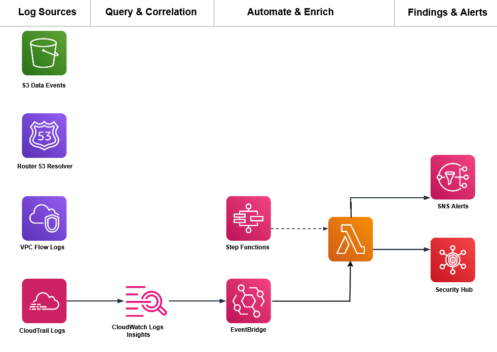
As your library grows, move the logic into automated pipelines with EventBridge, Lambda, and AWS Step Functions (a serverless orchestration service that coordinates multiple services into workflows), and surface correlations next to findings in Security Hub. For cross-service correlation at scale, CloudWatch unified data and telemetry capabilities can convert security and compliance data into the OCSF format and let you query sources such as CloudTrail, VPC Flow Logs, and DNS logs from one interface. Security Lake with Athena is a strong option for long-term analysis. Choose the endpoint that fits your retention and query needs.

Figure 3 shows a correlation pipeline built on AWS services including EventBridge, Lambda, Step Functions, and AWS Security Hub. The pipeline runs from data sources through scheduled queries and enrichment to automated response and centralized visibility.

Figure 3: A correlation pipeline built on AWS services

Figure 3: A correlation pipeline built on AWS services

Conclusion

You now have four correlation patterns that layer your business context on top of GuardDuty Extended Threat Detection to catch attacks specific to your environment. A few principles carry across every correlation you build.

  • Identity is your primary correlation key: Track the same principal across services.
  • Time windows matter, but they depend on the attack: Events minutes apart are usually related for fast, automated sequences; the ten-minute bins here work for that pattern. Slow or manual reconnaissance can stretch across hours or days, so widen the window when the pattern is deliberate rather than automated.
  • Context is what you add: Your data classification, access norms, resource ownership, and change windows are signals you bring to detection.
  • Start with one rule: A single well-tuned correlation catches more significant activity than a wall of uncorrelated alerts.

GuardDuty Extended Threat Detection handles the multi-stage patterns common across customers. The correlations in this post add the layer that only your business context can supply. Start with one pattern this week, validate it against your own traffic, and add the next pattern after the first proves reliable.

Have you built correlation rules for patterns not covered here? Share your experience in the Comments section below.

Further reading

 

Nisha Kashyap

Nisha Kashyap

Nisha Kashyap is a Senior Support Security Engineer at AWS. She works on threat detection and security operations, helping customers investigate security events and build detection that connects signals across AWS services and reflects their own environment.

Streamline your GitHub journey with AWS CodePipeline and AWS DevOps Agent

Post Syndicated from Anjani Reddy original https://aws.amazon.com/blogs/devops/streamline-your-github-journey-with-aws-codepipeline-and-aws-devops-agent/

Introduction

When CI/CD deployment failures occur for GitHub hosted applications,  AWS DevOps Agent reduces the hours that Development and Site Reliability Engineering (SRE) teams typically spend manually investigating across multiple AWS services, logs, and pipeline stages. This process delays critical deployments and impacts software delivery velocity. This is especially true when teams need to correlate data between GitHub commit histories, AWS CodePipeline execution logs, and Amazon CloudWatch metrics. When continuous integration and continuous delivery (CI/CD) pipelines fail, engineers often find themselves context-switching between GitHub pull requests, code build logs, deployment artifacts, and downstream service health metrics. This process of identifying root causes can extend resolution time from minutes to hours, especially in multi-service architectures.

AWS DevOps Agent reduces this manual investigation by automatically correlating pipeline failures with specific code changes. Rather than spending hours manually tracing deployment failures through multiple systems, engineers can use AWS DevOps Agent to perform this correlation. It identifies which specific code changes caused pipeline failures and provides remediation guidance. The agent analyzes pipeline failures, correlates them with specific commits and pull requests, and identifies root causes across the deployment chain.

AWS CodePipeline combined with AWS DevOps Agent helps address this challenge by creating a streamlined path from GitHub repositories to AWS deployments. This solution reduces manual handoffs, reduces configuration complexity, and provides end-to-end visibility across the entire development lifecycle.

In this post, you learn how to integrate AWS DevOps Agent with your GitHub repositories to automatically correlate deployment failures with specific commits, providing root cause analysis and remediation steps across your entire CI/CD pipeline.

Solution overview 

Modern software delivery teams face a persistent challenge: when deployments fail, engineers spend valuable time manually correlating logs, tracing pipeline errors, and diagnosing root causes across disconnected tools. This reactive cycle slows recovery and increases mean time to resolution (MTTR). By integrating the AWS DevOps Agent with GitHub, AWS CodePipeline, Amazon CloudWatch, and AWS Lambda, teams can shift from manual triage to automated incident investigation, directly within their existing GitHub-based workflows.

This solution integrates AWS DevOps Agent with GitHub to automate deployment failure investigation. The following sections explain the architecture and operational benefits.

How it works​ 

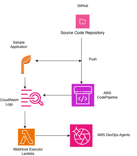
The architecture creates an automated monitoring and remediation flow that monitors your deployment pipeline and responds to issues. Your source code resides in a GitHub repository, and AWS CodePipeline orchestrates the build, test, and deployment stages. Amazon CloudWatch continuously monitors pipeline execution metrics and logs and generates alarms when it detects anomalies or failures, such as failed build stages, deployment rollbacks, or threshold breaches in downstream application of health metrics. When a failure occurs, it generates an error metric in CloudWatch. The CloudWatch Alarm detects this error and transitions to an ALARM state, which directly invokes the WebHook Executor Lambda. The WebHook Executor then sends an authenticated HTTP POST request to DevOps Agent, which receives the incident and begins an investigation.

Webhook integration acts as the bridge between the Amazon CloudWatch, the monitoring layer. Lambda parses the alarm payload and extracts contextual metadata and then invokes the DevOps Agent with a structured investigation request.

Integration with Operational Excellence

This solution directly supports the AWS Well-Architected Framework’s Operational Excellence pillar by automating the investigation process and reducing the MTTR. The investigation capability of AWS DevOps Agent aligns with AWS Incident Detection and Response (IDR) best practices, helping teams to detect, diagnose, and develop mitigation plans for pipeline failures faster while maintaining a full audit trail of agent actions and findings. This creates a delivery pipeline that accelerates resolution workflows through automated diagnostics and actionable remediation recommendations, keeping deployments moving and engineering teams focused on building rather than firefighting.

Architecture diagram showing GitHub repository connected to AWS CodePipeline, CloudWatch, Lambda, and DevOps Agent in an automated investigation flow 

Figure 1: GitHub and DevOps Agent integration

Prerequisites 

For this walkthrough, you should have access to and understanding of the following:

  •  An AWS account with permissions to create AWS Identity and Access Management (IAM) roles:
    1. Agent Space role – for basic service operations.
    2. Agent Space web app role – for using the Agent Space web app functionality.
    3. (Optional) Secondary source account roles if monitoring multiple AWS accounts. Refer to the DevOps Agent user guide for the details on setting up these roles.
  • A GitHub account:
    1. You have a GitHub account with administrative permissions for your repositories, or an organization you belong to.
    2. Your repositories contain code that deploys to AWS resources you want to monitor.
    3. You have identified the GitHub repositories you want AWS DevOps agent to access.
  • Access to register DevOps Agent with your GitHub Account or Organization.
  • CloudWatch monitoring enabled for your application.

​​Implementation steps​ 

Note: For this blog we used a sample application  from the AWS-samples.

  1. ​​Create an AWS DevOps Agent Space and configure the webhook​
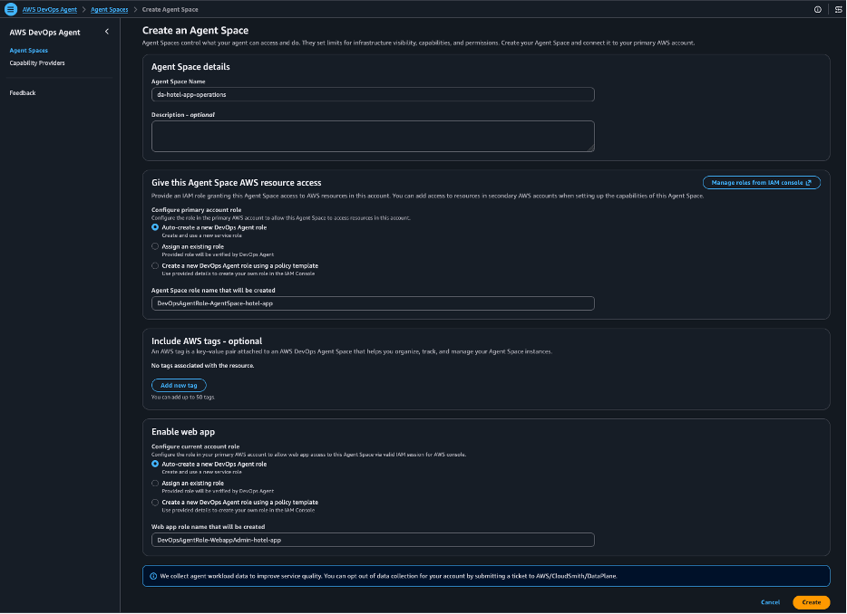
    The first step is to create a dedicated Agent Space that serves as the central hub for your automated investigation workflow. The Agent Space connects your monitoring infrastructure to the DevOps Agent’s analysis capabilities.
    Create the DevOps Agent space by following the steps outlined in the Getting Started with AWS DevOps Agent guide Navigate to the DevOps Agent console.
    Create an Agent Space named after your application (for example, `myhotelapp`)
    1) “Auto-create both IAM roles”.
    2) “Edit the role names to be descriptive (for example, DevOpsAgentRole-AgentSpace-hotel-app and DevOpsAgentRole-WebappAdmin-hotel-app)”
Screenshot of AWS DevOps Agent console showing the Agent Space creation interface with IAM role configuration options

Figure 2: Agent Spaces Screen

On the Capabilities tab, generate a webhook and save the credentials

Store the webhook credentials in AWS Secrets Manager:

```bash

aws secretsmanager create-secret \

--name devops-agent-webhook-credentials \

--secret-string '{"webhookUrl":"YOUR-WEBHOOK-URL","webhookSecret":"YOUR-WEBHOOK-SECRET"}' \

--region us-east-1

```

2. Configure GitHub integration with your AgentSpace

With your Agent Space created and webhook configured, the next step is to connect your GitHub repositories. This integration allows the DevOps Agent to access commit histories, pull request data, and code changes when investigating pipeline failures.

To configure GitHub integration with your AgentSpace:
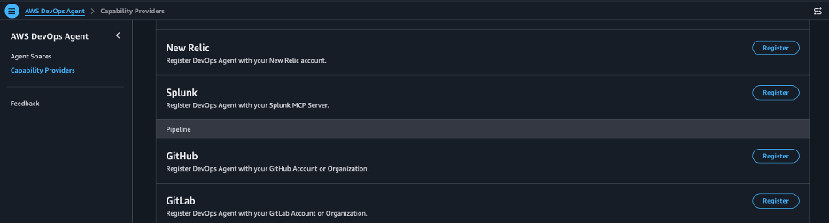
1. From the Capabilities tab within your configured AgentSpace, navigate to the GitHub Configuration section and choose “Register”

Screenshot of the GitHub Configuration section in the AgentSpace Capabilities tab showing the Register button

Figure 3: Capability Providers

2.     Your GitHub repositories will be listed with their connection status.

3.     To connect to a repository, verify that the Status shows “Ready to connect” and choose the + button in the Actions column.

4.     Upon successful connection, the Status updates to ‘Connected’.

To automatically trigger AWS DevOps Agent investigations via Webhook when a CloudWatch enters the ALARM state, you can refer to sample-aws-devops-agent-cloudwatch and build based on your use case.

3. Troubleshooting application deployment 5XX errors with CloudWatch and AWS DevOps Agent

When your application encounters 5XX errors during deployment, CloudWatch alarms detect the anomaly and trigger the DevOps Agent investigation workflow. The following dashboard shows the alarm state that initiates the automated investigation process.

Screenshot of CloudWatch dashboard displaying alarm metrics triggered by application 5XX errors

Figure 4: CloudWatch Dashboard

4. Resolving deployment/build errors during CI/CD deployment

The following use cases demonstrate how AWS DevOps Agent investigates and resolves common CI/CD pipeline failures. Each scenario walks through the failure trigger, the automated investigation, and the remediation guidance that the agent provides

Use case 1: Push a code change that introduces an invalid DynamoDB table name

Simulate: Push a code change that breaks the DynamoDB table name — e.g., change DYNAMODB_TABLE_NAME env var but don’t update CloudFormation to make the CodePipeline unit testing fail

A – dynamodb_table: process.env.DYNAMODB_TABLE_NAME || “Rooms”,

B + dynamodb_table: “HotelRooms”

The CodePipeline triggers 5xx alarms and the webhook triggers a DevOps Agent investigation.

DevOps Agent analyzes the 500 errors in relation to the configuration change, identifies the invalid DynamoDB endpoint, and shows the timeline: configuration update → service redeployment → requests fail with connection errors.

Screenshot of CodePipeline execution view showing a failed unit test stage highlighted in red

Figure 5: Unit test failed for the CodePipeline

Use case 2: Identifying dependency resolution failures from bad commits

1. Navigate to `package.json`

2. Change any dependency name to something invalid — for example, change `”express”` to `”expresss”` (extra ‘s’)

3. Commit the change directly to `main`

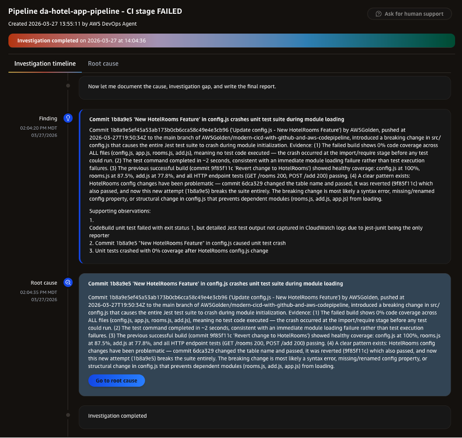
CodePipeline detects the push and starts a new execution. The CI stage runs `npm install`, which fails because the misspelled package doesn’t exist. The Amazon EventBridge rule catches the stage failure and invokes the webhook executor Lambda, which triggers a DevOps Agent investigation.

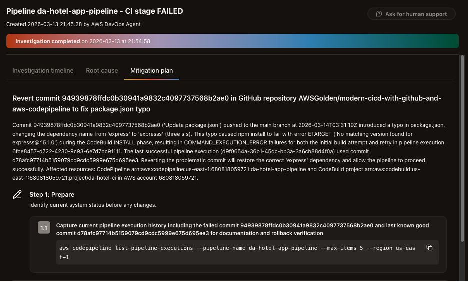
In the DevOps Agent console, select your Agent Space, then choose Operator access to open the web app.  Navigate to the Incident Response tab to view the new investigation.

Screenshot of DevOps Agent showing the first step of the mitigation plan identifying the root cause

Figure 6: Mitigation plan step1

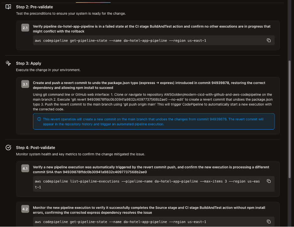
Screenshot of DevOps Agent showing steps 2 through 4 of the mitigation plan with remediation commands

Figure 7: Mitigation plan steps 2-4

DevOps Agent investigates the pipeline failure, examines the CodeBuild logs showing the `npm install` error, and correlates it with the recent commit to the repository. It identifies the root cause as a dependency resolution failure introduced by the latest code change.

Clean up

This walkthrough creates AWS resources that incur charges, including AWS DevOps Agent (pay-per-use), Lambda functions, CodePipeline executions, CloudWatch alarms, and Secrets Manager secrets. Follow the cleanup steps when finished to avoid ongoing charges.

1. Delete the Secrets Manager secret devops-agent-webhook-credentials using: aws secretsmanager delete-secret –secret-id devops-agent-webhook-credentials –region us-east-1

2. Delete your Agent Space from the AWS DevOps Agent console

3. Remove the GitHub pipeline connection from your settings.

4. Delete the IAM roles created for the Agent Space.

5. Delete the Lambda function, EventBridge rule, and CloudWatch alarms created for webhook integration.

6. (Optional) If you created additional source account roles, remove those as well.

Conclusion

The AWS DevOps Agent integration with GitHub fundamentally transforms how engineering teams approach CI/CD reliability by shifting from reactive troubleshooting to proactive incident prevention. By autonomously correlating CodePipeline failures with specific GitHub commits, analyzing root causes across the deployment chain, and providing intelligent remediation recommendations, this solution reduces mean time to resolution from hours to minutes while maintaining the human oversight necessary for production environments.

Organizations implementing this integration gain a resilient software delivery pipeline that combines the collaborative strengths of GitHub source control with AWS’s intelligent automation capabilities. This helps teams maintain deployment velocity, strengthen operational excellence, and focus engineering effort on innovation rather than incident response.

AWS CodePipeline, Amazon CloudWatch, AWS Lambda, and the AWS DevOps Agent integrate natively to provide end-to-end visibility and autonomous investigation capabilities. Together, they accelerate recovery workflows, reduce operational friction, and build the foundation for continuous delivery at scale.

About authors

Anjani Reddy

Anjani is a Sr. Solutions Architect at AWS. She works with Enterprise customers to provide operational guidance to innovate and build a secure, scalable cloud on the AWS platform. Outside of work, she is an Indian classical & salsa dancer, loves to travel and Volunteers for American Red Cross & Hands on Atlanta.

Jared Thompson
Jared Thompson is a Senior Technical Account Manager at AWS, where he partners with strategic enterprise customers to optimize cloud operations and accelerate AI/ML workloads at scale. Jared specializes in GPU-accelerated computing, capacity planning, and cloud observability, with a passion for turning complex infrastructure challenges into automated, self-healing systems. He is a recipient of the AWS Golden Jacket award and when not at work, he can be found on a cruise ship.

Aneesh Varghese is a Senior Technical Account Manager at AWS with more than 19 years of Information Technology industry experience. Aneesh supports enterprise customers in cost optimization strategies, Cloud operations, MLOps, providing advocacy and strategic technical guidance to help plan and build solutions using AWS best practices. Outside of work, Aneesh likes to spend time with family, play Basketball and Badminton.

AWS Weekly Roundup: Price reduction of GPT models in Bedrock, CloudWatch managed collectors for Prometheus metrics, and more (August 3, 2026)

Post Syndicated from Micah Walter original https://aws.amazon.com/blogs/aws/aws-weekly-roundup-price-reduction-of-gpt-models-in-bedrock-cloudwatch-managed-collectors-for-prometheus-metrics-and-more-august-3-2026/

Last week I had the joy of participating in Amazon’s “Bring Your Kids to Work Day” with my 7 year old son. We commuted together into the New York City office, his first real rush hour train ride, and spent the day exploring how Amazon uses AI, machine learning, and robotics to deliver packages to customers all over the world. Watching his eyes light up as he saw robots navigating a fulfillment center reminded me why so many of us got into technology in the first place. There’s nothing quite like seeing that sense of wonder when something complex clicks.
That same energy carried into the week’s launches. We’ve got updates across AI pricing, observability, multicloud networking, and data management. Let’s dive in.

Headlines
Amazon Bedrock announces up to 80% lower prices for OpenAI GPT‑5.6 models – If you’re using OpenAI’s GPT‑5.6 family through Amazon Bedrock, your costs just dropped significantly. Effective July 30, on-demand inference prices for GPT‑5.6 Luna are reduced by 80%, while GPT‑5.6 Terra prices are reduced by 20%. Luna now costs $0.20 per million input tokens and $1.20 per million output tokens, making it one of the most affordable frontier-class models available. These price reductions apply automatically — no action required on your part. Read more

Last week’s launches
Here are some launches and updates from this past week that caught my attention:

  • Amazon CloudWatch announces managed Prometheus collectors – Amazon CloudWatch now supports collecting Prometheus metrics from your AWS infrastructure using fully managed collectors, enabling you to monitor Amazon EKS, Amazon EC2, Amazon ECS, Amazon MSK, and Amazon OpenSearch Service workloads without deploying or managing any agents. If you’ve been maintaining your own Prometheus scraping infrastructure, this removes a significant operational burden. Read more
  • AWS Interconnect — multicloud connectivity with Oracle Cloud Infrastructure is now generally available – AWS Interconnect is the first purpose-built multicloud connectivity product of its kind, allowing you to quickly provision resilient, scalable private connections between AWS and other cloud providers. With this GA launch for Oracle Cloud Infrastructure (OCI), you can establish private cross-cloud networking without traversing the public internet, making it easier to run multicloud architectures with the security and performance your workloads demand. Read more
  • AWS IAM Identity Center extends multi-Region support to Identity Center directory – You can now replicate IAM Identity Center from your primary AWS Region to additional Regions when using the Identity Center directory as your identity source. If IAM Identity Center is affected by a disruption in the primary Region, your users continue to have access to their AWS accounts using provisioned entitlements in additional Regions. This feature was previously available only for instances connected to external identity providers. Read more
  • Amazon S3 Tables now supports the Variant data type for Apache Iceberg V3 – Amazon S3 Tables adds support for the Variant data type, introduced in the Apache Iceberg V3 table format specification. Variant provides a high-performance, native solution for managing semi-structured data within your data lake — think IoT sensor data, application logs, and other schema-flexible payloads — without resorting to JSON blobs. Read more

Other AWS news
Here are some additional posts and resources that you might find interesting:

Upcoming AWS events
Check your calendar and sign up for upcoming AWS events:

  • AWS Summits – AWS Summits are free events that bring the cloud and AI community together to connect, learn, and explore the latest technologies. Browse the full calendar to find a Summit near you in the second half of 2026.
  • AWS Community Days – Community-led conferences where content is planned, sourced, and delivered by community leaders.

Join the AWS Builder Center to connect with builders, share solutions, and access content that supports your development. Browse here for upcoming AWS-led in-person and virtual events and developer-focused events.


That’s all for this week. Check back next Monday for another Weekly Roundup!

New: Enhanced AssetState dimension for AWS Outposts capacity metrics on Amazon CloudWatch

Post Syndicated from Rachel McElwaine original https://aws.amazon.com/blogs/compute/new-enhanced-assetstate-dimension-for-aws-outposts-capacity-metrics-on-amazon-cloudwatch/

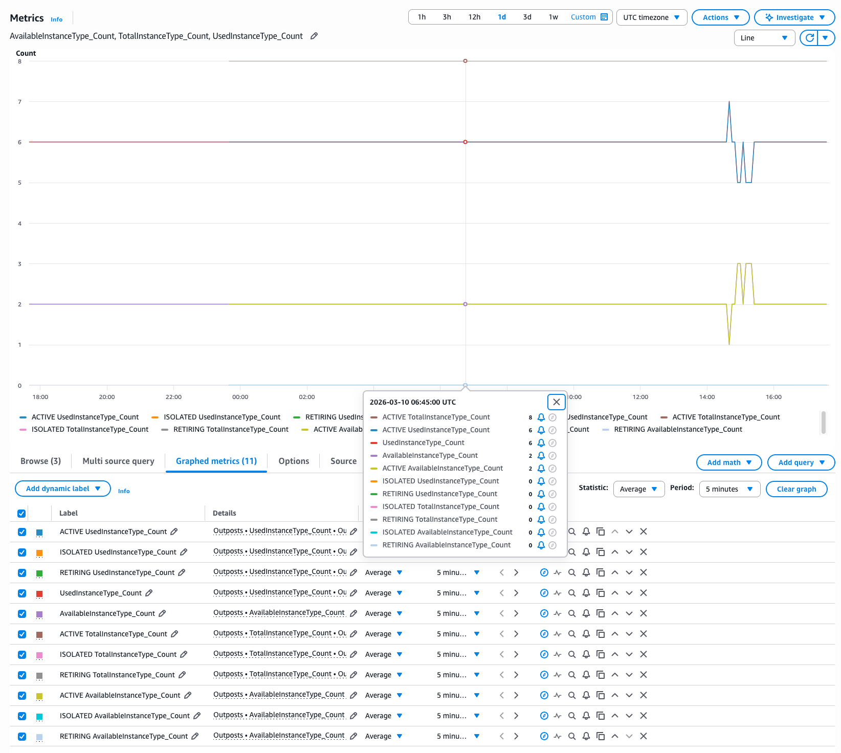
Today, we are releasing an expanded format of our Amazon CloudWatch dimensions for AWS Outposts capacity metrics. The existing CloudWatch metrics, AvailableInstanceType_Count, UsedInstanceType_Count, InstanceTypeCapacityAvailability, and InstanceTypeCapacityUtilization for Outposts, can now be grouped using the new AssetState dimension with values: Active, Isolated, or Retiring. In this post, we describe what’s changing and how you can use this dimension to improve your capacity monitoring.

What’s changing

Previously, an Outpost could be moved to one of these asset states following an AWS maintenance action, either by an on-site visit or by a remote network update. These state transitions are triggered by control plane operations and previously were not surfaced in customer-facing metrics. This could lead to incorrect or misleading capacity counts.

With this enhancement, you can group the metrics by the dimension to distinguish capacity between production-ready resources and capacity temporarily offline for maintenance.

Introducing the new AssetState dimension

This new dimension adds more visibility into the state of your first-generation and second-generation Outpost racks and servers. The values show the internal state of the AWS Outposts hardware and describe the current working state of the Outpost. These new values are:

  • ACTIVE – The Outpost is production-ready and can launch instances.
  • ISOLATED – The server or asset within the Outpost was taken offline and is temporarily unavailable.
  • RETIRING – The compute asset is not available for use. This state is used when a replacement part is needed.

The new AssetState dimension can be used for creating Amazon CloudWatch alarms for better monitoring, visibility, and alerting of AWS Outposts capacity.

Example metrics output

5 Server/Assets: 4 Active, 1 Isolated, 3 Active used, 1 Isolated used:

AvailableInstanceType_Count | i3en.metal-2tb | count = 1
AvailableInstanceType_Count | i3en.metal-2tb | ACTIVE | count = 1
AvailableInstanceType_Count | i3en.metal-2tb | ISOLATED | count = 0
AvailableInstanceType_Count | i3en.metal-2tb | RETIRING | count = 0

UsedInstanceType_Count | i3en.metal-2tb | count = 4
UsedInstanceType_Count | i3en.metal-2tb | ACTIVE | count = 3
UsedInstanceType_Count | i3en.metal-2tb | ISOLATED | count = 1
UsedInstanceType_Count | i3en.metal-2tb | RETIRING | count = 0

InstanceTypeCapacityAvailability | i3en.metal-2tb | 20%
InstanceTypeCapacityUtilization | i3en.metal-2tb | 80%

Figure 1: Amazon CloudWatch metrics with the AssetState dimension for AWS Outposts.

You can now accurately monitor your AWS Outposts capacity and set CloudWatch alarms that reflect available capacity with near real-time visibility.

Integration with CloudWatch on Outposts

This enhanced dimension is fully integrated with CloudWatch on Outposts, so you can monitor your local AWS Outposts infrastructure with the same observability tools you use in AWS Regions.

With the new AssetState dimension, you can create more precise CloudWatch alarms on your Outpost that trigger only on capacity status changes (ACTIVE/ISOLATED/RETIRING). This is particularly valuable if you run mission-critical workloads on Outposts and need accurate, real-time visibility into your on-premises capacity.

Availability

These new metrics are enabled by default and available to all AWS Outposts customers at no additional cost in all AWS Regions where AWS Outposts is offered.

Conclusion

The new AssetState dimension gives AWS Outposts customers clear visibility into the different hardware states of Active, Isolated, or Retiring. This visibility helps you maintain accurate capacity counts and create more precise CloudWatch alarms.

To learn more about CloudWatch metrics for AWS Outposts, refer to the Outposts monitoring documentation. For information about CloudWatch on Outposts and local monitoring capabilities, visit the CloudWatch on Outposts documentation.

How BigBasket uses the Iceberg based lakehouse architecture on AWS to power lightning-fast grocery delivery across India

Post Syndicated from Annie Mattoo original https://aws.amazon.com/blogs/big-data/how-bigbasket-uses-the-iceberg-based-lakehouse-architecture-on-aws-to-power-lightning-fast-grocery-delivery-across-india/

Delivering fresh groceries to millions of customers across India in a few minutes demands a radically modern data architecture and resilient processes to help the business make faster decisions. This is what BigBasket was able to achieve by building a lakehouse architecture on AWS.

In this post, we demonstrate how BigBasket implemented the lakehouse architecture on AWS, including their architecture decisions, implementation approach, and the measurable business results you can expect from a similar modernization. Whether you’re facing scalability challenges or planning your own lakehouse implementation, this blueprint provides actionable insights you can adapt for your organization.

About BigBasket

BigBasket (Innovative Retail Concepts Private Limited) is India’s largest online supermarket, serving millions of customers across over 60 cities. Founded in 2011, the company offers groceries, fresh produce, household items, and personal care products through its mobile app and website, operating subscription services (BBDaily) and quick commerce (bbnow). For BigBasket, the ability to deliver groceries on time isn’t only a competitive advantage. It’s the foundation of customer trust, where every minute counts.

However, rapid business growth brought significant operational challenges:

  • Inability to consistently meet on-time delivery adherence because of high order volumes, extended travel times, and more, directly impacting key metrics like on-time rate (OTR)-10 mins and OTR-15 mins.
  • Struggling to meet on-time delivery targets because of picking inefficiency, high order volumes, and extended travel times, directly impacting key metrics like OTR-10 mins and OTR-15 mins.
  • Delays in stock availability impacting vendor fill-rates, inter-distribution center orders, and warehouse operations.
  • Inaccurate stock forecasting for top-selling stock keeping units (SKUs), assortment variety, event SKUs, store capacity, and buying cycles.
  • Lower dark store productivity across picking, stacking, order processing, and goods receipt notes (GRN).

Behind these business challenges lay a fundamental technology problem: the existing data infrastructure couldn’t keep pace. The company experienced rapid store growth, expanding 4x in a short timeframe, which exposed several limitations within their existing data architecture that needed attention.

Understanding the technical bottlenecks

BigBasket’s initial architecture relied heavily on a single data warehouse built on Amazon Redshift to meet all reporting and dashboarding needs. While this traditional approach had served them well initially, several important limitations emerged:

  • Stale data: Extract, transform, load (ETL) pipelines delivered only day-old (D-1) data, making near real-time analysis impossible for dashboard requirements.
  • Extended recovery times: Pipeline failure recovery processes took several hours, causing significant delays in data availability for business users.
  • Schema rigidity: Schema changes in source databases frequently triggered pipeline failures because of a lack of schema evolution support.
  • Scalability constraints: The infrastructure struggled to handle the sudden load increase from 13,000 to over 35,000 transactions for reports and dashboards with more than 1,000 dataset refreshes.
  • Cost implications: Increasing data volumes demanded additional compute resources, driving up costs.

Diagram of the scalability and cost limitations of BigBasket’s legacy Amazon Redshift data warehouse

It became clear that the existing data infrastructure wasn’t able to meet the evolving business requirements and a redesign of their data architecture is needed.

Why lakehouse architecture?

A modern data lakehouse architecture addresses these issues with near real-time data processing, flexible schema evolution, and scalable analytics, capabilities necessary for fast-moving commerce operations. The lakehouse approach combines the flexibility and cost-effectiveness of data lakes with the performance and governance features of data warehouses, combining the strengths of both. The design of a data lakehouse provides interoperability across storage systems for combined analytics activities.

Solution overview

BigBasket partnered with AWS to implement a comprehensive lakehouse architecture using a combination of AWS native services and open-source technologies.

The following diagram shows an elaborated view of Bigbasket’s modernized architecture on AWS.

Detailed lakehouse data flow across bronze, silver, and gold medallion layers on AWS

Data ingestion: Enabling continuous replication

AWS Database Migration Service (AWS DMS) ingests data from online transaction processing (OLTP) databases running on Amazon Relational Database Service (Amazon RDS) into the lakehouse on AWS.

This method continuously replicates data with minimal latency, so your analytics reflect near real-time business operations.

Storage and governance: Building a solid foundation

The lakehouse is built on Amazon Simple Storage Service (Amazon S3) and Amazon Redshift, which serve as the centralized data lake and warehouse following a medallion architecture.

The architecture persists all analytical data using Apache Iceberg as the open table format. Iceberg provides a robust foundation for large-scale analytics with the following capabilities:

  • ACID transactions: Guarantees data consistency and correctness across concurrent read and write operations.
  • Time travel: Supports querying historical table versions for auditing, troubleshooting, and recovery.
  • Schema evolution: Allows schema changes without disrupting existing queries or downstream pipelines.

The medallion architecture structures data across three logical layers within the lakehouse:

  • Bronze layer: Implements change data capture (CDC)-based source replication using AWS DMS. Raw change events flow into Amazon S3 as Apache Parquet files in their original format from source systems, preserving the complete change history. The data pipeline processes and deduplicates these events using Apache Spark on Amazon EMR to create and maintain Apache Iceberg tables that act as replicated source tables.
  • Silver layer: Represents the conformed data model, where data is cleansed, standardized, and validated with enforced quality checks. This layer contains core dimension and fact tables, modeled for analytical consistency and reuse across domains. Data is stored as Apache Iceberg tables on Amazon S3, making it reliable and performant for downstream analytics and transformations.
  • Gold layer: Provides business-ready data marts and wide tables optimized for reporting, dashboarding, and domain-specific use cases. These datasets are curated to align with business metrics and key performance indicators (KPIs) and are served from Amazon Redshift, using Iceberg-backed tables to deliver fast, scalable analytics for business intelligence (BI) tools and end users.

This layered approach maintains a clear separation of concerns across raw ingestion, analytical modeling, and business consumption, while supporting scalability and flexibility across the organization. AWS Lake Formation enforces fine-grained data access controls, and the AWS Glue Data Catalog centrally manages metadata across Amazon S3 and Amazon Redshift, ensuring consistent data discovery and governance across the analytics ecosystem.

Data processing: Flexibility and performance

For data processing and transformations, BigBasket uses Amazon EMR with Apache Spark and dbt, orchestrated by Apache Airflow running on Amazon Elastic Kubernetes Service (Amazon EKS) as the core compute layer of the lakehouse. Apache Spark on Amazon EMR handles large-scale distributed processing, including CDC deduplication, incremental transformations, and complex data reshaping. Apache Iceberg serves as the open table format, which provides several critical capabilities.

dbt is used to define and execute transformation logic using SQL, managing the build of data models such as staging, intermediate, and final tables on top of the raw data. dbt uses the dbt-Trino adapter to run these transformations using the Trino engine, materializing the results as Apache Iceberg tables in Amazon S3. This approach provides a simple, modular, and governed way to manage transformations while taking advantage of Iceberg’s transactional guarantees.

These features are necessary for production lakehouse implementations and help you avoid vendor lock-in while maintaining enterprise reliability.

Online analytical processing (OLAP) and analytics: Hybrid approach for cost optimization

The analytics layer uses a hybrid approach that you can adapt based on your query patterns:

  • Amazon Redshift: For querying of active, frequently accessed data from the Gold layer.
  • Amazon Athena: For ad-hoc queries on historical data.
  • Apache Trino: For federated queries across multiple data sources while powering dbt-driven transformations directly on Apache Iceberg tables.

This hybrid strategy optimizes costs by keeping frequently accessed data in Amazon Redshift while querying historical data directly from Iceberg tables in Amazon S3. Amazon Redshift data sharing supports a multi-warehouse architecture for cross-team collaboration, allowing different teams to access shared datasets without data duplication.

Orchestration: Managing complex workflows

Apache Airflow running on Amazon EKS orchestrates and schedules data pipelines across the entire environment, providing visibility and control over complex workflows. This gives you a unified view for monitoring and managing your data operations.

Machine learning integration

Amazon SageMaker AI powers machine learning workloads for predictive analytics and model training directly on lakehouse data, from demand forecasting to delivery optimization. This tight integration means your data scientists can work with the same governed data that powers your analytics.

Visualization: Making insights accessible

Amazon Quick Sight provides data visualization and business intelligence reporting capabilities, making insights accessible to business users across the organization without requiring technical expertise.

Special focus: Clickstream data processing

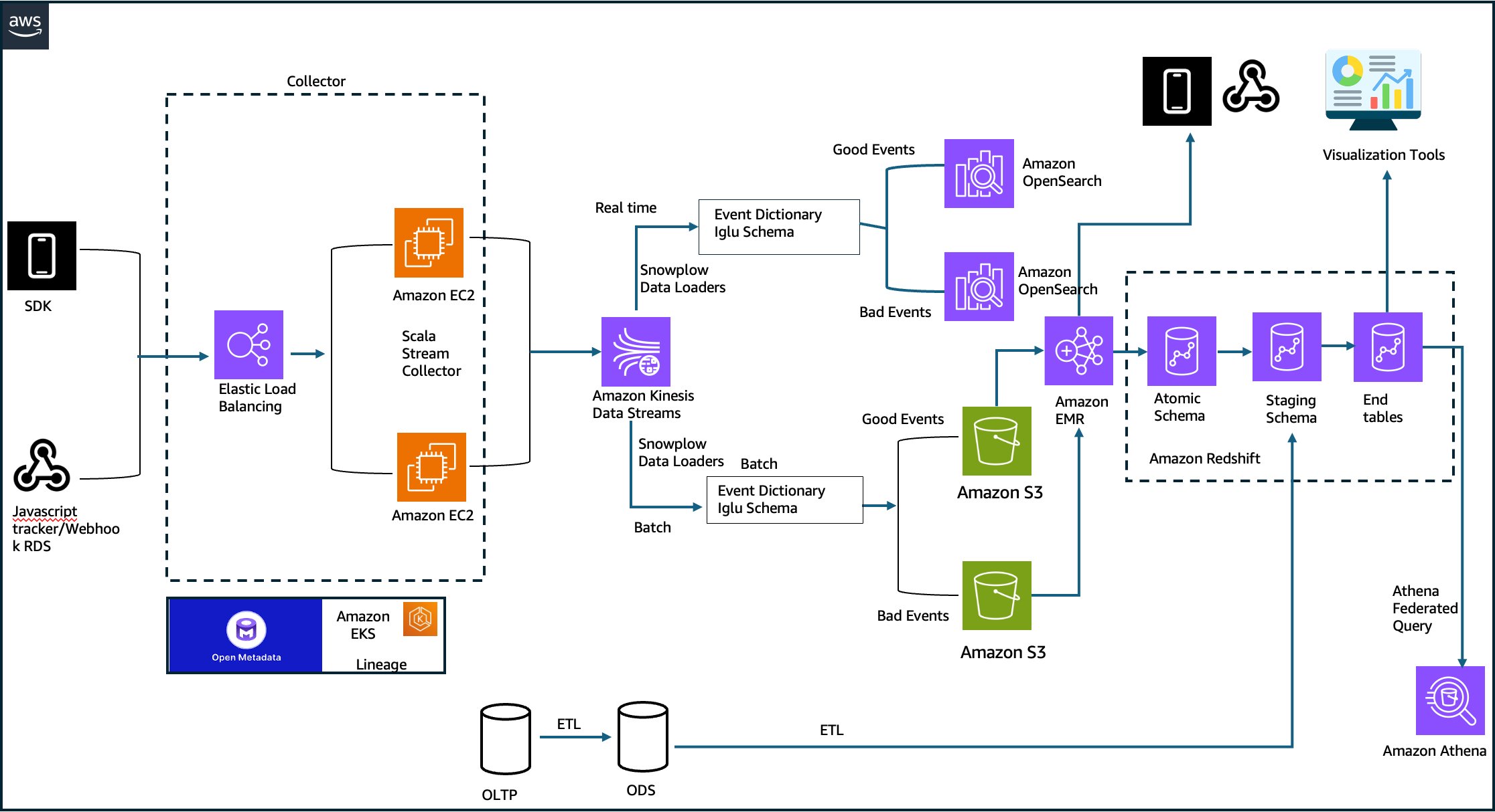
BigBasket implemented a sophisticated dual-path architecture for processing clickstream data from mobile apps and web interactions:

  • Real-time path: Data flows through Scala stream collectors on Amazon Elastic Compute Cloud (Amazon EC2) (behind Elastic Load Balancing) to Amazon Kinesis Data Streams and Amazon OpenSearch Service for immediate insights into customer behavior. This path is necessary when you need to react to user actions within seconds, for example detecting fraud or personalizing experiences in real time.
  • Batch path: The batch path validates data, stores it in Amazon S3, processes it through Amazon EMR, and loads it into Amazon Redshift for comprehensive historical analysis. This path handles data quality checks, enrichment, and aggregation for long-term analytics.

The trade-off between these approaches is latency versus completeness. Real-time processing gives you speed but may sacrifice some data quality checks, while batch processing provides accuracy but introduces delay. This dual approach achieves both immediate operational insights and deep analytical capabilities, letting you optimize for different use cases.

The following diagram shows how the clickstream data is handled and effectively processed today.

BigBasket’s dual-path clickstream processing architecture with real-time and batch paths on AWS

The results: measurable business impact

The data platform transformation achieved significant results across multiple dimensions:

Technical improvements

  • Near real-time data: Achieved near real-time data availability for dashboards within 3–5 minutes, replacing previously day-old data.
  • Rapid failure recovery: Pipeline failure re-runs now complete in minutes instead of hours.
  • Comprehensive governance: Full control over data governance with robust observability, lineage, data accuracy, and consistency.
  • Enhanced scalability: Successfully handling over 35,000 reports and dashboards with over 1,000 dataset refreshes.

Business outcomes

  • On-time delivery: Improved monitoring with real-time insights on low-performing stores.
  • Stock availability: Reduced operational issues with visibility into key bottlenecks.
  • Stock forecasting: Improved accuracy and availability of top-selling SKUs.
  • Dark store productivity: Enhanced productivity of warehouse executives across all operations.

Key takeaways: lessons for modern data platforms

BigBasket’s journey offers valuable insights for organizations facing similar challenges:

  1. Quick commerce needs quick observability. In the fast-paced world of quick commerce, faster decision-making directly improves business metrics. Real-time data isn’t a luxury. It’s a necessity.
  2. Embrace ELT for real-time needs. Shifting from traditional ETL to an extract, load, transform (ELT) pattern within a lakehouse architecture is important to unlock near real-time analytics capabilities.
  3. A lakehouse delivers speed and governance. Modern lakehouse architectures don’t force trade-offs. You can achieve both fast data availability and comprehensive control, lineage, and accuracy.
  4. Focus on operational resilience. Designing for rapid failure recovery (re-runs in minutes, not hours) is necessary for maintaining data availability and business trust, especially in customer-facing operations.
  5. Incremental migration. You don’t need to rebuild everything. Evolve your current Amazon S3 data lake or reuse your existing investments in Amazon Redshift to build the data lakehouse capabilities.

The road ahead

BigBasket continues to innovate, now moving to adopt Amazon SageMaker Unified Studio to access all lakehouse components in a simplified manner across the enterprise. This next evolution will further streamline data access and accelerate insights across teams.

The company’s transformation demonstrates that with the right architecture and AWS services, organizations can turn data infrastructure challenges into competitive advantages, delivering not only better analytics but better customer experiences.

As you plan your own lakehouse implementation, use these patterns and lessons learned to accelerate your journey and avoid common pitfalls.


About the authors

Naga Sandeep Grandhi

Naga Sandeep Grandhi

Sandeep is an engineering leader at BigBasket, driving data platform and cloud architecture initiatives, including the next-gen data lake built for scale, reliability, and real-time insights.

Vikram Kumar

Vikram Kumar

Vikram is a Principal Engineer at BigBasket, where he leads the data engineering team. He specializes in designing and scaling modern data platforms on AWS, enabling BigBasket to process large-scale data efficiently and power data-driven decision-making across the organization.

Annie Mattoo

Annie Mattoo

Annie is a Sr. Analytics Specialist at AWS, bringing over 15+ years of expertise in helping customers with their DATA & AI journeys. She has successfully led customer teams to seamlessly adopt AWS Data & AI services and has worked with Fortune 500 customers across the globe in her previous roles.

Vineet Thapliyal

Vineet Thapliyal

Vineet is an Enterprise Account Manager at Amazon Web Services (AWS) in Bengaluru, India, where he manages strategic cloud and generative AI engagements across some of India’s largest conglomerates spanning energy, retail, and technology. He is passionate about helping enterprises unlock business value through AI/ML, cloud modernization, and industry-specific innovation — from renewable energy analytics to retail transformation at scale.

Anirudh Chawla

Anirudh Chawla

Anirudh is an Analytics Solution Architect at AWS. He helps organization empowers businesses to harness their data effectively through AWS’s analytics platform. His interest lies in building highly available distributed systems.

AWS Weekly Roundup: Claude Sonnet 5 on AWS, Amazon WorkSpaces for AI agents, AWS service availability updates, and more (July 6, 2026)

Post Syndicated from Daniel Abib original https://aws.amazon.com/blogs/aws/aws-weekly-roundup-claude-sonnet-5-on-aws-amazon-workspaces-for-ai-agents-aws-service-availability-updates-and-more-july-6-2026/

A couple of editions ago I wrote about what I find so energizing about working with startups. Last week I got a fresh dose of it: I spent a few days with the AWS Startups team, listening to stories of founders talking about the problems they’re actually solving. One story that stayed with me came from Marco Negreiros, founder of EyeCare Health, a Brazilian healthtech expanding access to eye care. He shared a striking fact: more than 70% of Brazilian municipalities don’t have a single ophthalmologist. His answer was to put a vision test on the one device almost everyone already carries, the smartphone, so a basic eye screening no longer depends on living near a clinic. Watching a founder turn a gap that big into something that concrete is exactly why I love this space.

AWS Startups team get-together with founders in Brazil

This week, I’ll take a closer look at some key launches, and then cover the quarterly AWS Service Availability updates.

Last week’s launches
Here are some of the launches covered from this past week in the AWS News Blog:

Here are some launches and updates that caught my attention:

For a full list of AWS announcements, be sure to keep an eye on the What’s New with AWS page.

AWS Service Availability Updates
When the availability of an AWS service or feature changes, we provide customers guidance in AWS Product Lifecycle Changes on available alternatives and support for migration so that disruptions to your operations are minimized. The following lifecycle changes were updated on June 30, 2026.

Services moving to Maintenance (no longer accessible to new customers starting July 30, 2026):

Services entering Sunset:

Services reaching End of Support (as of June 30, 2026):

  • Amazon Chime SDK – Carrier Voice Focus
  • Amazon SageMaker AI – Ground Truth Plus

We understand that changes in availability can impact your operations. For specific guidance, consult the relevant service documentation or contact AWS Support.

Upcoming AWS events
Check your calendar and sign up for upcoming AWS events:

  • AWS Summits – AWS Summits are free events that bring the cloud and AI community together to connect, learn, and explore the latest technologies. Browse the full calendar to find a Summit near you in the second half of 2026.
  • AWS Community Days – Community-led conferences where content is planned, sourced, and delivered by community leaders. If you’re in Latin America, don’t miss AWS Community Day Belo Horizonte on August 22. Registration is open at awscommunityday.com.br.

Join the AWS Builder Center to connect with builders, share solutions, and access content that supports your development. Browse here for upcoming AWS-led in-person and virtual events and developer-focused events.

That’s all for this week. Check back next Monday for another Weekly Roundup!

– Daniel Abib

This post is part of our Weekly Roundup series. Check back each week for a quick roundup of interesting news and announcements from AWS!

Deploy modern data platforms in minutes with MDAA

Post Syndicated from Sudeshna Dash original https://aws.amazon.com/blogs/big-data/deploy-modern-data-platforms-in-minutes-with-mdaa/

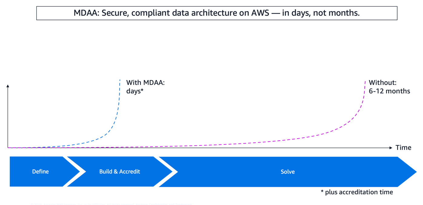
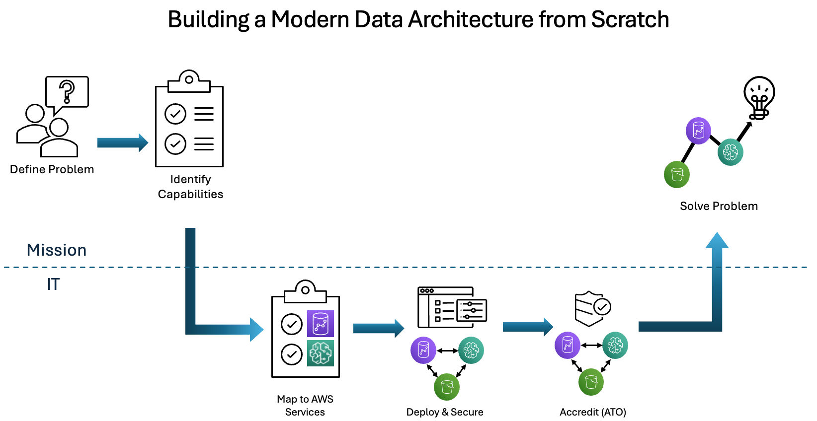
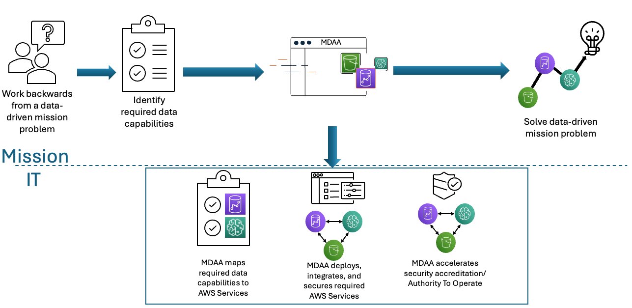
Modern Data Architecture Accelerator (MDAA) is an open source framework that replaces infrastructure code with concise YAML configuration, so your team can deploy a governed, production-ready data architecture, reducing deployment time from months to weeks (depending on complexity and team experience).

Organizations building modern data architecture on AWS face a critical challenge: deploying production-ready, governed infrastructure traditionally requires 6–12 months of custom development, thousands of lines of infrastructure code, and continuous remediation cycles to maintain security and compliance. Governance is often added incrementally, treated as an afterthought that creates compliance gaps and engineering rework.

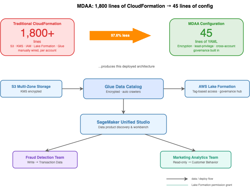
MDAA addresses this by replacing infrastructure code with concise YAML configuration, achieving up to 97.6 percent code reduction (from approximately 1,800 lines of AWS CloudFormation to 45 lines of MDAA YAML) while embedding governance from the start. The complete Governed Lakehouse Starter Kit deploys 491 AWS resources across 12 stacks from approximately 450 lines of YAML configuration, representing a 66x verbosity ratio where each line automatically expands into production-ready infrastructure.

In this post, we explore how MDAA transforms data architecture development from months of manual coding to production-ready deployment through configuration-driven infrastructure and embedded governance, examine a real customer transformation, and provide a clear implementation pathway for your own data modernization journey.

Customer use case and challenge

A university system office needed to modernize its analytics architecture across 17 campuses while managing sensitive educational data. Their third-party dependency created bottlenecks that slowed feature implementation from weeks to months, and their IT team lacked the cloud skillsets to build modern infrastructure independently.

With MDAA, they achieved:

  • 95 percent reduction in time-to-value for dashboard and feature implementation (from weeks to hours).
  • 17 campuses integrated into a unified, secure architecture.
  • 7.2TB of data and over 8,000 dashboards migrated successfully.
  • Significant cost savings by removing third-party dependencies and reducing license costs.
  • Enhanced security posture for external stakeholders accessing sensitive educational data.

The team used MDAA to implement a modernization strategy with continuous integration and continuous delivery (CI/CD) for automated deployment. The architecture now supports rapid response to stakeholder requests while maintaining strict data governance through AWS Lake Formation.

Their transformation demonstrates what becomes possible when governance is embedded from launch rather than added incrementally, moving from months-long manual development to weeks of production-ready deployment through configuration-driven infrastructure.

Solution: MDAA and its value propositions

MDAA’s capabilities stem from its modular, composable architecture. The accelerator provides over 40 pre-built modules that encapsulate AWS best practices for security, governance, and operational excellence. Organizations describe the outcomes they want in MDAA-specific YAML configuration files (not CloudFormation or Terraform YAML) and the accelerator automatically translates these configurations into AWS Cloud Development Kit (AWS CDK) constructs, which then deploy via CloudFormation with embedded governance.

Configuration over code. The MDAA framework takes a fundamentally different approach: describe the outcomes you want in YAML, and the accelerator deploys production-ready infrastructure with embedded governance. Consider deploying a governed data lake where fraud detection teams need write access to transaction data, while marketing analytics teams require read-only access to customer behavior data. Traditional approaches require over 1,800 lines of CloudFormation across Amazon Simple Storage Service (Amazon S3) buckets, AWS Key Management Service (AWS KMS) keys, AWS Identity and Access Management (IAM) policies, and Lake Formation permissions. With MDAA, the same governed data lake is expressed in 45 lines of configuration, a 97.6 percent reduction, while helping you apply encryption, least-privilege access, and cross-account governance as built-in defaults.

The configuration deploys multi-zone S3 storage with KMS encryption, Lake Formation permissions with tag-based access control (TBAC) enabled, Amazon SageMaker Unified Studio for data product discovery, and encrypted AWS Glue Data Catalog with automated crawlers. All permissions flow through Lake Formation rather than individual IAM policies.

Embedded governance from day one. Governance is declared in YAML and deployed alongside infrastructure from the first run. Fine-grained access controls, encrypted data catalogs, data quality validation, audit trails, and sensitive data classification are all part of the same configuration. MDAA’s Governed Lakehouse starter kit defines an entire governed data architecture in roughly 450 lines of YAML, which produces approximately 29,700 lines of CloudFormation across 12 stacks (a 98.5 percent reduction in infrastructure code).

Modular, composable architecture. Each module is purpose-built to handle a specific capability within the data architecture. Modules communicate through AWS Systems Manager Parameter Store, passing resource identifiers (Amazon Resource Names (ARNs), IDs, and names) between stacks. This approach removes hardcoded dependencies. A KMS key created in one module can be referenced by another through parameter resolution, with all dependencies resolved automatically at deployment time.

The diagram illustrates the deployed architecture and team-level access flow that MDAA generates from the 45-line configuration.

Progressive architecture patterns. MDAA provides four reference architecture patterns that align to progressive stages of data infrastructure maturity:

  • Basic Data Lake deploys a governed data lake with built-in security controls, data quality checks, centralized metadata management using AWS Lake Formation and AWS Glue.
  • Data Science Platform extends the data lake with Amazon SageMaker notebooks, feature stores, and machine learning (ML) pipelines so data science teams can experiment and train models on governed data.
  • SageMaker Unified Studio adds a single interface for analytics and ML collaboration, connecting data engineers, analysts, and data scientists in one workspace.
  • Generative AI Platform layers Amazon Bedrock and Retrieval Augmented Generation (RAG) capabilities on top of your existing data foundation, so teams can build generative AI applications grounded in enterprise data.

Each pattern builds the one before it. You can start with the Basic Data Lake and adopt additional patterns as your team’s needs grow. MDAA’s modular design means you add capabilities without rearchitecting what you already deployed.

The infrastructure is versioned through GitHub, repeatable across environments, and auditable through comprehensive AWS CloudTrail logging. Data engineers focus on data pipelines and business logic while MDAA manages infrastructure complexity and governance integration. This represents the fundamental shift: from writing infrastructure code to describing the outcomes you want through configuration, with governance embedded from the start.

Use case of MDAA: Governed data architecture

DataOps teams spend significant time on governance tasks, including permissions management, compliance validation, and access control, rather than building pipelines and analytics. These aren’t data problems, they’re governance problems that consume engineering capacity meant for higher-value work. MDAA addresses this at the architectural level. Governance is declared in YAML and deployed alongside infrastructure from the first run.

The following sections walk through how each governance module works in practice.

Publish, discover, subscribe, and consume data products between business units: SageMaker Unified Studio

Amazon SageMaker Unified Studio provides a governed data catalog where data producers publish data products, and consumers discover and subscribe to them. Your deployment with MDAA includes a pre-configured domain, blueprints (managed and custom), projects, and environment profiles, all defined in a single configuration file:

# sagemaker.yaml --- 16 lines that deploy 114 CloudFormation resources
domains:
  domain1:
    dataAdminRole:
      id: ssm:/{{org}}/govern1/generated-role/data-admin/id
    description: SMUS Domain 1
    userAssignment: MANUAL

    tooling:
      vpcId: '{{context:vpc_id}}'
      subnetIds:
        - '{{context:private_subnet_id1}}'
        - '{{context:private_subnet_id2}}'

    groups:
      team1:
        ssoId: '{{context:team1-group-sso-id}}'
      team2:
        ssoId: '{{context:team2-group-sso-id}}'

Behind this configuration, MDAA deploys an Amazon SageMaker Unified Studio domain with dedicated KMS keys, execution and provisioning roles, and single sign-on group profiles for team access. Data producers tag and publish assets with metadata, ownership, and classification. Consumers browse a searchable catalog, see only authorized assets, and request access through a governed workflow. Cross-account and cross-business-unit data sharing flows through a subscription model, ensuring every access grant is tracked, auditable, and revocable.

Use case of MDAA: Restricting access to cardholder data using Lake Formation

AWS Lake Formation provides fine-grained access control at database and table levels, removing manual IAM policy management. MDAA deploys AWS Lake Formation with pre-configured settings that disable IAMAllowedPrincipals, the critical governance setting that ensures all permissions flow through centralized governance:

# lakeformation-settings.yaml --- 6 lines that deploy 25 CloudFormation resources
lakeFormationAdminRoles:
  - id: generated-role-id:data-admin
createCdkLFAdmin: true
createDataZoneAdminRole: true
iamAllowedPrincipalsDefault: false

That last flag is the single most important governance setting in the platform. Without it, an IAM principal with glue:GetTable can read tables in the catalog, bypassing the entire access control model. Most manual setups miss this or defer it.

With the data lake configuration, you declare roles and access policies in YAML where admins get full control, engineers get read access to curated data, extract, transform, and load (ETL) roles get scoped write access, and MDAA compiles them into the correct S3 bucket policies and Lake Formation registrations.

Use case of MDAA: Ensuring data integrity with AWS Glue Data Quality

AWS Glue Data Quality runs automated validation rulesets continuously as part of the pipeline, not as periodic batch checks. MDAA’s data quality module supports over 15 built-in rule types, from completeness and uniqueness checks to statistical thresholds and data freshness validation:

# data-quality.yaml
projectName: example-project

rulesets:
  customer-data-quality:
    description: Validate customer data completeness and uniqueness
    targetTable:
      databaseName: project:databaseName/customer-data
      tableName: customers
    ruleset:
      - ruleType: IsComplete
        column: customer_id
      - ruleType: Uniqueness
        column: email
        comparisonOperator: ">"
        threshold: 0.95
      - ruleType: RowCount
        comparisonOperator: ">"
        value: 100

Quality metrics flow into Amazon CloudWatch for real-time alerting. If anomalies are detected, automated workflows quarantine affected records and alert data engineering teams before issues reach downstream consumers.

Protecting metadata at rest: AWS Glue Data Catalog encryption

Table schemas, column names, and partition structures can reveal sensitive information about an organization’s data architecture, even without access to the underlying data. AWS Glue Catalog Encryption secures metadata at rest using AWS KMS-managed keys. MDAA configures catalog encryption by default, so schema definitions and connection passwords are encrypted from initial deployment without requiring manual key management setup. Access to catalog metadata follows the same Lake Formation governance controls applied to the data itself, so teams see only the schemas that they’re authorized to query.

Auditing every data access event: CloudTrail integration

Every data access event must be logged and attributable to a specific identity. Without a complete audit trail, demonstrating compliance during a regulatory review becomes a manual, error-prone process. AWS CloudTrail captures API-level activity across the data infrastructure, recording who accesses what data, when, and from which service. MDAA configures CloudTrail integration by default, so audit logging is active from initial deployment rather than added retroactively. Log data flows into a centralized, tamper-resistant store, giving compliance teams a single location to query access history across all business units and accounts.

Identifying sensitive data automatically: Macie integration

In large environments, sensitive information spreads across dozens of S3 buckets through pipelines, transforms, and ad hoc data drops, and self-reporting data owners consistently produce gaps. Amazon Macie uses machine learning to automatically discover and classify sensitive data in S3, surfacing findings at the object level without manual tagging. MDAA configures Macie across your S3 buckets during deployment, routing findings to Amazon EventBridge where automated workflows can alert owners or trigger remediation.

Together, these controls form a layered defense: Lake Formation governs access to cataloged data, Glue Data Quality validates integrity on arrival, and Macie identifies sensitive data that lands outside governed pipelines to reduce compliance risk.

Multi-account data mesh

MDAA provides extensive support for multi-account data mesh setups, with decentralized data ownership across business units and centralized governance. The data mesh starter kit supports cross-account data product publishing and consumption, allowing organizations to scale data sharing while maintaining consistent security and compliance controls.

Technical implementation

Ready to deploy your modern data architecture? Here are the resources to get started:

MDAA Implementation Guide provides detailed instructions for deploying all starter packages, including architecture patterns, configuration examples, security best practices, and troubleshooting guidance.

MDAA Hands-on Workshop offers step-by-step guided implementation with AWS experts. The workshop covers configuration management best practices, implementation patterns, hands-on labs with real-world scenarios, and cleanup instructions.

GitHub Repository and Documentation provide source code, module reference, and comprehensive documentation.

Organizations approach MDAA from different starting points. Some modernize existing data architectures, migrating from on-premises infrastructure or legacy cloud architectures. Others build new architectures for artificial intelligence and machine learning (AI/ML) initiatives or generative AI applications. Financial services organizations require PCI-DSS compliance from day one. Healthcare organizations need controls that can help support HIPAA. Each journey benefits from MDAA’s configuration-driven approach and embedded governance.

Conclusion

MDAA transforms data architecture development from months of manual coding to production-ready deployment. Configuration-driven infrastructure reduces development time by 40–60 percent while embedding governance from the start. The university system’s 95 percent reduction in time-to-value demonstrates the outcome: organizations deploy secure, compliant, governed data architectures in weeks rather than months.

Financial services organizations can deploy architectures to help them align with PCI-DSS compliance requirements using Lake Formation access controls, Glue Data Quality validation, SageMaker Unified Studio data discovery, comprehensive CloudTrail audit trails, and automated Macie data classification, all inherited from configuration rather than built manually.

Data architecture journeys need not follow six-month timelines with governance added incrementally. MDAA provides an alternative: describe the outcomes you want through YAML configuration, inherit pre-validated security controls, and deploy production-ready infrastructure with comprehensive governance from initial deployment.

Security and compliance is a shared responsibility between AWS and the customer. For more information, see the AWS Shared Responsibility Model.

Need help or have questions? Contact AWS ProServe for personalized guidance on selecting the right package and deployment strategy for your organization.


About the author

Sudeshna Dash

Sudeshna Dash

Sudeshna is a Data Scientist at AWS Professional Services based in Berlin, Germany. She specializes in data architecture, generative AI, and agentic AI systems on AWS. Sudeshna is a contributor to the Modern Data Architecture Accelerator (MDAA) open-source project and helps customers design and deploy governed, production-ready data and AI/ML architectures on AWS.

John Reynolds

John Reynolds is a Principal Engineer with AWS Professional Services based in Seattle, Washington. He leads the architecture and development of Modern Data Architecture Accelerator (MDAA), focusing on turning proven delivery patterns into reusable, production-ready foundations that customers can adopt and extend at scale.

Getting your SMS short code production-ready with AWS End User Messaging

Post Syndicated from Harshvardhan Chunawala original https://aws.amazon.com/blogs/messaging-and-targeting/getting-your-sms-short-code-production-ready-with-aws-end-user-messaging/

Getting your Short Message Service (SMS) short code production-ready requires you to configure the Amazon Web Services (AWS) infrastructure that controls how your messages are sent, monitored, and protected. You have provisioned your short code, and it is active on carrier networks. In this post, we walk through that setup using AWS End User Messaging SMS, covering 12 configuration steps from compliance through phased traffic migration. Total estimated time is 2 to 4 hours of configuration plus 1 to 3 business days for limit increase approvals.mess

The guide to SMS short codes with AWS End User Messaging covers the application and registration process up through provisioning. This post picks up from that point and provides an operational readiness walkthrough that takes you from “Active” status to confidently sending your first production message, including a final validation step to confirm readiness.

The following diagram shows the end-to-end message flow and event routing architecture covered in this walkthrough.

End-to-end SMS short code architecture showing message flow from sender through AWS End User Messaging SMS to carriers and recipient handsets, with event routing to Amazon CloudWatch, Amazon Simple Notification Service (Amazon SNS), and Amazon Data Firehose destinations

Prerequisites

You need the following to follow along with this walkthrough:

  1. An AWS account with access to the AWS End User Messaging SMS console.
  2. A short code with Active status in the AWS Management Console (carrier provisioning finished).
  3. Permissions to create AWS Identity and Access Management (IAM) roles, Amazon CloudWatch Log Groups, and Amazon Simple Notification Service (Amazon SNS) topics.
  4. AWS Command Line Interface (AWS CLI) v2 or an AWS SDK installed and configured.
  5. Your approved registration documentation, including the service name, keyword responses, and message templates submitted to carriers.

Step 1: Verify your short code is active and delivering

Navigate to the AWS End User Messaging SMS console, choose Phone numbers, and locate your provisioned short code. Confirm that the status shows Active, then send a test message to a phone number you control using the SendTextMessage API or the console test feature. Verify delivery on your handset.

Carrier-side activation can take up to 24 to 48 hours to fully propagate across all networks after provisioning finishes. If the console shows Active but your test message does not arrive, submit a support case so the team can verify propagation status with the carrier.

You can also verify using the AWS CLI:

aws pinpoint-sms-voice-v2 send-text-message \
    --destination-phone-number "+15555550100" \
    --origination-identity "12345" \
    --message-body "Test message from short code" \
    --message-type TRANSACTIONAL \
    --configuration-set-name "prod-otp-shortcode"
# Replace +15555550100 with your test phone number, 12345 with your short
# code, and prod-otp-shortcode with your configuration set name from Step 3.

Step 2: Configure keywords and verify message compliance

US carriers require every short code to respond to HELP and STOP keywords. You defined these during your registration, and this step confirms they are configured correctly in your account.

In the SMS console, choose Phone numbers, select your short code, and choose the Keywords tab. Verify that STOP returns the opt-out response you submitted during registration, and that HELP returns your support contact response (which must include a phone number or email). Add any custom keywords your use case requires, such as YES for double opt-in confirmation flows. You can manage keywords programmatically using the PutKeyword API.

To add or update a keyword programmatically:

aws pinpoint-sms-voice-v2 put-keyword \
    --origination-identity "12345" \
    --keyword "YES" \
    --keyword-message "You have confirmed your subscription to Acme Health Alerts. Msg&data rates may apply. Reply STOP to opt out." \
    --keyword-action AUTOMATIC_RESPONSE
# Replace 12345 with your short code, YES with your custom keyword, and the
# keyword-message text with your approved response.

To verify your current keyword configuration:

aws pinpoint-sms-voice-v2 describe-keywords \
    --origination-identity "12345"
# Replace 12345 with your short code.

Beyond keyword configuration, carrier compliance does not end at registration approval. The content you send in production must stay aligned with what carriers reviewed and approved. Here is what to keep consistent.

Use the exact brand or program name from your approved registration across all keyword responses, confirmation messages, and outbound templates. If carriers approved your registration under “Acme Health Alerts,” every message your short code sends should reference that name. Mixing variations creates inconsistencies that auditors flag during reviews. For example, do not use the company name in one message and the product name in another.

Your HELP, STOP, and confirmation responses must match the templates submitted during registration. Do not add or remove opt-out language, change frequency disclosures, or alter customer care contact details post-approval without updating the registration through a support case. If your organization operates multiple domains, use the domain documented in the registration. For example, you might have one domain for the application and another for marketing. Carrier reviewers cross-reference message content, opt-in screenshots, and privacy policy URLs with what was submitted.

Humans conduct carrier reviews, and message content that is concise and limited to the essentials is reviewed consistently. All messages must remain under 160 characters.

Step 3: Create a configuration set with event destinations

A configuration set controls where your SMS delivery events are streamed and which event types are captured. Without one, you are limited to the basic events that AWS End User Messaging SMS sends to Amazon EventBridge by default. These default events omit recipient details and full carrier response context.

Create a configuration set with a descriptive name such as prod-otp-shortcode or marketing-sc-us. Then create at least one event destination. The three main options are Amazon CloudWatch Logs (for operational monitoring and alarming), Amazon SNS (for real-time event fanout to downstream systems), and Amazon Data Firehose (for durable archival and analytics).

Amazon Data Firehose typically delivers to an Amazon Simple Storage Service (Amazon S3) bucket, where you can query delivery history using Amazon Athena for compliance audits or delivery pattern analysis.

# Create the configuration set
aws pinpoint-sms-voice-v2 create-configuration-set \
    --configuration-set-name "prod-otp-shortcode"

# Add a CloudWatch Logs event destination
aws pinpoint-sms-voice-v2 create-event-destination \
    --configuration-set-name "prod-otp-shortcode" \
    --event-destination-name "otp-delivery-logs" \
    --matching-event-types TEXT_DELIVERED TEXT_FAILED TEXT_QUEUED TEXT_CARRIER_UNREACHABLE TEXT_TTL_EXPIRED \
    --cloud-watch-logs-destination '{
        "IamRoleArn": "arn:aws:iam::123456789012:role/SMSEventsToCloudWatch",
        "LogGroupArn": "arn:aws:logs:us-east-1:123456789012:log-group:/aws/sms/prod-otp-shortcode"
    }'
# Replace prod-otp-shortcode with your configuration set name, otp-delivery-logs
# with a descriptive destination name, and the ARN values with your IAM role ARN
# (must have logs:PutLogEvents permission) and CloudWatch Log Group ARN.

Important: When sending messages with SendTextMessage, always specify your ConfigurationSetName parameter so events route to the appropriate destination.

Required event types

Event type Description
TEXT_DELIVERED Message successfully delivered to recipient handset.
TEXT_FAILED Message delivery failed.
TEXT_QUEUED Message accepted and queued for delivery.
TEXT_CARRIER_UNREACHABLE Carrier network unreachable.
TEXT_TTL_EXPIRED Message expired before delivery.

For a detailed walkthrough of configuration sets including multi-tenant architectures, see How to send SMS using configuration sets with AWS End User Messaging.

Step 4: Create a phone pool and associate your short code

A pool is a logical container that groups origination identities and controls routing behavior. Creating one gives you deterministic control over which number sends your messages and how opt-outs are enforced.

# Create the pool
aws pinpoint-sms-voice-v2 create-pool \
    --origination-identity "12345" \
    --iso-country-code "US" \
    --message-type TRANSACTIONAL

# Disable shared routes so only your short code is used
aws pinpoint-sms-voice-v2 update-pool \
    --pool-id "pool-1234567890abcdef0" \
    --shared-routes-enabled false
# Replace 12345 with your short code, US with your destination country code,
# and pool-1234567890abcdef0 with the Pool ID returned by create-pool.

Configuration parameters

Parameter Recommended value Rationale
Pool name us-otp-pool Descriptive, environment-prefixed.
SharedRoutesEnabled False Prevents fallback to shared routes; only your short code is used.
Opt-out list Associate one Manages opt-out state per use case.
IsoCountryCode US Restricts to destination country your short code serves.

If you operate multiple use cases on separate short codes, create a dedicated pool for each. For example, use one short code for one-time password (OTP) traffic and another for transactional notifications. This isolation means a recipient opting out of marketing messages does not lose access to authentication codes.

Step 5: Request your throughput increase

Short codes start at a default of 100 messages per second (MPS). If your production volume will exceed this, request an increase before your launch date rather than after traffic is flowing.

Create a case in the AWS Support Center, choose Service limit increase, then choose End User Messaging SMS. Provide your short code phone number, requested MPS, use case description, and expected peak volume. Allow 1 to 3 business days for processing.

To estimate your required MPS:

Required MPS = (Peak hourly volume / 3,600) x 2

Short codes support scaling to thousands of MPS, so start with a value that covers your expected peak and request further increases as traffic grows.

Step 6: Request a spending limit increase

AWS accounts have a default monthly SMS spending limit. To keep delivery uninterrupted at your expected volume, request an increase that accommodates your projected monthly spend before you begin sending.

Create a support case under Service limit increase > End User Messaging SMS > Account Spend Threshold. Provide your estimated monthly spend, use case description, and website URL.

For details, see Requesting increases to your monthly SMS spending quota.

Step 7: Restrict destination countries

If your short code serves a single country (US-only, for example), restrict sending to that country. This protects your account from artificially inflated traffic (SMS pumping). In pumping attacks, messages are routed to international premium-rate numbers, generating significant charges.

In the SMS console, navigate to Account settings, then choose Countries and keep only the countries you intend to send to. The pool-level IsoCountryCode restriction from Step 4 provides an additional enforcement layer at the sending path. Combining account-level country restrictions with pool-level country codes gives you two independent controls that both must be satisfied before a message is sent internationally.

For a detailed walkthrough on SMS fraud prevention controls, see Defending against SMS pumping: new AWS features to help combat artificially inflated traffic.

Step 8: Set up monitoring and alarms

With event destinations configured in Step 3, build proactive alerting that surfaces delivery trends before they affect your end users.

Alarm Metric / Source Threshold
Delivery success rate CloudWatch SMS metrics Alert when below 95%.
Spend threshold CloudWatch billing metric Alert at 80% of monthly limit.
Delivery failures Amazon EventBridge rule on TEXT_FAILED Route to Amazon SNS topic or AWS Lambda.
Carrier unreachable Amazon EventBridge rule on TEXT_CARRIER_UNREACHABLE Route to Amazon SNS topic or AWS Lambda.

Build a CloudWatch dashboard showing messages sent per minute, success versus failure breakdown, and spend accumulation over time.

You can also configure Amazon EventBridge to notify you of registration status changes. AWS End User Messaging SMS publishes events for statuses including REQUIRES_UPDATES, REVIEWING, and PROVISIONING, which is useful if a carrier requests changes during a proactive audit after your short code is already active.

For metric details, see Monitoring SMS activity with Amazon CloudWatch.

Step 9: Track OTP verification success (if applicable)

If your short code delivers OTP or two-factor authentication (2FA) codes, track end-to-end verification success in addition to carrier delivery receipts. A “delivered” status at the carrier level does not confirm the end user received and entered the code.

Tracking verification rates gives you insight into latency patterns when codes expire before arrival, geographic delivery trends, and opportunities to improve conversion. Some use cases involve asynchronous processing where several minutes of computation occur before the SMS is sent. For these, measure the full round-trip from the triggering action to message delivery. This separates application-side latency from carrier-side delivery latency.

For implementation guidance, see Track OTP success with AWS End User Messaging SMS feedback.

Step 10: Set up cost visibility

SMS costs include AWS charges plus per-message carrier surcharges. Setting up cost visibility from day one lets you track spend trends, catch anomalies early, and optimize over time.

Start by activating AWS Cost Explorer and creating a cost allocation tag for your SMS workload. Then configure an AWS Budget with threshold alerts. For example, you might notify at 80% of projected monthly spend. This gives you advance warning of unexpected cost increases, whether from traffic spikes, retry loops, or blocked-country leakage.

Step 11: Plan your traffic migration

A phased rollout validates delivery performance at each stage before you increase volume.

Start with a canary phase (Day 1 to 3) where you route 5 to 10% of traffic to the short code and monitor delivery rates, latency, and event logs. Move to a ramp phase (Day 3 to 7) at 50%, validating throughput and carrier-level delivery across your recipient base. Finish the full migration (Day 7+) at 100%. Decommission your previous origination identity only after confirming stability for at least 48 hours.

Step 12: Validate production readiness and send

Before declaring your short code production-ready, run through the following validation checks:

  1. Confirm your CloudWatch dashboard shows events flowing for TEXT_DELIVERED and TEXT_FAILED (from Step 3).
  2. Send a test message that triggers your STOP keyword. Verify the correct opt-out response is returned and the phone number appears in your opt-out list.
  3. Send a test message that triggers your HELP keyword. Verify the response matches your approved registration.
  4. Check your MPS quota in the support case response (from Step 5). Confirm it matches or exceeds your calculated peak.
  5. Review your country restrictions (from Step 7). Attempt to send a message to a blocked country and confirm it is rejected.
  6. Verify your CloudWatch alarm fires by temporarily lowering the threshold, or by checking that the alarm state is not INSUFFICIENT_DATA.

After all six checks pass, you are ready to begin your phased migration (Step 11) and scale to full production traffic. At this point, your short code is configured, monitored, compliant, and protected.

Automate with a validation script

You can use an AI coding assistant such as Kiro to generate a validation script tailored to your environment. Try a prompt like: “Write a boto3 script that validates my SMS short code is production-ready by checking Active status, HELP/STOP keywords, configuration set existence, and pool association using the pinpoint-sms-voice-v2 client.”

Refine the prompt with specifics from the following reference implementation, such as exact API names, filter parameters, and output format, to match your requirements.

The following script is an example of what that output looks like:

import boto3
import sys

SHORT_CODE = "12345"  # TODO: Replace with your short code (e.g., "67890")
POOL_ID = "pool-1234567890abcdef0"  # TODO: Replace with your pool ID from Step 4
CONFIG_SET_NAME = "prod-otp-shortcode"  # TODO: Replace with your configuration set name from Step 3

client = boto3.client("pinpoint-sms-voice-v2")

# Note: For accounts with many resources, implement NextToken pagination
# on describe_* calls. This script assumes results fit in a single page.


def check_short_code_active():
    """Step 1: Verify short code is Active."""
    response = client.describe_phone_numbers(
        Filters=[
            {"Name": "status", "Values": ["ACTIVE"]},
            {"Name": "number-type", "Values": ["SHORT_CODE"]}
        ]
    )
    numbers = [
        n for n in response["PhoneNumbers"]
        if n["PhoneNumber"] == SHORT_CODE
    ]
    assert len(numbers) > 0, f"Short code {SHORT_CODE} not found or not Active"
    print(f"[PASS] Short code {SHORT_CODE} is Active")


def check_keywords_configured():
    """Step 2: Verify HELP and STOP keywords exist."""
    response = client.describe_keywords(OriginationIdentity=SHORT_CODE)
    keyword_names = [kw["Keyword"].upper() for kw in response["Keywords"]]
    assert "STOP" in keyword_names, "STOP keyword not configured"
    assert "HELP" in keyword_names, "HELP keyword not configured"
    print("[PASS] HELP and STOP keywords configured")


def check_configuration_set():
    """Step 3: Verify configuration set exists."""
    response = client.describe_configuration_sets(
        ConfigurationSetNames=[CONFIG_SET_NAME]
    )
    assert len(response["ConfigurationSets"]) > 0, f"Configuration set {CONFIG_SET_NAME} not found"
    print(f"[PASS] Configuration set '{CONFIG_SET_NAME}' exists")


def check_pool_association():
    """Step 4: Verify pool exists and short code is associated to it."""
    response = client.describe_pools(PoolIds=[POOL_ID])
    assert len(response["Pools"]) > 0, f"Pool {POOL_ID} not found"

    # Verify short code is associated to the pool
    assoc_response = client.list_pool_origination_identities(PoolId=POOL_ID)
    identities = [
        oi["OriginationIdentity"]
        for oi in assoc_response["OriginationIdentities"]
    ]
    assert any(SHORT_CODE in oi for oi in identities), \
        f"Short code {SHORT_CODE} not associated with pool {POOL_ID}"
    print(f"[PASS] Pool '{POOL_ID}' exists and short code is associated")


if __name__ == "__main__":
    checks = [
        check_short_code_active,
        check_keywords_configured,
        check_configuration_set,
        check_pool_association,
    ]
    for check in checks:
        try:
            check()
        except Exception as e:
            print(f"[FAIL] {check.__doc__} - {e}")
            sys.exit(1)
    print("\nAll validation checks passed. Ready for production traffic.")

Cleaning up

If you created test resources while following this walkthrough, you can delete them through the AWS End User Messaging SMS console or with the API to avoid confusion with your production configuration. This includes a test configuration set, test pool, or test event destinations used for validation. Do not delete your production configuration set, pool, or keyword settings.

If you requested a test-level MPS increase or spending limit for validation, update these to your production values through a new support case before going live.

Quick reference checklist

Step Action Key API / Service
1 Verify short code is Active and test delivery SendTextMessage
2 Configure keywords and verify message compliance PutKeyword
3 Create configuration set with event destinations CreateConfigurationSet
4 Create pool and associate short code CreatePool, AssociateOriginationIdentity
5 Request MPS increase for expected throughput AWS Support
6 Request spending limit increase AWS Support
7 Restrict destination countries Console / UpdateAccount
8 Set up CloudWatch alarms and dashboards Amazon CloudWatch
9 Track OTP verification success (if applicable) SMS Feedback events
10 Set up cost visibility AWS Cost Explorer, AWS Budgets
11 Plan phased traffic migration Application-level routing
12 Validate production readiness and send All of the preceding

Conclusion

In this post, we walked through how to configure a newly provisioned SMS short code for production use with AWS End User Messaging SMS. The 12 steps cover keyword verification, message compliance, event monitoring, throughput planning, country restrictions, cost visibility, phased traffic migration, and a final production validation.

You can adapt the sequence to your specific use case and volume profile. For the full registration and application process, see A guide to SMS short codes with AWS End User Messaging. To start configuring, navigate to the AWS End User Messaging SMS console. For the full API reference, see the AWS End User Messaging SMS documentation.


About the author

Threat tactic spotlight: Subdomain takeover

Post Syndicated from Matt Gurr original https://aws.amazon.com/blogs/security/threat-tactic-spotlight-subdomain-takeover/

In this blog post you’ll learn how to detect and prevent subdomain takeover – a tactic where threat actors exploit dangling DNS records to redirect traffic to attacker-controlled resources. We’ll explain the issue, how the situation arises, and how you can use various AWS features and services to help mitigate the impact of this tactic.

Under the shared responsibility model, securing configurations in the cloud is your responsibility. AWS supports you through strong defaults, guidance in the Security Pillar of the Well-Architected Framework, and security services to help you meet that responsibility. The AWS Customer Incident Response Team (AWS CIRT) also monitors for new and trending tactics that threat actors use to exploit specific customer configurations, so that you can make informed design decisions and improve your response plans.

AWS CIRT has observed threat actors actively scanning for public DNS CNAME records that point to resources that no longer exist, looking for subdomain takeover opportunities.

Note: The subdomain takeover tactic does not leverage vulnerabilities of AWS services. It exploits a dangling DNS record to redirect traffic to an attacker-controlled resource.

Quick DNS Primer

CNAME Records: A CNAME (Canonical Name) record is a DNS entry that points one domain name to another. For example, api.example.com can be configured to point to api.example.s3-website-us-east-1.amazonaws.com. This feature of DNS enables users to configure a memorable, human-friendly domain name while the actual resource lives at a longer, machine-generated AWS hostname. A security issue emerges when the target resource is deleted but the CNAME record pointing to it remains – creating a “dangling” record.

Dangling Records: When a resource (like an S3 bucket) is deleted but the DNS record pointing to it is left behind, that DNS record becomes “dangling”, pointing to a resource that no longer exists. For resources in globally shared namespaces, threat actors can potentially reclaim the name of your deleted resource and serve malicious content through your DNS record.

What is subdomain takeover?

A subdomain is a prefix added to a domain that allows you to organize access to your resources. A subdomain takeover occurs when you delete the underlying resource and a threat actor creates a new resource with the same name to take advantage of the DNS records still pointing to it.

A subdomain takeover is possible when a CNAME record points to an AWS resource that uses a globally shared DNS namespace where the resource name can be chosen by any AWS customer. The following AWS resources meet these criteria:

Amazon S3 (global namespace): Bucket names like mybucket.s3.amazonaws.com are globally unique and can be claimed by any account if the bucket is deleted. Note: S3 buckets created with account regional namespaces (launched March 2026) are scoped to your account and are not subject to this issue.

Amazon CloudFront: Distribution domain names like d111111abcdef8.cloudfront.net are assigned by AWS and cannot be chosen by an attacker. However, if you delete a distribution and another customer creates one that happens to receive the same domain name, a dangling CNAME could resolve to their content.

AWS Elastic Beanstalk: Environment names like myapp.elasticbeanstalk.com are globally unique and can be claimed by any account if the environment is terminated.

Resources like Amazon VPC, Amazon EC2 instances, or private hosted zones are not subject to this tactic because they do not expose globally claimable DNS namespaces.

MITRE ATT&CK classifies this technique under T1584.001: Compromise Infrastructure – Domains.

Analyzing an example scenario

Consider the following scenario:

You create a DNS CNAME record pointing to your S3 website endpoint. The subdomain subdomain.example.com now resolves to subdomain.example.s3-website-us-east-1.amazonaws.com, which serves content from the S3 bucket named subdomain.example. If your team deletes the bucket and forgets to delete the DNS record, users that navigate to the site will see an error stating that the bucket doesn’t exist. However, at this point, if a threat actor sees this error and moves in to claim the bucket name, they will be able to set up their own site that users will see when they navigate to the subdomain.example.com site.

Figure 1 shows an S3 bucket named subdomain.example (a globally unique bucket name) configured to host a static website, with the S3 website endpoint subdomain.example.s3-website-us-east-1.amazonaws.com.

Figure 1: S3 bucket configured as a static website

Figure 1: S3 bucket configured as a static website

As shown in Figure 2, we use Amazon Route 53 to create a CNAME record to resolve to our Amazon domain name; to give users a friendly name and so they do not have to remember the long S3 website name in URLs.

Figure 2: DNS Resolver configured with CNAME record pointing to origin bucket

Figure 2: DNS Resolver configured with CNAME record pointing to origin bucket

The customer’s AWS administrator decides to stop serving content from the S3 bucket and deletes it, as shown in Figure 3.

Figure 3: Resource deleted without removing the CNAME record

Figure 3: Resource deleted without removing the CNAME record

With the S3 bucket deleted and the CNAME record still in place, the DNS record is now dangling. A threat actor identifies this situation and creates a new S3 bucket with the same global name subdomain.example in an AWS account that the threat actor controls, as shown in Figure 4. The threat actor can now serve content from this new bucket, including potentially malicious content. End users remain unaware of this switch and continue to access subdomain.example.com, trusting the content because it appears to originate from a URL they recognize.

Figure 4: Subdomain takeover happens

Figure 4: Subdomain takeover happens

Potential impacts of a sub-domain takeover

Consider these potential impacts:

Reputation risk: There is a potential risk to your organization’s reputation, because you don’t control the content being served from the threat actor’s site that your DNS record points to.

Potential exposure to phishing campaigns: Users within your organization might have the subdomain bookmarked in their browser, not knowing the resource is no longer available, then unsuspectingly navigate to the site that now hosts malware or is used to phish user credentials.

Blocking: If the subdomain is flagged by security vendors for malicious activity, it could impact your business operations.

Financial loss: Subdomain takeover incidents can result in a financial impact due to the potential disruption to service delivery as you deal with the event.

Proactive detection

AWS Config for proactive detection

For proactive detection, you can use AWS Config to continuously monitor your Route 53 CNAME records and verify that the target resources exist in your account.

Prerequisite: This approach requires AWS Config recorder to be enabled for the resource types you want to monitor (S3 buckets, CloudFront distributions, Elastic Beanstalk environments). If Config isn’t recording a resource type, it won’t appear in the inventory check. For more information, see Setting up AWS Config with the console.

Why use AWS Config inventory instead of DNS resolution checks?

A common approach is to check whether a CNAME resolves to a valid endpoint. However, this method has a critical flaw: if an attacker has already claimed the resource, DNS resolution will succeed – to their resource, not yours. You would have no indication that you don’t own what’s responding.

By querying AWS Config’s recorded configuration items, you’re checking whether the resource exists in your account inventory, not just whether something responds at that DNS name. This approach correctly identifies dangling CNAMEs even after a takeover has occurred.

Implementation approach:

Account-level vs. organization-level scope

The reference implementation queries AWS Config inventory within a single account. This means that if a CNAME record in Account A points to a resource that legitimately exists in Account B within the same AWS organization, the rule will flag it as NON_COMPLIANT.

For organizations that share resources across accounts, you can modify the solution to use an AWS Config Aggregator, which queries resource inventory across all accounts in your organization. This is similar to how IAM Access Analyzer supports both account-level and organization-level scopes. To use this approach, you need an organization-level Config Aggregator already configured, and the Lambda function’s IAM role needs the config:SelectAggregateResourceConfig permission.

We recommend starting with account-level scope for simplicity, then expanding to organization-level if your environment includes cross-account resource sharing.

The main idea is to create a custom AWS Config rule that queries your Route 53 hosted zones for CNAME records, then parses each CNAME target to determine whether it points to a known AWS resource pattern such as S3, CloudFront, or Elastic Beanstalk. For each match, the rule cross-references the target against your AWS Config inventory to verify that the resource actually exists in your account. If the resource isn’t found, the rule marks the CNAME record as NON_COMPLIANT, surfacing it for review.

The Config rule should focus on known AWS resource patterns:

  • S3: *.s3.amazonaws.com, *.s3-website-<region>.amazonaws.com
  • CloudFront: *.cloudfront.net
  • Elastic Beanstalk: *.elasticbeanstalk.com

Note: CNAME records pointing to external third-party services are outside the scope of this detection mechanism, as those resources won’t appear in your AWS Config inventory.

NON_COMPLIANT findings from your Config rule can be routed to AWS Security Hub for centralized visibility, or trigger SNS notifications to alert your security team.

Figure 5: Dangling DNS Detection Solution

Figure 5: Dangling DNS Detection Solution

Reference implementation:

We’ve published a complete implementation of this detection approach as an open-source solution. The solution deploys a Lambda function that discovers CNAME records across all your Route 53 hosted zones and uses pattern matching to identify targets pointing to S3, CloudFront, and Elastic Beanstalk. It then queries your AWS Config inventory to verify whether each target resource still exists in your account. When a dangling record is detected, the solution generates a HIGH severity finding in Security Hub and can optionally send SNS notifications to alert your security team. A CloudWatch metrics dashboard is also included for ongoing compliance tracking.

Deployment:

# Clone the repository
git clone https://github.com/aws-samples/sample-dangling-dns-detection
cd sample-dangling-dns-detection

# Build the Lambda deployment package
./scripts/package.sh

# Upload to S3
aws s3 cp dist/dangling-dns-detection.zip s3://YOUR_BUCKET/

# Deploy the CloudFormation stack
aws cloudformation deploy \
  --template-file infrastructure/template.yaml \
  --stack-name dangling-dns-detection \
  --parameter-overrides \
      LambdaCodeS3Bucket=YOUR_BUCKET \
      EvaluationFrequency=TwentyFour_Hours \
  --capabilities CAPABILITY_NAMED_IAM

The stack creates an AWS Config custom rule that runs on your specified schedule (default: every 24 hours), evaluating all CNAME records and reporting compliance status.

Mitigating the effects

Mitigating subdomain takeover requires both preventive procedures and responsive capabilities.

Prevention: Standard operating procedure

The most effective mitigation is a standard operating procedure for resource deprovisioning that ensures DNS records are removed before the underlying resource:

  1. Within your DNS zone, delete the CNAME record that points to the fully qualified domain name (FQDN) of the resource that you plan to deprovision.
  2. Wait for the DNS TTL to expire before deleting the resource. DNS resolvers cache records for the duration of the TTL (for example, a TTL of 3600 means resolvers may serve the old record for up to one hour). If you delete the resource before the TTL expires, a threat actor could claim the resource name while cached CNAME entries are still directing traffic to it.
  3. Deprovision the resource that you no longer want to use.
  4. Run a DNS check of the CNAME record that you removed to verify that the resource is no longer resolving.

Key principle: Always delete DNS first, wait for the TTL to expire, then delete the resource. This order eliminates the window where a dangling record could be exploited.

Prevention: S3 account regional namespaces

As mentioned earlier, AWS introduced account regional namespaces for Amazon S3 general purpose buckets in March 2026. While this is a meaningful step toward mitigating the S3-specific takeover vector, there are important operational limitations to be aware of:

Existing buckets are unaffected. Buckets already created in the global namespace cannot be migrated to an account regional namespace. The bucket names remain globally unique and claimable by anyone if the bucket is deleted.

Global namespace is still the default. When creating a new bucket through the console, CLI, or SDK, the global namespace remains the default selection. Users who aren’t aware of the new option will continue creating globally-scoped buckets.

Existing IaC templates require updates. Existing infrastructure-as-code templates (CloudFormation, CDK, Terraform) that don’t explicitly opt in to the account regional namespace will continue provisioning buckets in the global namespace. For CloudFormation, this means setting the BucketNamespace property to account-regional. For other IaC tools, consult their documentation for the equivalent configuration. Organizations need to audit and update their templates to opt in.

For these reasons, the dangling DNS detection approach described in this post remains critical – particularly for organizations with existing S3 infrastructure, and for CloudFront, and Elastic Beanstalk resources where no equivalent namespace scoping exists.

Response: Notification and remediation

When a dangling DNS record is detected, the reference solution described in the Detection section automatically creates a HIGH severity finding in AWS Security Hub and reports the CNAME record as NON_COMPLIANT in AWS Config. If you provide an SNS topic ARN during deployment, the solution also sends notifications to alert your security or operations team via email, Slack, or other channels. For production environments, consider a human-in-the-loop workflow where these notifications are reviewed by a team member who approves the DNS record deletion before it’s executed. This prevents accidental deletion of legitimate records during transient issues.

The reference solution also includes a CloudWatch dashboard for tracking compliance status and evaluation metrics over time, giving your team ongoing visibility into DNS health across your hosted zones.

Note: Fully automated remediation (auto-deleting DNS records) carries risk – a false positive could disrupt legitimate services. We recommend starting with detection and notification, then evaluating automation based on your detection accuracy and operational maturity.

Conclusion

Subdomain takeover is a preventable misconfiguration that can have significant impact on your organization. A layered defense approach provides the best protection:

Prevention: Implement a standard operating procedure that deletes DNS records before deprovisioning the underlying resource.

Detection: Use AWS Config custom rules to proactively identify CNAME records pointing to resources that no longer exist in your account.

Response: Configure notifications through SNS or Security Hub so your team can respond quickly when dangling records are detected.

Monitoring: Maintain ongoing visibility through CloudWatch dashboards to track DNS health and compliance status.

The key insight is that good DNS hygiene – knowing when your CNAME records point to a nonexistent resource – is your first line of defense. Automated detection through AWS Config provides a safety net when operational procedures fail. And if you detect an issue, having a playbook ready to enact your response can lower the impact and your mean time to recovery.

If you have feedback about this post, submit comments in the Comments section below.


Matt Gurr

Matthew Gurr

Matthew is the Senior Incident Response lead in the Asia-Pacific region for the AWS Customer Incident Response Team (AWS CIRT). He has a passion for helping customers proactively prepare for a security event. In his spare time, he enjoys cycling, music, and reading.

Luis Pastor

Luis Pastor

Luis is a Senior Security Solutions Architect at AWS leading the Infrastructure Security and Compliance Technical Field Communities. He drives security architecture for enterprise customers across financial services, healthcare, and retail, specializing in cloud security transformation and regulatory compliance frameworks. Before AWS, Luis architected security solutions in hybrid cloud environments.

Geoff Sweet

Geoff Sweet

Geoff has been in industry since the late 1990s. He began his career in electrical engineering. Starting in IT during the dot-com boom, he has held a variety of diverse roles, such as systems architect, network architect, and, for the past several years, security architect. Geoff specializes in infrastructure security.

Ariam Michael

Ariam Michael

Ariam is a Solutions Architect at AWS. She has supported various customers in the Worldwide Public Sector, specifically SLG and Federal Civilian customers. She is passionate about security, specifically Data Protection helping customers implement encryption and best practices.

Automating contract intelligence with Doczy.ai™ on AWS

Post Syndicated from Sanket Nasre original https://aws.amazon.com/blogs/architecture/automating-contract-intelligence-with-doczy-ai-on-aws/

Extracting actionable insights from thousands of contracts and legal documents remains a challenge. For organizations, critical business information is locked in unstructured documents such as contracts, legal agreements, provider arrangements, and vendor invoices. Extracting and operationalizing this information has traditionally been a manual, error-prone, and resource-intensive process. This leads to missed savings opportunities, costly delays, and significant inefficiencies across the enterprise.

AArete, a global management and technology consulting firm specializing in healthcare, recognized this challenge and developed Doczy.ai™, an intelligent contract interpretation solution powered by generative AI on Amazon Web Services (AWS).

In this post, we show you how Doczy.ai™ uses generative AI on AWS to automate contract intelligence at scale, transforming unstructured documents into structured, actionable insights, so organizations can automate critical business processes and unlock the full value of their data.

The challenge: Data trapped in documents

For healthcare organizations, managing and interpreting contracts and documents represents a major operational bottleneck. Manual review processes require deploying teams to extract data from thousands of documents. This is an approach that is neither scalable nor sustainable, highly prone to error, and costly. Organizations relying on institutional knowledge face additional risks: critical information resides with a few key individuals, creating knowledge silos and succession planning challenges. Existing Contract Lifecycle Management (CLM) systems often prove inadequate for capturing the nuanced and complex terms unique to each agreement. These legacy systems can only configure predefined fields, missing the rich detail and contextual information that distinguishes contracts. The downstream impact is substantial: in healthcare, reimbursement terms must be manually translated into claims systems—a slow, error-prone process. Similarly, verifying vendor invoices against contract terms often requires manual effort, leading to payment processing delays and missed contractual savings opportunities. These inefficiencies ultimately leave significant value on the table.

This is where Doczy.ai™ provides significant value.

Doczy.ai™: An intelligent contract interpretation solution

Doczy.ai™ directly addresses these challenges using advanced AI and scalability on AWS. Developed by AArete, Doczy.ai™ pushes the boundaries of document intelligence. The solution automatically interprets complex documents and converts them into a structured, queryable information repository that allows organizations to unlock the full value of their data and drive smarter decisions.The evolution of Doczy.ai™ reflects rapid AI advancement. Prior to 2020, document processing required manual effort, with individuals processing approximately 100 documents per week. Between 2020–2023, the firm implemented rules-based contract processing, achieving approximately 55% accuracy. The breakthrough came in 2024 with an AI-based processing built on AWS achieved 99% accuracy—a dramatic improvement over the 55% accuracy of traditional rules-based systems.

Doczy.ai™ architecture

Doczy.ai™ is built on a comprehensive AWS architecture designed to handle the entire document processing lifecycle: from the moment a file enters the system to the moment it generates actionable business intelligence.

Doczy.ai is built on a comprehensive AWS architecture designed to handle the entire document processing lifecycle: from the moment a file enters the system to the moment it generates actionable business intelligence.

Architecture of Doczy.ai™

External users access the platform through a secure Next.js frontend, with Amazon Cognito managing authentication and authorization behind the scenes. After authentication, users upload documents directly to Amazon Simple Storage Service (Amazon S3), where durable, scalable object storage ensures nothing is lost and everything is accessible at scale. From there, the real intelligence begins.

An AWS Lambda function triggers Amazon Textract to extract text and metadata from documents in various formats. What sets Doczy.ai™ apart at this stage is its patented “smart chunking” algorithm, a proprietary approach that goes far beyond pulling words off a page. Rather than treating a document as a flat sequence of text, smart chunking preserves hierarchical structure and one-to-many relationships within documents. It uses a combination of semantic and keyword search to decompose text into meaningful, context-aware chunks, applying dynamic parameters to maintain logical relationships throughout. Sequential identifiers and metadata-driven grouping organize these chunks into field groups, detecting overlaps and removing duplications while keeping the document’s natural flow intact.

After chunking, the document enters the dual clustering engine of Doczy.ai™. This two-lens methodology analyzes every contract simultaneously from both a semantic and a structural perspective. On the semantic side, extracted text is converted into embeddings, numerical representations of meaning, and similar ideas are grouped together even when they’re expressed in different words. On the structural side, pattern-recognition algorithms identify clause types, formatting conventions, table layouts, and hierarchical organization, understanding. For example, that a three-nested-level exhibit carries fundamentally different implications than a straightforward attached schedule.These two analyses don’t operate in isolation. Projection algorithms compare the semantic and structural clusters side by side, synthesizing them into a unified, enriched document model that captures both meaning and context. It’s this convergence that drives the 99% accuracy rate of Doczy.ai™. The system doesn’t just read the words, it understands the contract. Advanced large language models (LLMs) then generate structured output grounded in this dual-clustered intelligence.Before output is finalized, the system determines each document’s file class and generates prompts tailored to the extracted text, cluster classification, and domain context. Through few-shot and multi-shot prompting, the platform continuously edits the prompt on domain-specific examples and based on real outputs, creating a feedback loop that compounds accuracy improvements over time.

The resulting structured data flows into Snowflake, forming a centralized repository that powers intelligent dashboards with actionable insights and visualizations. Throughout the entire pipeline, Amazon CloudWatch monitors performance in real time and proactively surfaces issues before they escalate, while AWS Secrets Manager safeguards sensitive information, ensuring that security is not an afterthought, but a foundational layer woven into every stage of the system.

The transformative impact of Doczy.ai™

The results of this AI-powered approach are transformative and measurable. By automating contract interpretation and document processing, Doczy.ai™ has demonstrated significant impact at scale for multiple organizations across healthcare and financial services. The scale of operations over the last 22 months demonstrates the maturity and production readiness of Doczy.ai™. This solution has processed 2.5 million contract documents (50 million pages) with 137 million API calls to Amazon Bedrock and 442 billion tokens—a level of automation and accuracy previously unattainable through manual or traditional document processing approaches. Over this same period, Doczy.ai™ has helped clients achieve approximately 330 million dollars in cumulative direct and indirect savings.The 99% accuracy rate represents significant improvement over the approximately 55% accuracy of rules-based systems and far exceeds manual processing, which is typically affected by fatigue and human error. The 97% reduction in manual processing time translates directly to cost savings and enables organizations to reallocate human resources to higher-value activities that require judgment and strategic thinking.

A use case in action: Business process automation for health plans

For health plans, Doczy.ai™ provides a powerful solution to automate and improve contract management across the entire lifecycle. It ingests existing contracts in both paper and digital formats, integrates with contract management systems such as Coupa and Icertis, and processes new contracts and amendments as they’re executed. It then creates a centralized metadata repository that feeds directly into downstream systems, enabling end-to-end business process automation.This automation unlocks critical capabilities: Organizations can continuously analyze and improve contract terms, identifying opportunities to improve financial performance and operational efficiency. The architecture feeds accurate, up-to-date contract data directly into claims systems, automating the configuration process that previously required manual translation of reimbursement terms and removing manual data entry, configuration errors, and delays. Additionally, the platform helps maintain claim payment accuracy by assessing payments against contract terms, identifying discrepancies, and flagging potential overpayments or underpayments before they occur.By automating manual processes, health plans can adapt quickly to new contract terms and regulatory requirements. The intelligent dashboards and actionable insights provided by Doczy.ai™ enable decision-makers to understand contract performance, identify trends, and take proactive action to optimize financial outcomes.

Getting started with Doczy.ai™

Organizations interested in using Doczy.ai™ to transform document processing and contract management can engage with AArete to discuss their specific use cases and requirements. AArete offers the platform as a Software as a Service (SaaS) solution, enabling rapid deployment without significant infrastructure investment. AArete’s team of experts will configure this solution for your specific document types, domain terminology, and business processes, supporting maximum value from day one.

Conclusion

The challenge of unlocking data from unstructured documents is a major hurdle for many businesses, particularly in healthcare and financial services where contracts and agreements govern critical operational and financial relationships. By embracing intelligent document intelligence on AWS, organizations can solve this long-standing operational challenge and unlock a new frontier of strategic advantage, turning their data into their most valuable asset.

Built on a sophisticated architecture that orchestrates Amazon Cognito, Amazon S3, AWS Lambda, Amazon Textract, Amazon Elastic Container Service (Amazon ECS), Amazon Bedrock, Amazon CloudWatch, and AWS Secrets Manager, Doczy.ai™ demonstrates how modern cloud services can solve complex document-heavy business problems. Its advanced hybrid smart chunking, dual clustering, and prompt optimization techniques form the core of a patented contract intelligence engine.

Doczy.ai™ delivers tangible impact, processing up to 250,000 contract documents per week with 99% accuracy, reducing manual processing time by 97%, and helping clients unlock roughly 330 million dollars in cumulative savings over 22 months. By embracing this intelligent document processing, organizations can turn contracts into a strategic data asset, improving efficiency, accuracy, and profitability while freeing teams to focus on higher-value work.

To learn more about how AArete and Doczy.ai™ can help your organization transform document processing and unlock the value of your unstructured data, visit the AArete website.


About the authors

Streaming CloudWatch metrics to VPC-based OpenTelemetry collectors using Lambda

Post Syndicated from Behzad Dastur original https://aws.amazon.com/blogs/architecture/streaming-cloudwatch-metrics-to-vpc-based-opentelemetry-collectors-using-lambda/

Organizations are increasingly drawn to open-source observability frameworks like OpenTelemetry. They seek to reduce costs associated with third-party licensing and avoid vendor lock-in. Combining OpenTelemetry collectors with Amazon CloudWatch Metric Streams helps enterprises pursue their observability goals while eliminating third-party licensing fees and achieving sub-minute latency for real-time alerting. CloudWatch Metric Streams offer built-in support for publishing to OpenTelemetry endpoints, but organizations that self-host OpenTelemetry collectors within their VPC need a way to bridge the gap between metric streams and internal HTTP endpoints.

In this post, we demonstrate an approach we used to address this challenge for a customer by implementing an AWS Lambda transformation function that streams Amazon CloudWatch metrics directly to internal OpenTelemetry collectors running within a VPC.

Common observability challenges overcome with OpenTelemetry

Traditional monitoring becomes expensive and difficult to manage as cloud infrastructure grows. Many enterprises face a choice between expensive third-party observability solutions and the technical limitations of legacy metric collection methods. When organizations adopt cloud-native solutions and transition from monolithic applications to microservices, metric collection for observability becomes even more important.

Many operations and development teams face the challenge of building monitoring solutions that include tools and frameworks from different vendors and open-source projects, with different specifications and protocols, resulting in complex and fragmented landscape that’s difficult to maintain. OpenTelemetry is becoming the primary way to implement observability for many organizations. OpenTelemetry is an open-source framework for collecting traces, metrics, and logs. It works with any observability platform. Amazon CloudWatch, the AWS monitoring service, provides an open source distribution of OpenTelemetry called AWS Distro for OpenTelemetry to help you get started with OpenTelemetry. OpenTelemetry gained industry adoption primarily because of the standardization it provides enterprises through the following benefits:

  • Single set of APIs and libraries to capture distributed traces and metrics that can be sent to any observability platform
  • Future-proofing by avoiding vendor lock-in and enabling flexibility in choosing observability backends
  • Broad vendor support because it is open sourced and natively supported by numerous vendors

Pull vs push-based monitoring architecture

In a pull model like Prometheus, the monitoring server periodically scrapes metrics from endpoints. Although this model provides more control over query frequency, it runs into challenges at scale. Our customer’s current monitoring solution with Prometheus and Amazon CloudWatch exporter using a pull-based approach resulted in higher API throttling. This caused metric loss and created gaps in observability data for business-critical systems. The frequent polling approach in this model also resulted in higher costs from API calls. This polling solution did not satisfy their requirement of sub-minute latency for real-time alerting.

To overcome these challenges, we recommend a pushbased architecture. The push-based solution, using CloudWatch Metric Streams to push metrics to OpenTelemetry collector, addresses these challenges by reducing frequent polling and API calls, enabling near real-time data transmission, and potentially eliminating licensing costs from using third-party solutions. Using OpenTelemetry’s push-based model, enterprise applications can send telemetry (traces, metrics, logs) to a collector or backend that offers significant benefits for real-time observability, such as:

  • Event-driven architecture: The push approach transmits data in near real-time by triggering collection based on events, not periodic polling. This is particularly valuable when using OpenTelemetry collectors that can push metrics to multiple services like Amazon Managed Prometheus (AMP), AWS X-Ray, Amazon CloudWatch, and Amazon OpenSearch.
  • Cost efficiency: Push models are significantly more cost-effective than pull models. Instead of continuously scanning large datasets, systems only process and transmit data when relevant events occur, reducing both computational overhead and data transfer costs.
  • Scalability: The OpenTelemetry collector serves as a central hub that can scale horizontally to handle varying traffic volumes while providing at-least-once delivery guarantees with automatic retry mechanisms.
  • No licensing costs: The Apache 2.0 license is free and royalty-free, meaning you can use, modify, and distribute OpenTelemetry without any licensing fees or ongoing costs.
  • No vendor lock-in: The permissive nature of Apache 2.0 means you’re not tied to any specific vendor’s implementation or support model. You can modify the code, switch between different OpenTelemetry distributions (like AWS Distro for OpenTelemetry), or even fork the project if needed.

How we built a scalable push-based observability solution

Our solution involves configuring an Amazon Data Firehose stream, that receives Amazon CloudWatch metrics and sends them to an OpenTelemetry collector within our customer’s VPC. Because of their strict data privacy requirements, our customer required the metric data and the OpenTelemetry collector to be within their VPC. A Network Load Balancer (NLB) serves as the internal endpoint to receive metric streams. Amazon Data Firehose natively supports data delivery to HTTP endpoints, but these endpoints must be public – they cannot be private endpoints inside a VPC. To overcome this limitation, we use the Amazon Data Firehose transform configuration, that invokes a Lambda function synchronously, which then securely pushes the metrics through the NLB endpoint to the collector running within the VPC. With this solution our customer could then aggregate and display all their metrics from AWS, other accounts, and on-prem systems in a single pane of glass dashboard.

The following diagram shows the architectural blocks of the solution:

Figure 1: Reference architecture for the Amazon CloudWatch Streams to OpenTelemetry collector solution

The solution consists of 4 main components – CloudWatch Metric Streams, Amazon Data Firehose, AWS Lambda, and the OpenTelemetry collector.

  1. CloudWatch metric streams: CloudWatch Metric streams enables you to stream CloudWatch metrics in near real-time, with minimal setup and without writing code. In this architecture, CloudWatch streams metrics to our configured Amazon Data Firehose stream. With CloudWatch Metric Streams, you can stream metrics in OpenTelemetry 0.7, 1.0, and JSON formats. This architecture uses JSON format as the stream output.
  2. Amazon Data Firehose stream: A fully managed service that reliably captures, transforms, and delivers real-time streaming data to the customer’s internal endpoint.
  3. Lambda transform function: Amazon Data Firehose supports Lambda-based data transformation that allows you to preprocess, enrich, filter, or modify streaming data before delivery to destinations. Because Firehose cannot deliver metrics directly to private VPC endpoints, we use Firehose’s data transformation feature with Lambda to bridge this gap and deliver metrics to internal endpoints. Amazon Data Firehose buffers incoming data before synchronously invoking the Lambda function that streams the metrics to the internal HTTP endpoint.
  4. The OpenTelemetry collector: In this solution, the OpenTelemetry collector runs as a container in an EC2 instance. The collector is a central hub that receives, processes, and forwards telemetry data (metrics, traces, and logs) from various sources to multiple destinations in a vendor-neutral way. The OpenTelemetry collector operates through three primary components that work together in a processing flow: Receivers accept data in specified formats (like Prometheus or OpenTelemetry Protocol (OTLP)) and translate it into OpenTelemetry’s internal format; Processors manipulate and enrich the data as it flows through (filtering unnecessary data, batching for performance, transforming to mask sensitive information, or adding metadata like Kubernetes attributes); and Exporters send the processed data to destination backends such as Grafana Cloud, AWS X-Ray, Lightstep or Honeycomb.

The reference architecture also shows the following components:

  1. Amazon Simple Storage Service (Amazon S3) bucket: The S3 bucket is a redundant destination for the CloudWatch Streams. Because our Lambda transform function sends the data directly to OpenTelemetry endpoint, no metrics are sent to the S3 destination, and it does not incur any cost.
  2. Network Load Balancer: This NLB operates at the transport layer of the Open Systems Interconnection (OSI) model. In this architecture, the NLB distributes TCP traffic to the OpenTelemetry collectors running on EC2 Instances in the internal subnet within the VPC.
  3. Amazon Elastic Compute Cloud (Amazon EC2) instance: In this architecture, we run the OpenTelemetry collector on the EC2 instances. The instances run in the private subnet within our VPC.

The following sections detail the steps for deploying this solution in your own AWS environment. You can deploy this solution using either AWS CloudFormation or the AWS Command Line Interface (AWS CLI). Deployment time and complexity will vary based on your familiarity with these AWS services.

Implementation details

Prerequisites:

Before deploying this solution, verify that you have the following:

  • An AWS account with permissions to create CloudWatch Metric Streams, Amazon Data Firehose, Lambda, and EC2 resources
  • AWS CLI v2 installed and configured.
  • AWS Serverless Application Model (AWS SAM) CLI installed.
  • A VPC with at least two subnets configured in different Availability Zones and security groups to allow necessary inbound and outbound traffic.

We can implement this architecture in two ways: deploying with AWS CloudFormation or deploying with the AWS CLI.

Option 1: Deploying with AWS CloudFormation

This walkthrough creates a CloudFormation stack, that deploys an Amazon Data Firehose stream, Amazon CloudWatch stream, S3 bucket, Lambda function for data transformation.

Access the CloudFormation template by cloning the git repository.

Step 1 – Package the Lambda artifacts for the CloudFormation template.

This step creates the cf-packaged-file.yaml file and publishes the Lambda Layer code packaged to the specified S3 bucket cf-stage-bucket-203918862653:

~> pwd
   sample-cloudwatch-metrics-stream-otel-transformer/cloudformation 
~> ./setup_layer.sh 
~>
~> aws cloudformation package \
    —template-file ./cloudformation-template.yaml \
    —s3-bucket cf-stage-bucket-xxxxx \
    —output-template-file cf-packaged-file.yaml

   Uploading to 9813804ccc99d538f6d4ef06c4857bab 223 / 223.0 (100.00%)
   Successfully packaged artifacts and wrote output template to file cf-packaged-file.yaml.
   Execute the following command to deploy the packaged template
  aws cloudformation deploy —template-file ~/code/sample-cwmetrics-   sep25/sample-cloudwatch-metrics-stream-otel-transformer/cloudformation/cf-packaged-file.yaml —stack-name <YOUR STACK NAME>

Step 2 – Create CloudFormation stack using the console.

  1. Sign in as an administrator to the AWS Management Console and use the navigation bar to select your preferred AWS Region for deployment.
  2. Navigate to the CloudFormation dashboard to create stack.
  3. Choose ‘Create Stack’ and choose “Choose an existing template”. Upload the template file and choose the cf-packaged-file.yaml created in the first step.

  1. Configure the key parameters.

  1. Acknowledge the Capabilities to allow CloudFormation to create the necessary LambdaExecutionRole IAM role with the required permissions.

  1. Finally, review and choose ‘Next’ to create the CloudFormation stack.

Option 2: Deploying with AWS Command Line Interface

Alternatively, you can run the following steps from a terminal using the AWS CLI to package and create your CloudFormation stack.

Access the CloudFormation template by cloning the git repository.

Step 1 – Package the Lambda artifacts for the CloudFormation template.

This step creates the cf-packaged-file.yaml file and publishes the Lambda Layer code packaged to the specified S3 bucket cf-stage-bucket-203918862653.

~> pwd
   sample-cloudwatch-metrics-stream-otel-transformer/cloudformation 
~> ./setup_layer.sh 
~>
~> aws cloudformation package \
    —template-file ./cloudformation-template.yaml \
    —s3-bucket cf-stage-bucket-xxxxxxxxxx \
    —output-template-file cf-packaged-file.yaml

   Uploading to 9813804ccc99d538f6d4ef06c4857bab 223 / 223.0 (100.00%)
   Successfully packaged artifacts and wrote output template to file cf-packaged-file.yaml.
   Execute the following command to deploy the packaged template
  aws cloudformation deploy —template-file ~/code/sample-cwmetrics-   sep25/sample-cloudwatch-metrics-stream-otel-transformer/cloudformation/cf-packaged-file.yaml —stack-name <YOUR STACK NAME>

Step 2 – Create stack using AWS Command Line Interface.

Create a parameters.json file as follows:

%~> cat parameters.json 
[
  {
    "ParameterKey": "Subnet1",
    "ParameterValue": "subnet-xxxxxxxxxx"
  },
  {
    "ParameterKey": "Subnet2",
    "ParameterValue": "subnet-yyyyyyyyyy"
  },
  {
    "ParameterKey": "SecurityGroup",
    "ParameterValue": "sg-xxxxxxxxxx"
  },
  {
    "ParameterKey": "OtelCollectorEndpoint",
    "ParameterValue": "http://your-otel-endpoint:4318/v1/metrics"
  },
  {
    "ParameterKey": "MetricStreamNamespaces",
    "ParameterValue": ""
  },
  {
    "ParameterKey": "S3BucketPrefix",
    "ParameterValue": "cloudwatch-metrics-stream"
  }
]

Run the CloudFormation create-stack CLI as follows:

~> aws cloudformation create-stack \
     --stack-name cw-metrics-demo \
     --template-body "file://cf-packaged-file.yaml" \
     --parameters file://parameters.json \
     --capabilities CAPABILITY_NAMED_IAM \
     --region us-east-1 --profile dev

After you deploy the infrastructure stack, CloudWatch Metric Streams initiates the flow by streaming near real-time metrics from customer applications. Amazon Data Firehose asynchronously invokes the Lambda transform function that sends metrics directly to the OpenTelemetry collector endpoint. You must then configure these collectors to apply additional processing, such as filtering, batching, and enrichment. The collectors forward metrics to one or more observability backends, such as Honeycomb, Jaeger, Grafana Cloud, or other dashboards.

Clean up

To avoid incurring unnecessary charges after testing the proof of concept (POC), clean up the resources. You can do so by deleting the CloudFormation stack to remove all deployed resources.

Option 1: Using the console:

  • Sign in as an administrator to the AWS Management Console and use the navigation bar to select your preferred AWS Region for deployment.
  • Navigate to the CloudFormation dashboard to create stack.
  • Select the ‘cw-metrics-demo’ stack and choose “Delete”.

Option 2: Using AWS CLI:

aws cloudformation delete-stack \ --stack-name cw-metrics-demo \ --region us-east-1 --profile dev

Conclusion

In this post, we showed how moving from third-party observability tools to CloudWatch Metric Streams with OpenTelemetry can reduce costs and improve performance. The solution we implemented combines AWS streaming with the OpenTelemetry standard to create a flexible and scalable monitoring solution that can adapt to changing requirements while maintaining operational excellence. If you face similar challenges with your observability solution, this approach offers a proven path to reduce costs, improve performance, and maintain control over your monitoring data.


About the authors

A guide to capacity planning for Airflow worker pool in Amazon MWAA

Post Syndicated from Boyko Radulov original https://aws.amazon.com/blogs/big-data/a-guide-to-capacity-planning-for-airflow-worker-pool-in-amazon-mwaa/

In our previous post, A guide to Airflow worker pool optimization in Amazon MWAA, we explored when adding workers to your Amazon Managed Workflows for Apache Airflow (Amazon MWAA) environment actually solves performance issues, and when it doesn’t. We walked through patterns like high CPU utilization and long queue times where scaling may be appropriate, and anti-patterns like misconfigured Airflow settings and memory leaks where adding workers only masks the real problem. The key takeaway was clear: optimize first, scale second, and always let data drive the decision.

But what happens after you’ve done the optimization work? Your DAGs are efficient, your configurations are tuned, and your environment is running well. Then the business comes knocking: new regulatory requirements, additional data pipelines, expanded reporting. The workload is about to grow, and this time, you genuinely need more capacity.

This is where capacity planning comes in. Knowing how many workers to provision, before the new workload hits production, is the difference between a smooth rollout and a 5 AM SLA breach. In this post, we walk through a practical capacity planning framework for Amazon MWAA worker pools. Using a real-world financial services scenario, we show how to assess your current capacity, project future needs, calculate the right number of base workers, and set up monitoring to keep your environment healthy as workloads evolve.

Scenario: A financial services company needs to plan capacity for a 25% directed acyclic graph (DAG) increase to support new regulatory reporting requirements.

Current vs projected state

The following table compares the current and expected state after adding 25% more DAGs.


Metric Current Projected Change
1 DAGs 20 25 25%
2 Peak Tasks (5-7 AM) 80 104 +24 tasks
3 Environment Class mw1.medium mw1.medium No change
4 Base Workers 8 11 +3 workers
5 Tasks per Worker 10 (mw1.medium default) 10 No change
6 Available Capacity 80 slots (8 × 10) 110 slots (11 × 10) +30 slots
7 Peak Utilization 100% (80/80 slots) ⚠ 95% (104/110 slots) Improved
8 Critical SLA 7 AM market open 7 AM market open No tolerance

Capacity planning goal: Reduce utilization from 100% to 95% to maintain service level agreement (SLA) compliance and handle unexpected spikes.

Understanding current capacity: The environment currently runs 8 base workers, providing 80 concurrent task slots (8 workers × 10 tasks per worker). During the 5-7 AM peak with 80 concurrent tasks, this represents 100% utilization, a risky level that leaves no headroom for unexpected spikes or volatility.
With the planned addition of 5 new regulatory reporting DAGs, peak concurrent tasks will grow to 104. To maintain healthy operations with adequate buffer, we need to increase to 11 base workers (110 slots), resulting in 95% peak utilization with 6 slots of breathing room.

Why 100% utilization is risky: Running at 100% task utilization means:

  • Zero buffer for unexpected spikes
  • Any additional task causes immediate queuing
  • No room for market volatility or data volume increases
  • High risk of SLA breaches during unpredictable events

Best practice: Maintain at least 5-15% headroom (85-95% utilization) for production workloads with critical SLAs.

Why this sizing:

  • Current: 80 tasks ÷ 80 slots = 100% utilization (at capacity – risky!)
  • Projected: 104 tasks ÷ 110 slots = 95% utilization (healthy with buffer)
  • Buffer: 6 slots (5% headroom) protects against unexpected volatility spikes
  • SLA protection: Adequate headroom prevents queuing during normal operations

Capacity analysis

Every team asks the same critical question: “How many workers do I need?” The process is to identify your peak concurrent tasks from Amazon CloudWatch metrics, dividing by your environment’s tasks-per-worker capacity, and adding a 5%-15% safety buffer.

Step 1: Identifying peak concurrent tasks from Amazon CloudWatch

To determine your peak workload, you need to analyze RunningTasks and QueuedTasks CloudWatch metrics for your Amazon MWAA environment. Navigate to Amazon CloudWatch and query the following key metrics:

Primary metrics for capacity planning:

  • RunningTasks: Number of tasks currently executing across all workers. This shows your actual concurrent task load.
  • QueuedTasks: Number of tasks waiting for available worker slots. High values indicate insufficient capacity.
  • AvailableWorkers: Current number of active workers in your environment.

How to find peak concurrent tasks:

  1. Open the Amazon CloudWatch Console.
    • Choose Metrics.
    • Choose the MWAA namespace.
  2. Select your environment name.
  3. Add the RunningTasks metric.
  4. Set time range to last 7-30 days.
  5. Change statistic to Maximum.
  6. Identify the highest value during your peak hours (for example, 5-7 AM).

Example query:
Note: The following query is conceptual and does not directly translate to Amazon CloudWatch-specific language. Please refer to the Query your CloudWatch metrics with CloudWatch Metrics Insights for more information.

SELECT MAX(RunningTasks) AS PeakConcurrentTasks
FROM MWAA_Metrics
WHERE Environment = 'prod-airflow'
  AND timestamp BETWEEN '2024-10-01' AND '2024-10-31'
  AND HOUR(timestamp) BETWEEN 5 AND 7;

In our scenario, this analysis revealed 80 concurrent tasks during the 5-7 AM window. With the planned 25% DAG increase, we project this will grow to 104 concurrent tasks.

Step 2: Calculate required workers

To calculate the number of required workers without queuing any tasks, use the following formula: Peak concurrent tasks ÷ Tasks per worker × Safety buffer = Required workers

In the projected scenario with 104 tasks at peak hours, using mw1.medium environment with default concurrency configuration and having a 5% safety buffer, we need 11 workers

  • 104 peak tasks ÷ 10 tasks per worker × 1.06 buffer = 11 workers required to handle your workload without queuing during busiest periods.

Capacity monitoring and triggers

There are a few important Amazon CloudWatch metrics to monitor for environment health.

Key metrics to monitor

Monitor these five critical Amazon CloudWatch metrics to detect capacity issues:

  • QueuedTasks (>10 for >5 minutes indicates insufficient capacity)
  • RunningTasks (consistently at maximum suggests the need for more workers)
  • AdditionalWorkers (active for more than 6 hours daily signals the permanent worker problem)
  • Worker CPU (>85% sustained requires environment class upgrade or workload optimization)
  • Task Duration (+15% increase means reduced effective capacity per worker).

These metrics provide early warning signals to adjust capacity before SLA breaches occur.


Metric Threshold Action
1 QueuedTasks >10 for >5 minutes Investigate capacity
2 RunningTasks Consistently at max Increase base workers
3 AdditionalWorkers Active >6 hours daily Increase base workers
4 Worker CPU >85% sustained Upgrade environment class
5 Task Duration +15% increase Review capacity per worker

Amazon CloudWatch monitoring queries

Note: The following queries are conceptual and do not directly translate to Amazon CloudWatch-specific language. Please refer to the Query your CloudWatch metrics with CloudWatch Metrics Insights for more information.

  • Queue depth during peak hours
    SELECT AVG(QueuedTasks)
    FROM MWAA_Metrics
    WHERE Environment = 'prod-airflow'
      AND timestamp BETWEEN '05:00' AND '07:00'
    GROUP BY 5m;

  • Worker utilization efficiency
    SELECT AVG(RunningTasks) / AVG(AvailableWorkers * 5) * 100 AS UtilizationPercent
    FROM MWAA_Metrics
    WHERE Environment = 'prod-airflow';

  • Detect permanent worker problem
    SELECT DATE(timestamp) AS date,
           AVG(AdditionalWorkers) AS avg_additional,
           MAX(AdditionalWorkers) AS max_additional
    FROM MWAA_Metrics
    WHERE AdditionalWorkers > 0
    GROUP BY DATE(timestamp)
    HAVING AVG(AdditionalWorkers) > 5;

Setting up alerts

You can configure these alarms to identify problems as soon as they are introduced.

Recommended Amazon CloudWatch alarms:

  1. High queue depth alert
    • Metric: QueuedTasks
    • Threshold: > 10 for 2 consecutive 5-minute periods
    • Action: Notify operations team
  2. Permanent worker detection
    • Metric: AdditionalWorkers
    • Threshold: > 0 for 6+ hours
    • Action: Review capacity planning
  3. SLA risk alert
    • Metric: QueuedTasks during 5-7 AM window
    • Threshold: > 5 tasks
    • Action: Page on-call engineer

When to revisit capacity planning

Conduct quarterly scheduled reviews to analyze trends and project growth. Also run immediate trigger-based assessments when:

  • DAG count increases >10% (or more than your safety buffer)
  • Performance degrades
  • Cost anomalies appear (indicating permanent workers)
  • Any SLA breach occurs.

This dual approach provides proactive capacity management while enabling rapid response to emerging issues.


Trigger Frequency Action
1 Scheduled Review Quarterly Analyze trends, project growth
2 DAG Growth >10% increase Recalculate capacity needs
3 Performance Degradation As observed Immediate capacity assessment
4 Cost Anomalies Monthly Check for permanent workers
5 SLA Breaches Any occurrence Emergency capacity review

Decision matrix

The framework presents three capacity planning approaches, each optimized for different organizational priorities.

The Full Base Worker Provisioning strategy (the conservative path) sets base workers equal to the calculated requirement, eliminating queue times during peak periods and guaranteeing SLA compliance with predictable fixed costs, while automatic scaling handles only unexpected spikes—ideal for mission-critical workloads with strict SLA requirements.

The Minimal Base + Automatic Scaling approach (the cost-focused path) maintains minimal base workers at current levels and relies heavily on automatic scaling, accepting 3-5 minute delays during peak periods and SLA breach risks in exchange for lower baseline costs, though this requires intensive monitoring and carries explicit warnings about high SLA risk.

The Hybrid Approach (the balanced path) provisions base workers at 80% of the calculated requirement with automatic scaling covering the remaining 20%, resulting in 2-3 minute delays during spikes while balancing cost against performance—suitable for moderate SLA requirements with some budget constraints.

The comparison table contrasts queue times (under 30 seconds versus 2-3 minutes versus 3-5 minutes), SLA compliance levels (guaranteed versus high probability versus at-risk during peak), and ideal use cases (mission-critical predictable workloads versus moderate SLA requirements with budget constraints versus development environments with flexible SLA tolerance), enabling teams to make informed provisioning decisions aligned with their operational requirements and financial constraints.

Key takeaway

Effective capacity planning prevents both under-provisioning (SLA breaches) and over-provisioning (cost overruns).

Capacity planning principles

  1. Calculate capacity needs BEFORE adding workload – Use peak task projections with 5-15% safety buffer
  2. Size minimum workers for peak demand – Don’t rely on automatic scaling for predictable loads
  3. Use automatic scaling only for unexpected spikes – Treat as safety net, not primary capacity
  4. Target 85-95% utilization during peak hours – Ensures headroom for unexpected growth
  5. Plan 5-15% headroom for unexpected growth – Production often differs from testing
  6. Monitor AdditionalWorkers metric – If active >6 hours daily, increase base workers
  7. Review quarterly + trigger-based assessments – Regular reviews plus immediate action on issues
  8. Balance cost and performance based on SLA criticality – Business impact justifies infrastructure investment

Success metrics

  • Queue efficiency: Average queue time <30 seconds during peak
  • SLA compliance: >99.5% of critical tasks complete on time
  • Resource utilization: 85-95% during peak hours (optimal efficiency)
  • Cost predictability: <10% variance in monthly worker costs

Conclusion

Capacity planning is not a one-time exercise. It’s an ongoing discipline. The framework we’ve outlined gives you a repeatable process: measure your current peak utilization through CloudWatch metrics, project growth based on incoming workloads, calculate the required workers with an appropriate safety buffer, and monitor continuously to catch drift before it becomes an outage.

The financial services scenario in this post illustrates a common reality: running at 100% utilization during peak hours leaves zero room for the unexpected. By sizing to 95% peak utilization with a modest buffer, the team gained the headroom needed to absorb volatility without risking their 7 AM market-open SLA.

Whether you choose full base worker provisioning for mission-critical pipelines, a hybrid approach for moderate SLA requirements, or lean on automatic scaling for development workloads, the right strategy depends on your business context, not a one-size-fits-all rule. Pair your capacity plan with the CloudWatch alarms and review triggers we covered, and you’ll catch capacity gaps early.

Combined with the optimization-first approach from Part 1, you now have a complete toolkit: diagnose before you scale, optimize before you provision, and plan before you deploy. Your MWAA environment and your on-call engineers will thank you.

To get started, visit the Amazon MWAA product page and the Amazon MWAA console page.

If you have questions or want to share your MWAA capacity planning, leave a comment.

About the authors

Boyko Radulov

Boyko Radulov

Boyko is a Senior Cloud Support Engineer at Amazon Web Services (AWS), Amazon MWAA and AWS Glue Subject Matter Expert. He works closely with customers to build and optimize their workloads on AWS while reducing the overall cost. Beyond work, he is passionate about sports and travelling.

Kamen Sharlandjiev

Kamen Sharlandjiev

Kamen is a Principal Big Data and ETL Solutions Architect, Amazon MWAA and AWS Glue ETL expert. He’s on a mission to make life easier for customers who are facing complex data integration and orchestration challenges. His secret weapon? Fully managed AWS services that can get the job done with minimal effort. Follow Kamen on LinkedIn to keep up to date with the latest Amazon MWAA and AWS Glue features and news.

Venu Thangalapally

Venu Thangalapally

Venu is a Senior Solutions Architect at AWS, based in Chicago, with deep expertise in cloud architecture, data and analytics, containers, and application modernization. He partners with financial service industry customers to translate business goals into secure, scalable, and compliant cloud solutions that deliver measurable value. Venu is passionate about using technology to drive innovation and operational excellence.

Harshawardhan Kulkarni

Harshawardhan Kulkarni

Harshawardhan is a Partner Technical Account Manager at AWS, Amazon MWAA Subject Matter Expert. Based in Dublin Ireland, he partners with Enterprise Customers across EMEA to help navigate complex workflows and orchestration challenges while ensuring best practice implementation. Outside of work, he enjoys traveling and spending time with his family.

Andrew McKenzie

Andrew McKenzie

Andrew is a Data Engineer and Educator who uses deep technical expertise from his time at AWS. As a former Amazon MWAA Subject Matter Expert, he now focuses on building data solutions and teaching data engineering best practices.

AWS Weekly Roundup: NVIDIA Nemotron 3 Super on Amazon Bedrock, Nova Forge SDK, Amazon Corretto 26, and more (March 23, 2026)

Post Syndicated from Daniel Abib original https://aws.amazon.com/blogs/aws/aws-weekly-roundup-nvidia-nemotron-3-super-on-amazon-bedrock-nova-forge-sdk-amazon-corretto-26-and-more-march-23-2026/

Hello! I’m Daniel Abib, and this is my first AWS Weekly Roundup. I’m a Senior Specialist Solutions Architect at AWS, focused on the generative AI and Amazon Bedrock. With over 28 years of experience in solution architecture, software development, and cloud architecture, I help Startups & Enterprises harness the power of generative AI with Amazon Bedrock. I’ve been at AWS for more than six and a half years, working closely with customers across Latin America, and I’m also passionate about Serverless technologies.

Outside of work and endurance sports, I’m a dedicated father to Cecília (7) and Rafael (4), who keep me busier—and happier— than any distributed system ever could. I’m based in São Paulo, you can find me on LinkedIn and X (@DCABib), where I share insights about generative AI, Amazon Bedrock, AWS serverless services, and the occasional Ironman throwback.

Now, let’s get into this week’s AWS news…

Last week’s launches
Here are some launches and updates from this past week that caught my attention:

  • Amazon Redshift increases performance for new queries in dashboards and ETL workloads by up to 7x — Amazon Redshift now delivers up to 7x faster performance for new queries in dashboards and ETL workloads. Queries you run for the first time — without cached results — now execute significantly faster, reducing wait times for interactive dashboards and accelerating your ETL pipelines. This is particularly impactful for workloads with high query variability where cache hits are less frequent.
  • NVIDIA Nemotron 3 Super now available on Amazon Bedrock — NVIDIA Nemotron 3 Super is now available in Amazon Bedrock, expanding the lineup of foundation models you can access through the unified Bedrock API. Nemotron 3 Super is a high-performance language model optimized for tasks such as text generation, complex reasoning, summarization, and code generation. You can now invoke Nemotron 3 Super alongside other foundation models in your existing Bedrock workflows, without managing any infrastructure.
  • Introducing Nova Forge SDK, a seamless way to customize Nova models for enterprise AI — Nova Forge SDK provides a streamlined way to fine-tune and customize Amazon Nova models for enterprise use cases. You can adapt Nova models to your domain-specific data and deploy them directly within Amazon Bedrock, reducing the complexity of building tailored AI solutions. The SDK handles the heavy lifting of model customization, letting you focus on your business logic rather than the underlying infrastructure.
  • Amazon Corretto 26 is now generally available — Amazon Corretto 26, the latest long-term support (LTS) release of the no-cost, production-ready distribution of OpenJDK, is now generally available. Corretto 26 includes the latest Java language features, performance improvements, and security patches, all backed by long-term support from AWS. You can use it across development and production environments on Amazon Linux, Windows, macOS, and Docker images.
  • AWS Lambda now supports Availability Zone metadata — AWS Lambda now provides Availability Zone metadata for your function invocations. You can now identify which Availability Zone your Lambda function is running in, enabling better observability, more informed architectural decisions, and simplified troubleshooting for latency-sensitive and multi-AZ workloads. This is particularly useful when correlating Lambda execution with other AZ-aware services in your architecture.
  • Amazon CloudWatch Logs now supports log ingestion using HTTP-based protocol — Amazon CloudWatch Logs now supports ingesting logs using an HTTP-based protocol, making it simpler to send logs from applications and services that use standard HTTP endpoints. You can now route logs to CloudWatch Logs without requiring custom agents or additional SDK integrations, lowering the barrier to centralized log management across your workloads.
  • Amazon EKS announces 99.99% Service Level Agreement and new 8XL scaling tier for Provisioned Control Plane clusters — Amazon EKS now offers a 99.99% Service Level Agreement (SLA) for clusters running on Provisioned Control Plane, up from the 99.95% SLA offered on standard control plane. EKS is also introducing the 8XL scaling tier, the largest available Provisioned Control Plane tier, which doubles the Kubernetes API server request processing capacity of the next lower 4XL tier — ideal for large-scale workloads like AI/ML training, high-performance computing (HPC), and large-scale data processing.

Other AWS news
Here are some additional posts and resources that you might find interesting:

  • Kiro for students — Kiro is now available for students, giving the next generation of builders access to AI-powered development tools at no cost. As Swami Sivasubramanian shared on LinkedIn, “Students are the future decision-makers shaping technology” — and Kiro gives them hands-on experience building with AI from day one. If you’re a student or know someone who is, this is a great opportunity to start building with AI-assisted development.
  • Strands Steering Hooks achieved 100% agent accuracy — The Strands Agents team published results showing that Steering Hooks can achieve 100% agent accuracy, outperforming both prompt engineering and rigid workflow approaches for controlling agent behavior. As Swami highlighted on LinkedIn, building reliable AI agents often means rethinking how we guide model behavior — and Steering Hooks offer a compelling new path to agent reliability.
  • Introducing Badges on AWS Builder Center — AWS Builder Center now features badges that recognize your contributions and achievements within the builder community. You can earn badges by sharing solutions, participating in challenges, and engaging with fellow builders. It’s a great way to showcase your expertise and track your growth.
  • Keep Building Together: The Power of Community — A thoughtful read on the power of community-driven learning and collaboration in the AWS ecosystem. Whether you’re just getting started with AWS or you’ve been building for years, the builder community is a place to connect, share knowledge, and grow together. I highly recommend checking it out.

Upcoming AWS events
Check your calendar and sign up for upcoming AWS events:

  • AWS Summits — Join AWS Summits in 2026, free in-person events where you can explore emerging cloud and AI technologies, learn best practices, and network with industry peers and experts. Upcoming Summits include Paris (April 1), London (April 22), Bengaluru (April 23–24), Singapore (May 6), Tel Aviv (May 6), and Stockholm (May 7).
  • AWS Community Days — Community-led conferences where content is planned, sourced, and delivered by community leaders, featuring technical discussions, workshops, and hands-on labs. Upcoming events include San Francisco (April 10) and Romania (April 23–24).
  • AWSome Women Summit LATAM — Taking place on March 28 in Mexico City, this event celebrates and empowers women in cloud technology across Latin America. A fantastic initiative for the LATAM tech community.

Join the AWS Builder Center to connect with builders, share solutions, and access content that supports your development. Browse the AWS Events and Webinars for upcoming AWS-led in-person and virtual events and developer-focused events.

That’s all for this week. Check back next Monday for another Weekly Roundup!

This post is part of our Weekly Roundup series. Check back each week for a quick roundup of interesting news and announcements from AWS!

Enabling high availability of Amazon EC2 instances on AWS Outposts servers (Part 3)

Post Syndicated from Brianna Rosentrater original https://aws.amazon.com/blogs/compute/enabling-high-availability-of-amazon-ec2-instances-on-aws-outposts-servers-part-3/

This post is part 3 of the three-part series ‘Enabling high availability of Amazon EC2 instances on AWS Outposts servers’. We provide you with code samples and considerations for implementing custom logic to automate Amazon Elastic Compute Cloud (EC2) relaunch on Outposts servers. This post focuses on guidance for using Outposts servers with third party storage for boot and data volumes, whereas part 1 and part 2 focus on automating EC2 relaunch between standalone servers. Outposts servers support integration with Dell PowerStoreHPE Alletra Storage MP B10000 systems, NetApp on-premises enterprise storage arrays, and Pure Storage FlashArray.

Outposts servers provide compute and networking services that are designed for low-latency, local data processing needs for on-premises locations such as retail stores, branch offices, healthcare provider locations, or environments that are space-constrained. Outposts servers use EC2 instance store storage to provide non-durable block-level storage to the instances running stateless workloads. For applications that require persistent storage, you can create a three-tier architecture by connecting your Outposts servers to a third-party storage appliance. In this post, you will learn how to implement custom logic to provide high availability (HA) for your applications running on Outposts servers using two or more servers for N+1 fault tolerance. The code provided is meant to help you get started, and can be modified further for your unique workload needs.

Overview

In the following sections we will show how custom logic can be used to automate EC2 instance relaunch between two or more Outposts servers using boot and data volumes on third party storage. If your EC2 instance fails while using this solution, an Amazon CloudWatch alarm monitoring the EC2 StatusCheckFailed_Instance metric of your source EC2 instance will be triggered, and you will receive an Amazon Simple Notification Service (Amazon SNS) notification. An AWS Lambda function will then relaunch your EC2 instance onto the destination Outposts server that you’ve set up for resiliency. This is done using a launch template created during setup, and the script will connect your relaunched instance to the existing boot and data volumes on your third party storage appliance. This storage device provides shared storage for your Outposts servers. If a single server fails, new instances can connect to existing volumes on the array. This allows for a zero data loss Recovery Point Objective (RPO) and a Recovery Time Objective (RTO) equaling the time it takes to launch your EC2 instance. Take advantage of the features on your storage appliance for configuring data durability and resiliency to hardware failures, and make sure that you are regularly backing up your SAN volumes.

Figure 1 – Solution Architecture for automated EC2 Relaunch

Prerequisites

The following prerequisites are required to complete the walkthrough:

  • Two Outposts servers that can be set up as an active-active or active-passive resilient pair.
  • For workloads with a low threshold for downtime, ensure that your secondary Outpost server that’s used for recovery has a unique service link connection.
  • Outposts servers must be colocated within the same Layer 2 (L2) network.
  • Network latency between the Outposts servers must not exceed 5ms round trip time (RTT).
  • A storage appliance that supports the iSCSI protocol. Credentials to manage the storage appliance initiator/target mappings. See Simplifying the use of third-party block storage with AWS Outposts for more information.
  • If you’re setting this up from an Outposts consumer account, you must configure Amazon CloudWatch cross-account observability between the consumer account and the Outposts owning account to view Outposts metrics in your consumer account.
  • Create launch templates for the EC2 instances that you want to protect, the launch wizard will help you create these.
  • Credentials with permissions for AWS CloudFormation, Amazon EC2, and (optional) AWS Secrets Manager if authentication is required. IAM Permission Examples.md is provided in the repository.
  • A Windows or Linux host that can access the storage appliance and your AWS account (management computer).
  • AWS Outposts iPXE Amazon Machine Image (AMI) from the AWS Marketplace.
  • Python 3.8 or later (recommended) is used to run the init.py script that dynamically creates a CloudFormation stack in the account specified as an input parameter.
  • AWS SDK for Python (Boto3) version 1.26.0 or later recommended.
  • Operating system with iSCSI boot support (Windows Server 2022 and Red Hat Enterprise Linux 9 AMIs are provided).
  • Internet access to AWS service endpoints for the private subnet hosting the recovery Lambda function.
  • Download the repository sample-outposts-third-party-storage-integration.

Walkthrough

The first step is to deploy an EC2 instance configured to boot from a volume on the third-party storage that is prepared with an OS boot image. This step uses the launch wizard portion of the solution.

  1. Download and extract the OutpostServer_Recovery_3Pstorage repository to the management computer that has the AWS SDK for Python (Boto3) and Python installed.
  2. Run launch_wizard from the sample-outposts-third-party-storage-integration directory. You can run interactively or provide arguments for region, subnet, iPXE AMI, storage vendor, storage management ip, and credentials.

Figure 2 – Running launch wizard

  1. When prompted for a feature name, enter sanboot.
  2. For Guest OS type, enter in Linux or Windows.
  3. When prompted “Do you want to continue with this unverified AMI?”, select Y.
  4. The launch wizard will provide a list of instance types available on the Outpost server associated with the subnet you specified. Enter the instance type that you want to use.
  5. The launch wizard will now prompt you for optional EC2 Key Pair, Security Group, and Instance Profile settings for the EC2 instance that you are launching.
  6. Next, the launch wizard prompts you to specify an instance name. Note that specifying an instance name is required to set up automated instance recovery because the instance name is used as part of the recovery process.

Figure 3 – Taking user input for variable values

  1. The launch wizard prompts for root volume size. This is the root volume that the iPXE AMI boots from. The default is a 1GB volume on the Outpost server instance storage.
  2. Next, the launch wizard prompts you to select which third party storage controller you want to use based on the management ip that you specified. In this example, we are using NetApp, so I select a NetApp Storage Virtual Machine (SVM) named outpost_iscsi.
  3. If the connection to the storage array is successful and the protocol is available (iSCSI or NVMe over TCP) you are provided additional storage options for initiator group and logical unit number (LUN).
  4. In this example, we are using NetApp with iSCSI, so I can select an existing initiator group or create a new one.
  5. You can specify an existing initiator qualified name (IQN), or the launch wizard can generate a new one. IMPORTANT: Make sure that IQNs are unique to each instance because duplicates can cause data corruption.
  6. Next the launch wizard prompts which LUN’s you want to connect to this instance. For this example, I am going to use a Windows Server 2022 boot volume that I already created on the NetApp storage array.
  7. You are now asked which storage array target interface you want to use for connecting to these LUNs.
  8. The launch wizard provides the capability to specify guest OS scripts to customize the OS after sanboot. Combining this capability with storage array cloning provides a streamlined process for deploying new instances.
  9. The launch wizard now displays the EC2 user data template that it generated for use with the iPXE AMI and asks if you want to proceed with launching the instance.
  10. After the EC2 instance is launched, select yes to proceed with automated instance recovery setup.

Figure 4 – Running launch template creation script

Generating EC2 launch templates for recovery and failback

In the second step, we are generating EC2 launch templates for the EC2 instance launched in step 1. Launch templates can be generated for the primary and secondary Outpost servers. The launch template for the secondary Outpost server can be used for automated or manual recovery of the EC2 instance. Failback to the primary Outpost server is manual using the primary launch template.

  1. Select the instance that you want automated recovery for and select the subnet that you launched the instance in. This subnet represents the primary Outpost server that the instance is running on.

Figure 5 – Selecting subnets for EC2 instance relaunch

  1. When prompted to create a second launch template for Outpost server recovery, select yes, and then select to use the same instance (for recovery on different Outpost server).
  2. When you get a list of available subnets, select the subnet that’s associated with your secondary Outpost server. This is the server that the EC2 instance will be launched on in the event of the EC2 StatusCheckFailed_Instance metric triggers the CloudWatch alarm.
  3. You will see both launch templates created successfully.

Deploying automated EC2 instance recovery

The third step creates a CloudFormation template for monitoring, notifications, and automated recovery of the EC2 instance deployed in step 1. The CloudFormation template automatically captures the instance and secondary launch template information necessary for automatic recovery.

  1. Select Y to set up automated recovery. This will create a CloudFormation stack.
  2. Provide a name and description for the CloudFormation stack.
  3. Select whether you want automated recovery or notification only. This provides flexibility to choose manual or automatic recovery based on whether you want to verify the primary Outpost server is down before initiating recovery.
  4. In the AWS CloudFormation console, monitor the CloudFormation stack creation process.

Figure 6 – CloudFormation stack creation in progress

  1. After the CloudFormation Stack is complete, you have successfully deployed an EC2 instance using third party storage for boot and data volumes on a primary Outpost server. You also created instance recovery capabilities by using the Amazon Outpost server automated recovery solution for third party storage.
  2. You can verify whether the EC2 StatusCheckFailed_Instance is healthy under the Alarms section in the Amazon CloudWatch console.

Considerations

The logic discussed in this post relies on the secondary destination Outposts server having a connected service link. For more information about how to create a highly available service link connection for your Outpost servers, see the Networking section of AWS Outposts High Availability Design and Architecture Considerations whitepaper.

Clean up

Confirm whether it is safe to terminate the Amazon EC2 instance that you launched with this walkthrough. The operating system and data volumes are on the third party storage, so EC2 instance termination only removes the iPXE AMI from the Outposts server instance storage. To clean up, complete the following steps.

  1. Terminate the Amazon EC2 instance. Then, verify that the Instance state is Terminated to ensure that the instance is not using Outposts server resources.
  2. Delete the Amazon EC2 Launch Templates associated with the Amazon EC2 instance that you terminated. The names of the launch templates that were automatically generated will start with ‘lt-‘, followed by the instance name and the instance id. If you generated a recovery launch template, it will have a ‘-recovery’ suffix in the name.
  3. Delete the AWS CloudFormation Stack. The Stack name will start with ‘autorestart-‘ followed by the Amazon EC2 instance name.
  4. Clean up your initiators, initiator group, and LUNs on the third party storage array.

Conclusion

With the use of custom logic through AWS tools such as CloudFormation, CloudWatch, Amazon SNS, and AWS Lambda, you can architect for HA for stateful workloads on Outposts server. By implementing the custom logic in this post, you can automatically relaunch EC2 instances running on a source Outposts server to a secondary destination Outposts server if an instance fails, and connect to existing volumes on a shared storage appliance for recovery. This also reduces the downtime of your applications in the event of a hardware or service link failure. The code provided in this post can be further expanded upon to meet the unique needs of your workload.

While the use of infrastructure-as-code (IaC) can improve your application’s availability and be used to standardize deployments across multiple Outposts servers, it’s crucial to do regular failure drills to test the custom logic in place. This is to make sure that you understand your application’s expected behavior on relaunch in the event of a failure. To learn more about Outposts servers, visit the Outposts servers User Guide. Reach out to your AWS account team, or fill out this form to learn more about Outposts servers.

Set up production-ready monitoring for Amazon MSK using CloudWatch alarms

Post Syndicated from Yashika Jain original https://aws.amazon.com/blogs/big-data/set-up-production-ready-monitoring-for-amazon-msk-using-cloudwatch-alarms/

Organizations running Apache Kafka as their streaming platform need comprehensive monitoring to maintain reliable operations. Without proper visibility into broker health, resource utilization, and data flow metrics, teams risk service disruptions, data loss, and degraded performance that can impact critical business operations. Effective monitoring and alerting are essential to detect anomalies early, from high system load to connectivity issues, enabling teams to take preventive action before problems affect production workloads.

Amazon Managed Streaming for Apache Kafka (Amazon MSK) addresses these monitoring challenges by publishing detailed metrics to Amazon CloudWatch. The service emits metrics at 1-minute intervals for provisioned (Standard) clusters, with flexible monitoring levels (DEFAULT, PER_BROKER, PER_TOPIC_PER_BROKER, or PER_TOPIC_PER_PARTITION) to control granularity and cost. At the DEFAULT level (free), cluster-level metrics are available; higher levels (paid) expose broker-level, per-topic and per-partition metrics.

In this post, I show you how to implement effective monitoring for your MSK clusters using Amazon CloudWatch. You’ll learn how to track critical metrics like broker health, resource utilization, and consumer lag, and set up automated alerts to prevent operational issues. By following these practices, you can work to improve streaming operations reliability, optimize resource usage, and support high availability for your mission-critical applications.

Key metrics to monitor

This article groups important Amazon MSK metrics into logical categories. For each, we highlight key metrics and what they indicate:

  1. Broker Health and Cluster Availability:
    • ActiveControllerCount is a cluster-level metric where each broker reports whether it’s the active controller (1) or not (0). In a healthy cluster, exactly one broker serves as the active controller at any time. When viewing this metric with the average statistic, the value equals 1 divided by the number of brokers. For example, a 3-broker cluster shows 0.33 (1/3). Set CloudWatch alarm thresholds accordingly—for 6 brokers, alert if average falls below 0.166(1/6). When using the sum statistic, the value should always be 1, indicating one active controller regardless of cluster size. If the sum differs from 1, a controller election is in progress—typically during maintenance activities, configuration changes, or rolling restarts.
      Note: For a KRaft-based clusters, the ActiveControllerCount is only exposed on dedicated controller endpoints so the sample count is 3 and only controller will report value of 1. Thus, the average is always 0.33 no matter how many brokers there are in the cluster. To monitor the broker health for Kraft-based clusters, check LeaderCount metric. If a broker is not emitting any metric, then it’s a good indication that broker might be unhealthy.
    • OfflinePartitionsCount (cluster): Number of partitions with no active leader. Non-zero values mean data is temporarily unavailable or unwritable. Trigger alerts if it rises above 0.
    • UnderReplicatedPartitions (per broker): Number of partitions where not all replicas are caught up. This should stay at 0 under normal conditions. Spikes indicate traffic exceeds capacity or replication lag; sustained values often mean a configuration/ACL issue. Refer to Troubleshoot your Amazon MSK cluster
    • UnderMinIsrPartitionCount (per broker): Partitions below the minimum in-sync replica (ISR) count. A non-zero value means potential data loss risk if brokers fail. Monitor to ensure replication is healthy. Refer to Custom configurations
    • GlobalPartitionCount (cluster): Total number of partitions across all topics (leaders only). Useful for capacity planning and sanity checks.
    • PartitionCount (per broker): Number of partitions (including replicas) hosted by a broker. Sudden changes may indicate re-balances. (Excess partitions per broker can degrade performance).
  2. Resource Utilization:
    • CPU: Total broker CPU utilization is defined as CpuUser + CpuSystem. Best practice is to keep average CPU utilization under 60% . Set alarms on the sum of user+system to detect overload.
    • CPUCreditBalance / CPUCreditUsage (per broker): For burstable instance types(T3), tracks earned/spent CPU credits. A declining credit balance or high credit usage warns that the instance may be CPU-starved.
    • Memory: MemoryUsed, MemoryFree (per broker) show RAM usage. Critically, HeapMemoryAfterGC (per broker) reports JVM heap usage (%) after garbage collection. AWS recommends alerting if HeapMemoryAfterGC exceeds 60%, to avoid out-of-memory issues.
    • Disk: Kafka brokers use attached EBS storage for topic data. Monitor KafkaDataLogsDiskUsed (per broker) – percentage of disk used by message logs. Best practice: alarm when data log usage exceeds 85%. Also track RootDiskUsed: the percentage of the root disk used by the broker.
    • EBS I/O: Volume metrics (per broker) such as VolumeQueueLength, VolumeReadOps, VolumeWriteOps, VolumeReadBytes, VolumeWriteBytes indicate I/O latency and throughput. Rising queue lengths or latency (such as VolumeTotalReadTime) suggest disk contention.
    • Network: Basic network stats per broker include NetworkRxPackets, NetworkTxPackets, and errors/drop counts (NetworkRxErrors, NetworkTxErrors, NetworkRxDropped, NetworkTxDropped). Unexpected errors or drops can indicate network issues.
  3. Topic and Partition Activity:
    • Throughput: BytesInPerSec and BytesOutPerSec measure inbound/outbound data rates per broker or per topic. Sustained drops can signal lost producers/consumers; spikes may require scaling.
    • Replication Traffic: ReplicationBytesInPerSec/ReplicationBytesOutPerSec (per topic) show inter-broker replication volume.
    • Consumer Lag: Consumer lag metrics quantify the difference between the latest data written to your topics and the data read by your applications. Amazon MSK provides the following consumer-lag metrics, which you can get through Amazon CloudWatch or through open monitoring with Prometheus: EstimatedMaxTimeLag, EstimatedTimeLag, MaxOffsetLag, OffsetLag, and SumOffsetLag. For information about these metrics, see Amazon MSK metrics for monitoring Standard brokers with CloudWatch.
  4. Client Connections :
    • ConnectionCount (per broker): Total active connections (clients + inter-broker). Sudden drops or sustained high counts (hitting limits) merit attention.
    • ClientConnectionCount (per broker, with auth filter): Active authenticated client connections.
    • ConnectionCreationRate / ConnectionCloseRate (per broker): New or closed connections per second. Spikes in connection churn may indicate client issues.
    • Authentication: IAMNumberOfConnectionRequests and IAMTooManyConnections (per broker) show IAM auth request rates and throttle breaches (limit of 100 simultaneous connections).
  5. Network Bandwidth Metrics:
    • TrafficShaping > 0 (any throttling) metric serves as your primary warning signal. When this value exceeds zero, your MSK cluster is experiencing network throttling at the EC2 layer, with packets being dropped or queued due to exceeded allocations. This throttling manifests as reduced throughput, increased latency, and potential network errors that impact both producer and consumer performance. TrafficShaping issues stem from two possible bandwidth limitations: BwInAllowanceExceeded & BwOutAllowanceExceeded :
    • BwInAllowanceExceeded tracks when inbound aggregate bandwidth surpasses broker maximums.
    • BwOutAllowanceExceeded monitors when outbound aggregate bandwidth exceeds limits.
      Both BwInAllowanceExceeded and BwOutAllowanceExceeded metrics directly contribute to overall network throttling events.
  6. Other Operational Metrics:
    • Thread Pools: RequestHandlerAvgIdlePercent, NetworkProcessorAvgIdlePercent (per broker) show how busy Kafka’s internal thread pools are. Consistently low idle (%) can indicate bottlenecks.
    • ZooKeeper: For ZooKeeper-based MSK clusters, ZooKeeperRequestLatencyMsMean and ZooKeeperSessionState reflect ZK performance (for older Kafka versions that use Zookeeper). For ZooKeeperSessionState, anything other than 1 for 5-10 mins should be alarming as there can be chances broker has an issue or zookeeper is not able to connect to brokers due to some intermittent network issue.
    • Tiered Storage: For clusters with tiered storage enabled, Amazon MSK provides metrics like RemoteFetchBytesPerSec, RemoteCopyBytesPerSec, RemoteLogSizeBytes, and related error/queue metrics. These track offloading to remote storage.
    • Intelligent rebalancing metrics: For MSK Provisioned clusters using Express brokers, Amazon MSK provides two key metrics to monitor rebalancing operations: RebalanceInProgress and UnderProvisioned metrics. See Monitor Intelligent rebalancing metrics

By grouping metrics into these categories, you can build dashboards and alerts that comprehensively cover Amazon MSK health and performance. Amazon CloudWatch also provides automatic dashboards for Amazon MSK.

Let’s take a quick look on how to access CloudWatch automatic dashboard. In the AWS Console, go to the CloudWatch service. When in the CloudWatch console, select Dashboards. Open the Automatic dashboard tab and search for MSK in the Filter Bar.

These dashboards offer per-configured visualizations of key metrics, enabling quick insights into the health and performance of your MSK clusters.

Recommended CloudWatch alarms

Setting alarms on key metrics helps catch issues early. Detecting issues early is crucial in streaming applications where every second counts. A single failing broker can trigger a chain reaction – halting data ingestion, backing up upstream systems, and breaking downstream applications. This can quickly escalate from delayed order processing to lost revenue. Proactive monitoring helps catch and fix problems before they impact your business operations. Based on AWS best practices and experience, consider alarms such as:

Metric (Dimension) Alarm Condition Rationale
ActiveControllerCount (cluster) ≠ 1 (count) Only one active controller should exist. Deviation implies cluster instability.
CPU Utilization (Sum(CPUUser+CPUSystem), per broker) > 60% (average) for 5+ mins Helps maintain headroom for broker load and maintenance. High CPU may slow processing as outlined in the MSK best practices documentation
HeapMemoryAfterGC (broker) > 60% (percentage) Indicates Kafka heap is filling up. Helps prevent OOM by alerting early.
KafkaDataLogsDiskUsed (broker) ≥ 85% (percent) Warns that disk is nearly full. Helps prevent data loss by providing time for scaling or cleanup.
OfflinePartitionsCount (cluster) > 0 (count) Any offline partition means unavailable data. Immediate investigation needed.
UnderReplicatedPartitions (broker) > 0 (count) No replicas lagging under healthy conditions. Spikes or sustained lag can indicate overload or ACL misconfiguration.
UnderMinIsrPartitionCount (broker) > 0 (count) There must be topics with partitions that have either less in-sync replicas than the min.insync.replicas setting or with RF=MinISR. To find these topics whose partitions are under replicated, use command:
<path-to-your-kafka-installation>/bin/kafka-topics.sh –bootstrap-server <bootstrap-server:port> —command-config client.properties –describe –under-min-isr-partitions
ConnectionCount (broker) Sudden drop (e.g. < 90% of baseline) or spike above high threshold Detect client connectivity issues or connection floods. Unexpected drops may mean a broker is unreachable. Refer to Amazon MSK Standard broker quota
CPUCreditBalance (for T3 broker) < some low threshold (e.g. 10 credits) For burstable instances, alerts when credits are nearly exhausted, which degrades performance.
VolumeQueueLength (broker) > 0 (sustained) or rising Indicates I/O operations are queuing, possible disk bottleneck.
NetworkRxErrors/TxErrors (broker) > 0 (count) Any network errors can cause packet loss or disconnections.
IAMTooManyConnections (broker) > 0 (count) Exceeding IAM connection limit (100) blocks new connections.
Consumer Lag (MaxOffsetLag or SumOffsetLag) (per consumer-group/topic) > threshold (depends on SLAs, e.g. growing beyond expected) Alerts on slow consumers so you can scale consumers or investigate backlogs.
TrafficShaping > 0 (any throttling) This is an indication that brokers are exceeding their allocated network bandwidth.

These are illustrative thresholds; adjust them for your workload and SLAs. The remaining metrics listed in the CloudWatch metrics for Standard and Express brokers documentation are susceptible to downstream impact from anomalies in the primary metrics above. It is recommended to enable CloudWatch alarms on a single test cluster first to validate thresholds before extending coverage across your MSK fleet.

Conclusion

In this post, we covered the important CloudWatch metrics and alarms for monitoring Amazon MSK clusters effectively. By implementing these recommended alarms, you can proactively detect and respond to potential issues before they impact your Kafka workloads. To learn more about Amazon MSK monitoring, refer to the Amazon MSK Monitoring Best Practices documentation or explore our Amazon MSK Workshops hands-on experience.


About the authors

Yashika Jain

Yashika Jain

Yashika is a Senior Cloud Analytics Engineer at AWS, specializing in real-time analytics and event-driven architectures. She is committed to helping customers by providing deep technical guidance, driving best practices across real-time data platforms and solving complex issues related to their streaming data architectures.

Best practices for right-sizing Amazon OpenSearch Service domains

Post Syndicated from Nikhil Agarwal original https://aws.amazon.com/blogs/big-data/best-practices-for-right-sizing-amazon-opensearch-service-domains/

Amazon OpenSearch Service is a fully managed service for search, analytics, and observability workloads, helping you index, search, and analyze large datasets with ease. Making sure your OpenSearch Service domain is right-sized—balancing performance, scalability, and cost—is critical to maximizing its value. An over-provisioned domain wastes resources, whereas an under-provisioned one risks performance bottlenecks like high latency or write rejections.

In this post, we guide you through the steps to determine if your OpenSearch Service domain is right-sized, using AWS tools and best practices to optimize your configuration for workloads like log analytics, search, vector search, or synthetic data testing.

Why right-sizing your OpenSearch Service domain matters

Right-sizing your OpenSearch Service domain provides optimal performance, reliability, and cost-efficiency. An undersized domain leads to high CPU utilization, memory pressure, and query latency, whereas an oversized domain drives unnecessary spend and resource waste. By continuously matching domain resources to workload characteristics such as ingestion rate, query complexity, and data growth, you can maintain predictable performance without overpaying for unused capacity.

Beyond cost and performance, right-sizing facilitates architectural agility. It helps make sure your cluster scales smoothly during traffic spikes, meets SLA targets, and sustains stability under changing workloads. Regularly tuning resources to match actual demand optimizes infrastructure efficiency and supports long-term operational resilience.

Key Amazon CloudWatch metrics

OpenSearch Service provides Amazon CloudWatch metrics that offer insights into various aspects of your domain’s performance. These metrics fall into 16 different categories, including cluster metrics, EBS volume metrics, and instance metrics. To determine if your OpenSearch Service domain is misconfigured, monitor these common symptoms that indicate resizing or optimization may be necessary. These are caused by imbalances in resource allocation, workload demands, or configuration settings. The following table summarizes these parameters:

CloudWatch Metrics Parameter
CPU Utilization Metrics CPUUtilization: Average CPU usage across all data nodes.

  • Optimal range: 60-80% for sustained workloads

Primary control plane CPU utilization (for dedicated primary nodes): Average CPU usage on primary nodes.

  • Optimal range: Under normal conditions <50%
Memory Utilization Metrics JVMMemoryPressure: Percentage of heap memory used across data nodes.

  • Optimal range: 65–85%

Note: With Garbage First Garbage Collector (G1GC), JVM may delay collections to optimize performance. Evaluate JVMMemoryPressure together with GC metrics (Old Gen usage and GC pause time) to confirm true pressure trends.

MasterJVMMemoryPressure: Heap usage on dedicated primary nodes.

  • Optimal range: <80%

Note: Occasional spikes are normal during state updates; sustained high memory pressure warrants scaling or tuning.

Storage Metrics StorageUtilization: Percentage of storage space used.

  • Optimal range: 70–85%

FreeStorageSpace: Available storage in MB.

  • Critical threshold: When approaching the read-only threshold.

Node Level Search and Indexing Performance

(These latencies are not per-request latencies or rate, but at node level based on shards assigned to a node.)

SearchLatency: Average time for search requests.

  • Baseline establishment: Monitor during normal operations.

IndexingLatency: Average time for indexing operations.

  • Impact: Can indicate CPU or I/O bottlenecks.

SearchRate and IndexingRate: Requests per minute for search and indexing.

  • Usage: Correlate with latency metrics to understand performance impact.
Cluster Health Indicators ClusterStatus.yellow and ClusterStatus.red:

  • Yellow status: Some replica shards are unassigned.
  • Red status: Some primary shards are unassigned (data loss risk).

Nodes

  • What it measures: Number of nodes in the cluster.
  • Usage: Track node failures and recovery patterns.

Signs of under-provisioning

Under-provisioned domains struggle to handle workload demands, leading to performance degradation and cluster instability. Look for sustained resource pressure and operational errors that signal the cluster is running beyond its limits. For monitoring, you can set CloudWatch alarms to catch early signals of stress and prevent outages or degraded performance. The following are critical warning signs:

  • High CPU utilization for data nodes (>80%) sustained over time (such as more than 10 minutes)
  • High CPU utilization for primary nodes (>60%) sustained over time (such as more than 10 minutes)
  • JVM memory pressure consistently high (>85%) for data and primary nodes
  • Storage utilization reaching high (>85%)
  • Increasing search latency with stable query patterns (increasing by 50% from baseline)
  • Frequent cluster status yellow/red events
  • Node failures under normal load conditions

When resources are constrained, the end-user experience suffers with slower searches, failed indexing, and system errors. The following are key performance impact indicators:

Remediation recommendations

The following table summarizes CloudWatch metric symptoms, possible causes, and potential solutions.

CloudWatch metric symptom Causes and solution
FreeStorageSpace drops <20%

Storage pressure occurs when data volume outgrows local storage due to high ingestion, long retention without cleanup, or unbalanced shards. Lack of tiering (such as UltraWarm) further worsens capacity issues.

Solution: Free up space by deleting unused indexes or automating cleanup with ISM and use force merge on read-only indexes to reclaim storage. If pressure persists, scale vertically or horizontally, use UltraWarm or cold storage for older data, and adjust shard counts at rollover for better balance.

CPUUtilization and JVMMemoryPressure consistently >70%

High CPU or JVM pressure arises when instance sizes are too small or shard counts per node are excessive, leading to frequent GC pauses. Inefficient shard strategy, uneven distribution, and poorly optimized queries or mappings further spike memory usage under heavy workloads.

Solution: Address high CPU/JVM pressure by scaling vertically to larger instances (such as from r6g.large to r6g.xlarge) or adding nodes horizontally. Optimize shard counts relative to heap size, smooth out peak traffic, and use slow logs to pinpoint and tune resource-heavy queries.

SearchLatency or IndexingLatency spikes >500 milliseconds

Thread pool rejections often stem from resource contention like high CPU/JVM pressure or GC pauses. Inefficient shard sizing, over-sharding, and overly complex queries (deep aggregations, frequent cache evictions) further increase overhead and push tasks into rejection.

Solution: Reduce query latency by optimizing queries with profiling, tuning shard sizes (10–50 GB each), and avoiding over-sharding. Improve parallelism by scaling the cluster, adding replicas for read capacity, increasing cache through larger nodes, and setting appropriate query timeouts.

ThreadpoolRejected metrics indicate queued requests

Thread pool rejections occur when high concurrent requests overflow queues beyond capacity, especially with undersized nodes limited by vCPU-based threads. Sudden unscaled traffic spikes further overwhelm pools, causing tasks to be dropped or delayed.

Solution: Mitigate thread pool rejections by enforcing shard balance across nodes, scaling horizontally to boost thread capacity, and managing client load with retries and reduced concurrency. Monitor search queues, right-size instances for vCPUs, and cautiously tune thread pool settings to handle bursty workloads.

ThroughputThrottle or IopsThrottle reach 1

I/O throttling arises when Amazon EBS or Amazon EC2 limits are exceeded, such as gp3’s 125 MBps baseline, or when burst credits are depleted due to sustained spikes. Mismatched volume types and heavy operations like bulk indexing without optimized storage further amplify throughput bottlenecks.

Solution: Address I/O throttling by upgrading to gp3 volumes with higher baseline or provisioning extra IOPS and consider I/O-optimized instances like i3/i4 families while monitoring burst balance. For sustained workloads, scale nodes or schedule heavy operations during off-peak hours to avoid hitting throughput caps.

Signs of over-provisioning

Over-provisioned clusters show consistently low utilization across CPU, memory, and storage, suggesting resources far exceed workload demands. Identifying these inefficiencies helps reduce unnecessary spend without impacting performance. You can use CloudWatch alarms to track cluster health and cost-efficiency metrics over 2–4 weeks to confirm sustained underutilization:

  • Low CPU utilization for data and primary nodes (<40%) sustained over time
  • Low JVM memory pressure for data and primary nodes (<50%)
  • Excessive free storage (>70% unused)
  • Underutilized instance types for workload patterns

Monitor cluster indexing and search latencies constantly as the cluster is being downsized—these latencies should not increase if the cluster is eliminating unused capacity. Also, it’s recommended to reduce nodes one at a time and continue to observe latencies to continue further downturn. By right-sizing instances, reducing node counts, and adopting cost-efficient storage options, you can align resources to actual usage. Optimizing shard allocation further supports balanced performance at a lower cost.

Best practices for right-sizing

In this section, we discuss best practices for right-sizing.

Iterate and optimize

Right-sizing is an ongoing process, not a one-time exercise. As workloads evolve, continuously monitor CPU, JVM memory pressure, and storage utilization using CloudWatch to make sure they remain within healthy thresholds. Rising latency, queue buildup, or unassigned shards often signal capacity or configuration issues that require attention.

Regularly review slow logs, query latency, and ingestion trends to identify performance bottlenecks early. If search or indexing performance degrades, consider scaling, rebalancing shards, or adjusting retention policies. Periodic reviews of instance sizes and node count help align cost with demand, maintaining 200-millisecond latency targets while avoiding over-provisioning. Consistent iteration helps your OpenSearch Service domain remain performant and cost-efficient over time.

Establish baselines

Monitor for 2–4 weeks after initial deployment and document peak usage patterns and seasonal variations. Record performance during different workload types. Set appropriate CloudWatch alarm thresholds based on your baselines.

Regular review process

Conduct weekly metric reviews during initial optimization and monthly assessments for stable workloads. Conduct quarterly right-sizing exercises for cost optimization.

Scaling strategies

Consider the following scaling strategies:

Vertical scaling (instance types) – Use larger instance types when performance constraints stem from CPU, memory, or JVM pressure, and overall data volume is within a single node’s capacity. Choose memory-optimized instances (such as r8g, r7g, or r7i) for heavy aggregation or indexing workloads. Use compute-optimized instances (c8g, c7g, or c7i) for CPU-bound workloads such as query-heavy or log-processing environments. Vertical scaling is ideal for smaller clusters or testing environments where simplicity and cost-efficiency are priorities.

Horizontal scaling (node count) – Add more data nodes when storage, shard count, or query concurrency increases beyond what a single node can handle. Maintain an odd number of primary-eligible nodes (typically three or five) and use dedicated primary nodes for clusters with more than 10 data nodes. Deploy across three Availability Zones for high availability in production. Horizontal scaling is preferred for large, production-grade workloads requiring fault tolerance and sustained growth. Use _cat/allocation?v to verify shard distribution and node balance:

GET /_cat/allocation/node_name_1,node_name_2,node_name_3

Optimize storage configuration

Use the latest generation of Amazon EBS General Purpose (gp) volumes for improved performance and cost-efficiency compared to earlier versions. Monitor storage growth trends using ClusterUsedSpace and FreeStorageSpace metrics. Maintain data utilization below 50% of total storage capacity to allow for growth and snapshots.

Choose storage tiers based on performance and access patterns—for example, enable UltraWarm or cold storage for large, infrequently accessed datasets. Move older or compliance-related data to cost-efficient tiers (for analytics or WORM workloads) only after ensuring the data is immutable.

Use the _cat/indices?v API to monitor index sizes and refine retention or rollover policies accordingly:

GET /_cat/indices/index1,index2,index3

Analyze shard configuration

Shards directly affect performance and resource usage, so an appropriate shard strategy should be used. The indexes that have heavy ingestion and searches should have a number of shards in the order of number of nodes for better efficiency across all data nodes in the cluster. We recommend keeping shard sizes between 10–30 GB for search workloads and up to 50 GB for log analytics workloads and limit to <20 shards per GB of JVM heap.

Run _cat/shards?v to confirm even shard distribution and no unassigned shards. Evaluate over-sharding by checking JVMMemoryPressure (>80%) or SearchLatency spikes (>200 milliseconds) from excessive shard coordination. Assess under-sharding if IndexingLatency (>200 milliseconds) or low SearchRate indicates limit parallelism. Use _cat/allocation?v to identify unbalanced shard sizes or hot spots on nodes:

GET /_cat/allocation/node_name_1,node_name_2,node_name_3

Handling unexpected traffic spikes

Even well right-sized OpenSearch Service domains can face performance challenges during sudden workload surges, such as log bursts, search traffic peaks, or seasonal load patterns. To handle such unexpected spikes effectively, consider implementing the following best practices:

  • Enable Auto-Tune – Automatically adjust cluster settings based on current usage and traffic patterns
  • Distribute shards effectively – Avoid shard hotspots by using balanced shard allocation and index rollover policies
  • Pre-warm clusters for known events – For expected peak periods (end-of-month reports, marketing campaigns), temporarily scale up before the spike and scale down afterward
  • Monitor with CloudWatch alarms – Set proactive alarms for CPU, JVM memory, and thread pool rejections to catch early stress indicators

Deploy CloudWatch alarms

CloudWatch alarms perform an action when a CloudWatch metric exceeds a specified value for some amount of time to take remediation action proactively.

Conclusion

Right-sizing is a continuous process of observing, analyzing, and optimizing. By using CloudWatch metrics, OpenSearch Dashboards, and best practices around shard sizing and workload profiling, you can make sure your domain is efficient, performant, and cost-effective. Right-sizing your OpenSearch Service domain helps provide optimal performance, cost-efficiency, and scalability. By monitoring key metrics, optimizing shards, and using AWS tools like CloudWatch, ISM, and Auto Scaling, you can maintain a high-performing cluster without over-provisioning.

For more information about right-sizing OpenSearch Service domains, refer to Sizing Amazon OpenSearch Service domains.


Nikhil Agarwal

Nikhil Agarwal

Nikhil is a Sr. Technical Manager with Amazon Web Services. He is passionate about helping customers achieve operational excellence in their cloud journey and working actively on technical solutions. He is also enthusiastic about AI/ML, generative AI, and analytics, and deep dives into customers’ generative AI and Amazon OpenSearch Service specific use cases. Outside of work, he enjoys traveling with family and exploring different gadgets.

Rick Balwani

Rick Balwani

Rick is an Enterprise Support Manager leading a team of Technical Account Managers (TAMs) dedicated to AWS independent software vendor (ISV) customer success. He partners with customers to help them use AWS services effectively while building innovative, cutting-edge solutions. With deep expertise in DevOps and systems engineering, Rick brings technical depth and strategic insight to help ISVs scale and optimize their AWS environments.

Arun Lakshmanan

Arun Lakshmanan

Arun is a Search Specialist with Amazon OpenSearch Service based out of Chicago, IL. He works closely with customers on their OpenSearch journey across various use cases, including vector search, observability, and security analytics.

Amazon OpenSearch Ingestion 101: Set CloudWatch alarms for key metrics

Post Syndicated from Utkarsh Agarwal original https://aws.amazon.com/blogs/big-data/amazon-opensearch-ingestion-service-101-set-cloudwatch-alarms-for-key-metrics/

Amazon OpenSearch Ingestion is a fully managed, serverless data pipeline that simplifies the process of ingesting data into Amazon OpenSearch Service and OpenSearch Serverless collections. Some key concepts include:

  • Source – Input component that specifies how the pipeline ingests the data. Each pipeline has a single source which can be either push-based and pull-based.
  • Processors – Intermediate processing units that can filter, transform, and enrich records before delivery.
  • Sink – Output component that specifies the destination(s) to which the pipeline publishes data. It can publish records to one or more destinations.
  • Buffer – It is the layer between the source and the sink. It serves as temporary storage for events, decoupling the source from the downstream processors and sinks. Amazon OpenSearch Ingestion also offers a persistent buffer option for push-based sources
  • Dead-letter queues (DLQs) – Configures Amazon Simple Storage Service (Amazon S3) to capture records that fail to write to the sink, enabling error handling and troubleshooting.

This end-to-end data ingestion service can help you collect, process, and deliver data to your OpenSearch environments without the need to manage underlying infrastructure.

This post provides an in-depth look at setting up Amazon CloudWatch alarms for OpenSearch Ingestion pipelines. It goes beyond our recommended alarms to help identify bottlenecks in the pipeline, whether that’s in the sink, the OpenSearch clusters data is being sent to, the processors, or the pipeline not pulling or accepting enough from the source. This post will help you proactively monitor and troubleshoot your OpenSearch Ingestion pipelines.

Overview

Monitoring your OpenSearch Ingestion pipelines is crucial for catching and addressing issues early. By understanding the key metrics and setting up the right alarms, you can proactively manage the health and performance of your data ingestion workflows. In the following sections, we provide details about alarm metrics for different sources, monitors, and sinks. The specific values for the threshold, period, and datapoints to alarm used for alarms can vary based on the individual use case and requirements.

Prerequisites

To create an OpenSearch Ingestion pipeline, refer to Creating Amazon OpenSearch Ingestion pipelines. For creating CloudWatch alarms, refer to Create a CloudWatch alarm based on a static threshold.

You can enable logging for OpenSearch Ingestion Pipeline, which captures various log messages during pipeline operations and ingestion activity, including errors, warnings, and informational messages. For details on enabling and monitoring pipeline logs, refer to Monitoring pipeline logs

Sources

The entry point of your pipeline is often where monitoring should begin. By setting appropriate alarms for source components, you can quickly identify ingestion bottlenecks or connection issues. The following table summarizes key alarm metrics for different sources.

Source Alarm Description Recommended Action
HTTP/ OpenTelemetry requestsTooLarge.count
Threshold: >0
Statistic: SUM
Period: 5 minutes
Datapoints to alarm: 1 out 1
The request payload size of the client (data producer) is greater than the maximum request payload size, resulting in the status code HTTP 413. The default maximum request payload size is 10 MB for HTTP sources and 4 MB for OpenTelemetry sources. The limit for the HTTP sources can be increased for the pipelines with persistent buffer enabled. The chunk size for the client can be reduced so that the request payload doesn’t exceed the maximum size. You can examine the distribution of payload sizes of incoming requests using the payloadSize.sum metric.
HTTP requestsRejected.count
Threshold: >0
Statistic: SUM
Period: 5 minutes
Datapoints to alarm: 1 out 1
The request was sent to the HTTP endpoint of the OpenSearch Ingestion pipeline by the client (data producer), but the request wasn’t accepted by the pipeline, and it rejected the request with the status code 429 in the response. For persistent issues, consider increasing the minimum OCUs for the pipeline to allocate additional resources for request processing.
Amazon S3 s3ObjectsFailed.count
Threshold: >0
Statistic: SUM
Period: 5 minutes
Datapoints to alarm: 1 out 1
The pipeline is unable to read some objects from the Amazon S3 source. Refer to REF-003 in Reference Guide below.
Amazon DynamoDB Difference for totalOpenShards.max - activeShardsInProcessing.value
Threshold: >0
Statistic: Maximum (totalOpenShards.max) and Sum (activeShardsInProcessing.value)
Datapoints to Alarm: 3 out of 3.Additional Note: refer REF-004 for more details on configuring this specific alarm.
It monitors alignment between total open shards that should be processed by the pipeline and active shards currently in processing. The activeShardsInProcessing.value will go down periodically as shards close but should never misalign from ‘totalOpenShards.max’ for longer than a couple of minutes. If the alarm is triggered, you can consider stopping and starting the pipeline, this option resets the pipeline’s state, and the pipeline will restart with a new full export. It is non-destructive, so it does not delete your index or any data in DynamoDB. If you don’t create a fresh index before you do this, you might see a high number of errors from version conflicts because the export tries to insert older documents than the current _version in the index. You can safely ignore these errors. For root cause analysis on the misalignment, you can reach out to AWS Support
Amazon DynamoDB dynamodb.changeEventsProcessingErrors.count
Threshold: >0
Statistic: SUM
Period: 5 minutes
Datapoints to alarm: 1 out 1
The number of processing errors for change events for a pipeline with stream processing for DynamoDB. If the metrics report increasing values, refer to REF-002 in Reference Guide below
Amazon DocumentDB documentdb.exportJobFailure.count
Threshold: >0
Statistic: SUM
Period: 5 minutes
Datapoints to alarm: 1 out 1
The attempt to trigger an export to Amazon S3 failed. Review ERROR-level logs in the pipeline logs for entries beginning with “Received an exception during export from DocumentDB, backing off and retrying.” These logs contain the complete exception details indicating the root cause of the failure.
Amazon DocumentDB documentdb.changeEventsProcessingErrors.count
Threshold: >0
Statistic: SUM
Period: 5 minutes
Datapoints to alarm: 1 out 1
The number of processing errors for change events for a pipeline with stream processing for Amazon DocumentDB. Refer to REF-002 in Reference Guide below
Kafka kafka.numberOfDeserializationErrors.count
Threshold: >0
Statistic: SUM
Period: 5 minutes
Datapoints to alarm: 1 out 1
The OpenSearch Ingestion pipeline encountered deserialization errors while consuming a record from Kafka. Review WARN-level logs in the pipeline logs and verify serde_format is configured correctly in the pipeline configuration and the pipeline role has access to the AWS Glue Schema Registry (if used).
OpenSearch opensearch.processingErrors.count
Threshold: >0
Statistic: SUM
Period: 5 minutes
Datapoints to alarm: 1 out 1
Processing errors were encountered while reading from the index. Ideally, the OpenSearch Ingestion pipeline would retry automatically, but for unknown exceptions, it might skip processing. Refer to REF-001 or REF-002 in Reference Guide below, to get the exception details that resulted in processing errors.
Amazon Kinesis Data Streams kinesis_data_streams.recordProcessingErrors.count
Threshold: >0
Statistic: SUM
Period: 5 minutes
Datapoints to alarm: 1 out 1
The OpenSearch Ingestion pipeline encountered an error while processing the records. If the metrics report increasing values, refer to REF-002 in Reference Guide below, which can help in identifying the cause.
Amazon Kinesis Data Streams kinesis_data_streams.acknowledgementSetFailures.count
Threshold: >0
Statistic: SUM
Period: 5 minutes
Datapoints to alarm: 1 out 1
The pipeline encountered a negative acknowledgment while processing the streams, causing it to reprocess the stream. Refer to REF-001 or REF-002 in Reference Guide below.
Confluence confluence.searchRequestsFailed.count
Threshold: >0
Statistic: SUM
Period: 5 minutes
Datapoints to alarm: 1 out 1
While trying to fetch the content, the pipeline encountered the exception. Review ERROR-level logs in the pipeline logs for entries beginning with “Error while fetching content.” These logs contain the complete exception details indicating the root cause of the failure.
Confluence confluence.authFailures.count
Threshold: >0
Statistic: SUM
Period: 5 minutes
Datapoints to alarm: 1 out 1
The number of UNAUTHORIZED exceptions received while establishing the connection Although the service should automatically renew tokens, if the metrics show an increasing value, review ERROR-level logs in the pipeline logs to identify why the token refresh is failing.
Jira jira.ticketRequestsFailed.count
Threshold: >0
Statistic: SUM
Period: 5 minutes
Datapoints to alarm: 1 out 1
While trying to fetch the issue, the pipeline encountered an exception. Review ERROR-level logs in the pipeline logs for entries beginning with “Error while fetching issue.” These logs contain the complete exception details indicating the root cause of the failure.
Jira jira.authFailures.count
Threshold: >0
Statistic: SUM
Period: 5 minutes
Datapoints to alarm: 1 out 1
The number of UNAUTHORIZED exceptions received while establishing the connection. Although the service should automatically renew tokens, if the metrics show an increasing value, review ERROR-level logs in the pipeline logs to identify why the token refresh is failing.

Processors

The following table provides details about alarm metrics for different processors.

Processor Alarm Description Recommended Action
AWS Lambda aws_lambda_processor.recordsFailedToSentLambda.count
Threshold: >0
Statistic: SUM
Period: 5 minutes
Datapoints to alarm: 1 out 1
Some of the records could not be sent to Lambda. In the case of high values for this metric, refer to REF-002 in Reference Guide below.
AWS Lambda aws_lambda_processor.numberOfRequestsFailed.count
Threshold: >0
Statistic: SUM
Period: 5 minutes
Datapoints to alarm: 1 out 1
The pipeline was unable to invoke the Lambda function. Although this situation should not occur under normal conditions, if it does, review Lambda logs and refer to REF-002 in Reference Guide below.
AWS Lambda aws_lambda_processor.requestPayloadSize.max
Threshold: >= 6292536
Statistic: MAXIMUM
Period: 5 minutes
Datapoints to alarm: 1 out 1
The payload size is exceeding the 6 MB limit, so the Lambda function can’t be invoked. Consider revisiting the batching thresholds in the pipeline configuration for the aws_lambda processor.
Grok grok.grokProcessingMismatch.count
Threshold: >0
Statistic: SUM
Period: 5 minutes
Datapoints to alarm: 1 out 1
The incoming data doesn’t match the Grok pattern defined in the pipeline configuration. In the case of high values for this metric, review the Grok processor configurations and make sure the defined pattern matches according to the incoming data.
Grok grok.grokProcessingErrors.count
Threshold: >0
Statistic: SUM
Period: 5 minutes
Datapoints to alarm: 1 out 1
The pipeline encountered an exception when extracting the information from the incoming data according to the defined Grok pattern. In the case of high values for this metric, refer to REF-002 in Reference Guide below.
Grok grok.grokProcessingTime.max
Threshold: >= 1000
Statistic: MAXIMUM
Period: 5 minutes
Datapoints to alarm: 1 out 1
The maximum amount of time that each individual record takes to match against patterns from the match configuration option. If the time taken is equal to or more than 1 second, check the incoming data and the Grok pattern. The maximum amount of time during which matching occurs is 30,000 milliseconds, which is controlled by the timeout_millis parameter.

Sinks and DLQs

The following table contains details about alarm metrics for different sinks and DLQs.

Sink Alarm Description Recommended Action
OpenSearch opensearch.bulkRequestErrors.count
Threshold: >0
Statistic: SUM
Period: 5 minutes
Datapoints to alarm: 1 out 1
The number of errors encountered while sending a bulk request. Refer to REF-002 in Reference Guide below which can help to identify the exception details.
OpenSearch opensearch.bulkRequestFailed.count
Threshold: >0
Statistic: SUM
Period: 5 minutes
Datapoints to alarm: 1 out 1
The number of errors received after sending the bulk request to the OpenSearch domain. Refer to REF-001 in Reference Guide below which can help to identify the exception details.
Amazon S3 s3.s3SinkObjectsFailed.count
Threshold: >0
Statistic: SUM
Period: 5 minutes
Datapoints to alarm: 1 out 1
The OpenSearch Ingestion pipeline encountered a failure while writing the object to Amazon S3. Verify that the pipeline role has the necessary permissions to write objects to the specified S3 key. Review the pipeline logs to identify the specific keys where failures occurred.
Monitor the s3.s3SinkObjectsEventsFailed.count metric for granular details on the number of failed write operations.
Amazon S3 DLQ s3.dlqS3RecordsFailed.count
Threshold: >0
Statistic: SUM
Period: 5 minutes
Datapoints to alarm: 1 out 1
For a pipeline with DLQ enabled, the records are either sent to the sink or to the DLQ (if they are unable to send to the sink). This alarm indicates the pipeline was unable to send the records to the DLQ due to some error. Refer to REF-002 in Reference Guide below which can help to identify the exception details.

Buffer

The following table contains details about alarm metrics for buffers.

Buffer Alarm Description Recommended Action
BlockingBuffer BlockingBuffer.bufferUsage.value
Threshold: >80
Statistic: AVERAGE
Period: 5 minutes
Datapoints to alarm: 1 out 1
The percent usage, based on the number of records in the buffer. To investigate further, check if the Pipeline is bottlenecked due to processors or sink by comparing timeElapsed.max metrics and analyzing bulkRequestLatency.max
Persistent persistentBufferRead.recordsLagMax.value
Threshold: > 5000
Statistic: AVERAGE
Period: 5 minutes
Datapoints to alarm: 1 out 1
The maximum lag in terms of number of records stored in the persistent buffer. If the value for bufferUsage is low, increase the maximum OCUs. If bufferUsage is also high [>80], investigate if pipeline is bottlenecked by processors or sink.

Reference Guide

The following provide guidance for resolving common pipeline issues along with general reference.

REF-001: WARN-level Log Review

Review WARN-level logs in the pipeline logs to identify the exception details.

REF-002: ERROR-level Log Review

Review ERROR-level logs in the pipeline logs to identify the exception details.

REF-003: S3 Objects Failed

When troubleshooting increasing s3ObjectsFailed.count values, monitor these specific metrics to narrow down the root cause:

  • s3ObjectsAccessDenied.count – This metric increments when the pipeline encounters Access Denied or Forbidden errors while reading S3 objects. Common causes include:
  • Insufficient permissions in the pipeline role.
  • Restrictive S3 bucket policy not allowing the pipeline role access.
  • For cross-account S3 buckets, incorrectly configured bucket_owners mapping.
  • s3ObjectsNotFound.count – This metric increments when the pipeline receives Not Found errors while attempting to read S3 objects.

For further assistance with the recommended actions, contact AWS support.

REF-004: Configuring Alarm for difference in totalOpenShards.max and activeShardsInProcessing.value for Amazon DynamoDB source.

  1. Open the CloudWatch console at https://console.aws.amazon.com/cloudwatch/.
  2. In the navigation pane, choose Alarms, All alarms.
  3. Choose Create alarm.
  4. Choose Select Metric.
  5. Select Source.
  6. In source, following JSON can be used after updating the <sub-pipeline-name>, <pipeline-name> and <region>.
    {
        "metrics": [
            [ { "expression": "m1-e1", "label": "Expression2", "id": "e2", "period": 900 } ],
            [ { "expression": "FLOOR((m2/15)+0.5)", "label": "Expression1", "id": "activeShardsInProcessing", "visible": false, "period": 900 } ],
            [ "AWS/OSIS", "<sub-pipeline-name>.dynamodb.totalOpenShards.max", "PipelineName", "<pipeline-name>", { "stat": "Maximum", "id": "m1", "visible": false } ],
            [ ".", "<sub-pipeline name>.dynamodb.activeShardsInProcessing.value", ".", ".", { "stat": "Average", "id": "m2", "visible": false } ]
        ],
        "view": "timeSeries",
        "stacked": false,
        "period": 900,
        "region": "<region>"
    }

Let’s review couple of scenarios based on the above metrics.

Scenario 1 – Understand and Lower Pipeline Latency

Latency within a pipeline is built up of three main components:

  • The time it takes to send documents via bulk requests to OpenSearch,
  • the time it takes for data to go through the pipeline processors, and
  • the time that data sits in the pipeline buffer

Bulk requests and processors (last two items in the previous list) are the root causes for why the buffer builds up and leads to latency.

To monitor how much data is being stored in the buffer, monitor the bufferUsage.value metric. The only way to lower latency within the buffer is to optimize the pipeline processors and sink bulk request latency, depending on which of those is the bottleneck.

The bulkRequestLatency metric measures the time taken to execute bulk requests, including retries, and can be used to monitor write performance to the OpenSearch sink. If this metric reports an unusually high value, it indicates that the OpenSearch sink may be overloaded, causing increased processing time. To troubleshoot further, review the bulkRequestNumberOfRetries.count metric to confirm whether the high latency is due to rejections from OpenSearch that are leading to retries, such as throttling (429 errors) or other reasons. If document errors are present, examine the configured DLQ to identify the failed document details. Additionally, the max_retries parameter can be configured in the pipeline configuration to limit the number of retries. However, if the documentErrors metric reports zero, the bulkRequestNumberOfRetries.count is also zero, and the bulkRequestLatency remains high, it is likely an indicator that the OpenSearch sink is overloaded. In this case, review the destination metrics for additional details.

If the bulkRequestLatency metric is low (for example, less than 1.5 seconds) and the bulkRequestNumberOfRetries metric is reported as 0, then the bottleneck is likely within the pipeline processors. To monitor the performance of the processors, review the <processorName>.timeElapsed.avg metric. This metric reports the time taken for the processor to complete processing of a batch of records. For example, if a grok processor is reporting a much higher value than other processors for timeElapsed, it may be due to a slow grok pattern that can be optimized or even replaced with a more performant processor, depending on the use case.

Scenario 2 – Understanding and Resolving Document Errors to OpenSearch

The documentErrors.count metric tracks the number of documents that failed to be sent by bulk requests. The failure can happen due to various reasons such as mapping conflicts, invalid data formats, or schema mismatches. When this metric reports a non-zero value, it indicates that some documents are being rejected by OpenSearch. To identify the root cause, examine the configured Dead Letter Queue (DLQ), which captures the failed documents along with error details. The DLQ provides information about why specific documents failed, enabling you to identify patterns such as incorrect field types, missing required fields, or data that exceeds size limits. For example, find the sample DLQ objects for common issues below:

Mapper parsing exception:

{"dlqObjects": [{
        "pluginId": "opensearch",
        "pluginName": "opensearch",
        "pipelineName": "<PipelineName>",
        "failedData": {
            "index": "<IndexName>",
            "indexId": null,
            "status": 400,
            "message": "failed to parse field [<fieldname>] of type [integer] in document with id '<DocumentId>'. Preview of field's value: 'N/A' caused by For input string: \"N/A\"",
            "document": {<OriginalDocument>}
        },
        "timestamp": "…"
    }]}

Here, OpenSearch cannot store the text string “N/A” in a field that is only for numbers, so it rejects the document and stores it in the DLQ.

Limit of total fields exceeded:

{"dlqObjects": [{
        "pluginId": "opensearch",
        "pluginName": "opensearch",
        "pipelineName": "<PipelineName>",
        "failedData": {
            "index": "<IndexName>",
            "indexId": null,
            "status": 400,
            "message": "Limit of total fields [<field limit>] has been exceeded",
            "document": {<OriginalDocument>}
        },
        "timestamp": "…"
    }]}

The index.mapping.total_fields.limit setting is the parameter that controls the maximum number of fields allowed in an index mapping, and exceeding this limit will cause indexing operations to fail. You can check if all those fields are required or leverage various processors provided by OpenSearch Ingestion to transform the data.

Once these issues are identified, you can either correct the source data, adjust the pipeline configuration to transform the data appropriately, or modify the OpenSearch index mapping to accommodate the incoming data format.

Clean up

When setting up alarms for monitoring your OpenSearch Ingestion pipelines, it’s important to be mindful of the potential costs involved. Each alarm you configure will incur charges based on the CloudWatch pricing model.

To avoid unnecessary expenses, we recommend carefully evaluating your alarm requirements and configuring them accordingly. Only set up the alarms that are essential for your use case, and regularly review your alarm configurations to identify and remove unused or redundant alarms.

Conclusion

In this post, we explored the comprehensive monitoring capabilities for OpenSearch Ingestion pipelines through CloudWatch alarms, covering key metrics across various sources, processors, and sinks. Although this post highlights the most critical metrics, there’s more to discover. For a deeper dive, refer to the following resources:

Effective monitoring through CloudWatch alarms is crucial for maintaining healthy ingestion pipelines and maintaining optimal data flow.


About the authors

Utkarsh Agarwal

Utkarsh Agarwal

Utkarsh is a Cloud Support Engineer in the Support Engineering team at AWS. He provides guidance and technical assistance to customers, helping them build scalable, highly available, and secure solutions in the AWS Cloud. In his free time, he enjoys watching movies, TV series, and of course cricket! Lately, he is also attempting to master foosball.

Ramesh Chirumamilla

Ramesh Chirumamilla

Ramesh is a Technical Manager with Amazon Web Services. In his role, Ramesh works proactively to help craft and execute strategies to drive customers’ adoption and use of AWS services. He uses his experience working with Amazon OpenSearch Service to help customers cost-optimize their OpenSearch domains by helping them right-size and implement best practices.

Taylor Gray

Taylor Gray

Taylor is a Software Engineer in the Amazon OpenSearch Ingestion team at Amazon Web Services. He has contributed many features within both Data Prepper and OpenSearch Ingestion to enable scalable solutions for customers. In his free time, he enjoys pickle ball, reading, and playing Rocket League.

Create a customizable cross-company log lake, Part II: Build and add Amazon Bedrock

Post Syndicated from Colin Carson original https://aws.amazon.com/blogs/big-data/create-a-customizable-cross-company-log-lake-part-ii-build-and-add-amazon-bedrock/

In Part I, we introduced the business background behind Log Lake. In this post, we describe how to build it, and how to add model invocation logs from Amazon Bedrock.

The original use case of Log Lake was to join AWS CloudTrail logs (with StartSession API calls) with Amazon CloudWatch logs (with session keystrokes from within Session Manager, a capability of AWS Systems Manager), to help a manager review an employee’s use of elevated permissions to determine if the use was appropriate. Because there might be only one event of elevated privileges in millions or billions of rows of log data, finding the right row to review was like looking for a needle in a haystack.

Log Lake is not just for Session Manager, but also general purpose CloudTrail and CloudWatch logs. After adding CloudWatch and CloudTrail logs to raw tables at scale, you can set up AWS Glue jobs to process the many tiny JSON files of raw tables into bigger binary files for “readready” tables. Then, these readready tables could be queried with different filters to answer questions for many use cases, such as legal or regulatory reviews for compliance, deep forensic investigations for security, or auditing. Log Lake is an answer to the question “Are there logs, and if so, how do I get them?”

Solution overview

Log Lake is a data lake for compliance-related use cases, uses CloudTrail and CloudWatch as data sources, has separate tables for writing (original in raw JSON file format) and reading (read-optimized readready in transformed Apache ORC file format), and gives you control over the components so you can customize it for yourself.

The following diagram shows the system architecture.

The workflow consists of the following steps:

  1. An employee uses Session Manager to access Amazon Elastic Compute Cloud (Amazon EC2). Sessions might include sessionContext.sourceIdentity if a principal provided it while assuming a role (requires sts:SetSourceIdentity in the role trust policy). Our AWS Glue jobs filtered on this field to reduce cost and improve performance.
  2. Logging in to an EC2 instance using Session Manager and performing actions during a session triggers two kinds of logs: CloudTrail records API activity (StartSession) and CloudWatch records session data from within the service (sessionData). Sample CloudTrail and CloudWatch log files are in the GitHub repository, generated from a real Systems Manager session. We recommend you upload these files in your first deployment, but alternatively, you can generate your own data files.
  3. An Amazon Data Firehose subscription copies logs to Amazon Simple Storage Service (Amazon S3) using a CloudWatch subscription filter. CloudWatch combines multiple log events into one Firehose record when it is sent using subscription filters. This is why Log Lake uses regex serde to process CloudWatch rather than JSON serde. When using Firehose subscription filters, Firehose compresses data with GZIP level 6 compression.
  4. Optionally, replication rules copy files to consolidated S3 buckets.
  5. The AddAPart AWS Lambda function associates many tiny JSON files with raw Hive tables in the Data Catalog using the AWS Glue API, triggered by S3 event notifications.
  6. The AWS Glue job reads raw tables and writes to bigger binary ORC files, a columnar file format suitable for analytics. Amazon Athena needs JSON documents on separate lines for processing. In our benchmarking using CloudWatch and CloudTrail workloads, ORC ZLIB had the fastest (lowest) query duration, and was half the file size of Parquet Snappy (1246 MB ORC ZLIB vs 2.4GB Parquet Snappy). Also, ORC is used by AWS CloudTrail Lake. To test file formats, logs from CloudTrail Systems Manager (eventsource='ssm.amazonaws.com') were copied to generate a total population of JSON files over 500 GB. First, a JSON table was created. Then two additional tables were created using Athena CTAS: one for ORC ZLIB, and one for Parquet Snappy. Tests compared three subsequent query durations for three different workloads across ORC vs. Parquet.
  7. The AddAPart Lambda function associates ORC files with Hive readready tables. AddAPart for readready is created using the same stack as for raw, but different parameters (bucket, table, and so on). Hive table format was used for raw because incoming files were JSON, and readready used Hive (not Iceberg) for consistency and append only operations.
  8. Users can query readready tables using the Athena API.

Log Lake uses multiple services together:

  • CloudTrail logs for StartSession API activity (required for auditing, compliance, legal purposes)
  • CloudWatch logs to extend and add keystrokes from Session Manager, so what happened within a session can be reviewed for appropriate use
  • Lambda and Amazon Simple Queue Service (Amazon SQS) for asynchronous invocation of S3 event notifications, for serverless event-driven processing to associate data files with metadata tables
  • The Data Catalog as a metastore to register table metadata, either standalone or as part of a data mesh architecture
  • AWS Glue Spark jobs to transform data from original raw format to read-optimized tables
  • Athena for one-time queries

The architecture of Log Lake includes the following design choices:

  • Separate tables for writing (raw) and reading (readready).
  • Asynchronous invocation using Lambda and Amazon SQS to add partitions for files (AddAPart).
  • AWS Glue jobs with Spark SQL and views (“many view”).
  • AWS services designed to do one thing well, such as Amazon S3 for storage and Amazon SQS for message queueing. This gives data engineers control over components for cost or customization.

Separate tables for reading (readready) and writing (raw)

The concept of raw and readready tables represents two distinct approaches to data storage and processing, each serving different purposes in a data architecture:

  • Raw tables – Source-aligned and write-optimized. They are backed by many tiny files (KB in size) in original format. For CloudWatch and CloudTrail, this means JSON file format.
  • ReadReady tables – Source-aligned and read-optimized. They are backed by bigger binary files, usually larger than 10 MB, in columnar file format.

Part I contains our comparison of performance, cost, and convenience of both table layers.

Add partition Lambda functions (AddAPart)

Log Lake uses an event-based, asynchronous invocation approach to add partitions to raw tables. We call this approach “AddAPart with LoLLs” (Lots of Little Lambdas). It is optimized for adding new incoming files in text format to existing Hive tables as fast as possible, with the following assumptions:

  • Incoming raw files are in JSON or CSV and must be stored and queried in original format (can’t be changed to Iceberg-compatible formats such as Parquet or ORC). Append only, not merge or update.
  • Partition management must be automatic.
  • File-based, no dependency on a job (files can be landed by different pipelines in different ways, and handled consistently by the same AddAPart function).
  • No dependency on Athena partition projection (Data Catalog only).

The AddAPart function consists of five steps:

  1. An S3 event notification triggers the AddAPart producer Lambda function.
  2. The AddAPart producer sends messages to a first-in-first-out (FIFO) SQS queue.
  3. Amazon SQS helps prevent duplicate messages using MessageDeduplicationId.
  4. The AddAPart consumer processes a message and translates it to a partition placer profile.
  5. The AddAPart consumer uses the AWS Glue API to create a partition if none exists.

The following are some ways we have used AddAPart:

  • Minimizing the time it takes to associate new data (JSON files) with new partitions (table in Hive).
  • Reducing the cost of partition adding (duplicate S3 prefixes are ignored).
  • Altering file names (Data Firehose postprocessing Lambda functions are an alternative).
  • Customization, such as ignoring files with certain regex patterns in the S3 prefix or file name. If you want to exclude a data source or do an emergency power off, you can do it from within AddAPart without modifying other resources.

“Many view” AWS Glue jobs

Both Log Lake jobs are what we call “many view” AWS Glue jobs, which use createOrReplaceTempView from Spark, using code like the following:

from pyspark.sql import DataFrame, SparkSession
# code
def create_view_from_sqlstatement(
    logger: logging.Logger, spark: SparkSession, sqlstatement: str, name_of_view: str
) -> None:
    """
    Create a view from a SQL statement.
    """
    result_as_df = spark.sql(sqlstatement)
    result_as_df.createOrReplaceTempView(name_of_view)
    logger.info(f"created view {name_of_view} from sqlstatement...")
# code
name_of_view = "some_step_as_view"
sql_statement = some_statement_for_step
create_view_from_sqlstatement(
logger,
spark,
sql_statement,
name_of_view,
)
sql_statement_for_job="select * from some_step_as_view"
returned_df = spark.sql(sql_statement_for_job)

We have used this approach to address the following antipatterns:

  • Trying to do everything in one step – Trying to do all operations and relational algebra in a single Spark SQL statement can become too complex to troubleshoot, understand, or maintain. For us, when we see a single statement with at least 200 lines and 2 subqueries, we prefer to break it down into smaller statements.
  • Code that is not standardized (inconsistent APIs and approaches) that is harder to maintain, support, and enhance – We have seen the freedom of Spark to mix API approaches (Spark SQL API, RDD API, DataFrame API) result in inconsistency and complexity in large code bases with many contributors.
  • Mixing business logic with Spark environment (such as session settings) – Business logic should be separate and portable.

AWS Glue jobs with custom bounded execution and tables that support workload partitioning

You can tell AWS Glue jobs to look at a maximum of n days or n rows with custom bounds, which we implement using Spark Data Frames as follows:

name_of_view = "mybounds_as_view"

sql_statement = f"""
SELECT (current_timestamp() - INTERVAL {days_begin} DAY) floor_as_time
,cast((current_timestamp() - INTERVAL {days_begin} DAY) AS date) floor_as_date
,cast((current_timestamp() + INTERVAL  {days_end} DAY) AS date) ceiling_as_date
"""

Also, jobs can prune data using table partitions (and use partition indexes). This helps you prepare routine mechanisms up front that are ready to run and recover from missing data by running relative backfill jobs until data is up to date.

Prerequisites

Complete the following prerequisite steps to implement this solution:

  1. Download the repository:
    git clone https://github.com/aws-samples/sample-log-lake-for-compliance.git

  2. Create or identify an S3 bucket to use during the walkthrough. This will be used for storing the AWS Glue job scripts, Lambda Python files, and AWS CloudFormation stacks.
  3. Copy all files under log_lake to the S3 bucket.
  4. If the S3 bucket is encrypted using an AWS Key Management Service (AWS KMS) key, note the Amazon Resource Name (ARN) of the key.

Build Log Lake

To build Log Lake, follow the deployment steps in the how_to_deploy.md file in the repo.

After deployment is complete, you can upload demo data files and run the AWS Glue jobs to demo how to answer the question, “Who did what in session manager?” For this, switch over to the how_to_demo.md file and follow the steps.

When you are done, you should see the following tables in the Data Catalog:

  • from_cloudtrail_readready – Contains processed CloudTrail session data
  • from_cloudwatch_readready – Contains processed CloudWatch session logs

You can view them on the AWS Glue console or query them directly in Athena. The following is a sample query from the repository that shows how to join both tables to get API activity from CloudTrail and join it to session data (keystrokes) from CloudWatch:

SELECT t.eventsource 
,t.eventname 
,t.eventtime 
,w.logaccountid 
,w.loggroup 
,w.subscriptionfilters 
,w.eventtime as eventtime_from_cloudwatch
,w."session" as session_from_cloudwatch
 FROM loglakeblog.from_cloudwatch_readready w 
 inner join loglakeblog.from_cloudtrail_readready t
on  w.f_sessionid=t.f_sessionid

Add Amazon Bedrock model invocation logs

Adding Bedrock model invocation logs to Log Lake is important to enable human review of agent actions with elevated permissions. Some examples of the need for human oversight are tool use, computer use, agentic misalignment, and high impact AI in federal agencies. If you have not considered this use case and are using LLMs, we urge you to review Amazon Bedrock logs and consider either a managed product or a self-built data lake like Log Lake.

In this post, we use “agentic” and “agent” to refer to a large language model (LLM) using tools with some autonomy to iterate toward a goal.

To generate model invocation logs for this post, we created a custom Lambda function to ask Anthropic’s Claude 4.5 to list files in a bucket using a tool. We used this as a plausible future scenario where a human might need to review an agent’s actions and logs to decide if an agent’s tool use was appropriate.

The following diagram shows the components involved.

For logging inputs and outputs of LLMs running on Bedrock, refer to Monitor model invocation using CloudWatch Logs and Amazon S3. For simplicity, we avoided CloudWatch logs and set up logging directly to Amazon S3.

For logging API activity for Amazon Bedrock, refer to Monitor Amazon Bedrock API calls using CloudTrail.

We have included examples of the CloudTrail and CloudWatch files from Amazon Bedrock model invocation logs in the repository.

Before you create the model invocation logs, make sure you have created the from_cloudtrail_readready table from the previous steps.

Follow the steps in the GItHub repo to add Amazon Bedrock model invocation logs to Log Lake. When done, you should have the tablereplace_me_with_your_database.from_bedrock_readready.

You can query this table using Athena and join it to from_cloudtrail_readready, using SQL like the following example from the repo:

SELECT 
t.useridentity_arn 
,t.eventtime 
,t.eventsource 
,t.eventname 
,b.request_time 
,b.modelid 
,regexp_extract(b.input_messages, '^(.*)({"input":{.*"type":"tool_use"})(.*)$', 2) as input_message_with_tool_use
,b.input_messages
,b.input_inputtokencount
,b.output_outputbodyjson_content
,b.output_outputtokencount
FROM loglakeblog.from_cloudtrail_readready t
left outer join loglakeblog.from_bedrock_readready b 
on t.requestid = b.requestid 
where t.logcalendarday>20240601

Use an agent to review an agent

The predefined query we used in our demo is what we used when we knew the needle in the haystack (tool_use in input messages), but this approach wouldn’t work for new, unknown patterns that require running SQL queries in multiple steps to understand complex data.

Our solution includes a method for an agent in Amazon Bedrock to review an agent in Amazon Bedrock. In this post’s repository, we include a Log Lake Looker Lambda function, which uses an LLM (Anthropic’s Claude) to talk to a database (the Log Lake AWS Glue database).

This pattern is not new. It has been described in 2024 in the paper DB-GPT: Empowering Database Interactions with Private Large Language Models as “a paradigm shift in database interactions, offering a more natural, efficient, and secure way to engage with data repositories.” This is an extension of an older idea from 1998: an interface to data was described in the Distributed Computing Manifesto as “the client is no longer dependent on the underlying data structure or even where the data is located.”

Using an agent to query Log Lake has multiple benefits:

  • An engineered agent can deliver consistent, reliable, high-quality answers during stressful situations, such as a time-sensitive incident response or high-visibility investigation
  • Users don’t have to write their own queries and can reduce their cognitive load (“What was that long column name?”)
  • It can reduce onboarding and training time (the agent implements the training and specialized knowledge of the data structures)

You can ask Log Lake Looker an open-ended question and get an answer without writing a query. Log Lake Looker performs the following actions for you:

  1. Create a valid SQL query from a natural language user prompt. Log Lake Looker is optimized for the from_bedrock_readready table using a system prompt, like the Anthropic SQL sorcerer example.
  2. Run the query in Athena using a custom tool.
  3. Review tool results (rows) and replies with a simple summary.
    When using input and output that can be verbose, like query results, you might need to manage tokens in your context window. For example, if the sum of input and output tokens exceeds the model’s context window, newer Claude models return a validation error, such as the following error we saw during testing:

    Unexpected ClientError: err=ValidationException('An error occurred (ValidationException) when calling the InvokeModel operation: Input is too long for requested model.') type(err)= error_code='ValidationException' error_message='Input is too long for requested model.'

  4. Compact context by removing tool results. This improves time to answer performance, quality of answer, and reduces proliferation of potentially sensitive data to model invocation logs.
  5. Either run a follow-up query or suggest next steps for the human user.

Log Lake Looker looks at small samples from from_bedrock_readready using more than one try. This means the model reflects on its output and can create a follow-up query based on query results. To learn more about this, we recommend reading about reflection and iterative refinement. We have seen useful responses from agents using iterative approaches, especially when context is managed (for example, a specific system prompt using one table only or a limit on conversational turns) and tool results are compacted.

We’ve seen the agent answer simple questions like “can you query my table and tell me what you find?” in less than 60 seconds more than 50% of the time, without optimizing for any specific question. The following are snippets of CloudWatch logs to show you what’s possible, using Anthropic’s Claude Sonnet 4.5:

2025-12-02 06:05:47 lambda_function lambda_handler INFO Event received: {
"prompt_from_user": "Can you query my bedrock logs and tell me what you find?"
}
…
2025-12-02 06:06:20 lambda_function lambda_handler INFO     final_response after all loops: 
## Short Summary
Your Bedrock logs show AI model activity with **tool_use functionality enabled**, specifically a tool called "list_files_in_s3" that can access S3 bucket contents. This represents a security and compliance concern that requires human review to ensure the tool is being used appropriately and accessing only authorized resources.
## More Details

Security

Log Lake Looker should be reviewed by a human for appropriate tool use, because it has the same risks as the other agents using tools or a human with elevated privileges. Looker can review its own tool use, but human review is still needed.

There are security implications of allowing an agent to review model invocation logs: these logs can contain system prompts, sensitive data in responses, and user input in requests. Also, allowing an agent to generate SQL statements based on user input has additional risks specific to access to structured data, such as prompt injection, improper content, and proliferation of sensitive data.

We recommend a defense in depth (more than one layer) approach for tool use by a model. Log Lake Looker uses multiple layers of defensive measures:

  • The application code requires the SQL statement to begin with select prior to sending to Athena. Because the query is from an assistant response to a user input (request), this relates to sanitizing and validating user inputs and model responses.
  • The AWS Identity and Access Management (IAM) role used by the function has glue:Get* actions only (no mutation, such as create, update, delete tables, partitions, or databases), for least-privilege permissions.
  • It’s only used interactively as part of ad-hoc human-in-the-loop review (not in bulk or systemic).
  • System prompting to steer behavior, like this example from the repo:
    The first word MUST be "select". If asked to do any statement other than select, say that you will not mutate state, and suggest that the user can create their own sql or you can help with a query using "select".

  • The bucket storing model invocation logs is secure and follows least privilege practices. Logs can contain proliferation of sensitive data, such as tool results, user inputs, model outputs, and system prompts. If a system prompt contains sensitive information (such as metadata or query information not otherwise available) and is saved to logs in an unsecure bucket, this can result in a system prompt leak.
  • Stripping tool results to reduce proliferation, using code to truncate content:
            if (
                message_mutated["role"] == "user"
                and "content" in message_mutated
                and isinstance(message_mutated["content"], list)
            ):
                for item in message_mutated["content"]:
                    if isinstance(item, dict) and item.get("type") == "tool_result":
                        if not isinstance(item["content"], str):
                            item["content"] = json.dumps(item["content"])
                        char_to_keep = 50
                        content_length = len(item["content"])
                        if content_length > char_to_keep:
                            logger.info(
                                f"content length {content_length} exceeds {char_to_keep}, truncating..."
                            )
                            item["content"] = item["content"][:char_to_keep]
            messages_compacted.append(message_mutated)

  • You can use Amazon Bedrock Guardrails (without invoking the model in application code) using the ApplyGuardrail API.

Clean up

To avoid incurring future charges, delete the stacks. The repository has shell scripts you can use to delete files in buckets, which is required before deleting buckets.

Conclusion

In this post, we showed you how to deploy Log Lake in a new AWS account to create two tables, from_cloudtrail_readready and from_cloudwatch_readready. These tables can answer the question “What did an employee do in Session Manager?” across large data volumes in seconds using Athena.

Additionally, we showed how to add a data source to an existing Log Lake: Amazon Bedrock model invocation logs in the form of from_bedrock_readready. This shows how Log Lake can be extended to answer questions such as “What tools did an agent use?” and “Was there inappropriate use, and why?”

Finally, we showed how to create and use Log Lake Looker, an agent using Lambda and Amazon Bedrock. Looker can query Log Lake for new unknown patterns as part of human-in-the-loop review, without writing SQL or remembering column names. You can make Log Lake your way. We encourage you to look through the repository and use it as inspiration for your own Log Lake. If you have questions or comments, please let us know!


About the authors

Colin Carson

Colin Carson

Colin is a Data Engineer at AWS ProServe. He has designed and built data infrastructure for multiple teams at Amazon, including Internal Audit, Risk & Compliance, HR Hiring Science, and Security.

Sean O’Sullivan

Sean O’Sullivan

Sean is a Cloud Infrastructure Architect at AWS ProServe. He partners with Global Financial Services customers to drive digital transformation projects, helping them architect, automate, and engineer solutions in AWS.

Amazon S3 Storage Lens adds performance metrics, support for billions of prefixes, and export to S3 Tables

Post Syndicated from Veliswa Boya original https://aws.amazon.com/blogs/aws/amazon-s3-storage-lens-adds-performance-metrics-support-for-billions-of-prefixes-and-export-to-s3-tables/

Today, we’re announcing three new capabilities for Amazon S3 Storage Lens that give you deeper insights into your storage performance and usage patterns. With the addition of performance metrics, support for analyzing billions of prefixes, and direct export to Amazon S3 Tables, you have the tools you need to optimize application performance, reduce costs, and make data-driven decisions about your Amazon S3 storage strategy.

New performance metric categories
S3 Storage Lens now includes eight new performance metric categories that help identify and resolve performance constraints across your organization. These are available at organization, account, bucket, and prefix levels. For example, the service helps you identify small objects in a bucket or prefix that can  slow down application performance. This can be mitigated by batching small objects or using the Amazon S3 Express One Zone storage class for higher performance small object workloads.

To access the new performance metrics, you need to enable performance metrics in the S3 Storage Lens advanced tier when creating a new Storage Lens dashboard or editing an existing configuration.

Metric category Details Use case Mitigation
Read request size Distribution of read request sizes (GET) by day Identify dataset with small read request patterns that slow down performance Small request: Batch small objects or use Amazon S3 Express One Zone for high-performance small object workloads
Write request size Distribution of write request sizes (PUT, POST, COPY, and UploadPart) by day Identify dataset with small write request patterns that slow down performance Large request: Parallelize requests, use MPU or use AWS CRT
Storage size Distribution of object sizes Identify dataset with small small objects that slow down performance Small object sizes: Consider bundling small objects
Concurrent PUT 503 errors Number of 503s due to concurrent PUT operation on same object Identify prefixes with concurrent PUT throttling that slow down performance For single writer, modify retry behavior or use Amazon S3 Express One Zone. For multiple writers, use consensus mechanism or use Amazon S3 Express One Zone
Cross-Region data transfer Bytes transferred and requests sent across Region, in Region Identify potential performance and cost degradation due to cross-Region data access Co-locate compute with data in the same AWS Region
Unique objects accessed Number or percentage of unique objects accessed per day Identify datasets where small subset of objects are being frequently accessed. These can be moved to higher performance storage tier for better performance Consider moving active data to Amazon S3 Express One Zone or other caching solutions
FirstByteLatency (existing Amazon CloudWatch metric) Daily average of first byte latency metric The daily average per-request time from the complete request being received to when the response starts to be returned
TotalRequestLatency (existing Amazon CloudWatch metric) Daily average of Total Request Latency The daily average elapsed per request time from the first byte received to the last byte sent

How it works
On the Amazon S3 console I choose Create Storage Lens dashboard to create a new dashboard. You can also edit an existing dashboard configuration. I then configure general settings such as providing a Dashboard name, Status, and the optional Tags. Then, I choose Next.


Next, I define the scope of the dashboard by selecting Include all Regions and Include all buckets and specifying the Regions and buckets to be included.


I opt in to the Advanced tier in the Storage Lens dashboard configuration, select Performance metrics, then choose Next.


Next, I select Prefix aggregation as an additional metrics aggregation, then leave the rest of the information as default before I choose Next.


I select the Default metrics report, then General purpose bucket as the bucket type, and then select the Amazon S3 bucket in my AWS account as the Destination bucket. I leave the rest of the information as default, then select Next.


I review all the information before I choose Submit to finalize the process.


After it’s enabled, I’ll receive daily performance metrics directly in the Storage Lens console dashboard. You can also choose to export report in CSV or Parquet format to any bucket in your account or publish to Amazon CloudWatch. The performance metrics are aggregated and published daily and will be available at multiple levels: organization, account, bucket, and prefix. In this dropdown menu, I choose the % concurrent PUT 503 error for the Metric, Last 30 days for the Date range, and 10 for the Top N buckets.


The Concurrent PUT 503 error count metric tracks the number of 503 errors generated by simultaneous PUT operations to the same object. Throttling errors can degrade application performance. For a single writer, modify retry behavior or use higher performance storage tier such as Amazon S3 Express One Zone to mitigate concurrent PUT 503 errors. For multiple writers scenario, use a consensus mechanism to avoid concurrent PUT 503 errors or use higher performance storage tier such as Amazon S3 Express One Zone.

Complete analytics for all prefixes in your S3 buckets
S3 Storage Lens now supports analytics for all prefixes in your S3 buckets through a new Expanded prefixes metrics report. This capability removes previous limitations that restricted analysis to prefixes meeting a 1% size threshold and a maximum depth of 10 levels. You can now track up to billions of prefixes per bucket for analysis at the most granular prefix level, regardless of size or depth.

The Expanded prefixes metrics report includes all existing S3 Storage Lens metric categories: storage usage, activity metrics (requests and bytes transferred), data protection metrics, and detailed status code metrics.

How to get started
I follow the same steps outlined in the How it works section to create or update the Storage Lens dashboard. In Step 4 on the console, where you select export options, you can select the new Expanded prefixes metrics report. Thereafter, I can export the expanded prefixes metrics report in CSV or Parquet format to any general purpose bucket in my account for efficient querying of my Storage Lens data.


Good to know
This enhancement addresses scenarios where organizations need granular visibility across their entire prefix structure. For example, you can identify prefixes with incomplete multipart uploads to reduce costs, track compliance across your entire prefix structure for encryption and replication requirements, and detect performance issues at the most granular level.

Export S3 Storage Lens metrics to S3 Tables
S3 Storage Lens metrics can now be automatically exported to S3 Tables, a fully managed feature on AWS with built-in Apache Iceberg support. This integration provides daily automatic delivery of metrics to AWS managed S3 Tables for immediate querying without requiring additional processing infrastructure.

How to get started
I start by following the process outlined in Step 5 on the console, where I choose the export destination. This time, I choose Expanded prefixes metrics report. In addition to General purpose bucket, I choose Table bucket.

The new Storage Lens metrics are exported to new tables in an AWS managed bucket aws-s3.


I select the expanded_prefixes_activity_metrics table to view API usage metrics for expanded prefix reports.


I can preview the table on the Amazon S3 console or use Amazon Athena to query the table.


Good to know
S3 Tables integration with S3 Storage Lens simplifies metric analysis using familiar SQL tools and AWS analytics services such as Amazon Athena, Amazon QuickSight, Amazon EMR, and Amazon Redshift, without requiring a data pipeline. The metrics are automatically organized for optimal querying, with custom retention and encryption options to suit your needs.

This integration enables cross-account and cross-Region analysis, custom dashboard creation, and data correlation with other AWS services. For example, you can combine Storage Lens metrics with S3 Metadata to analyze prefix-level activity patterns and identify objects in prefixes with cold data that are eligible for transition to lower-cost storage tiers.

For your agentic AI workflows, you can use natural language to query S3 Storage Lens metrics in S3 Tables with the S3 Tables MCP Server. Agents can ask questions such as ‘which buckets grew the most last month?’ or ‘show me storage costs by storage class’ and get instant insights from your observability data.

Now available
All three enhancements are available in all AWS Regions where S3 Storage Lens is currently offered (except the China Regions and AWS GovCloud (US)).

These features are included in the Amazon S3 Storage Lens Advanced tier at no additional charge beyond standard advanced tier pricing. For the S3 Tables export, you pay only for S3 Tables storage, maintenance, and queries. There is no additional charge for the export functionality itself.

To learn more about Amazon S3 Storage Lens performance metrics, support for billions of prefixes, and export to S3 Tables, refer to the Amazon S3 user guide. For pricing details, visit the Amazon S3 pricing page.

Veliswa Boya.

Amazon CloudWatch introduces unified data management and analytics for operations, security, and compliance

Post Syndicated from Channy Yun (윤석찬) original https://aws.amazon.com/blogs/aws/amazon-cloudwatch-introduces-unified-data-management-and-analytics-for-operations-security-and-compliance/

Today we’re expanding Amazon CloudWatch capabilities to unify and manage log data across operational, security, and compliance use cases with flexible and powerful analytics in one place and with reduced data duplication and costs.

This enhancement means that CloudWatch can automatically normalize and process data to offer consistency across sources with built-in support for Open Cybersecurity Schema Framework (OCSF) and Open Telemetry (OTel) formats, so you can focus on analytics and insights. CloudWatch also introduces Apache Iceberg compatible access to your data through Amazon Simple Storage Service (Amazon S3) Tables, so that you can run analytics, not only locally but also using Amazon Athena, Amazon SageMaker Unified Studio, or any other Iceberg-compatible tool.

You can also correlate your operational data in CloudWatch with other business data from your preferred tools to correlate with other data. This unified approach streamlines management and provides comprehensive correlation across security, operational, and business use cases.

Here are the detailed enhancements:

  • Streamline data ingestion and normalization – CloudWatch automatically collects AWS vended logs across accounts and AWS Regions, integrating with AWS Organizations from AWS services including AWS CloudTrail, Amazon Virtual Private Cloud (Amazon VPC) Flow Logs, AWS WAF access logs, Amazon Route 53 resolver logs, and pre-built connectors for third-party sources such as endpoint (CrowdStrike, SentinelOne), identity (Okta, Entra ID), cloud security (Wiz), network security (Zscaler, Palo Alto Networks), productivity and collaboration (Microsoft Office 365, Windows Event Logs, and GitHub), along with IT service manager with ServiceNow CMBD. To normalize and process your data as they are being ingested, CloudWatch offers managed OCSF conversion for various AWS and third-party data sources and other processors such ad Grok for custom parsing, field-level operations, and string manipulations.
  • Reduce costly log data management – CloudWatch consolidates log management into a single service with built-in governance capabilities without storing and maintaining multiple copies of the same data across different tools and data stores. The unified data store of CloudWatch eliminates the need for complex ETL pipelines and reduces your operational costs and management overhead needed to maintain multiple separate data stores and tools.
  • Discover business insights from log data – You can run queries in CloudWatch using natural language queries and popular query languages such as LogsQL, PPL, and SQL through a single interface, or query your data using your preferred analytics tools through Apache Iceberg-compatible tables. The new Facets interface gives you intuitive filtering by source, application, account, region, and log type, which you can use to run queries across log groups of multiple AWS accounts and Regions with intelligent parameter inference.

In the next sections we explore the new log management and analytics features of the CloudWatch Logs!

1. Data discovery and management by data sources and types

You can see a high-level overview of logs and all data sources with a new Logs Management View in the CloudWatch console. To get started, go to the CloudWatch console and choose Log Management under the Logs menu in the left navigation pane. In the Summary tab, you can observe your logs data sources and types, insights into how your log groups are doing across ingestion, and anomalies.

Choose the Data sources tab to find and manage your log data by data sources, types, and fields. CloudWatch ingests and automatically categorizes data sources by AWS services, third-party, or custom sources such as application logs.

Choose the Data source actions to integrate S3 Tables to make future logs for selected data sources. You have the flexibility to analyze the logs through Athena and Amazon Redshift and other query engines such as Spark using Iceberg compatible access patterns. With this integration, logs from CloudWatch are available in a read-only aws-cloudwatch S3 Tables bucket.

When you choose a specific data source such as CloudTrail data, you can view the details of the data source that includes information regarding data format, pipeline, facets/field indexes, S3 Tables association, and the number of logs with that data source. You can observe all log groups included in this data source and type and edit a source/type field index policy using the new schema support.

To learn more about how to manage your data sources and index policy, visit Data sources in the Amazon CloudWatch Logs User Guide.

2. Ingestion and transformation using CloudWatch pipelines

You can create pipelines to streamline collecting, transforming, and routing telemetry and security data while standardizing data formats to optimize observability and security data management. The new pipeline feature of CloudWatch connects data from a catalogue of data sources, so that you can add and configure pipeline processors from a library to parse, enrich, and standardize data.

In the Pipeline tab, choose Add pipeline. It shows you the pipeline configuration wizard. This wizard guides you through five steps where you can choose the data source and other source details such as log source types, configure destination, configure up to 19 processors to perform an action on your data (such as filtering, transforming, or enriching), and finally review and deploy the pipeline.

You also have the option to create pipelines through the new Ingestion experience in CloudWatch. To learn more about how to set up and manage the pipelines, visit Pipelines in the Amazon CloudWatch Logs User Guide.

3. Enhanced analytics and querying based on data sources

You can enhance analytics with support for Facets and querying based on data sources. Facets enable interactive exploration and drill-down into logs and their values are automatically extracted based on the selected time period.

Choose the Facets tab in the Log Insights under the Logs menu in the left navigation pane. You can view available facets and values that appear in the panel. Choose one or more facets and values to interactively explore your data. I choose Facets regarding a VPC Flow Logs group and action, query to list the five most frequent patterns in my VPC Flow Logs through the AI query generator, and get the result patterns.

You can save your query with the selected Facets and values that you have specified. When you next choose your saved query, the logs to be queried have the pre-specified facets and values. To learn more about Facet management, visit Facets in the CloudWatch Logs User Guide.

As I previously noted, you can integrate data sources into S3 Tables and query together. For example, using a Query Editor in Athena, you can query correlates network traffic with AWS API activity from a specific IP range (174.163.137.*) by joining VPC Flow Logs with CloudTrail logs based on matching source IP addresses.

This type of integrated search is particularly valuable for security monitoring, incident investigation, and suspicious behavior detection. You can view if an IP that’s making network connections is also performing sensitive AWS operations such as creating users, modifying security groups, or accessing data.

To learn more, visit S3 Tables integration with CloudWatch in the CloudWatch Logs User Guide.

Now available
New log management features of Amazon CloudWatch are available today in all AWS Regions except the AWS GovCloud (US) Regions and China Regions. For Regional availability and future roadmap, visit the AWS Capabilities by Region. There are no upfront commitments or minimum fees, and you pay for the usage of existing CloudWatch Logs for data ingestion, storage, and queries. To learn more, visit the CloudWatch pricing page.

Give it a try in the CloudWatch console. To learn more, visit the CloudWatch product page and send feedback to AWS re:Post for CloudWatch Logs or through your usual AWS Support contacts.

Channy