All posts by Pranaya Anshu

AWS Compute Optimizer supports AWS Graviton migration guidance

Post Syndicated from Pranaya Anshu original https://aws.amazon.com/blogs/compute/aws-compute-optimizer-supports-aws-graviton-migration-guidance/

This post is written by Letian Feng, Principal Product Manager for AWS Compute Optimizer, and Steve Cole, Senior EC2 Spot Specialist Solutions Architect.

Today, AWS Compute Optimizer is launching a new capability that makes it easier for you to optimize your EC2 instances by leveraging multiple CPU architectures, including x86-based and AWS Graviton-based instances. Compute Optimizer is an opt-in service that recommends optimal AWS resources for your workloads to reduce costs and improve performance by analyzing historical utilization metrics. AWS Graviton processors are custom-built by Amazon Web Services using 64-bit Arm cores to deliver the best price performance for your cloud workloads running in Amazon EC2, with the potential to realize up to 40% better price performance over comparable current generation x86-based instances. As a result, customers interested in Graviton have been asking for a scalable way to understand which EC2 instances they should prioritize in their Graviton migration journey. Starting today, you can use Compute Optimizer to find the workloads that will deliver the biggest return for the smallest migration effort.

How it works

Compute Optimizer helps you find the workloads with the biggest return for the smallest migration effort by providing a migration effort rating. The migration effort rating, ranging from very low to high, reflects the level of effort that might be required to migrate from the current instance type to the recommended instance type, based on the differences in instance architecture and whether the workloads are compatible with the recommended instance type.

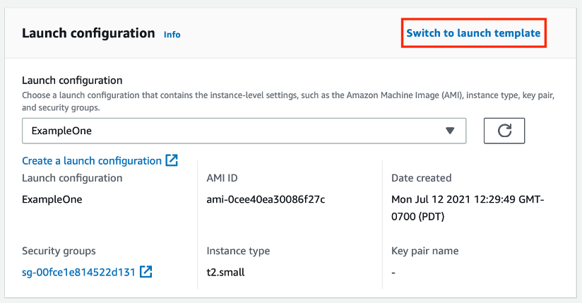
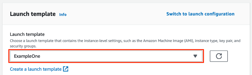
Clues about the type of workload running are useful for estimating the migration effort to Graviton. For some workloads, transitioning to Graviton is as simple as updating the instance types and associated Amazon Machine Images (AMIs) directly or in various launch or CloudFormation templates. For other workloads, you might need to use different software versions or change source codes. The quickest and easiest workloads to transition are Linux-based open-source applications. Many open source projects already support Arm64, and by extension Graviton. Therefore, many customers start their Graviton migration journey by checking whether their workloads are among the list of Graviton-compatible applications. They then combine this information with estimated savings from Compute Optimizer to build a list of Graviton migration opportunities.

Because Compute Optimizer cannot see into an instance, it looks to instance attributes for clues about the workload type running on the EC2 instance. The clues Compute Optimizer uses are based on the instance attributes customers provide, such as instance tags, AWS Marketplace product names, AMI names, and CloudFormation templates names. For example, when an instance is tagged with “key:application-type” and “value:hadoop”, Compute Optimizer will identify the application –Apache Hadoop in this example. Then, because we know that major frameworks, such as Apache Hadoop, Apache Spark, and many others, run on Graviton, Compute Optimizer will indicate that there is low migration effort to Graviton, and point customers to documentation that outlines the required steps for migrating a Hadoop application to Graviton.

As another example, when Compute Optimizer sees an instance is using a Microsoft Windows SQL Server AMI, Compute Optimizer will infer that SQL Server is running. Then, because it takes a lot of effort to modernize and migrate a SQL Server workload to Arm, Compute Optimizer will indicate that there is a high migration effort to Graviton. The most effective way to give Compute Optimizer clues about what application is running is by putting an “application-type” tag onto each instance. If Compute Optimizer doesn’t have enough clues, it will indicate that it doesn’t have enough information to offer migration guidance.

The following shows the different levels of migration effort:

  • Very Low – The recommended instance type has the same CPU architecture as the current instance type. Often, customers can just modify instance types directly, or do a simple re-deployment onto the new instance type. So, this is just an optimization, not a migration.
  • Low – The recommended instance type has different CPU architecture from the current instance type, but there’s a low-effort migration path. For example, migrating Apache Hadoop or Redis from x86 to Graviton falls under this category as both Hadoop and Redis have Graviton-compatible versions.
  • Medium – The recommended instance type has different CPU architecture from the current instance type, but Compute Optimizer doesn’t have enough information to offer migration guidance.
  • High – The recommended instance type has different CPU architecture from the current instance type, and the workload has no known compatible version on the recommended CPU architecture. Therefore, customers may need to re-compile their applications or re-platform their workloads (like moving from SQL Server to MySQL).

More and more applications support Graviton every day. If you’re running an application that you know has low migration effort, but Compute Optimizer isn’t yet aware, please tell us! Shoot us an email at [email protected] with the application type, and we’ll update our migration guidance mappings as quickly as we can. You can also put an “application-type” tag on your instances so that Compute Optimizer can infer your application type with high confidence.

Customers who have already opted into Compute Optimizer recommendations will have immediate access to this new capability. Customers who haven’t can opt-in with a single console click or API, enabling all Compute Optimizer features.

Walk through

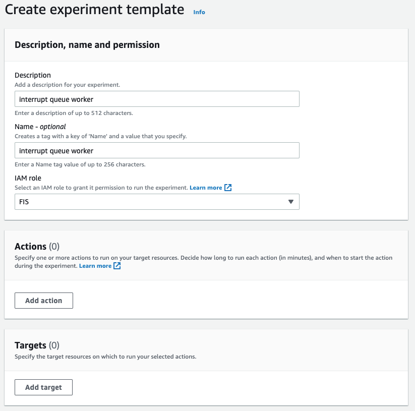
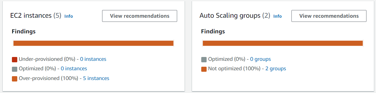
Now, let’s take a look at how to get started with Graviton recommendation on Compute Optimizer. When you open the Compute Optimizer console, you will see the dashboard page that provides you with a summary of all optimization opportunities in your account. Graviton recommendation is available for EC2 instances and Auto Scaling groups.

Screenshot of Compute Optimizer dashboard page, which shows the number of EC2 instance and Auto Scaling group recommendations by findings in your AWS account.

After you click on View recommendations for EC2 instances, you will come to the EC2 recommendation list view. Here is where you can see a list of your EC2 instances, their current instance type, our finding (over-provisioned, under-provisioned, or optimized), the recommended optimal instance type, and the estimated savings if there is a downsizing opportunity. By default, we will show you the best-fit instance type for the price regardless of CPU architecture. In many cases this means that Graviton will be recommended because EC2 offers a wide selection of Graviton instances with comparatively high price/performance ratio. If you’d like to only look at recommendations with your current architecture, you can use the CPU architecture preference dropdown to tell Compute Optimizer to show recommendations with only the current CPU architecture.

Compute Optimizer EC2 Recommendation List Page. Here you can select both current and Graviton as the preferred CPU architectures. The recommendation list contains two new columns -- migration effort, and inferred workload types.

Here you can see two new columns — Migration effort and Inferred workload types. The Inferred workload types field shows the type of workload Compute Optimizer has inferred your instance is running. The Migration effort field shows how much effort you might need to spend if you migrate from your current instance type to recommended instance type based on the inferred workload type. When there is no change in CPU architecture (i.e. moving from an x86-instance type to another x86-instance type, like in the third row), the migration effort will be Very low. For x86-instances that are running Graviton-compatible applications, such as Apache Hadoop, NGINX, Memcached, etc., when you migrate the instance to Graviton, the effort will be Low. If Compute Optimizer cannot identify the applications, the migration effort from x86 to Graviton will be Medium, and you can provide application type data by putting an application-type tag key onto the instance. You can click on each row to see more detailed recommendation. Let’s click on the first row.

Compute Optimizer EC2 Recommendation Detail Page. The current instance type is r5.large. Recommended option 1 is r6g.large, with low migration effort. Recommended option 2 is t4g.xlarge, with low migration effort. Recommended option 3 is m6g.xlarge, with low migration effort.

Compute Optimizer identifies this instance to be running Apache Hadoop workloads because there’s Amazon EMR system tag associated with it. It shows a banner that details why Compute Optimizer considers this as a low-effort Graviton migration candidate, and offers a migration guide when you click on Learn more.

Github screenshot of AWS Graviton migration guide. The migration guide details steps to transition workloads from x86-based instances to Graviton-based instances.

The same Graviton recommendation can also be retrieved through Compute Optimizer API or CLI. Here’s a sample CLI that retrieves the same recommendation as discussed above:

aws compute-optimizer get-ec2-instance-recommendations --instance-arns arn:aws:ec2:us-west-2:020796573343:instance/i-0b5ec1bb9daabf0f3 --recommendation-preferences "{\"cpuVendorArchitectures\": [\"CURRENT\" , \"AWS_ARM64\"]}"
{
    "instanceRecommendations": [
        {
            "instanceArn": "arn:aws:ec2:us-west-2:000000000000:instance/i-0b5ec1bb9daabf0f3",
            "accountId": "000000000000",
            "instanceName": "Compute Intensive",
            "currentInstanceType": "r5.large",
            "finding": "UNDER_PROVISIONED",
            "findingReasonCodes": [
                "CPUUnderprovisioned",
                "EBSIOPSOverprovisioned"
            ],
            "inferredWorkloadTypes": [
                "ApacheHadoop"
            ],
            "utilizationMetrics": [
                {
                    "name": "CPU",
                    "statistic": "MAXIMUM",
                    "value": 100.0
                },
                {
                    "name": "EBS_READ_OPS_PER_SECOND",
                    "statistic": "MAXIMUM",
                    "value": 0.0
                },
                {
                    "name": "EBS_WRITE_OPS_PER_SECOND",
                    "statistic": "MAXIMUM",
                    "value": 4.943333333333333
                },
                {
                    "name": "EBS_READ_BYTES_PER_SECOND",
                    "statistic": "MAXIMUM",
                    "value": 0.0
                },
                {
                    "name": "EBS_WRITE_BYTES_PER_SECOND",
                    "statistic": "MAXIMUM",
                    "value": 880541.9921875
                },
                {
                    "name": "NETWORK_IN_BYTES_PER_SECOND",
                    "statistic": "MAXIMUM",
                    "value": 18113.96638888889
                },
                {
                    "name": "NETWORK_OUT_BYTES_PER_SECOND",
                    "statistic": "MAXIMUM",
                    "value": 90.37638888888888
                },
                {
                    "name": "NETWORK_PACKETS_IN_PER_SECOND",
                    "statistic": "MAXIMUM",
                    "value": 2.484055555555556
                },
                {
                    "name": "NETWORK_PACKETS_OUT_PER_SECOND",
                    "statistic": "MAXIMUM",
                    "value": 0.3302777777777778
                }
            ],
            "lookBackPeriodInDays": 14.0,
            "recommendationOptions": [
                {
                    "instanceType": "r6g.large",
                    "projectedUtilizationMetrics": [
                        {
                            "name": "CPU",
                            "statistic": "MAXIMUM",
                            "value": 70.76923076923076
                        }
                    ],
                    "platformDifferences": [
                        "Architecture"
                    ],
                    "migrationEffort": "Low",
                    "performanceRisk": 1.0,
                    "rank": 1
                },
                {
                    "instanceType": "t4g.xlarge",
                    "projectedUtilizationMetrics": [
                        {
                            "name": "CPU",
                            "statistic": "MAXIMUM",
                            "value": 33.33333333333333
                        }
                    ],
                    "platformDifferences": [
                        "Hypervisor",
                        "Architecture"
                    ],
                    "migrationEffort": "Low",
                    "performanceRisk": 3.0,
                    "rank": 2
                },
                {
                    "instanceType": "m6g.xlarge",
                    "projectedUtilizationMetrics": [
                        {
                            "name": "CPU",
                            "statistic": "MAXIMUM",
                            "value": 33.33333333333333
                        }
                    ],
                    "platformDifferences": [
                        "Architecture"
                    ],
                    "migrationEffort": "Low",
                    "performanceRisk": 1.0,
                    "rank": 3
                }
            ],
            "recommendationSources": [
                {
                    "recommendationSourceArn": "arn:aws:ec2:us-west-2:000000000000:instance/i-0b5ec1bb9daabf0f3",
                    "recommendationSourceType": "Ec2Instance"
                }
            ],
            "lastRefreshTimestamp": "2021-12-28T11:00:03.576000-08:00",
            "currentPerformanceRisk": "High",
            "effectiveRecommendationPreferences": {
                "cpuVendorArchitectures": [
                    "CURRENT", 
                    "AWS_ARM64"
                ],
                "enhancedInfrastructureMetrics": "Inactive"
            }
        }
    ],
    "errors": []
}

Conclusion

Compute Optimizer Graviton recommendations are available in in US East (Ohio), US East (N. Virginia), US West (N. California), US West (Oregon), Asia Pacific (Mumbai), Asia Pacific (Seoul), Asia Pacific (Singapore), Asia Pacific (Sydney), Asia Pacific (Tokyo), Canada (Central), Europe (Frankfurt), Europe (Ireland), Europe (London), Europe (Paris), Europe (Stockholm), and South America (São Paulo) Regions at no additional charge. To get started with Compute Optimizer, visit the Compute Optimizer webpage.

Efficiently Scaling kOps clusters with Amazon EC2 Spot Instances

Post Syndicated from Pranaya Anshu original https://aws.amazon.com/blogs/compute/efficiently-scaling-kops-clusters-with-amazon-ec2-spot-instances/

This post is written by Carlos Manzanedo Rueda, WW SA Leader for EC2 Spot, and Brandon Wagner, Senior Software Development Engineer for EC2.

This post focuses on how you can leverage recently released tools to optimize your usage of Amazon EC2 Spot Instances on Kubernetes Operations (kOps) clusters. Spot Instances let you utilize unused capacity in the AWS cloud for up to 90% off compared to On-Demand prices, and they are a great fit for fault-tolerant, containerized applications. kOps is an open source project providing a cohesive toolset for provisioning, operating, and deleting Kubernetes clusters in the cloud.

Even with customers such as Snap Inc., Babylon Health, and Fidelity Investments telling us how Amazon Elastic Kubernetes Service (EKS) is essential for running their containerized workloads, we appreciate that there are scenarios where using Amazon EC2 instances and kOps are a viable alternative. At AWS, we understand “one size does not fit all.” While we encourage Kubernetes users to contribute their feedback to the AWS container roadmap so that we can improve our services, we also would like to reduce heavy lifting and simplify Spot best practices integration in kOps clusters.

To simplify the integration of Spot Instances in kOps clusters, in January of 2021 we introduced a new kops toolbox command: kops toolbox instance-selector. The utility is distributed as part of the standard kOps distribution. Moreover, it simplifies the creation of kOps Instance Groups by configuring them with full adherence to Spot Instances best practices.

Handling Spot interruption notifications in Kubernetes

Let’s quickly recap Spot best practices. Spot Instances perform exactly like any other EC2 Instances, except that in exchange for their discounted price, they can be interrupted with a two-minute warning when EC2 must reclaim capacity. Applications running on Spot can typically recover from transient interruptions by simply starting a new instance. Spot best practices involve measures such as diversifying into as many Spot capacity pools as possible, choosing the right Spot allocation strategy, and utilizing Spot integrated services. These handle the Spot Instances lifecycles for you. This blog post on handling Spot interruptions dives deeper into AWS’s EC2 Spot best practices.

In Kubernetes, to handle spot termination and rebalance recommendation events (both explained in this blog post on proactively managing Spot Instance lifecycle), we utilize the AWS open-source project AWS Node Termination Handler. We will be deploying the Node Termination Handler as a kOps managed addon, which simplifies its setup and configuration.

The Node Termination Handler ensures that the Kubernetes control plane responds appropriately to events that can make EC2 instances unavailable. It can be operated in two different modes: Instance Metadata Service (IMDS), deployed as a DaemonSet, or Queue Processor, deployed as a Deployment Controller. We recommend running it in Queue Processor mode. The Queue Processor controller continuously monitors an Amazon Simple Queue Service (SQS) queue for events received from Amazon EventBridge. This can lead to node termination in your cluster. When one of these events is received, the Node Termination Handler notifies the Kubernetes control plane to cordon and drain the node that is about to be interrupted. Then, the kubelet sends a SIGTERM signal to the Pods and containers running on the node. This lets your application proceed with a graceful termination – one of the recommended best practices of a Twelve-Factor App.

The kOps managed addon will let you configure the Node Termination Handler within your kOps cluster spec and, more importantly, manage provisioning the necessary infrastructure for you.

To deploy the AWS Node Termination Handler, we start by editing our cluster spec:

kops edit cluster --name ${KOPS_CLUSTER_NAME}

We append the nodeTerminationHandler configuration to the spec node:

spec:
  nodeTerminationHandler:
    enabled: true
    enableSQSTerminationDraining: true
    managedASGTag: "aws-node-termination-handler/managed"

Finally, we deploy the changes made to our cluster configuration:

kops update cluster --name ${KOPS_CLUSTER_NAME} –-state {KOPS_STATE_STORE} --yes --admin

${KOPS_CLUSTER_NAME} refers to the environment variable containing the cluster name, and ${KOPS_STATE_STORE} indicates the Amazon Simple Storage Service (S3) bucket – or kOps State Store – where kOps configuration is stored.

To check that your Node Termination Handler deployment was successful, you can execute:

kops get deployment aws-node-termination-handler -n kube-system

Instance Flexibility and Diversification

Diversification and selection of multiple instances types is essential to acquire and maintain Spot capacity, as well as to successfully replace interrupted instances with others from different pools. When running kOps on AWS, this is implemented by utilizing Amazon EC2 Auto Scaling. Amazon Auto Scaling group’s capacity-optimized allocation strategy ensures that Spot capacity is provisioned from the optimal pools, thereby reducing the chances of Spot terminations.

Simplifying adoption of Spot Best practices on kOps

Before the kops toolbox instance-selector, you would have to setup Spot best practices on kOps manually. This involved writing a stub file following the InstanceGroup specification and examples, and then implementing every best practice, including finding every pool that qualifies for our workload.

The new functionality in kops toolbox instance-selector simplifies InstanceGroup creation by moving the focus of kOps users and administrators from this manual configuration over to simply selecting the vCPUs and Memory requirements for their application (or a base instance type), and then letting kops toolbox instance-selector define the right configuration. Behind the scenes, it utilizes a library allowing it to plug into the feature-set of Amazon EC2 instance selector. At its core, ec2 instance selector helps you select compatible instance types for your application to run on. Utilize ec2 instance selector CLI or library when automating your configurations. In the case of kOps, the integration already comes in the kops toolbox.

For example, let’s say your cluster runs stateless, fault tolerant applications that are CPU/Memory bound and have a ratio of vCPU to Memory requiring at least 1vCPU : 4GB of RAM. You can run the following command in order to acquire cluster spot capacity:

kops toolbox instance-selector "spot-group-" \
  --usage-class spot --flexible --cluster-autoscaler \
  --vcpus-to-memory-ratio="1:4" \
  --ig-count 2

Let’s focus first on the command, and later cover its output. You can get a list of parameters and default values by running: kops toolbox instance-selector –help. A few default parameters weren’t passed in the command above, but they will be set to sane defaults, such as the maximum and minimum number of instances in the Instance Group. The parameter –flexible refers to our request to provide a group of flexible instance types spanning multiple generations.

Once you’ve defined the InstanceGroups, start them up by using the command:

kops update cluster \
–state=${KOPS_STATE_STORE} \
–name=${KOPS_CLUSTER_NAME} \
–yes –admin

The two commands above define and create a request for spot capacity from a flexible and diversified pool set, which meet the criteria to provide at least 4GB of RAM for each vCPU. The command creates not just one, but two node groups named “spot-group-1” and “spot-group-2” (–ig-count 2).

Now, let’s check the contents of the configuration file generated by kops toolbox instance-selector. To preview a configuration without making changes, add –dry-run –output yaml.

apiVersion: kops.k8s.io/v1alpha2
kind: InstanceGroup
metadata:
  creationTimestamp: "2020-08-11T10:22:16Z"
  labels:
    kops.k8s.io/cluster: spot-kops-cluster.k8s.local
  name: spot-group-1
spec:
  cloudLabels:
    k8s.io/cluster-autoscaler/enabled: "1"
    k8s.io/cluster-autoscaler/spot-kops-cluster.k8s.local: "1"
    kops.k8s.io/instance-selector: "1"
  image: 099720109477/ubuntu/images/hvm-ssd/ubuntu-focal-20.04-amd64-server-20200716
  machineType: m3.xlarge
  maxSize: 15
  minSize: 2
  mixedInstancesPolicy:
    instances:
    - m3.xlarge
    - m4.xlarge
    - m5.xlarge
    - m5a.xlarge
    - t2.xlarge
    - t3.xlarge
    onDemandAboveBase: 0
    onDemandBase: 0
    spotAllocationStrategy: capacity-optimized
  nodeLabels:
    kops.k8s.io/instancegroup: spot-group-1
  role: Node
  subnets:
  - eu-west-1a
  - eu-west-1b
  - eu-west-1c
...

The configuration above lists one of the groups created by kops toolbox instance-selector in the previous example. The second group will have a very similar make-up and format, except that it will refer to instances such as: r3.xlarge, r4.xlarge, r5.xlarge, and r5a.xlarge in the mixedInstancesPolicy section. By defining the parameter –usage-class to Spot, the configuration created by kops toolbox instance-selector will add the tags identifying this Auto Scaling group as a Spot group. When the nodes are initialized, kOps controller will identify the nodes as Spot and add the label node-role.kubernetes.io/spot-worker=true. Therefore, at a later stage, we can apply placement logic to our cluster by using nodeSelector and affinity. The configuration above adheres to the definition of kOps support for mixed Instance Groups in AWS, and adds all of the right cloudLabels in order to integrate and implement not only with Spot best practices, but also with Cluster Autoscaler Auto-Discovery configuration best practices.

Kubernetes Cluster Autoscaler is a Kubernetes controller that dynamically adjusts the cluster size. According to a 2020 survey by Cloud Native Computing Foundation (CNCF), 70% of Kubernetes workloads plan to autoscale their stateless applications. Dynamically scaling applications and clusters is also a great practice for optimizing your system costs in situations where capacity is unnecessary, as well as for scaling out accordingly in order to meet business demands. If there are Pods that can’t be scheduled due to insufficient resources, then Cluster Autoscaler will issue a Scale-out action. When there are nodes in the cluster that have been under-utilized for a configurable period of time, Cluster Autoscaler will Scale-in the cluster, and even down-scale to 0 instances when applications don’t need to be run.

On Scale-out operations, Cluster Autoscaler evaluates a set of node groups. When Cluster Autoscaler runs on AWS, node groups are implemented by using Auto Scaling groups (referring to the same instance group as a kOps Instance Group). Therefore, to calculate the number of nodes to scale-out, Cluster Autoscaler assumes that every instance in a node group has the same number of vCPUs and memory size.

By creating two node groups, you apply two diversification levels. You diversify within each node group by using an Auto Scaling group with Mixed Instance Policies and capacity-optimized allocation strategy. Then, to increase the pool range you can leverage, you add more than one node group, while still adhering to the best practices required by Cluster Autoscaler.

While we’ve been focusing on Spot Instances, the parameter –usage-class can be utilized to get OnDemand instances instead of Spot. In the next example, let’s say we would like to get On-Demand capacity in order to train complex deep learning models that will take hours to run. To train our models, we need instances that have at least one GPU with 16GB of RAM on instances that have at least 32GB Ram and 8 vCPUs.

kops toolbox instance-selector "ondemand-gpu-group" \
  --gpus-min 1 --gpu-memory-total-min 16gb --memory-min 32gb --vcpus 8\
  --node-count-max 4 --node-count-min 4 --cpu-architecture amd64

The command above, followed by kops update cluster –state=${KOPS_STATE_STORE} –name=${KOPS_CLUSTER_NAME} –yes can be utilized to produce a configuration and create a nodegroup with the right requirements. This could be created at the start of the training procedure, and then – once the training is done and the capacity is no longer needed – you could automate the nodegroup removal with the following command:

kops delete instancegroup ondemand-gpu-group --name ${KOPS_CLUSTER_NAME} –yes

Conclusions

We believe the best way to run Kubernetes on AWS is by using Amazon EKS. However, scenarios may exist where kOps is utilized in AWS. By using the kOps managed add-on to install aws-node-termination-handler and kops toolbox instance-selector, it is easier than ever to apply Spot best practices to Kubernetes workloads on kOps, and cost-optimize fault-tolerant, stateless applications. These tools let kOps workloads gracefully terminate applications, as well as proactively handle the replacement of instances that are at an elevated risk of termination. kops toolbox instance-selector leverages Amazon ec2-instance-selector in order to simplify the creation of Instance Group configurations adhering to Spot Instances best practices, implementing instance type flexibility, and utilizing capacity-optimized allocation strategy.

By adhering to these best practices to reduce the frequency of Spot interruptions, we will optimize not only the cost, but also our Spot Instances selection. This will enable us to acquire capacity at a massive scale if necessary.

To start using the tools we have described, follow along this step-by-step tutorial. Also, head over to the kops toolbox documentation to learn more about the ways in which you can use it.

Using EC2 Auto Scaling predictive scaling policies with Blue/Green deployments

Post Syndicated from Pranaya Anshu original https://aws.amazon.com/blogs/compute/retaining-metrics-across-blue-green-deployment-for-predictive-scaling/

This post is written by Ankur Sethi, Product Manager for EC2.

Amazon EC2 Auto Scaling allows customers to realize the elasticity benefits of AWS by automatically launching and shutting down instances to match application demand. Earlier this year we introduced predictive scaling, a new EC2 Auto Scaling policy that predicts demand and proactively scales capacity, resulting in better availability of your applications (if you are new to predictive scaling, I suggest you read this blog post before proceeding). In this blog, I will walk you through how to use a new feature, predictive scaling custom metrics, to configure predictive scaling for an application that follows a Blue/Green deployment strategy.

Blue/Green Deployment using Auto Scaling groups

The fundamental idea behind Blue/Green deployment is to shift traffic between two environments that are running different versions of your application. The Blue environment represents your current application version serving production traffic. In parallel, the Green environment is staged running the newer version. After the Green environment is ready and tested, production traffic is redirected from Blue to Green either all at once or in increments, similar to canary deployments. At the end of the load transfer, you can either terminate the Blue Auto Scaling group or reuse it to stage the next version update. Irrespective of the approach, when a new Auto Scaling group is created as part of Blue/Green deployment, EC2 Auto Scaling, and in turn predictive scaling, does not know that this new Auto Scaling group is running the same application that the Blue one was. Predictive scaling needs a minimum of 24 hours of historical metric data and up to 14 days for the most accurate results, neither of which the new Auto Scaling group has when the Blue/Green deployment is initiated. This means that if you frequently conduct Blue/Green deployments, predictive scaling regularly pauses for at least 24 hours, and you may experience less optimal forecasts after each deployment.

In Blue/Green deployment you have two Auto Scaling groups - Blue Auto Scaling Group running the current version and Green Auto Scaling group staged with the updated version. Once you are ready to make the updated version live, you switch production traffic from Blue to Green through your load balancer or your DNS settings.

Figure 1. In Blue/Green deployment you have two Auto Scaling groups running different versions of an application. You switch production traffic from Blue to Green to make the updated version public.

How to retain your application load history using predictive scaling custom metrics

To make predictive scaling work for Blue/Green deployment scenarios, we need to aggregate load metrics from both Blue and Green environments before using it to forecast capacity as depicted in the following illustration. The key benefit of using the aggregated metric is that, throughout the Blue/Green deployment, predictive scaling can continue to forecast load correctly without a pause, and it can retain the entire 14 days of data to provide the best predictions. For example, if your application observes different patterns during a weekday vs. a weekend, predictive scaling will be able to retain knowledge of that pattern after the deployment.

The aggregated metrics of Blue and Green Auto Scaling groups give you the total load traffic of an application. Prior to Blue/Green deployment, Blue Auto Scaling group served the entire traffic while after the deployment, Green Auto Scaling group handles it. There can be a period of overlap where traffic is split between the two Auto Scaling groups. By adding the traffic on two Auto Scaling groups, you get a single time series which allows predictive scaling to generate forecasts based on complete set of 14 days of history.

Figure 2. The aggregated metrics of Blue and Green Auto Scaling groups give you the total load traffic of an application. Predictive scaling gives most accurate forecasts when based on last 14 days of history.

Example

Let’s explore this solution with an example. I created a sample application and load simulation infrastructure that you can use to follow along by deploying this example AWS CloudFormation Stack in your account. This example deploys two Auto Scaling groups: ASG-myapp-v1 (Blue) and ASG-myapp-v2 (Green) to run a sample application. Only ASG-myapp-v1 is attached to a load balancer and has recurring requests generated for its application. I have applied a target tracking policy and predictive scaling policy to maintain CPU utilization at 25%. You should keep this Auto Scaling group running for at least 24 hours before proceeding with the rest of the example to have enough load generated for predictive scaling to start forecasting.

ASG-myapp-v2 does not have any requests generated of its own. In the following sections, to highlight how metric aggregation works, I will apply a predictive scaling policy to it using Custom Metric configurations aggregating CPU Utilization metrics of both Auto Scaling groups. I’ll then verify if the forecasts are generated for ASG-myapp-v2 based on the aggregated metrics.

As part of your Blue/Green deployment approach, if you alternate between exactly two Auto Scaling groups, then you can use simple math expressions such as SUM (m1, m2) where m1 and m2 are metrics for each Auto Scaling group. However, if you create new Auto Scaling groups for each deployment, then you need to refer to the metrics of all the Auto Scaling groups that were used to run the application in the last 14 days. You can simplify this task by following a naming convention for your Auto Scaling groups and leveraging the Search expression to select the required metrics. The naming convention is ASG-myapp-vx where we name the new Auto Scaling group according to the version number (ASG-myapp-v1ASG-myapp-v2 and so on). Using SEARCH(‘ {Namespace, DimensionName1, DimensionName2} SearchTerm’, ‘Statistic’, Period) expression I can identify the metrics of all the Auto Scaling groups that follow the name according to the SearchTerm. I can then aggregate the metrics by appending another expression. The final expression should look like SUM(SEARCH(…).

Step 1: Apply predictive scaling policy to Green Auto Scaling group ASG-myapp-v2 with custom metrics

To generate forecasts, the predictive scaling algorithm needs three metrics as input: a load metric that represents total demand on an Auto Scaling group, the number of instances that represents the capacity of the Auto Scaling groups, and a scaling metric that represents the average utilization of the instances in the Auto Scaling groups.

Here is how it would work with CPU Utilization metrics. First, create a scaling configuration file where you define the metrics, target value, and the predictive scaling mode for your policy.

cat predictive-scaling-policy-cpu.json
{
        "MetricSpecifications": [
      {
            "TargetValue": 25,
           "CustomizedLoadMetricSpecification": {
        },
           "CustomizedCapacityMetricSpecification": {  
        },
           "CustomizedScalingMetricSpecification": {
        },
            }
    ],
        "Mode": “ForecastOnly”
}
EoF

I’ll elaborate on each of these metric specifications separately in the following sections. You can download the complete JSON file in GitHub.

Customized Load Metric Specification: You can aggregate the demand across your Auto Scaling groups by using the SUM expression. The demand forecasts are generated every hour, so this metric has to be aggregated with a time period of 3600 seconds.

"CustomizedLoadMetricSpecification": {
    "MetricDataQueries": [
        {
            "Id": "load_sum",
            "Expression": "SUM(SEARCH('{AWS/EC2,AutoScalingGroupName} MetricName=\"CPUUtilization\" ASG-myapp', 'Sum', 3600))"
        }
    ]
}

Customized Capacity Metric Specification: Your customized capacity metric represents the total number of instances across your Auto Scaling groups. Similar to the load metric, the aggregation across Auto Scaling groups is done by using the SUM expression. Note that this metric has to follow a 300 seconds interval period.

"CustomizedCapacityMetricSpecification": {
    "MetricDataQueries": [
        {
            "Id": "capacity_sum",
            "Expression": "SUM(SEARCH('{AWS/AutoScaling,AutoScalingGroupName} MetricName=\"GroupInServiceIntances\" ASG-myapp', 'Average', 300))"
        }
    ]
}

Customized Scaling Metric Specification: Your customized scaling metric represents the average utilization of the instances across your Auto Scaling groups. We cannot simply SUM the scaling metric of each Auto Scaling group as the utilization is an average metric that depends on the capacity and demand of the Auto Scaling group. Instead, we need to find the weighted average unit load (Load Metric/Capacity). To do so, we will use an expression: Sum(load)/Sum(capacity). Note that this metric also has to follow a 300 seconds interval period.

"CustomizedScalingMetricSpecification": {
    "MetricDataQueries": [
        {
            "Id": "capacity_sum",
            "Expression": "SUM(SEARCH('{AWS/AutoScaling,AutoScalingGroupName} MetricName=\"GroupInServiceIntances\" ASG-myapp', 'Average', 300))"
            “ReturnData”: “False”
        },
        {
            "Id": "load_sum",
            "Expression": "SUM(SEARCH('{AWS/EC2,AutoScalingGroupName} MetricName=\"CPUUtilization\" ASG-myapp', 'Sum', 300))"
            “ReturnData”: “False”
        },
        {
            "Id": "weighted_average",
            "Expression": "load_sum / capacity_sum”
       }
    ]
}

Once you have created the configuration file, you can run the following CLI command to add the predictive scaling policy to your Green Auto Scaling group.

aws autoscaling put-scaling-policy \
    --auto-scaling-group-name "ASG-myapp-v2" \
    --policy-name "CPUUtilizationpolicy" \
    --policy-type "PredictiveScaling" \
    --predictive-scaling-configuration file://predictive-scaling-policy-cpu.json

Instantaneously, the forecasts will be generated for the Green Auto Scaling group (My-ASG-v2) as if this new Auto Scaling group has been running the application. You can validate this using the predictive scaling forecasts API. You can also use the console to review forecasts by navigating to the Amazon EC2 Auto Scaling console, selecting the Auto Scaling group that you configured with predictive scaling, and viewing the predictive scaling policy located under the Automatic Scaling section of the Auto Scaling group details view.

EC2 Auto Scaling console shows you the capacity and load forecasts generated by your predictive scaling policies against the actual metric values. In this case, we are looking at the forecasts generated for Green Auto Scaling group. Since we aggregated metrics across Auto Scaling groups, the forecasts are generated as if this Auto Scaling group has been running the application from the beginning. You see the actual load and capacity values also aggregated for easier comparison of the forecasted and actual values.

Figure 3. EC2 Auto Scaling console showing capacity and load forecasts for Green Auto Scaling group. The forecasts are generated as if this Auto Scaling group has been running the application from the beginning.

Step 2: Terminate ASG-myapp-v1 and see predictive scaling forecasts continuing

Now complete the Blue/Green deployment pattern by terminating the Blue Auto Scaling group, and then go to the console to check if the forecasts are retained for the Green Auto Scaling group.

aws autoscaling delete-auto-scaling-group \
 --auto-scaling-group-name ASG-myapp-v1

You can quickly check the forecasts on the console for ASG-myapp-v2 to find that terminating the Blue Auto Scaling group has no impact on the forecasts of the Green one. The forecasts are all based on aggregated metrics. As you continue to do Blue/Green deployments in future, the history of all the prior Auto Scaling groups will persist, ensuring that our predictions are always based on the complete set of metric history. Before we conclude, remember to delete the resources you created. As part of this example, to avoid unnecessary costs, delete the CloudFormation stack.

Conclusion

Custom metrics give you the flexibility to base predictive scaling on metrics that most accurately represent the load on your Auto Scaling groups. This blog focused on the use case where we aggregated metrics from different Auto Scaling groups across Blue/Green deployments to get accurate forecasts from predictive scaling. You don’t have to wait for 24 hours to get the first set of forecasts or manually set capacity when the new Auto Scaling group is created to deploy an updated version of the application. You can read about other use cases of custom metrics and metric math in the public documentation such as scaling based on queue metrics.

Implementing interruption tolerance in Amazon EC2 Spot with AWS Fault Injection Simulator

Post Syndicated from Pranaya Anshu original https://aws.amazon.com/blogs/compute/implementing-interruption-tolerance-in-amazon-ec2-spot-with-aws-fault-injection-simulator/

This post is written by Steve Cole, WW SA Leader for EC2 Spot, and David Bermeo, Senior Product Manager for EC2.

On October 20, 2021, AWS released new functionality to the Amazon Fault Injection Simulator that supports triggering the interruption of Amazon EC2 Spot Instances. This functionality lets you test the fault tolerance of your software by interrupting instances on command. The triggered interruption will be preceded with a Rebalance Recommendation (RBR) and Instance Termination Notification (ITN) so that you can fully test your applications as if an actual Spot interruption had occurred.

In this post, we’ll provide two examples of how easy it has now become to simulate Spot interruptions and validate the fault-tolerance of an application or service. We will demonstrate testing an application through the console and a service via CLI.

Engineering use-case (console)

Whether you are building a Spot-capable product or service from scratch or evaluating the Spot compatibility of existing software, the first step in testing is identifying whether or not the software is tolerant of being interrupted.

In the past, one way this was accomplished was with an AWS open-source tool called the Amazon EC2 Metadata Mock. This tool let customers simulate a Spot interruption as if it had been delivered through the Instance Metadata Service (IMDS), which then let customers test how their code responded to an RBR or an ITN. However, this model wasn’t a direct plug-and-play solution with how an actual Spot interruption would occur, since the signal wasn’t coming from AWS. In particular, the method didn’t provide the centralized notifications available through Amazon EventBridge or Amazon CloudWatch Events that enabled off-instance activities like launching AWS Lambda functions or other orchestration work when an RBR or ITN was received.

Now, Fault Injection Simulator has removed the need for custom logic, since it lets RBR and ITN signals be delivered via the standard IMDS and event services simultaneously.

Let’s walk through the process in the AWS Management Console. We’ll identify an instance that’s hosting a perpetually-running queue worker that checks the IMDS before pulling messages from Amazon Simple Queue Service (SQS). It will be part of a service stack that is scaled in and out based on the queue depth. Our goal is to make sure that the IMDS is being polled properly so that no new messages are pulled once an ITN is received. The typical processing time of a message with this example is 30 seconds, so we can wait for an ITN (which provides a two minute warning) and need not act on an RBR.

First, we go to the Fault Injection Simulator in the AWS Management Console to create an experiment.

AWS Fault Injection Simulator start screen in AWS Management console

At the experiment creation screen, we start by creating an optional name (recommended for console use) and a description, and then selecting an IAM Role. If this is the first time that you’ve used Fault Injection Simulator, then you’ll need to create an IAM Role per the directions in the FIS IAM permissions documentation. I’ve named the role that we created ‘FIS.’ After that, I’ll select an action (interrupt) and identify a target (the instance).

Experiment template screen in AWS Management console with description “interrupt queue worker,” name “interrupt queue worker,” and IAM role “FIS.”

First, I name the action. The Action type I want is to interrupt the Spot Instance: aws:ec2:send-spot-instance-interruptions. In the Action parameters, we are given the option to set the duration. The minimum value here is two minutes, below which you will receive an error since Spot Instances will always receive a two minute warning. The advantage here is that, by setting the durationBeforeInterruption to a value above two minutes, you will get the RBR (an optional point for you to respond) and ITN (the actual two minute warning) at different points in time, and this lets you respond to one or both.

New action form in the create experiment template screen with name, description, action type and durationBeforeInterruption fields filled.

The target instance that we launched is depicted in the following screenshot. It is a Spot Instance that was launched as a persistent request with its interruption action set to ‘stop’ instead of ‘terminate.’ The option to stop a Spot Instance, introduced in 2020, will let us restart the instance, log in and retrieve logs, update code, and perform other work necessary to implement Spot interruption handling.

Now that an action has been defined, we configure the target. We have the option of naming the target, which we’ve done here to match the Name tagged on the EC2 instance ‘qWorker’. The target method we want to use here is Resource ID, and then we can either type or select the desired instance from a drop-down list. Selection mode will be ‘all’, as there is only one instance. If we were using tags, which we will in the next example, then we’d be able to select a count of instances, up to five, instead of just one.

Edit target form in the create experiment template screen with name, resource type, and resource id fields filled. Name is “qWorker,” Resource type is “aws:ec2:spot-Instance,” Target method is “Resource IDs” Resource IDs is “i-019ea405f8f81742b” and Selection mode is “All.”

Once you’ve saved the Action, the Target, and the Experiment, then you’ll be able to begin the experiment by selecting the ‘Start from the Action’ menu at the top right of the screen.

Fault Injection Simulator Experiment template summary screen in the AWS Management console highlights experiment template ID, stop conditions, description, creation time, IAM role, and last update time.

After the experiment starts, you’ll be able to observe its state by refreshing the screen. Generally, the process will take just seconds, and you should be greeted by the Completed state, as seen in the following screenshot.

Fault Injection Simulator Experiment summary screen in the AWS Management console shows status as “Completed.”

In the following screenshot, having opened an interruption log group created in CloudWatch Event Logs, we can see the JSON of the RBR.

CloudWatch Event Logs screen in the AWS Management Console with information on the EC2 Rebalance Recommendation.

Two minutes later, we see the ITN in the same log group.

Cloudwatch Event Logs screen in the AWS Management console with information on the Instance Termination Notification.

Another two minutes after the ITN, we can see the EC2 instance is in the process of stopping (or terminating, if you elect).

EC2 Instance List screen in the AWS Management console with information on the instance that is stopping.

Shortly after the stop is issued by EC2, we can see the instance stopped. It would now be possible to restart the instance and view logs, make code changes, or do whatever you find necessary before testing again.

EC2 Instance List screen in the AWS Management console with information on the Instance that is stopped.

Now that our experiment succeeded in interrupting our Spot Instance, we can evaluate the performance of the code running on the instance. It should have completed the processing of any messages already retrieved at the ITN, and it should have not pulled any new messages afterward.

This experiment can be saved for later use, but it will require selecting the specific instance each time that it’s run. We can also re-use the experiment template by using tags instead of an instance ID, as we’ll show in the next example. This shouldn’t prove troublesome for infrequent experiments, and especially those run through the console. Or, as we did in our example, you can set the instance interruption behavior to stop (versus terminate) and re-use the experiment as long as that particular instance continues to exist. When the experiments get more frequent, it might be advantageous to automate the process, possibly as part of the test phase of a CI/CD pipeline. Doing this is programmatically possible through the AWS CLI or SDK.

Operations use-case (CLI)

Once the developers of our product validate the single-instance fault tolerance, indicating that the target workload is capable of running on Spot Instances, then the next logical step is to deploy the product as a service on multiple instances. This will allow for more comprehensive testing of the service as a whole, and it is a key process in collecting valuable information, such as performance data, response times, error rates, and other metrics to be used in the monitoring of the service. Once data has been collected on a non-interrupted deployment, it is then possible to use the Spot interruption action of the Fault Injection Simulator to observe how well the service can handle RBR and ITN while running, and to see how those events influence the metrics collected previously.

When testing a service, whether it is launched as instances in an Amazon EC2 Auto Scaling group, or it is part of one of the AWS container services, such as Amazon Elastic Container Service (Amazon ECS) or the Amazon Elastic Kubernetes Service (EKS), EC2 Fleet, Amazon EMR, or across any instances with descriptive tagging, you now have the ability to trigger Spot interruptions to as many as five instances in a single Fault Injection Simulator experiment.

We’ll use tags, as opposed to instance IDs, to identify candidates for interruption to interrupt multiple Spot Instances simultaneously. We can further refine the candidate targets with one or more filters in our experiment, for example targeting only running instances if you perform an action repeatedly.

In the following example, we will be interrupting three instances in an Auto Scaling group that is backing a self-managed EKS node group. We already know the software will behave as desired from our previous engineering tests. Our goal here is to see how quickly EKS can launch replacement tasks and identify how the service as a whole responds during the event. In our experiment, we will identify instances that contain the tag aws:autoscaling:groupName with a value of “spotEKS”.

The key benefit here is that we don’t need a list of instance IDs in our experiment. Therefore, this is a re-usable experiment that can be incorporated into test automation without needing to make specific selections from previous steps like collecting instance IDs from the target Auto Scaling group.

We start by creating a file that describes our experiment in JSON rather than through the console:

{
    "description": "interrupt multiple random instances in ASG",
    "targets": {
        "spotEKS": {
            "resourceType": "aws:ec2:spot-instance",
            "resourceTags": {
                "aws:autoscaling:groupName": "spotEKS"
            },
            "selectionMode": "COUNT(3)"
        }
    },
    "actions": {
        "interrupt": {
            "actionId": "aws:ec2:send-spot-instance-interruptions",
            "description": "interrupt multiple instances",
            "parameters": {
                "durationBeforeInterruption": "PT4M"
            },
            "targets": {
            "SpotInstances": "spotEKS"
            }
        }
    },
    "stopConditions": [
        {
            "source": "none"
        }
    ],
    "roleArn": "arn:aws:iam::xxxxxxxxxxxx:role/FIS",
    "tags": {
        "Name": "multi-instance"
    }
}

Then we upload the experiment template to Fault Injection Simulator from the command-line.

aws fis create-experiment-template --cli-input-json file://experiment.json

The response we receive returns our template along with an ID, which we’ll need to execute the experiment.

{
    "experimentTemplate": {
        "id": "EXT3SHtpk1N4qmsn",
        ...
    }
}

We then execute the experiment from the command-line using the ID that we were given at template creation.

aws fis start-experiment --experiment-template-id EXT3SHtpk1N4qmsn

We then receive confirmation that the experiment has started.

{
    "experiment": {
        "id": "EXPaFhEaX8GusfztyY",
        "experimentTemplateId": "EXT3SHtpk1N4qmsn",
        "state": {
            "status": "initiating",
            "reason": "Experiment is initiating."
        },
        ...
    }
}

To check the status of the experiment as it runs, which for interrupting Spot Instances is quite fast, we can query the experiment ID for success or failure messages as follows:

aws fis get-experiment --id EXPaFhEaX8GusfztyY

And finally, we can confirm the results of our experiment by listing our instances through EC2. Here we use the following command-line before and after execution to generate pre- and post-experiment output:

aws ec2 describe-instances --filters\
 Name='tag:aws:autoscaling:groupName',Values='spotEKS'\
 Name='instance-state-name',Values='running'\
 | jq .Reservations[].Instances[].InstanceId | sort

We can then compare this to identify which instances were interrupted and which were launched as replacements.

< "i-003c8d95c7b6e3c63"
< "i-03aa172262c16840a"
< "i-02572fa37a61dc319"
---
> "i-04a13406d11a38ca6"
> "i-02723d957dc243981"
> "i-05ced3f71736b5c95"

Summary

In the previous examples, we have demonstrated through the console and command-line how you can use the Spot interruption action in the Fault Injection Simulator to ascertain how your software and service will behave when encountering a Spot interruption. Simulating Spot interruptions will help assess the fault-tolerance of your software and can assess the impact of interruptions in a running service. The addition of events can enable more tooling, and being able to simulate both ITNs and RBRs, along with the Capacity Rebalance feature of Auto scaling groups, now matches the end-to-end experience of an actual AWS interruption. Get started on simulating Spot interruptions in the console.

Identifying optimal locations for flexible workloads with Spot placement score

Post Syndicated from Pranaya Anshu original https://aws.amazon.com/blogs/compute/identifying-optimal-locations-for-flexible-workloads-with-spot-placement-score/

This post is written by Jessie Xie, Solutions Architect for EC2 Spot, and Peter Manastyrny, Senior Product Manager for EC2 Auto Scaling and EC2 Fleet.

Amazon EC2 Spot Instances let you run flexible, fault-tolerant, or stateless applications in the AWS Cloud at up to a 90% discount from On-Demand prices. Since we introduced Spot Instances back in 2009, we have been building new features and integrations with a single goal – to make Spot easy and efficient to use for your flexible compute needs.

Spot Instances are spare EC2 compute capacity in the AWS Cloud available for steep discounts. In exchange for the discount, Spot Instances are interruptible and must be returned when EC2 needs the capacity back. The location and amount of spare capacity available at any given moment is dynamic and changes in real time. This is why Spot workloads should be flexible, meaning they can utilize a variety of different EC2 instance types and can be shifted in real time to where the spare capacity currently is. You can use Spot Instances with tools such as EC2 Fleet and Amazon EC2 Auto Scaling which make it easy to run workloads on multiple instance types.

The AWS Cloud spans 81 Availability Zones across 25 Regions with plans to launch 21 more Availability Zones and 7 more Regions. However, until now there was no way to find an optimal location (either a Region or Availability Zone) to fulfill your Spot capacity needs without trying to launch Spot Instances there first. Today, we are excited to announce Spot placement score, a new feature that helps you identify an optimal location to run your workloads on Spot Instances. Spot placement score recommends an optimal Region or Availability Zone based on the amount of Spot capacity you need and your instance type requirements.

Spot placement score is useful for workloads that could potentially run in a different Region. Additionally, because the score takes into account your instance type selection, it can help you determine if your request is sufficiently instance type flexible for your chosen Region or Availability Zone.

How Spot placement score works

To use Spot placement score you need to specify the amount of Spot capacity you need, what your instance type requirements are, and whether you would like a recommendation for a Region or a single Availability Zone. For instance type requirements, you can either provide a list of instance types, or the instance attributes, like the number of vCPUs and amount of memory. If you choose to use the instance attributes option, you can then use the same attribute configuration to request your Spot Instances in the recommended Region or Availability Zone with the new attribute-based instance type selection feature in EC2 Fleet or EC2 Auto Scaling.

Spot placement score provides a list of Regions or Availability Zones, each scored from 1 to 10, based on factors such as the requested instance types, target capacity, historical and current Spot usage trends, and time of the request. The score reflects the likelihood of success when provisioning Spot capacity, with a 10 meaning that the request is highly likely to succeed. Provided scores change based on the current Spot capacity situation, and the same request can yield different scores when ran at different times. It is important to note that the score serves as a guideline, and no score guarantees that your Spot request will be fully or partially fulfilled.

You can also filter your score by Regions or Availability Zones, which is useful for cases where you can use only a subset of AWS Regions, for example any Region in the United States.

Let’s see how Spot placement score works in practice through an example.

Using Spot placement score with AWS Management Console

To try Spot placement score, log into your AWS account, select EC2, Spot Requests, and click on Spot placement score to open the Spot placement score window.

Spot placement score screen in AWS Management Console.

Here, you need provide your target capacity and instance type requirements by clicking on Enter requirements. You can enter target capacity as a number of instances, vCPUs, or memory. vCPUs and memory options are useful for vertically scalable workloads that are sized for a total amount of compute resources and can utilize a wide range of instance sizes. Target capacity is limited and based on your recent Spot usage with accounting for potential usage growth. For accounts that do not have recent Spot usage, there is a default limit aligned with the Spot Instances limit.

For instance type requirements, there are two options. First option is to select Specify instance attributes that match your compute requirements tab and enter your compute requirements as a number of vCPUs, amount of memory, CPU architecture, and other optional attributes. Second option is to select Manually select instance types tab and select instance types from the list.

Please note that you need to select at least three different instance types (that is, different families, generations, or sizes). If you specify a smaller number of instance types, Spot placement score will always yield a low score. Spot placement score is designed to help you find an optimal location to request Spot capacity tailored to your specific workload needs, but it is not intended to be used for getting high-level Spot capacity information across all Regions and instance types.

Let’s try to find an optimal location to run a workload that can utilize r5.8xlarge, c5.9xlarge, and m5.8xlarge instance types and is sized at 2000 instances.

Spot placement score screen in AWS Management Console with selected target capacity at 2000 instances and selected r5.8xlarge, c5.9xlarge, and m5.8xlarge instance types..

Once you select 2000 instances under Target capacity, select r5.8xlarge, c5.9xlarge, and m5.8xlarge instances under Select instance types, and click Load placement score button, you will get a list of Regions sorted by score in a descending order. There is also an option to filter by specific Regions if needed.

The highest rated Region for your requirements turns out to be US East (N. Virginia) with a score of 8. The second closest contender is Europe (Ireland) with a score of 5. That tells you that right now the optimal Region for your Spot requirements is US East (N. Virginia).

Spot placement score screen in AWS Management Console with displayed scores on Region level scores.

Let’s now see if it is possible to get a higher score. Remember, the key best practice for Spot is to be flexible and utilize as many instance types as possible. To do that, press the Edit button on the Target capacity and instance type requirements tab. For the new request, keep the same target capacity at 2000, but expand the selection of instance types by adding similarly sized instance types from a variety of instance families and generations, i.e., r5.4xlarge, r5.12xlarge, m5zn.12xlarge, m5zn.6xlarge, m5n.8xlarge, m5dn.8xlarge, m5d.8xlarge, r5n.8xlarge, r5dn.8xlarge, r5d.8xlarge, c5.12xlarge, c5.4xlarge, c5d.12xlarge, c5n.9xlarge. c5d.9xlarge, m4.4xlarge, m4.16xlarge, m4.10xlarge, r4.8xlarge, c4.8xlarge.

After requesting the scores with updated requirements, you can see that even though the score in US East (N. Virginia) stays unchanged at 8, the scores for Europe (Ireland) and US West (Oregon) improved dramatically, both raising to 9. Now, you have a choice of three high-scored Regions to request your Spot Instances, each with a high likelihood to succeed.

To request Spot Instances based on the score, you can use EC2 Fleet or EC2 Auto Scaling. Please note, that the score implies that you use capacity-optimized Spot allocation strategy when requesting the capacity. If you use other allocation strategies, such as lowest-price, the result in the recommended Region or Availability Zone will not align with the score provided.

Spot placement score screen in AWS Management Console with selected target capacity at 2000 instances and selected r5.8xlarge, c5.9xlarge, m5.8xlarge, r5.4xlarge, r5.12xlarge, m5zn.12xlarge, m5zn.6xlarge, m5n.8xlarge, m5dn.8xlarge, m5d.8xlarge, r5n.8xlarge, r5dn.8xlarge, r5d.8xlarge, c5.12xlarge, c5.4xlarge, c5d.12xlarge, c5n.9xlarge. c5d.9xlarge, m4.4xlarge, m4.16xlarge, m4.10xlarge, r4.8xlarge, c4.8xlarge instance types.

You can also request the scores at the Availability Zone level. This is useful for running workloads that need to have all instances in the same Availability Zone, potentially to minimize inter-Availability Zone data transfer costs. Workloads such as Apache Spark, which involve transferring a high volume of data between instances, would be a good use case for this. To get scores per Availability Zone you can check the box Provide placement scores per Availability Zone.

When requesting instances based on Availability Zone recommendation, you need to make sure to configure EC2 Fleet or EC2 Auto Scaling request to only use that specific Availability Zone.

With Spot placement score, you can test different instance type combinations at different points in time, and find the most optimal Region or Availability Zone to run your workloads on Spot Instances.

Availability and pricing

You can use Spot placement score today in all public and AWS GovCloud Regions with the exception of those based in China, where we plan to release later. You can access Spot placement score using the AWS Command Line Interface (CLI), AWS SDKs, and Management Console. There is no additional charge for using Spot placement score, you will only pay EC2 standard rates if provisioning instances based on recommendation.

To learn more about using Spot placement score, visit the Spot placement score documentation page. To learn more about best practices for using Spot Instances, see Spot documentation.

Amazon EC2 Auto Scaling will no longer add support for new EC2 features to Launch Configurations

Post Syndicated from Pranaya Anshu original https://aws.amazon.com/blogs/compute/amazon-ec2-auto-scaling-will-no-longer-add-support-for-new-ec2-features-to-launch-configurations/

This post is written by Scott Horsfield, Principal Solutions Architect, EC2 Scalability and Surabhi Agarwal, Sr. Product Manager, EC2.

In 2010, AWS released launch configurations as a way to define the parameters of instances launched by EC2 Auto Scaling groups. In 2017, AWS released launch templates, the successor of launch configurations, as a way to streamline and simplify the launch process for Auto Scaling, Spot Fleet, Amazon EC2 Spot Instances, and On-Demand Instances. Launch templates define the steps required to create an instance, by capturing instance parameters in a resource that can be used across multiple services. Launch configurations have continued to live alongside launch templates but haven’t benefitted from all of the features we’ve added to launch templates.

Today, AWS is recommending that customers using launch configurations migrate to launch templates. We will continue to support and maintain launch configurations, but we will not be adding any new features to them. We will focus on adding new EC2 features to launch templates only. You can continue using launch configurations, and AWS is committed to supporting applications you have already built using them, but in order for you to take advantage of our most recent and upcoming releases, a migration to launch templates is recommended. Additionally, we plan to no longer support new instance types with launch configurations by the end of 2022. Our goal is to have all customers moved over to launch templates by then.

Moving to launch templates is simple to accomplish and can be done easily today. In this blog, we provide more details on how you can transition from launch configurations to launch templates. If you are unable to transition to launch templates due to lack of tooling or specific functions, or have any concerns, please contact AWS Support.

Launch templates vs. launch configurations

Launch configurations have been a part of Amazon EC2 Auto Scaling Groups since 2010. Customers use launch configurations to define Auto Scaling group configurations that include AMI and instance type definition. In 2017, AWS released launch templates, which reduce the number of steps required to create an instance by capturing all launch parameters within one resource that can be used across multiple services. Since then, AWS has released many new features such as Mixed Instance Policies with Auto Scaling groups, Targeted Capacity Reservations, and unlimited mode for burstable performance instances that only work with launch templates.

Launch templates provide several key benefits to customers, when compared to launch configurations, that can improve the availability and optimization of the workloads you host in Auto Scaling groups and allow you to access the full set of EC2 features when launching instances in an Auto Scaling group.

Some of the key benefits of launch templates when used with Auto Scaling groups include:

How to determine where you are using launch configurations

Use the Launch Configuration Inventory Script to find all of the launch configurations in your account. You can use this script to generate an inventory of launch configurations across all regions in a single account or all accounts in your AWS Organization.

The script can be run with a variety of options for different levels of account access. You can learn more about these options in this GitHub post. In its simplest form it will use the default credentials profile to inventory launch configurations across all regions in a single account.

Screenshot of Launch Configuration Inventory script

Once the script has completed, you can view the generated inventory.csv file to get a sense of how many launch configurations may need to be converted to launch templates or deleted.

Screenshot of script

How to transition to launch templates today

If you’re ready to move to launch templates now, making the transition is simple and mostly automated through the AWS Management Console. For customers who do not use the AWS Management Console, most popular Infrastructure as Code (IaC), such as CloudFormation and Terraform, already support launch templates, as do the AWS CLI and SDKs.

To perform this transition, you will need to ensure that your user has the required permissions.

Here are some examples to get you started.

AWS Management Console

  1. Open the EC2 Launch Configuration console. You must sign in if you are not already authenticated.
  2. From the Launch Configuration console, click on the Copy to launch template button and select Copy all.
    1. Alternatively, you can select individual launch configurations, and use the Copy selected option to selectively copy certain launch configurations.copy to launch template screenshot
  1. Review the list of templates and click on the Copy button when you’re ready to proceed.3. Review the list of templates and click on the Copy button when you’re ready to proceed.
  1. Once the copy process has completed, you can close the wizard.

4. Once the copy process has completed, you can close the wizard.

  1. Navigate to the EC2 Launch Template console to view your newly created launch templates.5. Navigate to the EC2 Launch Template console to view your newly created launch templates.
  1. Your launch templates are now ready to replace launch configurations in your Auto Scaling group configuration. Navigate to the Auto Scaling group console, select your Auto Scaling group, and click on the Edit.

. Navigate to the Auto Scaling group console, select your Auto Scaling group, and click on the Edit button.

  1. Next, scroll down to the Launch configuration section, and click Switch to launch template.7. Next, scroll down to the Launch configuration section, and click Switch to launch template.
  1. Select your newly created Launch template, review and confirm your configuration, and when ready scroll down to the bottom of the page and click the Update button.when ready scroll down to the bottom of the page and click the Update button.
  2. Now that you’ve migrated your launch configurations to launch templates you can prevent users from creating new launch configurations by updating their IAM permissions to deny the autoscaling:CreateLaunchConfiguration action.

Instances launched by this Auto Scaling group continue to run and are not automatically be replaced by making this change. Any instance launched after making this change uses the launch template for its configuration. As your Auto Scaling group scales up and down, the older instances are replaced. If you’d like to force an update, you can use Instance Refresh to ensure that all instances are running the same launch template and version.

CloudFormation and Terraform

If you use CloudFormation to create and manage your infrastructure, you should use the AWS::EC2::LaunchTemplate resource to create launch templates. After adding a launch template resource to your CloudFormation stack template file update your Auto Scaling group resource definition by adding a LaunchTemplate property and removing the existing LaunchConfigurationName property. We have several examples available to help you get started.

Using launch templates with Terraform is a similar process. Update your template file to include a aws_launch_template resource and then update your aws_autoscaling_group resources to reference the launch template.

In addition to making these changes, you may also want to consider adding a MixedInstancesPolicy to your Auto Scaling group. A MixedInstancesPolicy allows you to configure your Auto Scaling group with multiple instance types and purchase options. This helps improve the availability and optimization of your applications. Some examples of these benefits include using Spot Instances and On-Demand Instances within the same Auto Scaling group, combining CPU architectures such as Intel, AMD, and ARM (Graviton2), and having multiple instance types configured in case of a temporary capacity issue.

You can generate and configure example templates for CloudFormation and Terraform in the AWS Management Console.

AWS CLI

If you’re using the AWS CLI to create and manage your Auto Scaling groups, these examples will show you how to accomplish common tasks when using launch templates.

SDKs

AWS SDKs already include APIs for creating launch templates. If you’re using one of our SDKs to create and configure your Auto Scaling groups, you can find more information in the SDK documentation for your language of choice.

Next steps

We’re excited to help you take advantage of the latest EC2 features by making the transition to launch templates as seamless as possible. As we make this transition together, we’re here to help and will continue to communicate our plans and timelines for this transition. If you are unable to transition to launch templates due to lack of tooling or functionalities or have any concerns, please contact AWS Support. Also, stay tuned for more information on tools to help make this transition easier for you.