Post Syndicated from Sheila Busser original https://aws.amazon.com/blogs/compute/deploying-an-automated-amazon-cloudwatch-dashboard-for-aws-outposts-using-aws-cdk/
This post is written by Enrico Liguori, Networking Solutions Architect, Hybrid Cloud and Sumeeth Siriyur, Sr. Hybrid Cloud Solutions Architect.
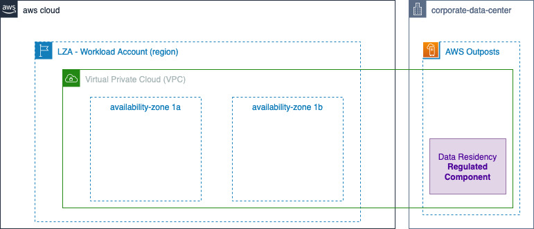
AWS Outposts is a fully managed service that brings the same AWS infrastructure, services, APIs, and tools to virtually any data center, colocation space, manufacturing floor, or on-premises facility where it might be needed. With Outposts, you can run some AWS services on-premises and connect to a broad range of services available in the local AWS Region. Outposts supports workloads requiring low latency, local data processing, data residency, and application migration.
Outposts capacity is driven as per your compute and storage requirements to run workloads. You can monitor Outposts resources using metrics gathered by Amazon CloudWatch. Using these metrics, you can effectively monitor and manage the Outposts resources as they would in the Region, levereging cloud native tools such as CloudWatch dashboards. Check the Monitoring best practices for AWS Outposts blog post to dive deep into the available monitoring options for Outposts.
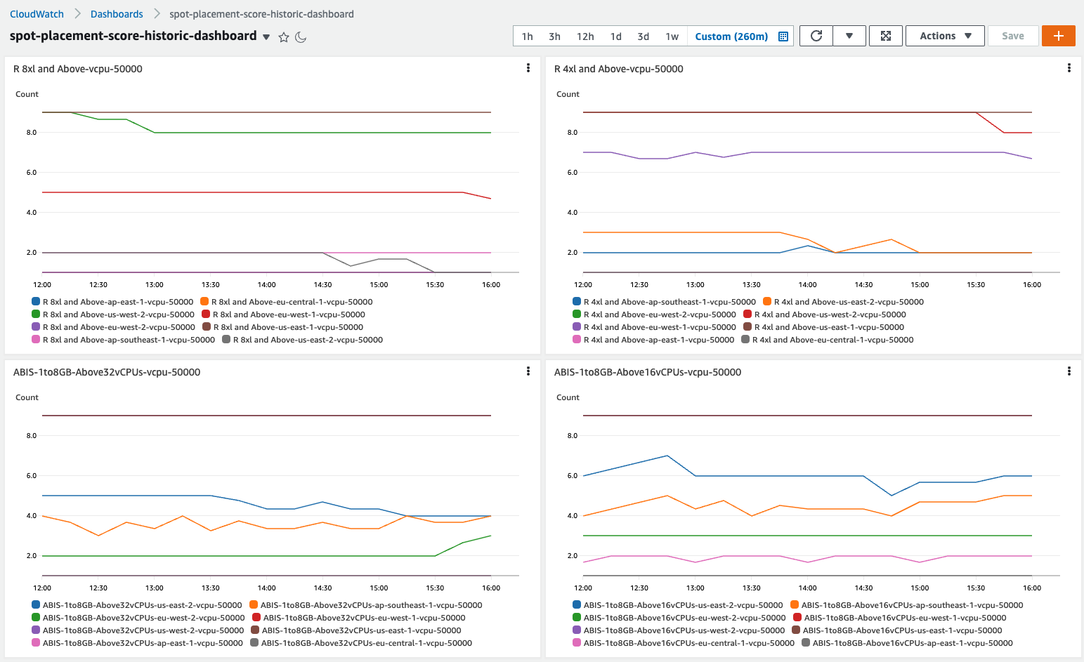
CloudWatch dashboards are customizable home pages in the CloudWatch console that can be used to monitor resources running on Outposts in a single view. For example, you can monitor in a single pane the number Amazon EC2 instances used per EC2 instance type, the available capacity of Amazon EBS volumes and Amazon S3 buckets, and the operational status of the service link of Outposts.
As a you start deploying additional Outposts resources as a part of their capacity expansion, they must all be integrated and visualized within CloudWatch in an automated way. Traditionally CloudWatch dashboards are built manually and may be time consuming to tune. This post provides also an overview of building CloudWatch dashboards in an automated way using AWS Cloud Development Kit (AWS CDK).
Overview
CloudWatch metrics available to monitor Outposts resources and capacity
CloudWatch metrics for Outposts are available to customers in all public AWS Regions and AWS GovCloud (US) at no additional cost. We can classify the available metrics in two main categories:
- Metrics that can be used to gain visibility into Outposts capacity and operativity, published mainly under AWS/Outposts namespace.For Amazon Simple Storage Service (Amazon S3) on Outpost, the capacity metrics are published under AWS/S3_Outposts namespace.
- Service specific metrics that can be used to monitor each resource hosted on Outposts, such as Amazon Elastic Compute Cloud (Amazon EC2), Amazon Elastic Load Balancer (Amazon ELB), Amazon Relational Database Service (Amazon RDS). Just like for any resource hosted in the Region, these metrics are published under service specific namespaces. For example, when you launch a new EC2 instance in Outposts, it starts publishing Amazon EC2 metrics under AWS/EC2
To identify the metrics published under the service specific namespaces, we can leverage metadata in the form of tags. A tag is a label that you assign to an AWS resource and consists of a key and an optional value. For the purpose of the monitoring strategy described in this post, we use a tag that contains the OutpostID of the Outpost where the resource is deployed. In this way, we can easily filter the CloudWatch metrics that we would like to show in our dashboard.
To enforce the assignment of tags to our resources we can implement a tagging strategy using AWS tag Policies and Service Control Policies (SCPs).
The following sections describe two different methods to build a CloudWatch dashboard that includes the different types of metrics described so far. In both cases, we see how particularly useful the presence of tags is to identify the service-specific metrics.
Manual approach to building a CloudWatch dashboard for Outposts
This section describes a manual (i.e., non-automated) approach to building a dashboard that could summarize both the capacity utilization metrics and the service specific metrics for your resources running on Outposts.
The benefit of this approach is that we can implement a fully operational dashboard directly from the CloudWatch console. However, it will simultaneously require more effort to properly tune the dashboard to satisfy your monitoring requirements.
You can start creating the dashboard opening the CloudWatch console and following the steps listed in the public documentation.
To display a metric under AWS/Outposts namespace we can choose any of the widgets available. Based on the nature of the data, we can choose different types of Widgets such as Number, Line, Gauge, Explorer, or you can even build your own custom widget.
Together with the Widget type, we must select Outposts namespace in the metric graph dialog box and then navigate to the specific metric of interest.
In case we are creating the dashboard in a different account than the Outposts owner, we must select the right account in the View data drop-down menu to see the Outposts metric in which we are interested.

After selecting one or more metrics we can select Create widget button.
For the service specific metrics, we recommend using the explorer widget. In this way, we can utilize the tagging strategy described earlier to automatically identify the metrics belonging to the resources running on Outposts. Check the documentation page for a step-by-step guide for creating an explorer widget based on tags.
Automated outpost dashboard
After we’ve seen how to build a dashboard manually from the console, in this secton we describe an automated approach to deploy a dashboard for Outposts through AWS CDK.
AWS CDK is an open source software development framework to model and provision your cloud application resources using familiar programming languages, including TypeScript, JavaScript, Python, C#, and Java. For the solution in this post, we use Python.
Architecture overview
The AWS CDK stack described in this post, assumes that the resources running on Outposts (EC2 instances, S3 buckets, Application Load Balancers (ALBs), and RDS instances) are tagged using the tagging strategy described earlier.
Specifying a tag name and a tag value in a configuration file automatically discovers the resources with that tag and adds the related metrics to the CloudWatch dashboard.
Together with the service specific metrics, it creates a series of widgets that we can use to monitor the capacity available and utilized in each Outpost that belongs to the account where the script is running.

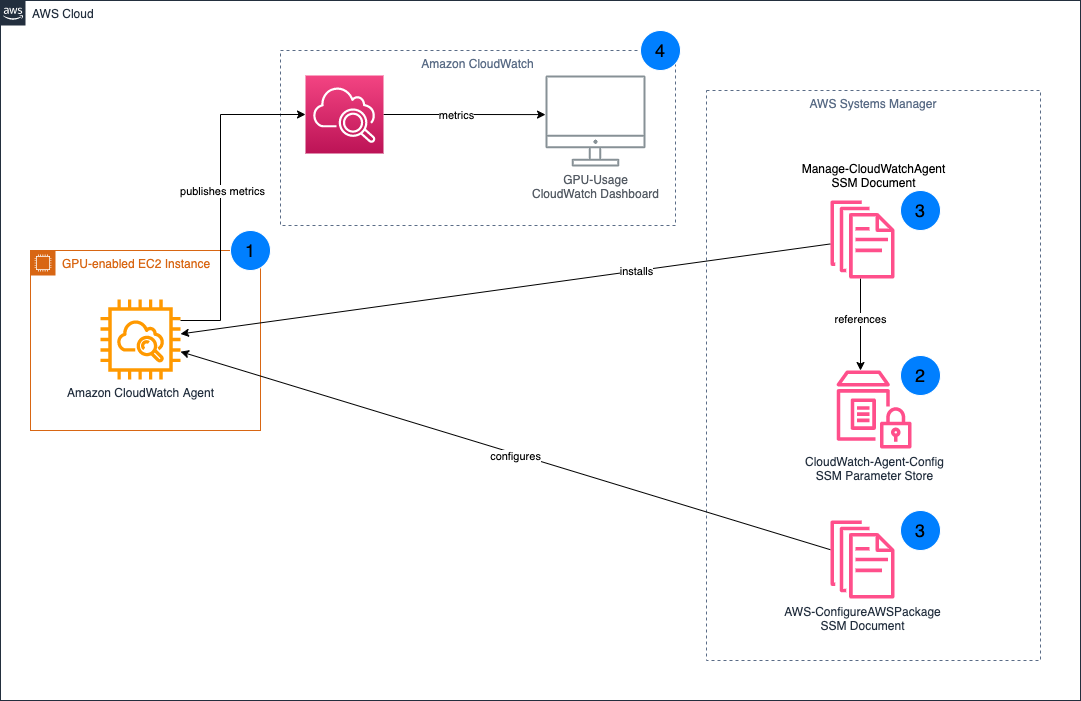
The workflow is made of the following phases:
- The AWS CDK stack creates an AWS CodeCommit repository and uploads its own code into it. The code contains a series of modules, one for each section of the CloudWatch dashboard. A section of the dashboard contains one or more widgets showing the metrics of a specific service.
- To maintain the CloudWatch dashboard always up-to-date with the resources matching the tag, it creates a pipeline in AWS CodePipeline that can dynamically create and or update the dashboard. The pipeline runs the code in the CodeCommit repository and is made of two stages. In the first one, the build stage, it builds the dependencies needed by the AWS CDK stack. In the second stage, the Deploy stage, it loads and runs the modules used to build the dashboard.
- Each module contains the code to automatically discover the tagged resources of a specific service. This discovery phase uses standard AWS APIs called through the Python SDK Boto3.
- Based on the results of the discovery phase, AWS CDK produces an AWS CloudFormation template containing the definition of the CloudWatch dashboard sections. The template is submitted to CloudFormation.
- CloudFormation creates or, if already defined, updates the CloudWatch dashboard.
- Together with the dashboard, the AWS CDK script also contains the definition of a CloudWatch Event that, once deployed, triggers the pipeline each time a resource tagged with the specified tag is created or destroyed.
Prerequisites
To implement the solution presented in this post, you must configure:
- git as distributed version control system.
- In case it is the first time that you’re using AWS CDK in this account and region, you must:
a. Install the AWS CDK, and its prerequisites, following these instructions.
b. Go through the AWS CDK bootstrapping process. This is required only for the first time that we use AWS CDK in a specific AWS environment (an AWS environment is a combination of an AWS account and Region).
How to install
Step 1: Clone the AWS CDK code hosted on GitHub with:
$ git clone https://github.com/aws-samples/automated-cloudwatch-dashboard.git
Step 2: enter the directory using the following:
$ cd automated-cloudwatch-dashboard/
Step 3: Install the needed Python dependencies with:
$ pip install -r requirements.txt
Step 4: Modify the configuration file
Before deploying the stack, we must modify the configuration file to specify the tag we use for identifying our resources running on Outposts. Open the file with the name config.yaml with your preferred text editor and specify:
-
-
- A name for the dashboard. The default name used is Automated-CloudWatch-Dashboard.
- Replace <tag_name> placeholder following the tag_name variable with the tag name used to tag the resources that you want to include in the dashboard.
- Replace <tag_value> placeholder under tag_values variable with the tag value that you used.
-
Here is an example config.yaml configuration file:
dashboard_name: Automated-CloudWatch-Dahsboard
tag_name: OutpostID
tag_values:
  - op-1234567890abcdefg
Stack deployment
We can deploy the stack with the following:
$ cdk deploy
At the end of the deployment process, the pipeline that creates the dashboard is provisioned. You can now go to your CloudWatch console to view it.
Automated Outposts dashboard overview
Now that we have built our dashboard, let’s review each section:
-
Outpost capacity

The AWS CDK stacks define a capacity section for each Outpost available to the AWS account where the script runs.
In this section, we find four widgets showing metrics published under the AWS/Outpost namespace. The first widget shows for each EC2 instance type available on the Outposts the number of instances utilized and available for that instance type. In the second row, we can visualize the available capacity for the Amazon EBS volumes and for the S3 buckets. The last widget shows the operational status of the service link of Outposts.
2. EC2 instances

In this section of the dashboard, we find the metrics showing the CPU, Network, and Disk Utilization for an EC2 instance. It has defined a section of this type for each EC2 instance with a tag assigned matching the name and the value specified in the configuration file of the script.
3. Application Load Balancer

The ALB section aggregates metrics showing the operational status of a load balancer hosted on Outposts. A section of this type is defined for each ALB with an assigned tag matching the one specified in the configuration file.
4. S3 buckets

The S3 buckets section is defined only once and aggregates the utilization metrics for all S3 buckets with an assigned tag.
5. AutoScaling group

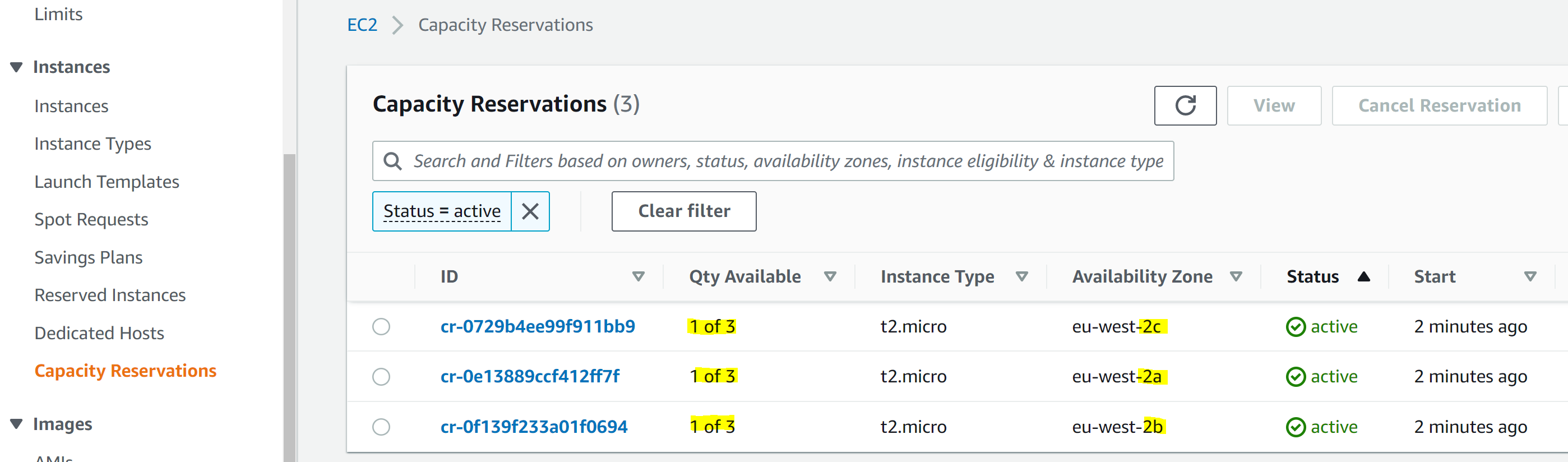
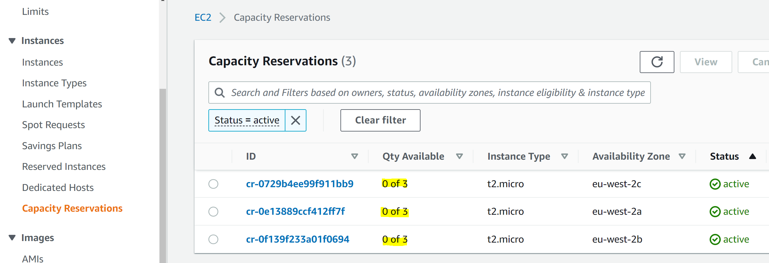
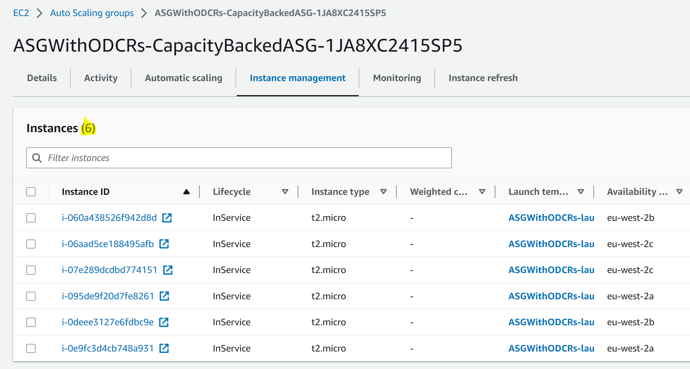
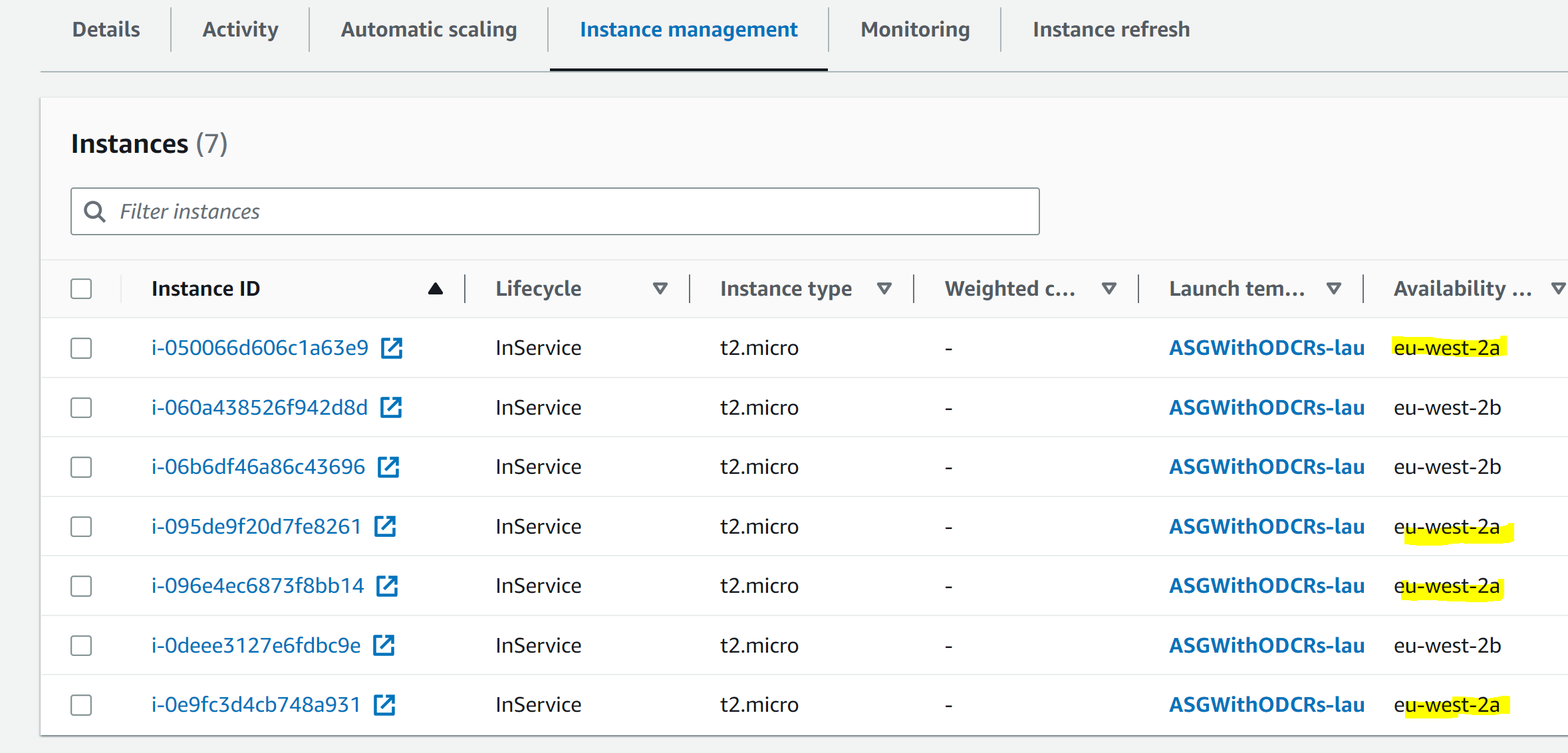
The AutoScaling group section can be used to monitor the number of instances in service in a specific AS group with a tag assigned. This section is defined once and can aggregate the metrics for multiple AutoScaling groups.
Clean up
To terminate the resources that we created in this post, run the following:
$ cdk destroy
Then, go to the Cloudformation console and delete the stack with the name “Deploy-AutomatedCloudWatchDashboard”.
Conclusion
In conclusion, this post demonstrates a manual way of creating CloudWatch Metrics dashboard using the CloudWatch console and an automated way using AWS CDK. The automated approach is also scalable by automatically discovering any new resources added to the existing Outposts in the your environment without any changes to the code.