At Hot Chips 2026, NVIDIA went into detail on its upcoming Vera server CPU, and the Olympus CPU architecture. With 88 cores per chip, NVIDIA has ambitious aims for its in-house designed CPU architecture
NVIDIA this morning has released a trove of new technical details on Vera, their upcoming server CPU, as well as the Olympus CPU core. The company is also publishing the first SPEC CPU 2026 benchmarks, giving us our best look yet at the performance of the chip
AMD is adding a trio of new chips to its Ryzen AI Max portfolio. The 400 series chips will bring support for up to 192GB of memory to AI systems, allowing for larger local models than ever before
AMD’s Ryzen 9000 series desktop processors are by now well into the second half of their lifecycle as AMD’s leading-edge desktop chips. With a complete product stack in play – ranging from 6 up to 16 CPU cores on a single chip – In most generations this would be where AMD would stand pat on […]
While NVIDIA is best known as a GPU company for obvious reasons, the company has now spent almost half of its existence trying to branch into the CPU market as well. From early forays into processor designs with Denver – and ambitions of x86 processors unrealized – through multiple generations of Tegra SoCs, and now […]
Amid a slew of telecom and commercial client announcements today designed to align with the opening of Mobile World Congress 2026, AMD is using the show as a backdrop to launch the desktop versions of their Ryzen AI 400 chips. First teased back during CES 2026, the company is finally giving them a proper launch […]
Imagine this — you click play on Netflix on a Friday night and behind the scenes hundreds of containers spring to action in a few seconds to answer your call. At Netflix, scaling containers efficiently is critical to delivering a seamless streaming experience to millions of members worldwide. To keep up with responsiveness at this scale, we modernized our container runtime, only to hit a surprising bottleneck: the CPU architecture itself.
Let us walk you through the story of how we diagnosed the problem and what we learned about scaling containers at the hardware level.
The Problem
When application demand requires that we scale up our servers, we get a new instance from AWS. To use this new capacity efficiently, pods are assigned to the node until its resources are considered fully allocated. A node can go from no applications running to being maxed out within moments of being ready to receive these applications.
As we migrated more and more from our old container platform to our new container platform, we started seeing some concerning trends. Some nodes were stalling for long periods of time, with a simple health check timing out after 30 seconds. An initial investigation showed that the mount table length was increasing dramatically in these situations, and reading it alone could take upwards of 30 seconds. Looking at systemd’s stack it was clear that it was busy processing these mount events as well and could lead to complete system lockup. Kubelet also timed out frequently talking to containerd in this period. Examining the mount table made it clear that these mounts were related to container creation.
The affected nodes were almost all r5.metal instances, and were starting applications whose container image contained many layers (50+).
Challenge
Mount Lock Contention
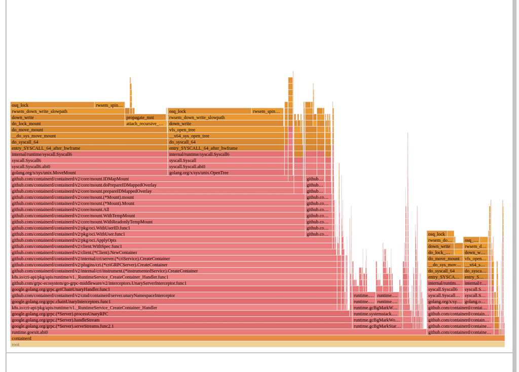
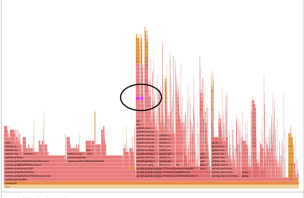
The flamegraph in Figure 1 clearly shows where containerd spent its time. Almost all of the time is spent trying to grab a kernel-level lock as part of the various mount-related activities when assembling the container’s root filesystem!
Figure 1: Flamegraph depicting lock contention
Looking closer, containerd executes the following calls for each layer if using user namespaces:
open_tree() to get a reference to the layer / directory
mount_setattr() to set the idmap to match the container’s user range, shifting the ownership so this container can access the files
move_mount() to create a bind mount on the host with this new idmap applied
These bind mounts are owned by the container’s user range and are then used as the lowerdirs to create the overlayfs-based rootfs for the container. Once the overlayfs rootfs is mounted, the bind mounts are then unmounted since they are not necessary to keep around once the overlayfs is constructed.
If a node is starting many containers at once, every CPU ends up busy trying to execute these mounts and umounts. The kernel VFS has various global locks related to the mount table, and each of these mounts requires taking that lock as we can see in the top of the flamegraph. Any system trying to quickly set up many containers is prone to this, and this is a function of the number of layers in the container image.
For example, assume a node is starting 100 containers, each with 50 layers in its image. Each container will need 50 bind mounts to do the idmap for each layer. The container’s overlayfs mount will be created using those bind mounts as the lower directories, and then all 50 bind mounts can be cleaned up via umount. Containerd actually goes through this process twice, once to determine some user information in the image and once to create the actual rootfs. This means the total number of mount operations on the start up path for our 100 containers is 100 * 2 * (1 + 50 + 50) = 20200 mounts, all of which require grabbing various global mount related locks!
Diagnosis
What’s Different In The New Runtime?
As alluded to in the introduction, Netflix has been undergoing a modernization of its container runtime. In the past a virtual kubelet + docker solution was used, whereas now a kubelet + containerd solution is being used. Both the old runtime and the new runtime used user namespaces, so what’s the difference here?
Old Runtime: All containers shared a single host user range. UIDs in image layers were shifted at untar time, so file permissions matched when containers accessed files. This worked because all containers used the same host user.
New Runtime: Each container gets a unique host user range, improving security — if a container escapes, it can only affect its own files. To avoid the costly process of untarring and shifting UIDs for every container, the new runtime uses the kernel’s idmap feature. This allows efficient UID mapping per container without copying or changing file ownership, which is why containerd performs many mounts.
Figure 2 below is a simplified example of how this idmap feature looks like:
Figure 2: idmap feature
Why Does Instance Type Matter?
As noted earlier, the issue was predominantly occurring on r5.metal instances. Once we identified the root issue we could easily reproduce by creating a container image with many layers and sending hundreds of workloads using the image to a test node.
To better understand why this bottleneck was more profound on some instances compared to others, we benchmarked container launches on different AWS instance types:
r5.metal (5th gen Intel, dual-socket, multiple NUMA domains)
m7i.metal-24xl (7th gen Intel, single-socket, single NUMA domain)
m7a.24xlarge (7th gen AMD, single-socket, single NUMA domain)
Baseline Results
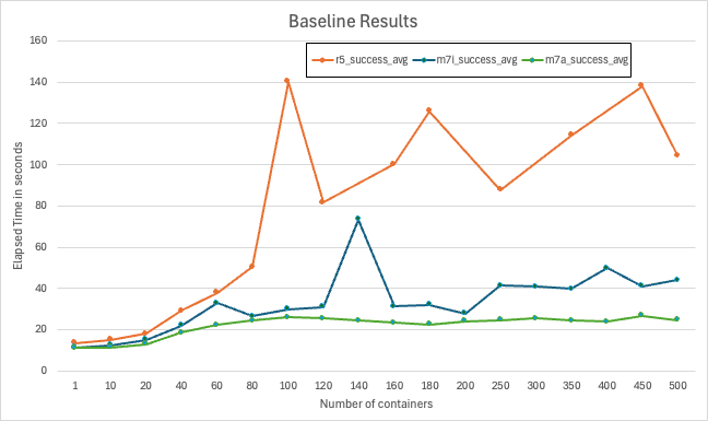
Figure 3 shows the baseline results from scaling containers on each instance type
At low concurrency (≤ ~20 containers), all platforms performed similarly
As concurrency increased, r5.metal began to fail around 100 containers
7th generation AWS instances maintained lower launch times and higher success rates as concurrency grew
m7a instances showed the most consistent scaling behavior with the lowest failure rates even at high concurrency
Deep Dive
Using perf record and custom microbenchmarks, we can see the hottest code path was in the Linux kernel’s Virtual Filesystem (VFS) path lookup code — specifically, a tight spin loop waiting on a sequence lock in path_init(). The CPU spent most of its time executing the pause instruction, indicating many threads were spinning, waiting for the global lock, as shown in the disassembly snippet below
path_init():
…
mov mount_lock,%eax
test $0x1,%al
je 7c
pause
…
Using Intel’s Topdown Microarchitecture Analysis (TMA), we observed:
95.5% of pipeline slots were stalled on contested accesses (tma_contested_accesses).
57% of slots were due to false sharing (multiple cores accessing the same cache line).
Cache line bouncing and lock contention were the primary culprits.
Given a high amount of time being spent in contested accesses, the natural thinking from a perspective of hardware variations led to investigation of NUMA and Hyperthreading impact coming from the architecture to this subset
NUMA Effects
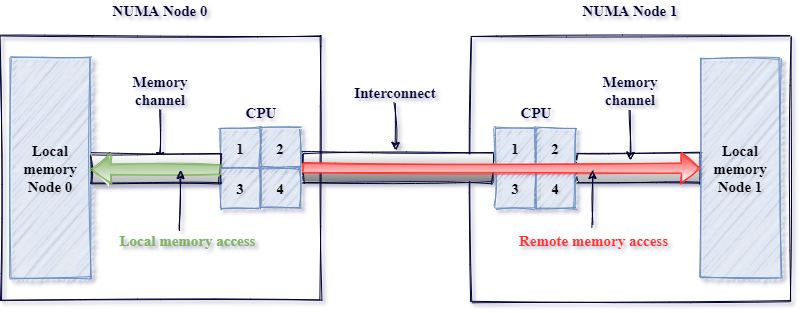
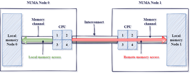
Non-Uniform Memory Access (NUMA) is a system design where each processor has its own local memory for faster access but relies on an interconnect to access the memory attached to a remote processor. Introduced in the 1990s to improve scalability in multiprocessor systems, NUMA boosts performance but also introduces higher latency when a CPU needs to access memory attached to another processor. Figure 4 is a simple image describing local vs remote access patterns of a NUMA architecture
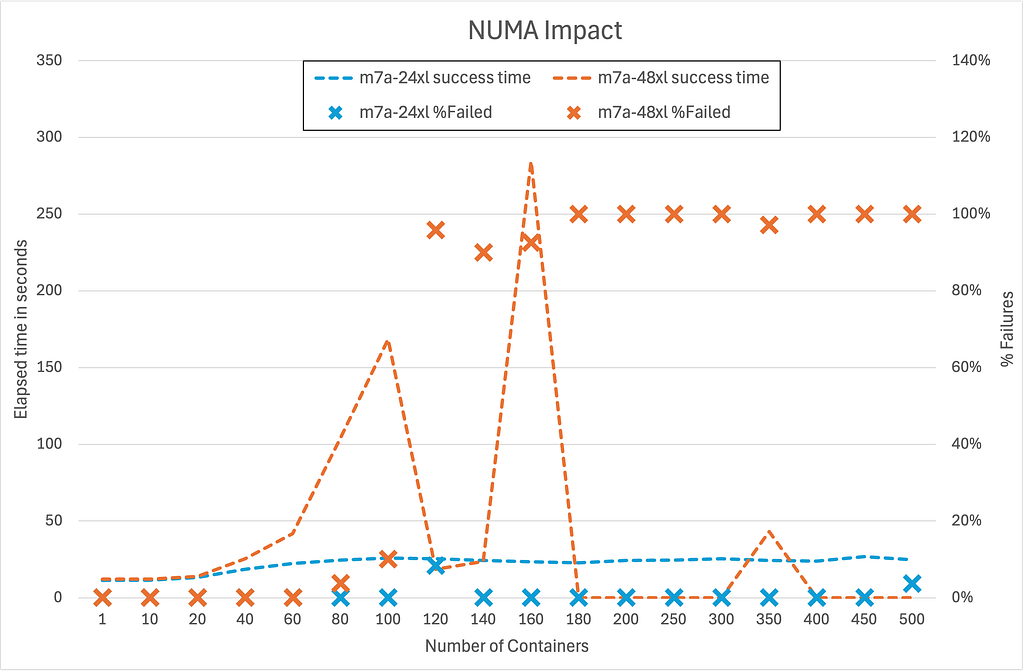
AWS instances come in a variety of shapes and sizes. To obtain the largest core count, we tested the 2-socket 5th generation metal instances (r5.metal), on which containers were orchestrated by the titus agent. Modern dual-socket architectures implement NUMA design, leading to faster local but higher remote access latencies. Although container orchestration can maintain locality, global locks can easily run into high latency effects due to remote synchronization. In order to test the impact of NUMA, we tested an AWS 48xl sized instance with 2 NUMA nodes or sockets versus an AWS 24xl sized instance, which represents a single NUMA node or socket. As seen from Figure 5, the extra hop introduces high latencies and hence failures very quickly.
Figure 5: Numa Impact
Hyperthreading Effects
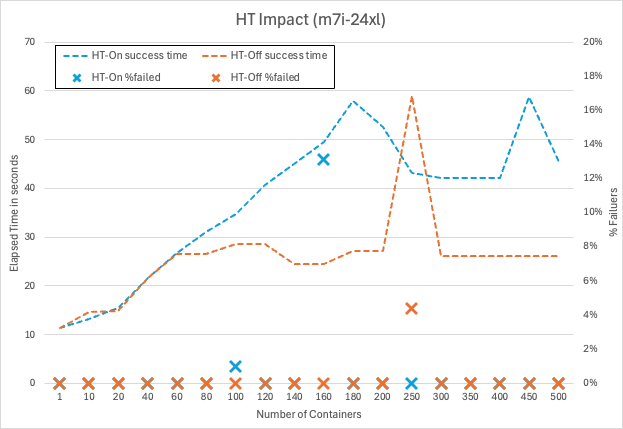
Hyperthreading (HT): Disabling HT on m7i.metal-24xl (Intel) improved container launch latencies by 20–30% as seen in Figure 6, since hyperthreads compete for shared execution resources, worsening the lock contention. When hyperthreading is enabled, each physical CPU core is split into two logical CPUs (hyperthreads) that share most of the core’s execution resources, such as caches, execution units, and memory bandwidth. While this can improve throughput for workloads that are not fully utilizing the core, it introduces significant challenges for workloads that rely heavily on global locks. By disabling hyperthreading, each thread runs on its own physical core, eliminating this competition for shared resources between hyperthreads. As a result, threads can acquire and release global locks more quickly, reducing overall contention and improving latency for operations that generally share underlying resources.
Figure 6: Hyperthreading impact
Why Does Hardware Architecture Matter?
Centralized Cache Architectures
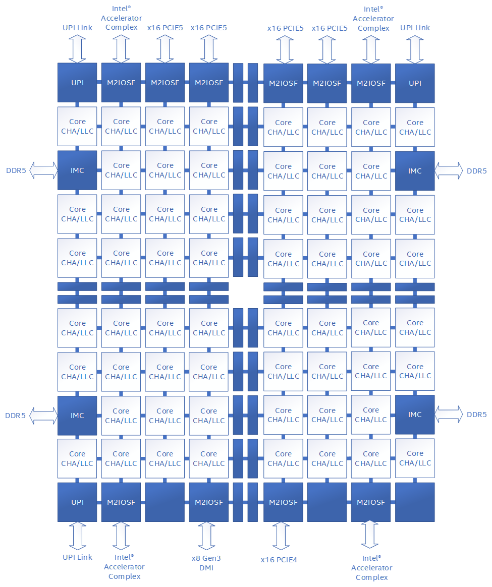
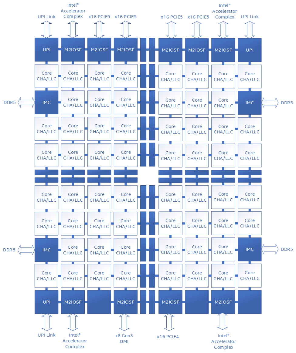
Some modern server CPUs use a mesh-style interconnect to link cores and cache slices, with each intersection managing cache coherence for a subset of memory addresses. In these designs, all communication passes through a central queueing structure, which can only handle one request for a given address at a time. When a global lock (like the mount lock) is under heavy contention, all atomic operations targeting that lock are funneled through this single queue, causing requests to pile up and resulting in memory stalls and latency spikes.
In some well-known mesh-based architectures as shown in Figure 7 below, this central queue is called the “Table of Requests” (TOR), and it can become a surprising bottleneck when many threads are fighting for the same lock. If you’ve ever wondered why certain CPUs seem to “pause for breath” under heavy contention, this is often the culprit.
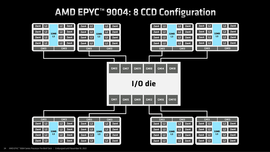
Some modern server CPUs use a distributed, chiplet-based architecture (Figure 8), where multiple core complexes, each with their own local last-level cache — are connected via a high-speed interconnect fabric. In these designs, cache coherence is managed within each core complex, and traffic between complexes is handled by a scalable control fabric. Unlike mesh-based architectures with centralized queueing structures, this distributed approach spreads contention across multiple domains, making severe stalls from global lock contention less likely. For those interested in the technical details, public documentation from major CPU vendors provides deeper insight into these distributed cache and chiplet designs.
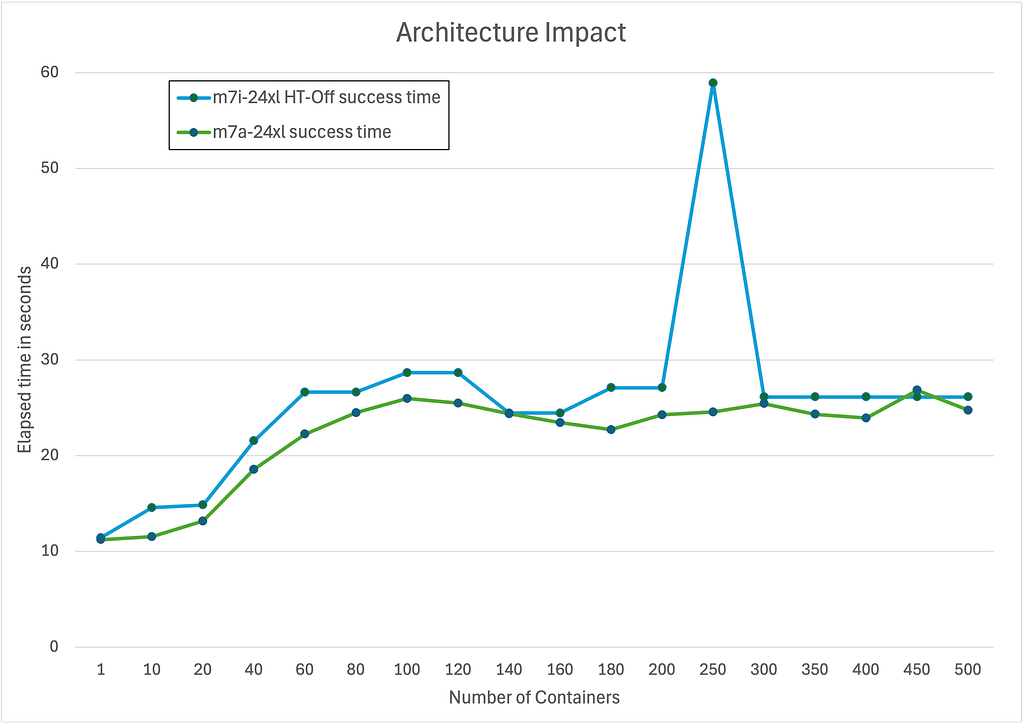
Here is a comparison of the same workload run on m7i (centralized cache architecture) vs m7a (distributed cache architecture). Note that, in order to make it closely comparable, Hyperthreading (HT) was disabled on m7i, given previous regression seen in Figure 6, and experiments were run using same core counts. The result clearly shows a fairly consistent difference in performance of approximately 20% as shown in Figure 9
Figure 9: Architectural impact between m7i and m7a
Microbenchmark Results
To prove the above theory related to NUMA, HT and micro-architecture, we developed a small microbenchmark which basically invokes a given number of threads that then spins on a globally contended lock. Running the benchmark at increasing thread counts reveals the latency characteristics of the system under different scenarios. For example, Figure 10 below is the microbenchmark results with NUMA, HT and different microarchitectures.
Figure 10: Global lock contention benchmark results
Results from this custom synthetic benchmark (pause_bench) confirmed:
On r5.metal, eliminating NUMA by only using a single socket significantly drops latency at high thread counts
On m7i.metal-24xl, disabling hyperthreading further improves scaling
On m7a.24xlarge, performance scales the best, demonstrating that a distributed cache architecture handles cache-line contention in this case of global locks more gracefully.
Improving Software Architecture
While understanding the impacts of the hardware architecture is important for assessing possible mitigations, the root cause here is contention over a global lock. Working with containerd upstream we came to two possible solutions:
Use the newer kernel mount API’s fsconfig() lowerdir+ support to supply the idmap’ed lowerdirs as fd’s instead of filesystem paths. This avoids the move_mount() syscall mentioned prior which requires global locks to mount each layer to the mount table
Map the common parent directory of all the layers. This makes the number of mount operations go from O(n) to O(1) per container, where n is the number of layers in the image
Since using the newer API requires using a new kernel, we opted to make the latter change to benefit more of the community. With that in place, no longer do we see containerd’s flamegraph being dominated by mount-related operations. In fact, as seen in Figure 11 below we had to highlight them in purple below to see them at all!
Figure 11: Optimized solution
Conclusion
Our journey migrating to a modern kubelet + containerd runtime at Netflix revealed just how deeply intertwined software and hardware architecture can be when operating at scale. While kubelet/containerd’s usage of unique container users brought significant security gains, it also surfaced new bottlenecks rooted in kernel and CPU architecture — particularly when launching hundreds of many layered container images in parallel. Our investigation highlighted that not all hardware is created equal for this workload: centralized cache management amplified cache contention while distributed cache design smoothly scaled under load.
Ultimately, the best solution combined hardware awareness with software improvements. For an immediate mitigation we chose to route these workloads to CPU architectures that scaled better under these conditions. By changing the software design to minimize per-layer mount operations, we eliminated the global lock as a launch-time bottleneck — unlocking faster, more reliable scaling regardless of the underlying CPU architecture. This experience underscores the importance of holistic performance engineering: understanding and optimizing both the software stack and the hardware it runs on is key to delivering seamless user experiences at Netflix scale.
We trust these insights will assist others in navigating the evolving container ecosystem, transforming potential challenges into opportunities for building robust, high-performance platforms.
Special thanks to the Titus and Performance Engineering teams at Netflix.
Alongside AMD’s numerous client-focused hardware announcements during their CES 2026 keynote, the company also devoted a bit of attention to their data center/server products. Though the company is essentially mid-cycle on its major data center products right now – and thus is not launching anything in the immediate timeframe – AMD still opted to use […]
Alongside AMD’s slew of consumer-related product announcements with desktop and mobile Ryzen processors, the company also took a moment of its time during its CES 2026 presentation to address the embedded market. The tangentially-related cousin to the consumer market, AMD’s embedded lineup of processors are aimed at the automotive and industrial markets, as well as […]
Kicking off AMD’s slate of consumer announcements for this year’s CES trade show, the company brought to the shows several new chip SKUs for the consumer market. Altogether the company is launching two new Ryzen AI Max+ processors for AI developers, a new desktop Ryzen 9000X3D chip for gamers, and for the mobile market a […]
Closing out their hour-long, AI-focused Computex keynote, Qualcomm CEO Cristiano Amon ended his presentation with a brief teaser of what’s in store for the server side of Qualcomm’s hardware business. The company has repeatedly dabbled in the server market with products such as their Cloud AI 100 inference accelerators. But thus far Qualcomm has not […]
At Netflix, the Analytics and Developer Experience organization, part of the Data Platform, offers a product called Workbench. Workbench is a remote development workspace based on Titus that allows data practitioners to work with big data and machine learning use cases at scale. A common use case for Workbench is running JupyterLab Notebooks.
Recently, several users reported that their JupyterLab UI becomes slow and unresponsive when running certain notebooks. This document details the intriguing process of debugging this issue, all the way from the UI down to the Linux kernel.
Symptom
Machine Learning engineer Luca Pozzi reported to our Data Platform team that their JupyterLab UI on their workbench becomes slow and unresponsive when running some of their Notebooks. Restarting the ipykernel process, which runs the Notebook, might temporarily alleviate the problem, but the frustration persists as more notebooks are run.
Quantify the Slowness
While we observed the issue firsthand, the term “UI being slow” is subjective and difficult to measure. To investigate this issue, we needed a quantitative analysis of the slowness.
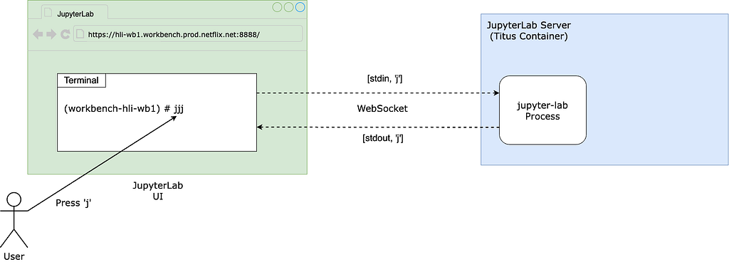
Itay Dafna devised an effective and simple method to quantify the UI slowness. Specifically, we opened a terminal via JupyterLab and held down a key (e.g., “j”) for 15 seconds while running the user’s notebook. The input to stdin is sent to the backend (i.e., JupyterLab) via a WebSocket, and the output to stdout is sent back from the backend and displayed on the UI. We then exported the .har file recording all communications from the browser and loaded it into a Notebook for analysis.
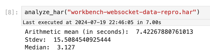
Using this approach, we observed latencies ranging from 1 to 10 seconds, averaging 7.4 seconds.
Blame The Notebook
Now that we have an objective metric for the slowness, let’s officially start our investigation. If you have read the symptom carefully, you must have noticed that the slowness only occurs when the user runs certain notebooks but not others.
Therefore, the first step is scrutinizing the specific Notebook experiencing the issue. Why does the UI always slow down after running this particular Notebook? Naturally, you would think that there must be something wrong with the code running in it.
Upon closely examining the user’s Notebook, we noticed a library called pystan , which provides Python bindings to a native C++ library called stan, looked suspicious. Specifically, pystan uses asyncio. However, because there is already an existing asyncio event loop running in the Notebook process and asyncio cannot be nested by design, in order for pystan to work, the authors of pystanrecommend injecting pystan into the existing event loop by using a package called nest_asyncio, a library that became unmaintained because the author unfortunately passed away.
Given this seemingly hacky usage, we naturally suspected that the events injected by pystan into the event loop were blocking the handling of the WebSocket messages used to communicate with the JupyterLab UI. This reasoning sounds very plausible. However, the user claimed that there were cases when a Notebook not using pystan runs, the UI also became slow.
Moreover, after several rounds of discussion with ChatGPT, we learned more about the architecture and realized that, in theory, the usage of pystan and nest_asyncio should not cause the slowness in handling the UI WebSocket for the following reasons:
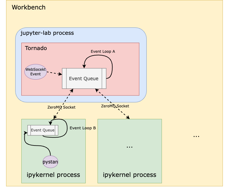
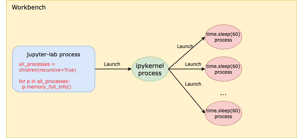
Even though pystan uses nest_asyncio to inject itself into the main event loop, the Notebook runs on a child process (i.e., the ipykernel process) of the jupyter-lab server process, which means the main event loop being injected by pystan is that of the ipykernel process, not the jupyter-server process. Therefore, even if pystan blocks the event loop, it shouldn’t impact the jupyter-lab main event loop that is used for UI websocket communication. See the diagram below:
In other words, pystan events are injected to the event loop B in this diagram instead of event loop A. So, it shouldn’t block the UI WebSocket events.
You might also think that because event loop A handles both the WebSocket events from the UI and the ZeroMQ socket events from the ipykernel process, a high volume of ZeroMQ events generated by the notebook could block the WebSocket. However, when we captured packets on the ZeroMQ socket while reproducing the issue, we didn’t observe heavy traffic on this socket that could cause such blocking.
A stronger piece of evidence to rule out pystan was that we were ultimately able to reproduce the issue even without it, which I’ll dive into later.
Blame Noisy Neighbors
The Workbench instance runs as a Titus container. To efficiently utilize our compute resources, Titus employs a CPU oversubscription feature, meaning the combined virtual CPUs allocated to containers exceed the number of available physical CPUs on a Titus agent. If a container is unfortunate enough to be scheduled alongside other “noisy” containers — those that consume a lot of CPU resources — it could suffer from CPU deficiency.
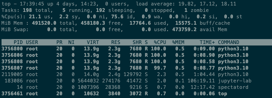
However, after examining the CPU utilization of neighboring containers on the same Titus agent as the Workbench instance, as well as the overall CPU utilization of the Titus agent, we quickly ruled out this hypothesis. Using the top command on the Workbench, we observed that when running the Notebook, the Workbench instance uses only 4 out of the 64 CPUs allocated to it. Simply put, this workload is not CPU-bound.
Blame The Network
The next theory was that the network between the web browser UI (on the laptop) and the JupyterLab server was slow. To investigate, we captured all the packets between the laptop and the server while running the Notebook and continuously pressing ‘j’ in the terminal.
When the UI experienced delays, we observed a 5-second pause in packet transmission from server port 8888 to the laptop. Meanwhile, traffic from other ports, such as port 22 for SSH, remained unaffected. This led us to conclude that the pause was caused by the application running on port 8888 (i.e., the JupyterLab process) rather than the network.
The Minimal Reproduction
As previously mentioned, another strong piece of evidence proving the innocence of pystan was that we could reproduce the issue without it. By gradually stripping down the “bad” Notebook, we eventually arrived at a minimal snippet of code that reproduces the issue without any third-party dependencies or complex logic:
import time
import os
from multiprocessing import Process

N = os.cpu_count()

def launch_worker(worker_id):
  time.sleep(60)

if __name__ == '__main__':
  with open('/root/2GB_file', 'r') as file:
    data = file.read()
    processes = []
    for i in range(N):
      p = Process(target=launch_worker, args=(i,))
      processes.append(p)
      p.start()

    for p in processes:
      p.join()
The code does only two things:
Read a 2GB file into memory (the Workbench instance has 480G memory in total so this memory usage is almost negligible).
Start N processes where N is the number of CPUs. The N processes do nothing but sleep.
There is no doubt that this is the most silly piece of code I’ve ever written. It is neither CPU bound nor memory bound. Yet it can cause the JupyterLab UI to stall for as many as 10 seconds!
Questions
There are a couple of interesting observations that raise several questions:
We noticed that both steps are required in order to reproduce the issue. If you don’t read the 2GB file (that is not even used!), the issue is not reproducible. Why using 2GB out of 480GB memory could impact the performance?
When the UI delay occurs, the jupyter-lab process CPU utilization spikes to 100%, hinting at contention on the single-threaded event loop in this process (event loop A in the diagram before). What does the jupyter-lab process need the CPU for, given that it is not the process that runs the Notebook?
The code runs in a Notebook, which means it runs in the ipykernel process, that is a child process of the jupyter-lab process. How can anything that happens in a child process cause the parent process to have CPU contention?
The workbench has 64CPUs. But when we printed os.cpu_count(), the output was 96. That means the code starts more processes than the number of CPUs. Why is that?
Let’s answer the last question first. In fact, if you run lscpu and nproc commands inside a Titus container, you will also see different results — the former gives you 96, which is the number of physical CPUs on the Titus agent, whereas the latter gives you 64, which is the number of virtual CPUs allocated to the container. This discrepancy is due to the lack of a “CPU namespace” in the Linux kernel, causing the number of physical CPUs to be leaked to the container when calling certain functions to get the CPU count. The assumption here is that Python os.cpu_count() uses the same function as the lscpu command, causing it to get the CPU count of the host instead of the container. Python 3.13 has a new call that can be used to get the accurate CPU count, but it’s not GA’ed yet.
It will be proven later that this inaccurate number of CPUs can be a contributing factor to the slowness.
More Clues
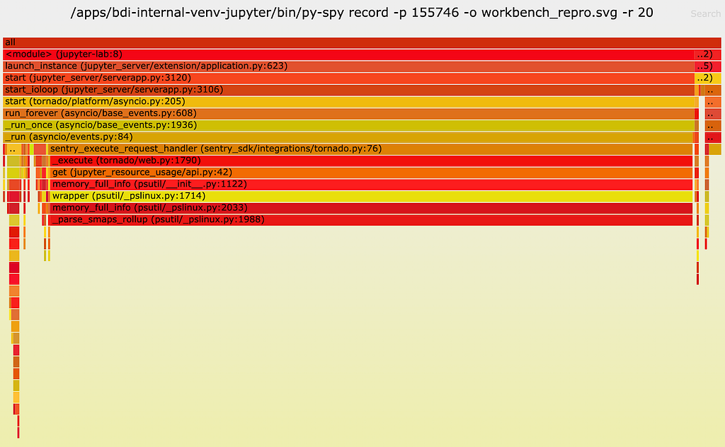
Next, we used py-spy to do a profiling of the jupyter-lab process. Note that we profiled the parent jupyter-lab process, not the ipykernel child process that runs the reproduction code. The profiling result is as follows:
As one can see, a lot of CPU time (89%!!) is spent on a function called __parse_smaps_rollup. In comparison, the terminal handler used only 0.47% CPU time. From the stack trace, we see that this function is inside the event loop A, so it can definitely cause the UI WebSocket events to be delayed.
The stack trace also shows that this function is ultimately called by a function used by a Jupyter lab extension called jupyter_resource_usage. We then disabled this extension and restarted the jupyter-lab process. As you may have guessed, we could no longer reproduce the slowness!
But our puzzle is not solved yet. Why does this extension cause the UI to slow down? Let’s keep digging.
Root Cause Analysis
From the name of the extension and the names of the other functions it calls, we can infer that this extension is used to get resources such as CPU and memory usage information. Examining the code, we see that this function call stack is triggered when an API endpoint /metrics/v1 is called from the UI. The UI apparently calls this function periodically, according to the network traffic tab in Chrome’s Developer Tools.
Now let’s look at the implementation starting from the call get(jupter_resource_usage/api.py:42) . The full code is here and the key lines are shown below:
for p in all_processes: info = p.memory_full_info()
Basically, it gets all children processes of the jupyter-lab process recursively, including both the ipykernel Notebook process and all processes created by the Notebook. Obviously, the cost of this function is linear to the number of all children processes. In the reproduction code, we create 96 processes. So here we will have at least 96 (sleep processes) + 1 (ipykernel process) + 1 (jupyter-lab process) = 98 processes when it should actually be 64 (allocated CPUs) + 1 (ipykernel process) + 1 (jupyter-lab process) = 66 processes, because the number of CPUs allocated to the container is, in fact, 64.
This is truly ironic. The more CPUs we have, the slower we are!
At this point, we have answered one question: Why does starting many grandchildren processes in the child process cause the parent process to be slow? Because the parent process runs a function that’s linear to the number all children process recursively.
However, this solves only half of the puzzle. If you remember the previous analysis, starting many child processes ALONE doesn’t reproduce the issue. If we don’t read the 2GB file, even if we create 2x more processes, we can’t reproduce the slowness.
So now we must answer the next question: Why does reading a 2GB file in the child process affect the parent process performance, especially when the workbench has as much as 480GB memory in total?
To answer this question, let’s look closely at the function __parse_smaps_rollup. As the name implies, this function parses the file /proc/<pid>/smaps_rollup.
def _parse_smaps_rollup(self):
  uss = pss = swap = 0
  with open_binary("{}/{}/smaps_rollup".format(self._procfs_path, self.pid)) as f:
  for line in f:
    if line.startswith(b”Private_”):
    # Private_Clean, Private_Dirty, Private_Hugetlb
      s uss += int(line.split()[1]) * 1024
    elif line.startswith(b”Pss:”):
      pss = int(line.split()[1]) * 1024
    elif line.startswith(b”Swap:”):
      swap = int(line.split()[1]) * 1024
return (uss, pss, swap)
Naturally, you might think that when memory usage increases, this file becomes larger in size, causing the function to take longer to parse. Unfortunately, this is not the answer because:
Second, this is a special file in the /proc filesystem, which should be seen as a kernel interface instead of a regular file on disk. In other words, I/O operations of this file are handled by the kernel rather than disk.
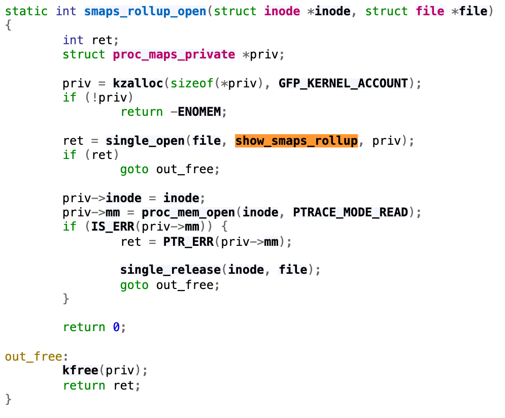
This file was introduced in this commit in 2017, with the purpose of improving the performance of user programs that determine aggregate memory statistics. Let’s first focus on the handler of open syscall on this /proc/<pid>/smaps_rollup.
Following through the single_openfunction, we will find that it uses the function show_smaps_rollup for the show operation, which can translate to the read system call on the file. Next, we look at the show_smaps_rollupimplementation. You will notice a do-while loop that is linear to the virtual memory area.
This perfectly explains why the function gets slower when a 2GB file is read into memory. Because the handler of reading the smaps_rollup file now takes longer to run the while loop. Basically, even though smaps_rollup already improved the performance of getting memory information compared to the old method of parsing the /proc/<pid>/smaps file, it is still linear to the virtual memory used.
More Quantitative Analysis
Even though at this point the puzzle is solved, let’s conduct a more quantitative analysis. How much is the time difference when reading the smaps_rollup file with small versus large virtual memory utilization? Let’s write some simple benchmark code like below:
import os

def read_smaps_rollup(pid):
  with open("/proc/{}/smaps_rollup".format(pid), "rb") as f:
    for line in f:
      pass

if __name__ == “__main__”:
  pid = os.getpid()

  read_smaps_rollup(pid)

  with open(“/root/2G_file”, “rb”) as f:
    data = f.read()

  read_smaps_rollup(pid)
This program performs the following steps:
Reads the smaps_rollup file of the current process.
Reads a 2GB file into memory.
Repeats step 1.
We then use strace to find the accurate time of reading the smaps_rollup file.
As you can see, both times, the read syscall returned 670, meaning the file size remained the same at 670 bytes. However, the time it took the second time (i.e., 0.027698 seconds) is 100x the time it took the first time (i.e., 0.000259 seconds)! This means that if there are 98 processes, the time spent on reading this file alone will be 98 * 0.027698 = 2.7 seconds! Such a delay can significantly affect the UI experience.
Solution
This extension is used to display the CPU and memory usage of the notebook process on the bar at the bottom of the Notebook:
We confirmed with the user that disabling the jupyter-resource-usage extension meets their requirements for UI responsiveness, and that this extension is not critical to their use case. Therefore, we provided a way for them to disable the extension.
Summary
This was such a challenging issue that required debugging from the UI all the way down to the Linux kernel. It is fascinating that the problem is linear to both the number of CPUs and the virtual memory size — two dimensions that are generally viewed separately.
Overall, we hope you enjoyed the irony of:
The extension used to monitor CPU usage causing CPU contention.
An interesting case where the more CPUs you have, the slower you get!
If you’re excited by tackling such technical challenges and have the opportunity to solve complex technical challenges and drive innovation, consider joining our Data Platform teams. Be part of shaping the future of Data Security and Infrastructure, Data Developer Experience, Analytics Infrastructure and Enablement, and more. Explore the impact you can make with us!
Is Raspberry Pi 4 a goodbye or a good buy for running Zabbix? How is it performance-wise? Is it reliable? Here’s my nine-month review of it, with a splash of appliance/application performance monitoring.
In about April 2022 when it became clear that I am going to continue my home monitoring project, I bought a Raspberry Pi 4 to run the show. Here’s my opinion on how well it is suited for running Zabbix.
Installing Zabbix
Applying that delicious layer of Zabbix on top of your Raspberry Pi 4 cake is extremely straightforward, as just like for every other platform that Zabbix officially supports, they do have packages and instructions to set up what you’d like to run.
So many options to choose from!
After installing the packages, the next steps are just like with Zabbix running on any other platform, so I am not going to dive into that now.
Modifications to my Raspberry setup
As I do not need to run a graphical environment on my Raspberry, I did disable the graphical environment from starting at all to save some precious RAM and other resources.
After some time I did also purchase an external USB hard disk, as the memory card from where Raspberry Pi 4 runs its OS is not very snappy, especially with write operations, and can also run tight on free space.
Other than that, my Raspberry Pi 4 is running pretty much by default.
How about the performance?
The graphs that you are about to see are from nine months period of time, as that’s about as long I have had the device.
No problem with the CPU usage. It’s been creeping up a little bit over time though, as I have been adding new items to monitoring and also additional software, such as HomeBridge and Home Assistant.
It still has available memory, even though the device runs Zabbix server, MariaDB, Grafana, Mosquitto, Home Assistant and HomeBridge.
As you can see, the number of running processes has grown significantly as I have been adding other stuff than Zabbix.
It’s easy to see when I did switch from an internal memory card to an external USB drive. The disk I/O utilization percentage is hovering at very tolerable levels.
I/O latency has remained about the same.
With only Zabbix, MariaDB and Grafana running the device remained around the 55-60C area, but has been warming to about 70C with the additional software. Still not too bad.
Splash of APM
Have you ever wondered what happens to the memory usage of a wrapper shell script that runs other scripts in a loop and keeps doing that until it’s manually stopped? This happens, it’s boringly stable. The results are brought you to by Zabbix Agent 2 process discovery.
Really, it does not vary much.
But as I have been adding new stuff, clearly the OS needs to do some more swapping and even the script has more page faults than before.
There’s more than that to process discovery, but those were some examples.
Zabbix server itself is doing very well, here are some example stats.
My conclusion: Raspberry Pi 4 is an excellent Zabbix server for smaller environments and a very good Zabbix proxy candidate. It’s been rock solid.
This post was originally published on the author’s page.
Cloudflare has millions of free customers. Not only is it something we’re incredibly proud of in the context of helping to build a better Internet — but it’s something that has made the Cloudflare service measurably better. One of the ways we’ve benefited is that it’s created a very strong imperative for Cloudflare to maintain a network that is as efficient as possible. There’s simply no other way to serve so many free customers.
In the spirit of this, we are very excited about the latest step in our energy-efficiency journey: turning to Arm for our server CPUs. It has been a long journey getting here — we started testing our first Arm CPUs all the way back in November 2017. It’s only recently, however, that the quantum of energy efficiency improvement from Arm has become clear. Our first Arm CPU was deployed in production earlier this month — July 2021.
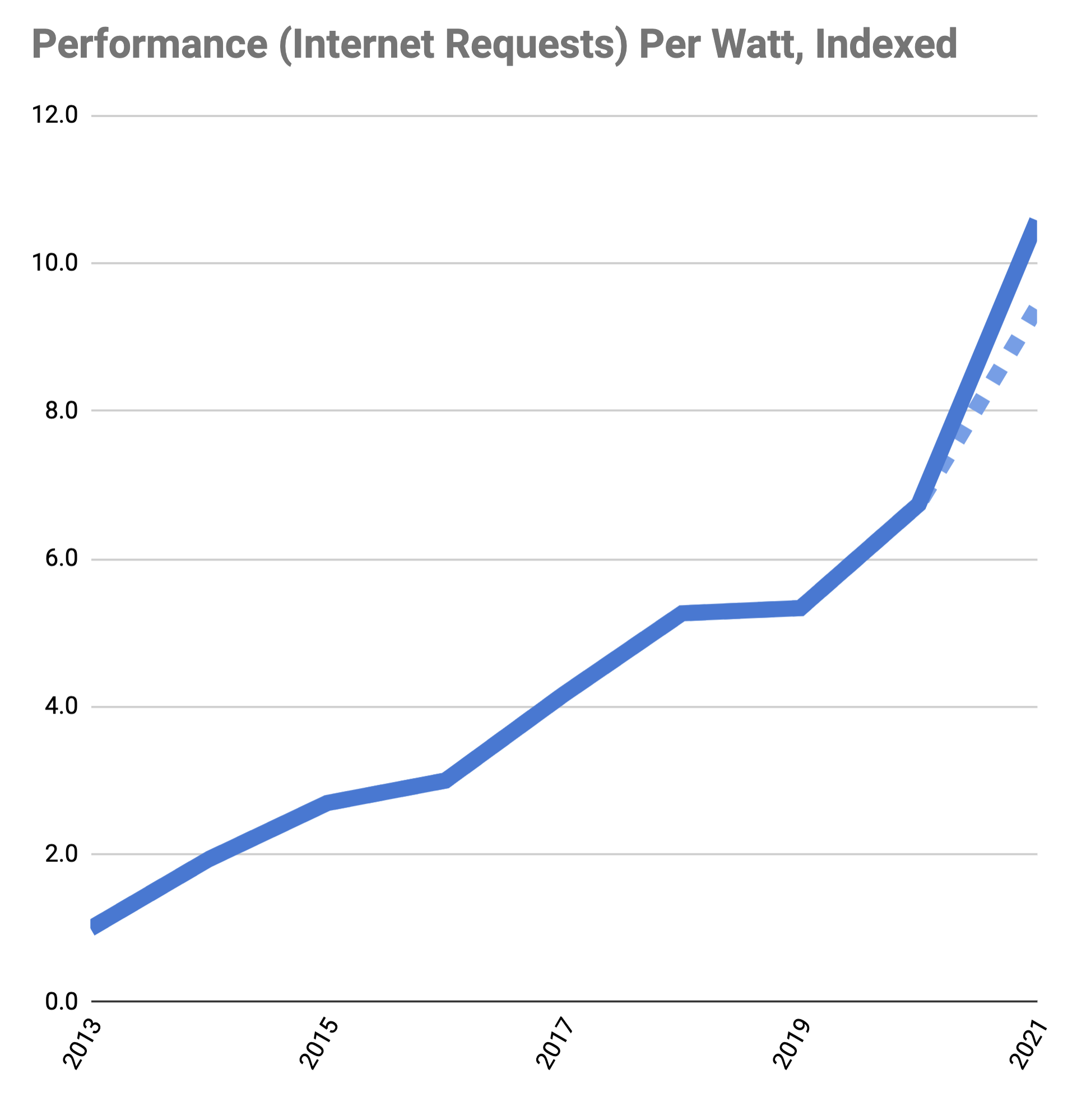
Our most recently deployed generation of edge servers, Gen X, used AMD Rome CPUs. Compared with that, the newest Arm based CPUs process an incredible 57% more Internet requests per watt. While AMD has a sequel, Milan (and which Cloudflare will also be deploying), it doesn’t achieve the same degree of energy efficiency that the Arm processor does — managing only 39% more requests per watt than Rome CPUs in our existing fleet. As Arm based CPUs become more widely deployed, and our software is further optimized to take advantage of the Arm architecture, we expect further improvements in the energy efficiency of Arm servers.
Using Arm, Cloudflare can now securely process over ten times as many Internet requests for every watt of power consumed, than we did for servers designed in 2013.
(In the graphic below, for 2021, the perforated data point refers to x86 CPUs, whereas the bold data point refers to Arm CPUs)
As Arm server CPUs demonstrate their performance and become more widely deployed, we hope this will inspire x86 CPUs manufacturers (such as Intel and AMD) to urgently take energy efficiency more seriously. This is especially important since, worldwide, x86 CPUs continue to represent the vast majority of global data center energy consumption.
Together, we can reduce the carbon impact of Internet use. The environment depends on it.
The collective thoughts of the interwebz
Manage Consent
To provide the best experiences, we use technologies like cookies to store and/or access device information. Consenting to these technologies will allow us to process data such as browsing behavior or unique IDs on this site. Not consenting or withdrawing consent, may adversely affect certain features and functions.
Functional
Always active
The technical storage or access is strictly necessary for the legitimate purpose of enabling the use of a specific service explicitly requested by the subscriber or user, or for the sole purpose of carrying out the transmission of a communication over an electronic communications network.
Preferences
The technical storage or access is necessary for the legitimate purpose of storing preferences that are not requested by the subscriber or user.
Statistics
The technical storage or access that is used exclusively for statistical purposes.The technical storage or access that is used exclusively for anonymous statistical purposes. Without a subpoena, voluntary compliance on the part of your Internet Service Provider, or additional records from a third party, information stored or retrieved for this purpose alone cannot usually be used to identify you.
Marketing
The technical storage or access is required to create user profiles to send advertising, or to track the user on a website or across several websites for similar marketing purposes.