Post Syndicated from Bhuvan Jain original https://aws.amazon.com/blogs/devops/automate-root-cause-analysis-across-datadog-and-elasticsearch-with-aws-devops-agent/
Modern distributed systems route business transactions through dozens of microservices, message queues, and event streams. When a message fails to process or processing exceeds SLA thresholds, troubleshooting requires correlating logs from tools like Elasticsearch, metrics from Datadog, and infrastructure change events in AWS CloudTrail. Correlating these signals manually across heterogeneous backends, each with different query languages, schemas, and time granularities, can take hours per incident and demands deep institutional knowledge of the system topology.
This post shows how AWS DevOps Agent, combined with a custom Model Context Protocol (MCP) server for Elasticsearch and native Datadog integration, automates end-to-end root cause analysis. When a Datadog alert fires, AWS DevOps Agent automatically initiates an investigation, correlates signals across all observability backends, and delivers root cause findings in minutes, without manual intervention.
In this post, we walk through the architecture, configuration steps, and a real-world scenario demonstrating how AWS DevOps Agent dramatically reduces mean time to identify (MTTI) for distributed system failures. DevOps engineers, site reliability engineers (SREs), and operations leaders managing containerized workloads will learn how to implement alert-triggered automated investigations that eliminate manual correlation and accelerate root cause identification in their own environments.
Challenges in correlating telemetry signals at scale
At scale, correlating telemetry signals across distributed systems is a key challenge. A platform processing billions of communications for regulated industries must track every message through its full lifecycle — ingestion, transformation, policy evaluation, archival, and retrieval — across dozens of production clusters, thousands of worker nodes, and terabytes of daily telemetry spread across multiple observability backends. A single message ID can generate log entries across multiple indices, correlated metrics in monitoring systems, and change events in audit trails. When a message goes missing or processing stalls, the operations team must pinpoint which cluster processed it, which log store holds the evidence, whether a recent deployment preceded the failure, and whether the issue is isolated or systemic — all while context-switching across tools with different query languages and data schemas. Before AWS DevOps Agent, this process routinely took hours per incident, and longer for complex multi-service failures.
The core difficulty is not the volume of data. It is the correlation of signals across heterogeneous systems that use different identifiers, different time granularities, and different data schemas. A message ID in Elasticsearch logs must be correlated to:
- A trace ID in application performance monitoring (APM) systems
- A pod name and namespace in Kubernetes event logs
- A container image tag in Amazon Elastic Container Registry (ECR) push events
- Metric anomalies (error rate spikes, pod restarts, CPU/memory deviations) in Datadog
- Deployment events captured in AWS CloudTrail logs
Manual correlation requires engineers to maintain mental models of these relationships while executing queries across multiple systems. It is error-prone, non-repeatable, and heavily dependent on institutional knowledge. When the engineer with the deepest system familiarity is unavailable, resolution times increases.
Prerequisites
Complete the following prerequisites before configuring the integrations:
- The AWS Command Line Interface (AWS CLI) version 2. For installation instructions, see installing or updating to the latest version of the AWS CLI.
- Helm – the Kubernetes package manager used to deploy the sample application.
- Kubectl – the Kubernetes command-line tool used to deploy Filebeat and manage cluster resources.
- An EKS cluster with Control plane logs enabled.
- AWS DevOps Agent Agentspace. For installation instructions, refer to Creating an Agent Space.
- Elasticsearch cluster deployed and accessible (EC2-hosted, Amazon OpenSearch Service, or self-managed). Filebeat configured as a DaemonSet to collect pod logs and forward to Elasticsearch.
- Datadog account with API key and application key. To create, see API & Applications key.
Solution Architecture
The solution presented in this post combines three integrated components to deliver automated end-to-end message ID traceability:
- AWS DevOps Agent as the intelligent investigation orchestrator
- A custom ELK MCP Server providing structured access to Elasticsearch log data
- Native Datadog integration for metrics, events, and alert-triggered investigations
Together, these components form an autonomous investigation pipeline that activates when an alert fires, correlates signals across all observability sources, builds a topological understanding of the affected services, and delivers a structured root cause analysis, without manual intervention.
In our implementation, application pods are instrumented to emit custom metrics to Datadog, including per-message-ID processing status, trace ID labels, and endpoint-level error counters. This instrumentation provides AWS DevOps Agent with the ability to correlate a specific message ID from an alert payload to its corresponding trace ID in application performance data, a correlation that previously required manual cross-referencing.
Webhook-Based Alert Triggering
A critical aspect of the architecture is the automated triggering of investigations when alerts fire. Rather than requiring manual investigation initiation, the solution configures Datadog alerting webhooks to invoke AWS DevOps Agent directly.
When a Datadog monitor enters an alert state, it fires a webhook to the AWS DevOps Agent endpoint, including:
- The message ID associated with the processing failure
- The trace ID for APM correlation
- The alert timestamp and alert condition
- The triggering monitor name and severity
AWS DevOps Agent authenticates the webhook using a bearer token and immediately initiates an investigation in the configured Agent Space. The Datadog webhook payload serves as the investigation’s initial context, seeding the agent with the specific identifiers it needs to perform targeted queries rather than broad searches across the full data volume.
Architecture Diagram
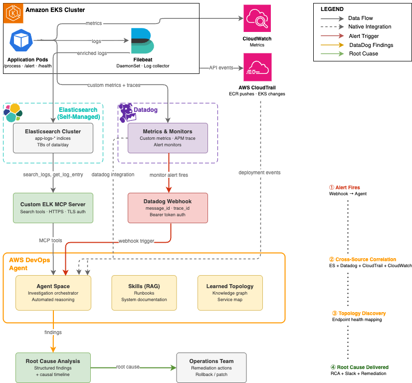
Figure 1: Automated root cause analysis pipeline — from Datadog alert to AWS DevOps Agent investigation across Elasticsearch, Datadog, and AWS CloudTrail
Implementation Walkthrough
The following walkthrough describes the end-to-end setup required to replicate the message ID traceability solution in your own environment.
Step 1: Configure EKS Cluster Access for AWS DevOps Agent
AWS DevOps Agent requires an access entry in each EKS cluster it will investigate. This enables the agent to describe Kubernetes objects, retrieve pod logs, and access cluster events.
- In the AWS DevOps Agent console, navigate to your Agent Space and select the Capabilities tab.
- Under the Cloud section, select the primary source and choose Edit. Note the Role Name shown in the Role Name field, this is the IAM role that requires EKS access.
- In the Amazon EKS console, select each cluster and open the Access tab.
- Under IAM Access Entries, choose Create to add a new access entry.
- Set the IAM Principal ARN to the Agent Space role noted in step 2.
- Under Access Policies, select
AmazonAIOpsAssistantPolicywith Cluster scope. Choose Add Policy, then Next. - Review and create the access entry.
At scale: For environments with 50+ clusters, use the AWS CLI, Terraform, or a GitOps pipeline to automate access entry creation across all clusters. The following CLI command creates an access entry for a single cluster:
aws eks create-access-entry --cluster-name <CLUSTER_NAME> --principal-arn <AGENTSPACE_ROLE_ARN> --region <REGION>aws eks associate-access-policy --cluster-name <CLUSTER_NAME> --principal-arn <AGENTSPACE_ROLE_ARN> --policy-arn arn:aws:eks::aws:cluster-access-policy/AmazonAIOpsAssistantPolicy --access-scope type=cluster --region <REGION>Step 2: Configure Datadog Integration in AWS DevOps Agent
AWS DevOps Agent includes native Datadog integration. Configuration requires your Datadog API credentials and designates the integration as a data source in the Agent Space. In the AWS DevOps Agent console, navigate to Integrations and choose Add Integration and follow the steps.
After configuration, AWS DevOps Agent can query Datadog metrics, monitors, and events during investigations. Custom application metrics (message throughput, error rates, processing status per message ID) are automatically accessible once the integration is active.
Step 3: Deploy and Configure the Custom ELK MCP Server
The Elasticsearch MCP server bridges AWS DevOps Agent to your self-managed Elasticsearch deployment. The MCP server is deployed as a publicly accessible endpoint with TLS authentication, enabling AWS DevOps Agent to call Elasticsearch APIs securely without requiring direct network access to the actual Elasticsearch/Kibana instances.
Note: For basic Elasticsearch integration, the official Elasticsearch MCP server provides a ready-to-use option. For this use case, we built a custom Python MCP server using FastMCP to expose investigation-specific tools — trace ID correlation, time-window log retrieval, and latency analysis — tailored to our message traceability workflow.
The custom server implementation provides the thirteen tools required for log search, index discovery, and aggregation.
| MCP Tool | Description |
|---|---|
search_logs |
Search by Lucene query string, time range, and log level |
get_error_summary |
Top recurring errors within a time window |
get_recent_logs |
Fetch most recent log entries from an index |
get_logs_by_service |
Filter logs by service or application name |
count_logs_by_level |
Breakdown of log counts by level (ERROR, WARN, INFO, DEBUG) |
get_slow_requests |
Find requests exceeding a latency threshold |
get_logs_around_time |
Fetch logs within ±N minutes of a specific timestamp |
search_by_trace_id |
Find all logs for a specific trace, request, or correlation ID |
get_unique_errors |
Get distinct error messages in a time window |
list_indices |
List all available Elasticsearch indices with doc counts and health |
get_index_stats |
Get size, document count, and health of a specific index |
get_logs_by_host |
Filter logs by the hostname that sent them via Filebeat |
get_logs_by_file |
Filter logs by the source log file path |
- Launch an Ubuntu instance (t4g.medium or larger) with a security group allowing inbound TCP 443 from AWS DevOps Agent service endpoints.Note: The single-instance deployment described here is intended for demonstration purposes and does not provide high availability. For production workloads requiring managed infrastructure, automatic scaling, and built-in resilience for your MCP servers, consider using Amazon Bedrock AgentCore Runtime.
- Install dependencies and obtain a TLS certificate:
sudo apt update &&sudo apt install -y python3 python3-venv certbot
python3 -m venv ~/elk-mcp-venv
source ~/elk-mcp-venv/bin/activate
pip install mcp elasticsearch uvicorn starlette
sudo certbot certonly --standalone -d elk-mcp.yourcompany.com - Create the MCP server. The key architectural decisions are: FastMCP for the Streamable HTTP transport, Starlette middleware for API key authentication, and environment variables for configuration:
import json, os from mcp.server.fastmcp import FastMCP from elasticsearch import Elasticsearch from starlette.middleware.base import BaseHTTPMiddleware from starlette.responses import JSONResponse ES_HOST = os.environ.get("ES_HOST", "http://localhost:9200") API_KEY = os.environ.get("MCP_API_KEY", "YOUR_API_KEY") es = Elasticsearch(hosts=[ES_HOST]) mcp = FastMCP("elk-logs", host="elk-mcp.yourcompany.com") # API key authentication middleware class APIKeyMiddleware(BaseHTTPMiddleware): async def dispatch(self, request, call_next): if request.headers.get("x-api-key") != API_KEY: return JSONResponse({"error": "Unauthorized"}, status_code=401) return await call_next(request) # Example: trace ID correlation tool @mcp.tool def search_by_trace_id(trace_id: str, index: str, size: int = 100) -> str: """Find all logs for a specific request or trace ID.""" result = es.search(index=index, body={ "query": {"multi_match": { "query": trace_id, "fields": ["trace_id", "request_id", "correlation_id", "traceId"] }}, "sort": [{"@timestamp": "asc"}], "size": size }) return json.dumps([h["_source"] for h in result["hits"]["hits"]], indent=2) # ... additional tools follow the same pattern app = mcp.streamable_http_app() app.add_middleware(APIKeyMiddleware) if __name__ == "__main__": import uvicorn uvicorn.run(app, host="0.0.0.0", port=443, ssl_keyfile="/etc/letsencrypt/live/elk-mcp.yourcompany.com/privkey.pem", ssl_certfile="/etc/letsencrypt/live/elk-mcp.yourcompany.com/fullchain.pem") - Start the server:
sudo -E ES_HOST=http://<ELASTICSEARCH_IP>:9200 MCP_API_KEY=<YOUR_API_KEY> nohup ~/elk-mcp-venv/bin/python ~/elk_mcp_server.py > ~/mcp.log 2>&1 & - Register in AWS DevOps Agent:
- In the AWS DevOps Agent console, navigate to Integrations -> Add MCP Integration.
- Enter the endpoint URL:
https://elk-mcp.yourcompany.com:443/mcp - Enter the API key for authentication.
- Verify the integration shows all available tools in the integration detail view.
- Add the MCP integration to your Agent Space under the Integrations tab.
Note: The MCP server must be publicly accessible over HTTPS. If your Elasticsearch cluster is in a private VPC, deploy the MCP server with network access to the cluster (e.g., in the same VPC or a peered VPC) while exposing only the MCP server endpoint publicly. Use security group rules to restrict access to AWS DevOps Agent’s known egress IP ranges where possible.
Step 4: Deploy the Application and Configure Filebeat on EKS
Filebeat runs as a Kubernetes DaemonSet on each EKS cluster, collecting pod logs and enriching them with Kubernetes metadata before forwarding to Elasticsearch. The following pipeline configuration ensures that message IDs and trace IDs are preserved as indexed fields, enabling efficient targeted queries during investigations.
- Clone the Repository and Build the Container Image:
# Clone the DevOps agent sample repository git clone https://github.com/aws-samples/Amazon-prometheus-bedrock-agent-example.git # Navigate to the smart demo directory cd devops-agent/smart-demo-main/ # Authenticate Docker to your ECR registry aws ecr get-login-password --region us-west-2 | docker login --username AWS --password-stdin <your-account-id>.dkr.ecr.us-west-2.amazonaws.com # Build the container image docker build -t sample-app . # Tag the image for ECR docker tag sample-app:latest <your-account-id>.dkr.ecr.us-west-2.amazonaws.com/smart-demp:latest # Push the image to ECR docker push <your-account-id>.dkr.ecr.us-west-2.amazonaws.com/smart-demp:latest - Deploy the Application to EKS:
# Deploy the sample application to EKS using Helm helm install sample-app ./helm --set image.repository=<your-account-id>.dkr.ecr.us-west-2.amazonaws.com/smart-demp --set image.tag=latest - Deploy Filebeat as DaemonSet:
# Navigate to the Filebeat directory
cd filebeat

# Apply the Filebeat ConfigMap (autodiscovery, JSON parsing, K8s metadata enrichment, Logstash output)
kubectl apply -f filebeat-configmap.yaml

# Deploy Filebeat as a DaemonSet on every node in the cluster
kubectl apply -f filebeat-ds.yaml
Step 5: Configure Datadog Webhook for Automatic Investigation Triggering
We will automatically trigger AWS DevOps Agent investigations when Datadog alerts fire. This eliminates the human latency between alert detection and investigation initiation.
Retrieve the AWS DevOps Agent webhook URL and secret:
- In the AWS DevOps Agent console, navigate to your Agent Space and open the Capabilities tab.
- Under the Webhook section, choose Configure, then Generate webhook.
- Save the webhook URL and HMAC secret. These credentials are used to authenticate webhook requests from Datadog.
In Datadog, configure a webhook integration:
- Navigate to Integrations -> Webhooks and create a new webhook.
- Set the URL to the AWS DevOps Agent webhook endpoint.
- Add the Authorization header with the bearer token from step 3.
- Configure the payload to include the message ID, trace ID, and alert context:
{ "title": "Message Processing Failure - $EVENT_TITLE", "description": "$EVENT_MSG", "alert_id": "$ALERT_ID", "alert_status": "$ALERT_STATUS", "timestamp": "$TIMESTAMP", "message_id": "$tags.message_id", "trace_id": "$tags.trace_id", "service": "$tags.service", "cluster": "$tags.cluster_name", "severity": "$ALERT_PRIORITY" } - Associate the webhook with the Datadog monitors that detect message processing failures by adding
@webhook-webhook-nameto the monitor notification message.
Step 6: Configure Agent Space Skills (Optional but Recommended)
AWS DevOps Agent Skills provide a Retrieval-Augmented Generation (RAG) knowledge base that gives the agent organization-specific context during investigations. Even a brief skills document (2-3 paragraphs) that identifies your application’s purpose, its key components, and its observability backends can reduce AWS DevOps Agent investigation time by helping the agent understand context before executing its first queries.
In our implementation, the skills document described the sample message-processing application, identified Elasticsearch as the logging backend, and identified Datadog as the metrics backend.
Real-World Investigation: Message Processing Failure Diagnosed in 6 Minutes
The following walkthrough and the scenario represent a common class of incident in distributed systems: a silent functional regression introduced through a new container image deployment that causes specific message types to fail processing without immediately obvious symptoms.
The Scenario
The production EKS cluster runs a message-processing application (sample-app) with four HTTP endpoints:
/health– Application health check/metrics– Prometheus metrics endpoint/process– Core message processing endpoint/alert– Alert notification endpoint (newly introduced in recent deployment)
A new container image was pushed to Amazon ECR with a new /alert endpoint. However, the endpoint implementation was incomplete when called; it returned an HTTP 404 response and silently dropped the associated message. The Filebeat DaemonSet collected pod logs and sent them into Elasticsearch. Datadog captured application metrics with message ID and trace ID labels. A Datadog monitor detected the elevated error rate and fired.
Phase 1: Alert Fires and Investigation Initiates (T+0:00)
At 14:52:57 UTC, a Datadog monitor detected an elevated rate of failed message processing requests on the /alert endpoint. The monitor fired a webhook to the AWS DevOps Agent endpoint with the alert payload context.
Within 10 seconds, the Agent read its investigation skills (sample-app-incident and triaging-3p-monitoring-alerts) and began planning the investigation approach.
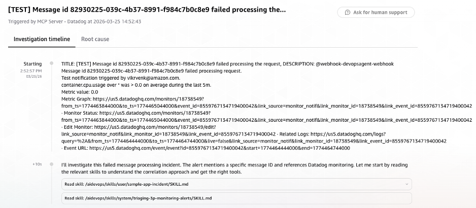
Figure 2: AWS DevOps Agent investigation initiated automatically via Datadog webhook, showing alert payload context and investigation skills loaded
Phase 2: Cross-Source Signal Correlation (T+0:10 – T+2:30)
AWS DevOps Agent began its investigation by using the message ID from the alert payload as its primary search key. It decided its investigation strategy: extract the trace_id from Elasticsearch using the message_id, get Datadog monitor details, and search for errors around the alert time.
Elasticsearch Log Search
The agent invoked the ELK MCP server to list available indices and identify the relevant log store for the message-processor application. It then executed a targeted search and identified the relevant Elasticsearch index (logs-2026.03.25):
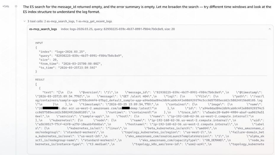
Figure 3: AWS DevOps Agent querying the ELK MCP Server to correlate message ID to trace ID across Elasticsearch indices
AWS DevOps Agent surfaced the Message ID to Trace ID correlation without any explicit cross-referencing instruction. It recognized the relationship from the log structure. At T+1:41, the DevOps Agent launched three parallel tasks simultaneously, rather than investigating sequentially.
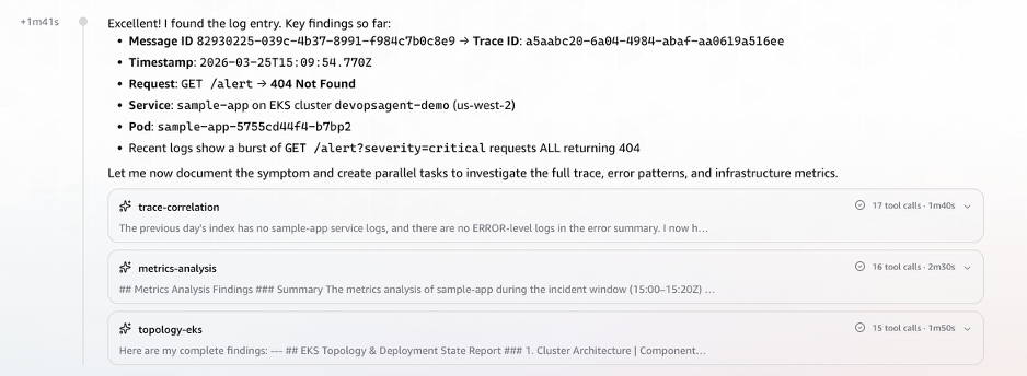 Figure 4: Trace ID successfully resolved from log structure, triggering three parallel investigation tasks
Datadog Metrics Correlation
Using the trace ID extracted from the Elasticsearch logs, the agent queried Datadog for correlated metrics. It retrieved CPU and memory utilization, pod count, restart metrics and enhanced metrics for request latency and errors.
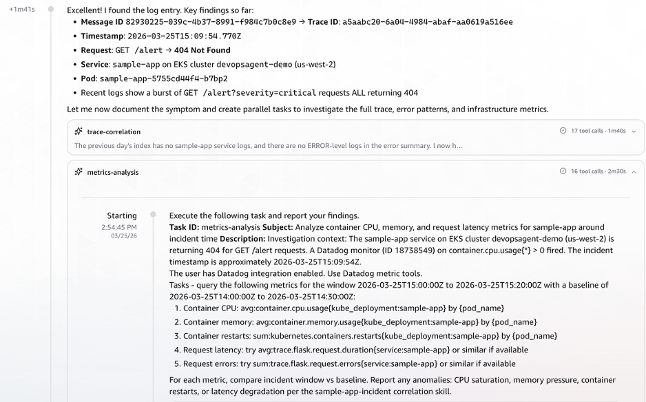
Figure 5: Datadog metrics correlation showing CPU, memory, pod restarts, and request latency retrieved using the extracted trace ID
AWS EKS Topology & CloudTrail Event Correlation
AWS DevOps Agent queried AWS CloudTrail for deployment and configuration change events in the time window preceding the alert.
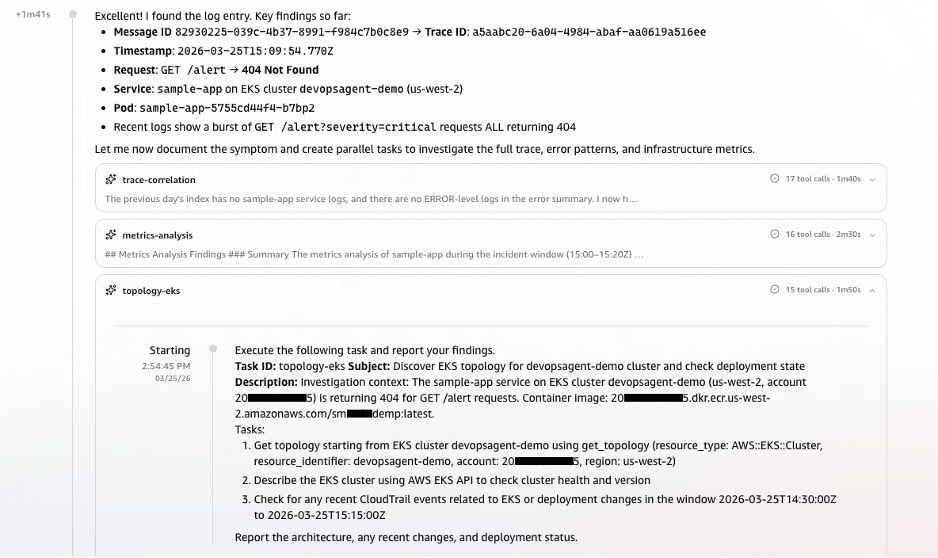
Figure 6: AWS CloudTrail event correlation identifying deployment and configuration changes in the alert time window
With the initial timeline established, AWS DevOps Agent examined all endpoints and their response patterns. This revealed that the application was fundamentally healthy, with three of four endpoints returned consistent 200 responses. However, it also revealed the anomaly was isolated to the /alert endpoint, which had never successfully served a request in its observable history.

Figure 7: AWS DevOps Agent endpoint analysis revealing isolated 404 failures on the /alert endpoint while other endpoints remain healthy
Phase 3: Observation Streaming from Parallel Tasks (T+2:30 – T+3:54)
As the three tasks ran simultaneously, observations streamed in chronologically:
T+2:58 – Observation: Anomalous CPU Behavior Signals Pod Disruption
The first sign of trouble came from pod tr8pl. Its CPU usage dropped sharply. Around the same time, two unfamiliar pods (85bx4, 7h4bd) briefly appeared with minimal CPU. Shortly after, three new pods (hclf9, b7bp2, g6gkc) spun up. This pattern of old pods dying, short-lived intermediaries, and fresh containers starting up pointed strongly toward a rolling deployment in progress.
T+3:04 – Observation: ECR Image Push Traced as the Trigger
With the deployment pattern established, the next question was: what initiated it? CloudTrail provided the answer. At 14:57:19 UTC, a user vik**** (via role nht-admin) pushed a new container image to ECR repository sm***demp:latest (ECR image tag). The timeline now made sense:
- ECR image push at 14:57:19 UTC
- Rolling deployment (pods replaced)
/alertendpoint 404 errors begin- Datadog alert fires
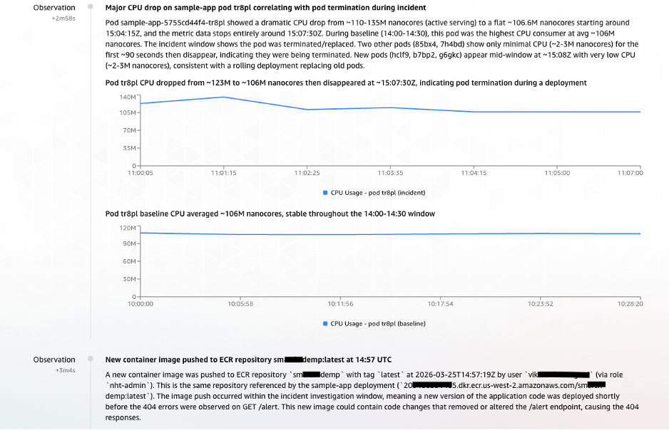
Figure 8: Parallel task observations streaming into AWS DevOps Agent – anomalous CPU behavior indicating pod disruption and CloudTrail evidence linking the ECR image push to the rolling deployment
Phase 4: Findings Documented – Causal Chain Established (T+3:55 – T+5:08)
At T+3:55, the Agent documented its first formal Finding (elevated from Observation):
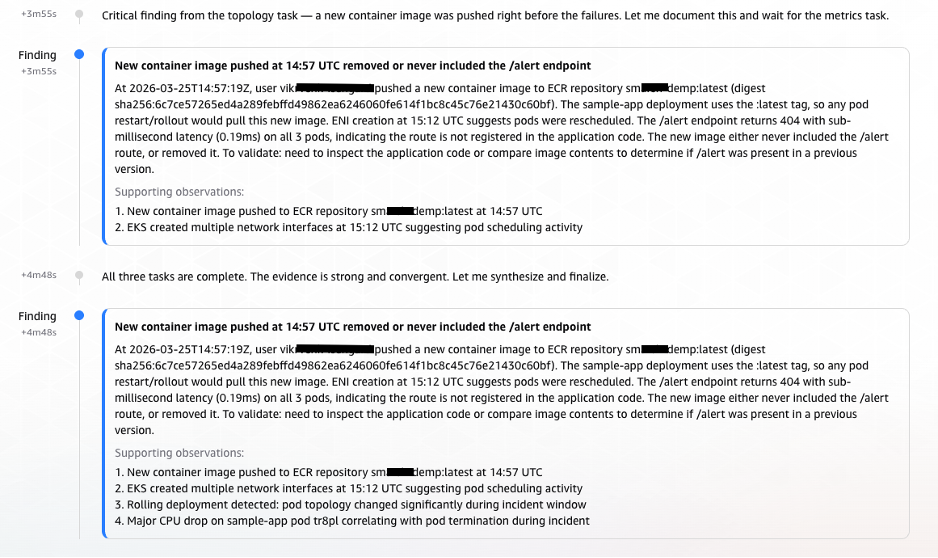
Figure 9: AWS DevOps Agent formal finding documenting the causal chain from ECR image push to alert endpoint failure
Phase 5: Root Cause Confirmation and Infrastructure Validation (T+5:10 – T+5:30)
AWS DevOps Agent validated infrastructure health. The complete absence of infrastructure issues, combined with the timeline evidence from CloudTrail and the historical 404 pattern on the /alert endpoint, allowed AWS DevOps Agent to deliver a high-confidence root cause identification.
At 14:58:12 UTC, exactly 5 minutes and 14 seconds (under 6 minutes) after the investigation began, AWS DevOps Agent delivered its root cause analysis:
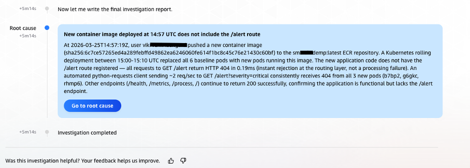
Figure 10: Final root cause analysis delivered by AWS DevOps Agent, identifying the incomplete alert endpoint in the newly deployed container image
Clean-up
Step 1: Delete the AWS DevOps Agent AgentSpace
- In the AWS DevOps Agent console, navigate to Agent Spaces.
- Select the Agent Space you created for this walkthrough.
- Remove all integrations (Datadog, ELK MCP Server) from the Agent Space by navigating to the Capabilities tab and choosing Remove for each.
- Choose Delete Agent Space from Actions dropdown and confirm the deletion.
Step 2: Terminate the Microservices and Delete the EKS Cluster
First, remove the application workloads and Filebeat DaemonSet deployed on the cluster:
# Uninstall the sample application Helm release
helm uninstall sample-app

# Delete the Filebeat DaemonSet and ConfigMap
kubectl delete -f filebeat/filebeat-ds.yaml
kubectl delete -f filebeat/filebeat-configmap.yaml
Once the workloads are removed, delete the EKS cluster.
Step 3: Terminate EC2 Instances
Terminate the EC2 instances hosting both the MCP server and the Elasticsearch cluster. You can do this from the AWS Management Console or the AWS CLI:
# Terminate the MCP server EC2 instance
aws ec2 terminate-instances --instance-ids <MCP_SERVER_INSTANCE_ID> --region <REGION>

# Terminate the Elasticsearch EC2 instances
aws ec2 terminate-instances --instance-ids <ELASTICSEARCH_INSTANCE_ID> --region <REGION>
Conclusion
Distributed systems have created a correlation problem that scales faster than the human capacity to solve it. As microservices architectures grow to span dozens of clusters, hundreds of services, and terabytes of daily telemetry, the manual investigation practices that worked at smaller scale become the primary obstacle in maintaining operational quality.
AWS DevOps Agent addresses this challenge at its root by automating the multi-source correlation that previously required experienced engineers working across multiple systems. The combination of native Datadog integration, custom ELK MCP server connectivity, and AWS CloudTrail access enables AWS DevOps Agent to build the complete picture of an incident: from the first metric anomaly, through the log evidence, to the deployment event that caused it. The scenario described in this post demonstrates that a message processing incident that previously consumed hours can be diagnosed to root cause in under six minutes automatically, without manual intervention, and with the full investigation documented for audit and learning purposes.
About the Authors

Bhuvan Jain
Bhuvan is a Senior Technical Account Manager at Amazon Web Services, supporting independent software vendor (ISV) customers. He is passionate about helping customers build Well-Architected solutions on AWS, with a focus on enterprise-scale networking. As a subject matter expert, Bhuvan offers guidance on designing network architectures that are highly available, resilient, and cost-effective. He holds a Master’s degree in Electrical and Computer Engineering from the University of Illinois at Chicago (UIC). In his free time, he enjoys playing basketball and volleyball, as well as watching movies and TV series.

Vikram Venkataraman
Vikram Venkataraman is a Principal Specialist Solutions Architect at Amazon Web Services. He helps customers modernize, scale, and adopt best practices for containerized workloads on Amazon EKS. With the emergence of AI-powered automation, Vikram has been actively working with customers to leverage AWS AI/ML services to solve complex operational challenges, streamline monitoring workflows, and enhance incident response through intelligent automation. He designed and built the POC architecture described in this post and is a co-author of the EKS knowledge graphs blog.


 Aswath Srinivasan is a Senior Search Engine Architect at Amazon Web Services currently based in Munich, Germany. With over 17 years of experience in various search technologies, Aswath currently focuses on OpenSearch. He is a search and open-source enthusiast and helps customers and the search community with their search problems.
 Jon Handler is a Senior Principal Solutions Architect at Amazon Web Services based in Palo Alto, CA. Jon works closely with OpenSearch and Amazon OpenSearch Service, providing help and guidance to a broad range of customers who have search and log analytics workloads that they want to move to the AWS Cloud. Prior to joining AWS, Jon’s career as a software developer included 4 years of coding a large-scale, ecommerce search engine. Jon holds a Bachelor of the Arts from the University of Pennsylvania, and a Master of Science and a PhD in Computer Science and Artificial Intelligence from Northwestern University.


 Viraj Phanse (