Next week, don’t miss AWS re:Invent, Dec. 1-5, 2025, for the latest AWS news, expert insights, and global cloud community connections! Our News Blog team is finalizing posts to introduce the most exciting launches from our service teams. If you’re joining us in person in Las Vegas, review the agenda, session catalog, and attendee guides before arriving. Can’t attend in person? Watch our Keynotes and Innovation Talks via livestream.
AWS CloudFormation StackSets offers deployment ordering for auto-deployment mode. You can define the sequence in which your stack instances automatically deploy across accounts and Regions.
AWS NAT Gateway supports Regional availability to create a single NAT Gateway that automatically expands and contracts across availability zones (AZs).
Deploying containerized applications to production requires navigating hundreds of configuration parameters across load balancers, auto scaling policies, networking, and security groups. This overhead delays time to market and diverts focus from core application development.
Today, I’m excited to announce Amazon ECS Express Mode, a new capability from Amazon Elastic Container Service (Amazon ECS) that helps you launch highly available, scalable containerized applications with a single command. ECS Express Mode automates infrastructure setup including domains, networking, load balancing, and auto scaling through simplified APIs. This means you can focus on building applications while deploying with confidence using Amazon Web Services (AWS) best practices. Furthermore, when your applications evolve and require advanced features, you can seamlessly configure and access the full capabilities of the resources, including Amazon ECS.
You can get started with Amazon ECS Express Mode by navigating to the Amazon ECS console.
Amazon ECS Express Mode provides a simplified interface to the Amazon ECS service resource with new integrations for creating commonly used resources across AWS. ECS Express Mode automatically provisions and configures ECS clusters, task definitions, Application Load Balancers, auto scaling policies, and Amazon Route 53 domains from a single entry point.
Getting started with ECS Express Mode Let me walk you through how to use Amazon ECS Express Mode. I’ll focus on the console experience, which provides the quickest way to deploy your containerized application.
For this example, I’m using a simple container image application running on Python with the Flask framework. Here’s the Dockerfile of my demo, which I have pushed to an Amazon Elastic Container Registry (Amazon ECR) repository:
On the Express Mode page, I choose Create. The interface is streamlined — I specify my container image URI from Amazon ECR, then select my task execution role and infrastructure role. If you don’t already have these roles, choose Create new role in the drop down to have one created for you from the AWS Identity and Access Management (IAM) managed policy.
If I want to customize the deployment, I can expand the Additional configurations section to define my cluster, container port, health check path, or environment variables.
In this section, I can also adjust CPU, memory, or scaling policies.
Setting up logs in Amazon CloudWatch Logs is something I always configure so I can troubleshoot my applications if needed. When I’m happy with the configurations, I choose Create.
After I choose Create, Express Mode automatically provisions a complete application stack, including an Amazon ECS service with AWS Fargate tasks, Application Load Balancer with health checks, auto scaling policies based on CPU utilization, security groups and networking configuration, and a custom domain with an AWS provided URL. I can also follow the progress in Timeline view on the Resources tab.
After it’s complete, I can see my application URL in the console and access my running application immediately.
After the application is created, I can see the details by visiting the specified cluster, or the default cluster if I didn’t specify one, in the ECS service to monitor performance, view logs, and manage the deployment.
When I need to update my application with a new container version, I can return to the console, select my Express service, and choose Update. I can use the interface to specify a new image URI or adjust resource allocations.
I find the entire experience reduces setup complexity while still giving me access to all the underlying resources when I need more advanced configurations.
Additional things to know Here are additional things about ECS Express Mode:
Availability – ECS Express Mode is available in all AWS Regions at launch.
Pricing – There is no additional charge to use Amazon ECS Express Mode. You pay for AWS resources created to launch and run your application.
Application Load Balancer sharing – The ALB created is automatically shared across up to 25 ECS services using host-header based listener rules. This helps distribute the cost of the ALB significantly.
Get started with Amazon ECS Express Mode through the Amazon ECS console. Learn more on the Amazon ECS documentation page.
You can use these open source solutions to develop applications faster, using up-to-date knowledge of Amazon Web Services (AWS) capabilities and configurations during the build and deployment process. Whether you’re writing code in your integrated development environment (IDE), or debugging production issues, these MCP servers support AI code assistants with deep understanding of Amazon ECS, Amazon EKS, and AWS Serverless capabilities, accelerating the journey from code to production. They work with popular AI-enabled IDEs, including Amazon Q Developer on the command line (CLI), to help you build and deploy applications using natural language commands.
The Amazon ECS MCP Server containerizes and deploys applications to Amazon ECS within minutes by configuring all relevant AWS resources, including load balancers, networking, auto-scaling, monitoring, Amazon ECS task definitions, and services. Using natural language instructions, you can manage cluster operations, implement auto-scaling strategies, and use real-time troubleshooting capabilities to identify and resolve deployment issues quickly.
For Kubernetes environments, the Amazon EKS MCP Server provides AI assistants with up-to-date, contextual information about your specific EKS environment. It offers access to the latest EKS features, knowledge base, and cluster state information. This gives AI code assistants more accurate, tailored guidance throughout the application lifecycle, from initial setup to production deployment.
The AWS Serverless MCP Server enhances the serverless development experience by providing AI coding assistants with comprehensive knowledge of serverless patterns, best practices, and AWS services. Using AWS Serverless Application Model Command Line Interface (AWS SAM CLI) integration, you can handle events and deploy infrastructure while implementing proven architectural patterns. This integration streamlines function lifecycles, service integrations, and operational requirements throughout your application development process. The server also provides contextual guidance for infrastructure as code decisions, AWS Lambda specific best practices, and event schemas for AWS Lambda event source mappings.
Let’s see it in action If this is your first time using AWS MCP servers, visit the Installation and Setup guide in the AWS Labs GitHub repository to installation instructions. Once installed, add the following MCP server configuration to your local setup:
Install Amazon Q for command line and add the configuration to ~/.aws/amazonq/mcp.json. If you’re already an Amazon Q CLI user, add only the configuration.
I want to create a backend application that automatically extracts metadata and understands the content of images and videos uploaded to an S3 bucket and stores that information in a database. I'd like to use a serverless system for processing. Could you generate everything I need, including the code and commands or steps to set up the necessary infrastructure, for it to work from start to finish? - Use 02_using_converse_api.ipynb as example code for the image and video understanding.
Amazon Q CLI identifies the necessary tools, including the MCP serverawslabs.aws-serverless-mcp-server. Through a single interaction, the AWS Serverless MCP server determines all requirements and best practices for building a robust architecture.
I ask to Amazon Q CLI that build and test the application, but encountered an error. Amazon Q CLI quickly resolved the issue using available tools. I verified success by checking the record created in the Amazon DynamoDB table and testing the application with the dog2.jpeg file.
To enhance video processing capabilities, I decided to migrate my media analysis application to a containerized architecture. I used this prompt:
I'd like you to create a simple application like the media analysis one, but instead of being serverless, it should be containerized. Please help me build it in a new CDK stack.
Amazon Q Developer begins building the application. I took advantage of this time to grab a coffee. When I returned to my desk, coffee in hand, I was pleasantly surprised to find the application ready. To ensure everything was up to current standards, I simply asked:
please review the code and all app using the awslabsecs_mcp_server tools
Amazon Q Developer CLI gives me a summary with all the improvements and a conclusion.
I ask it to make all the necessary changes, once ready I ask Amazon Q developer CLI to deploy it in my account, all using natural language.
After a few minutes, I review that I have a complete containerized application from the S3 bucket to all the necessary networking.
I ask Amazon Q developer CLI to test the app send it the-sea.mp4 video file and received a timed out error, so Amazon Q CLI decides to use the fetch_task_logs from awslabsecs_mcp_server tool to review the logs, identify the error and then fix it.
After a new deployment, I try it again, and the application successfully processed the video file
I can see the records in my Amazon DynamoDB table.
To test the Amazon EKS MCP server, I have code for a web app in the auction-website-main folder and I want to build a web robust app, for that I asked Amazon Q CLI to help me with this prompt:
Create a web application using the existing code in the auction-website-main folder. This application will grow, so I would like to create it in a new EKS cluster
Once the Docker file is created, Amazon Q CLI identifies generate_app_manifests from awslabseks_mcp_server as a reliable tool to create a Kubernetes manifests for the application.
Then create a new EKS cluster using the manage_eks_staks tool.
Once the app is ready, the Amazon Q CLI deploys it and gives me a summary of what it created.
I can see the cluster status in the console.
After a few minutes and resolving a couple of issues using the search_eks_troubleshoot_guide tool the application is ready to use.
Now I have a Kitties marketplace web app, deployed on Amazon EKS using only natural language commands through Amazon Q CLI.
Get started today Visit the AWS Labs GitHub repository to start using these AWS MCP servers and enhance your AI-powered developmen there. The repository includes implementation guides, example configurations, and additional specialized servers to run AWS Lambda function, which transforms your existing AWS Lambda functions into AI-accessible tools without code modifications, and Amazon Bedrock Knowledge Bases Retrieval MCP server, which provides seamless access to your Amazon Bedrock knowledge bases. Other AWS specialized servers in the repository include documentation, example configurations, and implementation guides to begin building applications with greater speed and reliability.
When running container workloads, you need to understand how software vulnerabilities create security risks for your resources. Until now, you could identify vulnerabilities in your Amazon Elastic Container Registry (Amazon ECR) images, but couldn’t determine if these images were active in containers or track their usage. With no visibility if these images were being used on running clusters, you had limited ability to prioritize fixes based on actual deployment and usage patterns.
Starting today, Amazon Inspector offers two new features that enhance vulnerability management, giving you a more comprehensive view of your container images. First, Amazon Inspector now maps Amazon ECR images to running containers, enabling security teams to prioritize vulnerabilities based on containers currently running in your environment. With these new capabilities, you can analyze vulnerabilities in your Amazon ECR images and prioritize findings based on whether they are currently running and when they last ran in your container environment. Additionally, you can see the cluster Amazon Resource Name (ARN), number EKS pods or ECS tasks where an image is deployed, helping you prioritize fixes based on usage and severity.
Second, we’re extending vulnerability scanning support to minimal base images including scratch, distroless, and Chainguard images, and extending support for additional ecosystems including Go toolchain, Oracle JDK & JRE, Amazon Corretto, Apache Tomcat, Apache httpd, WordPress (core, themes, plugins), and Puppeteer, helping teams maintain robust security even in highly optimized container environments.
Through continual monitoring and tracking of images running on containers, Amazon Inspector helps teams identify which container images are actively running in their environment and where they’re deployed, detecting Amazon ECR images running on containers in Amazon Elastic Container Service (Amazon ECS) and Amazon Elastic Kubernetes Service (Amazon EKS), and any associated vulnerabilities. This solution supports teams managing Amazon ECR images across single AWS accounts, cross-account scenarios, and AWS Organizations with delegated administrator capabilities, enabling centralized vulnerability management based on container images running patterns.
In the Amazon Inspector console, I navigate to General settings and select ECR scanning settings from the navigation panel. Here, I can configure the new Image re-scan mode settings by choosing between Last in-use date and Last pull date. I leave it as it is by default with Last in-usedate and set the Image last in use date to 14 days. These settings make it so that Inspector monitors my images based on when they were running in the last 14 days in my Amazon ECS or Amazon EKS environments. After applying these settings, Amazon Inspector starts tracking information about images running on containers and incorporating it into vulnerability findings, helping me focus on images actively running in containers in my environment.
After it’s configured, I can view information about images running on containers in the Details menu, where I can see last in-use and pull dates, along with EKS pods or ECS tasks count.
When selecting the number of Deployed ECS Tasks/EKS Pods, I can see the cluster ARN, last use dates, and Type for each image.
For cross-account visibility demonstration, I have a repository with EKS pods deployed in two accounts. In the Resources coverage menu, I navigate to Container repositories, select my repository name and choose the Image tag. As before, I can see the number of deployed EKS pods/ECS tasks.
When I select the number of deployed EKS pods/ECS tasks, I can see that it is running in a different account.
In the Findings menu, I can review any vulnerabilities, and by selecting one, I can find the Last in use date and Deployed ECS Tasks/EKS Pods involved in the vulnerability under Resource affected data, helping me prioritize remediation based on actual usage.
In the All Findings menu, you can now search for vulnerabilities within account management, using filters such as Account ID, Image in use count and Image last in use at.
Key features and considerations Monitoring based on container image lifecycle – Amazon Inspector now determines image activity based on: image push date ranging duration 14, 30, 60, 90, or 180 days or lifetime, image pull date from 14, 30, 60, 90, or 180 days, stopped duration from never to 14, 30, 60, 90, or 180 days and status of image running on the container. This flexibility lets organizations tailor their monitoring strategy based on actual container image usage rather than only repository events. For Amazon EKS and Amazon ECS workloads, last in use, push and pull duration are set to 14 days, which is now the default for new customers.
Image runtime-aware finding details – To help prioritize remediation efforts, each finding in Amazon Inspector now includes the lastInUseAt date and InUseCount, indicating when an image was last running on the containers and the number of deployed EKS pods/ ECS tasks currently using it. Amazon Inspector monitors both Amazon ECR last pull date data and images running on Amazon ECS tasks or Amazon EKS pods container data for all accounts, updating this information at least once daily. Amazon Inspector integrates these details into all findings reports and seamlessly works with Amazon EventBridge. You can filter findings based on the lastInUseAt field using rolling window or fixed range options, and you can filter images based on their last running date within the last 14, 30, 60, or 90 days.
Comprehensive security coverage – Amazon Inspector now provides unified vulnerability assessments for both traditional Linux distributions and minimal base images including scratch, distroless, and Chainguard images through a single service. This extended coverage eliminates the need for multiple scanning solutions while maintaining robust security practices across your entire container ecosystem, from traditional distributions to highly optimized container environments. The service streamlines security operations by providing comprehensive vulnerability management through a centralized platform, enabling efficient assessment of all container types.
Enhanced cross-account visibility – Security management across single accounts, cross-account setups, and AWS Organizations is now supported through delegated administrator capabilities. Amazon Inspector shares images running on container information within the same organization, which is particularly valuable for accounts maintaining golden image repositories. Amazon Inspector provides all ARNs for Amazon EKS and Amazon ECS clusters where images are running, if the resource belongs to the account with an API, providing comprehensive visibility across multiple AWS accounts. The system updates deployed EKS pods or ECS tasks information at least one time daily and automatically maintains accuracy as accounts join or leave the organization.
PS: Writing a blog post at AWS is always a team effort, even when you see only one name under the post title. In this case, I want to thank Nirali Desai, for her generous help with technical guidance, and expertise, which made this overview possible and comprehensive.
(This survey is hosted by an external company. AWS handles your information as described in the AWS Privacy Notice. AWS will own the data gathered via this survey and will not share the information collected with survey respondents.)
UNiDAYS is a fast, free digital platform that provides exclusive student offers and benefits to over 29 million verified members worldwide. With a rapidly growing user base and an increasing number of global partnerships, UNiDAYS recognized the need to enhance its platform’s performance to deliver a seamless consumer experience in geographic regions far from its original base of operations.
In this post, we share how UNiDAYS achieved AWS Region expansion in just 3 weeks using AWS services.
Business challenges
In response to growth opportunities, UNiDAYS faced a pressing business requirement: deliver low-latency responses and provide high availability for users across diverse geographic regions. At the same time, the platform needed to guarantee global data consistency while adhering to tight deadlines—all within just a few weeks. However, the existing monolithic application, although built on Amazon Web Services (AWS), wasn’t optimized for active-active multi-Region deployments.
The challenge was further complicated by the need to extend functionality from this legacy system, which used the AWS global network for improved user experience but fell short of meeting new business requirements. Re-architecting the entire platform to support multi-Region deployments within the given timeframe wasn’t feasible.
Solution overview
UNiDAYS opted to create complementary services tailored to these new requirements, using AWS services for a multi-Region, active-active architecture. The key services used included:
Amazon EventBridge – To enable asynchronous integration with existing systems through event-driven patterns
This approach allowed UNiDAYS to meet its latency, availability, and consistency goals while seamlessly integrating with existing infrastructure. The following diagram is the architecture for the solution.
Global delivery and resiliency
To provide the lowest latency and multi-Region resiliency, CloudFront was used with latency-based routing configured in Route 53. This routing directs requests to the Regional Application Load Balancers with the lowest latency, automatically providing resiliency in the event of Regional issues. Security was a key consideration. AWS WAF integration with CloudFront provided application-layer protection at the edge. Additional security measures included:
Custom HTTP headers on origin requests, enforced using Application Load Balancer listener rule conditions
Prefix lists to restrict access to Application Load Balancers, making sure that traffic originated from the intended CloudFront distributions
Rapid Regional deployment
The core infrastructure is deployed through Terraform, and applications are deployed using custom tooling that wraps AWS CloudFormation. This hybrid approach enabled rapid delivery by using existing patterns without disrupting established workflows. Resources were organized into tiers: platform, global, and Regional. Platform and global resources were deployed one time, and Regional resources were rolled out to each activated Region, streamlining expansion efforts.
One technical challenge involved CloudFormation exports, which are Regional by design. To address this, we implemented a custom CloudFormation macro to enable cross-Region access to exported values, providing consistency across deployments.
Amazon ECS enabled progressive application deployments within each Region, allowing teams to focus on scaling applications rather than managing infrastructure. For cost-efficiency, we used Spot Instances. During testing, container start-up latency was observed due to cross-Region image downloads from Amazon Elastic Container Registry (Amazon ECR). This issue was resolved by enabling private image replication in Amazon ECR so that container images were available locally in each Region. This solution significantly reduced start-up times, improving application responsiveness during deployments and scaling events.
Data consistency and performance
DynamoDB global tables were instrumental in providing eventual data consistency and Regional replication. With DynamoDB handling these aspects, we could focus on application logic.
The result was a substantial reduction in latency at key locations. For example, client-experienced latency in one Region dropped from approximately 200 milliseconds to 50 milliseconds upon deployment, as shown in the following screenshot.
Key technical hurdles
We addressed the following technical obstacles while developing the solution:
Cross-Region CloudFormation exports – CloudFormation exports are Regional by design. We addressed this by creating a custom CloudFormation macro to read exports across Regions.
Container start-up latency – Latency caused by cross-Region image downloads was mitigated by implementing Amazon ECR private image replication. This meant that container images were readily available in each Region, reducing deployment times and improving overall performance.
Security assurance – By using CloudFront, AWS WAF, and Application Load Balancer security features, we made sure that traffic and data remained secure.
Why AWS?
UNiDAYS chose AWS due to its comprehensive global infrastructure and robust service offerings, which allowed the platform to:
Seamlessly expand compute operations to Regions closer to its user base
Take advantage of a full stack of services for reliable, secure, and low-latency content delivery
Meet tight delivery deadlines without compromising on performance or security
Maintain flexibility where required, with the ability to use more managed services, which allowed a focus on our applications
Conclusion
By adopting a multi-Region, active-active architecture on AWS, UNiDAYS successfully met its business goals within only 3 weeks, rapidly expanding to new Regions while promoting platform resiliency. The solution improved latency by 75% in new Regions (from 200 milliseconds to 50 milliseconds), provided Regional data availability through DynamoDB global tables, and maintained 100% service uptime during resiliency tests, even in cases of Regional connectivity loss. Additionally, deployment velocity increased by over 40%, allowing faster feature releases and improved agility. This architecture not only provides a scalable and resilient platform for current operations but also establishes a strong foundation for future global expansion.
Learn more
Is your organization looking to expand into new Regions while maintaining performance and reliability?
Contact AWS experts to explore tailored solutions for your multi-Region strategy.
Agents for Amazon Bedrock now supports Provisioned Throughput pricing model – As agentic applications scale, they require higher input and output model throughput compared to on-demand limits. The Provisioned Throughput pricing model makes it possible to purchase model units for the specific base model.
Amazon EC2 Inf2 instances are now available in new regions – These instances are optimized for generative AI workloads and are generally available in the Asia Pacific (Sydney), Europe (London), Europe (Paris), Europe (Stockholm), and South America (Sao Paulo) Regions.
AWS Amplify Gen 2 is now generally available – AWS Amplify offers a code-first developer experience for building full-stack apps using TypeScript and enables developers to express app requirements like the data models, business logic, and authorization rules in TypeScript. AWS Amplify Gen 2 has added a number of features since the preview, including a new Amplify console with features such as custom domains, data management, and pull request (PR) previews.
Amazon Elastic Container Registry (ECR) adds pull through cache support for GitLab Container Registry – ECR customers can create a pull through cache rule that maps an upstream registry to a namespace in their private ECR registry. Once rule is configured, images can be pulled through ECR from GitLab Container Registry. ECR automatically creates new repositories for cached images and keeps them in-sync with the upstream registry.
Getting started with Amazon Q in VS Code – Check out this excellent step-by-step guide by Rohini Gaonkar that covers installing the extension for features like code completion chat, and productivity-boosting capabilities powered by generative AI.
AWS open source news and updates – My colleague Ricardo writes about open source projects, tools, and events from the AWS Community. Check out Ricardo’s page for the latest updates.
Upcoming AWS events Check your calendars and sign up for upcoming AWS events:
AWS Summits – Join free online and in-person events that bring the cloud computing community together to connect, collaborate, and learn about AWS. Register in your nearest city: Bengaluru (May 15–16), Seoul (May 16–17), Hong Kong (May 22), Milan (May 23), Stockholm (June 4), and Madrid (June 5).
AWS re:Inforce – Explore 2.5 days of immersive cloud security learning in the age of generative AI at AWS re:Inforce, June 10–12 in Pennsylvania.
AWS Community Days – Join community-led conferences that feature technical discussions, workshops, and hands-on labs led by expert AWS users and industry leaders from around the world: Turkey (May 18), Midwest | Columbus (June 13), Sri Lanka (June 27), Cameroon (July 13), Nigeria (August 24), and New York (August 28).
In this post, I’ll show how you can export software bills of materials (SBOMs) for your containers by using an AWS native service, Amazon Inspector, and visualize the SBOMs through Amazon QuickSight, providing a single-pane-of-glass view of your organization’s software supply chain.
The concept of a bill of materials (BOM) originated in the manufacturing industry in the early 1960s. It was used to keep track of the quantities of each material used to manufacture a completed product. If parts were found to be defective, engineers could then use the BOM to identify products that contained those parts. An SBOM extends this concept to software development, allowing engineers to keep track of vulnerable software packages and quickly remediate the vulnerabilities.
Today, most software includes open source components. A Synopsys study, Walking the Line: GitOps and Shift Left Security, shows that 8 in 10 organizations reported using open source software in their applications. Consider a scenario in which you specify an open source base image in your Dockerfile but don’t know what packages it contains. Although this practice can significantly improve developer productivity and efficiency, the decreased visibility makes it more difficult for your organization to manage risk effectively.
It’s important to track the software components and their versions that you use in your applications, because a single affected component used across multiple organizations could result in a major security impact. According to a Gartner report titled Gartner Report for SBOMs: Key Takeaways You Should know, by 2025, 60 percent of organizations building or procuring critical infrastructure software will mandate and standardize SBOMs in their software engineering practice, up from less than 20 percent in 2022. This will help provide much-needed visibility into software supply chain security.
Integrating SBOM workflows into the software development life cycle is just the first step—visualizing SBOMs and being able to search through them quickly is the next step. This post describes how to process the generated SBOMs and visualize them with Amazon QuickSight. AWS also recently added SBOM export capability in Amazon Inspector, which offers the ability to export SBOMs for Amazon Inspector monitored resources, including container images.
Why is vulnerability scanning not enough?
Scanning and monitoring vulnerable components that pose cybersecurity risks is known as vulnerability scanning, and is fundamental to organizations for ensuring a strong and solid security posture. Scanners usually rely on a database of known vulnerabilities, the most common being the Common Vulnerabilities and Exposures (CVE) database.
Identifying vulnerable components with a scanner can prevent an engineer from deploying affected applications into production. You can embed scanning into your continuous integration and continuous delivery (CI/CD) pipelines so that images with known vulnerabilities don’t get pushed into your image repository. However, what if a new vulnerability is discovered but has not been added to the CVE records yet? A good example of this is the Apache Log4j vulnerability, which was first disclosed on Nov 24, 2021 and only added as a CVE on Dec 1, 2021. This means that for 7 days, scanners that relied on the CVE system weren’t able to identify affected components within their organizations. This issue is known as a zero-day vulnerability. Being able to quickly identify vulnerable software components in your applications in such situations would allow you to assess the risk and come up with a mitigation plan without waiting for a vendor or supplier to provide a patch.
In addition, it’s also good hygiene for your organization to track usage of software packages, which provides visibility into your software supply chain. This can improve collaboration between developers, operations, and security teams, because they’ll have a common view of every software component and can collaborate effectively to address security threats.
In this post, I present a solution that uses the new Amazon Inspector feature to export SBOMs from container images, process them, and visualize the data in QuickSight. This gives you the ability to search through your software inventory on a dashboard and to use natural language queries through QuickSight Q, in order to look for vulnerabilities.
Solution overview
Figure 1 shows the architecture of the solution. It is fully serverless, meaning there is no underlying infrastructure you need to manage. This post uses a newly released feature within Amazon Inspector that provides the ability to export a consolidated SBOM for Amazon Inspector monitored resources across your organization in commonly used formats, including CycloneDx and SPDX.
Another Lambda function is invoked whenever a new JSON file is deposited. The function performs the data transformation steps and uploads the new file into a new S3 bucket.
Amazon Athena is then used to perform preliminary data exploration.
A dashboard on Amazon QuickSight displays SBOM data.
Implement the solution
This section describes how to deploy the solution architecture.
In this post, you’ll perform the following tasks:
Create S3 buckets and AWS KMS keys to store the SBOMs
Create QuickSight dashboards to identify libraries and packages
Use QuickSight Q to identify libraries and packages by using natural language queries
Deploy the CloudFormation stack
The AWS CloudFormation template we’ve provided provisions the S3 buckets that are required for the storage of raw SBOMs and transformed SBOMs, the Lambda functions necessary to initiate and process the SBOMs, and EventBridge rules to run the Lambda functions based on certain events. An empty repository is provisioned as part of the stack, but you can also use your own repository.
Browse to the CloudFormation service in your AWS account and choose Create Stack.
Upload the CloudFormation template you downloaded earlier.
For the next step, Specify stack details, enter a stack name.
You can keep the default value of sbom-inspector for EnvironmentName.
Specify the Amazon Resource Name (ARN) of the user or role to be the admin for the KMS key.
Deploy the stack.
Set up Amazon Inspector
If this is the first time you’re using Amazon Inspector, you need to activate the service. In the Getting started with Amazon Inspector topic in the Amazon Inspector User Guide, follow Step 1 to activate the service. This will take some time to complete.
Figure 2: Activate Amazon Inspector
SBOM invocation and processing Lambda functions
This solution uses two Lambda functions written in Python to perform the invocation task and the transformation task.
Invocation task — This function is run whenever a new image is pushed into Amazon ECR. It takes in the repository name and image tag variables and passes those into the create_sbom_export function in the SPDX format. This prevents duplicated SBOMs, which helps to keep the S3 data size small.
Transformation task — This function is run whenever a new file with the suffix .json is added to the raw S3 bucket. It creates two files, as follows:
It extracts information such as image ARN, account number, package, package version, operating system, and SHA from the SBOM and exports this data to the transformed S3 bucket under a folder named sbom/.
Because each package can have more than one CVE, this function also extracts the CVE from each package and stores it in the same bucket in a directory named cve/. Both files are exported in Apache Parquet so that the file is in a format that is optimized for queries by Amazon Athena.
Populate the AWS Glue Data Catalog
To populate the AWS Glue Data Catalog, you need to generate the SBOM files by using the Lambda functions that were created earlier.
To populate the AWS Glue Data Catalog
You can use an existing image, or you can continue on to create a sample image.
# Pull the nginx image from a public repo
docker pull public.ecr.aws/nginx/nginx:1.19.10-alpine-perl

docker tag public.ecr.aws/nginx/nginx:1.19.10-alpine-perl <ACCOUNT-ID>.dkr.ecr.us-east-1.amazonaws.com/sbom-inspector:nginxperl

# Authenticate to ECR, fill in your account id
aws ecr get-login-password --region us-east-1 | docker login --username AWS --password-stdin <ACCOUNT-ID>.dkr.ecr.us-east-1.amazonaws.com

# Push the image into ECR
docker push <ACCOUNT-ID>.dkr.ecr.us-east-1.amazonaws.com/sbom-inspector:nginxperl
An image is pushed into the Amazon ECR repository in your account. This invokes the Lambda functions that perform the SBOM export by using Amazon Inspector and converts the SBOM file to Parquet.
Verify that the Parquet files are in the transformed S3 bucket:
Browse to the S3 console and choose the bucket named sbom-inspector-<ACCOUNT-ID>-transformed. You can also track the invocation of each Lambda function in the Amazon CloudWatch log console.
After the transformation step is complete, you will see two folders (cve/ and sbom/)in the transformed S3 bucket. Choose the sbom folder. You will see the transformed Parquet file in it. If there are CVEs present, a similar file will appear in the cve folder.
The next step is to run an AWS Glue crawler to determine the format, schema, and associated properties of the raw data. You will need to crawl both folders in the transformed S3 bucket and store the schema in separate tables in the AWS Glue Data Catalog.
On the AWS Glue Service console, on the left navigation menu, choose Crawlers.
On the Crawlers page, choose Create crawler. This starts a series of pages that prompt you for the crawler details.
In the Crawler name field, enter sbom-crawler, and then choose Next.
Under Data sources, select Add a data source.
Now you need to point the crawler to your data. On the Add data source page, choose the Amazon S3 data store. This solution in this post doesn’t use a connection, so leave the Connection field blank if it’s visible.
For the option Location of S3 data, choose In this account. Then, for S3 path, enter the path where the crawler can find the sbom and cve data, which is s3://sbom-inspector-<ACCOUNT-ID>-transformed/sbom/ and s3://sbom-inspector-<ACCOUNT-ID>-transformed/cve/. Leave the rest as default and select Add an S3 data source.
Figure 3: Data source for AWS Glue crawler
The crawler needs permissions to access the data store and create objects in the Data Catalog. To configure these permissions, choose Create an IAM role. The AWS Identity and Access Management (IAM) role name starts with AWSGlueServiceRole-, and in the field, you enter the last part of the role name. Enter sbomcrawler, and then choose Next.
Crawlers create tables in your Data Catalog. Tables are contained in a database in the Data Catalog. To create a database, choose Add database. In the pop-up window, enter sbom-db for the database name, and then choose Create.
Verify the choices you made in the Add crawler wizard. If you see any mistakes, you can choose Back to return to previous pages and make changes. After you’ve reviewed the information, choose Finish to create the crawler.
Figure 4: Creation of the AWS Glue crawler
Select the newly created crawler and choose Run.
After the crawler runs successfully, verify that the table is created and the data schema is populated.
Figure 5: Table populated from the AWS Glue crawler
Set up Amazon Athena
Amazon Athena performs the initial data exploration and validation. Athena is a serverless interactive analytics service built on open source frameworks that supports open-table and file formats. Athena provides a simplified, flexible way to analyze data in sources like Amazon S3 by using standard SQL queries. If you are SQL proficient, you can query the data source directly; however, not everyone is familiar with SQL. In this section, you run a sample query and initialize the service so that it can used in QuickSight later on.
To start using Amazon Athena
In the AWS Management Console, navigate to the Athena console.
For Database, select sbom-db (or select the database you created earlier in the crawler).
Navigate to the Settings tab located at the top right corner of the console. For Query result location, select the Athena S3 bucket created from the CloudFormation template, sbom-inspector-<ACCOUNT-ID>-athena.
Keep the defaults for the rest of the settings. You can now return to the Query Editor and start writing and running your queries on the sbom-db database.
You can use the following sample query.
select package, packageversion, cve, sha, imagearn from sbom
left join cve
using (sha, package, packageversion)
where cve is not null;
Your Athena console should look similar to the screenshot in Figure 6.
Figure 6: Sample query with Amazon Athena
This query joins the two tables and selects only the packages with CVEs identified. Alternatively, you can choose to query for specific packages or identify the most common package used in your organization.
Amazon QuickSight is a serverless business intelligence service that is designed for the cloud. In this post, it serves as a dashboard that allows business users who are unfamiliar with SQL to identify zero-day vulnerabilities. This can also reduce the operational effort and time of having to look through several JSON documents to identify a single package across your image repositories. You can then share the dashboard across teams without having to share the underlying data.
QuickSight SPICE (Super-fast, Parallel, In-memory Calculation Engine) is an in-memory engine that QuickSight uses to perform advanced calculations. In a large organization where you could have millions of SBOM records stored in S3, importing your data into SPICE helps to reduce the time to process and serve the data. You can also use the feature to perform a scheduled refresh to obtain the latest data from S3.
QuickSight also has a feature called QuickSight Q. With QuickSightQ, you can use natural language to interact with your data. If this is the first time you are initializing QuickSight, subscribe to QuickSight and select Enterprise + Q. It will take roughly 20–30 minutes to initialize for the first time. Otherwise, if you are already using QuickSight, you will need to enable QuickSight Q by subscribing to it in the QuickSight console.
Finally, in QuickSight you can select different data sources, such as Amazon S3 and Athena, to create custom visualizations. In this post, we will use the two Athena tables as the data source to create a dashboard to keep track of the packages used in your organization and the resulting CVEs that come with them.
Prerequisites for setting up the QuickSight dashboard
This process will be used to create the QuickSight dashboard from a template already pre-provisioned through the command line interface (CLI). It also grants the necessary permissions for QuickSight to access the data source. You will need the following:
A QuickSight + Q subscription (only if you want to use the Q feature).
QuickSight permissions to Amazon S3 and Athena (enable these through the QuickSight security and permissions interface).
Set the default AWS Region where you want to deploy the QuickSight dashboard. This post assumes that you’re using the us-east-1 Region.
Create datasets
In QuickSight, create two datasets, one for the sbom table and another for the cve table.
In the QuickSight console, select the Dataset tab.
Choose Create dataset, and then select the Athena data source.
Name the data source sbom and choose Create data source.
Select the sbom table.
Choose Visualize to complete the dataset creation. (Delete the analyses automatically created for you because you will create your own analyses afterwards.)
Navigate back to the main QuickSight page and repeat steps 1–4 for the cve dataset.
Merge datasets
Next, merge the two datasets to create the combined dataset that you will use for the dashboard.
On the Datasets tab, edit the sbom dataset and add the cve dataset.
Set three join clauses, as follows:
Sha : Sha
Package : Package
Packageversion : Packageversion
Perform a left merge, which will append the cve ID to the package and package version in the sbom dataset.
Figure 7: Combining the sbom and cve datasets
Next, you will create a dashboard based on the combined sbom dataset.
Prepare configuration files
In your terminal, export the following variables. Substitute <QuickSight username> in the QS_USER_ARN variable with your own username, which can be found in the Amazon QuickSight console.
Validate that the variables are set properly. This is required for you to move on to the next step; otherwise you will run into errors.
echo ACCOUNT_ID is $ACCOUNT_ID || echo ACCOUNT_ID is not set
echo TEMPLATE_ID is $TEMPLATE_ID || echo TEMPLATE_ID is not set
echo QUICKSIGHT USER ARN is $QS_USER_ARN || echo QUICKSIGHT USER ARN is not set
echo QUICKSIGHT DATA ARN is $QS_DATA_ARN || echo QUICKSIGHT DATA ARN is not set
Next, use the following commands to create the dashboard from a predefined template and create the IAM permissions needed for the user to view the QuickSight dashboard.
Note: Run the following describe-dashboard command, and confirm that the response contains a status code of 200. The 200-status code means that the dashboard exists.
You should now be able to see the dashboard in your QuickSight console, similar to the one in Figure 8. It’s an interactive dashboard that shows you the number of vulnerable packages you have in your repositories and the specific CVEs that come with them. You can navigate to the specific image by selecting the CVE (middle right bar chart) or list images with a specific vulnerable package (bottom right bar chart).
Note: You won’t see the exact same graph as in Figure 8. It will change according to the image you pushed in.
Figure 8: QuickSight dashboard containing SBOM information
Alternatively, you can use QuickSight Q to extract the same information from your dataset through natural language. You will need to create a topic and add the dataset you added earlier. For detailed information on how to create a topic, see the Amazon QuickSight User Guide. After QuickSight Q has completed indexing the dataset, you can start to ask questions about your data.
Figure 9: Natural language query with QuickSight Q
Conclusion
This post discussed how you can use Amazon Inspector to export SBOMs to improve software supply chain transparency. Container SBOM export should be part of your supply chain mitigation strategy and monitored in an automated manner at scale.
Although it is a good practice to generate SBOMs, it would provide little value if there was no further analysis being done on them. This solution enables you to visualize your SBOM data through a dashboard and natural language, providing better visibility into your security posture. Additionally, this solution is also entirely serverless, meaning there are no agents or sidecars to set up.
Customers often ask for help with implementing Blue/Green deployments to Amazon Elastic Container Service (Amazon ECS) using AWS CodeDeploy. Their use cases usually involve cross-Region and cross-account deployment scenarios. These requirements are challenging enough on their own, but in addition to those, there are specific design decisions that need to be considered when using CodeDeploy. These include how to configure CodeDeploy, when and how to create CodeDeploy resources (such as Application and Deployment Group), and how to write code that can be used to deploy to any combination of account and Region.
Today, I will discuss those design decisions in detail and how to use CDK Pipelines to implement a self-mutating pipeline that deploys services to Amazon ECS in cross-account and cross-Region scenarios. At the end of this blog post, I also introduce a demo application, available in Java, that follows best practices for developing and deploying cloud infrastructure using AWS Cloud Development Kit (AWS CDK).
The Pipeline
CDK Pipelines is an opinionated construct library used for building pipelines with different deployment engines. It abstracts implementation details that developers or infrastructure engineers need to solve when implementing a cross-Region or cross-account pipeline. For example, in cross-Region scenarios, AWS CloudFormation needs artifacts to be replicated to the target Region. For that reason, AWS Key Management Service (AWS KMS) keys, an Amazon Simple Storage Service (Amazon S3) bucket, and policies need to be created for the secondary Region. This enables artifacts to be moved from one Region to another. In cross-account scenarios, CodeDeploy requires a cross-account role with access to the KMS key used to encrypt configuration files. This is the sort of detail that our customers want to avoid dealing with manually.
AWS CodeDeploy is a deployment service that automates application deployment across different scenarios. It deploys to Amazon EC2 instances, On-Premises instances, serverless Lambda functions, or Amazon ECS services. It integrates with AWS Identity and Access Management (AWS IAM), to implement access control to deploy or re-deploy old versions of an application. In the Blue/Green deployment type, it is possible to automate the rollback of a deployment using Amazon CloudWatch Alarms.
CDK Pipelines was designed to automate AWS CloudFormation deployments. Using AWS CDK, these CloudFormation deployments may include deploying application software to instances or containers. However, some customers prefer using CodeDeploy to deploy application software. In this blog post, CDK Pipelines will deploy using CodeDeploy instead of CloudFormation.
Design Considerations
In this post, I’m considering the use of CDK Pipelines to implement different use cases for deploying a service to any combination of accounts (single-account & cross-account) and regions (single-Region & cross-Region) using CodeDeploy. More specifically, there are four problems that need to be solved:
CodeDeploy Configuration
The most popular options for implementing a Blue/Green deployment type using CodeDeploy are using CloudFormation Hooks or using a CodeDeploy construct. I decided to operate CodeDeploy using its configuration files. This is a flexible design that doesn’t rely on using custom resources, which is another technique customers have used to solve this problem. On each run, a pipeline pushes a container to a repository on Amazon Elastic Container Registry (ECR) and creates a tag. CodeDeploy needs that information to deploy the container.
I recommend creating a pipeline action to scan the AWS CDK cloud assembly and retrieve the repository and tag information. The same action can create the CodeDeploy configuration files. Three configuration files are required to configure CodeDeploy: appspec.yaml, taskdef.json and imageDetail.json. This pipeline action should be executed before the CodeDeploy deployment action. I recommend creating template files for appspec.yaml and taskdef.json. The following script can be used to implement the pipeline action:
##
#!/bin/sh
#
# Action Configure AWS CodeDeploy
# It customizes the files template-appspec.yaml and template-taskdef.json to the environment
#
# Account = The target Account Id
# AppName = Name of the application
# StageName = Name of the stage
# Region = Name of the region (us-east-1, us-east-2)
# PipelineId = Id of the pipeline
# ServiceName = Name of the service. It will be used to define the role and the task definition name
#
# Primary output directory is codedeploy/. All the 3 files created (appspec.json, imageDetail.json and
# taskDef.json) will be located inside the codedeploy/ directory
#
##
Account=$1
Region=$2
AppName=$3
StageName=$4
PipelineId=$5
ServiceName=$6
repo_name=$(cat assembly*$PipelineId-$StageName/*.assets.json | jq -r '.dockerImages[] | .destinations[] | .repositoryName' | head -1)
tag_name=$(cat assembly*$PipelineId-$StageName/*.assets.json | jq -r '.dockerImages | to_entries[0].key')
echo ${repo_name}
echo ${tag_name}
printf '{"ImageURI":"%s"}' "$Account.dkr.ecr.$Region.amazonaws.com/${repo_name}:${tag_name}" > codedeploy/imageDetail.json
sed 's#APPLICATION#'$AppName'#g' codedeploy/template-appspec.yaml > codedeploy/appspec.yaml
sed 's#APPLICATION#'$AppName'#g' codedeploy/template-taskdef.json | sed 's#TASK_EXEC_ROLE#arn:aws:iam::'$Account':role/'$ServiceName'#g' | sed 's#fargate-task-definition#'$ServiceName'#g' > codedeploy/taskdef.json
cat codedeploy/appspec.yaml
cat codedeploy/taskdef.json
cat codedeploy/imageDetail.json
Using a Toolchain
A good strategy is to encapsulate the pipeline inside a Toolchain to abstract how to deploy to different accounts and regions. This helps decoupling clients from the details such as how the pipeline is created, how CodeDeploy is configured, and how cross-account and cross-Region deployments are implemented. To create the pipeline, deploy a Toolchain stack. Out-of-the-box, it allows different environments to be added as needed. Depending on the requirements, the pipeline may be customized to reflect the different stages or waves that different components might require. For more information, please refer to our best practices on how to automate safe, hands-off deployments and its reference implementation.
In detail, the Toolchain stack follows the builder pattern used throughout the CDK for Java. This is a convenience that allows complex objects to be created using a single statement:
In the statement above, the continuous deployment pipeline is created in the TOOLCHAIN_ACCOUNT and TOOLCHAIN_REGION. It implements a stage that builds the source code and creates the Java archive (JAR) using Apache Maven. The pipeline then creates a Docker image containing the JAR file.
The UAT stage will deploy the service to the SERVICE_ACCOUNT and SERVICE_REGION using the deployment configuration CANARY_10_PERCENT_5_MINUTES. This means 10 percent of the traffic is shifted in the first increment and the remaining 90 percent is deployed 5 minutes later.
To create additional deployment stages, you need a stage name, a CodeDeploy deployment configuration and an environment where it should deploy the service. As mentioned, the pipeline is, by default, a self-mutating pipeline. For example, to add a Prod stage, update the code that creates the Toolchain object and submit this change to the code repository. The pipeline will run and update itself adding a Prod stage after the UAT stage. Next, I show in detail the statement used to add a new Prod stage. The new stage deploys to the same account and Region as in the UAT environment:
In the statement above, the Prod stage will deploy new versions of the service using a CodeDeploy deployment configurationCANARY_10_PERCENT_5_MINUTES. It means that 10 percent of traffic is shifted in the first increment of 5 minutes. Then, it shifts the rest of the traffic to the new version of the application. Please refer to Organizing Your AWS Environment Using Multiple Accounts whitepaper for best-practices on how to isolate and manage your business applications.
Some customers might find this approach interesting and decide to provide this as an abstraction to their application development teams. In this case, I advise creating a construct that builds such a pipeline. Using a construct would allow for further customization. Examples are stages that promote quality assurance or deploy the service in a disaster recovery scenario.
The implementation creates a stack for the toolchain and another stack for each deployment stage. As an example, consider a toolchain created with a single deployment stage named UAT. After running successfully, the DemoToolchain and DemoService-UAT stacks should be created as in the next image:
CodeDeploy Application and Deployment Group
CodeDeploy configuration requires an application and a deployment group. Depending on the use case, you need to create these in the same or in a different account from the toolchain (pipeline). The pipeline includes the CodeDeploy deployment action that performs the blue/green deployment. My recommendation is to create the CodeDeploy application and deployment group as part of the Service stack. This approach allows to align the lifecycle of CodeDeploy application and deployment group with the related Service stack instance.
CodePipeline allows to create a CodeDeploy deployment action that references a non-existing CodeDeploy application and deployment group. This allows us to implement the following approach:
Toolchain stack deploys the pipeline with CodeDeploy deployment action referencing a non-existing CodeDeploy application and deployment group
When the pipeline executes, it first deploys the Service stack that creates the related CodeDeploy application and deployment group
The next pipeline action executes the CodeDeploy deployment action. When the pipeline executes the CodeDeploy deployment action, the related CodeDeploy application and deployment will already exist.
Below is the pipeline code that references the (initially non-existing) CodeDeploy application and deployment group.
To make this work, you should use the same application name and deployment group name values when creating the CodeDeploy deployment action in the pipeline and when creating the CodeDeploy application and deployment group in the Service stack (where the Amazon ECS infrastructure is deployed). This approach is necessary to avoid a circular dependency error when trying to create the CodeDeploy application and deployment group inside the Service stack and reference these objects to configure the CodeDeploy deployment action inside the pipeline. Below is the code that uses Service stack construct ID to name the CodeDeploy application and deployment group. I set the Service stack construct ID to the same name I used when creating the CodeDeploy deployment action in the pipeline.
CDK Pipelines creates roles and permissions the pipeline uses to execute deployments in different scenarios of regions and accounts. When using CodeDeploy in cross-account scenarios, CDK Pipelines deploys a cross-account support stack that creates a pipeline action role for the CodeDeploy action. This cross-account support stack is defined in a JSON file that needs to be published to the AWS CDK assets bucket in the target account. If the pipeline has the self-mutation feature on (default), the UpdatePipeline stage will do a cdk deploy to deploy changes to the pipeline. In cross-account scenarios, this deployment also involves deploying/updating the cross-account support stack. For this, the SelfMutate action in UpdatePipeline stage needs to assume CDK file-publishing and a deploy roles in the remote account.
The IAM role associated with the AWS CodeBuild project that runs the UpdatePipeline stage does not have these permissions by default. CDK Pipelines cannot grant these permissions automatically, because the information about the permissions that the cross-account stack needs is only available after the AWS CDK app finishes synthesizing. At that point, the permissions that the pipeline has are already locked-in. Hence, for cross-account scenarios, the toolchain should extend the permissions of the pipeline’s UpdatePipeline stage to include the file-publishing and deploy roles.
In cross-account environments it is possible to manually add these permissions to the UpdatePipeline stage. To accomplish that, the Toolchain stack may be used to hide this sort of implementation detail. In the end, a method like the one below can be used to add these missing permissions. For each different mapping of stage and environment in the pipeline it validates if the target account is different than the account where the pipeline is deployed. When the criteria is met, it should grant permission to the UpdatePipeline stage to assume CDK bootstrap roles (tagged using key aws-cdk:bootstrap-role) in the target account (with the tag value as file-publishing or deploy). The example below shows how to add permissions to the UpdatePipeline stage:
Let’s consider a pipeline that has a single deployment stage, UAT. The UAT stage deploys a DemoService. For that, it requires four actions: DemoService-UAT (Prepare and Deploy), ConfigureBlueGreenDeploy and Deploy.
The DemoService-UAT.Deploy action will create the ECS resources and the CodeDeploy application and deployment group. The ConfigureBlueGreenDeploy action will read the AWS CDK cloud assembly. It uses the configuration files to identify the Amazon Elastic Container Registry (Amazon ECR) repository and the container image tag pushed. The pipeline will send this information to the Deploy action. The Deploy action starts the deployment using CodeDeploy.
Solution Overview
As a convenience, I created an application, written in Java, that solves all these challenges and can be used as an example. The application deployment follows the same 5 steps for all deployment scenarios of account and Region, and this includes the scenarios represented in the following design:
Conclusion
In this post, I identified, explained and solved challenges associated with the creation of a pipeline that deploys a service to Amazon ECS using CodeDeploy in different combinations of accounts and regions. I also introduced a demo application that implements these recommendations. The sample code can be extended to implement more elaborate scenarios. These scenarios might include automated testing, automated deployment rollbacks, or disaster recovery. I wish you success in your transformative journey.
Amazon CodeCatalyst is an integrated service for software development teams adopting continuous integration and deployment (CI/CD) practices into their software development process. CodeCatalyst puts all of the tools that development teams need in one place, allowing for a unified experience for collaborating on, building, and releasing software. You can also integrate AWS resources with your projects by connecting your AWS accounts to your CodeCatalyst space. By managing all of the stages and aspects of your application lifecycle in one tool, you can deliver software quickly and confidently.
Introduction
Containerization has revolutionized the way we develop, deploy, and scale applications. With the rise of managed container services like Amazon Elastic Kubernetes Service (EKS), developers can leverage the power of Kubernetes without worrying about the underlying infrastructure. In this post, we will focus on how DevOps teams can use CodeCatalyst to build and deploy applications to EKS clusters.
CodeCatalyst offers a collection of pre-built actions that encapsulate common container-related tasks such as building and pushing a container image to an ECR and deploying a Kubernetes manifest. In this walkthrough, we will leverage two actions that can greatly simplify the container build and deployment process. We start by building a simple container image with the ‘Push to Amazon ECR’ action from CodeCatalyst labs. This action simplifies the process of building, tagging and pushing an image to an Amazon Elastic Container Registry (ECR). We will also utilize the ‘Deploy to Kubernetes cluster’ action from AWS for pushing our Kubernetes manifests with our updated image.
Figure 1: Architectural Diagram.
Prerequisites
To follow along with the post, you will need the following items:
The CodeCatalyst IAM role added to the aws-auth configMap for the EKS cluster
Walkthrough
In this walkthrough, we will build a simple Nginx based application and push this to an ECR, we will then build and deploy this image to an EKS cluster. The emphasis of this post, will be on how to translate a fairly common pattern with microservices applications to a CodeCatalyst workflow. At the end of the post, our workflow will look like so:
Figure 2: CodeCatalyst workflow.
Create the base workflow
To begin, we will create our workflow, in the CodeCatalyst project, Select CI/CD → Workflows → Create workflow:
Figure 3: Create workflow.
Leave the defaults for the Source Repository and Branch, select Create. We will have an empty workflow:
Figure 4: Empty workflow.
We can edit the workflow from within the CodeCatalyst console, or use a Dev Environment. We will create an initial commit of this workflow file, ignore any validation errors at this stage:
Figure 5: Creating Dev environment.
Connect to CodeCatalyst Dev Environment
For this post, we will use an AWS Cloud9 Dev Environment. Our first step is to connect to the Dev environment. Select Code → Dev Environments. If you do not already a Dev Instance, you can create an instance by selecting Create Dev Environment.
Figure 6: My Dev environment.
Create a CodeCatalyst secret
Prior to adding the code, we will add a CodeCatalyst secret that will be consumed by our workflow. Using CodeCatalyst secrets ensures that we do not store sensitive data in plaintext in our workflow file. To create the secrets in the CodeCatalyst console, browse to CICD -> Secrets. Select Create Secret with the following details:
Figure 7: Adding secrets.
Name: eks_cluster_name
Value: <Your EKS Cluster name>
Connect to the CodeCatalyst Dev Environment
We already have a Dev Environment so we will select Resume Instance. A new browser tab opens for the IDE and will be available in less than a minute. Once the IDE is ready, we can go ahead and start creating the Dockerfile and Kubernetes manifest that make up our application
mkdir WebApp
cat <<EOF > WebApp/Dockerfile
FROM nginx
RUN apt-get update && apt-get install -y curl
EOF
The previous command block creates our Dockerfile, which we will build in our CodeCatalyst workflow from an Nginx base image and installs cURL. Next, we will add our Kubernetes manifest file to create a Kubernetes deployment and service for our application:
Create a directory called Manifests and a file inside the directory called demo-app.yaml. Update the file with code for deployment and Kubernetes Service.
Figure 8: demo-app.yaml file.
The previous code block shows the Kubernetes manifest file for our deployment, along with a Kubernetes service. We modify the image value to include the URI for our ECR as this value is unique. Once we have created our Dockerfile and Kubernetes manifest, pull the latest changes to our repository, including our workflow file that we just created. In our environment, our repository is called eks-demo-app:
cd eks-demo-app && git pull
We can now edit this file in our IDE. In our example our workflow is Workflow_df84 , we will locate Workflow_df84.yaml in the .codecatalyst\workflows directory in our repository. From here we can double click on the file to launch in the IDE for editing:
Figure 9: workflow file in yaml format.
Add the build steps to workflow
We can assign our workflow a name and configure the action for our build phase. The code outlined in the following diagram is our CodeCatalyst workflow definition
Figure 10: Workflow updated with build phase.
Kustomize starts from here
Figure 11: Workflow updated with Kustomize.
Deployment starts from here
Figure 12: Workflow updated with Deployment phase.
The workflow will now contain two CodeCatalyst actions – PushtoAmazonECR which builds and pushes our container image to the ECR. We have also added a dependent stage DeploytoKubernetesCluster which deploys our Kubernetes manifest.
To save our changes we select File -> Save, we can then commit these to our git repository by typing the following at the terminal:
The previous command will commit and push our changes the CodeCatalyst source repository, as we have a branch trigger for main defined, this will trigger a run of the workflow. We can monitor the status of the workflow in the CodeCatalyst console by selecting CICD -> Workflows. Locate your workflow and click on Runs to view the status.
We will now have all two stages available, as depicted at the beginning of this walkthrough. We will now have a container image in our ECR along with the newly built image deployed to our EKS cluster.
Cleaning up
If you have been following along with this workflow, you should delete the resources that you have deployed to avoid further changes. First, delete the Amazon ECR repository and Amazon EKS cluster (along with associated IAM roles) using the AWS console. Second, delete the CodeCatalyst project by navigating to project settings and choosing to Delete Project.
Conclusion
In this post, we explained how teams can easily get started building, scanning, and deploying a microservice application to an EKS cluster using CodeCatalyst. We outlined the stages in our workflow that enabled us to achieve the end-to-end build and release cycle. We also demonstrated how to enhance the developer experience of integrating CodeCatalyst with our Cloud9 Dev Environment.
While developing with containers is becoming an increasingly popular way for deploying and scaling applications, there are still areas where improvements can be made. One of the main issues with scaling containerized applications is the long startup time, especially during scale up when newer instances need to be added. This issue can have a negative impact on the customer experience, for example when a website needs to scale out to serve additional traffic.
A research paper shows that container image downloads account for 76 percent of container startup time, but on average only 6.4 percent of the data is needed for the container to start doing useful work. Starting and scaling out containerized applications requires downloading container images from a remote container registry. This may introduce a non-trivial latency, as the entire image must be downloaded and unpacked before the applications can be started.
One solution to this problem is lazy loading (also known as asynchronous loading) container images. This approach downloads data from the container registry in parallel with the application startup, such as stargz-snapshotter, a project that aims to improve the overall container start time.
Last year, we introduced Seekable OCI (SOCI), a technology open sourced by Amazon Web Services (AWS) that enables container runtimes to implement lazy loading the container image to start applications faster without modifying the container images. As part of that effort, we open sourced SOCI Snapshotter, a snapshotter plugin that enables lazy loading with SOCI in containerd.
AWS Fargate Support for SOCI Today, I’m excited to share that AWS Fargate now supports Seekable OCI (SOCI), which helps applications deploy and scale out faster by enabling containers to start without waiting to download the entire container image. At launch, this new capability is available for Amazon Elastic Container Service (Amazon ECS) applications running on AWS Fargate.
Here’s a quick look to show how AWS Fargate support for SOCI works:
SOCI works by creating an index (SOCI index) of the files within an existing container image. This index is a key enabler to launching containers faster, providing the capability to extract an individual file from a container image without having to download the entire image. Your applications no longer need to wait to complete pulling and unpacking a container image before your applications start running. This allows you to deploy and scale out applications more quickly and reduce the rollout time for application updates.
A SOCI index is generated and stored separately from the container images. This means that your container images don’t need to be converted to use SOCI, therefore not breaking secure hash algorithm (SHA)-based security, such as container image signing. The index is then stored in the registry alongside the container image. At release, AWS Fargate support for SOCI works with Amazon Elastic Container Registry (Amazon ECR).
When you use Amazon ECS with AWS Fargate to run your SOCI-indexed containerized images, AWS Fargate automatically detects if a SOCI index for the image exists and starts the container without waiting for the entire image to be pulled. This also means that AWS Fargate will still continue to run container images that don’t have SOCI indexes.
Let’s Get Started There are two ways to create SOCI indexes for container images.
Use AWS SOCI Index Builder – AWS SOCI Index Builder is a serverless solution for indexing container images in the AWS Cloud. This AWS CloudFormation stack deploys an Amazon EventBridge rule to identify Amazon ECR action events and invoke an AWS Lambda function to match the defined filter. Then, another AWS Lambda function generates and pushes SOCI indexes to repositories in the Amazon ECR registry.
Create SOCI indexes manually – This approach provides more flexibility on in how the SOCI indexes are created, including for existing container images in Amazon ECR repositories. To create SOCI indexes, you can use the soci CLI provided by the soci-snapshotter project.
The AWS SOCI Index Builder provides you with an automated process to get started and build SOCI indexes for your container images. The sociCLI provides you with more flexibility around index generation and the ability to natively integrate index generation in your CI/CD pipelines.
In this article, I manually generate SOCI indexes using the soci CLI from the soci-snapshotter project.
Create a Repository and Push Container Images First, I create an Amazon ECR repository called pytorch-socifor my container image using AWS CLI.
For the sample application, I use a PyTorch training (CPU-based) container image from AWS Deep Learning Containers. I use the nerdctl CLI to pull the container image because, by default, the Docker Engine stores the container image in the Docker Engine image store, not the containerd image store.
Then, I tag the container image for the repository that I created in the previous step.
$ sudo nerdctl tag $SAMPLE_IMAGE $ECRSOCIURI
Next, I need to push the container image into the ECR repository.
$ sudo nerdctl push $ECRSOCIURI
At this point, my container image is already in my Amazon ECR repository.
Create SOCI Indexes Next, I need to create SOCI index.
A SOCI index is an artifact that enables lazy loading of container images. A SOCI index consists of 1) a SOCI index manifest and 2) a set of zTOCs. The following image illustrates the components in a SOCI index manifest, and how it refers to a container image manifest.
The SOCI index manifest contains the list of zTOCs and a reference to the image for which the manifest was generated. A zTOC, or table of contents for compressed data, consists of two parts:
TOC, a table of contents containing file metadata and the corresponding offset in the decompressed TAR archive.
zInfo, a collection of checkpoints representing the state of the compression engine at various points in the layer.
To learn more about the concept and term, please visit soci-snapshotterTerminology page.
Before I can create SOCI indexes, I need to install the sociCLI. To learn more about how to install the soci, visit Getting Started with soci-snapshotter.
To create SOCI indexes, I use the soci create command.
From the above output, I can see that sociCLI created zTOCs for four layers, which and this means only these four layers will be lazily pulled and the other container image layers will be downloaded in full before the container image starts. This is because there is less of a launch time impact in lazy loading very small container image layers. However, you can configure this behavior using the --min-layer-size flag when you run soci create.
Verify and Push SOCI Indexes The soci CLI also provides several commands that can help you to review the SOCI Indexes that have been generated.
To see a list of all index manifests, I can run the following command.
$ sudo soci index list

DIGEST                                                                     SIZE    IMAGE REF                                                                                   PLATFORM       MEDIA TYPE                                    CREATED
sha256:ea5c3489622d4e97d4ad5e300c8482c3d30b2be44a12c68779776014b15c5822    1931    xyz.dkr.ecr.us-east-1.amazonaws.com/pytorch-soci:latest                                     linux/amd64    application/vnd.oci.image.manifest.v1+json    10m4s ago
sha256:ea5c3489622d4e97d4ad5e300c8482c3d30b2be44a12c68779776014b15c5822    1931    763104351884.dkr.ecr.us-east-1.amazonaws.com/pytorch-training:1.5.1-cpu-py36-ubuntu16.04    linux/amd64    application/vnd.oci.image.manifest.v1+json    10m4s ago
While optional, if I need to see the list of zTOC, I can use the following command.
This series of zTOCs contains all of the information that SOCI needs to find a given file in a layer. To review the zTOC for each layer, I can use one of the digest sums from the preceding output and use the following command.
If I go to my Amazon ECR repository, I can verify the index is created. Here, I can see that two additional objects are listed alongside my container image: a SOCI Index and an Image index. The image index allows AWS Fargate to look up SOCI indexes associated with my container image.
Understanding SOCI Performance The main objective of SOCI is to minimize the required time to start containerized applications. To measure the performance of AWS Fargate lazy loading container images using SOCI, I need to understand how long it takes for my container images to start with SOCI and without SOCI.
To understand the duration needed for each container image to start, I can use metrics available from the DescribeTasks API on Amazon ECS. The first metric is createdAt, the timestamp for the time when the task was created and entered the PENDING state. The second metric is startedAt, the time when the task transitioned from the PENDING state to the RUNNING state.
For this, I have created another Amazon ECR repository using the same container image but without generating a SOCI index, called pytorch-without-soci. If I compare these container images, I have two additional objects in pytorch-soci(an image index and a SOCI index) that don’t exist in pytorch-without-soci.
Deploy and Run Applications To run the applications, I have created an Amazon ECS cluster called demo-pytorch-soci-cluster, a VPC and the required ECS task execution role. If you’re new to Amazon ECS, you can follow Getting started with Amazon ECS to be more familiar with how to deploy and run your containerized applications.
Now, let’s deploy and run both the container images with FARGATE as the launch type. I define five tasks for each pytorch-sociand pytorch-without-soci.
From the average aggregated delta time (between startedAt and createdAt) for each task, the pytorch-without-soci (without SOCI indexes) successfully ran after 129 seconds.
Next, I’m running same command but for pytorch-sociwhich comes with SOCI indexes.
Here, I see my container image with SOCI-enabled — pytorch-soci — was started 60 seconds after being created.
This means that running my sample application with SOCI indexes on AWS Fargate is approximately 50 percent faster compared to running without SOCI indexes.
It’s recommended to benchmark the startup and scaling-out time of your application with and without SOCI. This helps you to have a better understanding of how your application behaves and if your applications benefit from AWS Fargate support for SOCI.
Customer Voices During the private preview period, we heard lots of feedback from our customers about AWS Fargate support for SOCI. Here’s what our customers say:
Autodesk provides critical design, make, and operate software solutions across the architecture, engineering, construction, manufacturing, media, and entertainment industries. “SOCI has given us a 50% improvement in startup performance for our time-sensitive simulation workloads running on Amazon ECS with AWS Fargate. This allows our application to scale out faster, enabling us to quickly serve increased user demand and save on costs by reducing idle compute capacity. The AWS Partner Solution for creating the SOCI index is easy to configure and deploy.” – Boaz Brudner, Head of Innovyze SaaS Engineering, AI and Architecture, Autodesk.
Flywire is a global payments enablement and software company, on a mission to deliver the world’s most important and complex payments. “We run multi-step deployment pipelines on Amazon ECS with AWS Fargate which can take several minutes to complete. With SOCI, the total pipeline duration is reduced by over 50% without making any changes to our applications, or the deployment process. This allowed us to drastically reduce the rollout time for our application updates. For some of our larger images of over 750MB, SOCI improved the task startup time by more than 60%.”, Samuel Burgos, Sr. Cloud Security Engineer, Flywire.
Virtuoso is a leading software corporation that makes functional UI and end-to-end testing software. “SOCI has helped us reduce the lag between demand and availability of compute. We have very bursty workloads which our customers expect to start as fast as possible. SOCI helps our ECS tasks spin-up 40% faster, allowing us to quickly scale our application and reduce the pool of idle compute capacity, enabling us to deliver value more efficiently. Setting up SOCI was really easy. We opted to use the quick-start AWS Partner’s solution with which we could leave our build and deployment pipelines untouched.”, Mathew Hall, Head of Site Reliability Engineering, Virtuoso.
Things to Know Availability — AWS Fargate support for SOCI is available in all AWS Regions where Amazon ECS, AWS Fargate, and Amazon ECR are available.
Pricing — AWS Fargate support for SOCI is available at no additional cost and you will only be charged for storing the SOCI indexes in Amazon ECR.
Today I’m boarding a plane for Madrid. I will attend the AWS Summit Madrid this Thursday, and I will take Serverlesspresso with me. Serverlesspresso is a demo that we take to events, in where you can learn how to build event-driven architectures with serverless. If you are visiting an AWS Summit, most probably you will find one of our booths.
Last Week’s Launches Here are some launches that got my attention during the previous week.
AWS Glue – This week, AWS Glue made two important announcements. First, it announced the general availability of AWS Glue for Ray, a new data integration engine option for AWS Glue. Ray is a popular new open-source compute framework that helps developers to scale their Python workloads. In addition, AWS Glue announced AWS Glue Data Quality, a new capability that automatically measures and monitors data lake and data pipeline quality.
Other AWS News Some other updates and news that you may have missed:
Testing serverless applications – Testing serverless applications is one of those things that customers ask for guidance on from AWS. That is why we created a couple of new pages in Serverless Land to help you out. First, you can find the new guide on how to test serverless applications and then our new testing patterns collection, where you can find test integrations for you to use right away.
The Official AWS Podcast – Listen each week for updates on the latest AWS news and deep dives into exciting use cases. There are also official AWS podcasts in several languages. Check out the ones in French, German, Italian, and Spanish.
AWS Open-Source News and Updates – This is a newsletter curated by my colleague Ricardo to bring you the latest open-source projects, posts, events, and more.
Upcoming AWS Events Check your calendars and sign up for these AWS events:
AWS Silicon Innovation Day (June 21) – A one-day virtual event that focuses on AWS Silicon and how you can take advantage of AWS’s unique offerings. Learn more and register here.
AWS Global Summits – There are many summits going on right now around the world: Toronto (June 14), Madrid (June 15), and Milano (June 22).
AWS Community Day – Join a community-led conference run by AWS user group leaders in your region: Chicago (June 15), Manila (June 29–30), Chile (July 1), and Munich (September 14).
CDK Day – CDK Day is happening again this year on September 29. The call for papers for this event is open, and this year we are also accepting talks in Spanish. Submit your talk here.
That’s all for this week. Check back next Monday for another Week in Review!
AWS Graviton Processors are designed by AWS to deliver the best price performance for your cloud workloads running in Amazon Elastic Compute Cloud (Amazon EC2). Amazon CodeCatalyst recently added support to run workflow actions using on-demand or pre-provisioned compute powered by AWS Graviton processors. Customers can now access high performance AWS Graviton processors to build artifacts for Arm, or improve their price performance. In this post I will show you how to create a multi-architecture docker image using CodeCatalyst that can run on both amd64 and arm64 processors.
Background
Container images only run on a system with the same CPU architecture for which they were targeted. For example, an amd64 image runs on Intel and AMD processors, while an arm64 image runs on AWS Graviton. Note that amd64 and x86_64 are often used interchangeable, and I have chosen to use amd64 in this post. Rather than maintaining multiple repositories for each image type, you can combine variants for multiple architectures in the same repository. In addition, you can create a manifest describing which image to use for each architecture. This is known as multi-architecture, or multi-platform images.
Let us look at an example to further understand multi-arch images. In this screenshot from Amazon Elastic Container Registry (Amazon ECR), I have created two images for a simple hello-world application. One image is tagged latest-amd64 for AMD architectures and one tagged latest-arm64 for ARM architectures.
In addition, I have created an Image Index tagged latest. The image index is a map describing which image to use for each architecture. This allows my users to simply pull hello-world:latest and the index will identify the correct image based on the target platform. The image index contains the following manifest.
Now that I have explained what a multi-arch image is, I will explain how to create one in a CodeCatalyst workflow. A CodeCatalyst workflow is an automated procedure that describes how to build, test, and deploy your code as part of a continuous integration and continuous delivery (CI/CD) system. A workflow defines a series of steps, or actions, to take during a workflow run. Let’s get started.
Prerequisites
If you would like to follow along with this walkthrough, you will need:
In this walkthrough I will create a simple application using an Apache HTTP Server serving a static hello world page. The workload is inconsequential. I will focus on the process of building the container image using a CodeCatalyst workflow. The Workflow will build two container images, one for amd64 and one for arm64. The two build tasks will run in parallel on different compute architectures. When both builds are complete, the workflow will build the docker manifest. At the end of this post, my workflow will look like this.
Note that docker also offers a plugin called buildx that will allow you to build a multi-architecture image with a single command. In a real-world application, the workflow would also build the source code, run unit tests, etc. on each architecture. The sample application used in this post is so simple that there is no need to build and test the source code. Let’s examine the sample application now.
Sample Application
Initially the empty repository will only have a README.md file. By the end of this post, my repository will look like this.
I’ll begin by creating the file named index.html. I used the Create file button in CodeCatalyst console shown previously. My index.html file has the following content:
<html>
    <head>
        <title>Hello World!</title>
    </head>
    <body>
        <h1>Hello World!</h1>
        <p>Hello from a multi-architecture container created in CodeCatalyst.</p>
    </body>
</html>
I’ll also create a Dockerfile that contains two commands. The first command instructs Docker to build a new image from the Apache HTTP Server Project image called httpd. It is important to note that the httpd image already supports multiple architectures including amd64 and arm64. When creating a multi-architecture image, the base image must also support these architectures. The second command simply copies the index.html file above into the new image. My Dockerfile file has the following content.
FROM httpd
COPY ./index.html /usr/local/apache2/htdocs/
With the source code for my sample application complete, I can turn my attention to the workflow.
CI/CD Workflow
To create a new workflow, select CI/CD from navigation on the left and then select Workflows (1). Then, select Create workflow (2), leave the default options, and select Create (3).
If the workflow editor opens in YAML mode, select Visual to open the visual designer. Now, I can start adding actions to the workflow.
Build Action for the AMD64 Variant
I’ll begin by adding a build action for the amd64 container. Select “+ Actions” to open the actions list. Find the Build action and click “+” to add a new build action to the workflow.
On the Inputs tab, create three variable named AWS_DEFAULT_REGION,IMAGE_REPO_NAME, and IMAGE_TAG. Set the first two values equal to the region and **** name of your Amazon ECR repository**.** Set the third to latest-amd64. For example:
Now select the Configuration tab and rename the action docker_build_amd64. Select the Environment, AWS account connection, and Role for the associated AWS account where you created the Amazon ECR repository. For example:
Then, copy and paste the following code into the Shell commands. This code will build the image using the Dockerfile you created previously. Then, it logs into Amazon ECR, and finally, pushes the new image to ECR.
With the amd64 image complete, you can move on to the arm64 image.
Build Action for the ARM64 Variant
Add a second build action named docker_build_arm64 for the arm64 container. The configuration is nearly identical to the previous action with two minor changes. First, on the Inputs tab, I set the IMAGE_TAG to latest-arm64.
Second, on the Configuration tab, change the compute fleet to Linux.Arm64.Large. That is all you need to do to run your action on AWS Graviton. For example:
The Shell commands are identical to the arm64 build action. In addition, don’t forget to select the Environment, AWS account connection, and Role on the configuration tab. The complete configuration for the second action looks like this:
Now that you have a build action for the amd64 and arm64 images, you simply need to create a manifest file describing which image to use for each architecture.
Build Action for the Manifest
The final step in the workflow is to create the Docker manifest. Create a third build action named docker_manifest. You want this action to wait for the prior two actions to complete. Therefore, select the prior two actions from the Depends on drop down, like this:
Also configure four variables. AWS_DEFAULT_REGION and IMAGE_REPO_NAME are identical to the prior actions. In addition, IMAGE_TAG_AMD64 and IMAGE_TAG_ARM64 include the tags you created in the prior actions.
On the configuration tab, select the Environment, AWS account connection, and Role as you did in the prior actions. Then, copy and paste the following Shell commands.
I now have a complete CI/CD workflow that creates a container images for both amd64 and arm64. When I commit the changes, CodeCatalyst will execute my workflow, build the images, and push to ECR.
Cleanup
If you have been following along with this workflow, you should delete the resources you deployed so you do not continue to incur charges. First, delete the Amazon ECR repository using the AWS console. Second, delete the project from CodeCatalyst by navigating to Project settings and choosing Delete project.
Conclusion
AWS Graviton processors are custom-built by AWS to deliver the best price performance for cloud workloads. In this post I explained how to configure CodeCatalyst workflow actions to run on AWS Graviton. I used CodeCatalyst to create a workflow that builds a multi-architecture container image that can run on both amd64 and arm64 architectures. Get started building your multi-arch containers in Amazon CodeCatalyst today! You can read more about CodeCatalyst workflows in the documentation.
In the last post, OfferUp modernized its DevOps platform with Amazon EKS and Flagger to accelerate time to market, we talked about hypergrowth and the technical challenges encountered by OfferUp in its existing DevOps platform. As a reminder, we presented how OfferUp modernized its DevOps platform with Amazon Elastic Kubernetes Service (Amazon EKS) and Flagger to gain developer’s velocity, automate faster deployment, and achieve lower cost of ownership.
In this post, we discuss the technical steps to build a DevOps platform that enables the progressive deployment of microservices on Amazon Managed Amazon EKS. Progressive delivery exposes a new version of the software incrementally to ingress traffic and continuously measures the success rate of the metrics before allowing all of the new traffics to a newer version of the software. Flagger is the Graduate project of Cloud Native Computing Foundations (CNCF) that enables progressive canary delivery, along with bule/green and A/B Testing, while measuring metrics like HTTP/gRPC request success rate and latency. Flagger shifts and routes traffic between app versions using a service mesh or an Ingress controller
We leverage Gloo Ingress Controller for traffic routing, Prometheus, Datadog, and Amazon CloudWatch for application metrics analysis and Slack to send notification. Flagger will post messages to slack when a deployment has been initialized, when a new revision has been detected, and if the canary analysis failed or succeeded.
Prerequisite steps to build the modern DevOps platform
You need an AWS Account and AWS Identity and Access Management (IAM) user to build the DevOps platform. If you don’t have an AWS account with Administrator access, then create one now by clicking here. Create an IAM user and assign admin role. You can build this platform in any AWS region however, I will you us-west-1 region throughout this post. You can use a laptop (Mac or Windows) or an Amazon Elastic Compute Cloud (AmazonEC2) instance as a client machine to install all of the necessary software to build the GitOps platform. For this post, I launched an Amazon EC2 instance (with Amazon Linux2 AMI) as the client and install all of the prerequisite software. You need the awscli, git, eksctl, kubectl, and helm applications to build the GitOps platform. Here are the prerequisite steps,
Create a named profile(eks-devops) with the config and credentials file:
aws configure --profile eks-devops
AWS Access Key ID [None]: xxxxxxxxxxxxxxxxxxxxxx
AWS Secret Access Key [None]: xxxxxxxxxxxxxxxxxx
Default region name [None]: us-west-1
Default output format [None]:
View and verify your current IAM profile:
export AWS_PROFILE=eks-devops
aws sts get-caller-identity
If the Amazon EC2 instance doesn’t have git preinstalled, then install git in your Amazon EC2 instance:
sudo yum update -y
sudo yum install git -y
Check git version
git version
Git clone the repo and download all of the prerequisite software in the home directory.
Amazon ECR is a fully-managed container registry that makes it easy for developers to share and deploy container images and artifacts. ecr setup.sh script will create a new Amazon ECR repository and also push the podinfo images (6.0.0, 6.0.1, 6.0.2, 6.1.0, 6.1.5 and 6.1.6) to the Amazon ECR. Run ecr-setup.sh script with the parameter, “ECR repository name” (e.g. ps-flagger-repository) and region (e.g. us-west-1)
Technical steps to build the modern DevOps platform
This post shows you how to use the Gloo Edge ingress controller and Flagger to automate canary releases for progressive deployment on the Amazon EKS cluster. Flagger requires a Kubernetes cluster v1.16 or newer and Gloo Edge ingress 1.6.0 or newer. This post will provide a step-by-step approach to install the Amazon EKS cluster with managed node group, Gloo Edge ingress controller, and Flagger for Gloo in the Amazon EKS cluster. Now that the cluster, metrics infrastructure, and Flagger are installed, we can install the sample application itself. We’ll use the standard Podinfo application used in the Flagger project and the accompanying loadtester tool. The Flagger “podinfo” backend service will be called by Gloo’s “VirtualService”, which is the root routing object for the Gloo Gateway. A virtual service describes the set of routes to match for a set of domains. We’ll automate the canary promotion, with the new image of the “podinfo” service, from version 6.0.0 to version 6.0.1. We’ll also create a scenario by injecting an error for automated canary rollback while deploying version 6.0.2.
Use myeks-cluster.yaml to create your Amazon EKS cluster with managed nodegroup. myeks-cluster.yaml deployment file has “cluster name” value as ps-eks-66, region value as us-west-1, availabilityZones as [us-west-1a, us-west-1b], Kubernetes version as 1.24, and nodegroup Amazon EC2 instance type as m5.2xlarge. You can change this value if you want to build the cluster in a separate region or availability zone.
Create a namespace “gloo-system” and Install Gloo with Helm Chart. Gloo Edge is an Envoy-based Kubernetes-native ingress controller to facilitate and secure application traffic.
[Optional] If you’re using Datadog as a monitoring tool, then deploy Datadog agents as a DaemonSet using the Datadog Helm chart. Replace RELEASE_NAME and DATADOG_API_KEY accordingly. If you aren’t using Datadog, then skip this step. For this post, we leverage the Prometheus open-source monitoring tool.
Integrate Amazon EKS/ K8s Cluster with the Datadog Dashboard – go to the Datadog Console and add the Kubernetes integration.
[Optional] If you’re using Slack communication tool and have admin access, then Flagger can be configured to send alerts to the Slack chat platform by integrating the Slack alerting system with Flagger. If you don’t have admin access in Slack, then skip this step.
Create a namespace “apps”, and applications and load testing service will be deployed into this namespace.
kubectl create ns apps
Create a deployment and a horizontal pod autoscaler for your custom application or service for which canary deployment will be done.
kubectl -n apps apply -k app
kubectl get deployment -A
kubectl get hpa -n apps
Deploy the load testing service to generate traffic during the canary analysis.
kubectl -n apps apply -k tester
kubectl get deployment -A
kubectl get svc -n apps
Use apps-vs.yaml to create a Gloo virtual service definition that references a route table that will be generated by Flagger.
kubectl apply -f ./apps-vs.yaml
kubectl get vs -n apps
[Optional] If you have your own domain name, then open apps-vs.yaml in vi editor and replace podinfo.example.com with your own domain name to run the app in that domain.
Use canary.yaml to create a canary custom resource. Review the service, analysis, and metrics sections of the canary.yaml file.
kubectl apply -f ./canary.yaml
After a couple of seconds, Flagger will create the canary objects. When the bootstrap finishes, Flagger will set the canary status to “Initialized”.
kubectl -n apps get canary podinfo
NAME STATUS WEIGHT LASTTRANSITIONTIME
podinfo Initialized 0 2023-xx-xxTxx:xx:xxZ
Gloo automatically creates an ELB. Once the load balancer is provisioned and health checks pass, we can find the sample application at the load balancer’s public address. Note down the ELB’s Public address:
kubectl get svc -n gloo-system --field-selector 'metadata.name==gateway-proxy' -o=jsonpath='{.items[0].status.loadBalancer.ingress[0].hostname}{"\n"}'
Validate if your application is running, and you’ll see an output with version 6.0.0.
curl <load balancer’s public address> -H "Host:podinfo.example.com"
Trigger progressive deployments and monitor the status
You can Trigger a canary deployment by updating the application container image from 6.0.0 to 6.01.
kubectl -n apps set image deployment/podinfo podinfod=<ECR URI>:6.0.1
Flagger detects that the deployment revision changed and starts a new rollout.
kubectl -n apps describe canary/podinfo
Monitor all canaries, as the promoted status condition can have one of the following statuses: initialized, Waiting, Progressing, Promoting, Finalizing, Succeeded, and Failed.
watch kubectl get canaries --all-namespaces
curl < load balancer’s public address> -H "Host:podinfo.example.com"
Once canary is completed, validate your application. You can see that the version of the application is changed from 6.0.0 to 6.0.1.
[Optional] Open podinfo application from the laptop browser
Find out both of the IP addresses associated with load balancer.
dig < load balancer’s public address >
Open /etc/hosts file in the laptop and add both of the IPs of load balancer in the host file.
sudo vi /etc/hosts
<Public IP address of LB Target node> podinfo.example.com
e.g.
xx.xx.xxx.xxx podinfo.example.com
xx.xx.xxx.xxx podinfo.example.com
Type “podinfo.example.com” in your browser and you’ll find the application in form similar to this:
Figure 1: Greetings from podinfo v6.0.1
Automated rollback
While doing the canary analysis, you’ll generate HTTP 500 errors and high latency to check if Flagger pauses and rolls back the faulted version. Flagger performs automatic Rollback in the case of failure.
Introduce another canary deployment with podinfo image version 6.0.2 and monitor the status of the canary.
kubectl -n apps set image deployment/podinfo podinfod=<ECR URI>:6.0.2
Run HTTP 500 errors or a high-latency error from a separate terminal window.
Generate HTTP 500 errors:
watch curl -H 'Host:podinfo.example.com' <load balancer’s public address>/status/500
Generate high latency:
watch curl -H 'Host:podinfo.example.com' < load balancer’s public address >/delay/2
When the number of failed checks reaches the canary analysis threshold, the traffic is routed back to the primary, the canary is scaled to zero, and the rollout is marked as failed.
kubectl get canaries --all-namespaces
kubectl -n apps describe canary/podinfo
Cleanup
When you’re done experimenting, you can delete all of the resources created during this series to avoid any additional charges. Let’s walk through deleting all of the resources used.
Delete Amazon EKS Cluster After you’ve finished with the cluster and nodes that you created for this tutorial, you should clean up by deleting the cluster and nodes with the following command:
This post explained the process for setting up Amazon EKS cluster and how to leverage Flagger for progressive deployments along with Prometheus and Gloo Ingress Controller. You can enhance the deployments by integrating Flagger with Slack, Datadog, and webhook notifications for progressive deployments. Amazon EKS removes the undifferentiated heavy lifting of managing and updating the Kubernetes cluster. Managed node groups automate the provisioning and lifecycle management of worker nodes in an Amazon EKS cluster, which greatly simplifies operational activities such as new Kubernetes version deployments.
We encourage you to look into modernizing your DevOps platform from monolithic architecture to microservice-based architecture with Amazon EKS, and leverage Flagger with the right Ingress controller for secured and automated service releases.
Further Reading
Journey to adopt Cloud-Native DevOps platform Series #1: OfferUp modernized DevOps platform with Amazon EKS and Flagger to accelerate time to market
Genomics workflows are high-performance computing workloads. In Part 1 of this series, we demonstrated how life-science research teams can focus on scientific discovery without the associated heavy lifting. We used regenie for large genome-wide association studies. Our design pattern built on AWS Step Functions with AWS Batch and Amazon FSx for Lustre.
In Part 2, we explore genomics workloads with built-in workflow logic. Historically, running bioinformatics data pipelines was a manual and error-prone task. Over the last years, multiple workflow management systems have emerged. An example of these is the Snakemake workflow management system with Tibanna orchestration. We discuss the solution design and how you can fully automate the launch with Amazon Web Services (AWS).
Use case
We focus on the use case of Snakemake, an open-source utility for whole genome sequence mapping in directed acyclic graph (DAG) format. Snakemake uses Snakefiles to declare workflow steps and commands. A Snakefile extends Python syntax to declare workflow steps such as mapping data sets to DAG structure and identifying variants. Consult the Snakemake tutorial for further information on workflow rules.
Snakefiles provide an exception from the general design pattern and an alternative to granular modeling workflow logic in Amazon States Language. In our real-life use case, we used Tibanna to orchestrate Snakemake. Tibanna is an open-source, AWS-native software that runs bioinformatics data pipelines. It supports Snakefile syntax, plus other workflow languages, including Common Workflow Language and Workflow Description Language (WDL).
We recommend using Amazon Genomics CLI, if Tibanna is not needed for your use case, and Amazon Omics, if your workflow definitions are compliant with the supported WDL and Nextflow specifications.
The launched AWS Fargate task pulls the Snakefiles at launch time for each job and prepares the Snakemake initiation commands. Once the Snakefiles are downloaded on the Fargate task, the Snakemake head initiation command is invoked to begin launching jobs using Tibanna. Tibanna invokes a Step Functions state machine which orchestrates the launch of Snakemake on Amazon Elastic Compute Cloud (Amazon EC2).
Amazon CloudWatch provides a consolidated overview of performance metrics, including elapsed time, failed jobs, and error types. You can keep logs of your failed jobs in CloudWatch Logs (Figure 1). You can set up filters to match specific error types, plus create subscriptions to deliver a real-time stream of your log events to Amazon Kinesis or Lambda for further retry.
Figure 1. Solution architecture for Snakemake with Tibanna on AWS
Implementation considerations
Here, we describe some of the implementation considerations.
Creating Snakefiles
The launching point for the initiation depends on a Snakefile. Each Snakefile may contain one or more samples to be launched. The sheet resides in an S3 bucket. This adds flexibility and the ability to purge any sensitive or restrictive information after the job has been processed.
Invoking Tibanna
In order to launch Snakemake DAGs using Tibanna, we will need to set up a new Tibanna Unicorn. A Tibanna Unicorn is an Step Functions state machine and a corresponding Lambda function for provisioning EC2 instances.
The state machine runs the following sequence:
Create EC2 instance
Check EC2 status
Exit
After the Tibanna Unicorn has been created, we can start a Snakemake DAG using the following sample commands inside of the Fargate task.
The Snakemake command is used with the --tibanna flag to send launch requests to the Step Functions state machine in order to provision EC2 instances and run DAG tasks.
With this solution, each launch will automatically capture and retain start logs in a centralized location in Amazon CloudWatch Logs for tracing and auditing.
If there are issues during the launch of the Tibanna Step Function state machine, such as Amazon EC2 capacity limits, logs will be available in the S3 bucket that was specified during the Tibanna Unicorn creation process. There will be a file available in the format of <EXECUTION_ID>.log inside of the S3 bucket. This information is easily accessible via the command line interface. Use the following command to display specific log results or error messages.
tibanna log -j <EXECUTION_ID> -T
Retries and EC2 Spot Instances
We advise to use Amazon EC2 Spot Instances, if possible, for additional cost savings. This option is available in the --tibanna-config arguments with the setting spot_instance=true.
This is optional, and you need to create retry logic in the event a Spot Instance gets reclaimed. You can include --retries=3 in your Tibanna launch command. This would ensure all rules are retried three times. You can also specify the number of retries for individual rules when defining the Snakemake DAG definition; for example:
If EC2 Spot Instance capacity is hit, you can automatically switch to using EC2 On-Demand Instances instead. Add the behavior_on_capacity_limit argument and set retry_without_spot=true.
To initiate jobs on ParallelCluster, install the AWS Systems Manager agent on the head node. This is the launching point into the cluster and used for submitting jobs to the initiation queue. Systems Manager is a secure way to remotely invoke commands on an EC2 instance without the need for SSH access. You can restrict access to your EC2 instance through IAM policies.
Conclusion
In this blog post, we demonstrated how life-science research teams can simplify the launch of Snakemake using AWS. We used Snakefiles and Tibanna to orchestrate workflow steps. Snakefiles provide an exception from the general design pattern and an alternative to Amazon States Language. File uploads to Amazon S3 served as our launching point for workflow initiations.
Stay tuned for Part 3 of this series, in which we create a job manager that administrates multiple workflows.
Genomics workflows are high-performance computing workloads. Traditionally, they run on-premises with a collection of scripts. Scientists run and manage these workflows manually, which slows down the product development lifecycle. Scientists spend time to administer workflows and handle errors on a day-to-day basis. They also lack sufficient compute capacity on-premises.
In this blog post, we demonstrate how life sciences companies can use Amazon Web Services (AWS) to remove the traditional heavy lifting associated with genomic studies. We use AWS Step Functions to orchestrate workflow steps, including error handling. With AWS Batch, we horizontally scale-out the analytic tasks for optimal performance. This allows genome scientists to focus on scientific discovery while AWS runs their workflows.
Use case
Workflow systems used for genomic analysis include Cromwell, Nextflow, and regenie. These high-performance computing systems share the following requirements:
Fast access to datasets at petabyte scale
Parallel task distribution, with horizontal compute scale-out
Data processing in batches following a specific sequence of data analysis steps, which vary by use case
We explore the use case of regenie. regenie is a common, open-source utility for whole-genome regression modelling of large genome-wide association studies (GWAS). GWAS compare DNA datasets of individuals with a specific trait or disease. The intent is to associate the identified trait/disease with DNA variants. Among other positive results, this helps identify at-risk patients, plus testing and prevention opportunities.
The first step searches for variants associated with a specific trait in a dataset of individuals with the trait, in order to create a whole-genome regression model that captures the variance.
The second step validates for association with the identified variants against a larger dataset, typically in the scale of petabytes, and launches a sequence of tasks run on data batches.
Solution overview
The entire regenie workflow and associated tasks of attaching and deleting file-share access to sample data, as well as spinning up compute instances for parallel computing, can be orchestrated with Step Functions. We use Amazon FSx for Lustre as a high-performance, transient file system providing file access to the datasets stored in an Amazon Simple Storage Service (Amazon S3) bucket. AWS Batch allows us to programmatically spin up multiple Amazon Elastic Compute Cloud (Amazon EC2) instances on which regenie can distribute parallel computing tasks. We do this with an AWS Lambda function that calculates the number of required batch jobs based on the requested size of samples per batch.
regenie is available as Docker image on GitHub. We push the image to Amazon Elastic Container Registry from which AWS Batch can pull it with the creation of new jobs at launch time. The Step Functions state machine is initiated by a Lambda function, with interactive user input. In the past, scientists have also directly interacted with the Step Functions API via the AWS Management Console or by running start-execution in the AWS Command Line Interface and passing a JSON file with the input parameters.
Amazon CloudWatch provides a consolidated overview of performance metrics, including elapsed time, failed jobs, and error types. You can keep logs of your failed jobs in Amazon CloudWatch Logs (Figure 1). You can set up filters to match specific error types, plus create subscriptions to deliver a real-time stream of your log events to Amazon Kinesis or AWS Lambda for further retry.
Figure 1. Solution overview for automating regenie workflows on AWS
Alternatively, the Step Functions workflow triggers another Lambda function, which puts failed job logs to Amazon DynamoDB. In the past, we have used this to ease data access and manipulation via the AWS management console. Scientists updated table items and DynamoDB Streams initiated the retry.
Workflow automation
With each invocation, Step Functions initiates a new instance of the state machine. AWS documentation provides an overview of the API quotas. Step Functions allows the modeling of the entire workflow, including custom application error handling. Map state improves performance by parallelizing workflow branches.
The state machine initiates the build of the file system and, once it’s ready, creates a data repository association with the sample data stored on Amazon S3. It waits until the data repository association is complete and proceeds with the calculation of batch jobs, based on a user-defined number of samples to be processed per batch job (Figure 2). This is essential to determine the amount of compute instances required for data processing.
Next, the state machine builds the commands to launch the regenie steps, as requested by the user, and submit the jobs for AWS Batch (Figure 3). The workflow checks if a specific version of regenie was requested by the user, otherwise, it defaults to the version of regenie on the container.
Then, we build the commands to initiate the two regenie steps. Step 2 may need to run in multiple iterations on different datasets (more often than Step 1). This is also determined with user input at initiation of the workflow. With Step Functions, we create runner logic to build the set of commands dynamically. This pattern is applicable to other scientific workloads, as well.
Figure 3. AWS Step Functions workflow for regenie: prepare and submit jobs
Once jobs are submitted, the workflow proceeds (by default) with the initiation of Step 1 of regenie; if requested by the user, the workflow will proceed directly to step 2 (Figure 4).
Any errors during batch launch leading to the failure of a job are passed, in this case, to a Lambda function. We configure the Lambda function to write the failed job logs to Amazon DynamoDB or as S3 objects.
Figure 4. AWS Step Functions workflow for regenie: launch jobs
Finally, the Step Functions workflow checks for pending errors and confirms that all jobs have finished their initiation. Then, it deletes the file system and data repository association and ends the workflow instance (Figure 5).
Figure 5. AWS Step Functions workflow for regenie: complete error handling and delete file system
As demonstrated, we can automate the entire process, from data access to verifying job completion and cleaning-up transient resources. This removes manual error handling and retry, plus reduces the overall cost of running regenie workflows. We also showed in Figure 3 that you can build commands dynamically for different scientific workloads.
Conclusion
In this blog post, we addressed a common pain point in the daily work of life sciences research teams. Traditionally, they had to run genomics workflows manually on limited compute capacity. Moving those workflows to AWS eliminates the heavy lifting of running scripts manually and expedites computational cycles. This allows research teams to stay focused on scientific discovery.
We recommend a thorough performance testing when setting up your genomics workflows. This includes determining the most suitable EC2 instance size. Some workflows, such as regenie, are single-threaded and benefit from horizontal scale-out of the number of instances but not from vertical scale-out of instance sizes.
AWS Glue is a fully managed serverless service that allows you to process data coming through different data sources at scale. You can use AWS Glue jobs for various use cases such as data ingestion, preprocessing, enrichment, and data integration from different data sources. AWS Glue version 3.0, the latest version of AWS Glue Spark jobs, provides a performance-optimized Apache Spark 3.1 runtime experience for batch and stream processing.
You can author AWS Glue jobs in different ways. If you prefer coding, AWS Glue allows you to write Python/Scala source code with the AWS Glue ETL library. If you prefer interactive scripting, AWS Glue interactive sessions and AWS Glue Studio notebooks helps you to write scripts in notebooks by inspecting and visualizing the data. If you prefer a graphical interface rather than coding, AWS Glue Studio helps you author data integration jobs visually without writing code.
For a production-ready data platform, a development process and CI/CD pipeline for AWS Glue jobs is key. We understand the huge demand for developing and testing AWS Glue jobs where you prefer to have flexibility, a local laptop, a Docker container on Amazon Elastic Compute Cloud (Amazon EC2), and so on. You can achieve that by using AWS Glue Docker images hosted on Docker Hub or the Amazon Elastic Container Registry (Amazon ECR) Public Gallery. The Docker images help you set up your development environment with additional utilities. You can use your preferred IDE, notebook, or REPL using the AWS Glue ETL library.
This post is a continuation of blog post “Developing AWS Glue ETL jobs locally using a container“. While the earlier post introduced the pattern of development for AWS Glue ETL Jobs on a Docker container using a Docker image, this post focuses on how to develop and test AWS Glue version 3.0 jobs using the same approach.
AWS Glue version 3.0 – public.ecr.aws/glue/aws-glue-libs:glue_libs_3.0.0_image_01
AWS Glue version 2.0 – public.ecr.aws/glue/aws-glue-libs:glue_libs_2.0.0_image_01
Note: AWS Glue Docker images are x86_64 compatible and arm64 hosts are currently not supported.
In this post, we use amazon/aws-glue-libs:glue_libs_3.0.0_image_01 and run the container on a local machine (Mac, Windows, or Linux). This container image has been tested for AWS Glue version 3.0 Spark jobs. The image contains the following:
Other library dependencies (the same as the ones of the AWS Glue job system)
To set up your container, you pull the image from Docker Hub and then run the container. We demonstrate how to run your container with the following methods, depending on your requirements:
spark-submit
REPL shell (pyspark)
pytest
JupyterLab
Visual Studio Code
Prerequisites
Before you start, make sure that Docker is installed and the Docker daemon is running. For installation instructions, see the Docker documentation for Mac, Windows, or Linux. Also make sure that you have at least 7 GB of disk space for the image on the host running Docker.
These variables are used in the docker run command below. The sample code (sample.py) used in the spark-submit command below is included in the appendix at the end of this post.
Run the following command to run the spark-submit command on the container to submit a new Spark application:
You can run a REPL (read-eval-print loop) shell for interactive development. Run the following command to run the pyspark command on the container to start the REPL shell:
$ docker run -it -v ~/.aws:/home/glue_user/.aws -e AWS_PROFILE=$PROFILE_NAME -e DISABLE_SSL=true --rm -p 4040:4040 -p 18080:18080 --name glue_pyspark amazon/aws-glue-libs:glue_libs_3.0.0_image_01 pyspark
...
 ____ __
 / __/__ ___ _____/ /__
 _\ \/ _ \/ _ `/ __/ '_/
 /__ / .__/\_,_/_/ /_/\_\  version 3.1.1-amzn-0
 /_/

Using Python version 3.7.10 (default, Jun 3 2021 00:02:01)
Spark context Web UI available at http://56e99d000c99:4040
Spark context available as 'sc' (master = local[*], app id = local-1643011860812).
SparkSession available as 'spark'.
>>>
pytest
For unit testing, you can use pytest for AWS Glue Spark job scripts.
Choose Remote Explorer in the navigation pane, and choose the container amazon/aws-glue-libs:glue_libs_3.0.0_image_01.
Right-click and choose Attach to Container.
If the following dialog appears, choose Got it.
Open /home/glue_user/workspace/.
Create an AWS Glue PySpark script and choose Run.
You should see the successful run on the AWS Glue PySpark script.
Conclusion
In this post, we learned how to get started on AWS Glue Docker images. AWS Glue Docker images help you develop and test your AWS Glue job scripts anywhere you prefer. It is available on Docker Hub and Amazon ECR Public Gallery. Check it out, we look forward to getting your feedback.
Appendix: AWS Glue job sample codes for testing
This appendix introduces three different scripts as AWS Glue job sample codes for testing purposes. You can use any of them in the tutorial.
The following sample.py code uses the AWS Glue ETL library with an Amazon Simple Storage Service (Amazon S3) API call. The code requires Amazon S3 permissions in AWS Identity and Access Management (IAM). You need to grant the IAM-managed policy arn:aws:iam::aws:policy/AmazonS3ReadOnlyAccess or IAM custom policy that allows you to make ListBucket and GetObject API calls for the S3 path.
import sys
from pyspark.context import SparkContext
from awsglue.context import GlueContext
from awsglue.job import Job
from awsglue.utils import getResolvedOptions


class GluePythonSampleTest:
    def __init__(self):
        params = []
        if '--JOB_NAME' in sys.argv:
            params.append('JOB_NAME')
        args = getResolvedOptions(sys.argv, params)

        self.context = GlueContext(SparkContext.getOrCreate())
        self.job = Job(self.context)

        if 'JOB_NAME' in args:
            jobname = args['JOB_NAME']
        else:
            jobname = "test"
        self.job.init(jobname, args)

    def run(self):
        dyf = read_json(self.context, "s3://awsglue-datasets/examples/us-legislators/all/persons.json")
        dyf.printSchema()

        self.job.commit()


def read_json(glue_context, path):
    dynamicframe = glue_context.create_dynamic_frame.from_options(
        connection_type='s3',
        connection_options={
            'paths': [path],
            'recurse': True
        },
        format='json'
    )
    return dynamicframe


if __name__ == '__main__':
    GluePythonSampleTest().run()z
The following test_sample.py code is a sample for a unit test of sample.py:
Subramanya Vajiraya is a Cloud Engineer (ETL) at AWS Sydney specialized in AWS Glue. He is passionate about helping customers solve issues related to their ETL workload and implement scalable data processing and analytics pipelines on AWS. Outside of work, he enjoys going on bike rides and taking long walks with his dog Ollie, a 1-year-old Corgi.
Vishal Pathak is a Data Lab Solutions Architect at AWS. Vishal works with customers on their use cases, architects solutions to solve their business problems, and helps them build scalable prototypes. Prior to his journey in AWS, Vishal helped customers implement business intelligence, data warehouse, and data lake projects in the US and Australia.
Noritaka Sekiyama is a Principal Big Data Architect on the AWS Glue team. He enjoys learning different use cases from customers and sharing knowledge about big data technologies with the wider community.
This post was co-written by Hendrik Schoeneberg, Sr. Global Big Data Architect, The An Binh Nguyen, Product Owner for Cloud Simulation at Continental, Autonomous Mobility – Engineering Platform, Rumeshkrishnan Mohan, Global Big Data Architect, and Junjie Tang, Principal Consultant at AWS Professional Services.
AV/ADAS simulations processing large-scale field sensor data such as radar, lidar, and high-resolution video come with many challenges. Typically, the simulation workloads are spiky with occasional, but high compute demands, so the platform must scale up or down elastically to match the compute requirements. The platform must be flexible enough to integrate specialized ADAS simulation software, use distributed computing or HPC frameworks, and leverage GPU accelerated compute resources where needed.
Solution overview for autonomous driving simulation
The following diagram shows a high-level overview of this solution.
Figure 1. Architecture diagram for autonomous driving simulation
It can be broken down into five major parts, illustrated in Figure 1.
Simulation API: Amazon API Gateway (label 1) provides a REST API for authenticated users to schedule or monitor simulation. It runs on Amazon Managed Workflows for Apache Airflow (MWAA) using AWS Lambda (label 2).
Simulation control plane: The simulation control plane (label 3) built on MWAA enables users to design and initiate workflows and integrate with AWS services.
Scalable compute backend: We leverage the parallelization and elastic scalability capabilities of AWS Batch to distribute the workload (label 4). Additionally, we want to be able to run proprietary software components as part of the simulation workflows and use highly customizable Amazon EC2 compute environments. For example, we can use GPU acceleration or Graviton-based instances for workloads that must run on ARM, instead of x86 architectures.
Autonomous Driving Data Lake (ADDL) integration: The simulations’ input and output data will be stored in a data lake (label 5) on Amazon S3. To provide efficient read and write access, data gets copied before each simulation run using RAID0 bundled ephemeral instance storage drives. After the simulation, results are written back to the data lake and are ready for reporting and analytics. We use AWS Lake Formation for metadata storage, data cataloging, and permission handling.
Automated deployment: The solution architecture’s deployment is fully automated using a CI/CD pipeline in AWS CodePipeline and AWS CodeBuild (label 6). We can then perform automated testing and deployment to multiple target environments.
In this blog we will focus on the simulation control plane, scalable compute backend, and ADDL integration.
Simulation control plane
In a typical simulation, there are tasks like data movement (copying input data and persisting the results). These steps can require high levels of parallelization or GPU support. In addition, they can involve third-party or proprietary software, specialized runtime environments, or architectures like ARM. To facilitate all task requirements, we will delegate task initiation to the AWS services that best match the requirements. Correct sequence of tasks is achieved by an orchestration layer. Decoupling the simulation orchestration from task initiation follows the key design pattern to separate concerns. This enables the architecture to be adapted to specific requirements.
For the high-level task orchestration, we’ll introduce a simulation control plane built on MWAA. Modeling all simulation tasks in a directed acyclic graph (DAG), MWAA performs scheduling and task initiation in the correct sequence. It also handles the integration with AWS’ services. You can intuitively monitor and debug the progress of a simulation run across different services and networks. For the workflow within CAEdge, we’ll use AWS Batch to run simulations that are packaged as Docker containers.
Parameterizable workflows: Airflow supports parameterization of DAGs by providing a JSON object when triggering a DAG run that can be accessed at runtime. This enables us to create a simulation execution framework in which we model the simulation steps. It lets you specify the simulations’ parameters such as which Docker container to execute, runtime configuration, or input and output data locations, see Figures 2 and 3.
Choosing the compute option:Containers at AWS describes the services options for developers. Various factors can contribute to your decision-making. For the CAEdge platform, we want to run thousands of containers with fine-grained control over the underlying compute instance’s configuration. We also want to run containers in privileged mode, so AWS Batch on EC2 is a great match. Figure 4 outlines the compute backend’s architecture.
Figure 4. Compute backend architecture diagram
To run a Docker container on AWS Batch, we need three components: A job definition, a compute environment, and a job queue. The AWS Batch job definition specifies which job to run and how to run it. For example, we can define the Docker image to use, and specify the vCPU and memory configuration. The job definition will be submitted to a job queue, which in turn is linked to one or more compute environments. The compute environment specifies the compute configuration used to run a containerized workload, in addition to instance types and storage configurations. Creating a compute environment describes this more in detail. In the section ‘ADDL integration,’ we’ll describe how to select and configure the EC2 container instances to maximize network and disk I/O.
The AWS Batch array job feature can spin up thousands of independent, but similarly configured jobs. Instead of submitting a single job for each input file from the simulation control plane, we can instead submit a single array job. This provides the collection of input files as input. AWS Batch can spin up child jobs to process each entry of the collection in parallel, reducing operational overhead drastically.
With these components, we can now submit a job definition to a job queue from the simulation control plane, which will initiate on the corresponding compute environment.
ADDL integration
In the CAEdge platform, all simulation recordings and their metadata are stored and cataloged in the data lake. On average, single recordings are around 100 GB in size with simulation requests containing 100–300 recordings. A simulation request can therefore require 10–30 TB of data movement from S3 to the containers before the simulation starts. The containers’ performance will directly depend on I/O performance, as the input data is read and processed during execution. To provide the highest performance of data transfer and simulation workload, we need data storage options that maximize network and disk I/O throughput.
Choosing the storage option: For CAEdge’s simulation workloads, the storage solution acts as a temporary scratch space for the simulation containers’ input data. It should maximize I/O throughput. These requirements are met in the most cost-efficient way by choosing EC2 instances of the M5d family and their attached instance storage.
The M5d are general-purpose instances with NVMe-based SSDs, which are physically connected to the host server and provide block-level storage coupled to the lifetime of the instance. As described in the previous section, we configured AWS Batch to create compute environments using EC2’s M5d instances. While other storage options like Amazon Elastic File System (EFS) and Amazon Elastic Block Storage (EBS) can scale to match even demanding throughput scenarios, the simulation benefits from a high-performance, temporary storage location that is directly attached to the host.
Bundling the volumes: M5d instances can have multiple NVMe drives attached, depending on their size and storage configuration. To provide a single stable storage location for the simulation containers, bundle all attached NVMe SSDs into a single RAID0 volume during the instance’s launch, using a modified user data script. With this, we can provide a fixed storage location that can be accessed from the simulation containers. Additionally, we are distributing I/O operations evenly across all disks in the RAID0 configuration, which improves the read and write performance.
KPIs used for measurement
The SIL factor tells you how long the simulation takes compared to the duration of the recorded data.
SIL factor example:
For a recording with 60 minutes of data and a simulation duration of 120 minutes, the resulting SIL factor is 120 / 60 = 2. The simulation runs twice as long as real time.
For a recording with 60 minutes of data and a simulation duration of 60 minutes, the resulting SIL factor is 60 / 60 = 1. The simulation runs in real time.
Similarly, the aggregated SIL factor tells you how long the simulation for multiple recordings takes compared to the duration of the recorded data. It also factors in the horizontal scaling capabilities.
Aggregated SIL factor example:
For 3 recordings with 60 minutes of data and an overall simulation duration of 120 minutes, the resulting SIL factor is 120 / 3 * 60 = 0.67. The overall simulation is a third faster than real time.
Performance results
The storage optimizations described in the ADDL integration KPI section preceding, led to an improvement of the overall simulation duration of 50%. To benchmark the overall simulation platform’s performance, we created a simulation run with 15 recordings. The simulation run completed successfully with an aggregated SIL factor of 0.363, or, alternatively put, the simulation was roughly three times faster than real time. During production use, the platform will handle simulation runs with an average of 100-300 recordings. For these runs, the aggregated SIL factor is expected to be even smaller, as more simulations can be processed in parallel.
Conclusion
In this post, we showed how to design a platform for ADAS simulation workloads using the Bring Your Own Software-In-the-Loop (BYO-SIL) concept. We covered the key components including simulation control plane, scalable compute backend, and ADDL integration based on Continental Automotive Edge (CAEdge). We discussed the key performance benefits due to horizontal scalability and how to choose an optimized storage integration pattern. This led to an improvement of the overall simulation duration of 50%.
Amazon Inspector is a service used by organizations of all sizes to automate security assessment and management at scale. Amazon Inspector helps organizations meet security and compliance requirements for workloads deployed to AWS, scanning for unintended network exposure, software vulnerabilities, and deviations from application security best practice.
Since the original launch of Amazon Inspector in 2015, vulnerability management for cloud customers has changed considerably. Over the last six years, the team delivered several new customer-requested features, including assessment reporting, support for proxy environments, and integration with Amazon CloudWatch Metrics. However, the team also recognized that there were new requirements to meet – enabling frictionless deployment at scale, support for an expanded set of resource types needing assessment, and a critical need to detect and remediate at speed. Today I’m happy to announce a new Amazon Inspector, able to meet these requirements with the following features:
New support for container-based workloads—workloads are now assessed on both EC2 and container infrastructure.
Integration with AWS Organizations—allowing security and compliance teams to enable and take advantage of Amazon Inspector across all accounts in an organization.
Removal of the stand-alone Amazon Inspector scanning agent—assessment scanning now uses the widely deployed AWS Systems Manager agent, eliminating the need for a separate agent installation.
Improved risk scoring—a highly contextualized risk score is now generated for each finding by correlating Common Vulnerability and Exposures (CVE) metadata with environmental factors for resources, such as network accessibility. This makes it easier to identify the most critical vulnerabilities to address as a priority.
Integration with Amazon EventBridge—integrate with event management and workflow systems such as Splunk and Jira. And, you can trigger automated remediation, for example, system patching using Systems Manager or virtual machine image rebuilds using EC2 Image Builder.
Integration with AWS Security Hub—helping your teams to more easily identify those resources with critical vulnerabilities or deviations from security best practices.
Automatically Assessing your Workloads with Amazon Inspector Tens of thousands of vulnerabilities exist, with new ones being discovered and made public on a regular basis. With this continually growing threat, manual assessment can lead to customers being unaware of an exposure and thus potentially vulnerable between assessments. Additionally, customers with manual processes for managing their inventories of applications resources, the deployment of stand-alone security agents on those resources, and the scheduling of periodic assessments may find the whole process to be a costly and time-consuming exercise. That’s before they have to then sift through the mass of assessment findings to determine the most critical issues to address.
With the new Amazon Inspector, all you need to do is enable the service. It will auto-discover and start continual assessment of your EC2 and your Amazon Elastic Container Registry-based container workloads to evaluate your security posture, even as the underlying resources change.
EC2 instances are discovered and assessed for unintended exposure to external networks and software vulnerabilities using the Systems Manager agent, already included by default in images provided by AWS for instance management, automated patching, and more. Container-based workloads are assessed as the images are pushed to Amazon Elastic Container Registry. Without needing additional software or agents, container images and EC2 instances are assessed in near real time when an event occurs.
Automated assessment is driven by changes in workload configuration and newly published vulnerabilities to ensure resources are only assessed when needed. The new Amazon Inspector collects events from over 50 vulnerability intelligence sources, including CVE, the National Vulnerability Database (NVD), and MITRE. Images that may be affected by a newly identified entry, for example, a new CVE notification, will be automatically rescanned. Image rescanning is enabled for 30 days from the date they are pushed to the registry. You can also enable an option to only scan on image push and not subsequently perform rescans.
Selecting either Accounts, Instances, or Repositories from your Dashboard page takes you to a detail summary for the selected resource. Below, I’m viewing summary data for EC2 instances across a couple of accounts.
If vulnerabilities are found, you receive actionable assessment findings in a report. Starting today, these findings are summarized with enhanced risk scoring and improved resource detail to help you prioritize the most at-risk resources needing to be addressed. Also new today, the Amazon Inspector console has been redesigned to surface all findings and recommendations for remediation.
Vulnerabilities in container images are also sent to Amazon Elastic Container Registry to be summarized for the owner. And, as I noted earlier, new integrations with AWS Security Hub and Amazon EventBridge allow findings to be sent downstream for additional visibility and remediation by automated workflows. For example, automation can be created to isolate instances, trigger system patching, software image rebuilds, and more. The availability of multiple integration points makes it easier for security and application teams to collaborate to manage remediation. Below, I’m viewing findings from Amazon Inspector in the AWS Security Hub console.
Assessments can result in hundreds of thousands, or more, findings that need to be filtered and sifted to determine the most critical to action. Also available today, organizations can determine which of the findings they consider to be acceptable and mark those findings for temporary or permanent suppression. This helps reduce the volume of alerts, further assisting with prioritization and automated remediation. Suppression filters can be set from several screens. Rules specify one or more filters, such as Severity, that will cause findings that match the filters to be removed from display. When defining rules, a list is shown of the findings that will be suppressed, helping you fine-tune the filter values to match your specific needs.
I mentioned earlier that the new Amazon Inspector implements a contextualized risk assessment score for findings. The screenshot below shows an example of Amazon Inspector‘s risk assessment score, compared to a generic Common Vulnerability Scoring System (CVSS) score. Contextual risk assessment takes into account additional factors such as accessibility to the internet and ease of exploitability to make the score more meaningful. In the image below, Amazon Inspector‘s risk assessment score is lower than the CVSS score because the attack vector requires network access. Amazon Inspector knows that the vulnerability identified in the GNOME Glib will be difficult to exploit because in this resource, there is no network access, and therefore it lowered the risk score.
Start a Free Trial with Amazon Inspector Today The new Amazon Inspector is available now in the US East (Ohio), US East (N. Virginia), US West (Oregon), Asia Pacific (Hong Kong), Asia Pacific (Mumbai), Asia Pacific (Seoul), Asia Pacific (Singapore), Asia Pacific (Sydney), Asia Pacific (Tokyo), Canada (Central), Europe (Frankfurt), Europe (Ireland), Europe (London), Europe (Milan), Europe (Paris), Europe (Stockholm), Middle East (Bahrain), and South America (São Paulo) Regions.
Amazon Inspector offers a free 15-day trial, so you can put it to work to see how Amazon Inspector can help your security and compliance teams reduce operational complexity and cost associated with managing resource inventories, stand-alone security agents, and repetitive manual assessments.
Organizations, development teams, and individual developers who have chosen to use containers to host their applications may prefer, or perhaps are required, to source all images from Amazon Elastic Container Registry to take advantage of its high availability and security. To satisfy those requirements, customers have needed to take on the burden of manually pulling images from public registries into their private Amazon Elastic Container Registry repositories, and then keeping them in sync. This adds operational complexity and maintenance costs, thereby impacting developer productivity. Additionally, some registries may have limitations or restrictions on how frequently images can be downloaded. When reached, those limitations then begin impacting developers and the release velocity of their business, due to build errors when image pulls are throttled, or even rejected.
Today, we have announced pull through cache repository support in Amazon Elastic Container Registry, for publicly accessible registries that do not require authentication. Pull through cache repositories offer developers the improved performance, security, and availability of Amazon Elastic Container Registry for container images that they source from public registries. Images in pull through cache repositories are automatically kept in sync with the upstream public registries, thereby eliminating the manual work of pulling images and periodically updating.
Pull through cache repositories provide the benefits of the built-in security capabilities in Amazon Elastic Container Registry, such as AWS PrivateLink enabling you to keep all of the network traffic private, image scanning to detect vulnerabilities, encryption with AWS Key Management Service (KMS) keys, cross-region replication, and lifecycle policies. When enabled, cross-region replication is designed to automatically distribute updated images to additional Regions. All you need to do is update the pull URL so that the image is downloaded from the relevant Region.
When consuming images from pull through cache repositories, download throttling is also no longer a problem for developers, as well as the build and deployment infrastructure that supports their applications. While Amazon Elastic Container Registry is designed to automatically keep the cache repository in sync, you can also manually sync a repository at any time. And, if you wish, the automatic sync can be turned off.
Getting Started with Amazon Elastic Container Registry Pull Through Cache Repositories Setting up pull through cache repositories is a simple process. For the following example, I’m using Amazon Elastic Container Registry Public in the South America (São Paulo) Region as my upstream registry.
First, I must modify my private registry’s settings to add a rule that references the upstream, publicly accessible registry (multiple rules can be set if I need additional upstream registries). In the Amazon Elastic Container Registry console, I begin by selecting Private registry, and then select Edit in the Pull through cache panel to change settings. This takes me to the Pull through cache configuration page, where I select Add rule.
On the Create pull through cache rule page, I choose the upstream registry, which is ECR Public in this example. I also must set a namespace that I’ll use when referring to images in my pull commands. For this example, I’ll accept the suggested namespace, ecr-public.
Selecting Save takes me back to the Pull through cache configuration page where my newly configured rule is listed. Now, I’m ready to utilize the cache repository when pulling images.
To reference an image, I must specify the namespace that I chose in the pull URL, using the URL format <accountId>.dkr.ecr.<region>.amazonaws.com/<namespace>/<sourcerepo>:<tag>. When images are pulled, the cache repository associated with the namespace is checked for the image. In my case, the cache repository doesn’t exist yet, but I don’t have to create it myself. The image is fetched from the upstream repository in the public registry associated with the namespace, and then stored in a new cache repository that is created for me automatically.
In the command prompt session below, I first authenticate with my registry, and then pull an Amazon Linux 2 image from Amazon Elastic Container Registry Public into the cache:
In my Amazon Elastic Container Registry console, a check of the Repositories page shows that a new private repository has been created containing the image I pulled, together with an indication that a pull through cache is active.
Working with images and the pull through cache repository is just as straightforward in Dockerfiles. All I need do is reference the image I need using the namespace in the pull URL. If the image is not in the cache repository, then it will be pulled and stored there for me. Cached images are checked once per 24 hours to verify if the cached image is the latest version, with the timer based off the last pull time of the cached image.
Start using Pull through Cache Repositories Today Pull through cache repositories for Amazon Elastic Container Registry are available for you to take advantage of today in all commercial AWS Regions. There is no charge for using pull through cache repositories, only standard Amazon Elastic Container Registry pricing for storage and data transfer charges applies. You can find more details on pricing at the Amazon Elastic Container Registry pricing page. Learn more about pull through cache repositories in the Amazon Elastic Container Registry User Guide, and get started today.
AWS App2Container is a command line tool that you can install on a server to automate the containerization of applications. This simplifies the process of migrating a single server to containers. But if you have a fleet of servers, the process of migrating all of them could be quite time-consuming. In this situation, you can automate the process using App2Container. You’ll then be able to leverage configuration management tools such as Chef, Ansible, or AWS Systems Manager. In this blog, we will illustrate an architecture to scale out App2Container, using AWS Systems Manager.
Why migrate to containers?
Organizations can move to secure, low-touch services with Containers on AWS. A container is a lightweight, standalone collection of software that includes everything needed to run an application. This can include code, runtime, system tools, system libraries, and settings. Containers provide logical isolation and will always run the same, regardless of the host environment.
If you are running a .NET application hosted on Windows Internet Information Server (IIS), when it reaches end of life (EOL) you have two options. Either migrate entire server platforms, or re-host websites on other hosting platforms. Both options require manual effort and are often too complex to implement for legacy workloads. Once workloads have been migrated, you must still perform costly ongoing patching and maintenance.
Modernize with AWS App2Container
Containers can be used for these legacy workloads via AWS App2Container. AWS App2Container is a command line interface (CLI) tool for modernizing .NET and Java applications into containerized applications. App2Container analyzes and builds an inventory of all applications running in virtual machines, on-premises, or in the cloud. App2Container reduces the need to migrate the entire server OS, and moves only the specific workloads needed.
After you select the application you want to containerize, App2Container does the following:
Packages the application artifact and identified dependencies into container images
Deploy a worker node as an Amazon Elastic Compute Cloud (Amazon EC2) instance. This will include a compatible operating system, which will take the artifacts and convert them into containers.
Install the App2Container agent on each server that you want to migrate.
Run a set of commands on each server for each application that you want to convert into a container.
Run the commands on your worker node to perform the containerization and deployment.
Following, we will introduce a way to automate App2Container to reduce the time needed to deploy and scale this functionality throughout your environment.
Scaling App2Container
AWS App2Container streamlines the process of containerizing applications on a single server. For each server you must install the App2Container agent, initialize it, run an inventory, and run an analysis. But you can save time when containerizing a fleet of machines by automation, using AWS Systems Manager. AWS Systems Manager enables you to create documents with a set of command line steps that can be applied to one or more servers.
App2Container also supports setting up a worker node that can consume the output of the App2Container analysis step. This can be deployed to the new containerized version of the applications. This allows you to follow the security best practice of least privilege. Only the worker node will have permissions to deploy containerized applications. The migrating servers will need permissions to write the analysis output into an S3 bucket.
Separate the App2Container process into two parts to use the worker node.
Analysis. This runs on the target server we are migrating. The results are output into S3.
Deployment. This runs on the worker node. It pushes the container image to Amazon ECR. It can deploy a running container to either Amazon ECS or Amazon Elastic Kubernetes Service (EKS).
As you can see in Figure 1, we need to set up an Amazon EC2 instance as the worker node, an S3 bucket for the analysis output, and two AWS Systems Manager documents. The first document is run on the target server. It will install App2Container and run the analysis steps. The second document is run on the worker node and handles the deployment of the container image. The AWS Systems Manager targets one or many hosts, enabling you to run the analysis step in parallel for multiple servers. Results and artifacts such as files or .Net assembly code, are sent to the preconfigured Amazon S3 bucket for processing as shown in Figure 2.
Figure 2. Container migration target servers
After the artifacts have been generated, a second document can be run against the worker node. This scans all files in the Amazon S3 bucket, and workloads are automatically containerized. The resulting images are pushed to Amazon ECR, as shown in Figure 3.
Figure 3. Container migration conversion
When this process is completed, you can then choose how to deploy these images, using Amazon ECS and/or Amazon EKS. Once the images and deployments are tested and the migration is completed, target servers and migration factory resources can be safely decommissioned.
This architecture demonstrates an automated approach to containerizing .NET web applications. AWS Systems Manager is used for discovery, package creation, and posting to an Amazon S3 bucket. An EC2 instance converts the package into a container so it is ready to use. The final step is to push the converted container to a scalable container repository (Amazon ECR). This way it can easily be integrated into our container platforms (ECS and EKS).
Summary
This solution offers many benefits to migrating legacy .Net based websites directly to containers. This proposed architecture is powered by AWS App2Container and automates the tooling on many targets in a secure manner. It is important to keep in mind that every customer portfolio and application requirements are unique. Therefore, it’s essential to validate and review any migration plans with business and application owners. With the right planning, engagement, and implementation, you should have a smooth and rapid journey to AWS Containers.
If you have any questions, post your thoughts in the comments section.
To provide the best experiences, we use technologies like cookies to store and/or access device information. Consenting to these technologies will allow us to process data such as browsing behavior or unique IDs on this site. Not consenting or withdrawing consent, may adversely affect certain features and functions.
Functional
Always active
The technical storage or access is strictly necessary for the legitimate purpose of enabling the use of a specific service explicitly requested by the subscriber or user, or for the sole purpose of carrying out the transmission of a communication over an electronic communications network.
Preferences
The technical storage or access is necessary for the legitimate purpose of storing preferences that are not requested by the subscriber or user.
Statistics
The technical storage or access that is used exclusively for statistical purposes.The technical storage or access that is used exclusively for anonymous statistical purposes. Without a subpoena, voluntary compliance on the part of your Internet Service Provider, or additional records from a third party, information stored or retrieved for this purpose alone cannot usually be used to identify you.
Marketing
The technical storage or access is required to create user profiles to send advertising, or to track the user on a website or across several websites for similar marketing purposes.

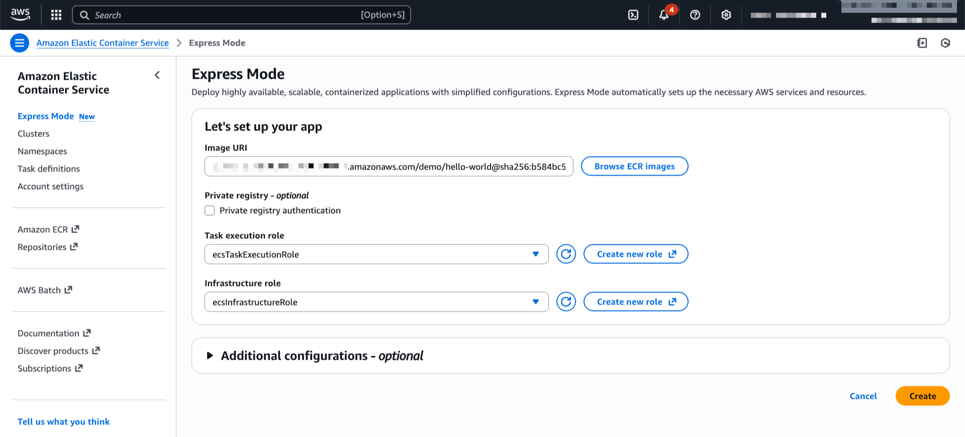
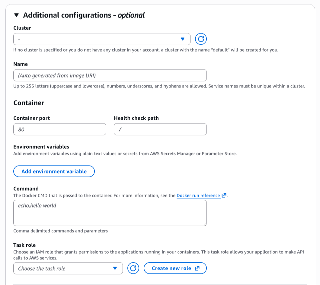
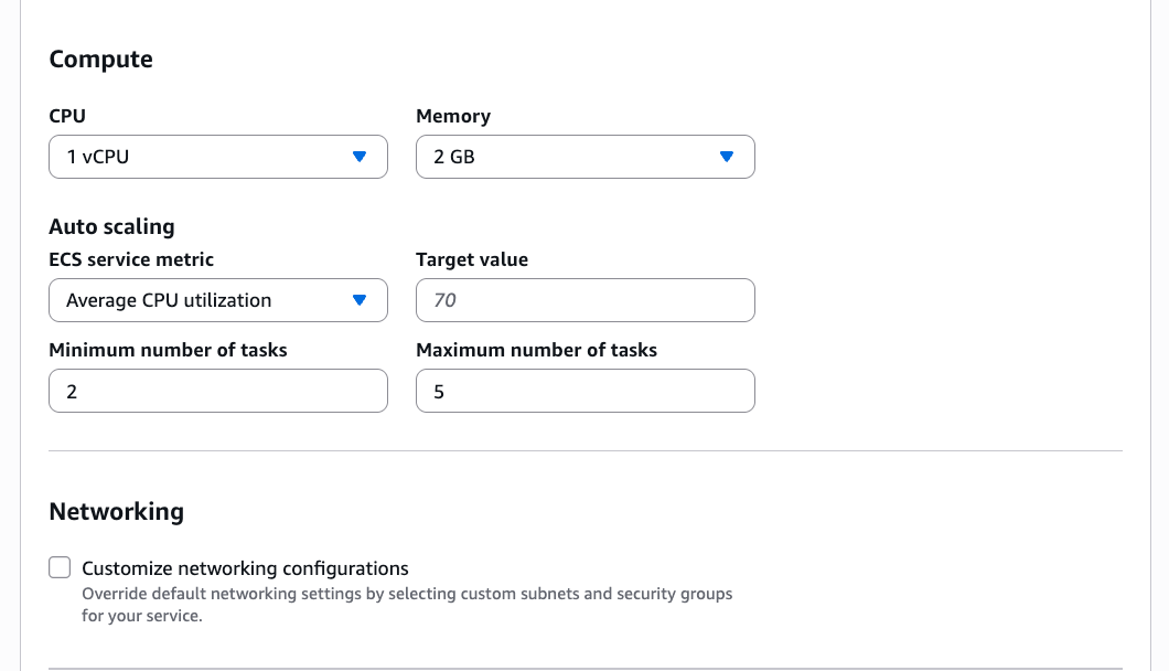
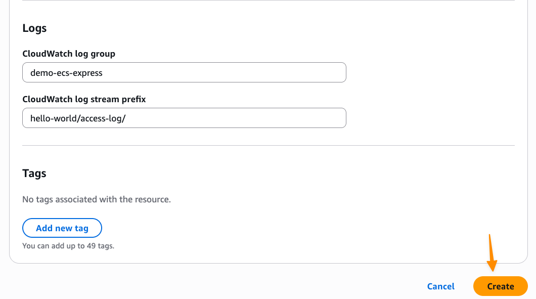
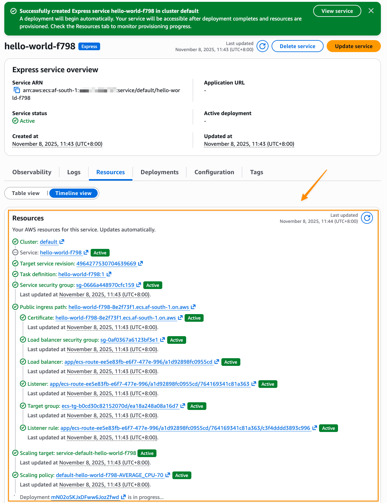
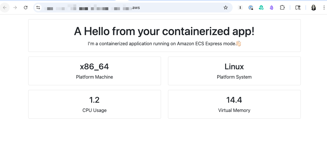
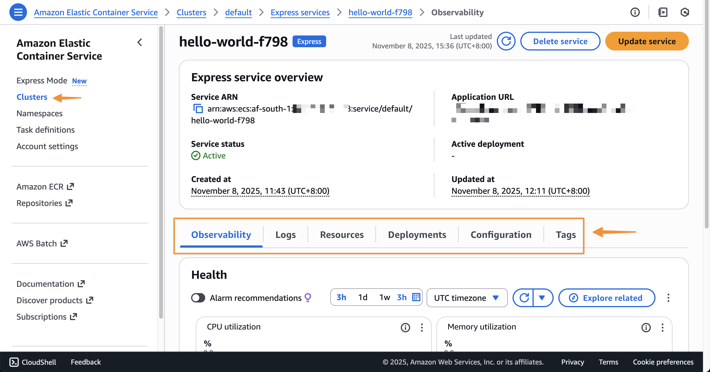
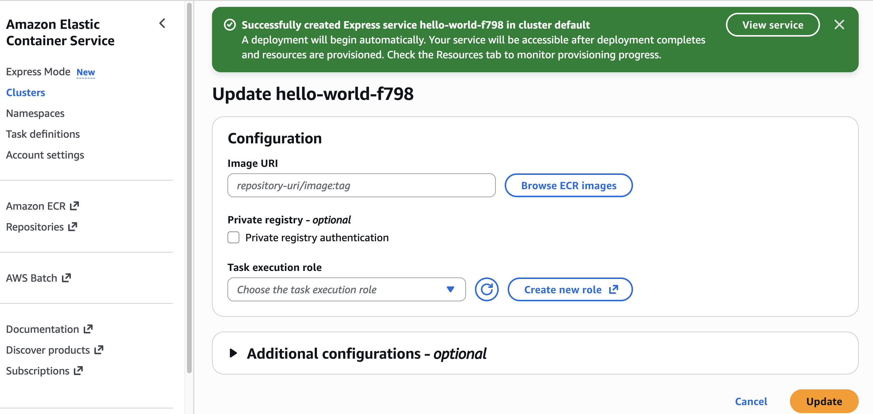


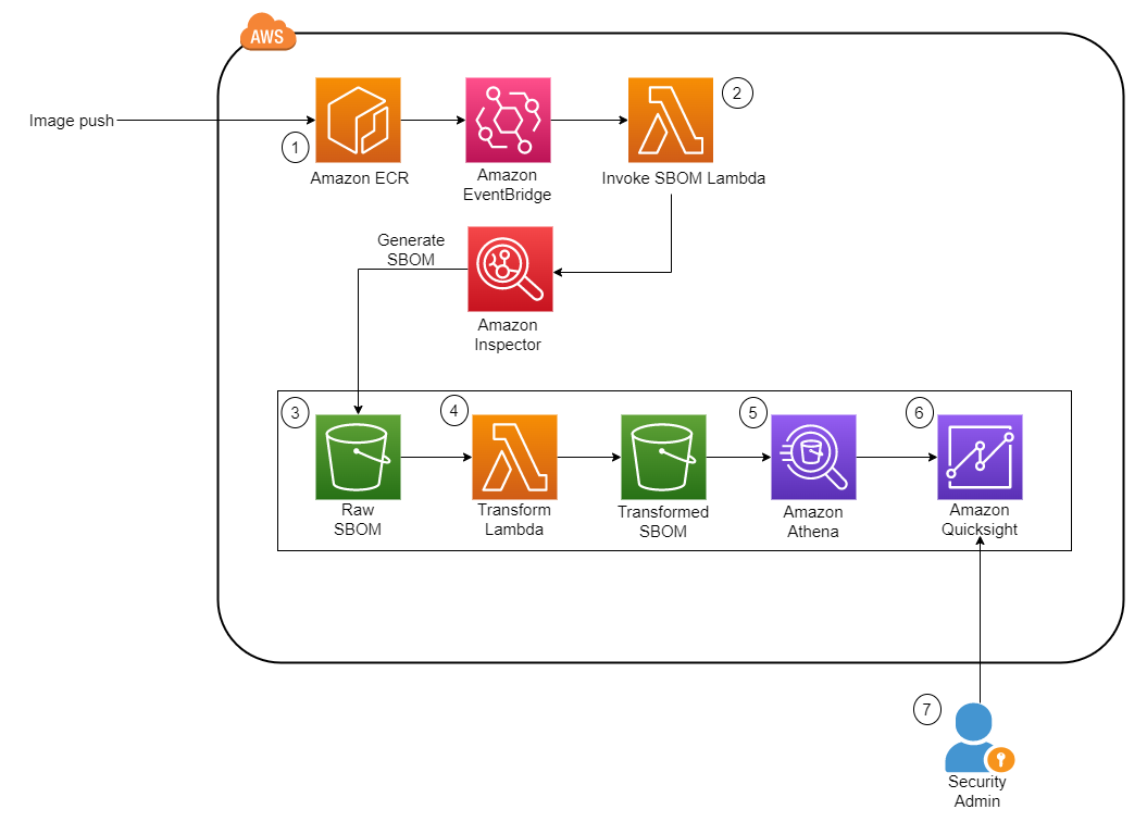
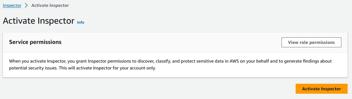


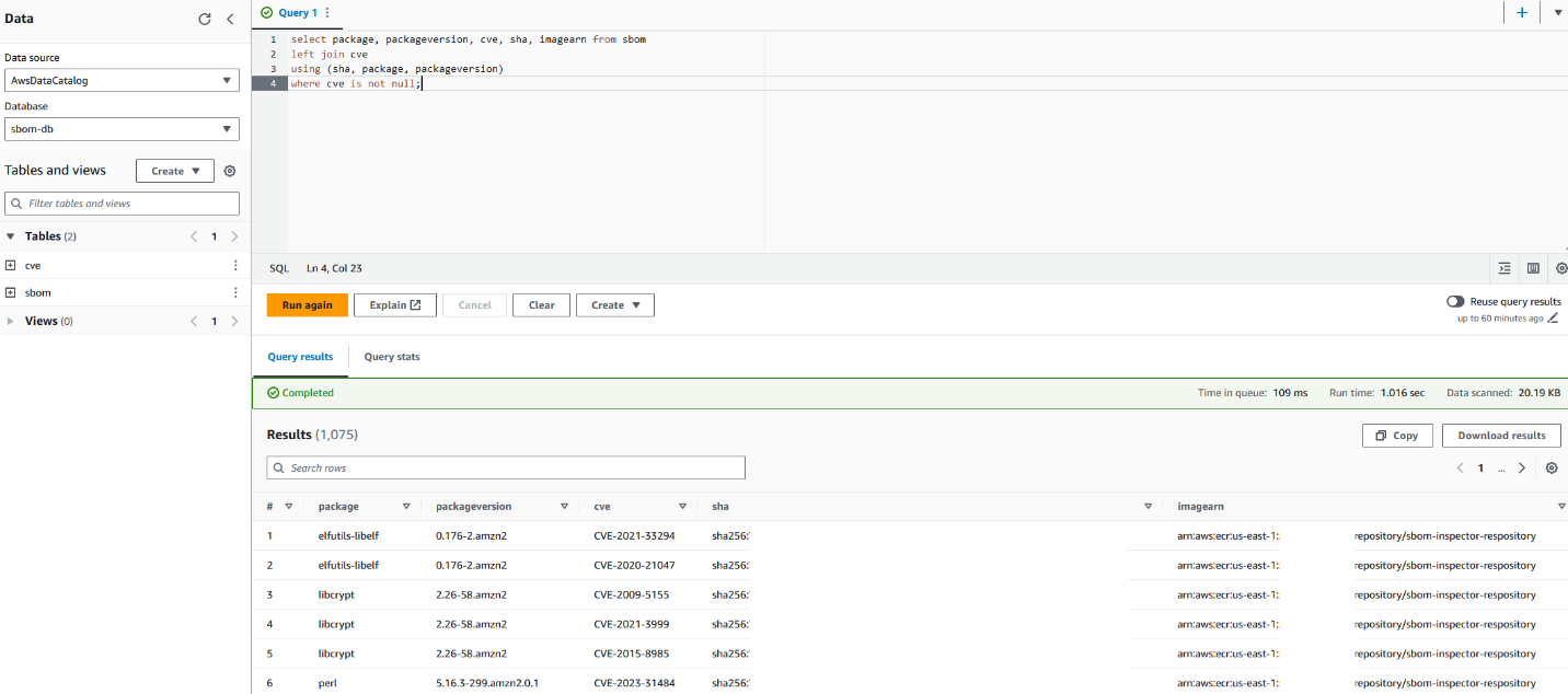

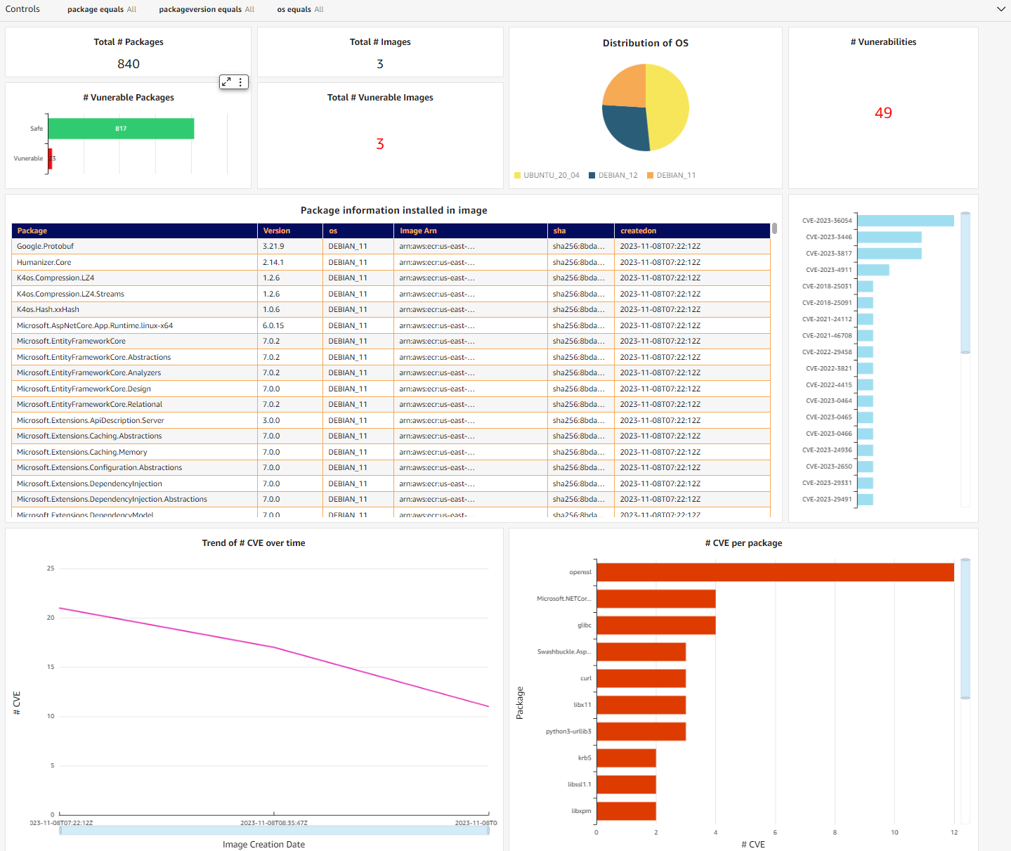
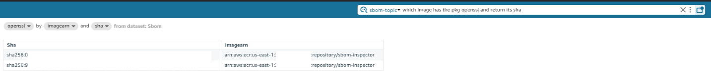


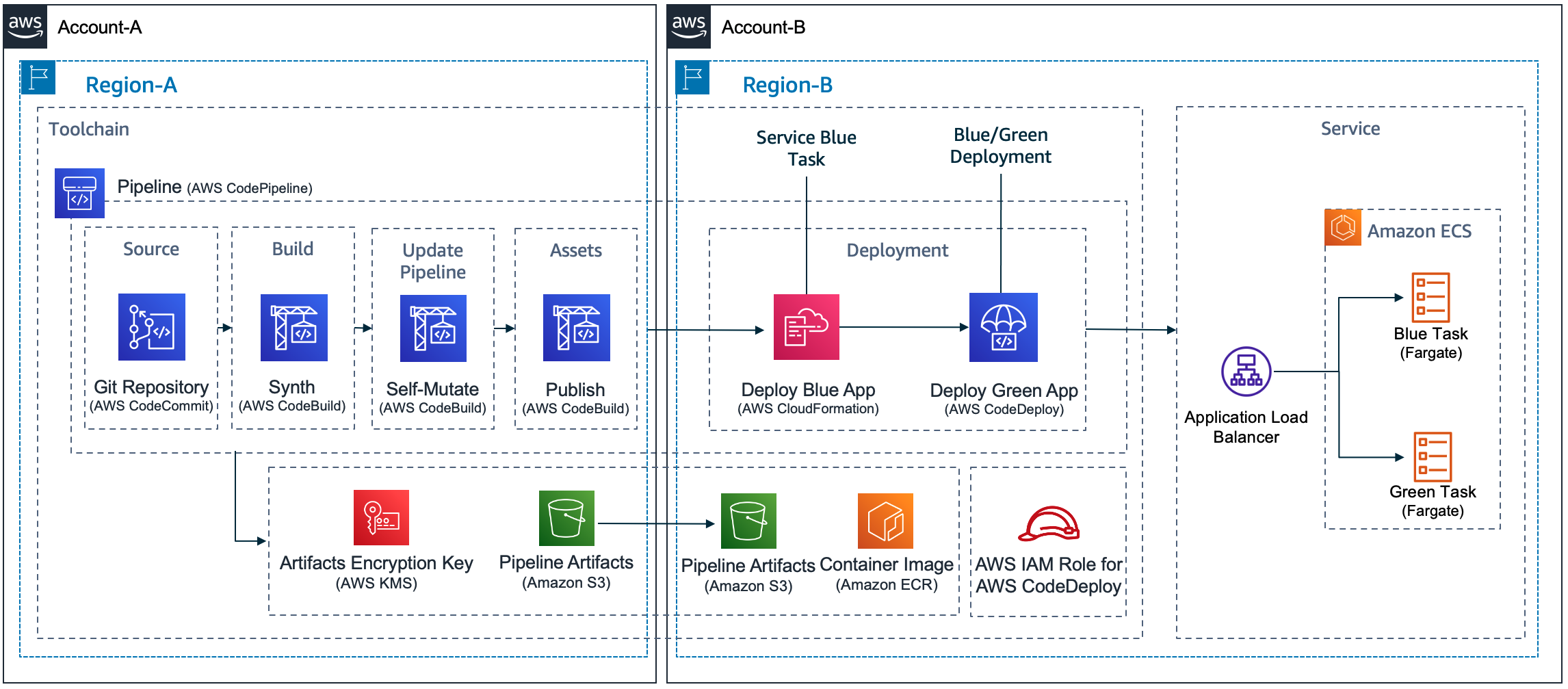


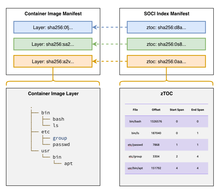


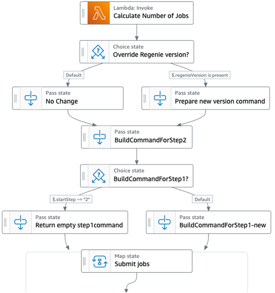
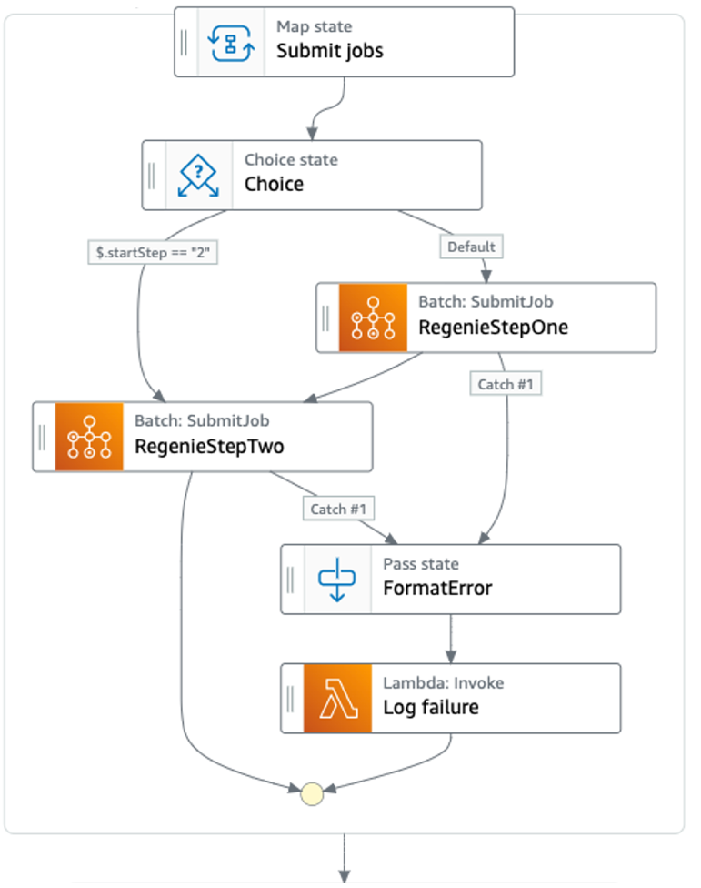


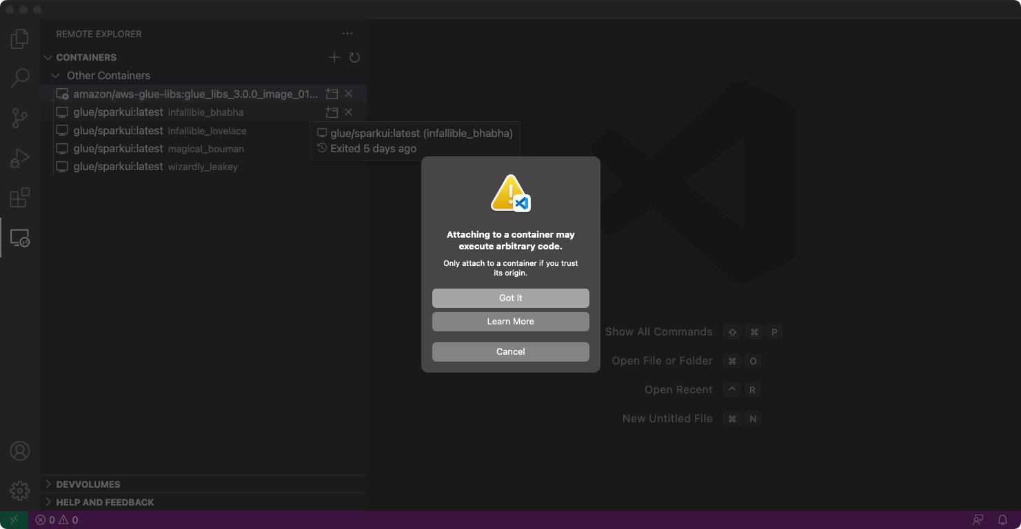
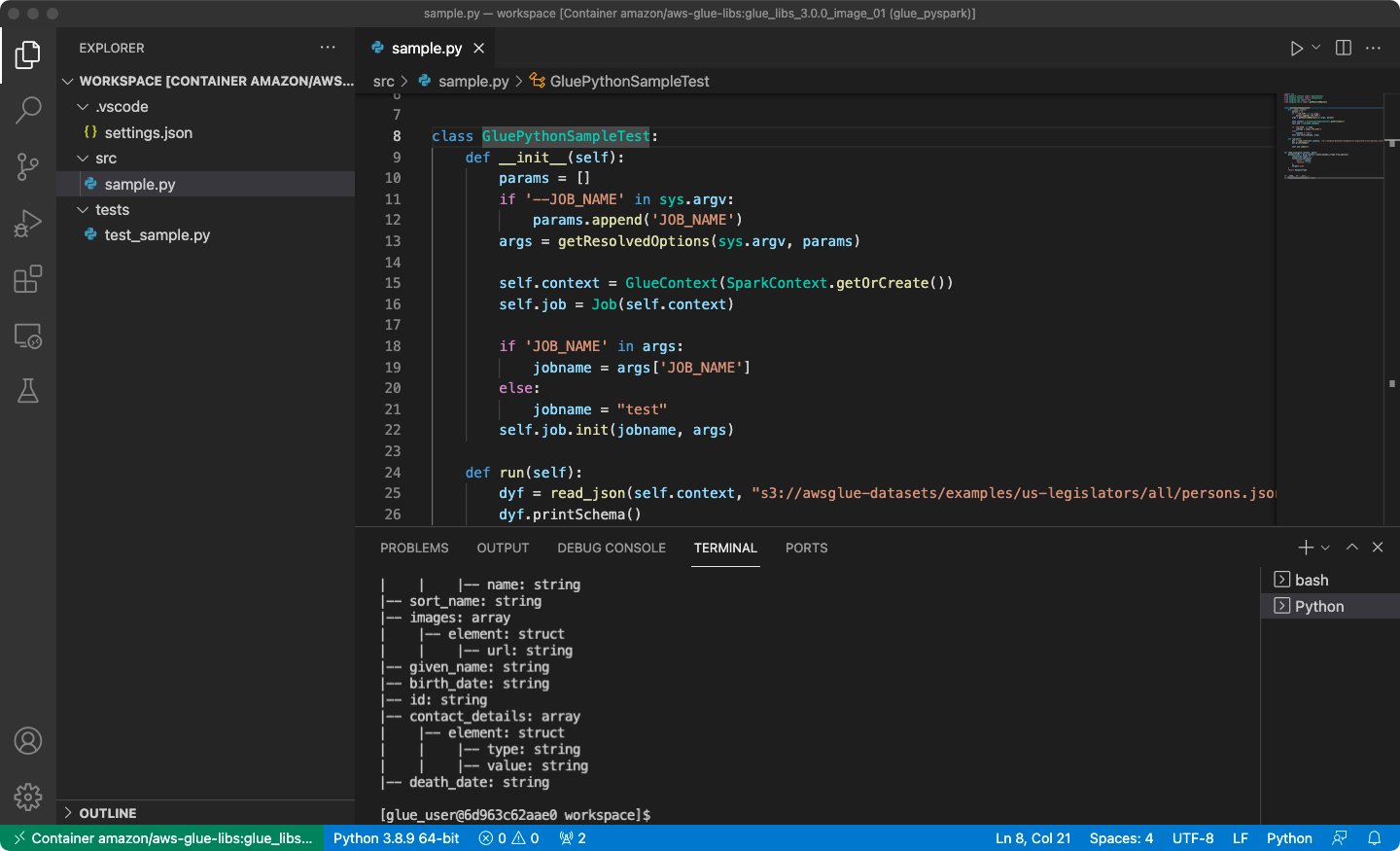


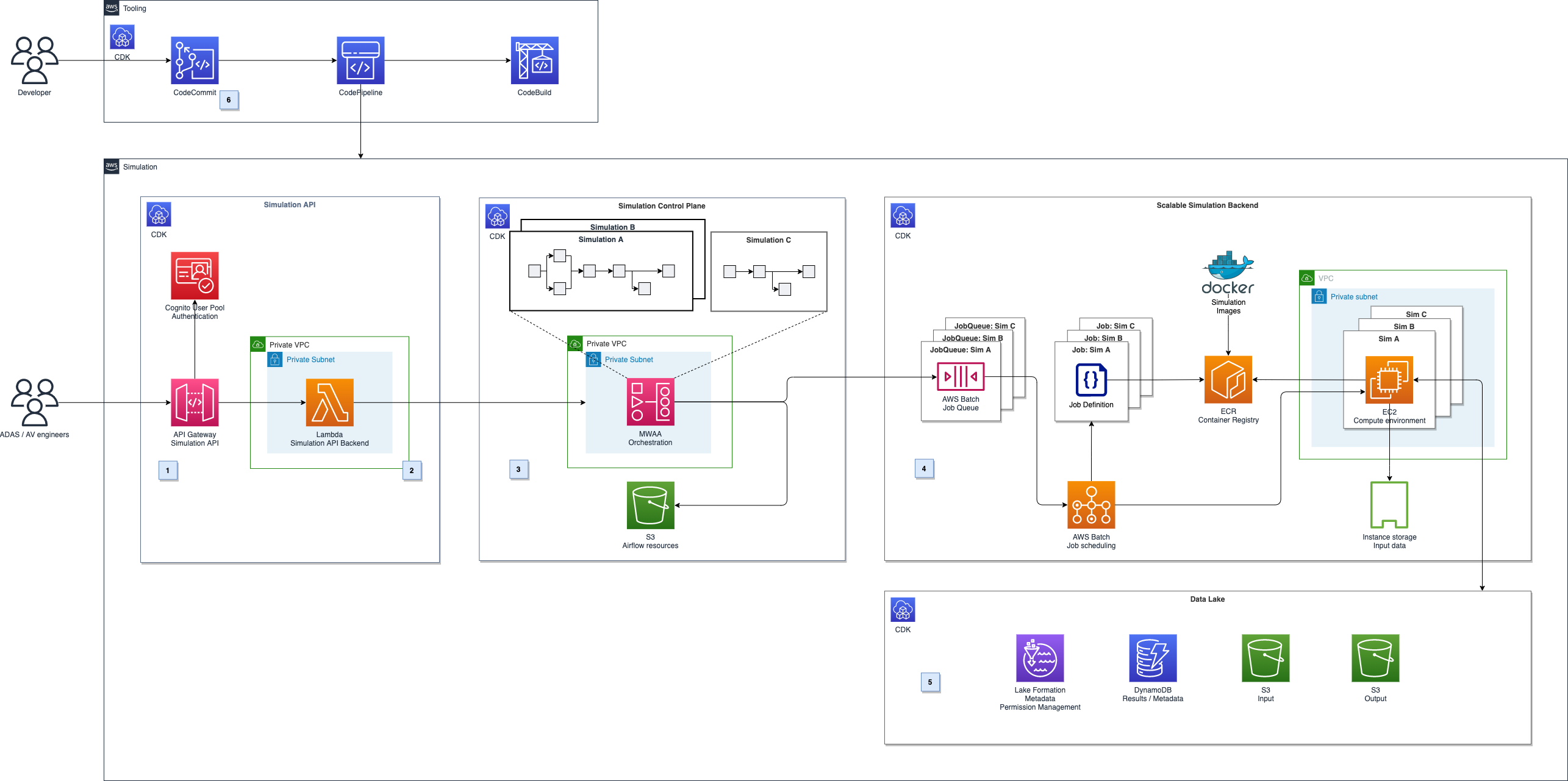
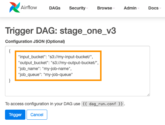
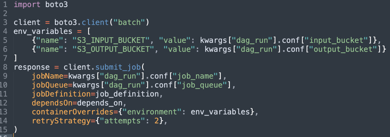
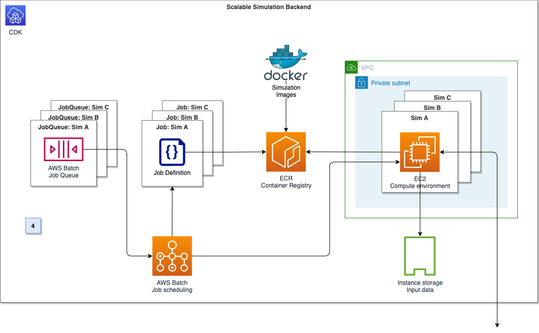
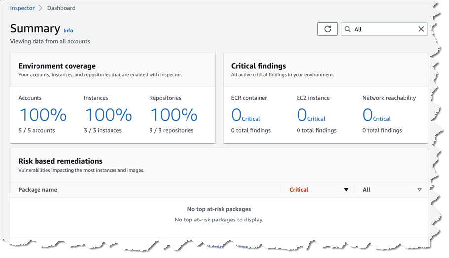
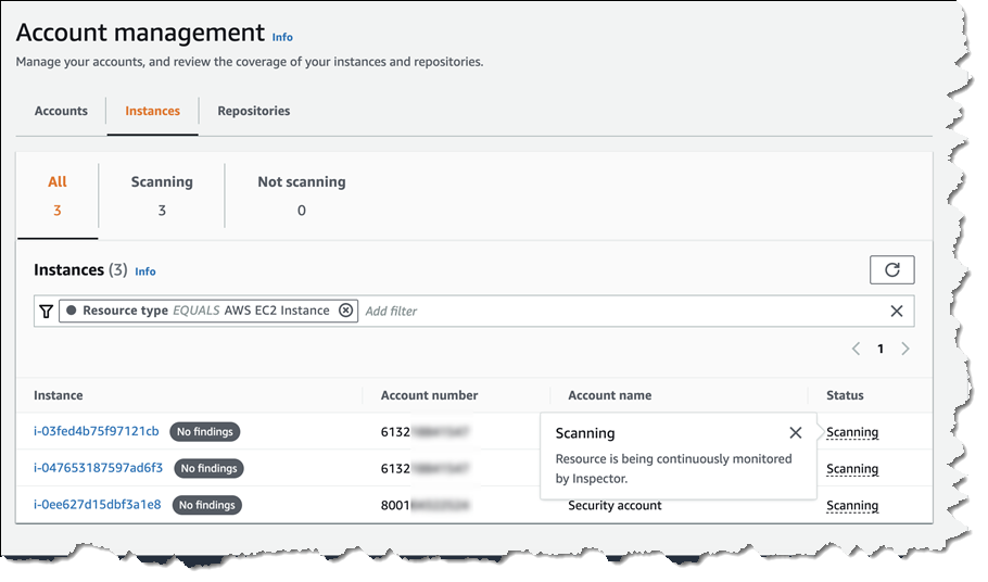

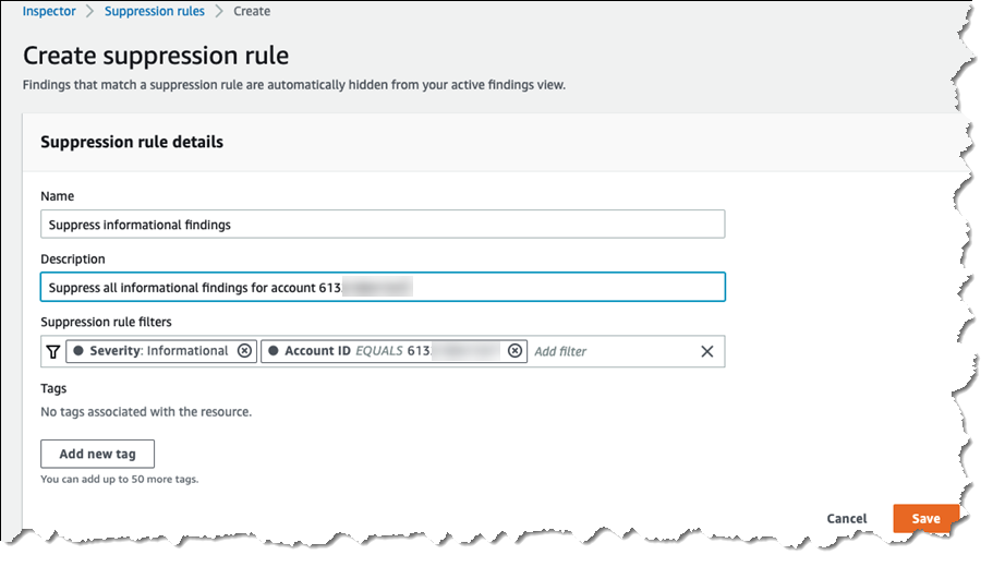
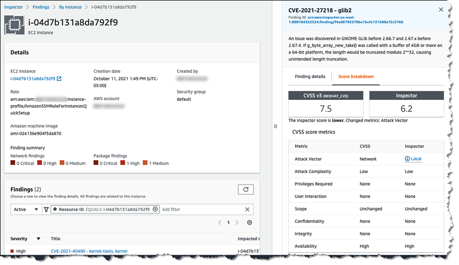

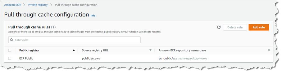


