Post Syndicated from The Atlantic original https://www.youtube.com/watch?v=2c85x4YGSec
A Conversation With Whitney Wolfe Herd
Post Syndicated from The Atlantic original https://www.youtube.com/watch?v=hoQ_wkclpSA
Conversations With Rob Bonta, John Formella, and David Sunday
Post Syndicated from The Atlantic original https://www.youtube.com/watch?v=CoKia8W3Yoc
Run open weight models on AWS Bedrock in AWS European Sovereign Cloud
Post Syndicated from Marta Taggart original https://aws.amazon.com/blogs/security/run-open-weight-models-on-aws-bedrock-in-aws-european-sovereign-cloud/
European organizations can run AI workloads on Amazon Web Services (AWS) while keeping data within the European Union (EU) and meeting regulatory requirements. You can now run generative AI workloads on open weight models on Amazon Bedrock in the AWS European Sovereign Cloud. We’re excited to announce the general availability of the first open weight model family, Gemma 4, on the Amazon Bedrock next-generation inference engine in the AWS European Sovereign Cloud. Gemma 4, released under the Apache 2.0 license, on Amazon Bedrock benefits from the same data residency and operational controls that define the AWS European Sovereign Cloud so you can build, iterate, and scale generative AI applications while meeting digital sovereignty requirements.
The AWS European Sovereign Cloud is an independent cloud for Europe, located entirely within the EU, designed to help customers meet their most stringent digital sovereignty requirements. It runs entirely within the EU and is independently operated with strong technical controls, sovereign assurances and legal protections. Only AWS employees who reside in the EU control day-to-day operations, including access to data centers, technical support, and customer service.
In this post, we explain how the Amazon Bedrock inference engine protects your inference data when running Gemma 4 models, how the AWS European Sovereign Cloud keeps it within the EU, and then walk through the available Gemma 4 models and your first inference request.
Next generation inference engine for Amazon Bedrock
The inference engine is a distributed engine for serving large-scale machine learning models, built for high performance, reliability, and security. You reach it through the bedrock-mantle endpoint, which supports OpenAI-compatible APIs (the Responses and Chat Completions APIs). You can bring an existing OpenAI SDK codebase to Amazon Bedrock by changing only the base URL and API key. The Responses API supports stateful conversation management, which rebuilds context without you passing conversation history with each request. Stored responses are scoped by Amazon Bedrock project, a logical boundary that represents a workload for access control, cost tracking, and usage monitoring.
The engine applies the same operational security practices you rely on across AWS. Access follows a least privilege model, where each operator has access only to the systems a specific task requires, and only for the time that privilege is needed. Any access to systems that store or process customer data or metadata is logged, monitored for anomalies, and audited. All your prompts and responses are kept private during inference.
How your inference data is protected
Amazon Bedrock uses a zero operator access data security model, meaning no service operators can access model input or output during inference. It also uses a zero data retention model, so by default it doesn’t store your inputs or outputs. For certain models, limited retention might apply for abuse detection (see the Amazon Bedrock abuse detection documentation). Your prompts and responses are encrypted in transit and, by default, are not shared with the model provider.
All inference stays within the eusc-de-east-1 AWS Region as described in the following section on data residency. Combined with the data residency and EU-based operations of the AWS European Sovereign Cloud, this gives organizations in highly regulated industries the confidence to run their most sensitive AI workloads in the cloud.
Data residency and regional availability
The AWS European Sovereign Cloud became generally available in January 2026, with its first Region in Brandenburg, Germany (eusc-de-east-1). It’s a separate, independently operated cloud, with infrastructure located entirely within the EU and no critical dependencies on non-EU personnel or infrastructure. All your content remains within the Region you select unless you choose otherwise. Beyond content, customer-created metadata including roles, permissions, resource labels, and configurations also stays within the EU. The AWS European Sovereign Cloud is operated exclusively by EU residents located in the EU. We’re also gradually transitioning the AWS European Sovereign Cloud to be operated exclusively by EU citizens located in the EU. During this transition period we will continue to work with a blended team of EU residents and EU citizens located in the EU.
All Amazon Bedrock inference requests, including Gemma 4, use in-Region inference in eusc-de-east-1, which keeps every request within the AWS European Sovereign Cloud. Global cross-Region inference, which routes requests across commercial AWS Regions worldwide, isn’t available in the AWS European Sovereign Cloud.
Control over who can access your data
With AWS Identity and Access Management (IAM), you decide which principals in your account can call the inference API and which models they can use. Fine-grained permissions let you grant only the access each workload needs, following least privilege, and we recommend short-lived credentials over long-term keys.
For auditing, every call to the endpoint is recorded in AWS CloudTrail, giving your security and compliance teams an audit trail of who invoked inference and when. You can also monitor usage with Amazon CloudWatch and set alarms on patterns that matter to you, such as unexpected spikes in request volume.
Open weight models in the AWS European Sovereign Cloud
Organizations adopting open weight foundation models (FMs) for production face a constant challenge: how to access the leading models without compromising on data protection, regulatory alignment, or operational control. Amazon Bedrock removes that challenge. It gives you leading open weight FMs through a fully managed service, with inference running entirely on infrastructure operated by AWS and the security and privacy controls you expect from Amazon Bedrock. Because the models are open weight, you can independently evaluate the model architecture and training methodology, benchmark your own workloads, and fine-tune on proprietary data when customization is required.
Gemma 4 is a family of open weight models, released under the Apache 2.0 license. It’s available in three instruction-tuned variants, so you can evaluate and choose the model that fits your workload. The following table provides guidance on which model to choose based on your use case:
|
Model |
Use case |
Specifications |
|
Gemma 4 31B |
Reasoning-heavy or coding-heavy with a single dense model |
30.7 billion parameter dense model with a 256 K token context window |
|
Gemma 4 26B-A4B |
Cost-sensitive at high throughput, with knowledge breadth requirements |
Mixture-of-experts model with 25.2 billion total parameters and 3.8 billion active per token, with a 256 K token context window |
|
Gemma 4 E2B
|
Latency-sensitive, on-device-style, or multimodal classification |
Compact model with 5.1 billion total parameters and 2.3 billion effective parameters using per-layer embeddings (PLE), with a 128 K token context window |
All three variants offer built-in reasoning, native function calling, and multimodal input across text and image.
Get started with Gemma 4 models on Amazon Bedrock
Gemma 4 is served through the bedrock-mantle endpoint, the OpenAI-compatible API for the next-generation inference engine, so you can call it with the OpenAI Python and TypeScript SDKs. Use the following steps to use the OpenAI Python SDK to send your first request to Gemma 4 31B in the AWS European Sovereign Cloud.
Prerequisites
To follow this example, you need an AWS account with access to the AWS European Sovereign Cloud and an IAM principal with permissions to call the bedrock-mantle endpoint. Create an IAM policy that grants the two actions this walkthrough uses, then attach it to your IAM principal. The bedrock-mantle:CreateInference action runs inference, and the bedrock-mantle:CallWithBearerToken action authenticates with an Amazon Bedrock API key. The following sample policy grants the actions this example needs. Scope the resources further for your environment as described after the policy.
Replace <account-id> and <project-id> with your own values.
Install the OpenAI SDK and the Amazon Bedrock token generator with the command pip install “openai>=2.45.0" aws-bedrock-token-generator.
Authenticate
You authenticate with an Amazon Bedrock API key. Amazon Bedrock offers two types of API keys. Short-term keys expire automatically within 12 hours and inherit the permissions of the IAM principal that generated them, which makes them the recommended choice for production. Long-term keys last until a configured expiration and are intended for development and exploration. For production, use the auto-refreshing short-term key shown in the following example, or store the key in AWS Secrets Manager.
Alternatively, you can pass a short-term API key through an environment variable. This key isn’t refreshed and expires after at most 12 hours.
Run your first inference with the Responses API
The Responses API uses a single input field and returns the generated text in output_text. Setting store to false means Amazon Bedrock doesn’t retain the request or response.
Call the Chat Completions API
You can also call the OpenAI-compatible Chat Completions endpoint directly. If you use AWS credentials instead of an API key, sign the request with AWS Signature Version 4 (SigV4), as in the following example.
Clean up
This walkthrough creates no persistent resources, so there’s nothing to delete. The short-term API keys used here expire automatically within 12 hours.
Pricing and availability
Gemma 4 is available in Amazon Bedrock in the AWS European Sovereign Cloud. You pay per token with no upfront commitment, and usage counts toward your existing AWS commitments. For current pricing, see Amazon Bedrock pricing. For model and Regional availability, see Regional availability by models.
Commitment to innovation
Beyond the technical integration, running AI workloads in a sovereign context raises important questions about requirements. As you plan AI workloads for a sovereign context, evaluate them against your organization’s requirements for data residency, model governance, and operational control. The AWS European Sovereign Cloud is designed to help you meet these requirements in the EU.
AWS is committed to making AWS the best place for European organizations to innovate with AI, without compromise. To learn more about AWS European Sovereign Cloud visit aws.eu.
If you have feedback about this post, submit comments in the Comments section below.
Padma Lakshmi Recommends Five Spices to Keep in Your Kitchen
Post Syndicated from The Atlantic original https://www.youtube.com/shorts/deb2PNXYj5o
A Conversation With Rahm Emanuel
Post Syndicated from The Atlantic original https://www.youtube.com/watch?v=LG6_Rtil_mo
New low-cost burstable Amazon EC2 T8i instances are generally available
Post Syndicated from Channy Yun (윤석찬) original https://aws.amazon.com/blogs/aws/new-low-cost-burstable-amazon-ec2-t8i-instances-are-generally-available/
Today, we’re announcing the general availability of new low-cost burstable Amazon EC2 T8i instances powered by custom sixth generation Intel Xeon Scalable Processors (Granite Rapids), available only on AWS. T8i instances are among the lowest-cost EC2 instances and deliver up to 30% better price performance over previous generation T3 instances. These instances are designed to run a variety of low-to-moderate CPU utilization workloads such as freemium services, training and demo environments, staging and development, data processing, microservices, low-traffic websites, and login gateways.
T8i instances
Thousands and thousands of customers run various lightweight workloads on T3 instances that require small, cost-effective compute configurations. These include microservices architectures, low-traffic websites, development and testing environments, small databases, data processing jobs, and short-duration compute tasks. Many of these customers like T family’s burstable performance model, which provides a baseline level of CPU performance with the ability to burst above the baseline when needed using CPU credits.
As customers modernize their infrastructure, migrate from on-premises environments, adopt event-driven and microservices architectures, and experiment with AI inference workloads, they have asked for newer generation cost-optimized small instances, better price performance to reduce their total cost of ownership, and a seamless migration path that leverages their existing knowledge and tooling.
T8i instances address each of these requests:
- Up to 30% better price performance. Powered by the AWS Nitro System and custom sixth generation Intel Xeon Scalable Processors (Granite Rapids), T8i instances enable customers to lower their total cost of ownership with up to 30% better price performance.
- Up to 70% higher compute performance. T8i instances deliver up to 70% higher compute performance, up to 1.25x higher network bandwidth, and up to 2.4x higher EBS bandwidth compared to T3 instances.
- Seamless upgrade from T3. For existing T3 customers, upgrading to T8i is straightforward. The instances offer the same CPU credit system and the same familiar lightweight compute options customers already know. Customers simply select T8i instead of T3 and immediately benefit from improved price performance.
- Cost-effective entry point for new customers. For customers new to AWS or migrating from on-premises, T8i instances provide one of the most cost-effective entry points to run workloads that need low-to-moderate CPU utilization or for running short-duration compute tasks such as batch processing, event-driven functions, or CI/CD pipelines.
Instance specifications
T8i instances offer four sizes, each with two vCPU offered as a single core. The following table summarizes the specifications.
| Instance size | vCPUs | Memory (GiB) | Baseline Performance /vCPU (%) | CPU credits earned / hour | Network burst bandwidth (Gbps) |
| t8i.nano | 2 | 0.25 | 5 | 3 | Up to 6.25 |
| t8i.micro | 2 | 0.5 | 10 | 6 | Up to 6.25 |
| t8i.small | 2 | 1 | 20 | 12 | Up to 6.25 |
| t8i.medium | 2 | 2 | 20 | 12 | Up to 6.25 |
Like T3, T8i instances offer unique vCPU-to-memory ratios such as 1:0.25, 1:0.5, and 1:1 that are not offered by other EC2 instances. Like T3, T8i instances utilize the CPU credit system along with the Standard and Unlimited credit configuration modes. Unlimited mode is the default on T8i.
For workloads that need larger instance sizes above T8i offerings (nano, micro, small, and medium), I recommend M8i Flex instances that offer up to 30% better price performance than equivalent previous generation T3 instances along with the flexibility to scale up to 16xlarge.
Now available
Amazon EC2 T8i instances are available today in the following AWS Regions: US East (N. Virginia, Ohio), US West (Oregon, N. California), Asia Pacific (Hyderabad, Malaysia, Mumbai, Seoul, Singapore, Sydney, Tokyo), Canada (Central), and Europe (Frankfurt, Ireland, London, Paris). For Regional availability and upcoming Region expansion, search the instance type in the CloudFormation resources tab of AWS Capabilities by Region.
You can purchase T8i instances via On-Demand instances, and Spot instances with Savings Plan option coming soon. T8i instances support shared tenancy only and do not support Dedicated tenancy or Dedicated Hosts. t8i.micro and t8i.small instances are also available under the AWS Free Tier. To learn more, visit the Amazon EC2 Pricing page.
Try T8i instances in the Amazon EC2 console and send feedback to AWS re:Post for EC2 or through your usual AWS Support contacts.
— Channy
Pete Buttigieg Declares That We Need to “Get a Better Congress”
Post Syndicated from The Atlantic original https://www.youtube.com/shorts/vzP0yUCND3c
A Conversation With Malcolm Gladwell
Post Syndicated from The Atlantic original https://www.youtube.com/watch?v=3vfKZF4kw_A
A Conversation With Ben McKenzie
Post Syndicated from The Atlantic original https://www.youtube.com/watch?v=9MUGEw1Vt_M
AWS Elastic Beanstalk introduces Cluster Mode
Post Syndicated from Channy Yun (윤석찬) original https://aws.amazon.com/blogs/aws/aws-elastic-beanstalk-introduces-cluster-mode/
Since the first launch of AWS Elastic Beanstalk in 2011, customers have deployed full-stack applications in Java, .NET, Python, Node.js, PHP, Ruby, and Go, trusting Elastic Beanstalk to manage deployment and infrastructure operations so they could focus on business logic. Fifteen years later, that trust has only deepened, and the service has been rebuilt to match it. Now, AWS Elastic Beanstalk is the application management service on AWS that takes full operational responsibility for your production environments. Bring applications however they exist today: source code, Dockerfiles, or container images. Elastic Beanstalk creates and manages the production environment underneath. You manage your application. AWS manages everything else, deploying, scaling, patching, monitoring, and maintaining it continuously. That operational responsibility stays with AWS, for the life of the application.
We have been rebuilding the operational engine underneath and delivering a series of capabilities that make it more powerful than ever. Elastic Beanstalk now uses AI-powered environment analysis to diagnose health issues and recommend fixes automatically. A new official GitHub Action lets teams deploy directly from their existing CI/CD workflows with a single YAML configuration. And we rebuilt the infrastructure foundation to deliver OpenTelemetry-based observability, traffic-splitting deployments with automatic rollback, event-driven autoscaling, secrets management through AWS Secrets Manager, and HTTPS by default via AWS Certificate Manager.
Today, we’re announcing the next chapter of AWS Elastic Beanstalk: a new fully-managed Cluster Mode that deploys, scales, patches, monitors, and upgrades your applications continuously for the life of the workload. You bring your application. AWS runs it.
A new Cluster Mode is built for teams running a portfolio of applications. Instead of operating each application in isolation, you run multiple applications that share infrastructure powered by Amazon Elastic Kubernetes Service (Amazon EKS), fully managed with a single operational baseline. Multiple applications share resources, so per-application cost decreases as your portfolio grows without adding operational complexity. Whether you run ten applications or a hundred, you manage them through one experience, with the same operational guarantees across every stack.
Elastic Beanstalk Cluster Mode benefits for your workloads:
- Source code to production, any runtime. Upload source code in Java, .NET, Python, Node.js, PHP, Ruby, or Go. Elastic Beanstalk handles containerization automatically through Cloud Native Buildpacks when needed. No Dockerfile and no rearchitecting required. You can bring legacy applications from on-premises or deploy new services in any supported language.
- Enterprise compliance built in. Elastic Beanstalk is HIPAA eligible, PCI DSS compliant, and aligned to SOC 1/2/3 with no additional configuration, so teams in regulated industries can deploy production workloads with the compliance posture they already require.
- Production-grade deployment strategies. All-at-once, rolling, immutable, and traffic-splitting deployments with automatic rollback on failure. Event-driven autoscaling. AWS Secrets Manager integration. All native OpenTelemetry enabling easy integration with most observability backends, including Amazon CloudWatch.
- AI-powered troubleshooting. When something goes wrong, Elastic Beanstalk collects service-side logs and provides AI-generated recommendations to help you resolve issues faster without digging through infrastructure.
A first look of Elastic Beanstalk Cluster Mode
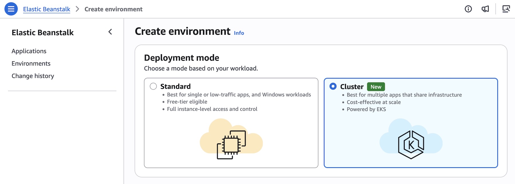
To get started, go to the Elastic Beanstalk console, create a new environment, and choose the Cluster in the Deployment type.
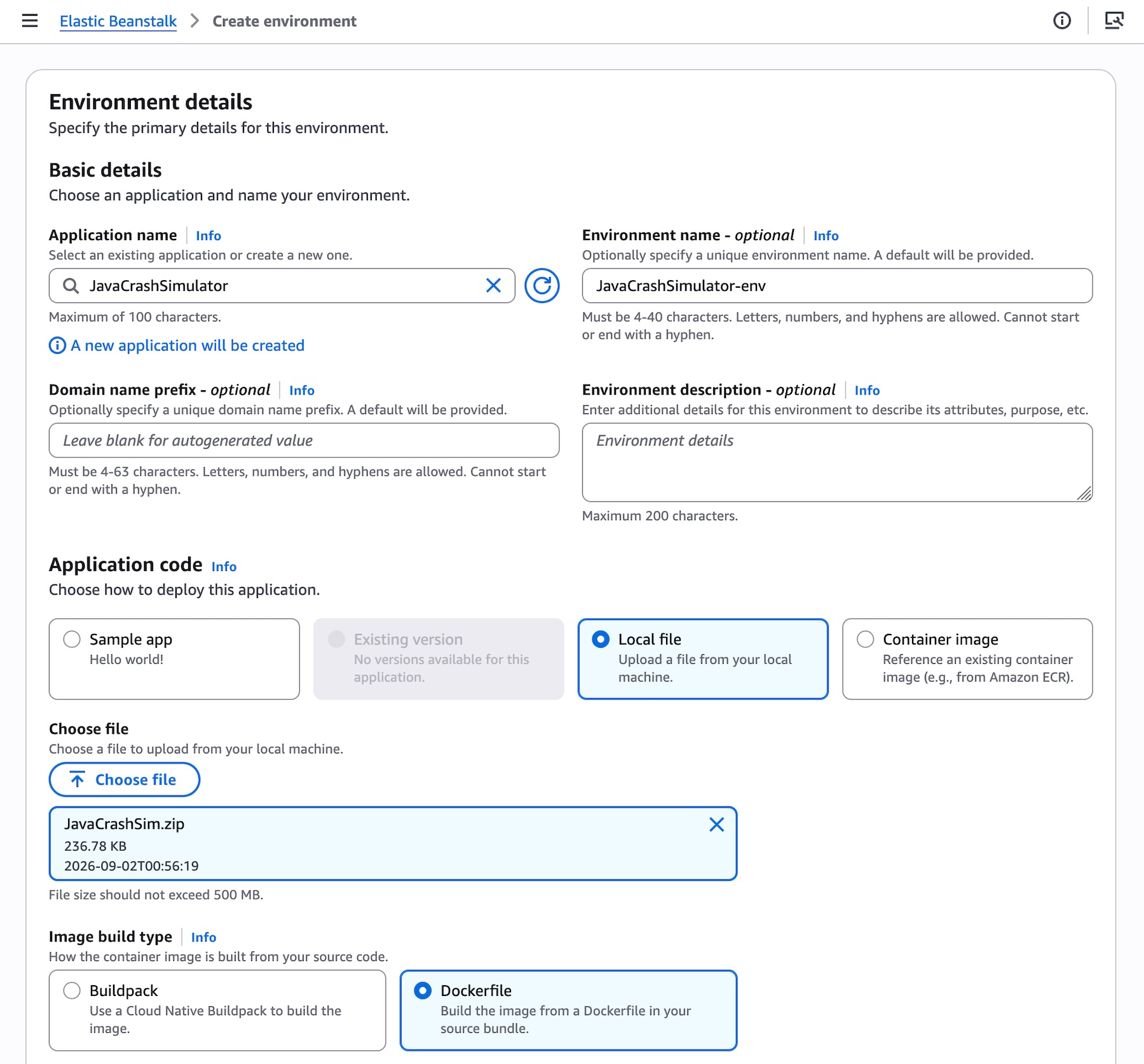
Elastic Beanstalk accepts source code, docker file, or container image to deploy your application. For example, you can provide the application code for your environment by selecting Local file and specifying container image build options. For the rest of the sections, the default values should be good for most scenarios.
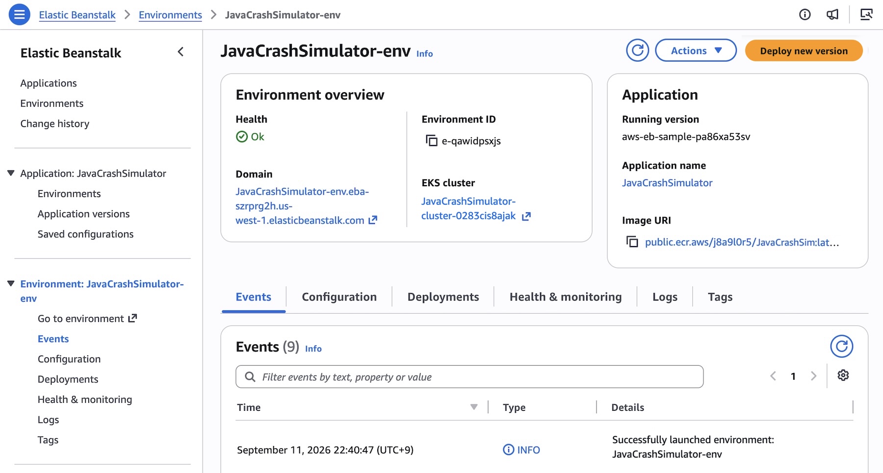
Choose Create button and the deployment will begin! Note that the first deployment for a given set of subnets triggers EKS cluster creation, which takes about ten-ish minutes. Subsequent deployments are faster because they reuse an existing EKS cluster.
Here’s what it looks like when deployment is successful:
You can also use AWS Command Line Interface (AWS CLI), the EB CLI, or AWS SDKs. For example, consider deploying an application made up of several microservices to Kubernetes. Create an application first.
aws elasticbeanstalk create-application \
    --application-name "my-microservice" \
    --description "Multi-services demo" \
Each microservice may have pre-built images in Amazon Elastic Container Registry (Amazon ECR). Register them as application versions:
IMAGES=(
    "frontend-v1|public.ecr.aws/my-microservices/frontend:v1"
    "cartservice-v1|public.ecr.aws/my-microservices/cart:v1"
    "paymentservice-v1|public.ecr.aws/my-microservices/payment:v1"
    "shippingservice-v1|public.ecr.aws/my-microservices/shipping:v1"
)

for entry in "${IMAGES[@]}"; do
    IFS='|' read -r label uri <<< "$entry"
    aws elasticbeanstalk create-application-version \
        --application-name $APP_NAME \
        --version-label "$label" \
        --image-configuration Source="{Uri=$uri}" \
	--region "us-west-2
    echo "Registered: $label"
done
You can set and deploy the corresponding service options for each service. For example, the frontend service is the only service that needs a public internet interface such as Application Load Balancer and also sets a health check path since it’s an HTTP service:
[
    {"Namespace": "aws:elasticbeanstalk:eks", "OptionName": "cluster-role", "Value": "arn:aws:iam::0123456789012:rol<...>"},
    {"Namespace": "aws:elasticbeanstalk:eks", "OptionName": "node-role", "Value": "arn:aws:iam::0123456789012:role/E<...>"},
    {"Namespace": "aws:elasticbeanstalk:eks:environment", "OptionName": "observability-role", "Value": "arn:aws:iam::0123456<...>"},
    {"Namespace": "aws:elasticbeanstalk:eks:environment", "OptionName": "subnets", "Value": "subnet-1,subnet-2,subnet-3,<...>"},
    {"Namespace": "aws:elasticbeanstalk:eks:environment:autoscaling", "OptionName": "min-replica", "Value": "1"},
    {"Namespace": "aws:elasticbeanstalk:eks:environment:autoscaling", "OptionName": "max-replica", "Value": "2"},
    {"Namespace": "aws:elasticbeanstalk:eks:environment", "OptionName": "cpu", "Value": "0.5"},
    {"Namespace": "aws:elasticbeanstalk:eks:environment", "OptionName": "memory", "Value": "256Mi"},
    {"Namespace": "aws:elasticbeanstalk:eks:environment", "OptionName": "memory-limit", "Value": "512Mi"},
    {"Namespace": "aws:elasticbeanstalk:eks:environment", "OptionName": "service-port", "Value": "8080"},
    {"Namespace": "aws:elasticbeanstalk:eks:alb", "OptionName": "scheme", "Value": "internet-facing"},
    {"Namespace": "aws:elasticbeanstalk:eks:alb", "OptionName": "healthcheck-path", "Value": "/_healthz"}
] #frontend-options.json namespaces
Now, create the frontend service environment with these options. You can continue to deploy each service environment in a similar manner.
aws elasticbeanstalk create-environment \
    --application-name my-microservice \
    --environment-name frontend \
    --version-label frontend-v1 \
    --tier Name=Cluster,Type=EKS \
    --option-settings file:///tmp/frontend-options.json \
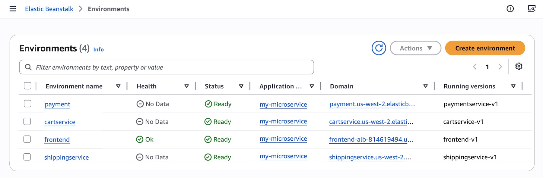
Here’s a look at the console once all services are deployed:
Elastic Beanstalk Standard powered by Amazon Elastic Compute Cloud (EC2) continues to be fully supported. Standard and Cluster Mode environments run side by side within the same Elastic Beanstalk application, enabling teams to migrate one environment at a time at their own pace. Validation checks confirm compatibility before any changes are made, so no environment is forced to move.
Elastic Beanstalk Standard Mode remains the best fit for:
- Single applications or single-environment use cases
- Windows/.NET Framework workloads on IIS
- Applications that cannot be containerized
- Workloads spending under $500/month where the EKS control plane fee and EKS Auto Mode premium add overhead that a single application cannot offset through bin-packing
To learn more about how to deploy and manage your applications in the Cluster Mode, visit the Elastic Beanstalk Cluster Mode documentation.
Now available
AWS Elastic Beanstalk Cluster Mode is generally available today in all AWS Regions that Elastic Beanstalk is available. For Regional availability and a future roadmap, visit the AWS Capabilities by Region. If you want to call APIs, search documentation, find regional availability, and troubleshooting about this new feature, try using the AWS MCP Server and plugins with your preferred AI tool.
There is no additional charge for Elastic Beanstalk Cluster Mode. You pay only for the underlying AWS resources your applications consume, including the EKS control plane fee, EKS Auto Mode compute (approximately 12% premium on EC2 instance costs), Amazon ECR, and Amazon CloudWatch. Note Elastic Beanstalk Cluster Mode is not AWS Free Tier eligible. To learn more, visit the AWS Elastic Beanstalk Pricing page.
Give it a try in the Elastic Beanstalk console and send feedback to AWS re:Post for AWS Elastic Beanstalk or through your usual AWS Support contacts.
— Channy
Home Assistant is another year older. 🎉 What better way to celebrate than with all the times Franck
Post Syndicated from Home Assistant original https://www.youtube.com/shorts/YakjQj2bH6I
Multi-modal autoscaling with Amazon EC2 Auto Scaling: adding signals for faster, more reliable scaling
Post Syndicated from Shubhendu Dubey original https://aws.amazon.com/blogs/compute/multi-modal-autoscaling-with-amazon-ec2-auto-scaling-adding-signals-for-faster-more-reliable-scaling/
How do you handle unpredictable workload patterns that spike during promotional events or seasonal peaks? Multi-modal autoscaling with Amazon EC2 Auto Scaling combines infrastructure metrics like CPU with application-level signals, so a group scales on the demand its users create and not only on how busy the servers look. Those signals track the load that drives your business outcomes, such as sales or sign-ups.
CPU-based autoscaling works well for many workloads, but some demand does not register as CPU right away. Adding signals such as request counts and application metrics lets a group respond to the load its users create. By publishing Amazon CloudWatch custom metrics and application-driven triggers, you give Auto Scaling more information to act on.
In our testing, a group that scaled only on CPU rejected about 7,000 checkout sessions during a demand spike, and a stronger baseline that added Application Load Balancer request count still rejected about 6,900. A group that added an application metric rejected none, and it held p99 latency to about 0.43 seconds against 2.25 seconds for the CPU-only group. Predictive scaling can add a forecasting layer for cyclical demand, but it needs days of history to be useful, so we treat it as a complement. In this post, we show you how to implement multi-modal autoscaling on EC2 Auto Scaling, with code samples and results from a controlled test.
Prerequisites
To follow along, you need access to the following AWS services with appropriate permissions:
-
EC2 Auto Scaling, for scaling policies and group management.
-
CloudWatch, for metrics, alarms, and dashboards.
-
AWS CloudFormation, for infrastructure deployment.
Expanding beyond single-metric scaling
The default target tracking policy in EC2 Auto Scaling uses average CPU utilization, a practical starting point because CPU usage is a universal characteristic of compute workloads. Adding complementary signals, such as application-level metrics or predictive forecasting, gives Auto Scaling more information to make timely capacity decisions.
For workloads that need a faster response from target tracking alone, see Faster scaling with Amazon EC2 Auto Scaling target tracking.
In distributed architectures, different components can have distinct scaling characteristics. An API gateway might correlate well with request rate, while a background processor scales better on queue depth. With multi-modal scaling, you can match each component’s policy to its actual workload pattern. For containerized workloads, consider event-driven autoscaling with KEDA on Amazon Elastic Kubernetes Service (Amazon EKS).
Multi-modal autoscaling architecture
Multi-modal autoscaling combines three approaches to capacity management. Reactive scaling responds to current CloudWatch metrics, such as CPU utilization, memory, network throughput, response times, and custom application indicators. Application-metric scaling brings workload-specific signals into the decision, using custom CloudWatch metrics like active user sessions, queue depth, or transaction volume. These application metrics are often the closest measurable proxy for business activity such as orders or sign-ups. Predictive scaling uses machine learning in EC2 Auto Scaling to forecast capacity needs from historical patterns, so infrastructure scales before demand increases.
With application-metric scaling, applications can scale on signals that infrastructure metrics miss. An ecommerce platform might scale on active checkout sessions, while a streaming service scales on concurrent stream counts. In the test later in this post, we use active checkout sessions as the custom metric.
Implementing multi-modal autoscaling
This section builds the configuration in layers. Start with CPU target tracking as a baseline that every group keeps, then add a custom application metric that reflects real user load. The test later in this post compares these signals against a request-count baseline. Predictive scaling is an optional forecasting layer described at the end.
Step 1: CPU target tracking
Start with the foundation that most workloads already use: a target tracking policy on average CPU utilization. Target tracking is a managed policy that adjusts capacity to keep a metric at or near a target value. It supports predefined metrics, including CPU utilization and request count per target, and custom CloudWatch metrics. When multiple target tracking policies are active, Auto Scaling coordinates them: it scales out if any policy requires it, but scales in only when all policies agree, which helps prevent oscillation.
Our test also included a second infrastructure baseline, a target tracking policy on the load balancer’s request count per target. It uses the same structure with a predefined metric:
Step scaling is another option for spike handling. With step scaling, you can define different capacity increments for different alarm thresholds. It keeps evaluating the alarm during scaling activities, which can make it react faster than target tracking’s default evaluation window. Step scaling policies do not coordinate with each other.
Step 2: Add a custom application metric
Next, add a second target tracking policy on a custom CloudWatch metric that reflects application load. In our test, instances publish an active checkout sessions metric at a 10-second resolution. To act on that resolution, set a Period of 10 seconds on the policy. Without it, the policy waits for three 1-minute datapoints like any other and the high-resolution metric only adds publishing cost. With it, a scale-out can begin in about 30 seconds. The policy includes the Auto Scaling group dimension so it tracks the metric for the right group. We set the target to 100 active sessions per instance, about 75 percent of the measured per-instance capacity of 135. This leaves headroom to absorb a spike while new instances boot.
Step 3: Add predictive scaling
Predictive scaling is an optional forecasting layer. It uses machine learning in EC2 Auto Scaling to analyze historical load and scale ahead of recurring, cyclical demand, using customized metric specifications in ForecastAndScale mode. You need to provide several days of history for it to forecast well, so it complements reactive signals rather than replacing them. Start in ForecastOnly mode to watch the forecast before it drives any scaling.
Monitoring
Use CloudWatch dashboards to track how each policy contributes to scaling decisions, and set alarms on the metrics that matter for your workload, such as per-instance load or latency. Enable detailed monitoring on the launch template, with Monitoring set to true, so that the system publishes CPU metrics every minute. Without it, you cannot complete the CPU policy’s scale-in evaluation and your group will stop scaling in. Watching the policies side by side is what surfaced this scale-in behavior.
Performance results
We compared three Auto Scaling groups under an identical load profile in a single 75-minute test in the us-east-1 Region. Each group used c8g.large instances with a minimum of 6 and a maximum of 40 instances, and every group carried the same CPU target tracking policy at 70 percent as a fallback:
-
ASG A: CPU target tracking only. This is the single-signal infrastructure baseline.
-
ASG B: CPU target tracking plus an Application Load Balancer request-count policy. Request rate is a stronger infrastructure baseline than CPU alone.
-
ASG C: CPU target tracking plus the custom checkout-sessions metric at 10-second resolution, published with a Period of 10 seconds.
All the groups received the same load at the same time. During the shared ramp, arrival rate rose and every group scaled correctly, which makes the comparison fair. CPU crossed 70 percent on the CPU group, request count crossed its target of 300 on the request-count group, and all three converged to a similar size.
| Ramp phase (arrivals 30% → 85%) | A: CPU only | B: A + ALB requests | C: A + app sessions |
| Instances (start → peak) | 6 → 9 | 6 → 10 | 6 → 10 |
| CPU | 73.6% | 74.0% | 69.0% |
| Requests per target (target 300) | 319 | 323 | 297 |
Then arrival rate was held flat while the number of concurrent checkout sessions kept rising, a shape that infrastructure signals cannot see. The next table reports that divergence phase, measured directly from CloudWatch and the load balancer.
| Measured metric (divergence) | A: CPU only | B: A + ALB requests | C: A + app sessions |
| Instances (start → end) | 11 → 11 | 11 → 11 | 11 → 22 |
| Rejected checkouts | 7,064 | 6,886 | 0 |
| CPU (start → end) | 67.2% → 45.1% | 66.5% → 45.5% | 66.2% → 36.8% |
| Peak sessions per instance | 135 | 135 | 116 |
| Requests per target | 285 → 279 | 282 → 279 | 277 → 154 |
The difference is what each group could see. Arrival rate was held flat while the number of concurrent sessions rose, so CPU and request count stayed in range while the application saturated. The CPU-only and request-count groups held at 11 instances and rejected 7,064 and 6,886 checkouts. Their CPU even fell, from about 67 percent to about 45 percent, because a rejected request never reaches the work it would have done, so a policy targeting 70 percent saw spare capacity at the moment the application was failing users. The application-metric group read the rising sessions directly and scaled from 11 to 22 instances, rejecting none.
Effect on latency and errors
We measured latency and rejected checkouts on the load balancer during the test. At rest, all groups were identical. The gap opened only in the divergence phase, when concurrency rose without a matching change in arrival rate. Session slots are the scarce resource here, so sessions per instance is the causal driver of latency. The application group scales on sessions and we report latency as the outcome, rather than scaling on latency directly, which is not recommended for target tracking. The latency figures come from the load balancer’s TargetResponseTime at the end of the divergence phase. A client-side number measured over the internet would reflect network round-trip rather than the service.
| Measured metric | A: CPU only | B: A + ALB requests | C: A + app sessions |
| TargetResponseTime (average), end of divergence | 1.122 s | 1.120 s | 0.284 s |
| TargetResponseTime (p99), end of divergence | 2.254 s | 2.235 s | 0.431 s |
| TargetResponseTime (average) at warm-up | 0.283 s | 0.283 s | 0.284 s |
| Rejected checkouts, drain phase | 4,115 | 3,631 | 0 |
The application-metric group, ASG C, kept per-instance load near its target and rejected no checkouts. Its average latency at the end of the divergence phase was 0.284 seconds against 1.122 for the CPU-only group, and its p99 was 0.431 seconds against 2.254. The request-count group, ASG B, tracked its own signal within range the whole time, which is exactly why it could not react: request rate was flat while concurrency climbed.
Once every group has enough capacity, they perform the same. The value of the application signal is in the transition, the gap between when demand arrives and when the fleet is ready, which the infrastructure signals here never detected.
Handling known high-traffic events
For planned events like flash sales, scheduled scaling can pre-scale capacity ahead of time. Multi-modal scaling complements scheduled scaling by handling unplanned spikes and organic traffic that does not follow a fixed schedule.
Understanding cost implications
Running the application signal requires more instances. During the spike it held about 22 instances, against 11 on the infrastructure-only groups. That extra capacity is what kept sessions per instance near the target and stopped the group from turning checkouts away. For your own workload, the question is whether a spike’s worth of extra instances costs less than the checkouts you would otherwise reject.
Conclusion
Multi-modal autoscaling combines infrastructure metrics with application-level signals so a group scales on the demand its users create, not only on how busy its servers look. In our test, a group that scaled only on CPU rejected about 7,000 checkout sessions during a demand spike, and a stronger baseline that added load balancer request count still rejected about 6,900. A group that added a custom application metric rejected none, and held p99 latency near 0.43 seconds against 2.25 seconds for the CPU-only group. Its CPU even fell while the infrastructure groups were failing requests, which shows why an infrastructure signal alone can miss the demand that matters.
Start with CPU target tracking as a fallback. Add a signal that reflects the load your users create, and pick the one that tracks closest to a business outcome like orders or active users. Set a Period on a high-resolution custom metric so the policy can act on it, and enable detailed monitoring so scale-in works. Predictive scaling is worth adding for demand you can forecast, once the group has days of history to learn from.
To implement multi-modal autoscaling, you can open Amazon EC2 Auto Scaling in the AWS Management Console and add a second scaling signal to one of your existing groups, following the configuration steps in this post. For a deeper look at target tracking behavior, see Faster scaling with Amazon EC2 Auto Scaling target tracking. The Amazon EC2 Auto Scaling User Guide covers predictive scaling policies, custom metrics, and scaling cooldowns in detail.
How Equinix cut operational overhead with a shared services architecture on Amazon EKS
Post Syndicated from Chhavi Kaushik original https://aws.amazon.com/blogs/architecture/how-equinix-cut-operational-overhead-with-a-shared-services-architecture-on-amazon-eks/
This post is cowritten by Manikandan Vasu, Vanji Sivajothy, and Ramchandra Koty from Equinix.
Equinix is the world’s digital infrastructure company, operating over 260 data centers across more than 70 metros globally. To address the operational sprawl that had grown from its earlier self-managed Kubernetes environment, Equinix built a shared services architecture on Amazon EKS. Previously, Equinix operated a self-managed Kubernetes environment on Amazon EC2 instances. In this model, they provisioned EC2 instances serving as etcd, control plane, and worker nodes, relying on open-source tooling to automate the installation and configuration of Kubernetes components. While this approach provided control and flexibility in the early stages of their Kubernetes journey, it also introduced a structural problem: individual application teams independently provisioning and managing their own clusters, each with its own lifecycle, configuration, and operational patterns.
Over time, this decentralized ownership model created significant operational sprawl. With no shared infrastructure layer, the cloud operations team had no consistent mechanism to enforce governance, standardize configurations, or provide common infrastructure services across the organization. Each application team operated in isolation, making decisions about networking, observability, security policies, and deployment pipelines independently. This resulted in a fragmented environment that was increasingly difficult to manage, secure, and scale.
Key operational challenges included:
- Operational sprawl – Independently managed clusters led to duplicated infrastructure and no unified operational baseline.
- No centralized governance – The cloud operations team had no mechanism to enforce network isolation, security policies, or deployment standards across team-owned clusters.
- Lack of shared services model – Common needs (CI/CD, observability, data services, networking) were solved differently by each team, creating redundancy.
- Cluster lifecycle complexity – Upgrading and patching control planes across multiple self-managed clusters introduced compounding risk with every cycle.
These challenges made it clear that Equinix needed a fundamental architectural shift, from a model where every team managed its own cluster. They moved to a shared services architecture where the cloud operations team centrally owns and governs the infrastructure while application teams focus purely on their business services. This led to their migration to Amazon EKS with a multi-account strategy designed for scalability, security, and centralized control.
In this post, we walk through how Equinix designed and implemented their shared services architecture on Amazon EKS after migrating from their self-managed Kubernetes environment. We also cover the operational results they achieved, including 4x faster deployments and significantly reduced operational overhead.
The solution: A shared services architecture on Amazon EKS (North Star architecture)
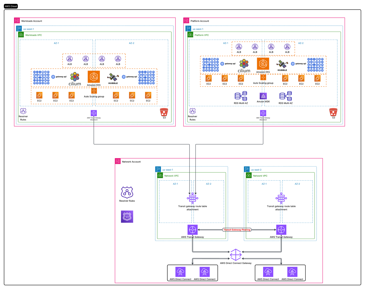
Figure 1: Equinix North Star architecture, a multi-account Amazon EKS architecture with workload isolation, centralized shared services, and hybrid connectivity through AWS Transit Gateway and AWS Direct Connect
Key architecture capabilities
The North Star architecture implements a multi-account, shared services model on Amazon EKS that cleanly separates concerns between application teams and the cloud operations team. The diagram illustrates the user acceptance testing (UAT) environment, with identical patterns replicated across non-production (system integration testing and development) and production, built around three core AWS accounts:
- Workloads Account (Workloads-VPC): The Workloads account hosts all application team services running on Amazon EKS in a dedicated VPC deployed across two Availability Zones (AZ-1 and AZ-2) in us-west-1 for high availability. Traffic ingress is managed through Application Load Balancer (ALB) with Kubernetes Gateway API (GatewayClass and Gateway resources) providing precise routing to application namespaces. Cilium serves as the Container Network Interface (CNI), enforcing network policies that isolate workloads at the pod level, while Hubble provides real-time network observability across all application traffic flows.
- Platform Account (Platform-VPC): The Platform account is owned and operated by the cloud operations team, housing all shared infrastructure services in a separate VPC. This includes:
- Managed data services: Amazon RDS, Amazon MSK, Amazon OpenSearch Service, Amazon MQ, and Amazon S3 consumed by application workloads across the account boundary.
- CI/CD infrastructure: GitHub Runners deployed as EKS workloads, providing a centralized, self-service pipeline for all application teams.
- Shared services: Capabilities managed centrally and accessible to all application teams.
Traffic ingress to platform services is handled through Network Load Balancer (NLB), with the same
Cilium/Hubble networking and observability stack as the Workloads account.
- Network Account (Network-VPC): A dedicated Network account acts as the connectivity hub, implementing an AWS Transit Gateway architecture that spans two Regions (us-west-1 and us-east-2) with Transit Gateway peering between them. Key networking capabilities include:
- Cross-account connectivity: AWS Transit Gateway attachments connect both the Workloads and Platform VPCs to the central hub, enabling controlled communication between accounts.
- DNS resolution Amazon Route 53 Resolver endpoints (inbound and outbound) in each Availability Zone, with a private hosted zone providing service discovery across the platform.
- Hybrid connectivity: AWS Direct Connect Gateway with dual circuits connecting back to on-premises Equinix border routers through network firewalls for security enforcement.
Results: Measurable impact across the organization
The migration to Amazon EKS delivered clear, measurable outcomes that validated Equinix’s North Star architecture strategy:
|
40% Reduction in operational overhead by eliminating the need to manage Kubernetes infrastructure. AWS now handles upgrades, patching, and high availability automatically. |
4x Increase in deployment frequency, enabling engineering teams to ship features and updates faster, freed from the constraints of infrastructure bottlenecks. |
100% Unified architecture adopted across multiple business organizations, establishing a single, consistent operating model for all containerized workloads. |
Additional operational improvements include:
- Enhanced developer productivity: Standardized CI/CD workflows through centralized GitHub Runners and self-service namespace provisioning reduced friction across the development lifecycle, allowing application teams to deploy independently without cloud operations team intervention.
- Improved observability: Hubble provides unified network flow visibility across both clusters, replacing fragmented, team-specific monitoring.
- Strengthened security posture: Multi-account isolation between application and shared services workloads, combined with Cilium network policies for pod-level segmentation, reduced the scope of potential security incidents and simplified compliance enforcement.
- Accelerated onboarding: New application teams onboard to the North Star architecture in days rather than weeks, deploying into pre-configured namespaces with access to shared data services, CI/CD pipelines, and observability. They do this without provisioning or managing cluster infrastructure.
“Amazon EKS gave us the foundation we needed to establish our North Star architecture – a scalable, standardized infrastructure that lets our engineers focus on what matters most: delivering innovation for our customers.”
Conclusion
Equinix’s migration to Amazon EKS from a self-managed environment demonstrates how leading digital infrastructure companies are using managed services from AWS to eliminate undifferentiated operational work and redeploy engineering talent toward higher-value innovation.
The North Star architecture now serves as Equinix’s blueprint for scaling containerized workloads across additional business organizations and geographies. It is an architecture that grows with the company while maintaining the governance, security, and operational consistency that enterprise-scale infrastructure demands.
If you are managing complex, distributed infrastructure, the broader takeaway is this: when you consolidate operational ownership onto a well-architected infrastructure and remove the burden of cluster management from your application teams, you can achieve a markedly different pace of innovation.
To get started with your own Amazon EKS deployment, visit the Amazon EKS product page or follow the Getting started with Amazon EKS guide. You can also explore the EKS Best Practices Guide for recommendations on multi-tenancy, networking, and security.
About the authors
Planning for disaster recovery using AWS Local Zones and AWS Outposts racks
Post Syndicated from Brianna Rosentrater original https://aws.amazon.com/blogs/compute/planning-for-disaster-recovery-using-aws-local-zones-and-aws-outposts-racks/
AWS customers with data residency, low latency, or local data processing requirements can use AWS Hybrid Cloud services to run their workloads either on-premises or within their regulatory boundary. Many of these workloads might be critical to their business, with minimal thresholds for downtime.
This post provides practical design guidance for building highly available architectures that span either two AWS Outposts racks or an Outpost rack and an AWS Local Zone, which are physically designed without single points of failure. By distributing workloads across two geographically and logically independent edge locations, you can achieve high availability while still benefiting from the low-latency, data-residency, and on-premises integration advantages that edge infrastructure provides. To maintain high availability, we recommend that you put a disaster recovery (DR) plan in place and conduct regular DR drills with your applications.
The architectures presented here cover a range of approaches to failure detection and site switching. Each approach offers a different balance between Recovery Time Objective (RTO) and Recovery Point Objective (RPO), operational complexity, and cost. By understanding these trade-offs, you can select the architecture that best aligns to your RPO/RTO targets, data protection and residency requirements, and budget. This helps you achieve the resilience your business requires without over-engineering or over-spending.
Overview
Outposts and Local Zones function as extensions of a single Availability Zone (AZ) within the AWS Region they’re anchored to. For high availability when planning for failover between the two platforms, anchor each to a different parent Region or, at minimum, a different AZ within the same Region. This geographic separation supports the low RPO and RTO targets required for mission-critical workloads. The architectures in this post follow these principles:
- Shared responsibility: AWS manages the Outposts and Local Zone infrastructure. You provide resilient power, cooling, and network connectivity for Outpost sites, and implement application-level failover logic.
- Independent failure domains: Treat each site as an independent failure domain. Anchoring each to a different parent AZ (or Region) ensures a failure in one AZ doesn’t affect both sites.
- Resilient network connectivity: Local Zones connect to their parent Region through the AWS Global Network, designed for maximum resilience. Outpost racks include redundant Outpost Networking Devices (ONDs) with eBGP peering for multipath load balancing and failover.
- Capacity planning for N+1: Provision additional capacity beyond your expected workload so surviving instances can absorb the load during host failures without degradation.
Building blocks of a disaster recovery strategy
A key design consideration is how quickly the architecture can detect a site failure and redirect traffic, and what layers of your workload need protection. Your RPO and RTO needs govern this requirement. This post covers three approaches to disaster recovery at different layers of your application, each offering a different balance between time-to-recovery and operational complexity:
- Active/passive DNS-based failover with Amazon Route 53 health checks.
- Active/active architecture using physical or virtual load balancers deployed at each site.
- Hybrid database recovery using native database engine replication with Amazon Relational Database Service (Amazon RDS).
Depending on your workload, you can implement a combination of these strategies to support the various layers of compute and storage of your application.
Active/passive DNS-based failover with Amazon Route 53 health checks
If your workload consists of on-premises web servers accessible from the internet or internal network, you can use a DNS-based failover approach to reroute traffic to a healthy web server in the event of a hardware failure or site outage. Although this method supports any DNS service, the following architecture example uses Amazon Route 53.
DNS-based failover supports two primary approaches. The first is health check routing, where DNS resolves requests to the IP address of a known good service endpoint. The second is multi-value routing, where the DNS service returns multiple IP addresses. Clients attempt connection to the first address and automatically fail over to subsequent addresses if the connection times out. Route 53 health checks continuously monitor endpoint availability. When a site becomes unreachable, Route 53 automatically updates DNS responses to route traffic to the surviving site. This approach is globally available and works across both Outposts and Local Zones.
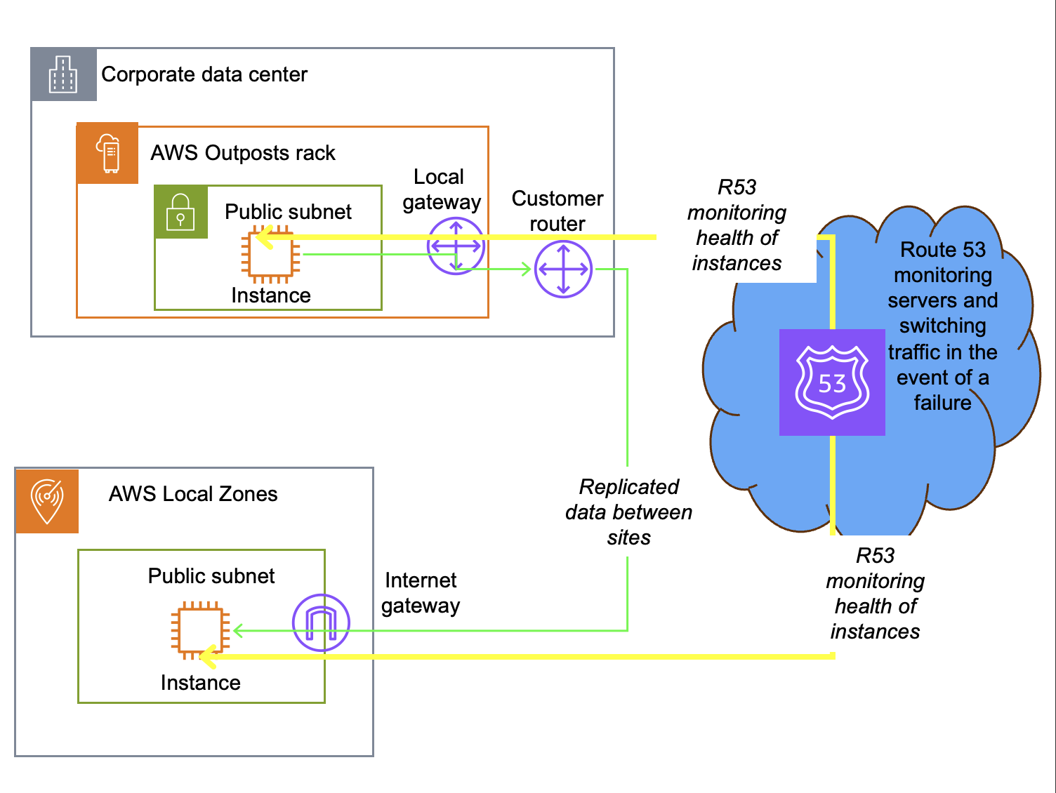
Figure 1: Active/passive DNS-based failover architecture
When a specific application server fails and Route 53 determines it is unreachable, it is dynamically removed from future DNS responses. DNS systems typically have a Time to Live (TTL) of 300 seconds or longer, during which the DNS resolution is cached locally in the client. During this window, the client uses the cached IP address. New requests are automatically directed to active servers. The total recovery time is governed by the combination of the DNS TTL and health check timeout settings, typically resulting in a recovery time of 5 minutes or the TTL setting.
This design pattern works between Outposts, between an Outpost and a third-party provider, between an Outpost and a Local Zone, or between Local Zones. Route 53 can also distribute traffic across these sites, supporting blue/green deployments where you gradually shift traffic from one environment to another.
For AWS Outposts, you can configure Route 53 to monitor an endpoint in the Region. If the Outpost service link disconnects for more than 5 minutes, DNS failover routes traffic to the secondary site. The Outpost and Local Zone can be anchored to the same or different Regions for added resiliency.
As with all architectures using the public internet for replication traffic, configure Transport Layer Security (TLS) encryption in transit, security groups, and network access control lists (NACLs) to secure your data and control access to your subnet resources.
Active/active architecture using physical or virtual load balancers
For Outposts-to-Outposts high availability when your workload must remain on-premises, an alternative to DNS-based failover is an active/active architecture using physical or virtual load balancers deployed at each site. Outposts racks support Application Load Balancer (ALB) as well as third-party L4 and L7 virtual or physical load balancers. Like the DNS-based architecture pattern, you can use this strategy to support workloads that consist of on-premises web servers with low latency, data residency, or continued operations requirements.
In this model, both Outposts can simultaneously serve application traffic, with load balancers continuously monitoring the health of instances. When a failure is detected, the load balancer automatically shifts all traffic to the available Outpost without manual intervention or DNS propagation delays. Typically, the load balancers present a single IP address to service consumers and switch traffic when an endpoint is unavailable. Some load balancers can monitor load and switch traffic based on utilization to maintain response time. This design pattern is specific to Outposts, which support third-party devices connected on premises. It does not work with Local Zones, which are hosted in AWS datacenters.
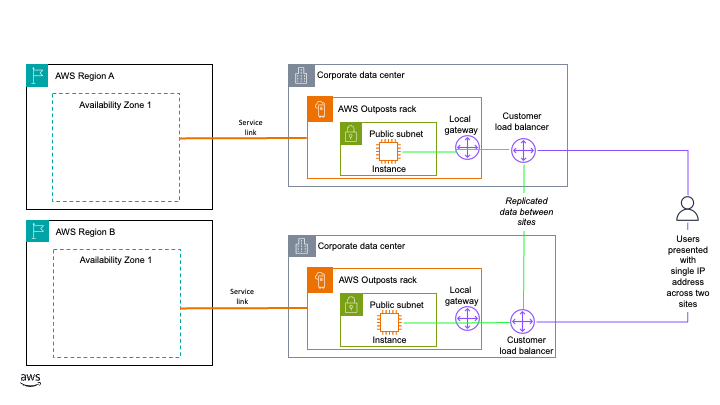
Figure 2: Active/active architecture using physical or virtual load balancers
When you deploy this architecture, make sure the load balancer tier itself does not become a single point of failure. Deploy redundant load balancer instances at each Outpost, with failover between them, so the traffic management layer stays available even if one load balancer instance fails. We also recommend that you configure session persistence and connection draining on your load balancers to minimize disruption to in-flight requests during failover. With this approach, load balancer instances route traffic to your Outpost instances over the local gateway of each Outpost. Traffic continues to be balanced between instances on each Outpost even if one of the Outposts loses its service link connection. You can anchor the Outposts to the same or different Availability Zones or Regions for added resiliency. This approach does require 2N infrastructure and an external load balancer, making it the most resource-intensive to implement.
Some load balancers also support multiple endpoint monitoring. The load balancer monitors both the regional instance and the local application. If the service link fails, based on the administrator’s policy, it can drain connections and route traffic to the other Outpost. This keeps service status and logging fully available on the connected Local Zone or Outpost.
Hybrid database recovery using native database engine replication
If you have two or more logical Outpost racks, you can deploy Amazon RDS on AWS Outposts with Multi-AZ high availability. However, depending on your workload criticality, number of sites, and site locations, a more cost-effective disaster recovery option using one Outpost, one Local Zone, or both might be appropriate. For applications that require a database, you can use your chosen database engine’s native replication features or third-party tooling to create hybrid database architectures across an Outpost and a Local Zone, an Outpost and the Region, or a Local Zone and the Region. If using the Region for failover, this can be the same Region your Outpost or Local Zone is anchored to, or a different Region of your choosing. Limitations based on your chosen database engine and licensing terms apply. In this post, all architecture patterns use a PostgreSQL database. The following three hybrid database strategies expand on the hybrid database with Amazon RDS and AWS Outposts architecture to show how this design pattern supports disaster recovery across Outposts, Local Zones, and AWS Regions.
These architectures use a bring-your-own-license (BYOL) model. The replica instance used for high availability and disaster recovery (HA/DR) is customer-managed, running on Amazon Elastic Compute Cloud (Amazon EC2) and Amazon Elastic Block Store (Amazon EBS). The primary database instance can also be customer-managed, or it can be an RDS-managed database instance so you can use a managed service as your primary operating model. Promoting a replica to primary after a failure is a manual process, but you can automate it with infrastructure as code. Promotion requires updating your DNS entry for the database instance.
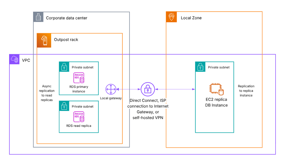
Figure 3: Database failover from an Outpost rack to a Local Zone
In the preceding diagram (Figure 3), the Outpost and the Local Zone can be in the same or different Regions for added resiliency.
In the following diagram (Figure 4), replication traffic can use either the service link or the local gateway of the Outpost as its network path. Replication continues through the local gateway even if the service link fails. If using the service link, the EC2 replica database instance must be in the Outpost anchor Region. If using the local gateway, the EC2 replica database instance can be in the same Region as or a different Region from the Outpost anchor Region for added resiliency. You need to configure a Virtual Private Gateway, Transit Gateway, or Internet Gateway in the Region to receive the replication traffic from the Outpost.
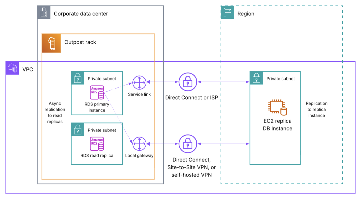
Figure 4: Database failover from an Outpost rack to an AWS Region
In the following diagram (Figure 5), both the primary database instance and the replica are self-hosted on EC2 and EBS. Check your specific Local Zone location for currently supported services to see if the primary database instance can use RDS. The Region used for the EC2 replica DB instance can be the same Region the Local Zone is a part of, or a different Region for added resiliency. If using a different Region, additional networking such as an Internet Gateway is required.
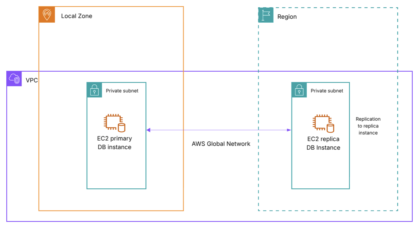
Figure 5: Database failover from a Local Zone to an AWS Region
In all three architectures, you need to update your DNS records and routing to complete failover to the secondary location. If your workload requires data residency, consider whether you can use an AWS Region as a failover destination.
Disaster recovery overview
The strategies discussed in this post support different RTO/RPO objectives. Recovery time depends on the amount of effort to redeploy or reroute to an alternate environment, and whether this process is manual or automated. Recovery point depends on whether the workload has persistent data that needs to be replicated, whether that replication happens synchronously or asynchronously, and whether you use a backup and restore approach. The following table is a high-level overview of the RTO/RPO you can expect for each approach based on these factors:
| Architecture | RTO | RPO |
| Active/passive DNS-based failover | Total failover time = DNS TTL + (health check interval x failure threshold) | Equal to replication schedule, or backup interval |
| Active/active with load balancers | Seconds, traffic is already being routed to both environments | Seconds, data is already being synchronously replicated between sites |
| Hybrid database (same anchor Region) | Minutes, time needed to reroute to replica instance | Equal to replication schedule, faster replication window expected for data traveling less distance |
| Hybrid database (different anchor Region) | <1 hour, time needed to reroute to replica instance | Equal to replication schedule, longer replication window expected for data traveling a greater distance |
Table 1: RTO/RPO disaster recovery overview for each architecture
For the active/passive DNS-based failover architecture, DNS TTL, Route 53 health check interval, and failure threshold are all settings you configure to your preferences. The default Route 53 health check interval is 30 seconds, but can be set as low as 10 seconds. The default Route 53 failure threshold is 3 failed checks, but can be set to any number between 1 to 10. Generally, active/active architectures provide the lowest RTO/RPO for your workloads, whereas active/passive architectures incur some downtime during a disaster when rerouting user traffic to your passive standby environment. Review your workload RTO/RPO objectives to determine which approach is right for you. You might require different strategies for different tiers of workload based on your threshold for downtime at each tier.
Considerations
When choosing a disaster recovery strategy, consider:
- Latency impact based on the location of your failover site and where your application users are.
- Resilient network connectivity between your primary and secondary failover locations, or between your on-premises site and the AWS Region. Architecture-specific guidance is included in each section.
- If your workload requires data residency, evaluate if a particular disaster recovery approach can be used.
- Promoting a replica (either RDS-managed or customer-managed) is a manual process that you can automate with infrastructure as code, and it requires updating your DNS entry for the database instance.
- Database replicas might support synchronous or asynchronous replication depending on the database engine. Consider your RPO objectives when evaluating the hybrid database architectures.
- Limitations based on your chosen database engine and licensing terms apply. Consult your licensing terms and conduct failover drills to test these architecture patterns with your workloads before implementing into production.
Conclusion
This post showed different architecture patterns for disaster recovery using both Outposts and Local Zones. See Building highly resilient applications with on-premises interdependencies using AWS Local Zones for additional guidance. Reach out to your AWS account team to learn more about the hybrid edge architectures discussed in this post. To discuss Outposts with an expert on any of these topics, submit the AWS Outposts contact form. To begin using Local Zones, enable a Local Zone from your account and start experimenting.
Conversations With Maggie Haberman and Jonathan Swan
Post Syndicated from The Atlantic original https://www.youtube.com/watch?v=wXJA4SmI8wg
Inside the lab where the Arm AGI CPU is brought to life
Post Syndicated from Patrick Kennedy original https://www.servethehome.com/inside-the-lab-where-the-arm-agi-cpu-is-brought-to-life/
We travel to the Arm ATE lab to see what goes into bringing up a new Arm server processor, the Arm AGI CPU. It is lab tour time!
The post Inside the lab where the Arm AGI CPU is brought to life appeared first on ServeTheHome.
Deploying regulated workloads on AWS Local Zones and AWS Outposts
Post Syndicated from Brianna Rosentrater original https://aws.amazon.com/blogs/compute/deploying-regulated-workloads-on-aws-local-zones-and-aws-outposts/
Customers in many industries and geographic locations have specific data sovereignty and residency objectives. AWS Local Zones and AWS Outposts are fully managed infrastructure solutions for customers that need to keep data within specific geographic boundaries and also want the scalability and innovation of cloud services. The challenge lies not only in where data resides, but in how to architect, secure, and audit these deployments effectively. Whether you’re architecting a new solution or migrating existing regulated workloads to AWS hybrid edge infrastructure, this post provides an overview of key technologies to help you build auditable and secure architectures that support your organization’s data residency objectives.
Solution framework
Building a solution for data residency deployments on AWS hybrid infrastructure requires a thoughtful, layered approach. Rather than a prescriptive solution, this post presents a flexible framework that you can adapt to your specific operational requirements.
The AWS Shared Responsibility Model clearly delineates where the responsibilities of AWS end and yours begin. This model provides a critical separation: AWS controls the management infrastructure, while your data remains inaccessible to AWS operators, as enforced by the hardware-based isolation of the Nitro System. There is no operator access to the instances, applications, or data. This architectural separation provides the foundation for implementing stringent data residency controls.
To build upon this foundation, you can implement security best practices by following the guidance in the AWS Well-Architected security pillar, which helps you strengthen application-level protections and data security controls. For deeper guidance, see the Data Residency with Hybrid Cloud Services Lens, which covers considerations for operations, security, cost, performance, and reliability for regulated workloads.
When implementing data residency controls, you might need auditable evidence of traffic patterns for your internal governance processes. By using third-party monitoring tools combined with port mirroring capabilities, you can generate reports that show all traffic between your applications and databases remains within your Outpost environment. This visibility provides auditable evidence that traffic remains within your designated boundaries. You can also use AWS Artifact to access audit reports for your hybrid infrastructure.
Governance tools form the final layer of this regulatory framework, establishing guardrails around your deployment. These tools continuously monitor and enforce configuration policies, verifying that your environment stays aligned with your security and governance policies, operates within required parameters, and alerts you proactively when issues arise. This shift from reactive to proactive management helps you maintain consistent governance of your environment at scale.
Together, these layered technologies create a framework for deploying regulated workloads designed to support your data residency objectives while benefiting from the innovation and scalability of AWS services.
Shared responsibility model
When extending workloads to Local Zones and Outposts, the shared responsibility model adapts to these hybrid cloud environments while maintaining the same core principles. AWS continues to manage the underlying infrastructure and services, while you retain control over your data, applications, and configurations. This supports consistent security postures whether workloads run in AWS Regions, Local Zones, or on Outposts infrastructure. You deploy Outposts in a data center or colocation facility of your choice. Under the shared responsibility model, you are responsible for meeting site requirements for power, cooling, on-premises networking, and the Outpost service link connection to the Region. All traffic between the Outpost and the parent Region traverses an encrypted set of VPN connections over the service link, protecting communications in transit without requiring additional configuration. AWS continues to be responsible for maintaining the Outposts hardware as a managed service.
This partnership approach to security means you can build auditable solutions with data residency controls without compromising on the innovation and scalability that AWS provides.
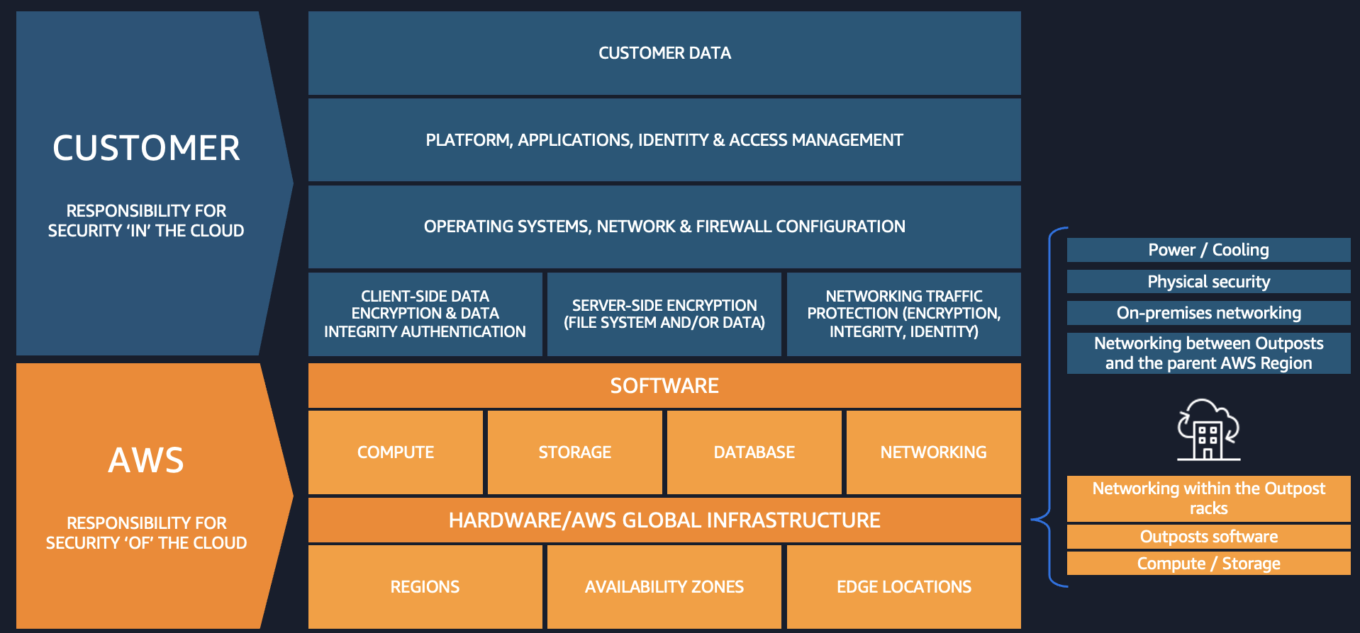
Figure 1: The AWS Shared Responsibility Model in a hybrid edge deployment
AWS Nitro System
The AWS Nitro System is the virtualization platform that powers Amazon Elastic Compute Cloud (Amazon EC2) instances. It uses dedicated hardware and software to offload virtualization functions from the server CPU and delivers near-bare-metal performance. Both Outposts and Local Zones also use the Nitro System. By design, the Nitro System has no operator access. There is no way for AWS or any entity to log into the EC2 Nitro hosts, access compute resources, or reach encrypted customer data remotely. The following diagram shows the purpose-built hardware components of the Nitro System.
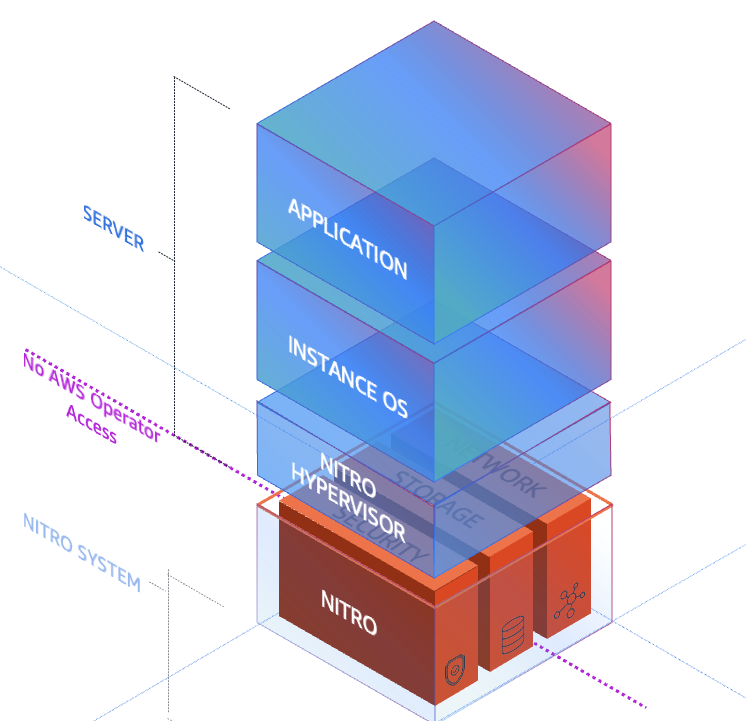
Figure 2: The AWS Nitro System hardware and software stack
The Nitro System combines purpose-built hardware consisting of the following key security components:
- The Nitro Card – provides I/O interfaces used for Amazon Virtual Private Cloud (Amazon VPC) network virtualization, Amazon Elastic Block Store (Amazon EBS), and instance storage, freeing up host CPU resources. Nitro Cards are logically isolated from the system main board that runs customer workloads and can be live-updated, reducing the need for maintenance windows and workload disruption.
- The Nitro Security Chip – provides the link between the Nitro Controller (used for orchestration) and the system main board. It intercepts and controls all firmware updates, preventing the main CPUs from being used to modify system firmware. This is particularly important when running bare metal EC2 instances. This chip is also used for boot control to validate system firmware integrity.
- The Nitro Hypervisor – designed to receive EC2 instance management commands sent by the Nitro Controller, provide compute virtualization and logical instance isolation, and assign SR-IOV virtual functions as needed. It includes no general-purpose operating system features, only the features absolutely necessary for its function, and works with other purpose-built Nitro components to maintain its small size and bare-metal-like performance. This simple design reduces the risk for remote networking attacks and driver-based privilege escalations.
- The Nitro Security Key (Outposts only) – a removable device that stores the external key required to decrypt all data at rest on your Outpost. At the end of your Outposts commitment, after migrating your data off the Outpost, you can destroy this key to cryptographically shred any remaining data on the Outpost.
These components work together to provide a layered security approach that doesn’t compromise performance. By designing each component to have a specific function decoupled from the main system board, the Nitro System provides non-disruptive firmware updates and reduces classes of security issues often found in other hypervisor systems.
AWS Organizations Service Control Policies
AWS Organizations Service Control Policies (SCPs) are a governance tool that helps you enforce data residency requirements by controlling where resources can be created and where data can be stored or processed. SCPs function as permission guardrails that define the maximum available permissions for IAM users and roles across your organization’s accounts. By implementing deny guardrails through SCPs, you can prevent resource provisioning in unwanted locations by restricting access to AWS APIs at the infrastructure level.
When deploying regulated workloads on Local Zones and Outposts, SCPs work in conjunction with AWS Control Tower landing zones to create custom guardrails that control data movement, processing, and storage. These policies can be designed with either preventative rules (blocking actions before they occur) or detective rules (identifying compliance violations after the fact). SCPs can restrict data transfer, saving, or snapshot creation outside a specified AWS location, and they can isolate workloads to a specific location. You can apply SCPs across accounts and organizational units (OUs) within your organization. For more information, see Best practices for managing data residency in AWS Local Zones using landing zone controls and Architecting for data residency with AWS Outposts rack and landing zone guardrails.
Here’s an example SCP that restricts EC2 instance launches and network interface creation to only specified AWS Local Zone subnets:
Compliance monitoring
After you implement the security and governance best practices described in the preceding sections, you can demonstrate that traffic remains within your designated boundaries by using Amazon VPC Traffic Mirroring (also called port mirroring outside of AWS). This mirrors traffic between your application servers and databases. You can use a mirror target report to show that the traffic does not transit the AWS Region. For step-by-step instructions, see Get started using Traffic Mirroring to monitor network traffic. The key configuration steps include the following:
- Configure security groups – Allow inbound UDP port 4789 only from the security group of the source instances being mirrored, or from specific private CIDR ranges within the VPC. Do not open this port to
0.0.0.0/0. - Create a traffic mirror target – Use the elastic network interface (ENI) of your monitoring instance.
- Create a traffic mirror filter – Define which traffic to capture, either all traffic or specific traffic.
- Create mirror sessions – Create one for each source instance you want to monitor. Lower session numbers are evaluated first when multiple sessions exist.
- Capture traffic – Use
tcpdumpon the target instance to analyze mirrored packets.
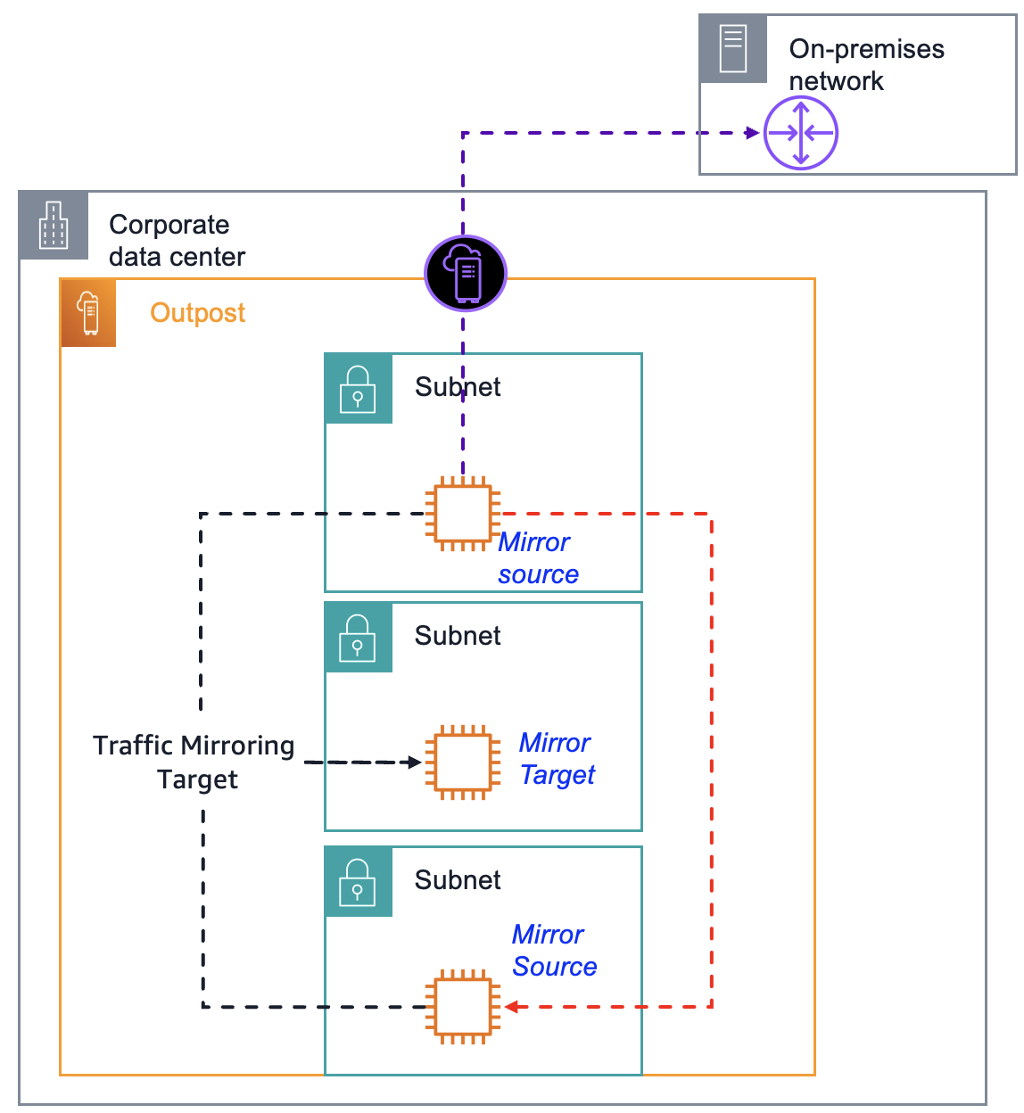
Figure 3: Amazon VPC Traffic Mirroring architecture on an Outpost
All instances must be in the same VPC, or connected through VPC peering or an AWS Transit Gateway. Traffic Mirroring encapsulates the mirrored traffic using VXLAN on UDP port 4789. Traffic Mirroring might impact network performance on source instances, so test in a development environment before deploying to production. The following image shows a sample traffic mirroring report that uses NetFlow Analyzer. For this post, all network traffic shown is simulated.
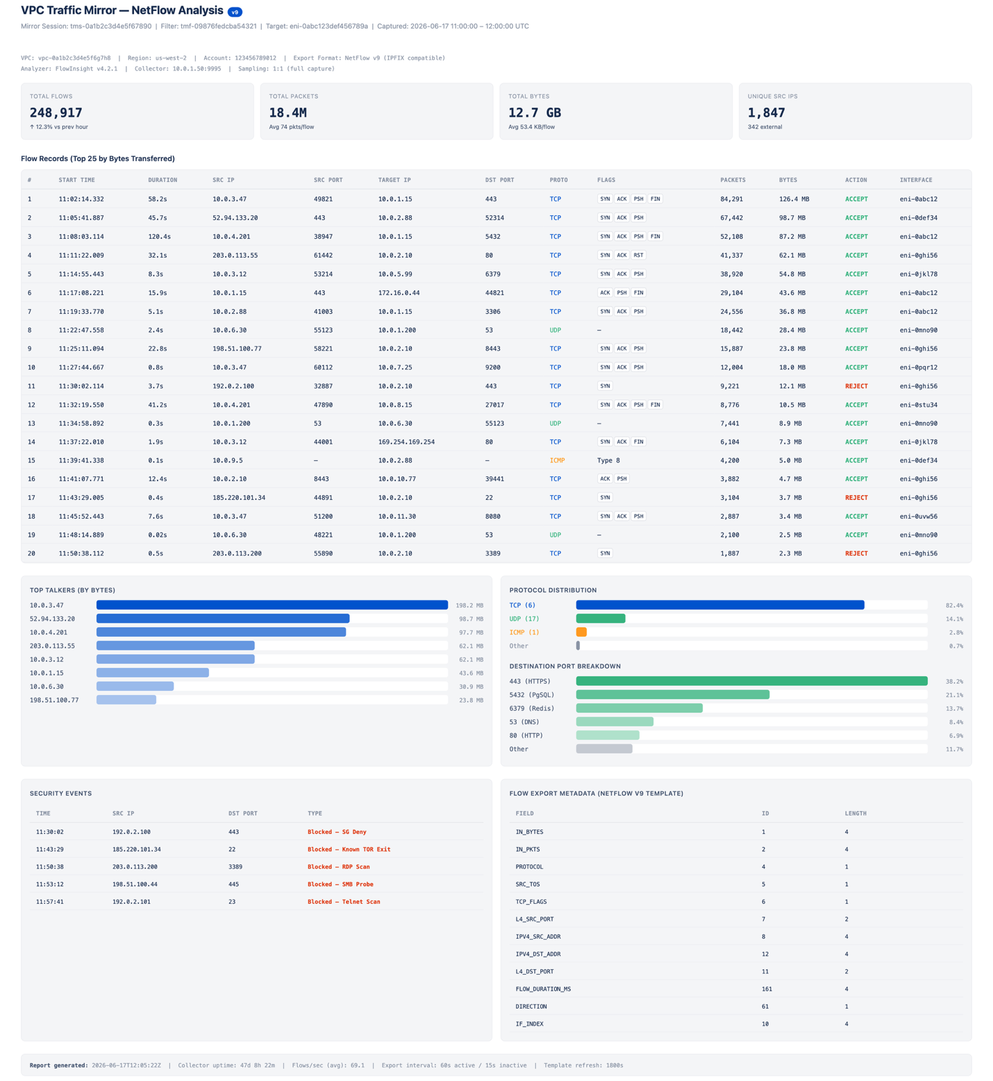
Figure 4: Sample traffic mirroring report in NetFlow Analyzer
Clean up
If you tested the VPC Traffic Mirroring architecture described in the preceding section, terminate any unnecessary resources to avoid ongoing costs. Remove the resources in the following order to avoid dependency errors:
- Delete the traffic mirror sessions – In the Amazon VPC console, navigate to Traffic Mirroring, Mirror Sessions. Select each mirror session you created and choose Actions, Delete. Repeat for all sessions associated with your source instances.
- Delete the traffic mirror filter – Navigate to Traffic Mirroring, Mirror Filters. Select the filter you created and choose Actions, Delete. You must delete all associated mirror sessions before you can delete the filter.
- Delete the traffic mirror target – Navigate to Traffic Mirroring, Mirror Targets. Select the target pointing to the ENI of your monitoring instance and choose Actions, Delete.
- Revoke security group rules – Navigate to Security Groups and select the security group attached to your monitoring instance. Remove the inbound rule that allows UDP port 4789 from the security group or CIDR range of the source instances.
- Terminate the monitoring instance (optional) – If you launched a dedicated EC2 instance solely for traffic capture and analysis, navigate to the EC2 console and terminate the instance. This also releases the associated ENI used as the mirror target.
- Delete any stored packet captures (optional) – If you saved
tcpdumpoutput to Amazon Simple Storage Service (Amazon S3) or local storage on the instance, delete those files if they are no longer needed for audit reporting.
You can verify that all Traffic Mirroring resources have been removed by running the following AWS Command Line Interface (AWS CLI) commands:
Each command should return an empty list, confirming that no mirroring resources remain active in your account.
Conclusion
In this post, we covered how the AWS Nitro System, AWS Organizations SCPs with an AWS Control Tower landing zone, and VPC Traffic Mirroring provide capabilities for governing workloads with data residency requirements. Apply the SCP example in this post to test restricting instance launches and network interface creation to specific subnets. To learn more about Outposts for hybrid deployments, review the Getting started with AWS Outposts guide and submit the AWS Outposts contact form. To get started with Local Zones, review the Getting started with AWS Local Zones guide, opt in to a Local Zone, and begin trying some of the architecture patterns described in this post.
A Conversation With Secretary Pete Buttigieg
Post Syndicated from The Atlantic original https://www.youtube.com/watch?v=M9UZ7ZGD2vE
Building my own solar test bench #solar #diy #offgrid
Post Syndicated from Crosstalk Solutions original https://www.youtube.com/shorts/tpElhU93Spk